essays on archaic institutions and modern technologyetheses.lse.ac.uk/515/1/natraj_essays on archaic...

Essays on Archaic Institutions and Modern

Technology

Ashwini Natraj

November 30, 2012

A thesis submitted to the Department of Economics of the London

School of Economics for the degree of Doctor of Philosophy, London

Declaration

I certify that the thesis I have presented for examination for the PhD degree of the

London School of Economics and Political Science is solely my own work other than

where I have clearly indicated that it is the work of others (in which case the extent

of any work carried out jointly by me and any other person is clearly identified in

it).

The copyright of this thesis rests with the author. Quotation from it is permitted,

provided that full acknowledgement is made. This thesis may not be reproduced

without the prior written consent of the author.

I warrant that this authorization does not, to the best of my belief, infringe the

rights of any third party.

I declare that my thesis consists of 35707 words.

London, November 30, 2012

Ashwini Natraj

1

Contents

Acknowledgements 7

Abstract 9

Introduction 11

I Overview . . . . . . . . . . . . . . . . . . . . . . . . . . . . . . . . . . . 11

II Chapter Summaries . . . . . . . . . . . . . . . . . . . . . . . . . . . . . 12

II.1 Chapter 1 . . . . . . . . . . . . . . . . . . . . . . . . . . . . . . 12

II.2 Chapter 2 . . . . . . . . . . . . . . . . . . . . . . . . . . . . . . 12

II.3 Chapter 3 . . . . . . . . . . . . . . . . . . . . . . . . . . . . . . 13

III Contributions to the Literature . . . . . . . . . . . . . . . . . . . . . . 14

III.1 Chapter 1 . . . . . . . . . . . . . . . . . . . . . . . . . . . . . . 14

III.2 Chapter 2 . . . . . . . . . . . . . . . . . . . . . . . . . . . . . . 15

III.3 Chapter 3 . . . . . . . . . . . . . . . . . . . . . . . . . . . . . . 15

List of tables 16

List of figures 18

1 Some Unintended Consequences of Political Quotas 20

1.1 Introduction . . . . . . . . . . . . . . . . . . . . . . . . . . . . . . . . . 20

1.2 Theoretical Predictions about Turnout, Electoral Competition and Party

Bias . . . . . . . . . . . . . . . . . . . . . . . . . . . . . . . . . . . . . . 25

1.2.1 Ratio of Candidates to Electors . . . . . . . . . . . . . . . . . . 25

2

1.2.2 Margin of Victory . . . . . . . . . . . . . . . . . . . . . . . . . . 26

1.2.3 Turnout . . . . . . . . . . . . . . . . . . . . . . . . . . . . . . . 26

1.2.3.1 Competition . . . . . . . . . . . . . . . . . . . . . . . 26

1.2.3.2 Expressive Voting . . . . . . . . . . . . . . . . . . . . 27

1.2.3.3 Identity as Information . . . . . . . . . . . . . . . . . 27

1.2.4 Party Bias . . . . . . . . . . . . . . . . . . . . . . . . . . . . . . 28

1.2.4.1 Candidates . . . . . . . . . . . . . . . . . . . . . . . . 28

1.2.4.2 Voters . . . . . . . . . . . . . . . . . . . . . . . . . . . 29

1.3 Reservation in India . . . . . . . . . . . . . . . . . . . . . . . . . . . . . 29

1.4 Identification Strategy . . . . . . . . . . . . . . . . . . . . . . . . . . . 30

1.4.1 Construction of Treatment and Control Groups (SC constituen-

cies) . . . . . . . . . . . . . . . . . . . . . . . . . . . . . . . . . . 31

1.4.2 Construction of Treatment and Control Groups (ST constituen-

cies) . . . . . . . . . . . . . . . . . . . . . . . . . . . . . . . . . . 31

1.5 Empirical Specification . . . . . . . . . . . . . . . . . . . . . . . . . . . 32

1.6 Data . . . . . . . . . . . . . . . . . . . . . . . . . . . . . . . . . . . . . . 32

1.6.1 Summary Statistics: Village Averages . . . . . . . . . . . . . . 33

1.6.2 Summary Statistics: Constituency Averages . . . . . . . . . . . 33

1.7 Results: Aggregate . . . . . . . . . . . . . . . . . . . . . . . . . . . . . 35

1.7.1 Basic Results . . . . . . . . . . . . . . . . . . . . . . . . . . . . . 35

1.7.2 Robustness Checks . . . . . . . . . . . . . . . . . . . . . . . . . 36

1.7.2.1 Placebo Checks . . . . . . . . . . . . . . . . . . . . . . 37

1.7.2.2 Widening the sample . . . . . . . . . . . . . . . . . . 37

1.7.2.3 Districts with both Treated and Untreated Constituen-

cies . . . . . . . . . . . . . . . . . . . . . . . . . . . . . 37

1.8 Individual-level Voting . . . . . . . . . . . . . . . . . . . . . . . . . . . 38

1.8.1 Summary Statistics for Lokniti Constituencies: Respondent Char-

acteristics in 2008 . . . . . . . . . . . . . . . . . . . . . . . . . . 39

1.8.2 Results: Individual Voting Data . . . . . . . . . . . . . . . . . . 40

3

1.8.3 Magnitude of Effects . . . . . . . . . . . . . . . . . . . . . . . . 41

1.8.4 Interpretation . . . . . . . . . . . . . . . . . . . . . . . . . . . . 42

1.8.4.1 Competition . . . . . . . . . . . . . . . . . . . . . . . 42

1.8.4.2 Expressive Voting . . . . . . . . . . . . . . . . . . . . 42

1.8.4.3 Information . . . . . . . . . . . . . . . . . . . . . . . . 42

1.9 Conclusion . . . . . . . . . . . . . . . . . . . . . . . . . . . . . . . . . . 43

2 Why do Workers Remain in Low-Paying Hereditary Occupations? 44

2.1 Introduction . . . . . . . . . . . . . . . . . . . . . . . . . . . . . . . . . 44

2.2 Background . . . . . . . . . . . . . . . . . . . . . . . . . . . . . . . . . 47

2.2.1 Caste in India: Ascriptive or not? . . . . . . . . . . . . . . . . . 47

2.2.2 The Joint Family . . . . . . . . . . . . . . . . . . . . . . . . . . 49

2.2.2.1 Filial Responsibility . . . . . . . . . . . . . . . . . . . 49

2.2.2.2 Parental Responsibility . . . . . . . . . . . . . . . . . 50

2.3 Altruism, Asset Poverty or Insurance . . . . . . . . . . . . . . . . . . . 50

2.3.1 Traditional Occupations and Parental Reponsibility . . . . . . 51

2.3.2 Family, Caste and Insurance . . . . . . . . . . . . . . . . . . . . 52

2.4 Model . . . . . . . . . . . . . . . . . . . . . . . . . . . . . . . . . . . . . 54

2.4.1 Model Setup . . . . . . . . . . . . . . . . . . . . . . . . . . . . . 54

2.4.2 The Parent’s Problem . . . . . . . . . . . . . . . . . . . . . . . . 57

2.4.2.1 Results: Maximum Human Capital Transferred by

Parent . . . . . . . . . . . . . . . . . . . . . . . . . . . 58

2.4.3 The Child’s Problem . . . . . . . . . . . . . . . . . . . . . . . . 60

2.4.3.1 Minimum Human Capital Accepted by Child: Inte-

rior Stationary Solution . . . . . . . . . . . . . . . . . 62

2.5 Numerical Simulation . . . . . . . . . . . . . . . . . . . . . . . . . . . 63

2.5.1 Results: Numerical Solution . . . . . . . . . . . . . . . . . . . . 64

2.5.1.1 Parental Human Capital Transfer . . . . . . . . . . . 65

2.5.1.2 Human Capital Accepted by Child . . . . . . . . . . 65

2.5.1.3 Set of Sustainable Human Capital Transfers . . . . . 66

4

2.6 Conclusion . . . . . . . . . . . . . . . . . . . . . . . . . . . . . . . . . . 66

3 Has ICT Polarized Skill Demand? Evidence from Eleven Countries over

25 years 68

3.1 Introduction . . . . . . . . . . . . . . . . . . . . . . . . . . . . . . . . . 68

3.2 Empirical Strategy . . . . . . . . . . . . . . . . . . . . . . . . . . . . . 70

3.3 Empirical Model . . . . . . . . . . . . . . . . . . . . . . . . . . . . . . . 71

3.4 Data . . . . . . . . . . . . . . . . . . . . . . . . . . . . . . . . . . . . . . 74

3.4.1 Data Construction . . . . . . . . . . . . . . . . . . . . . . . . . 74

3.4.2 Descriptive statistics . . . . . . . . . . . . . . . . . . . . . . . . 76

3.4.2.1 The Routineness of Occupations by Skill Level . . . 76

3.4.2.2 Cross Country Trends . . . . . . . . . . . . . . . . . . 77

3.4.2.3 Cross Industry Trends . . . . . . . . . . . . . . . . . . 79

3.5 Econometric Results . . . . . . . . . . . . . . . . . . . . . . . . . . . . 80

3.5.1 Basic Results . . . . . . . . . . . . . . . . . . . . . . . . . . . . . 80

3.5.2 Robustness and Extensions . . . . . . . . . . . . . . . . . . . . 82

3.5.2.1 Initial conditions . . . . . . . . . . . . . . . . . . . . . 82

3.5.2.2 Timing of changes in skills and ICT . . . . . . . . . . 83

3.5.2.3 Heterogeneity in the coefficients across countries . . 83

3.5.2.4 Instrumental variables . . . . . . . . . . . . . . . . . 84

3.5.2.5 Disaggregating the wage bill into wages and hours . 85

3.5.3 Trade, R&D and skill upgrading . . . . . . . . . . . . . . . . . 85

3.5.4 Magnitudes . . . . . . . . . . . . . . . . . . . . . . . . . . . . . 87

3.6 Conclusions . . . . . . . . . . . . . . . . . . . . . . . . . . . . . . . . . 88

Appendices . . . . . . . . . . . . . . . . . . . . . . . . . . . . . . . . . . . . 90

A Figures: Chapter 1 90

B Tables: Chapter 1 93

C Data Appendix: Chapter 1 107

5

D Proofs of Propositions: Chapter 2 109

D.1 Proof of Proposition 1 . . . . . . . . . . . . . . . . . . . . . . . . . . . . 109






E Figures: Chapter 2 116

F Figures: Chapter 3 122

G Tables: Chapter 3 133

H Data Appendix: Chapter 3 146

H.1 Construction of main dataset . . . . . . . . . . . . . . . . . . . . . . . 146

H.2 Construction of task measures by skill . . . . . . . . . . . . . . . . . . 148

Bibliography 150

6

Acknowledgements

Writing a thesis is a complex process, made of frustration and satisfaction in

unpredictable measure. One of the greatest of these satisfactions is the opportunity

to salute the people who have helped me so much along the way.

Firstly, this would have been impossible without the support of my wonderful

parents. I am indebted beyond words to them for their encouragement, warmth,

and several lively discussions about Indian politics, the caste system and family

structure.

I am tremendously obliged to Oriana Bandiera and Gerard Padro-i-Miquel for

their guidance and valuable and incisive insight. They have taught me to think

critically and to question my assumptions. The work that you see would be unrec-

ognizable without them.

Chapter 1 was greatly improved by comments from seminar participants at the

London School of Economics. I am particularly obliged to Guilhem Cassan for leads

regarding data, and to Sanjay Kumar at the Centre for the Study of Developing

Societies, Delhi, for his generosity with individual-level electoral data.

Working on Chapter 3 was tremendously rewarding. I feel extremely privileged

to have worked with Guy Michaels and John Van Reenen at the Centre for Economic

Performance, LSE, and to have learnt so much from them about rigour and critical

thinking in empirical research.

For Chapter 3,we are indebted to David Autor, Tim Brenahan, David Dorn, Liran

Einav, Maarten Goos, Larry Katz, Paul Krugman, Alan Manning, Denis Nekipelov,

Stephen Redding, Anna Salomons, and seminar participants at the AEA, Imperial,

7

LSE, NBER, SOLE-EALE meetings and Stanford for extremely helpful comments.

David Autor kindly provided the data on routine tasks. Finance was provided by

the ESRC through the Centre for Economic Performance.

I am fortunate, too, in my erudite and articulate friends, both at the LSE and

outside it. I am indebted to Barbara Richter and Joachim Groeger for allowing me

to bounce ideas off them and both tolerating and correcting my muddy thinking

and muddier prose. Alex Lembcke and Rosa Sanchis Guarner-Herrero lent me their

time, sympathy and expertise and I am tremendously grateful.

Throughout this process I have had helpful discussions, spirited exchanges and

innumerable cups of tea and coffee with Michael Best, Mirko Draca, Katalin Sze-

meredi, Amy Challen and Iain Long. Research is a collaborative process, and the

nature of collaboration can surprise you. It is a genuine pleasure now to recall how

unexpectedly fruitful a freewheeling conversation can be.

Many thanks to the staff of the British Library, the LSE Library and the libraries

at UCL and SOAS. Their generosity with their time and help dredging up obscure

cartographic, administrative and sociological texts made researching colonial and

modern Indian institutions a pleasure. All my gratitude to Mark Wilbor at the LSE

who made allowances for my poor organization and helped to smooth the path to

submission.

Finally, my long-suffering flatmates have provided me with support, a captive

audience, and a sense of humour and perspective at the most critical of times. I am

very grateful to Arti Agrawal and Sylvie Geroux for their warmth, wit and generos-

ity.

It goes without saying, of course, that all remaining errors are my own.

8

Abstract

I present three essays discussing the impact of archaic institutions and technol-

ogy on inequality in wages and political participation. First I examine a modern

facet of the Indian caste system: political quotas for disadvantaged minorities and

their impact on political participation. I find that aggregate turnout falls by 9% of

the baseline and right-wing parties win 50% more often, but electoral competition is

not significantly affected. Detailed individual-level data for one state suggests that

voter participation falls among women and minorities. This suggests that restricting

candidate identity to minorities may cause some bias in voter participation.

Next, I study caste and human capital: specifically why workers remain in low-

paying hereditary occupations, providing an explanation for both occupational spe-

cialization and hereditary occupations. I use a simple model of insurance provision

in which parents pass on human capital to their children in return for insurance in

the event of sickness, and find that workers with low human capital are likelier to

participate in the arrangement, and that a higher cost of sickness can sustain higher

human capital transfers.

I conclude by studying human capital and technology- the impact of information

and communication technologies (ICT) on wage inequality. We tested the hypoth-

esis that information and communication technologies (ICT) polarize labour mar-

kets, by increasing demand for the highly educated at the expense of the middle

educated, with little effect on low-educated workers. Using data on the US, Japan,

and nine European countries from 1980-2004, we find that industries with faster ICT

growth shifted demand from middle educated workers to highly educated workers,

9

consistent with ICT-based polarization. Trade openness is also associated with po-

larization, but this is not robust to controlling for Research and Development. Tech-

nologies account for up to a quarter of the growth in demand for highly educated

workers.

10

Introduction

I Overview

The following essays consider one of the several paradoxical facets of develop-

ing countries: the tension between ancient institutions and the forces of modernity,

whether they arrive in the form of competition, technology or both. This is particu-

larly striking in India, a country in which rapid technological advancement coexists

sometimes uneasily with the stubborn persistence of archaic institutions. One such

institution is that of the caste system, which has exhibited considerable resilience in

the face of economic growth and urbanisation, and shows every sign of using infor-

mation and communication technology to further entrench itself (as evinced by the

persistence of endogamy in modern India (Banerjee, Duflo, Ghatak, and Lafortune

(2009))).

The first two essays consider two aspects of the caste system. Chapter 1 deals

with an attempt to correct the disenfranchisement of citizens at the bottom of the

caste hierarchy, and Chapter 2 considers the benefits of occupational specialisation

and intergenerational occupational rigidity. The final two chapters consider the ac-

cumulation of human capital first in an environment with imperfect capital markets

and no obsolescence, and second through the lens of Information and Communica-

tion Technologies and their impact on skill demand.

11

II Chapter Summaries

II.1 Chapter 1

A representative democracy should seek to reflect the needs of its entire popu-

lation, but there is a concern that a nation’s elected representatives do not serve the

needs of its most vulnerable citizens. Many countries, concerned that these citizens

are not adequately represented in their governments, have sought to redress the bal-

ance with quotas. Advocates of the policy suggest that the identity of a legislator

affect her policy preferences, so at the least imposing quotas may have redistributive

effects (Pande (2003), Chattopadhyay and Duflo (2004)).

One key assumption made when assessing the impact of quotas on policy prefer-

ences is that quotas change only legislator identity, leaving voter identity unaffected.

Moreover, critics of quotas claim that quotas are by their nature uncompetitive, since

by changing the candidate pool they distort incentives and weaken electoral com-

petition.

In Chapter 1, I use a provision of the Constitution of India to examine the causal

impact of the introduction of quotas for disadvantaged minorities on electoral com-

petition and voter participation, at the level of the constituency, and find that while

quotas have no discernible adverse effect on electoral competition, they depress

turnout. Detailed data for a subsample suggest that quotas depress turnout espe-

cially among women and minorities.

II.2 Chapter 2

While Chapter 1 dealt with a present-day outcome of the caste system, I now turn

attention to one reason for its persistence- intergenerational occupational rigidity as

a means of procuring insurance in the presence of imperfect credit markets.

Occupational rigidity is a much-studied phenomenon. Explanations vary from

the cost of acquiring human capital in the presence of indivisible human capital in-

vestments and capital market imperfections (Bannerjee and Newman (1993)) to the

12

information advantages of family, village, ethnic or occupationally specialized net-

works (Akerlof (1976), Greif (1993), Freitas (2006)). One persuasive explanation is

that social networks provide access to consumption-smoothing (Munshi and Rosen-

zweig (2009)).

I use a two-period Overlapping Generations model in which a parent with an

endowment of occupation-specific human capital transfers costly human capital to

her offspring, in return for full insurance if the parent suffers an accident, with the

penalty for default being a bar from access to to the insurance arrangement. I find

that agents with low human capital are more liable to participate in the insurance

arrangement, and that the maximum sustainable human capital transfer rises with

the cost of sickness.

II.3 Chapter 3

Chapters 2 and 3 deal with two conflicting forces on human capital- in Chapter

2 agents accumulated human capital in order to have a means of insurance against

sickness, in an environment with no obsolescence owing to technology, whereas in

Chapter 3 I consider the impact of Information and Communication Technology on

the demand for workers across varying occupation and education groups.

The demand for highly-skilled workers in the UK, USA and a range of devel-

oped countries has risen significantly in the past three decades, outstripping even

the rise in supply of workers with a college education over the same period. Most

authorities agree that this increase is brought about by technological changes rather

than a shift in trade with low-wage countries.

A persuasive hypothesis is that technical change complements highly-skilled

workers at the benefit of all others, but a more granular view of the wage distribu-

tion suggests that other factors may be in play. An increase in demand for highly-

skilled workers is reflected in higher wages, but interestingly, in the USA, the ratio

of the wages of workers in the 90th percentile to those in the 50th percentile have

risen far faster than those in the 50th percentile to those in the 10th percentile and

13

lower.

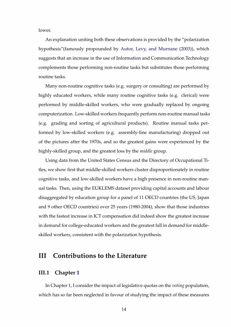
An explanation uniting both these observations is provided by the “polarization

hypothesis”(famously propounded by Autor, Levy, and Murnane (2003)), which

suggests that an increase in the use of Information and Communication Technology

complements those performing non-routine tasks but substitutes those performing

routine tasks.

Many non-routine cognitive tasks (e.g. surgery or consulting) are performed by

highly educated workers, while many routine cognitive tasks (e.g. clerical) were

performed by middle-skilled workers, who were gradually replaced by ongoing

computerization. Low-skilled workers frequently perform non-routine manual tasks

(e.g. grading and sorting of agricultural products). Routine manual tasks per-

formed by low-skilled workers (e.g. assembly-line manufacturing) dropped out

of the pictures after the 1970s, and so the greatest gains were experienced by the

highly-skilled group, and the greatest loss by the middle group.

Using data from the United States Census and the Directory of Occupational Ti-

tles, we show first that middle-skilled workers cluster disproportionately in routine

cognitive tasks, and low-skilled workers have a high presence in non-routine man-

ual tasks. Then, using the EUKLEMS dataset providing capital accounts and labour

disaggregated by education group for a panel of 11 OECD countries (the US, Japan

and 9 other OECD countries) over 25 years (1980-2004), show that those industries

with the fastest increase in ICT compensation did indeed show the greatest increase

in demand for college-educated workers and the greatest fall in demand for middle-

skilled workers, consistent with the polarization hypothesis.

III Contributions to the Literature

III.1 Chapter 1

In Chapter 1, I consider the impact of legislative quotas on the voting population,

which has so far been neglected in favour of studying the impact of these measures

14

on candidates. I provide an understanding of the impact of quotas on electoral com-

petition, how many vote and who votes as a result of quotas. Chapter 1 also con-

tains an analysis of political reservation at the constituency level, which is not only

a meaningful unit of consideration for political variables, but examines permanent

quotas at a more disaggregated level than the state.

III.2 Chapter 2

Chapter 2 provides a simple model of human capital accumulation as a means

of consumption-smoothing, and its theoretical contribution is to unite the views of

castes or guilds as a means of safeguarding human capital or intellectual property

with the more recent literature treating social networks as a means of contract en-

forcement, eradicating information asymmetries or providing insurance.

III.3 Chapter 3

This paper is the first to provide direct international evidence that skills-technology

complementarity benefits highly-skilled workers at the cost of middle-skilled work-

ers, consistent with the polarization hypothesis. Other work has shown a similar

substitution Autor, Levy, and Murnane (2003), Autor and Dorn (2009) but only for

America. Prior to this, Autor, Katz, and Krueger (1998) show that the rise in the use

of computers between 1984 and 1993 was correlated to a fall overall in the demand

for high-school graduates between 1979 and 1993, but we provide evidence for a

panel of 11 countries over a longer time-period.

15

List of Tables

B.1 Constituency Averages: Chhatisgarh, Karnataka, Madhya Pradeshand Rajasthan 2001 . . . . . . . . . . . . . . . . . . . . . . . . . . . . . 93

B.2 Constituency Electoral Characteristics . . . . . . . . . . . . . . . . . . 94B.3 Averages of Dependent Variables . . . . . . . . . . . . . . . . . . . . . 95B.4 Effect of reservation for Scheduled Castes (SCs) in 2008 (Elections

from 2001-2008) . . . . . . . . . . . . . . . . . . . . . . . . . . . . . . . 96B.5 Effect of reservation for Scheduled Castes (SCs) in 2008 (Elections

from 2001-2008) on Incidence of Victory of Party Categories . . . . . 97B.6 Effect of dereservation for Scheduled Castes (SCs) in 2008 (Elections

from 2001-2008) . . . . . . . . . . . . . . . . . . . . . . . . . . . . . . . 98B.7 Effect of reservation for Scheduled Castes (SCs) in 2008 (Elections

from 1993-1999) . . . . . . . . . . . . . . . . . . . . . . . . . . . . . . . 99B.8 Effect of reservation for Scheduled Castes (SCs) in 2008 on success of

political parties (Elections from 1993-1999) . . . . . . . . . . . . . . . 100B.9 Effect of reservation for Scheduled Castes (SCs) in 2008 (Elections

from 2001-2008): 5% cutoff . . . . . . . . . . . . . . . . . . . . . . . . . 101B.10 Effect of reservation for Scheduled Castes (SCs) in 2008 (Elections

from 2001-2008): districts with both treated and untreated constituen-cies . . . . . . . . . . . . . . . . . . . . . . . . . . . . . . . . . . . . . . 102

B.11 Respondent Characteristics: Lokniti Constituencies, Karnataka Post-Poll . . . . . . . . . . . . . . . . . . . . . . . . . . . . . . . . . . . . . . 103

B.12 Constituency Averages at Baseline: Karnataka 2001 . . . . . . . . . . 104B.13 Candidate Characteristics (Lokniti constituencies) . . . . . . . . . . . 105B.14 Individual Voter Participation: Lokniti Karnataka 2008 Post-Poll . . . 106

G.1 Mean Standardized Scores by skill group - 1980 US data . . . . . . . . 133G.2 Top occupations by share of workers of different skill levels, with task

measures . . . . . . . . . . . . . . . . . . . . . . . . . . . . . . . . . . . 134G.3 Summary Statistics by Country . . . . . . . . . . . . . . . . . . . . . . 135G.4 Summary Statistics by Industry: 1980 levels . . . . . . . . . . . . . . . 136G.5 Summary Statistics by Industry: Changes from 1980-2004 . . . . . . . 137G.6 Changes in Wage Bill Shares: 1980-2004 . . . . . . . . . . . . . . . . . 138G.7 Changes in Wage Bill Shares: 1980-2004 - Robustness checks . . . . . 139G.8 Decomposing Changes in Relative Wage Bills into Wages and Hours 140G.9 Trade and Technology . . . . . . . . . . . . . . . . . . . . . . . . . . . 141G.10 List of all EUKLEMS Industries . . . . . . . . . . . . . . . . . . . . . . 142G.11 List of Industries Pooled by Country . . . . . . . . . . . . . . . . . . . 143G.12 Trade, ICT, and Research and Development . . . . . . . . . . . . . . . 144

16

G.13 Contribution of Changes in ICT and R&D to Changes in the High-Skilled Wage Bill Share . . . . . . . . . . . . . . . . . . . . . . . . . . . 145

17

List of Figures

A.1 Allocation of SC seats to a district . . . . . . . . . . . . . . . . . . . . . 90A.2 Identification of District Cutoff . . . . . . . . . . . . . . . . . . . . . . 90A.3 Identification of constituencies close to the threshold . . . . . . . . . 91A.4 Discarding previously-reserved constituencies . . . . . . . . . . . . . 91A.5 Identification of Treatment and Control Groups . . . . . . . . . . . . . 92

E.1 Maximum Human Capital Transferred to Child: h=.18 . . . . . . . . . 116E.2 Maximum Human Capital Transferred to Child: h=.5 . . . . . . . . . 117E.3 Maximum Human Capital Transferred to Child: I=0.01 . . . . . . . . 118E.4 Maximum Human Capital Transferred to Child: I=0.5 . . . . . . . . . 118E.5 Maximum Human Capital Transferred to Child: I=0.99 . . . . . . . . 118E.6 Maximum Human Capital Transfer . . . . . . . . . . . . . . . . . . . . 119E.7 Lower Bound of Maximum Human Capital Transfer . . . . . . . . . . 119E.8 Minimum Human Capital Transfer Accepted by Child . . . . . . . . 120E.9 Difference Between Maximum and Minimum Sustainable Human Cap-

ital Transfers . . . . . . . . . . . . . . . . . . . . . . . . . . . . . . . . . 121

F.1 Cross Country Variation in Growth of High-skilled Wage Bill Sharesand ICT Intensity, 1980- 2004 . . . . . . . . . . . . . . . . . . . . . . . 122

F.2 Cross Country Variation in Growth of Medium-skilled Wage Bill Sharesand ICT Intensity, 1980- 2004 . . . . . . . . . . . . . . . . . . . . . . . 123

F.3 Cross Country Variation in Growth of Low-skilled Wage Bill Sharesand ICT Intensity, 1980- 2004 . . . . . . . . . . . . . . . . . . . . . . . 124

F.4 Average Annual Percentage Point Changes in High, Medium andLow-Skilled Wage Bill Shares over Six- Year Intervals from 1980-2004(Eleven Country Average) . . . . . . . . . . . . . . . . . . . . . . . . . 125

F.5 Average Annual Percentage Point Changes in High, Medium andLow-Skilled Wage Bill Shares over Six- Year Intervals from 1980-2004(U.S. Average) . . . . . . . . . . . . . . . . . . . . . . . . . . . . . . . . 126

F.6 Cross-Industry Variation in Growth of High-Skilled Wage-Bill Shareand ICT Intensity, 1980-2004 (11 Country Means: Whole Economy) . 127

F.7 Cross-Industry Variation in Growth of High-Skilled Wage-Bill Shareand ICT Intensity, 1980-2004 (11 Country Means: Traded Goods Only) 128

F.8 Cross-Industry Variation in Growth of Medium-Skilled Wage-Bill Shareand ICT Intensity, 1980-2004 (11 Country Means: Whole Economy) . 129

F.9 Cross-Industry Variation in Growth of Medium-Skilled Wage-Bill Shareand ICT Intensity, 1980-2004 (11 Country Means: Traded Goods Only) 130

F.10 Cross-Industry Variation in Growth of Low-Skilled Wage-Bill Shareand ICT Intensity, 1980-2004 (11 Country Means: Whole Economy) . 131

18

F.11 Cross-Industry Variation in Growth of Low-Skilled Wage-Bill Shareand ICT Intensity, 1980-2004 (11 Country Means: Traded Goods Only) 132

19

Chapter 1

Some Unintended Consequences of

Political Quotas

1.1 Introduction

Many countries have considered measures to increase the representation of mi-

norities and women, either through quotas or through gerrymandering1. In India,

quotas have been in place for disadvantaged groups since 1951, but the policy’s use

is widespread. In 2010, more than 30 countries in Asia, Africa, South America and

Europe had quotas for women in government.

Proponents of the policy point out that there is reason to believe that nonminor-

ity legislators have different policy preferences from legislators from disadvantaged

groups. So, in addition to considerations of fairness and equity, empirical evidence

suggests that increasing representation for disadvantaged groups may have redis-

tributive effects (Pande (2003), Chattopadhyay and Duflo (2004)).

However, a common assumption made when assessing the impact of legislator

identity on policy is that the imposition of political quotas changes legislator iden-

tity only, while voter identity is unaffected (Pande (2003)). This is a strong assump-

1Section 5 of the Voting Rights Act of America contains provisions that many conservative politi-cians see as racial gerrymandering. See also Shaw v. Reno, 113 S.Ct.2816(1993), in which the SupremeCourt ruled that the creation of a district in North Carolina in which minorities were in the majoritywas unconstitutional.

20

tion, and not innocuous. Critics of quotas, moreover, argue that they are discrimina-

tory, distort incentives and by their nature undermine the democratic process: inter-

vention in order to increase minority representation takes away the right of voters

to choose their representatives freely. Artificially restricting the pool of candidates

weakens electoral competition.

This paper uses a provision of the Constitution of India to examine the causal

impact of the introduction of quotas for disadvantaged minorities on electoral com-

petition and voter participation, at the level of the constituency.

The world’s most comprehensive political affirmative action programme takes

place in India, in which approximately a quarter of all state and national legislators

belong to disadvantaged groups. The representation of members belonging to his-

torically disadvantaged castes (Scheduled Castes or SCs) or tribes (Scheduled Tribes

or STs) is determined according to each decennial census, and the representation of

these groups in the state legislature is held to be as close as possible to their rep-

resentation in the population. Reservation is revisited with the publication of each

decennial census, but not before. When a constituency is reserved for SCs(STs) only

SC(ST) candidates may contest the election, although voters of all identities may

vote.

In 2008, after a long hiatus since 1981, a wave of redistricting (Delimitation) was

carried out, adjusting the representation of SCs and STs in state and national leg-

islatures according to the 2001 census. Four states (Karnataka, Madhya Pradesh,

Rajasthan and Chattisgarh) carried out elections using this adjusted representation.

The documentation released laid out the methodology of reservation transparently,

enabling me to construct for these states a unique dataset with those constituen-

cies which were reserved for the first time in 2008, as well as demographically

and economically comparable constituencies within the same administrative area

which narrowly missed the reservation cutoff and remained unreserved. I use a

Differences-in-Differences approach to examine the impact of political reservation

on turnout, the number of candidates contesting, the margin of victory and the

21

probability of success of right-wing and left-wing parties, as well as those mobil-

ising lower-caste supporters (details in Section 1.2.4).

I find no impact on the number of candidates contesting and no impact on the

margin of victory, so these conventional measures of electoral competition are unaf-

fected by political quotas. However, turnout drops by 6 percentage points relative

to a baseline of 69 percentage points, and right-wing parties make up 26% more

of winners in reserved constituencies after reservation, compared to a baseline of

53%. Results using individual polling data suggest that women vote 15% less, and

minorities vote 9% less, in reserved constituencies after reservation.

There are many possible explanations, but at the very least this evidence suggests

that there are unintended consequences to political quotas- although most standard

measures of electoral competition are unaffected, voter participation falls, and seem-

ingly among the most vulnerable members of the population.

This is a concern, because for a complete picture of the impact of minority repre-

sentation on policy it seems reasonable to look at its impact on the size and composi-

tion of the voting population. We should be concerned if sections of the population

systematically choose to increase participation- or to reduce it. When suffrage is

extended to a group, public goods provision to the group improves as well. An

increase in the participation of underprivileged voters causes a rise in welfare ex-

penditure (Husted and Kenny (1997)) and public health and infrastructure spend-

ing (Lizzeri and Persico (2004)); better public goods provision (Naidu (2009)); better

health outcomes (Fujiwara (2010)) and better resource targeting (Besley, Pande, and

Rao (2005)).

This work belongs to several streams of work in the economic and political sci-

ence literature. There is of course a large body of work examining the impact of

legislator identity on policy, using the Indian experiment I discuss. In addition, the

work addresses literature discussing the impact on political competition of gerry-

mandering, as well as the literature on political participation and ethnic conflict.

There is a large literature on ethnic conflict in developing nations, starting from

22

Donald Horowitz’s seminal work (Horowitz (1985)) and related to the Indian con-

text by Kanchan Chandra (Chandra (2003)) and the African context in Collier and

Vicente (2011), Collier and Vicente (2012). There is a recent literature on ethnic con-

flict and clientelism in democracies in Africa, considering the electoral success of

vote-buying and means of combatting it. Wantchekon (2003) finds that vote-buying

distorts redistribution, but proves electorally successful. Vicente and Wantchekon

(2009) find that increasing voter information and the political participation of women

is associated with a reduction in clientelism.

There is also a growing body of work examining the tradeoff between prefer-

ences regarding politician type and group identity: studies finding that increasing

voter ethnicisation in North India adversely affects candidate quality in dominant

groups (Banerjee and Pande (2007)) ; in contrast, finding that reservation, by creat-

ing a dominant group, tends to increase the competence of elected representatives,

and resolve the inability of candidates to credibly commit to a platform (Munshi and

Rosenzweig (2008)). Atchade and Wantchekon (2007) find that electoral support for

broad-based reform is greater when voters share ethnic ties with candidates.

There is little work examining the impact of quotas on the size and composi-

tion of the voting population. The political science literature, while considering

increased minority representation as a determinant of turnout, focusses on parti-

san gerrymandering. Discussing the merits of racial gerrymandering, Cameron,

Epstein, and O’Halloran (1996), examining majority-minority districts in America,

suggest that there may be a tradeoff between ”descriptive” representation- i.e. in-

creasing the number of minority officeholders- and ”substantive” representation-

policies benefitting minorities. See Besley and Case (2003) for a survey; Coate and

Knight (2007) for a model of optimal redistricting.

There is no consensus on the impact of majority-minority districts on voter par-

ticipation: early work suggests that African-American participation might increase,

but absent substantive representation, might peter out (See Barreto, Segura, and

Woods (2004) for a review of the literature, as well as the argument that other mi-

23

norities may participate more as a result of redistricting).

The existing work on political quotas tends to mainly examine quotas using the

lens of the impact of legislator identity on policy (see Duflo (2005) for a review) with

some recent work examining the impact of political reservation on poverty (Chin

and Prakash (2009)), and the impact of political reservation for women on reports of

crimes against women (Iyer, Mani, Mishra, and Topalova (2011)).

Previous work on political reservation in India has examined either the state

level (Pande (2003)) or village council level (Chattopadhyay and Duflo (2004)). Mea-

sures at both levels are not quite comparable, however. At the village council level,

quotas rotate on a predictable basis, so performance incentives are fundamentally

different from quotas at state and national level, which are expected to be perma-

nent. I examine permanent quotas at the level of the constituency, which enables

me to look at the impact of restricting candidate identity for a material election at a

quite disaggregated level.

Ford and Pande (2011), in a survey of the literature on gender quotas, state that

there is limited evidence on the impact of quotas on turnout. Kurosaki and Mori

(May 2011) examine the correlation between the probability of minority citizens vot-

ing and the incidence of being in a constituency reserved for minorities, but they do

not exploit time variation and they cannot directly identify the causal impact of

reservation on voting outcomes.

This work makes the following broad contributions: an understanding of the im-

pact of quotas on the voting population and electoral competition, and an analysis

of political reservation at the constituency level, which examines permanent quotas

at a more disaggregated level than the state and is a meaningful unit of considera-

tion for political variables.

The rest of this paper is organised as follows: Section 1.2 provides a conceptual

framework. Section 1.3 provides a background of political reservation in India. Sec-

tion 1.4 sets out my identification strategy in more detail, and Section 1.5 sets out

the empirical specification. Section 1.6 provides some data and summary statistics

24

and Section 1.7 results for aggregate turnout and competition. Section 1.8 describes

individual-level data for one state in the sample, along with results. Section 1.9

concludes, with some ideas for further work.

1.2 Theoretical Predictions about Turnout, Electoral Com-

petition and Party Bias

In this section, I discuss the extant theory regarding the impact of restricting

legislator identity on turnout and electoral competition, and its main predictions.

There are no clear theoretical predictions regarding the impact of political quo-

tas on turnout, competitiveness or party bias, since the phenomenon has not been

explicitly modelled. We can, however, disentangle some of the effects of the impo-

sition of political quotas on turnout, electoral competition and party bias.

Political quotas (or “reservation”in the Indian example) imply restricting the

pool of eligible candidates in a single-member jurisdiction to a subset of the pop-

ulation. This has a host of possible effects on the number and type of legislators

contesting 2, but here I enumerate what certainly happens: all candidates now be-

long to the same broad ethnic group; a subset of minorities is guaranteed represen-

tation and all candidates are now more alike on at least one dimension.

What theory there is offers very different predictions, depending on initial con-

ditions.

1.2.1 Ratio of Candidates to Electors

The impact of reservation on the number of candidates depends crucially on

whether reservation induces new minority candidates to contest (generating a new

pool) or whether those candidates who would contest elections after reservation did

so prior to the policy anyway. In the first case, the impact of the policy would be

2One obvious one being that minority candidates may well be less educated, on average, thannonminority ones

25

ambiguous. In the second, trivially the ratio of candidates to electors is lower in

reserved constituencies after reservation than in nonreserved constituencies.

1.2.2 Margin of Victory

The impact of reservation on the margin of victory goes in the same direction as

variation within the pool of minority candidates. If the two minority candidates are

closer (in quality, for example) than are a minority and nonminority candidate, then

the margin of victory should reduce. If not, then it should widen.

1.2.3 Turnout

Voting behaviour has long been a vexed question in the theoretical and empirical

literature, exemplified by the “paradox of voting”: i.e. with costly voting and large

populations (and therefore a small probability of being pivotal) nobody ought to

vote (Downs (1957); Ordeshook and Riker (1968)); see Feddersen (2004) for a survey.

Reservation could affect turnout through a large number of mechanisms, which

would pull in different directions. Here I enumerate some of these mechanisms, and

predictions consistent with these mechanisms.

1.2.3.1 Competition

There is a long tradition in the political science literature that turnout is higher

in elections expected to be close. (from Palfrey and Rosenthal (1983), in close elec-

tions, the probability of being pivotal increases; from Ferejohn and Fiorina (1975)

voters seek to minimise their regret in the event of their preferred candidate losing

by a narrow margin; see Geys (2006) for a review). If reservation affects turnout

through competition, turnout should go in the same direction as electoral competition,

irrespective of the ethnic group of voters.

26

1.2.3.2 Expressive Voting

The idea of a benefit from voting is an old one in the political science literature,

whether it be a desire to do one’s democratic duty (Downs (1957)) or to assert one’s

partisanship (Ordeshook and Riker (1968)). In this setting, voters derive benefit

from voting for candidates sharing their group identity. After reservation, a subset

of minorities is guaranteed representation. Nonminority voters and minority vot-

ers who are not represented are effectively disenfranchised and lose their incentive

to vote, and minority voters guaranteed representation have no added incentive to

vote, since a candidate from their broad ethnic group is guaranteed to win. If this

mechanism were in operation, turnout on average would fall for all groups, particu-

larly for elites and non-represented minorities.

1.2.3.3 Identity as Information

While “expressive voting”explores rational participation, others consider ratio-

nal abstention. For instance, Feddersen and Pesendorfer (1996) posit that in elec-

tions in which candidates have distinct positions and voters are asymmetrically in-

formed and vary in partisanship, it may be rational for uninformed nonpartisan

voters to abstain3. Aker, Collier, and Vicente (2011) find that targeted information

campaigns increase the participation of voters in Mozambique 4. In the setting I

consider, it is possible that voters use a candidate’s group identity as a proxy for in-

formation about her quality, policy preferences or both. Once all candidates belong

to the same ethnic group, a salient source of information is lost. Were this to operate,

reservation should depress turnout among uninformed voters.

3Making voting more salient can also increase turnout, dating from the study of Gosnell (1927),who found for presidential elections in 1921 and municipal elections in 1925

4See also Pande (2011) for a review of the literature on voter information, electoral accountabilityand governance

27

1.2.4 Party Bias

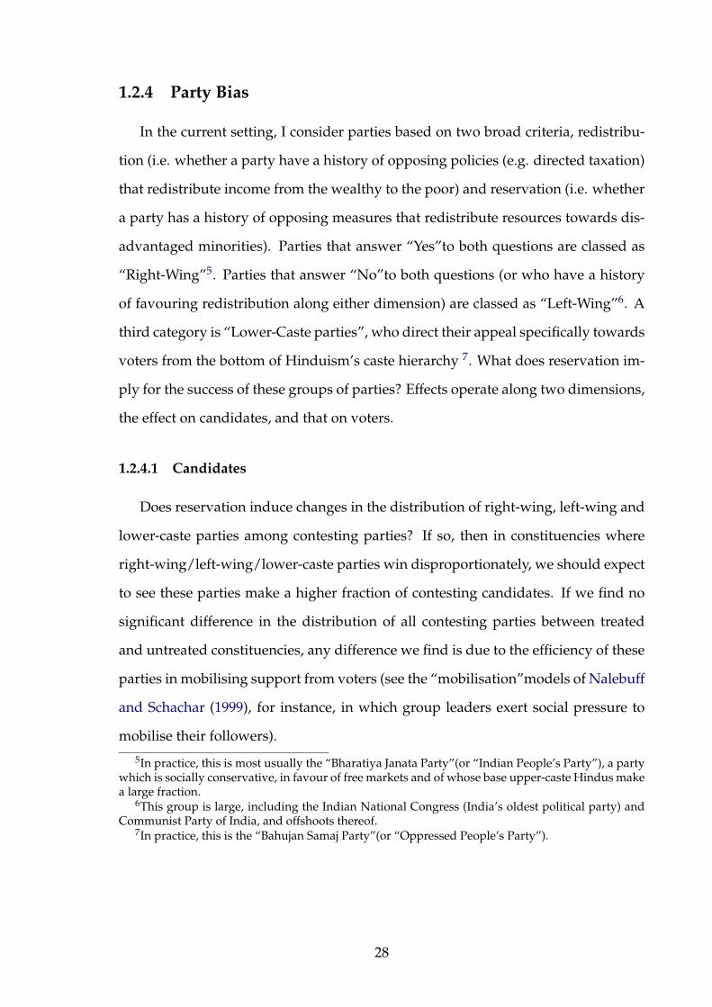
In the current setting, I consider parties based on two broad criteria, redistribu-

tion (i.e. whether a party have a history of opposing policies (e.g. directed taxation)

that redistribute income from the wealthy to the poor) and reservation (i.e. whether

a party has a history of opposing measures that redistribute resources towards dis-

advantaged minorities). Parties that answer “Yes”to both questions are classed as

“Right-Wing”5. Parties that answer “No”to both questions (or who have a history

of favouring redistribution along either dimension) are classed as “Left-Wing”6. A

third category is “Lower-Caste parties”, who direct their appeal specifically towards

voters from the bottom of Hinduism’s caste hierarchy 7. What does reservation im-

ply for the success of these groups of parties? Effects operate along two dimensions,

the effect on candidates, and that on voters.

1.2.4.1 Candidates

Does reservation induce changes in the distribution of right-wing, left-wing and

lower-caste parties among contesting parties? If so, then in constituencies where

right-wing/left-wing/lower-caste parties win disproportionately, we should expect

to see these parties make a higher fraction of contesting candidates. If we find no

significant difference in the distribution of all contesting parties between treated

and untreated constituencies, any difference we find is due to the efficiency of these

parties in mobilising support from voters (see the “mobilisation”models of Nalebuff

and Schachar (1999), for instance, in which group leaders exert social pressure to

mobilise their followers).

5In practice, this is most usually the “Bharatiya Janata Party”(or “Indian People’s Party”), a partywhich is socially conservative, in favour of free markets and of whose base upper-caste Hindus makea large fraction.

6This group is large, including the Indian National Congress (India’s oldest political party) andCommunist Party of India, and offshoots thereof.

7In practice, this is the “Bahujan Samaj Party”(or “Oppressed People’s Party”).

28

1.2.4.2 Voters

Does reservation induce changes in the composition of the voting population in

order to disproportionately favour a group of political parties? If so, then in con-

stituencies where right-wing/left-wing/lower-caste parties win disproportionately,

we should expect to see voters identifying themselves as supporters of right-wing,

left-wing and lower-caste parties (respectively) should make a higher fraction of the

voting population.

Note further that while the above discussion makes no definitive predictions re-

garding the distribution of political parties as a result of reservation, it offers some

suggestive leads as to the composition of the voting population- in particular, it

suggests that uninformed voters may abstain. If a lack of information is also cor-

related with a lack of education or wealth, then when uninformed voters drop out

local elites make a higher fraction of the voting population, which means that if

”informed” voters disproportionately favour a political party, reservation will bias

victory in favour of that party.

1.3 Reservation in India

After 1950, the Indian Government enforced mandated representation for tra-

ditionally under-represented minorities, the Scheduled Castes (SCs) (who belong

to castes at the bottom of Hinduism’s caste hierarchy) and Scheduled Tribes (STs)

(members of which belong to tribes living in remote areas, historically cut off from

technology, education and healthcare). As near as possible, the representation from

each state in State and National Legislative Assemblies would be equal to the pro-

portion of their population in the state, according to the last decennial census. While

the representation of these communities in the population varies continuously, their

representation in the legislature varies with a lag in intercensal years. The fraction of

reservation has remained fixed since the 1981 census. In 2008 the Delimitation Com-

mission of India conducted a revision according to the 2001 census for elections in

29

or after 2008.

When a seat is reserved for a member of the Scheduled Castes (Tribes), only

Scheduled Caste (Tribe) candidates may contest, though all voters on the electoral

roll may vote. From 1962, all constituencies are single-member jurisdictions. Elec-

tions are conducted on a First-Past-the-Post (FPTP) system: the candidate with the

highest number of votes wins and represents the constituency in the state legislative

assembly.

One difference between reservation in the state and national assemblies and that

at the Panchayat (village council) level is that in the former case reserved seats do

not rotate- a seat, once reserved, will remain so as long as it meets the criteria of the

Election Commission.

1.4 Identification Strategy

Quota allocations are determined at three levels: State, District and Constituency.

The hierarchy is as follows: directly beneath the state is a district, which comprises

many constituencies. A district is allocated SC seats in a proportion roughly equal

to how many of the state’s SCs live in that district. Constituencies in a district are

ranked in descending order of proportion of SCs until the district quota is satisfied.

Figure A.1 illustrates the process of allocation of reserved constituencies to a

district. If State X has 15 SC seats and 20% of the state’s SCs live in district A, district

A gets 3 SC seats. Constituencies are ranked in descending order of SC population

until the quota is reached.

Since seats are reserved for minorities based on their representation in the con-

stituency, the identification of reservation on turnout or electoral competition is

not straightforward. However, the procedure described suggests a Differences-in-

Differences approach 8:

8The control group is identified using an approach akin to that of Clots-Figueras (2007) who,examining the impact of female legislators on education expenditure, instruments female presencein administration with females who won elections against men by a narrow majority; Fujiwara (2010)compares the impact of the introduction of Electronic Voting Machines between cities of population

30

1.4.1 Construction of Treatment and Control Groups (SC constituen-

cies)

For each district, I identify the lowest SC proportion for an SC-reserved con-

stituency. This becomes the cutoff for reserved constituencies in each district.

Figure A.2 illustrates the district cutoff in our example. 3 seats were reserved for

SCs in district A, and the lowest SC population among reserved seats was 30%.

I then narrow consideration to constituencies with an SC population within 3

percentage points of the district cutoff: in our example, as illustrated by Figure A.3,

constituencies with an SC population at least equal to 27% and no more than 33%.

I discard constituencies that were previously reserved, since I am interested in

the effects of being reserved for the first time in 2008 (see figureA.4). This leaves me

with the following subgroups: (i) the treatment group, constituencies which were

switched for the first time from nonreserved to SC in 2008 and with an SC proportion

no more than 3 per cent higher than the district cutoff; and (ii) the control group,

constituencies which were never reserved and with an SC proportion no more than

3 per cent lower than the district cutoff.

As in Figure A.5, the treatment group would be: first- time - reserved SC con-

stituencies with an SC population no more than 33 per cent. The control group

would be never - reserved constituencies with an SC population no lower than 27

per cent.

1.4.2 Construction of Treatment and Control Groups (ST constituen-

cies)

The process of allocating quotas to STs is different, since this community is more

geographically concentrated. The state quota for STs is determined similarly to that

for SCs, but constituencies are ranked in descending order of ST population until the

state quota is reached. For this reason, using a similar identification strategy leaves

at least as high as 100000 and cities just below that population threshold.

31

very few observations, so from now on I confine my discussion to reservation for

SCs.

1.5 Empirical Specification

I wish to measure the impact of restricting candidate identity on turnout, the

ratio of candidates to electors, the margin of victory and the probability of success

of right-wing parties. I use a Differences-in-Differences approach, and regress de-

pendent variable Y (turnout, the ratio of candidates to electors, the difference in

voteshare between the winner and runner-up or the probability of success of vari-

ous party groups) on the incidence of being in a constituency reserved for the first

time in 2008 (TREAT), the incidence of being in a year after reservation (POST)

and that of being in a reserved constituency after reservation (TREAT·POST), in

constituency c in year t.

Yct = β0 + β1TREATc + β2POSTt + β3TREATc · POSTt + uct (1.1)

β3 identifies the effect of reservation on turnout, electoral competition and party

bias under the identifying assumption of common trends between treatment and

control groups. In the following section, I test for systematic initial differences be-

tween the treatment and control groups.

1.6 Data

Four states in India carried out elections using the new rules in 2008: Chhatis-

garh, Madhya Pradesh, Karnataka and Rajasthan. Applying the rule described

above leaves me with 107 constituencies for SC constituencies. The four states in

the sample carried out elections in 2003 and 2004. Delimitation in line with the

2001 Census was announced in 2006, so I discount bias owing to prior anticipation

of treatment at least within the sample. The Delimitation Commission of India re-

32

leased detailed documents along with the 2008 announcement, from which I can

reconstruct the reservation of each constituency. This process is not as transparent

for previous rounds of reservation, so I restrict myself to one election year before

and after reservation. Further details on construction of the treatment and control

group are provided in Section C.

1.6.1 Summary Statistics: Village Averages

Table B.1 presents baseline village averages for treated and untreated constituen-

cies, from the 2001 Census of India. There are, on average, 10 villages in each

constituency. As Table B.1 makes clear, constituencies in the treatment and control

groups do not differ significantly across a battery of characteristics including popu-

lation, literacy, employment or fraction of young. Treated constituencies had an SC

population of 21% in 2001 as opposed to 19 % in untreated constituencies. Illiteracy

in to-be-reserved constituencies was 53% in 2001 in both treated and never-reserved

constituencies. Unemployment was 47% in to-be-reserved constituencies and 48%

in never-reserved constituencies.

1.6.2 Summary Statistics: Constituency Averages

Panel A of Table B.2 presents baseline constituency-level electoral characteristics

for treated and untreated constituencies. To-be-reserved constituencies had fewer

candidates from right-wing or centre and centre-left parties among all candidates

contesting the election, but did not differ significantly in the victory rates of left-

wing or right-wing parties9. There are also no significant differences in gender

representation: 5% of all candidates (and 3% of all winners) in to-be-reserved con-

stituencies in 2003 and 2004 were female, versus 6% of all candidates (and 3% of

9In addition to the Communist Party of India and splinter groups, I class India’s oldest politicalparty (The Indian National Congress) and its offshoots as Left/Centre-Left.“Lower-Caste”parties arethose whose manifestoes or rhetoric are directed towards those at the bottom of the caste hierarchy.In practice, this is effectively one party: the Bahujan Samaj Party, or the Party of the OppressedMajority.

33

winners) in untreated constituencies10.

Panel B of Table B.2 presents constituency-level electoral characteristics after

treatment for treated and untreated characteristics. In 2008, to-be-reserved con-

stituencies had fewer candidates from right-wing or left/centre-left parties, but 23%

more winning candidates came from right-wing parties in treated constituencies,

and (unsurprisingly enough) 20% fewer of the winning candidates came from left-

wing parties.

Table B.3 presents constituency-level averages of the dependent variables for

to-be-reserved and never-reserved constituencies. There are no significant differ-

ences between the treatment and control groups prior to reservation over any of

the dependent variables. Turnout in 2008 was seven percentage points lower in re-

served constituencies compared to never-reserved constituencies. Right-wing can-

didates made 63% of winners in constituencies reserved in 2008, versus 41% in

never-reserved constituencies. The bottom panel presents differences in differences

for the four dependent variables. The change in turnout was six percentage points

lower in reserved constituencies. The share of right-wing winners rose by 11% in

reserved constituencies, and fell by 16% in never-reserved constituencies.

We might be concerned that the differences-in-differences that we observe with

the victory of right-wing candidates are driven entirely by changes coming from the

control group, rather than the treatment group. However, right-wing candidates

made up 2% fewer of winning candidates in all SC constituencies moving from 2003

or 2004 to 2008; 26% fewer of all winning candidates in ST constituencies, and 5%

fewer of all winning candidates in all nonreserved constituencies. Right-wing par-

ties, therefore, were less successful in 2008 than in 2003 or 2004 everywhere but in

to-be-reserved constituencies.10It is possible that to-be-reserved constituencies would have significantly more or fewer minority

candidates. Unfortunately, the SC/ST status of candidates in unreserved constituencies only appearsin the data from 2004. The state of Karnataka has caste data for candidates from 2004 onwards. 9%of candidates in to-be-reserved constituencies were SCs, versus 5% in never-reserved constituencies.The difference is not significantly different from zero.

34

1.7 Results: Aggregate

1.7.1 Basic Results

In Table B.4 I present the results from estimating equation 1.1. From Panel A of

column 3 of Table B.4, turnout in reserved constituencies after treatment drops by 6

percentage points relative to a baseline of 69 percentage points i.e. turnout falls by

9%. This result is robust to district fixed effects and a set of controls including aver-

age female literacy in 2001 and average 2001 unemployment. Turnout is positively

correlated with the POST dummy i.e. being in a year after treatment, but the effect

is small and the partial effect of reservation is still large, negative and significant.

As we see from columns 3 and 4 of Panel B of Table B.4, being in a reserved con-

stituency after treatment has a positive correlation with the ratio of candidates to

electors: being in a reserved constituency after reservation causes the ratio of candi-

dates to electors to rise by 8%. The effect is not precisely estimated, but reservation

has no discernible negative impact on this measure of electoral competition.From

Panel C of Table B.4, being in a treated constituency after reservation is positively

correlated with the margin of victory: the point estimate is 3 percentage points rel-

ative to a baseline of ten percentage points. However, the effect is imprecisely es-

timated11. As we see from Panel A of Table B.5, the probability that the winning

candidate is from a right-wing party is 26% higher in a reserved constituency after

reservation. Suggestively, the probability of victory of ”lower-caste” parties is lower

in the treated sample after treatment (as we see in Panel C), but the effect cannot be

disentangled from mean reversion.

There is also the question of exit: to argue that reservation causes turnout to

drop, we ought also to consider the reverse: whether turnout rises when a con-

stituency always reserved for SCs gets unreserved. Table B.6 considers constituen-

11As I outlined earlier, owing to their concentration, the sample of constituencies that are narrowlyreserved or left unreserved for STs is very small, so the presence or absence of effects is difficult toargue. However, while widening the cutoff to 5 or 10 percentage points has no large impact on thesize of the effect of SC reservation on turnout, the point estimates of the difference-in-difference inST constituencies (not reported) is consistently small and not significantly different from zero

35

cies unreserved (with control group identified as in Section 1.4), and shows that

turnout rises by 4 percentage points (relative to a baseline of 67 percentage points).

The ratio of candidates to electors rises by 43% (whereas in constituencies newly

reserved for SCs, the impact on this measure of electoral competition is not different

from zero), while, as with constituencies newly SC-reserved, dereservation is not

associated with a significant change in the margin of victory.

The bottom panel considers the fraction of winning candidates coming from

right-wing, left-wing and lower-caste parties in constituencies newly reserved and

newly-unreserved. While right-wing candidates make up a significantly higher frac-

tion of winners in newly-reserved constituencies, no group seems to win signifi-

cantly more often in newly-unreserved constituencies.

1.7.2 Robustness Checks

In this section I consider relaxing some of the restrictions in my specifications.

Currently, constituencies are categorized as treated or untreated if their SC popu-

lation is within 3 percentage points above or below the district cutoff described in

Section 1.4; the choice of specification leaves room for the possibility that some dis-

tricts will have only treated or untreated constituencies. Further, there are concerns

endemic to work using Difference-in-Difference specifications: serial correlation of

standard errors, prior trends and possible endogeneity of treatment (Bertrand, Du-

flo, and Mullainathan (2004)). The dependent variables that I examine (turnout,

electoral competition and the probability of success of right-wing parties) are quite

likely highly subject to serial correlation. However, in my data at present the time-

series dimension is less likely to be an issue: for each constituency, I consider the

election period prior to reservation, and the election year after reservation. The

method of selection of control groups also indicates that endogeneity of treatment

is less likely to be a concern. Furthermore, work examining Delimitation indicates

that constituency boundaries, where redrawn, were done so solely in order to en-

sure equal electorate sizes, with no evident bias, partisan or otherwise (Iyer and

36

Shivakumar (2009)). This leaves the matter of prior trends.

1.7.2.1 Placebo Checks

Table B.7 presents results for turnout, the ratio of candidates to electors and the

margin of victory for the sample, but as though reservation were carried out in 1998

rather than 2008. Since for 5 constituencies no analogue exists prior to 2001, I present

my main results with and without these constituencies (columns 1 and 2 respec-

tively). Column 3 runs a placebo for the main specification and illustrates that being

in a treated constituency after 1998 has no significant impact on turnout or electoral

competition. This may go some way toward allaying concerns of prior trends.

Table B.8 indicates that the results suggesting that right-wing parties win dis-

proportionately often in newly-reserved constituencies is not echoed in the sample

constituencies with a placebo treatment carried out one decade prior to reservation.

1.7.2.2 Widening the sample

The results in Table B.4 are also robust to widening the sample to include hitherto-

unreserved constituencies with an SC population within 5 percentage points of the

district cutoff(see B.9) 12.

1.7.2.3 Districts with both Treated and Untreated Constituencies

In Table B.10, I restrict the sample to only districts which have both treated and

untreated constituencies. This constraint, perhaps unsurprisingly, is hard on the

data: almost half the observations are lost, leaving 120 observations. The main re-

sults are left unaffected, however: turnout falls by 5% in reserved constituencies

after reservation, and the ratio of candidates to electors is positively correlated with

being in a reserved constituency after reservation. So, too, is the margin of victory,

but the point estimate is small and the impact is not significantly different from zero

(see B.10).

12I am left with very few observations if I tighten the sample to only those constituencies within 1percentage point of the district cutoff. However, the magnitude of effect is very similar.

37

1.8 Individual-level Voting

In this section I present individual post-poll survey data for 15 constituencies in

one state in the sample. In 2008, an organisation called Lokniti carried out surveys

for a random selection of constituencies after the 2008 State Legislative Assembly

Elections, on behalf of the Centre for the Study of Developing Societies (CSDS). Re-

spondents were asked whether they voted in the most recent legislative assembly

elections (in 2008), whether they voted in the prior elections (in 2004), as well as

about current literacy, asset ownership, gender and ethnic group (religion, subcaste

and classification into SC, ST or otherwise).

Karnataka has 224 constituencies in the state legislative assembly, of which Lokniti

polls 75. Within these constituencies, I look for those meeting the criteria specified

in 1.4. This leaves me with 15 constituencies, of which 6 were reserved for the first

time in 2008, and 9 remain unreserved.

I regress the probability of voting (VOT) for individual i in constituency c in year

y on the incidence of being in a constituency reserved in 2008 (RE) after reservation

(POST) and their interaction; and the effect of being female and/or a minority and

being in a reserved constituency after treatment (ID·RE·POST). I estimate the fol-

lowing equations (in spirit very similar to the previous specification):

VOTicy = α0 + α1REc + α2POSTy + α3REc · POSTy + eicy (1.2)

VOTicy = β0 + β1REc + β2POSTy + β3REc · POSTy + β4 IDic + (1.3)

β5 IDic · REc + β6 IDic · POSTy + β7 IDic · REc · POSTy + uicy

38

1.8.1 Summary Statistics for Lokniti Constituencies: Respondent

Characteristics in 2008

I filter out respondents who cannot remember whether they voted in 2008 or

2004, as well as respondents who were too young (or otherwise ineligible) to vote in

2004 or 2008. This leaves me with 405 respondents from treated constituencies, and

497 from untreated constituencies. As we see from Table B.11, untreated and treated

constituencies do not vary significantly across a range of respondent characteristics:

the fraction of SC respondents in treated constituencies is 16% and 15% in untreated

constituencies; the fraction of all sizable minorities (SC/ST/Muslim/Christian) is

29% in treated constituencies versus 33% in untreated. Women make up 49% of

respondents in treated constituencies versus 42% in untreated constituencies (not

significantly different at 10%). Literacy, monthly income and assets ownership too

did not vary significantly across treated and untreated constituencies. One-fifth of

those polled in untreated constituencies (16% in treated constituencies) responded

“Never”to the questions “How often do you read the newspaper?”;“How often do

you listen to the news on radio?”and “How often do you watch the news on televi-

sion?”, but the difference between treated and untreated constituencies was small.

Since we are left with 6 reserved and 9 unreserved constituencies, it is difficult

to argue that there are or are not systematic differences between the treated and

control group. However, village-level averages from the 2001 Census (out of 1420

villages across treated constituencies and 1827 in untreated constituencies) indicate

that to-be-reserved constituencies have an SC population of 25% as opposed to 21%

in untreated constituencies (see Table B.12), and an ST population of 6% versus 8%

in untreated constituencies, but the difference is not significant. The only charac-

teristic which varies significantly across treatment and control groups is the female

population, and even there the difference is small: 50% in treated versus 49% in

untreated constituencies. Similarly, since the number of candidates is small for this

reduced sample, it is difficult to confidently argue that the groups are or are not

identical. As Table B.13 indicates, reservation leaves 52 candidates in constituencies

39

reserved in 2008, 59 for those remaining unreserved. It should be noted, though,

that 7 candidates out of 52 in to-be-reserved constituencies were SC, versus 3 out of

59 in never-reserved constituencies. The fraction of candidates from various party

types does not vary considerably across treatment and control groups.

1.8.2 Results: Individual Voting Data

Table B.14 presents results for the Linear Probability Model and Probit estimates

of equation 1.2 to 1.313. From column 2 , it appears that the probability of voting

falls in reserved constituencies after reservation relative to the baseline, by about

4% on average, although the effect is imprecisely estimated. From columns 4 and 5,

we see that female voters are 13% (in the Probit specification) to 15% (in the LPM

specification) less likely to vote in reserved constituencies after treatment relative

to the baseline. Columns 6 to 9 each have different definitions of the term ”minor-

ity”. Columns 6 and 7 examine the impact of being an SC or another minority and

interacting that with the incidence of being in a reserved constituency after reserva-

tion, and columns 8 and 9 lump together any individual who is not an upper-caste

Hindu. Minorities are between 9% (as in columns 8 and 9) and 20% (as in columns 6

and 7) less likely to vote in reserved constituencies after treatment, with the baseline

group of local elites showing no significant change in voter participation. Columns

10 to 13 discuss the effects of controlling both for being female and in a reserved con-

stituency after treatment, and belonging to a minority group and being in a reserved

constituency after treatment. The base group (of male elites) shows no significant

difference in voter participation, while being female reduces voter participation by

about 15% relative to the baseline, and belonging to a minority community reduces

voter participation between 10% (as in columns 12 and 13) and 20% (as in columns

10 and 11).

The data used is taken from a survey in 2008 asking only one retrospective ques-

13Since reservation is at the constituency level, and there are only 15 constituencies in the sample,clustering standard errors at constituency level seems problematic. However, the following resultsare qualitatively very similar using robust standard errors or a block bootstrap approach. I presenthere the most conservative of my observed results.

40

tion. This is not so much a concern for intrinsic characteristics such as gender or

ethnic group, but controls such as monthly income, asset ownership and years of

education do vary over time. However, it seems reasonable to assume that a re-

spondent who was illiterate in 2008 was similarly so in 2004. Columns 14 and 15 of

table B.14 suggest that illiterate respondents in treated constituencies in 2008 were 5

% less likely to vote. The effect, however, is imprecisely estimated.

Columns 16 and 17 of table B.14 suggest that uninformed respondents (who re-

sponded ”never” to how often they consumed news in various media) in treated

constituencies in 2008 were not significantly less likely to vote than informed coun-

terparts. However, respondents were asked about their information acquisition in

2008 only.

1.8.3 Magnitude of Effects

“Back-of-the-envelope”calculations suggest that in the Probit estimation (speci-

fication as in column 5), the predicted probability that the base group of males votes

in a reserved constituency after reservation is 94%, whereas that of females is 72%.

Using a similar procedure, we see that being in an SC constituency immediately

after reservation does not affect the participation of the base group of elites, while

being a minority lowers participation by 14% (columns 7 and 9). In column 11, be-

ing female in a treated constituency after treatment reduces an agent’s probability

of voting by 18%, and the reduction is by 19% in column 13. In column 13, being a

minority reduces voter participation in a treated constituency after treatment by 9%

and in column 11, by between 9% and 12%. Controlling for being a minority in a

treated constituency after treatment, being female reduces participation by between

30% and 32% in column 11 and 31% in column 13. Controlling for being female

in a treated constituency after treatment, being a minority reduces voter participa-

tion by between 26% and 30% in column 11 and 22% in column 13. From Table B.14,

one sees that these magnitudes are qualitatively similar to (though usually bounded

below by) those in the LPM specifications.

41

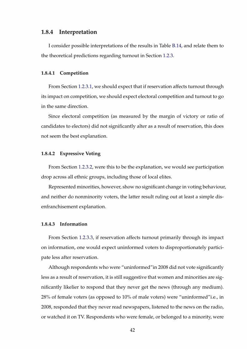
1.8.4 Interpretation

I consider possible interpretations of the results in Table B.14, and relate them to

the theoretical predictions regarding turnout in Section 1.2.3.

1.8.4.1 Competition

From Section 1.2.3.1, we should expect that if reservation affects turnout through

its impact on competition, we should expect electoral competition and turnout to go

in the same direction.

Since electoral competition (as measured by the margin of victory or ratio of

candidates to electors) did not significantly alter as a result of reservation, this does

not seem the best explanation.

1.8.4.2 Expressive Voting

From Section 1.2.3.2, were this to be the explanation, we would see participation

drop across all ethnic groups, including those of local elites.

Represented minorities, however, show no significant change in voting behaviour,

and neither do nonminority voters, the latter result ruling out at least a simple dis-

enfranchisement explanation.

1.8.4.3 Information

From Section 1.2.3.3, if reservation affects turnout primarily through its impact

on information, one would expect uninformed voters to disproportionately partici-

pate less after reservation.

Although respondents who were “uninformed”in 2008 did not vote significantly

less as a result of reservation, it is still suggestive that women and minorities are sig-

nificantly likelier to respond that they never get the news (through any medium).

28% of female voters (as opposed to 10% of male voters) were “uninformed”i.e., in

2008, responded that they never read newspapers, listened to the news on the radio,

or watched it on TV. Respondents who were female, or belonged to a minority, were

42

uninformed by this definition 26% of the time, whereas male nonminority respon-

dents were only uninformed 12% of the time, the difference statistically significant.

If candidate ethnic group is a proxy for information about candidate characteris-

tics,it is quite possible that if all candidates share the same broad ethnic group, a

major source of information is lost.

1.9 Conclusion

This paper joins the debate on the merits of political reservation with a note on

its impact on political participation and electoral competition, and does not support

claims that mandated minority representation reduces competition. However, voter

participation drops in constituencies with restricted candidate identity. Evidence

from a subsample indicates that mandated minority representation may reduce par-

ticipation for women and for minority groups.

Further work will consider testing for common trends using previous Census

data for the sample constituencies. It would also consider sample extension, since

five other states carried out elections in 2011. Four of these states are the populous

Assam, Tamil Nadu, Kerala and West Bengal. The wider sample (once released)

may enable us to observe the impact of reservation of constituencies for Scheduled

Tribes, a task so far rendered impossible by the limitations of the existing sample.

In addition, the most recent round of delimitation took place in 2008, so I can only

observe constituencies immediately after treatment, and for one election year im-

mediately prior to treatment. Further work would examine whether the impact on

turnout that I observe continues. Lastly, a theoretical extension might look at the im-

pact of electoral systems: for instance, how does the First-Past-the-Post FPTP system

affect this outcome, as opposed to Proportional Representation?

43

Chapter 2

Why do Workers Remain in

Low-Paying Hereditary Occupations?

2.1 Introduction

Occupational rigidity has appeared in various forms all over the world, from

guilds in Mediaeval Western Europe to the caste system in India. These systems

differ along several dimensions, but they share the following features: recruitment

into occupations happens early (in the case of the caste system, at birth) and workers

remain in hereditary occupations, even when pay is low.

The case of the Indian caste system in particular has received a great deal of at-

tention, not least because of its persistence. Many persuasive theories have been

propounded to explain intergenerational occupational rigidity, ranging from the

difficulty of acquiring the human capital required to switch jobs (Bannerjee and

Newman (1993)), to the role of caste groups in minimizing information asymmetries

(Akerlof (1976), Greif (1993)) and thus lending themselves to contract enforcement

(Freitas (2006)) or social insurance (Munshi and Rosenzweig (2009)).

This paper suggests that, in environments with limited or no contract enforce-

ment or insurance provision, occupational (or spatial) mobility is limited by the

insurance-provision function of networks- in the case of this paper, that of the fam-

ily. While occupational specialization by community (the caste, or jati1, in India, in

1The jati refers to a subcaste rather than a caste, which is usually considered the relevant unit inthe literature.

44

particular) has been studied before (Akerlof (1976), Akerlof (1980)), this paper sug-

gests that insurance can generate intergenerational occupational rigidity(which is

frequently conjectured (Freitas (2006)) or assumed (Greif (1993)), but so far has not

been explicitly derived), as well as occupational specialization.

I use a two-period Overlapping Generations model in which a parent with an

endowment of occupation-specific human capital transfers costly human capital to

her offspring, in return for full insurance if the parent suffers an accident. If the off-

spring participates in the arrangement and insures her parent in case of an accident,

she can use the human capital passed on to her by her parent in the final period of

her life. If she defaults, she cannot use this and she and her descendants are barred

from the insurance arrangement.

I find that agents with low levels of human capital are more likely to participate

in the insurance arrangement, since their costs of training their offspring are lower.

As the cost of sickness rises, parents are willing to disseminate higher amounts of

specific human capital, and the highest sustainable human capital transfer rises with

the cost of sickness.

This paper unites two broad views of caste: a “functional”view, suggesting that

guilds, castes or professional associations are designed to protect intellectual prop-

erty or rents of any kind, and that of castes or trading associations as a corrective

of information-related market failures. The existing literature on castes as contract-

enforcement mechanisms or insurance providers tends to ignore this role, but there

is considerable evidence that castes functioned as professional associations. For one

thing, as with guilds, many caste surnames reflect ancestral occupations. Castes

were largely ascriptive as early as 303 B.C. (Blunt (1969)), and Indian mythology

contains several intriguing accounts of the role of the divine order in protecting pro-

prietary knowledge. For instance, one account of the first of the ten incarnations

of the preserver, Vishnu, begins with the theft of metaphysical knowledge from the

mouth of a sleeping Creator. The preserver, Vishnu, must retrieve the knowledge

before those who are not entitled to it can use it.

45

This paper complements an extensive literature on occupationally-specialized

networks, from studies of the guild economy in mediaeval and early modern Eu-

rope (Ogilvie (2004)) to Colonial and modern India (Buhler (1886)), (M.N.Srinivas

(1962)). The Indian caste system has attracted much attention owing to its central-

ity in Indian politics (some of which is addressed in Chapter 1), the range of forces

used to change it, either legislative or economic, and its resilience in the face of these

forces.

Recent work by Banerjee, Bertrand, Datta, and Mullainathan (2009) examines

labour-market discrimination in the technology industry on the basis of caste and

religion, and finds no significant evidence of discrimination against lower-caste ap-

plicants. Bertrand, Hanna, and Mullainathan (2010) find that affirmative action in

education does not seem to adversely affect the perception of beneficiaries. How-

ever, endogamy seems to be more stubborn: Banerjee, Duflo, Ghatak, and Lafortune

(2009) show that a preference for partners of the same community persists even de-

spite urbanisation and economic growth.

There has long been an interest in the benefits of seemingly autocratic and in-

efficient institutions- from labour market access (Munshi and Rosenzweig (2006),

Luke and Munshi (2006)) to access to credit and insurance (Munshi and Rosen-

zweig (2009), Townsend (1994), Chiappori, Samphantharak, Schulhofer-Wohl, and

Townsend (2011), Berman (2000)). A key part of these benefits comes from the role

of networks in enforcing co-operation absent formal contract enforcement (Akerlof

(1976), Akerlof (1980), Freitas (2006) and Greif (1993)). See also the literature on

group lending with joint liability (Ghatak and Guinnane (1999), Ghatak (1999)).

It has also been understood that contractual responsibilities can be passed inter-

temporally, from generation to generation (for instance, Eswaran and Kotwal (1985)

indicates that labour contracts pass from father to son). While discussing the Maghribi

mercantile trading association of the mediaeval Middle East, Goitein (1973) observes

that sons followed their father’s occupations, and further defaults or obligations

were transferred to relatives or offspring (Goitein (1978)).

46

This paper belongs to the broader literature on the persistence of archaic insti-

tutions, with a particular emphasis on the relationship between dynastic human

capital and the provision of insurance.

The remainder of the paper is organized as follows. Section 2.2 provides some

brief background regarding hereditary occupations and the caste system, as well as

the Indian “joint family”(in which an extended family lives under the same roof)

and norms dictating parental care. Section 2.3 considers alternative explanations of

the phenomenon of extended families. Section 2.4 provides a simple model of in-

surance in which an agent transfers costly human capital to her offspring in return

for insurance in the event of an accident. Section 2.4.2 derives predictions for the

maximum human capital transfer that a parent is willing to make, and Section 2.4.3

shows the child’s problem, with Section 2.4.3.1 deriving predictions for the mini-

mum human capital transfer that a child is willing to accept for an interior solution.

Section 2.5 shows results for a numerical simulation of the baseline model. Section

2.6 concludes with some ideas for further work.

2.2 Background

2.2.1 Caste in India: Ascriptive or not?

The word ”caste” comes from the Portuguese word ”casta”, meaning mould,

breed or race. The definition of what constitutes a ”caste” has mutated consider-

ably, but for the most part it is taken to mean an endogamous group of people who

observe (with varying degrees of strictness) rules pertaining to food, drink, work

(on which more later) and association with each other and those of other groups.

There is some doubt as to whether castes were designed primarily as units of

occupational specialization. Rules 96-99 of Chapter X of the Laws of Manu (Buh-

ler (1886)) are explicit about the dangers of assuming the functions of those castes

higher than one’s own: “A man of low caste who through covetousness lives by the

occupations of a higher one, the king shall deprive of his property and banish. It

47

is better (to discharge) one’s own (appointed) duty incompletely than to perform

completely that of another; for he who lives according to the law of another (caste)

is instantly excluded from his own”.

However, rules 80-95 suggest that there is some latitude, provided that certain

“polluting”occupations are avoided. “Among the several occupations the most

commendable are, teaching the Veda for a Brahmana, protecting (the people) for a

Kshatriya, and trade for a Vaisya. But a Brahmana, unable to subsist by his peculiar

occupations just mentioned, may live according to the law applicable to Kshatriyas;

for the latter is next to him in rank. If it be asked, ’How shall it be, if he cannot

maintain himself by either (of these occupations?’ the answer is), he may adopt a

Vaisya’s mode of life, employing himself in agriculture and rearing cattle. But a

Brahmana, or a Kshatriya, living by a Vaisya’s mode of subsistence, shall carefully

avoid (the pursuit of) agriculture, (which causes) injury to many beings and de-

pends on others..... If he applies sesamum to any other purpose but food, anointing,

and charitable gifts, he will be born (again) as a worm and, together with his ances-

tors, be plunged into the ordure of dogs. By (selling) flesh, salt, and lac a Brahmana

at once becomes an outcast; by selling milk he becomes (equal to) a Sudra in three

days. But by willingly selling in this world other (forbidden) commodities, a Brah-

mana assumes after seven nights the character of a Vaisya.... A Kshatriya who has

fallen into distress, may subsist by all these (means); but he must never arrogantly

adopt the mode of life (prescribed for his) betters”.

However, occupational specialization and intergenerational occupational rigid-

ity are frequently associated with castes, and there is considerable evidence that

castes functioned as professional associations, in which recruitment happened at

birth. Blunt (1969) notes that Megasthenes, on a visit to India in 303 B.C, observed

that “No one is allowed to marry out of his own caste, or to exchange one profession

or trade for another, or to follow more than one business”.

48

2.2.2 The Joint Family

Almost three quarters of all the rural elderly in India live with their children, and

it is understood that responsibility for the care of an ailing and aged parent falls to

the child. Karve (1953) suggests that even in 1000 B.C., the joint family (”a group of

people who generally live under one roof, who eat food cooked in one kitchen, who

hold property in common, participate in common family worship and are related to

one another as some particular type of kindred.”) existed in a similar form to that

understood today. Members of the same extended family frequently live in the same

residence. Karve (1953) notes that parents lived with married sons, and up to four

generations lived under the same roof.

2.2.2.1 Filial Responsibility

Cultural norms dictate that responsibility for caring for the elderly parent rests

with the (usually male) child. Primary Vedic texts state, for instance, ”Matru Devo

Bhava”, ”Pitru Devo Bhava”, which mean ”venerate your mother and father as you

would God”. Chapter 8 of the Mahanirvana Tantra (or ”Spiritual System of Great

Liberation”), from a translation by Woodroffe (1976) states that “The man who, to

the deprivation of his elders ....., fills his own belly is despised in this world, and

goes to Hell in the next”; “He who becomes an ascetic, leaving mothers, fathers,

infant children, wives, agnates and cognates, is guilty of a great sin”; “The body is

nourished by the mother. It originates from the father. The kinsmen, out of love,

teach. The man, therefore, who forsakes them is indeed vile”.

In Chapter III of the Laws of Manu (translation by Buhler (1886)) is prescribed

the banning from sacred rituals ”he who forsakes his mother, his father or teacher”

(Rule 157) and ”he who wrangles or goes to law with his father” (Rule 160). Further,

in Chapter XI, the sins leading to a loss of caste include ”casting off ones teacher,

mother, father, or son.... selling... one’s wife, or child... casting off a relative”. This

is a serious penalty, as it means not only social ostracism for the offender, but also

an inability to practise his occupation.

49

There were also sanctions against travel, particularly foreign travel. Interest-

ingly these seemed to apply to agents from higher rather than lower castes. Hutton

(1961) notes that ”One restriction on Hindus.....applies, or used to apply, with much

greater force to higher than to lower castes, and that is the prohibition against going

overseas”. Insofar as high-caste agents may be said to have higher human capi-

tal than lower-caste agents, this may reflect stronger attempts to preclude parental

abandonment by children with substantial human capital.

2.2.2.2 Parental Responsibility

On parental duties Chapter 8 of the Mahanirvana Tantra says of the householder:

“A father should fondle and nurture his sons until their fourth year, and then until

their sixteenth they should be taught learning and their duties”. This rather milder

injunction seems born of greater anxiety regarding filial misbehaviour than that of

parents. One explanation for this is that parents are altruistic towards children and

not vice versa, and another is that children could commit less to caring for parents

than the other way around.

In the following section, I lay out a simple model of insurance in which agents

accumulate human capital to transmit to their offspring in return for care in the

event of sickness. But first I consider in more detail some alternative explanations

of the phenomenon of filial responsibility for parental care in developing countries.

2.3 Altruism, Asset Poverty or Insurance

One simple explanation for the coresidence of elderly parents with children is

that of altruism: i.e. parents wish to maximize their children’s utility and children

care about their parent’s utility. However, were this the case, it is difficult to explain

retention of children in low-paying hereditary occupations2. Moreover, there are

documented instances of recent abandonment of or cruelty towards aging parents,

leading the Parliament of India to pass the “Maintenance and Welfare of Parents2It is also tempting to suggest that there would be no need for specific prescriptions regarding the

care of kin if children or parents looked after each other without prompting.

50

and Senior Citizens Act”in 2007, which creates provisions for the punishment of

children who abandon or neglect parents dependant on them.

Another persuasive explanation frequently offered is that of asset-poverty in the

presence of indivisible human capital investments and capital market imperfections

a la Bannerjee and Newman (1993) i.e. parents and children cannot afford to invest

in the human capital necessary to move out of traditional occupations. However,

there is evidence indicating that even when parents can afford to give a child costly

education, the child expected to care for the parent still remains in the traditional

occupation.

2.3.1 Traditional Occupations and Parental Reponsibility

As Munshi and Rosenzweig (2006) show in a study of occupational choice by

gender in a community in Western India, it was male children who received net-

work benefits and were discouraged from seeking occupational choices that would

weaken the network, and who thus could not benefit from the increased return

to outside occupational choices, even when the parents could afford to send their

daughters to costlier schools with higher wage returns to education.

Part of the common wisdom behind a preference for sons in developing coun-

tries like China and India is that responsibility for caring for elderly parents lies with

sons, whereas daughters cannot be relied on to look after aged parents (the scrip-

tural prescriptions described earlier apply specifically to male householders.). The

phenomenon was also observed elsewhere: while discussing the Maghribi mercan-

tile trading association of the mediaeval Middle East, Goitein (1973) observes that

fathers regarded sons as their “insurance policies”. In India, 60% of elderly people

live with male children 3.

Thus asset poverty alone cannot explain why children are retained in low-paying

hereditary occupations. This suggests a form of intertemporal exchange, in which

3Karve (1953) points out that in the south Indian state of Kerala, we observe that married womenlive with their mothers. We will consider the phenomenon observed in other Indian states of kinshipthrough male ancestors.

51

dynastic capital is transmitted to the child expected to care for the elderly parent4.

2.3.2 Family, Caste and Insurance

Finally, in India, especially in rural areas, family networks are still the largest

source of insurance (Munshi and Rosenzweig (2009))- informal loans from family

members make up a higher fraction of loans than from friends or employers. A

commonly cited reason for this is that caste or jati networks have informational

advantages- I.R.Dave (1976) says of a premodern Indian trading association “[They

were] very keen to stick to truth in their dealings”. Further, they “seldom bor-

row[ed] from other than their castemen”(A.J.Saunders (1920–1922)). Hutton (1961),

when describing the functions of caste, says that “[an individual caste member’s

caste] acts as his trade union, his friendly or benefit society, his health insurance,

and if need be provides for his funeral”.

There is extensive anecdotal evidence suggesting that members of the same caste

were in an excellent position to know each other’s doings either through frequent

social interaction or by living with or in close quarters to each other. Members of

the same jati traditionally lived in close quarters. As E.R.Leach (1960) notes, ”The

Brahmans exhibit a high degree of internal interaction and external exclusiveness.

As kinsfolk, they invite each other to feasts... initiations, marriage, death and ances-

tral rites.. Houses are built with walls adjoining; holes in the walls permit women

to pass messages to each other. Children are socialized within the street and until

the age of five do not mingle with those of other castes”.

Assuming that information flows more effectively in small communities, one

should expect that (i) as the size of a caste increases, it should split in order to more

effectively monitor its members and (ii) as families increase in size, they should split

into different units. In Freitas (2006) one sees for South Indian castes between 1823

and 1941 that there is a positive correlation between the number of distinct jatis and

population size. Anthropological surveys from Karve (1953) suggest that as family

4This implies, in turn, that if a parent had more than one son the son expected to care for theparent would be likelier to receive ancestral capital.

52

sizes increase, extended families split and move into different residences. ”Every

existing joint family is a piece broken off from a larger unit.” ”the northern family

often breaks up at the death of the man who first founded it. When such a family

splits and there is partition....into smaller joint families made up of a man, his wife

and children , son’s sons and daughters; or a man, his wife and children and a

couple of younger brothers who wish to have his protection or who may not be old

enough to take care of themselves.”

Rural justice frequently devolves upon Caste Councils or Jati Panchayats, who

were observed to have an excellent sense of the truth of matters. Hutton (1961)

says that “Caste panchayats [councils] will generally be very much more likely to

know the true facts of offences their castemen have committed than the ordinary

law courts are”. He also notes the importance of small localities in the transmission

of information: “The caste council can only act for a limited area, an area small

enough ... for members of the caste within the area to have some knowledge of each

other as a general rule”. Blunt (1969) observes something similar: “There is not one

panchayat only to each endogamous group, but one panchayat to each independent

local section of the group”.

It seems reasonable to expect, thus, that the dynastic capital transmitted to the

child is frequently tied to a specific location, where the social network can relay

information about its members.

I propose an explanation that ties together the following observed phenomena:

(i) hereditary occupations- specifically those where male offspring use the family’s

dynastic capital; (ii) coresidence of parents with sons; (iii) the informational advan-

tages of local, occupationally specialized networks. How did parents induce their

children to remain nearby in order to smooth consumption when older? By provid-

ing them with training that would be useless if they travelled far away, or remained

in the same area without abiding by the terms of the social contract.

To this end, I derive a simple model of insurance in which agents keep children in

hereditary occupations by passing on human capital, and in which children remain

53

in hereditary occupations so as to have specific human capital to pass on.

2.4 Model

It is difficult, when drawing on historical records, sociological documents and re-

ligious law to make inferences about social practice, to judge the use of assumptions.

Does the author stick to only those are assumptions which are directly borne out by

the text, or may she use those which are not directly contradicted by her sources?

Similarly, how is she to use historical record when evaluating her findings?

I will use anecdotal evidence from historical records or anthropological surveys

to either back up assumptions (and attempt to make as few as possible assumptions

that do not seem directly indicated by accounts of common practice), and to support

the claims that I make. A note on my use of scriptural sources: I will frequently be

using the existence of prescribed sanctions or punishments in scripture not only as

evidence that such activities carried a cost if discovered, but also as evidence that

agents had an incentive to misbehave without the threat of a punishment.

2.4.1 Model Setup

In this model, each agent lives and consumes in two periods of life: Child (C)

and parent (P). In the first period, the child works for her parent, who gives the

child costly human capital which is only valuable if used locally, in return for full

coverage if the parent is sick. If the child insures her parent, she can use her human

capital as a parent to get insurance from her child. If she does not insure her parent,

she is not allowed to use her human capital by the network of practitioners of the

same occupation; thus, her human capital is worthless. Further, she is not permitted

to use the insurance arrangement.

The model is timed as follows: in Period 1, the parent transfers costly human

capital to the child. After the parent makes her choice of human capital transmis-

sion, she and her child find out whether the parent is sick and (if the parent chose

insurance) the child decides whether to make a transfer to the parent. The parent

54

dies at the end of Period 1.

At the beginning of Period 2, the child is now a parent with her own child. If

the parent was sick at the end of Period 1, it is revealed whether the child insured

the parent honestly. If she did, she is allowed to use her human capital, and must

choose whether to seek insurance by transmitting h′′ to her own child, or autarky.

If not, she is not allowed to practise the occupation in which she was trained, and

is barred from the insurance arrangement. Then the child discovers whether she is

sick, and if she has chosen insurance her offspring must choose whether to insure

her. The child dies at the end of Period 2.

In each period, the parent has a probability of sickness π. This π is drawn inde-

pendently in each period. If the agent is sick she incurs a disutility I. If the parent

chooses not to get insurance she has the use of the entirety of her human capital f (h).

If she chooses to get insurance, the parent with human capital f (h) transfers to her

child human capital h′ with time cost c(h′), yielding human capital worth f (h′) to

the child. Thus the parent is left with f (h)(1− c(h′)). This time cost captures the

idea that training cost increases in not only the value of human capital imparted to

the child, but also in the value of the parent’s own human capital, which suggests a

motive for retention of workers in low-paying occupations.

If the parent does not fall sick the child has the use of human capital f (h′) in

Period 1 and in period 2. If the parent falls sick and the child insures her parent,

she makes a transfer θ I when the parent falls sick, leaving the child with f (h′)− θ I.

θ < 1 i.e. the child’s cost of caring for the parent is increasing in, but lower than, the

parent’s disutility from sickness. If the child insures her parent, she has the use of

human capital f (h′) in Period 2, otherwise, she cannot practise the occupations in

which she was trained and her human capital is worth 0.

A key assumption here is that information flows perfectly within the family, and

further that practitioners of the same occupation know with certainty whether the

child insured or cheated the parent. This seems reasonable- as Hutton (1961) and

others have stated, the jati or biradari possessed accurate information as to the rights

55

and wrongs of a matter, and of each other’s concerns.

The assumption that the child cannot practise her occupation and remain in the

area is suggested by the practice of outcasteing unfilial children (Buhler (1886)). As

mentioned before, the penalty of outcasteing was indeed the prescribed one for chil-

dren who neglected their filial duties. Outcasteing can be regarded as either a refusal

to let the offender ply her trade, or by imposing sanctions so severe as to nullify the

value of her human capital.

I assume that the human capital that the child possesses cannot be used if she

migrates- tantamount to saying that she cannot practise her trade where she is not

known. Hindu law and custom regarding commensality or trade with mleccha or

aliens was well understood. Bougle (1971) notes “To eat with, or even in the pres-

ence of, a stranger, or worse, to eat food that he has touched, are so many unpar-

donable sins”.

I assume implicitly that agents care only about their own utility- the issue of

bequests or a desire to maximize one’s descendants’ consumption is not addressed

here. I abstract from inheritance of property or money in this paper- a parent has

only her own human capital to transmit to her child, and her child cannot obtain

occupation-specific human capital elsewhere. The only insurance contract I con-

sider currently has full coverage- the child’s transfer comprehends the entirety of

the parent’s disutility owing to sickness. Further, there is no technology, obsoles-

cence of human capital or uncertainty about the value of human capital i.e. agents

know that human capital worth f (h) in Period 1 will continue to be so in Period 2.

For analytical convenience, I assume that children have no human capital of their

own and that all agents have the same concave (with convex inverse) utility func-

tion5 u(.),u(0) = 0. Throughout I assume that agents have the same discount factor,

0 < β < 1. I assume a convex time cost (with a concave inverse) of transmitting

human capital c(h′), and a weakly concave function of human capital transmitted

5This is made for convenience so that we can pin down the minimum and maximum humancapital that parents pass on to children. However, this procedure can be done if we assume thatagents have perfect information of their descendants’ preferences, and that a child’s utility functioncan be expressed as an increasing and monotonic transformation of that of her parent.

56

(i.e. f (h′) > h′, f ′(h′) > 0, f ′′(h′) ≤ 0).

I wish to examine why agents remain in low-paying hereditary occupations, us-

ing the lens of occupation-specific human capital as a means of insurance. Thus it

is of interest to consider the cost of insurance, and the benefit of insurance over au-

tarky. The first is captured by the time cost of human capital transmission to the

child (increasing in the parent’s own human capital), and the latter is captured by

the cost of sickness- i.e. the disutility I. The following section examines the highest

sustainable human capital transfer by the parent as a function of the cost of sickness

I and the value of parental human capital h.

2.4.2 The Parent’s Problem

In each period, the parent chooses her human capital transfer to maximize her

utility, subject to feasibility and the child’s incentive compatibility constraint. The

parent has two alternatives in the final period of her life: autarky and insurance.

Autarky for the parent yields u( f (h)) with probability 1−π and−I with probability

π, and choosing insurance yields u( f (h)(1− c(h′))).

The parent’s surplus over autarky is unambiguously declining in human capital

transfer to the child h′. Thus the maximum human capital that the parent is willing

to transfer to the child is such that she is indifferent between autarky and insurance

subject to feasibility i.e.:

u( f (h)(1− c(h))) = (1− π)u( f (h))− π I. (2.1)

subject to:

h ≥ 0

c(h) ≤ 1

57

i.e.

h = min{c−1(1), max{0, c−1[1− 1f (h)

· u−1((1− π) · u( f (h))− π · I)]}} (2.2)

Where c−1[1− 1/ f (h) · u−1((1− π) · u( f (h))− π · I)] is defined, and

h = 0 (2.3)

Otherwise. From this I can derive some baseline predictions regarding the max-

imum sustainable human capital, namely:

2.4.2.1 Results: Maximum Human Capital Transferred by Parent

Proposition 1. The maximum human capital that the parent is willing to transfer to her

child (h) is increasing and concave in the disutility owing to sickness (I) .


child (h) is increasing and concave in the probability of sickness (π) .

From 2.1, one sees that the parent’s surplus over autarky rises in π and in I. In-

tuitively, as the expected cost of sickness rises, ceteris paribus, the surplus to the

parent over autarky rises as well i.e. as the disutility from sickness rises, the ben-

efit to insuring rises and the maximum human capital that the parent will impart

increases. For a proof, see Sections D.1 and D.2.


child (h) is nonincreasing in her own human capital (h) i.e. ∂h∂h ≤ 0.

Intuitively, any increase in the parent’s own human capital raises her cost of

imparting human capital to her child as well. Thus, ceteris paribus, the maximum

human capital that the parent is willing to disseminate cannot be increasing in h.

This suggests that parents with lower human capital are likelier to participate in the

insurance arrangement. For a proof, see Section D.3.

Note that this along with Proposition 1 suggests that as the cost of sickness rises,

parents with higher and higher human capital will choose to participate in the in-

58

surance arrangement i.e. as the cost of sickness rises, the benefit to the parent over

autarky outweighs her cost of imparting human capital.

Proposition 3 indicates a reason for the retention of workers in low-paying hered-

itary occupations- as the cost of human capital transmission increases in the training

imparted to the child as well as the parent’s own human capital, parents with low

human capital will impart more training to their offspring.

Were this to be true, one would expect that the dissemination of dynastic cap-

ital should be seen primarily in low-human-capital occupations. Anecdotal evi-

dence suggests that kin-based or community-based social or labour networks are

indeed more prevalent in such occupations. Several observers have noted that in-

formational networks seem to have greater efficacy among the lower castes. Mun-

shi and Rosenzweig (2006), too, suggest that labour networks are seen more in the

case of low-human-capital occupations. The primacy of caste councils in adjudi-

cating disputes in early Modern India seemed “practically confined to the lower

castes”(O’Malley (1968)). D.N.Majumdar (1958), in a study of a North Indian vil-

lage, states that ”every caste has its own panchayat, or biradari[brotherhood], though

this is not as fully recognised among the high castes as it is among the lower castes”.

Hutton (1961) notes for Northern Indian castes that “..the lower a caste in the social

scale, the stronger its combination, and the more efficient its organisation”.

The cost is recognized obliquely in scripture as well- men who turn their backs

on a life of asceticism forego considerable spiritual benefits, and the benefits are the

highest for Brahmins, the highest-ranked of the “twice-born ”castes. In Chapter II

of the Laws of Manu, Rule 249 states that “A Brahmana who thus passes his life

as a student without breaking his vow, reaches (after death) the highest abode and

will not be born again in this world”. If higher-caste agents are considered to have

higher human capital, then this might suggest that the costs of assuming the duties

of a householder and passing on human capital to one’s offspring were considered

to increase in parental human capital.

Propositions 1 and 2 suggest that as the cost of sickness increases i.e. the benefit

59

of insurance increases, the highest insurance obtained by the parent will rise comen-

surately. Propositions 1, 2 and 3 are key to illustrating that the maximum sustainable

human capital transfer is increasing in the cost of sickness.

Since the transmission of human capital in this environment is done to acquire

insurance, this suggests that increased access to alternative means of insurance for

the elderly (whether through capital markets or through non-familial social means)

should, on average, depress retention of children in hereditary occupations. While

it is not explicitly modelled here, since I regard a failure of the child to insure her

parent as essentially parental abandonment, care of the parent goes hand-in-hand

with living with or near to the parent. Thus one should also expect that an increase

in access to insurance for the elderly should depress parent-child coresidence.

In the next section I consider the minimum acceptable human capital transfer by

the child.

2.4.3 The Child’s Problem

The child has three alternatives over the two periods of her life: insuring the

parent and choosing autarky in period 2; insuring the parent and getting insurance

from her child by transferring human capital h′′ and cheating, or not insuring the

parent6.

Recall that if the parent remains healthy in Period 1, the child has the use of

human capital f (h′) in both periods of her life. If the parent falls sick and the child

insures her, the child has f (h′)− θ I in Period 1 and the use of human capital f (h′) in

period 2. Thus the present discounted value of insuring the parent in period 1 and

choosing autarky next period is:

(1− π)u( f (h′)) + πu( f (h′)− θ I) + β(1− π)u( f (h′))− βπ · I (2.4)

6Since the child possesses no human capital of her own and her outside option is zero, cheating atleast weakly dominates refusing to participate at all levels of human capital. A positive reservationutility can be built in by treating this problem as the child’s surplus utility from remaining to insurethe parent over leaving to get her reservation utility.

60

Insuring the parent and getting insurance from her child yields:

(1− π)u( f (h′)) + πu( f (h′)− θ I) + βu( f (h′)(1− c(h′′))) (2.5)

If the parent falls sick in Period 1 and the child does not insure her, the child has

human capital f (h′) in Period 1, but cannot use her human capital in period 2. Thus

not insuring the parent yields:

u( f (h′))− βπ · I (2.6)

The child will insure the parent honestly if the present discounted value of cheat-

ing the parent is no higher than the maximum presented discounted value of hon-

estly insuring the parent i.e. if:

u( f (h′))− βπ · I ≤ max{(1− π)u( f (h′)) + πu( f (h′)− θ I)

+β(1− π)u( f (h′))− βπ I,

(1− π)u( f (h′)) + πu( f (h′)− I)

+βu( f (h′)(1− c(h′′)))}

∀h′′ ≤ h(h′)

The parent chooses h′ in each period to maximize her utility, subject to achiev-

ing at least her autarky utility, and subject to feasibility and satisfying her child’s

incentive compatibility constraints i.e.

U(h′) = maxh′

u( f (h(1− c(h′))

+µ{u( f (h(1− c(h′))− (1− π)u( f (h)) + π I}

+λ{max{(1− π)u( f (h′)) + πu( f (h′)− θ I) + β(1− π)u( f (h′))

−βπ I, (1− π)u( f (h′)) + πu( f (h′)− I)

+βu( f (h′)(1− c(h′′)))} − u( f (h′)) + βπ · I}

+γ{h′}+ δ{1− c(h′)}

61

In order to arrive at a set of sustainable human capital transfers for any cost of

sickness I, I assume stationarity and solve for a stationary equilibrium.

Stationary Equilibrium: An equilibrium is defined as a human capital transfer

h′ in any period at which the parent at least weakly prefers insurance at time cost

c(h′) to autarky, and the child at least weakly prefers insuring the parent to cheating.

Assuming that π evolves independently in each time period and that the distribu-

tion of initial parental h is distributed independently of π, we can characterize a set

of h′ sustainable in equilibrium for each cost of sickness I.

Assuming stationarity, I use the following procedure to characterize a set of sus-

tainable human capital transfers for any I : First, for every value of parental human

capital h I find the maximum human capital that a parent with human capital h will

offer: h. Next, for every value of the cost of sickness I, I check for h which is the min-

imum human capital transfer7 at which a child will honestly insure a parent. For any

h, this yields [h, h]. The union of [h, h] across all h gives us the set of all sustainable

human capital transfers at I.

2.4.3.1 Minimum Human Capital Accepted by Child: Interior Stationary Solu-

tion

As derived above, h increases with I. Regarding the relationship between h and

I, one can say the following:

Proposition 4. If the constrained first-best was achieved for an interior solution (i.e. at

0 < h′ < c−1(1)), such that the child is indifferent between cheating and honestly insuring

the parent and choosing to insure at h′′ = h′, and if surplus over cheating at h′ = h′′ is

nondecreasing in h, ∂h′∂I > 0 .




nondecreasing in h, ∂h′∂θ > 0 .

7I confine attention at first to situations where the child’s surplus monotonically increases in h′;otherwise for completeness one considers the set of acceptable human capital transfers for the child[h, h].

62




nondecreasing in h, ∂h′∂π > 0 .

i.e. an increase in the cost of sickness (and thus the cost of caring for the parent)

drives up the minimum human capital transfer that she would accept. Note that

an increase in the expected cost of sickness (either through increasing the cost of

sickness I or the probability of sickness π) reduces the child’s period 1 surplus over

cheating. While an increase in the disutility owing to sickness reduces the benefit

of period 2 autarky (or period 2 cheating), it may also drive up the human capital

transfer that the child pays to her own child to get insurance. For a nondegenerate

solution, one sees that the reduction in present surplus for the child is sufficient to

increase the lowest possible human capital that she would accept to honestly insure

her parent. For a proof, see Sections D.4 and D.6. An increase in the cost to the child

of insuring the parent (measured by an increase in the disutility owing to sickness

I, probability of sickness π and the cost incurred by the child θ) should on average

drive up the minimum acceptable transfer. For a proof, see Section D.5.

This suggests, too, that while acting as insurer the child’s minimum compensa-

tion must rise in the face of a higher expected payout.

In the following section I use numerical simulations to relax the assumption of a

constrained first-best nondegenerate solution to the parent’s problem.

2.5 Numerical Simulation

I use a numerical simulation primarily to illustrate Propositions 1, 3 and 4, with

the added benefit that it allows me to explore the parameter space in more detail.

From Section D.1, it is seen that the maximum human capital transferred by the

parent is increasing and concave in I. In Section D.4, enforcing a binding constraint

for the constrained optimum, one can see that the minimum human capital that a

child will accept is nondecreasing in I, where 0 < h′ < c−1(1), but could be concave

63

or convex in I. Thus, depending on whether the minimum acceptable human capital

transfer rises faster or slower than the maximum permitted by the parent, the set of

sustainable human capital transfers either expands or contracts with I.

Thus, I allow for either, but use a numerical simulation to illustrate Propositions

1, 3 and 4, showing the set of sustainable human capital transfers as a function of

parental human capital h and cost of sickness I. Simulation further allows me to

relax the assumption of constrained optimality for a nondegenerate solution, and

that the constraint that the child achieves no more than her cheating utility must

bind.

2.5.1 Results: Numerical Solution

Following is an illustration8 of β = 0.5, π = 0.5, θ = 0.9, f (h) = 3h, u(.) =

ln(1 + .), c(h) = h2 9. I illustrate the results of Propositions 110 and 3, and examine

Proposition 411 allowing for degenerate solutions to the child’s problem.

For any given I ∈ [0, 0.99], I calculate for any parental human capital h ∈ [0, 1],

and any realization of child human capital h′ ∈ [0, 1]: first, the surplus over autarky

for the parent and next h for the parent. This yields, for any I, for any parental

human capital h, the maximum human capital that a parent will offer.

Regarding the child’s problem, I calculate for any human capital h′ ∈ [0, 1], and

any realization of child human capital h′′ ∈ [0, 1] the child’s Present Discounted

Value of not insuring the parent (as in Equation 2.6); her Present Discounted Value

of insuring the parent, and choosing autarky in Period 2 (as in Equation 2.4); h for

the child (calculated as in 2.1) and her Present Discounted Value of insuring the

parent and getting insurance from her own child at h′′ (from Equation 2.5). This

yields, for any cost of sickness I, the minimum human capital (h) at which the child

will honestly insure the parent12.

8Code available from the author on request9The main results hold for β = 0.5 and π = 0.25.

10The illustration of Proposition 2 is very similar to that of Proposition 111The illustration of Propositions 6 and 5 are very similar to that of Proposition 4.12I allow for the child’s surplus over cheating to increase as well as decrease in her human capital

h′. In practice, however, in the simulation the child’s surplus was increasing in h′. Thus I present

64

This procedure generates, for any cost of sickness I, for any parental human

capital h, the set of sustainable human capital transfers [h, h]. The union of [h, h]

across all h gives us the set of sustainable human capital transfers for any cost of

sickness I.

2.5.1.1 Parental Human Capital Transfer

As in Section D.3, given I, h is nonincreasing in h. This is illustrated for I = 0.01

(Figure E.3), I = 0.5 (Figure E.4) and I = 0.99 (Figure E.5). From Figures E.3 to E.5,

it is evident that as I rises, the range of parental human capital h for which the h

is the maximum possible expands i.e. parents with low levels of human capital are

likelier to participate in the insurance arrangement.

As in Section D.1, given parental human capital h, the maximum human capital

transferred by the parent (h) is nondecreasing and concave in I ∀h (Figure E.1, Figure

E.2). Further, the upper bound of human capital transfers is increasing and concave

in I (Figure E.6). The lower bound of h across all h is nondecreasing in I (Figure E.7).

This suggests that the highest sustainable human capital transfer is nondecreasing

in I.

Therefore, agents remain in hereditary occupations in order to acquire specific

human capital with which to pay for insurance from their children, and specifically

low-paying hereditary occupations since human capital transmission to one’s child

is too costly otherwise.

2.5.1.2 Human Capital Accepted by Child

The remaining figures show suggestive illustrations of the solution to the child’s

problem. From Figure E.8, the minimum human capital that a child will accept to

honestly insure the parent rises with I, even allowing for a non-interior solution to

the parent’s problem. Further, while I allow for the minimum human capital to be

increasing and either concave or convex in I, numerical simulations in Figure E.8

suggest that h is increasing and convex in I.

here the minimum acceptable human capital for the child.

65

2.5.1.3 Set of Sustainable Human Capital Transfers

The union of [h, h] across h can either expand or contract with I. In the accompa-

nying numerical illustration, the largest set of sustainable human capital transfers

first expands, then contracts with I. This reflects the fact that h is increasing and

concave in I, while h is increasing and convex in I. Thus, for small values of the

cost of sickness, any increment in the cost of sickness causes a larger increase in the

maximum willingness to pay of the parent than of the child, offset at larger values

of the disutility owing to sickness I.

2.6 Conclusion

Developing countries have long relied on informal networks to smooth con-

sumption in the event of sickness or aging. As with Munshi and Rosenzweig (2009),

these networks limited mobility, and enforced co-operation through participation

in activities (such as endogamy or repeated social interactions within a closed net-

work) that would strengthen the ability of the group to punish defaulters.

This paper studies specific human capital provision in exchange for insurance

provision, and finds that both occupational specialization and the retention of chil-

dren in low-paying hereditary occupations can be generated as a result. This sug-

gests a reason for the persistence of ancestral occupations, and in particular for low-

paying ones, in the absence of adequate insurance provision.

While the baseline model raises some suggestive points, there are many exten-

sions to consider. The main prediction of this model is that, as alternative means

of insurance become available to the elderly, one should observe lower retention

of children in ancestral occupations, and lower rates of children coresiding with el-

derly parents. Further work would seek to empirically examine the impact of an

exogenous increase in access to credit and access for the rural elderly.

Currently, this paper assumes that the value of parental human capital remains

fixed in perpetuity. Further work would consider allowing some volatility in agent

66

payoffs if the child remains in the ancestral occupation. I would also like to empir-

ically examine the impact of an exogenous and permanent increase in the human

capital of the parent on her participation in the insurance arrangement.

This paper assumes that children have no non-specific human capital of their

own. Further work would examine the impact on optimal human capital transfers

to the child of varying the child’s non-specific human capital, and allowing for the

child’s non-specific human capital to either complement or substitute for the par-

ent’s occupation-specific human capital.

Allowing for a child to have its own human capital might raise some interesting

questions regarding either the optimum care that a child gives to its parent or the

optimum human capital transfer that a parent makes to a child. Currently, I only

allow for full coverage in the case of sickness, so the only decision that the child

makes is whether or not to care for the parent- the cost of caring for an ailing parent

is exogenous. Further work would allow for partial insurance and examine optimal

human capital transfers as a function of both the cost of sickness and the child’s

non-specific human capital.

Further work would also examine the advantages of caste structures versus appren-

ticeships- specifically, the channel through which information transmission works

between members of a family or practitioners of an occupation. A parent may have

better information about the type or productivity of her child than of an appren-

tice, or simply have greater power to punish a defaulting child than an apprentice.

Further work would examine whether these two channels generate differential pre-

dictions about the optimum human capital transfer and the nature of occupations at

which apprenticeships dominate hereditary human capital transfer.

67

Chapter 3

Has ICT Polarized Skill Demand?

Evidence from Eleven Countries over

25 years

3.1 Introduction

The demand for highly skilled workers has risen significantly since the early

1980s across the US, UK and several other countries (Acemoglu and Autor (2010)),

and the return to a college education has risen despite the rise in the supply of

college-educated workers. The consensus is that technological progress drives this

increase in skill demand (Goldin and Katz (2008)), rather than higher trade with

low-wage countries, although some recent literature suggests that the role of trade

has been understated (Krugman (2008)).

Recent studies have suggested, however, a more complex picture. While the

wages of college graduates in the US rose relative to high-school graduates over the

past thirty years, those of high-school graduates rose relative to those of high school

dropouts rose in the 1980s, but not after (Autor, Katz, and Kearney (2006), Autor,

Katz, and Kearney (2008)). At the same time, so-called “upper tail”inequality (i.e.

between the 90th and 50th percentiles of the wage distribution) rose over the past

thirty years, while “lower tail ”inequality rose during the 1980s, but not since. In

the UK, we find that middle-skilled occupations have lost relative to high and low-

68

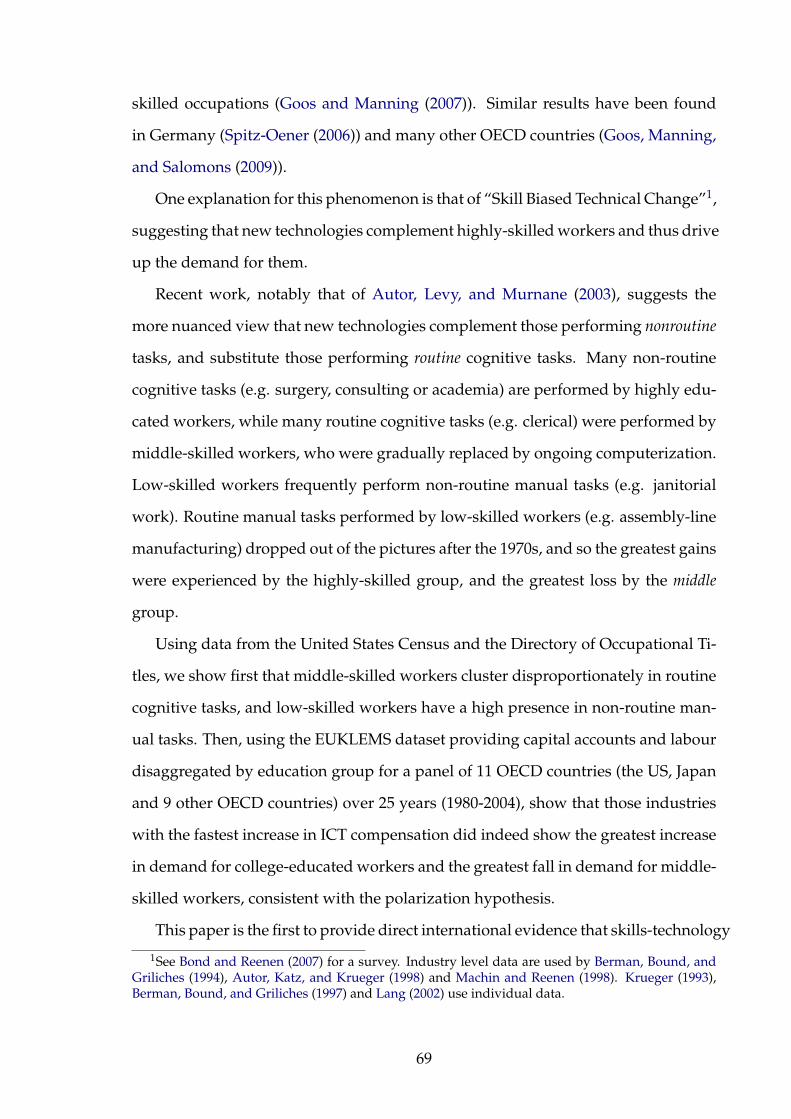
skilled occupations (Goos and Manning (2007)). Similar results have been found

in Germany (Spitz-Oener (2006)) and many other OECD countries (Goos, Manning,

and Salomons (2009)).

One explanation for this phenomenon is that of “Skill Biased Technical Change”1,

suggesting that new technologies complement highly-skilled workers and thus drive

up the demand for them.

Recent work, notably that of Autor, Levy, and Murnane (2003), suggests the

more nuanced view that new technologies complement those performing nonroutine

tasks, and substitute those performing routine cognitive tasks. Many non-routine

cognitive tasks (e.g. surgery, consulting or academia) are performed by highly edu-

cated workers, while many routine cognitive tasks (e.g. clerical) were performed by

middle-skilled workers, who were gradually replaced by ongoing computerization.

Low-skilled workers frequently perform non-routine manual tasks (e.g. janitorial

work). Routine manual tasks performed by low-skilled workers (e.g. assembly-line

manufacturing) dropped out of the pictures after the 1970s, and so the greatest gains

were experienced by the highly-skilled group, and the greatest loss by the middle

group.

Using data from the United States Census and the Directory of Occupational Ti-

tles, we show first that middle-skilled workers cluster disproportionately in routine

cognitive tasks, and low-skilled workers have a high presence in non-routine man-

ual tasks. Then, using the EUKLEMS dataset providing capital accounts and labour

disaggregated by education group for a panel of 11 OECD countries (the US, Japan

and 9 other OECD countries) over 25 years (1980-2004), show that those industries

with the fastest increase in ICT compensation did indeed show the greatest increase

in demand for college-educated workers and the greatest fall in demand for middle-

skilled workers, consistent with the polarization hypothesis.

This paper is the first to provide direct international evidence that skills-technology

1See Bond and Reenen (2007) for a survey. Industry level data are used by Berman, Bound, andGriliches (1994), Autor, Katz, and Krueger (1998) and Machin and Reenen (1998). Krueger (1993),Berman, Bound, and Griliches (1997) and Lang (2002) use individual data.

69

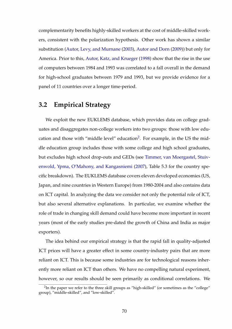
complementarity benefits highly-skilled workers at the cost of middle-skilled work-

ers, consistent with the polarization hypothesis. Other work has shown a similar

substitution (Autor, Levy, and Murnane (2003), Autor and Dorn (2009)) but only for

America. Prior to this, Autor, Katz, and Krueger (1998) show that the rise in the use

of computers between 1984 and 1993 was correlated to a fall overall in the demand

for high-school graduates between 1979 and 1993, but we provide evidence for a

panel of 11 countries over a longer time-period.

3.2 Empirical Strategy

We exploit the new EUKLEMS database, which provides data on college grad-

uates and disaggregates non-college workers into two groups: those with low edu-

cation and those with “middle level” education2. For example, in the US the mid-

dle education group includes those with some college and high school graduates,

but excludes high school drop-outs and GEDs (see Timmer, van Moergastel, Stuiv-

enwold, Ypma, O’Mahony, and Kangasniemi (2007), Table 5.3 for the country spe-

cific breakdown). The EUKLEMS database covers eleven developed economies (US,

Japan, and nine countries in Western Europe) from 1980-2004 and also contains data

on ICT capital. In analyzing the data we consider not only the potential role of ICT,

but also several alternative explanations. In particular, we examine whether the

role of trade in changing skill demand could have become more important in recent

years (most of the early studies pre-dated the growth of China and India as major

exporters).

The idea behind our empirical strategy is that the rapid fall in quality-adjusted

ICT prices will have a greater effect in some country-industry pairs that are more

reliant on ICT. This is because some industries are for technological reasons inher-

ently more reliant on ICT than others. We have no compelling natural experiment,

however, so our results should be seen primarily as conditional correlations. We

2In the paper we refer to the three skill groups as ”high-skilled” (or sometimes as the ”college”group), ”middle-skilled”, and ”low-skilled”.

70

do, however, implement some instrumental variable strategies using the industry-

specific initial levels of US ICT intensity and/or routine tasks as an instrument for

subsequent ICT increases in other countries. These support the OLS results. We con-

clude that technical change has raised relative demand for college educated workers

and, consistent with the ICT-based polarization hypothesis, this increase has come

mainly from reducing the relative demand for middle-skilled workers rather than

low-skilled workers.

Our approach of using industry and education is complementary to the alter-

native approach of using occupations and their associated tasks. Goos, Manning,

and Salomons (2011), for example, use wage and employment changes in occupa-

tions based on task content, for example, to show that “routine” occupations are in

decline and that these are in the middle of the wage distribution. In order to exam-

ine ICT-based theories of polarization, however, we believe it is important to have

direct measures of ICT capital. Such data is not generally available for individu-

als consistently across countries and years, which is why using the EUKLEMS data

is so valuable. As noted above, however, we do use the occupational information

to construct instrumental variables for the growth of ICT at the industry level over

time.

The paper is laid out as follows. Section II describes the empirical model, Section

III the data and Section IV the empirical results. Section V offers some concluding

comments.

3.3 Empirical Model

Consider the short-run variable cost function, CV(.):

CV(WH, WM, WL; C, K, Q) (3.1)

where W indicates hourly wages and superscripts denote education/skill group

S (H = highly educated workers, M = middle educated workers and L = low ed-

71

ucated workers), K = non-ICT capital services, C = ICT capital services and Q =

value added. If we assume that the capital stocks are quasi-fixed, factor prices are

exogenous and that the cost function can be approximated by a second order flexi-

ble functional form such as the translog, then cost minimization (using Shephard’s

Lemma) implies the following three skill share equations:

SHAREH = φHH ln(WH/WL)

+φMH ln(WM/WL)

+αCH ln(C/Q)

+αKH ln(K/Q)

+αQH ln Q

SHAREM = φHM ln(WH/WL)

+φMM ln(WM/WL)

+αCM ln(C/Q)

+αKM ln(K/Q)

+αQM ln Q

SHAREL = φHL ln(WH/WL)

+φML ln(WM/WL)

+αCL ln(C/Q)

+αKL ln(K/Q)

+αQM ln Q,

where SHARES= WS NS

WH NH+WS NM+WL NL is the wage bill share of skill group S =

72

{H, M, L} and NS is the number of hours worked by skill group S. Our hypoth-

esis of the ICT-based polarization theory is that αCH > 0 and αCM < 0 (with the sign

of αCL being ambiguous)3.

Our empirical specifications are based on these equations. We assume that labor

markets are national in scope and include country by time effects (φjt) to capture

the relative wage terms. We also check our results are robust to including industry-

specific relative wages directly on the right hand side of the share regressions. We

allow for unobserved heterogeneity between industry by country pairs (ηij) and in-

clude fixed effects to account for these, giving the following three equations:

SHARES = φjt + ηij + αCS ln(C/Q)ijt + αKS ln(K/Q)ijt + αQS ln Qijt, (3.2)

where i = industry, j =country and t = year. We estimate in long (25 year) dif-

ferences, ∆, to look at the historical trends and smooth out measurement error. We

substitute levels rather than logarithms (i.e. ∆(C/Q) instead of ∆ ln(C/Q)) because

of the very large changes in ICT intensity over this time period. Some industry by

country pairs had close to zero IT intensity in 1980 so their change is astronomical

in logarithmic terms4. Consequently our three key estimating equations are:

∆SHARESijt = cS

j + βS1∆(C/Q)ijt + βS

2∆(K/Q)ijt + βS3∆ ln Qijt + uS

ijt. (3.3)

In the robustness tests we also consider augmenting equation (3.3) in various

ways. Since ICT is only one aspect of technical change we also consider using Re-

search and Development (R&D) expenditures. This is a more indirect measure of

task-based technical change, but it has been used in the prior literature, so it could

be an important omitted variable. Additionally, we consider trade variables (such

3The exact correspondence between the coefficients on the capital inputs and the Hicks-Allenelasticity of complementarity is more complex (see Brown and Christensen (1981)).

4The range of ∆ ln(C/Q) lies between -1 and 23.5. We report robustness checks using ∆(C/Q)C/Q as

an approximation for ∆ ln(C/Q).

73

as imports plus exports over value added) to test whether industries that were ex-

posed to more trade upgraded the skills of their workforce at a more rapid rate than

those who did not. This is a pragmatic empirical approach to examining trade ef-

fects. Under a strict Heckscher-Ohlin approach trade is a general equilibrium effect

increasing wage inequality throughout the economy so looking at the variation by

industry would be uninformative. However, since trade costs have declined more

rapidly in some sectors than others (e.g. due to trade liberalization) we would ex-

pect the actual flows of trade to proxy this change and there to be a larger effect on

workers in these sectors than in others who were less affected (Krugman (2008) also

makes this argument).

3.4 Data

3.4.1 Data Construction

The main source of data for this paper is the EUKLEMS dataset, which contains

data on value added, labor, capital, skills and ICT for various industries in many

developed countries (see Timmer, van Moergastel, Stuivenwold, Ypma, O’Mahony,

and Kangasniemi (2007)). The EUKLEMS data are constructed using data from each

country’s National Statistical Office (e.g. the US Census Bureau) and harmonized

with each country’s national accounts. EUKLEMS contains some data on most

OECD countries. But since we require data on skill composition, ICT and non-

ICT capital and value added between 1980 and 2004, our sample of countries is

restricted to eleven: Austria, Denmark, Finland, France, Germany, Italy, Japan, the

Netherlands, Spain, the UK and the USA5.

Another choice we had to make regards the set of industries we analyze. Since

our baseline year (1980) was close to the peak of the oil boom, we have dropped

energy-related sectors - mining and quarrying, coke manufactures and the supply of

5In order to increase the number of countries we would need to considerably shorten the periodwe analyze. For example, limiting our analysis to 1992-2004 (12 years instead of 25) only adds Bel-gium. To further add Czech Republic, Slovenia and Sweden we would need to restrict the sample to1995-2004. In order to preserve the longer time series we focused on the 11 core OECD countries.

74

natural gas - from the sample (we report results that are very robust to the inclusion

of these sectors). The remaining sample includes 27 industries in each country (see

Table G.10). Wage data by skill category are only reported separately by industry

in some countries. We therefore aggregate industries to the lowest possible level of

aggregation for which all the variables we use could be constructed with the precise

level of disaggregation varied by country (see Table G.11)6. Our final sample has

208 observations on country-industry cells for 1980 and 2004. We also have data for

intervening years, which we use in some of the robustness checks.

For each country-industry-year cell in our dataset we construct a number of vari-

ables. Our main outcome is the wage bill share of workers of different educational

groups, which is a standard indicator for skill demand. In 9 of the 11 countries, the

high-skilled group indicates whether an employee has attained a college degree7. A

novel feature of our analysis is that we also consider the wage bill of middle-skilled

workers. The precise composition of this group varies across countries, since educa-

tional systems differ considerably. But typically, this group consists of high school

graduates, people with some college education, and people with non-academic pro-

fessional degrees.

Our main measure for use of new technology is Information and Communication

Technology (ICT) capital divided by value added. Similarly, we also use the mea-

sure of non-ICT capital divided by value added. EUKLEMS builds these variables

using the perpetual inventory method from the underlying investment flow data

for several types of capital. For the tradable industries (Agriculture and Manufac-

turing) we construct measures of trade flows using UN COMTRADE data8. Details

are contained in H.2.

Finally, we construct measures of skill and task content by occupation. We begin

6Results are robust to throwing away information and harmonizing all countries at the same levelof industry aggregation.

7In two countries the classification of high-skilled workers is different: in Denmark it includespeople in “long cycle” higher education and in Finland it includes people with tertiary education orhigher.

8Using a crosswalk (available from the authors upon request) we calculate the value of total trade,imports and exports with the rest of the world and separately with OECD and non-OECD countries.We identify all 30 countries that were OECD members in 2007 as part of the OECD.

75

with US Census micro data for 1980 from IPUMS, which identify each person’s ed-

ucation (which we aggregate to three skill levels using the EUKLEMS concordance

for the US) and occupation. We then use the “80-90” occupation classification from

Autor, Levy, and Murnane (2003) to add information on the task measures they con-

struct. These include routine cognitive tasks (measured using Set limits, Tolerances,

or Standards); routine manual tasks (measured using Finger Dexterity); non-routine

cognitive tasks measured using both (i) Quantitative reasoning requirements and

(ii) Direction, Control, and Planning and non-routine manual tasks (measured us-

ing Eye-Hand-Foot coordination). We standardize each of these five task measures

by subtracting the mean task score across occupations, weighted by person weights,

and dividing the result by the standard deviation of the measure across occupations.

3.4.2 Descriptive statistics

3.4.2.1 The Routineness of Occupations by Skill Level

We begin the description of the data by examining the relationship between ed-

ucation and tasks. Table G.2 reports the top 10 occupations for each of the three

education categories using US data for 1980. This table shows that the occupations

with the largest shares of highly-educated workers (such as physicians, lawyers and

teachers) and those with the highest shares of low-educated workers (such as clean-

ers and farm workers) have low scores on routine cognitive tasks. These groups

also have typically low scores on routine manual tasks. By contrast, occupations

with high shares of middle-educated workers (mostly clerical occupations and bank

tellers) typically score highly on both routine cognitive and routine manual tasks.

Therefore, if the only contribution of ICT was to automate (and replace) routine

tasks, it should benefit both high-skilled and low-skilled workers at the expense of

middle-skilled workers.

However, as argued by Autor, Levy, and Murnane (2003) information technol-

ogy should also complement non-routine tasks, especially cognitive ones. Here the

picture is more nuanced: high-skilled occupations typically score highly on non-

76

routine cognitive tasks, though not on non-routine manual tasks. Middle-skilled

occupations tend to score around average in non-routine tasks, while low-skilled

workers score low on non-routine cognitive tasks but above average on non-routine

manual tasks. Therefore, to the extent that information technology both replaces

routine tasks and complements non-routine tasks, the overall picture suggests that

ICT should increase the relative demand for high-skilled workers at the expense of

middle-skilled workers, with no clear effect on low-skilled workers.

We further explore the relationship between education groups and tasks in Table

G.1, which reports the average tasks content by skill group, again using 1980 US

data. On average, high-skilled occupations rank lowest in terms of routine tasks

and non-routine manual tasks, but highest in terms of non-routine cognitive tasks,

so the Autor, Levy, and Murnane (2003) model suggests that they benefit from ICT

improvements. Middle-skilled occupations score above-average on routine tasks

and a little below average on non-routine tasks, so ICT should probably reduce the

relative demand for their services. Lastly, the picture for low-skilled workers is once

again mixed, for both routine and non-routine tasks, so the theory gives no clear

prediction on how ICT improvements should affect the demand for their services.

Having discussed the relationship between skills and tasks, we now move on to

describe the changes in skill demand using the EUKLEMS data.

3.4.2.2 Cross Country Trends

Panel A of Table G.3 shows summary statistics for the levels of the key vari-

ables in 1980 across each country and Panel B presents the same for the changes

through 2004. The levels have to be interpreted with care as exact comparison of

qualifications between countries is difficult, which is why wage bill shares are use-

ful summary measures as each qualification is weighted by its price (the wage)9.

The ranking of countries looks sensible with the US having the highest share of

high-skilled (29 percent), followed by Finland (27 percent). All countries have ex-

9Estimating in differences also reduces the suspected bias from international differences as thedefinitions are stable within country over time.

77

perienced significant skill upgrading as indicated by the growth in the high-skilled

wage bill share in column (1) of Panel B, on average the share increased form 14.3

percent in 1980 to 24.3 in 2004.

The UK had the fastest absolute increase in the high-skilled wage bill share (16.5

percentage points) and is also the country with the largest increase in ICT intensity.

The US had the second largest growth of ICT and the third largest increase in the

high-skilled wage bill share (13.9 percentage points), but all countries have experi-

enced rapid increases in ICT intensity, which doubled its 1980 share of value added.

Figures F.1 to F.3 show the correlation between the growth of the wage bill share of

each of the three education groups and ICT intensity. There appears to be a posi-

tive relationship for the highly educated (Figure F.1), a negative relationship for the

middle educated (Figure F.2) and no relationship for the least educated (Figure F.3).

Although this is supportive of our model’s predictions, there are many other influ-

ences at the country-level so our econometric results below will focus on the within

country, across industry variation.

Returning to Table G.2, note that the change of the middle education share in

column (2) is more uneven. Although the mean growth is positive, it is relatively

small compared to the highly educated (8.7 percentage points on a base of 51.1 per-

cent), with several countries experiencing no growth or a decrease (the US and the

Netherlands).

Moreover, as Figures F.4 to F.5 shows, although the wage bill share of the middle

group rose more rapidly (in percentage point terms) between 1980 and 1986, it sub-

sequently decelerated. Indeed, in the last six year sub-period, 1998-2004, the wage

bill share of middle-skilled workers actually fell. At the same time, the wage bill

share of low-skilled workers continued to decline throughout the period 1980-2004,

but at an increasingly slower rate. Figure F.5 shows the US, the technology leader

that is often a future indicator for other nations. From 1998-2004 the wage bill share

of the middle educated declined more rapidly than that of the low-educated work-

ers. Figure F.5 is in line with the finding that while college educated US workers

78

continued to gain relative to high-school graduates, high-school graduates gained

relatively to college dropouts in the 1980s but not in the 1990s (see Autor, Katz, and

Kearney (2008)).

3.4.2.3 Cross Industry Trends

Tables G.4 and G.5 break down the data by industry. In levels (Table G.4) the

highly educated were disproportionately clustered into services both in the public

sector (especially education) and private sector (e.g. real estate and business ser-

vices). The industries that upgraded skills rapidly (Table G.5) were also mainly ser-

vices (e.g. finance, telecoms and business services), but also in manufacturing (e.g.

chemicals and electrical equipment). At the other end of the skill distribution, the

textile industry, which initially had the lowest wage bill share of skilled workers,

upgraded somewhat more than other low-skill industries (transport and storage,

construction, hotels and restaurants, and agriculture). This raises the issue of mean

reversion, so we are careful to later show robustness tests to conditioning on the

initial levels of the skill shares in our regressions. In fact, the ranking of industries

in terms of skill intensity in 1980 and their skill upgrading over the next 25 years

was quite similar across countries. This is striking, because the countries we ana-

lyze had different labor market institutions and different institutional experiences

over the period we analyze. This suggests something fundamental is at play that

cuts across different sets of institutions.

ICT grew dramatically from 1980-2004, accounting for more than 42 percent of

the average increase in capital services (see columns (8) and (9) of Table G.5). The

increased ICT diffusion was also quite uneven: financial intermediation and tele-

coms experienced rapid increases in ICT intensity, while in other industries, such as

agriculture, there was almost no increase.

Figures F.6, F.7, F.8, F.9, and F.10 and F.11 plot changes by industry in the wage

bill shares of high, medium, and low-skilled workers, respectively, against changes

in ICT intensity. The top panel (A) of each figure includes all industries with fitted

79

regression lines (solid line for all industry and dashed line for non-traded sectors

only). The bottom panel (B) restricts attention to the traded sectors. Figure F.6 shows

that the industries with the fastest ICT upgrading had the largest increase in the

high-skilled wage bill share. One might be worried that two service sectors, “Post &

Telecommunications” and “Financial Intermediation”, are driving this result, which

is one reason Figure F.7 drops all the non-traded sectors. In fact, the relationship

between high-skilled wage bill growth and ICT growth is actually stronger in these

“well measured” sectors.

Figures F.8 and F.9 repeat this analysis for the middle educated groups. We ob-

serve the exact opposite relationship to Figures F.6 and F.7: the industries with the

faster ICT growth had the largest fall in the middle-skilled share whether we look

at the whole economy (Figure F.8) or just the traded sectors (Figure F.9). Finally,

Figures F.10 and F.11 show that there is essentially no relationship (Figure F.10) or a

mildly positive one (Figure F.11) between the change of the share of the least edu-

cated and ICT growth.

These figures are highly suggestive of empirical support for the hypothesis that

ICT polarizes the skill structure: increasing demand at the top, reducing demand in

the middle and having little effect at the bottom. To examine this link more rigor-

ously, we now turn to the econometric analysis.

3.5 Econometric Results

3.5.1 Basic Results

Our first set of results for the skill share regressions are reported in Table G.6.

The dependent variables are changes from 1980-2004 in the wage bill share of the

high-skilled in Panel A, the middle-skilled in Panel B and the low-skilled in Panel

C. The first four columns look across the entire economy and the last four columns

condition on the sub-sample of “tradable” sectors where we have information on

imports and exports.

80

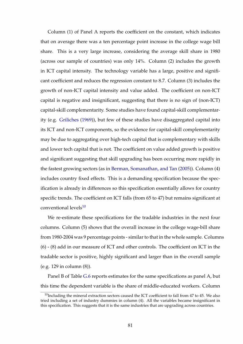
Column (1) of Panel A reports the coefficient on the constant, which indicates

that on average there was a ten percentage point increase in the college wage bill

share. This is a very large increase, considering the average skill share in 1980

(across our sample of countries) was only 14%. Column (2) includes the growth

in ICT capital intensity. The technology variable has a large, positive and signifi-

cant coefficient and reduces the regression constant to 8.7. Column (3) includes the

growth of non-ICT capital intensity and value added. The coefficient on non-ICT

capital is negative and insignificant, suggesting that there is no sign of (non-ICT)

capital-skill complementarity. Some studies have found capital-skill complementar-

ity (e.g. Griliches (1969)), but few of these studies have disaggregated capital into

its ICT and non-ICT components, so the evidence for capital-skill complementarity

may be due to aggregating over high-tech capital that is complementary with skills

and lower tech capital that is not. The coefficient on value added growth is positive

and significant suggesting that skill upgrading has been occurring more rapidly in

the fastest growing sectors (as in Berman, Somanathan, and Tan (2005)). Column (4)

includes country fixed effects. This is a demanding specification because the spec-

ification is already in differences so this specification essentially allows for country

specific trends. The coefficient on ICT falls (from 65 to 47) but remains significant at

conventional levels10

We re-estimate these specifications for the tradable industries in the next four

columns. Column (5) shows that the overall increase in the college wage-bill share

from 1980-2004 was 9 percentage points - similar to that in the whole sample. Columns

(6) - (8) add in our measure of ICT and other controls. The coefficient on ICT in the

tradable sector is positive, highly significant and larger than in the overall sample

(e.g. 129 in column (8)).

Panel B of Table G.6 reports estimates for the same specifications as panel A, but

this time the dependent variable is the share of middle-educated workers. Column

10Including the mineral extraction sectors caused the ICT coefficient to fall from 47 to 45. We alsotried including a set of industry dummies in column (4). All the variables became insignificant inthis specification. This suggests that it is the same industries that are upgrading across countries.

81

(1) shows that the wage bill share of middle-skilled workers grew by 8.7 percent-

age points over this time period. But as the rest of the panel shows, the association

between the change in middle-skilled workers and ICT is strongly negative. In col-

umn (4), for example, a one percentage point increase in ICT intensity is associated

with a 0.8 percentage point fall in the proportion of middle-skilled workers. The

magnitude of the coefficients for the sample that includes all industries is quite sim-

ilar to those for college educated workers. Panel C shows that technology measures

appear to be insignificant for the least educated workers, illustrating the point that

the main role of ICT appears to be in changing demand between the high-skilled

and middle-skilled groups11. Since the adding up requirement means that the coef-

ficients for the least skilled group can be deduced from the other two skill groups

we save space by omitting Panel C in the rest of the Tables.

Overall, Table G.6 shows a pattern of results consistent with ICT based polariza-

tion. Industries where ICT grew most strongly where those with the largest shifts

towards the most skilled and the largest shifts away from the middle skilled, with

the least skilled largely unaffected.

3.5.2 Robustness and Extensions

3.5.2.1 Initial conditions

Table G.7 examines some robustness checks using the results in our preferred

specification of column (4) of Table G.6 (reproduced in the first column). Since there

may be mean reversion we include the level of initial share of skills in 1980 in col-

umn (2). This does not qualitatively alter the results, although coefficient on ICT for

the middle-skilled does fall somewhat 12.11The difference in the importance of ICT for the middle and lowest skill groups implies that high

school graduates are not perfect substitutes for college graduates as Card (2009) argues in the UScontext. The majority of our data is from outside the US, however, where there are relatively fewerhigh school graduates.

12As we explain above our specifications assume that markets are national in scope, so that coun-try fixed effects capture changes in relative wages. To further test this assumption we re-estimatedcolumns (1) and (2) in Table 6 with additional controls for the change in the difference in industryspecific relative ln(wages) between the high-skilled and middle-skilled and between the high-skilledand low-skilled. The resulting coefficients (standard errors) on our measure of ICT are 41.43 (15.24)and 35.98 (14.82) for high-skilled workers, and -54.38 (20.96) and -33.35 (13.87) for middle-skilled

82

3.5.2.2 Timing of changes in skills and ICT

One limitation of the specifications that we discussed so far is that the changes

on the right-hand side and left hand-side are both concurrent. To mitigate potential

concerns about reverse causation, we re-estimate the baseline specification of col-

umn (1) Table G.7, where the right hand side variables are measured for the first half

of the period we consider (1980-1992) and the left hand side variable is measured for

the second half of the period (1992-2004). The estimated coefficients (and standard

errors) on changes in our measure of ICT are 52.62 (23.53) for high-skilled workers

and -52.52 (28.97) for middle-skilled workers. These results are almost unchanged

(51.31 (22.65) and -58.22 (22.99) respectively) when we instead use the equivalent of

the specification in column (2) of Table 6.

3.5.2.3 Heterogeneity in the coefficients across countries

Wage inequality rose less in Continental Europe than elsewhere, so it is inter-

esting to explore whether technological change induced polarization even there.

Columns (3) and (4) of Table G.7 restrict the sample to the 8 Continental Euro-

pean countries (Austria, Denmark, Finland, France, Germany, Italy, Netherlands

and Spain), and the results are similar to those in the full sample of countries. For

example, column (5) shows that the correlation between ICT and polarization is

larger for the US than for the full sample, though column (5) shows that the esti-

mates become imprecise when we control for baseline levels of skill composition.

The sample size for most individual countries is rather small, but if we re-estimate

the specification of Table G.7 column (2) separately country by country we obtain

negative coefficients on ICT for all 11 countries for medium skill shares and positive

coefficients for 10 countries for the high skill shares (Japan is the single exception)13.

The results are also robust to dropping any single country14.

workers.13The mean of the 11 country-specific coefficients on ICT is very similar to the pooled results (-112

for the middle-skilled share and 71 for the high-skilled share).14For example, we had concerns about the quality of the education data in Italy so we dropped

Italy from the sample. In the specification of column (4) of Table G.6, the coefficient (standard error)on ICT capital was 55.2(1.04) for the high education group and -68.54(22.82) for the middle educated.

83

3.5.2.4 Instrumental variables

One concern is that measurement error in the right hand side variables, espe-

cially our measure of ICT, causes attenuation bias15. To mitigate this concern, we

use the industry-level measures of ICT in the US in 1980 as an instrument for ICT

upgrading over the whole sample. The intuition behind this instrument is that the

dramatic global fall in quality-adjusted ICT prices since 1980 (e.g. Jorgenson, Ho,

and Stiroh (2008)) disproportionately affects industries that (for exogenous techno-

logical reasons) have a greater potential for using ICT inputs. An indicator of this

potential is the initial ICT intensity in the technological leader, the US. As column

(7) of Table G.7 shows, this instrument has a first-stage F-statistic of 10.5, and the

sign of the first stage regressions (not reported) is as we would expect, namely in-

dustries that were more ICT-intensive in 1980 upgraded their use of ICT more than

others. In the 2SLS estimates of column (7) the coefficient on ICT is roughly twice

as large as the OLS coefficients for the college educated group (and significant at

the 5 percent level), and a little bigger for the middle-skilled group. Column (8) re-

port estimates the same specification but this time excluding the US itself, and the

results are very similar. While we acknowledge that estimates using this instrument

do not necessarily uncover the causal effect of ICT, it is reassuring that these 2SLS

estimates are somewhat larger than the OLS estimates, as we would expect given

the likely measurement error.

As a further check, we use the proportion of routine tasks in the industry (in the

US in the base year) as an instrument for future ICT growth as these industries were

most likely to be affected by falling ICT prices (see Autor and Dorn, 2009). The re-

sults of using this instrument are shown in columns (9) and (10). Although the first

stages are weaker with this instrument16, and the 2SLS estimates are not very pre-

15Estimates of the ICT coefficient for the two 12-year sub-periods of our data are typically abouthalf of the absolute magnitude of those for the full period. In general, our estimates for shorter timeperiods are smaller and less precise, consistent with the importance of measurement error in the ICTdata. For example, in the specification of column (4) of Panel A in Table G.6, the coefficient (standarderror) on ICT was 18.30 (10.30) in a pooled 12 year regression. We could not reject the hypothesis thatthe ICT coefficient was stable over time (p-value=0.35).

16The signs of the instruments in the first stage are correct. The F-test is 6.5 in column (9) compared

84

cise, these columns again suggest that we may be under-estimating the importance

of ICT by just using OLS.

3.5.2.5 Disaggregating the wage bill into wages and hours

The wage bill share of each skill group reflects its hourly wage and hours worked,

and those of the other skill groups. We estimated specifications that are identical to

those in Table G.6, except that they disaggregate the dependent variable into the

growth of relative skill prices and quantities. In the first two columns of Table G.8

we reproduce the baseline specifications using the log relative wage bill (which can

be exactly decomposed) as the dependent variable17. Columns (1) - (4) confirm what

we have already seem using a slightly different functional form: ICT growth is asso-

ciated with a significant increase in the demand for high-skilled workers relative to

middle-skilled workers (first two columns) and with a significant (but smaller) in-

crease for low-skilled workers relative to middle-skilled workers (third and fourth

columns).

For the high vs. middle-skill group, ICT growth is significantly associated with

increases in relative wages and relative hours (columns (5), (6), (9) and (10)). In

comparing the middle vs. low groups, the coefficients are also all correctly signed,

but not significant at conventional levels. Overall this suggests that our results are

robust to functional form and the shifting pattern of demand operates both through

wages and hours worked18.

3.5.3 Trade, R&D and skill upgrading

Having found that technology upgrading is associated with substitution of college-

educated workers for middle-educated workers, we now examine whether changes

to 10.5 in column (7).17Another functional form check was using the growth rate of ICT intensity. For the specification

in column (3) of Panel A in Table G.6 we replaced ∆(C/Q) with ∆(C/Q)C/Q . The coefficient (standard

error) on ICT growth was 2.586 (1.020). The marginal effect of a one standard deviation increase(0.581) is 1.50 (=0.581*2.586), almost identical to 1.55 (=0.024*64.6) in Table G.6.

18In examining these results across countries there was some evidence that the adjustment in wageswas stronger in the US and the adjustment in hours was stronger in Continental Europe. This isconsistent with the idea of great wage flexibility in the US than in Europe.

85

in trade exhibit similar patterns. The first three columns of Table G.9 suggest that

more trade openness (measured as the ratio of imports plus exports to value added)

is associated with increases in the wage bill share of college educated workers and

declines in the share for middle-skilled workers. However, the when we control

for initial R&D intensity the association between trade and skill upgrading becomes

smaller and insignificant. Column (4) repeats the specification of column (3) for the

sub-sample where we have R&D data and shows that the trade coefficient is ro-

bust. Column (5) includes R&D intensity in a simple specification and shows that

the coefficient on trade falls (e.g. from 0.50 to 0.24 in Panel A) and is insignificant,

whereas the coefficient on R&D is positive and significant. In column (6) we include

the changes in the ICT and non-ICT capital stocks and the coefficient on trade is

now very small. Column (7) drops the insignificant trade variable and shows that

ICT and R&D and individually (and jointly) significant.

We also used the Feenstra and Hansen (1999) method of constructing an off-

shoring variable and included it instead of (and alongside) trade in final goods. The

offshoring variable has more explanatory power than final goods trade19. Column

(8) includes offshoring (“Imported Intermediate Inputs”) into the full sample as it

can be defined for all industries. The results suggest a significant positive correla-

tion between offshoring for high skilled workers and a negative but insignificant

correlation between ICT and demand for middle skilled workers. Column (9) pro-

duces a similar result on the sample of tradable sectors and column (10) includes

ICT and R&D. As with the trade measure in final goods, the offshoring coefficient is

driven to zero in the final column for the highly educated and remains insignificant

for the middle educated. The ICT effects are robust to the inclusion of the offshoring

measures.

These findings are broadly consistent with most of the literature that finds that

technology variables have more explanatory power than trade in these kinds of skill

19For example, in the same specification of column (6) of Table G.9 we replaced the final goodstrade variable with the offshoring measure. In the high skilled equation the coefficient (standarderror) was 4.27 (2.82) and in the middle skilled equation the coefficient (standard error) was -11.6(9.87).

86

demand equations20. Of course, trade could be influencing skill demand through

affecting the incentives to innovate and adopt new technologies, which is why trade

ceases to be important after we condition on technology (e.g. Bloom, Draca, and

Reenen (2011), argue in favor of this trade-induced technical change hypothesis)21.

Furthermore, there could be many general equilibrium effects of trade that we have

not accounted for (these are controlled for by the country time effects).

3.5.4 Magnitudes

We perform some “back of the envelope” calculations in Table G.13 to gauge the

magnitude of the effect of technology on the demand for highly skilled workers.

Column (1) estimates that ICT accounts for 13.2 percent of the increase in the col-

lege share in the whole sample without controls and column (2) reduces this to 8.5

percent with controls. Many authors (e.g. Jorgenson, Ho, and Stiroh (2008)) have

argued that value added growth has been strongly affected by ICT growth, espe-

cially in the later period, so column (2) probably underestimates the effect of ICT.

Column (3) reports equivalent calculations for the tradable sectors. Here, ICT ac-

counts for 16.5 percent of the change and R&D a further 16.1 percent, suggesting

that observable technology measures by account for almost a third of the increase

in demand for highly skilled workers. If we include controls in column (4) this falls

to 23.1 percent. Finally, columns (5) and (6) report results for the IV specification for

the whole sample, showing an ICT contribution of ICT of between 22.1 percent and

27.7 percent22.

20These are simple industry-level correlations and not general equilibrium calculations, so we maybe missing out the role of trade through other routes.

21We further test whether the association between trade and skill upgrading remains similar whenwe examine different components of trade separately. Table G.12 suggests that when we examine im-ports and exports separately, the picture is quite similar. Greater trade is associated with an increasein the college wage bill share until we control for initial R&D intensity, in which case the coefficienton trade falls and becomes insignificant. Results are similar when we analyze separately imports to(or exports from) OECD countries. For non-OECD countries the results are again the same, exceptfor exports to non-OECD countries, which remains positively associated with changes in the collegewage-bill share even after we add all the controls, including R&D. However, it should be noted thatthe change in exports to developing countries is on average very small.

22The IV specifications for tradeables show an even larger magnitude. For example in a specifica-tion with full controls, R&D and ICT combined account for over half of all the change in the collegewage bill share. The first stage for the IV is weak, however, with an F-statistic of 6, these cannot be

87

We also note that while ICT upgrading alone should have led to decreased de-

mand for middle-skilled workers. While we do not see such a decrease overall, Fig-

ure F.5 shows a slowdown in the growth of demand for middle skilled over time,

and a reversal (in other words negative growth) for middle-skilled workers from

1998-2004.

We have no general equilibrium model, so these are only “back of the envelope”

calculations to give an idea of magnitudes. Furthermore, measurement error prob-

ably means that we are probably underestimating the importance of the variables.

Nevertheless, it seems that our measures of technology are important in explaining

a significant proportion of the increase in demand for college educated workers at

the expense of the middle-skilled.

3.6 Conclusions

Recent investigations into the changing demand for skills in OECD countries

have found some evidence for “polarization” in the labour market in the sense that

workers in the middle of the wage and skills distribution appear to have fared more

poorly than those at the bottom and the top. One explanation that has been ad-

vanced for this is that ICT has complemented non-routine analytic tasks but substi-

tuted for routine tasks whilst not affecting non-routine manual tasks (like cleaning,

gardening, childcare, etc.). This implies that many middle-skilled groups like bank

clerks and paralegals performing routine tasks have suffered a fall in demand. To

test this we have estimated industry-level skill share equations distinguishing three

education groups and related this to ICT (and R&D) investments in eleven coun-

tries over 25 years using newly available data. Our findings are supportive of the

ICT-based polarization hypothesis as industries that experienced the fastest growth

in ICT also experienced the fastest growth in the demand for the most educated

workers and the fastest falls in demand for workers with intermediate levels of ed-

ucation. The magnitudes are nontrivial: technical change can account for up to a

relied on.

88

quarter of the growth of the college wage bill share in the economy as a whole (and

more in the tradable sectors).

Although our method is simple and transparent, there are many extensions that

need to be made. First, alternative instrumental variables for ICT would help iden-

tify the causal impact of ICT. Second, although we find no direct role for trade vari-

ables, there may be other ways in which globalization influences the labour market,

for example by causing firms to “defensively innovate” (Acemoglu (2003)). Third,

there are alternative explanations for the improved performance of the least skilled

group through for example, greater demand from richer skilled workers for the ser-

vices they provide as market production substitutes for household production (e.g.

childcare, eating out in restaurants, domestic work, etc.)23. These explanations may

complement the mechanism that we address here. Finally, we have not used richer

occupational data that would focus on the skill content of tasks due to the need

to have international comparability across countries. The work of Autor and Dorn

(2009) is an important contribution here.

23Ngai and Pissarides (2007), Mazzolari and Ragusa (2008)

89

Appendix A

Figures: Chapter 1

Figure A.1 Allocation of SC seats to a district

Figure A.2 Identification of District Cutoff

90

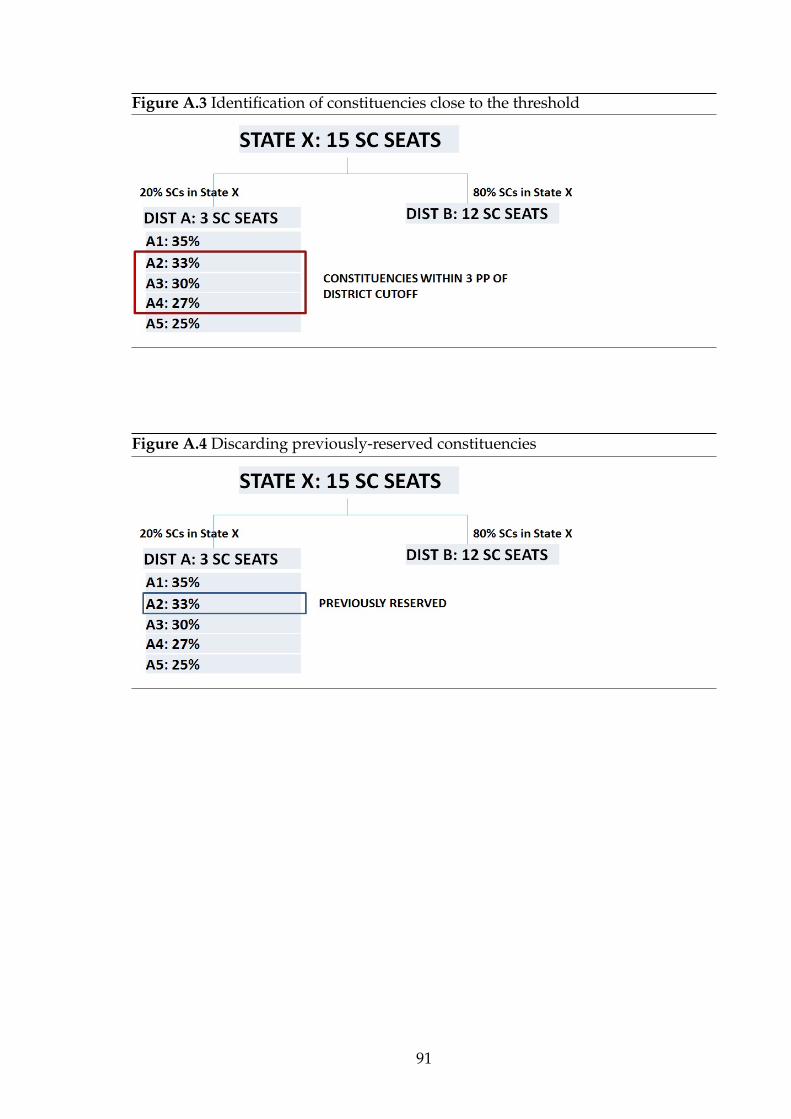
Figure A.3 Identification of constituencies close to the threshold

Figure A.4 Discarding previously-reserved constituencies

91

Figure A.5 Identification of Treatment and Control Groups

92

Appendix B

Tables: Chapter 1

Table B.1: Constituency Averages: Chhatisgarh, Karnataka, Madhya Pradesh andRajasthan 2001

Treated Untreated Difference

Observations 38 69

Total Population 32729 45679 -12950(12417) (10558) (16276)

Fraction of Scheduled Castes (SC) 0.21 0.20 0.01(0.01) (0.01) (0.01)

Fraction of Scheduled Tribes (ST) 0.11 0.09 0.02(0.02) (0.01) (0.02)

Fraction of Females 0.48 0.48 -0.001(0.002) (0.001) (0.003)

Fraction of Illiterates 0.53 0.53 -0.003(0.01) (0.01) (0.02)

Employed as a Fraction of Total Population 0.47 0.48 -0.01(0.01) (0.01) (0.01)

Notes: top row: Averages at constituency level. Standard error clustered at constituency level inparentheses. All data taken from the 2001 Census data for Chhatisgarh, Madhya Pradesh,

Karnataka and Rajasthan.

93

Table B.2: Constituency Electoral Characteristics


Observations 38 69

Panel A: Constituency Electoral Characteristics at Baseline: 2003 and 2004

Electors 168060 165826 2234(3475) (2740) (4419)

Female candidates 0.05 0.06 -0.01(0.01) (0.01) (0.02)

Candidates from Right-wing Parties 0.11 0.14 -0.03(0.01) (0.01) (0.01)

Candidates from Left/Centre-Left Parties 0.16 0.19 -0.03(0.01) (0.01) (0.01)

Candidates from Lower-Caste Parties 0.14 0.10 0.03(0.01) (0.01) (0.02)

Female candidates winning 0.03 0.03 0.00(0.03) (0.02) (0.03)

Candidates from Right-wing Parties winning 0.53 0.57 -0.04(0.08) (0.06) (0.10)

Candidates from Left/Centre-Left Parties winning 0.18 0.33 -0.15(0.06) (0.06) (0.09)

Candidates from Lower-Caste Parties winning 0.03 0.01 0.01(0.03) (0.01) (0.03)

Panel B: Constituency Electoral Characteristics in 2008

Electors 170311 172300 -1990(3682) (2510) (4447)

Female candidates 0.08 0.06 0.02(0.02) (0.01) (0.02)

Candidates from Right-wing Parties 0.09 0.11 -0.01(0.01) (0.004) (0.01)

Candidates from Left/Centre-Left Parties 0.11 0.14 -0.02(0.01) (0.01) (0.01)

Candidates from Lower-Caste Parties 0.13 0.13 -0.003(0.01) (0.01) (0.01)

Female candidates winning 0.18 0.14 0.04(0.06) (0.04) (0.08)

Candidates from Right-wing Parties winning 0.63 0.41 0.23(0.08) (0.06) (0.10)

Candidates from Left/Centre-Left Parties winning 0.26 0.46 -0.20(0.07) (0.06) (0.09)

Candidates from Lower-Caste Parties winning 0.03 0.01 0.01(0.03) (0.01) (0.03)

Notes: Standard error of mean in parentheses. All data taken from the 2003 and 2004 ElectionCommission of India State Legislative Assembly Results for Chhatisgarh, Madhya Pradesh,

Rajasthan and Karnataka.”Left” parties are: the Communist Party of India (and offshoots) and theIndian National Congress; ”Right” parties: the Bharatiya Janata Party (BJP); ”Lower-caste” parties:

the Bahujan Samaj Party (BSP).94

Table B.3: Averages of Dependent Variables

Pre Post Difference

TurnoutTreated 0.69 0.63 -0.05

(0.01) (0.01) (0.01)Untreated 0.70 0.70 0.00

(0.01 (0.01) (0.00)Difference -0.01 -0.07 -0.06

(0.01) (0.01) (0.01)Log (Candidates/Electors)

Treated 3.94 4.23 0.30(0.06) (0.07) (0.07)

Untreated 3.86 4.07 0.22(0.05) (0.05) (0.05)

Difference 0.08 0.16 0.08(0.07) (0.09) (0.08)

Margin of VictoryTreated 0.11 0.11 0.00

(0.01) (0.01) (0.02)Untreated 0.12 0.09 -0.03

(0.01) (0.01) (0.01)Difference 0.00 0.02 0.03

(0.02) (0.02) (0.02)Right-wing candidates winning

Treated 0.53 0.63 0.11(0.08) (0.08) (0.11)

Untreated 0.57 0.41 -0.16(0.06) (0.06) (0.08)

Difference -0.04 0.23 0.26(0.10) (0.10) (0.13)

Centre/Centre-Left candidates winningTreated 0.18 0.26 0.08

(0.06) (0.07) (0.10)Untreated 0.33 0.46 0.13

(0.06) (0.06) (0.08)Difference -0.15 -0.20 -0.05

(0.09) (0.09) (0.13)Lower-Caste party candidates winningTreated 0.03 0.03 0.00

(0.03) (0.03) (0.04)Untreated 0.01 0.01 0.00

(0.01) (0.01) (0.02)Difference 0.01 0.01 0.00

(0.03) (0.03) (0.04)Notes: Number of Treated Constituencies: 38. Number of Untreated Constituencies: 69. Standarderror of mean in parentheses. All data taken from the 2003, 2004 and 2008 Election Commission of

India State Legislative Assembly Results for Chhatisgarh, Madhya Pradesh, Rajasthan andKarnataka.”Right” parties: the Bharatiya Janata Party (BJP). Candidates/Electors multiplied

everywhere by 1000000.

95

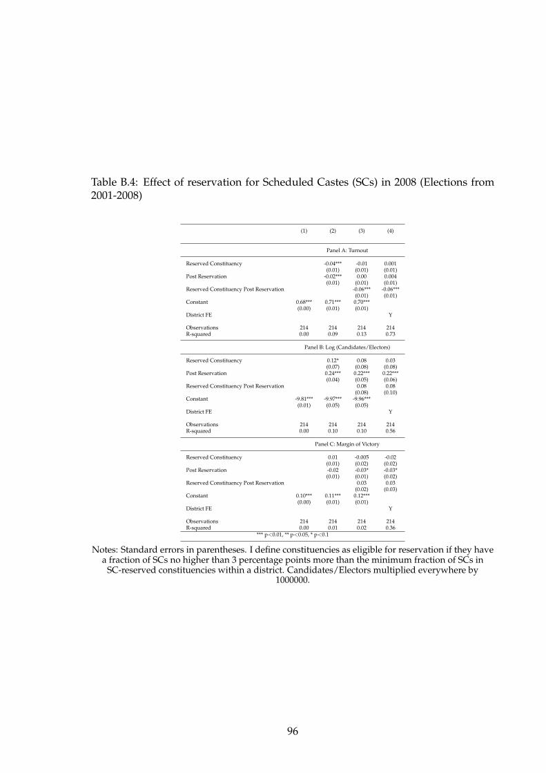
Table B.4: Effect of reservation for Scheduled Castes (SCs) in 2008 (Elections from2001-2008)

(1) (2) (3) (4)

Panel A: Turnout

Reserved Constituency -0.04*** -0.01 0.001(0.01) (0.01) (0.01)

Post Reservation -0.02*** 0.00 0.004(0.01) (0.01) (0.01)

Reserved Constituency Post Reservation -0.06*** -0.06***(0.01) (0.01)

Constant 0.68*** 0.71*** 0.70***(0.00) (0.01) (0.01)

District FE Y

Observations 214 214 214 214R-squared 0.00 0.09 0.13 0.73

Panel B: Log (Candidates/Electors)

Reserved Constituency 0.12* 0.08 0.03(0.07) (0.08) (0.08)

Post Reservation 0.24*** 0.22*** 0.22***(0.04) (0.05) (0.06)

Reserved Constituency Post Reservation 0.08 0.08(0.08) (0.10)

Constant -9.81*** -9.97*** -9.96***(0.01) (0.05) (0.05)

District FE Y


Panel C: Margin of Victory

Reserved Constituency 0.01 -0.005 -0.02(0.01) (0.02) (0.02)

Post Reservation -0.02 -0.03* -0.03*(0.01) (0.01) (0.02)

Reserved Constituency Post Reservation 0.03 0.03(0.02) (0.03)

Constant 0.10*** 0.11*** 0.12***(0.00) (0.01) (0.01)

District FE Y


*** p<0.01, ** p<0.05, * p<0.1

Notes: Standard errors in parentheses. I define constituencies as eligible for reservation if they havea fraction of SCs no higher than 3 percentage points more than the minimum fraction of SCs in

SC-reserved constituencies within a district. Candidates/Electors multiplied everywhere by1000000.

96

Table B.5: Effect of reservation for Scheduled Castes (SCs) in 2008 (Elections from2001-2008) on Incidence of Victory of Party Categories

(1) (2) (3) (4)

Panel A: Right-Wing

Reserved Constituency -0.04 0.08 -0.10(0.10) (0.11) (0.26)

Post Reservation -0.16* -0.16* -0.40*(0.08) (0.10) (0.21)

Reserved Constituency Post Reservation 0.26** 0.26* 0.67**(0.13) (0.15) (0.34)

Constant 0.52*** 0.57*** 0.16(0.04) (0.06) (0.15)

Specification OLS OLS OLS PROBITDistrict FE YObservations 214 214 214 99R-squared 0.00 0.03 0.34 0.02

Panel B: Centre/Centre-Left

Reserved Constituency -0.15* -0.21** -0.47*(0.09) (0.10) (0.28)

Post Reservation 0.13 0.13 0.34(0.08) (0.09) (0.21)

Reserved Constituency Post Reservation -0.05 -0.05 -0.07(0.13) (0.15) (0.40)

Constant 0.34*** 0.33*** -0.51***(0.03) (0.06) (0.16)


Panel C: Lower-Caste Parties

Reserved Constituency 0.01 -0.02 0.25(0.03) (0.03) (0.58)

Post Reservation -0.00 0.00 -0.00(0.02) (0.02) (0.56)

Reserved Constituency Post Reservation 0.00 -0.00 0.00(0.04) (0.05) (0.83)

Constant 0.02** 0.01 -2.18***(0.01) (0.01) (0.39)


*** p<0.01, ** p<0.05, * p<0.1

Notes: Standard errors in parentheses. I define constituencies as eligible for reservation if they havea fraction of SCs no higher than 3 percentage points more than the minimum fraction of SCs in

SC-reserved constituencies within a district.

97

Table B.6: Effect of dereservation for Scheduled Castes (SCs) in 2008 (Elections from2001-2008)

(1) (2) (3) (4) (5) (6)

Turnout Log(Candidates Margin of Victory/Electors)

Reserved Constituency 0.00 0.03 -0.02(0.01) (0.08) (0.02)

Post Reservation 0.00 0.01 0.22*** 0.18 -0.03* -0.06(0.01) (0.01) (0.06) (0.12) (0.02) (0.04)

Reserved Constituency -0.06*** 0.08 0.02Post Reservation (0.01) (0.10) (0.03)Dereserved Constituency 0.06*** -0.02 -0.02

(0.02) (0.21) (0.03)Dereserved Constituency 0.04** 0.43** 0.03Post Dereservation (0.02) (0.18) (0.05)Observations 214 99 214 99 214 99R-squared 0.73 0.87 0.56 0.68 0.3 0.38

Right-Wing Centre/Centre-Left Lower-CasteParties Parties Parties


Post Reservation -0.16* -0.24 0.13 0.29 0.00 0.00(0.1) (0.20) (0.09) (0.20) (0.02) (0.00)

Reserved Constituency 0.26* -0.05 -0.00Post Reservation (0.16) (0.15) (0.05)Dereserved Constituency -0.07 0.04 -0.04

(0.22) (0.22) (0.03)Dereserved Constituency 0.09 -0.22 0.07Post Dereservation (0.27) (0.27) (0.07)Observations 214 99 214 99 214 99R-squared 0.35 0.44 0.33 0.39 0.36 0.53

*** p<0.01, ** p<0.05, * p<0.1

Notes: Standard errors in parentheses. I define constituencies as eligible for reservation if they havea fraction of SCs no higher than 3 percentage points more than the minimum fraction of SCs inSC-reserved constituencies within a district. All regressions have district and year fixed effects.Standard errors are clustered by constituency. Candidates/Electors multiplied everywhere by

1000000.

98

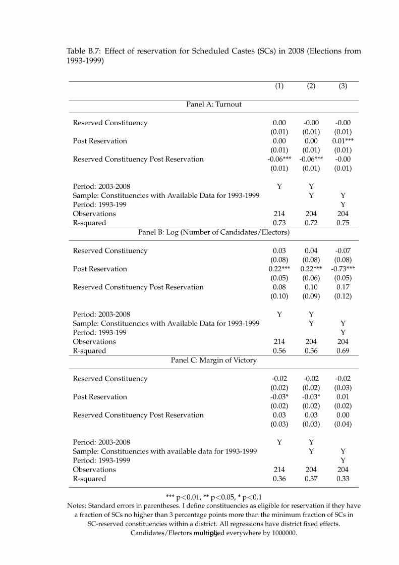
Table B.7: Effect of reservation for Scheduled Castes (SCs) in 2008 (Elections from1993-1999)

(1) (2) (3)

Panel A: Turnout


Post Reservation 0.00 0.00 0.01***(0.01) (0.01) (0.01)

Reserved Constituency Post Reservation -0.06*** -0.06*** -0.00(0.01) (0.01) (0.01)

Period: 2003-2008 Y YSample: Constituencies with Available Data for 1993-1999 Y YPeriod: 1993-199 YObservations 214 204 204R-squared 0.73 0.72 0.75

Panel B: Log (Number of Candidates/Electors)


Post Reservation 0.22*** 0.22*** -0.73***(0.05) (0.06) (0.05)

Reserved Constituency Post Reservation 0.08 0.10 0.17(0.10) (0.09) (0.12)


Panel C: Margin of Victory

Reserved Constituency -0.02 -0.02 -0.02(0.02) (0.02) (0.03)

Post Reservation -0.03* -0.03* 0.01(0.02) (0.02) (0.02)

Reserved Constituency Post Reservation 0.03 0.03 0.00(0.03) (0.03) (0.04)

Period: 2003-2008 Y YSample: Constituencies with available data for 1993-1999 Y YPeriod: 1993-1999 YObservations 214 204 204R-squared 0.36 0.37 0.33

*** p<0.01, ** p<0.05, * p<0.1Notes: Standard errors in parentheses. I define constituencies as eligible for reservation if they have

a fraction of SCs no higher than 3 percentage points more than the minimum fraction of SCs inSC-reserved constituencies within a district. All regressions have district fixed effects.

Candidates/Electors multiplied everywhere by 1000000.99

Table B.8: Effect of reservation for Scheduled Castes (SCs) in 2008 on success ofpolitical parties (Elections from 1993-1999)

(1) (2) (3)

Panel A: Right-wing Parties


Post Reservation -0.16* -0.17* -0.12(0.09) (0.10) (0.08)

Reserved Constituency Post Reservation 0.26* 0.31* 0.15(0.15) (0.16) (0.14)


Panel B: Left/Centre-Left Parties

Reserved Constituency -0.21** -0.22** 0.00(0.10) (0.10) (0.10)

Post Reservation 0.13 0.14 0.21**(0.09) (0.09) (0.09)

Reserved Constituency Post Reservation -0.05 -0.05 0.01(0.15) (0.15) (0.16)


Panel C: Lower-Caste Parties

Reserved Constituency -0.02 -0.01 0.00(0.03) (0.02) (0.02)

Post Reservation 0.00 0.00 0.00(0.02) (0.02) (0.00)

Reserved Constituency Post Reservation -0.00 0.03 -0.00(0.05) (0.04) (0.05)

Period: 2003-2008 Y YSample: Constituencies with available data for 1993-1999 Y YPeriod: 1993-1999 YObservations 214 204 204R-squared 0.36 0.33 0.50



Candidates/Electors multiplied everywhere by 1000000.100

Table B.9: Effect of reservation for Scheduled Castes (SCs) in 2008 (Elections from2001-2008): 5% cutoff

(1) (2) (3)VARIABLES Turnout Log (Candidates/Electors) Margin of Victory

Reserved Constituency -0.01 0.04 0.01(0.01) (0.06) (0.01)

Post Reservation 0.01** 0.26*** -0.01(0.003) (0.03) (0.01)

Reserved Constituency Post Reservation -0.06*** 0.04 0.003(0.01) (0.08) (0.02)

Constant 0.70*** 3.90*** 0.10***(0.005) (0.03) (0.01)

Observations 357 357 357R-squared 0.09 0.1 0.01



Candidates/Electors multiplied everywhere by 1000000.

101

Tabl

eB.

10:

Effe

ctof

rese

rvat

ion

for

Sche

dule

dC

aste

s(S

Cs)

in20

08(E

lect

ions

from

2001

-200

8):

dist

rict

sw

ith

both

trea

ted

and

un-

trea

ted

cons

titu

enci

es

(1)

(2)

(3)

VAR

IABL

ESTu

rnou

tLo

g(C

andi

date

s/El

ecto

rs)

Mar

gin

ofV

icto

ry

Res

erve

dC

onst

itue

ncy

-0.0

020.

03-0

.003

(0.0

2)(0

.09)

(0.0

2)Po

stR

eser

vati

on-0

.004

0.18

***

-0.0

1(0

.01)

(0.0

5)(0

.02)

Res

erve

dC

onst

itue

ncy

Post

Res

erva

tion

-0.0

5***

0.15

0.01

(0.0

1)(0

.11)

(0.0

3)C

onst

ant

0.69

***

3.90

***

0.10

***

(0.0

1)(0

.06)

(0.0

2)

Obs

erva

tion

s12

012

012

0R

-squ

ared

0.09

0.10

0.00

2**

*p<

0.01

,**

p<

0.05

,*p<

0.1

Not

es:S

tand

ard

erro

rsin

pare

nthe

ses.

Idefi

neco

nsti

tuen

cies

asel

igib

lefo

rre

serv

atio

nif

they

have

afr

acti

onof

SCs

nohi

gher

than

3pe

rcen

tage

poin

tsm

ore

than

the

min

imum

frac

tion

ofSC

sin

SC-r

eser

ved

cons

titu

enci

esw

ithi

na

dist

rict

.Ire

stri

ctth

esa

mpl

eto

dist

rict

sw

hich

have

both

trea

ted

and

untr

eate

dco

nsti

tuen

cies

.Can

dida

tes/

Elec

tors

mul

tipl

ied

ever

ywhe

reby

1000

000.

102

Table B.11: Respondent Characteristics: Lokniti Constituencies, Karnataka Post-Poll


Number of respondents 405 497Fraction of SC respondents 0.16 0.15 0.01

(0.04) (0.03) (0.05)Fraction of ST respondents 0.02 0.03 -0.01

(0.01) (0.01) (0.02)Fraction of Minority respondents 0.29 0.33 -0.04

(0.06) (0.04) (0.07)Fraction of Upper-caste Hindu respondents 0.71 0.67 0.04

(0.06) (0.04) (0.07)Fraction of Female respondents 0.49 0.42 0.06

(0.03) (0.02) (0.03)Fraction of Illiterate respondents 0.25 0.32 -0.07

(0.06) (0.05) (0.08)Number of Cows/buffaloes 2.06 1.92 0.14

(0.28) (0.36) (0.44)Monthly Household Income (INR) 2329.02 2920.52 -591.50

(221.99) (665.46) (682.84)Age of respondent 41.63 42.23 -0.59

(0.78) (1.04) (1.25)Number of children in household 2.42 2.36 0.06

(0.22) (0.17) (0.26)Right supporters 0.31 0.26 0.05

(0.07) (0.07) (0.09)Voted in 2004 0.94 0.87 0.07

(0.01) (0.03) (0.03)Uninformed voters .16 0.20 -0.04

(.06) (0.05) (0.07)

Standard errors in parentheses. All data taken from the Lokniti 2008 Post-Poll Survey in Karnataka.Constituencies were chosen among those which were close to the district cutoff for reservation.These are: Hungund, Aurad, Kanakagiri, Koppal, Ron, Hanagal, Hadagalli, Sira, Gowribidanur,Sidlaghatta,Mulbagal,Hosakote,Kanakapura,Sakleshpur and Nanjangud.”Uninformed” refers to

respondents who said that they never read newspapers, watched news on TV or listened to news onradio

103

Table B.12: Constituency Averages at Baseline: Karnataka 2001


Observations 1420 1827Total Population 1128.08 1419.452 -291.37

(339.11) (178.01) (364.55)Fraction of Scheduled Castes (SC) 0.25 0.21 0.03

(0.02) (0.01) (0.02)Fraction of Scheduled Tribes (ST) 0.06 0.08 -0.02

(0.03) (0.01) (0.03)Fraction of Females 0.50 0.49 0.01

(0.00) (0.00) (0.00)Fraction of Illiterates 0.48 0.48 0.00

(0.04) (0.02) (0.04)Employed as a Fraction of Total Population 0.50 0.51 -0.01

(0.02) (0.02) (0.03)Employed Males as a Fraction of Total Males 0.59 0.59 -0.01

(0.02) (0.01) (0.02)

Notes: Top row: Characteristics averaged across villages/towns/sub-districts. Standard errors inparentheses. All data taken from the 2001 Census data for Karnataka.Constituencies were chosenamong those which were close to the district cutoff for reservation. These are: Hungund, Aurad,

Kanakagiri, Koppal, Ron, Hanagal, Hadagalli, Sira, Gowribidanur,Sidlaghatta,Mulbagal,Hosakote,Kanakapura,Sakleshpur and Nanjangud.

104

Table B.13: Candidate Characteristics (Lokniti constituencies)


Baseline: Karnataka 2004

Observations 52 59Scheduled Caste (SC) candidates 0.13 0.05 0.08

(0.02) (0.03) (0.03)Scheduled Tribe (ST) candidates 0.06 0.00 0.07

(0.04) (0.00) (0.04)Female candidates 0.04 0.07 -0.03

(0.03) (0.03) (0.04)Candidates from Centre/Centre-Left Parties 0.13 0.15 -0.02

(0.02) (0.01) (0.02)Candidates from Right Parties 0.10 0.14 -0.04

(0.02) (0.02) (0.02)Candidates from Lower-Caste Parties 0.08 0.05 0.03

(0.02) (0.03) (0.03)

After Treatment: Karnataka 2008

Observations 81 90Female candidates 0.01 0.03 -0.02

(0.03) (0.02) (0.02)Candidates from Centre/Centre-Left Parties 0.12 0.15 -0.03

(0.02) (0.01) (0.02)Candidates from Right Parties 0.10 0.13 -0.04

(0.02) (0.02) (0.03)Candidates from Lower-Caste Parties 0.07 0.02 0.05

(0.03) (0.02) (0.03)

Notes: Standard error of mean in parentheses. All data taken from the 2004 and 2008 ElectionCommission of India State Legislative Assembly Results for Karnataka. Constituencies were chosen

among those which were close to the district cutoff for reservation. These are: Hungund, Aurad,Kanakagiri, Koppal, Ron, Hanagal, Hadagalli, Sira, Gowribidanur,

Sidlaghatta,Hosakote,Sakleshpur, Mulbagal, Kanakapura and Nanjangud.”Left” parties are: theCommunist Party of India (and offshoots) and the Indian national Congress; ”Right” parties: the

Bharatiya Janata Party (BJP); ”Lower-caste” parties: the Bahujan Samaj Party (BSP).

105

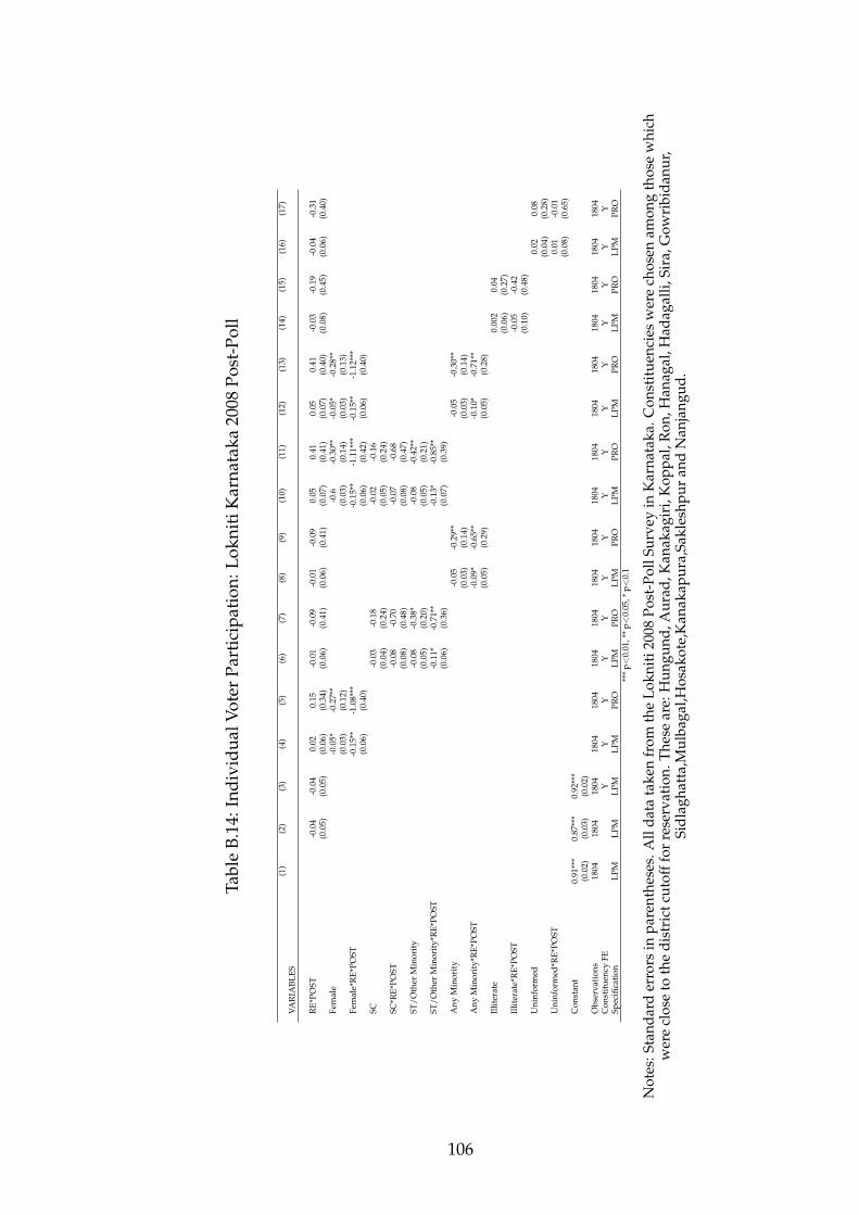
Tabl

eB.

14:I

ndiv

idua

lVot

erPa

rtic

ipat

ion:

Lokn

itiK

arna

taka

2008

Post

-Pol

l

(1)

(2)

(3)

(4)

(5)

(6)

(7)

(8)

(9)

(10)

(11)

(12)

(13)

(14)

(15)

(16)

(17)

VAR

IABL

ES

RE*

POST

-0.0

4-0

.04

0.02

0.15

-0.0

1-0

.09

-0.0

1-0

.09

0.05

0.41

0.05

0.41

-0.0

3-0

.19

-0.0

4-0

.31

(0.0

5)(0

.05)

(0.0

6)(0

.34)

(0.0

6)(0

.41)

(0.0

6)(0

.41)

(0.0

7)(0

.41)

(0.0

7)(0

.40)

(0.0

8)(0

.45)

(0.0

6)(0

.40)

Fem

ale

-0.0

5*-0

.27*

*-0

.6-0

.30*

*-0

.05*

-0.2

8**

(0.0

3)(0

.12)

(0.0

3)(0

.14)

(0.0

3)(0

.13)

Fem

ale*

RE*

POST

-0.1

5**

-1.0

8***

-0.1

5**

-1.1

1***

-0.1

5**

-1.1

2***

(0.0

6)(0

.40)

(0.0

6)(0

.42)

(0.0

6)(0

.40)

SC-0

.03

-0.1

8-0

.02

-0.1

6(0

.04)

(0.2

4)(0

.05)

(0.2

4)SC

*RE*

POST

-0.0

8-0

.70

-0.0

7-0

.68

(0.0

8)(0

.48)

(0.0

8)(0

.47)

ST/O

ther

Min

orit

y-0

.08

-0.3

8*-0

.08

-0.4

2**

(0.0

5)(0

.20)

(0.0

5)(0

.21)

ST/O

ther

Min

orit

y*R

E*PO

ST-0

.11*

-0.7

1**

-0.1

3*-0

.85*

*(0

.06)

(0.3

6)(0

.07)

(0.3

9)A

nyM

inor

ity

-0.0

5-0

.29*

*-0

.05

-0.3

0**

(0.0

3)(0

.14)

(0.0

3)(0

.14)

Any

Min

orit

y*R

E*PO

ST-0

.09*

-0.6

5**

-0.1

0*-0

.71*

*(0

.05)

(0.2

9)(0

.05)

(0.2

8)Il

liter

ate

0.00

20.

04(0

.06)

(0.2

7)Il

liter

ate*

RE*

POST

-0.0

5-0

.42

(0.1

0)(0

.48)

Uni

nfor

med

0.02

0.08

(0.0

4)(0

.28)

Uni

nfor

med

*RE*

POST

0.01

-0.0

1(0

.08)

(0.6

5)C

onst

ant

0.91

***

0.87

***

0.92

***

(0.0

2)(0

.03)

(0.0

2)O

bser

vati

ons

1804

1804

1804

1804

1804

1804

1804

1804

1804

1804

1804

1804

1804

1804

1804

1804

1804

Con

stit

uenc

yFE

YY

YY

YY

YY

YY

YY

YY

YSp

ecifi

cati

onLP

MLP

MLP

MLP

MPR

OLP

MPR

OLP

MPR

OLP

MPR

OLP

MPR

OLP

MPR

OLP

MPR

O**

*p<

0.01

,**

p<

0.05

,*p<

0.1

Not

es:S

tand

ard

erro

rsin

pare

nthe

ses.

All

data

take

nfr

omth

eLo

knit

i200

8Po

st-P

ollS

urve

yin

Kar

nata

ka.C

onst

itue

ncie

sw

ere

chos

enam

ong

thos

ew

hich

wer

ecl

ose

toth

edi

stri

ctcu

toff

for

rese

rvat

ion.

Thes

ear

e:H

ungu

nd,A

urad

,Kan

akag

iri,

Kop

pal,

Ron

,Han

agal

,Had

agal

li,Si

ra,G

owri

bida

nur,

Sidl

agha

tta,

Mul

baga

l,Hos

akot

e,K

anak

apur

a,Sa

kles

hpur

and

Nan

jang

ud.

106

Appendix C

Data Appendix: Chapter 1

I use three chief sources to arrive at descriptive statistics or controls in the main

regressions: the Primary Census Abstracts from the 2001 Census of India; constituency-

level electoral data for the State Legislative Assembly Elections from the Election

Commission of India (Chhatisgarh, Madhya Pradesh and Rajasthan: 2003 and 2008;

Karnataka:2004 and 2008) and individual voting data from the 2008 Karnataka Post-

Poll Survey, released by Lokniti and the Centre for the Study of Developing Soci-

eties.

To arrive at constituency controls, I match each village or town in a district to

a constituency (Concordance available on request). The 2008 round of delimitation

stated explicitly that every constituency would be wholly contained in one district.

The Delimitation guidelines set out the extent of each constituency. I match every

unit (village, town, ward or other administrative unit) to its corresponding con-

stituency, and then assign it to its ”2008” district. This might be of some concern

if new districts are created by merging parts of others together, or other substan-

tial redrawing of boundaries. For the most part, however (and certainly within my

sample), new districts are created by splitting an existing district into two or three,

so each district in 2008 has exactly one analogue in previous years. I am taking the

extent of each constituency as laid out in the 2008 Delimitation document. I do not

find evidence of any other substantial redefinition of constituency limits. I assume

that gerrymandering, where it exists, is either limited or not biased towards either

107

reserved or unreserved constituencies. This is borne out by the survey carried out

by Iyer and Shivakumar (2009), who find that Delimitation arranged constituencies

to even out the population of each constituency, without visible party or political

bias.

In the individual-level voting data from Lokniti, I remove missing observations:

those who were too young to vote in 2004 or 2008, or do not remember whether they

voted in either year.

108

Appendix D

Proofs of Propositions: Chapter 2

D.1 Proof of Proposition 1

Proof of Proposition 1. I consider in turn an interior h and then h = c−1(1) and h = 0.

• Consider first ¯h(I0) = 0.

u( f (h)(1− c(h′)))− (1− π)u( f (h)) = −π I

=⇒ πu( f (h)) = −π I

=⇒ h = 0&I = 0&π = 0

=⇒ h > 0∀h > 0, ∀I1 > I0

=⇒ h ≥ 0, h = 0

• Next, consider ¯h(I0) = c−1(1)

u( f (h)(1− c(h)))− (1− π)u( f (h)) ≥ −π I

=⇒ −(1− π)u( f (h)) ≥ −π I

=⇒ ¯h(I1) ≥ c−1(1)∀I1 > I0

• Finally consider an interior h i.e. 0 < h < c−1(1). If h = c−1[1 − 1/ f (h) ·

109

u−1((1− π) · u( f (h))− π · I)]:

∂h∂I

= (c−1)′[1− 1f (h)

· u−1((1− π) · u( f (h))− π · I)]

·[− 1f (h)

· (u−1)′((1− π) · u( f (h))− π · I)] · (−π) > 0

• To prove concavity of interior h: if (c−1)′(.) > 0, (c−1)′′(.) < 0, (u−1)′(.) >

0, (u−1)′′(.) > 0

∂2h∂I2 = (c−1)′′[1− 1

f (h)· (u−1)′((1− π) · u( f (h))− π · I)]

·[(u−1)′((1− π) · u( f (h))− π · I)]2 · π2

( f (h))2

+(c−1)′[1− 1f (h)

· u−1((1− π) · u( f (h))− π · I)]

·(u−1)′′((1− π) · u( f (h))− π · I)] · −π2

f (h)≤ 0

• If ¯h(I0) = 0, ¯h(I1) ∈ {0, c−1[1− 1f (h) · u

−1((1− π) · u( f (h))− π · I)], c−1(1)}


Proof of Proposition 2. I consider in turn an interior h and then h = c−1(1) and h = 0.

• Consider first ¯h(π0) = 0.

u( f (h)(1− c(h′)))− (1− π)u( f (h)) = −π I

=⇒ πu( f (h)) = −π I

=⇒ h = 0&I = 0∨ π = 0

=⇒ h = 0, π = 0

=⇒ h > 0∀π1 > π0

110

• Next, consider ¯h(π0) = c−1(1)

u( f (h)(1− c(h)))− (1− π)u( f (h)) ≥ −π I

=⇒ −(1− π)u( f (h)) ≥ −π I

=⇒ ¯h(π1) ≥ c−1(1)∀π1 > π0

• Finally consider an interior h i.e. 0 < h < c−1(1). If h = c−1[1 − 1/ f (h) ·

u−1((1− π) · u( f (h))− π · I)]:

∂h∂π

= (c−1)′[1− 1f (h)

· u−1((1− π) · u( f (h))− π · I)]

·[− 1f (h)

· (u−1)′((1− π) · u( f (h))− π · I)] · (−u( f (h))− I) > 0

• To prove concavity of interior h: if (c−1)′(.) > 0, (c−1)′′(.) < 0, (u−1)′(.) >

0, (u−1)′′(.) > 0

∂2h∂π2 = (c−1)′′[1− 1

f (h)· (u−1)′((1− π) · u( f (h))− π · I)]

·[(u−1)′((1− π) · u( f (h))− π · I)]2 · (u( f (h)) + I)2

( f (h))2

+(c−1)′[1− 1f (h)

· u−1((1− π) · u( f (h))− π · I)]

·(u−1)′′((1− π) · u( f (h))− π · I)] · −(u( f (h)) + I)2

f (h)≤ 0

• If ¯h(I0) = 0, ¯h(I1) ∈ {0, c−1[1− 1f (h) · u

−1((1− π) · u( f (h))− π · I)], c−1(1)}


Proof of Proposition 3. I consider in turn h = 0, h = c−1(1) and interior h.

• Consider first c(h) = 1, h1 > h0 > 0, I > 0. Keeping I constant, if surplus over

111

autarky at h0, c(h′(h0)) is the same as that at h1, c(h′(h1)):

u( f (h1)(1− c(h′(h1))))− (1− π) · u( f (h1)) = −π · I

= u( f (h0)(1− c(h′(h0))))

−(1− π) · u( f (h0))

= −(1− π) · u( f (h0))

c(h) = 1 =⇒ u( f (h1)(1− c(h′(h1)))) > 0

=⇒ c(h′(h1)) < c(h′(h0))

=⇒ h′(h1) < h′(h0)

• Consider next I=0. Then:

u( f (h)(1− c(h′)))− (1− π)u( f (h)) = −π · I =⇒ h = 0∨ h′ = 0

• Consider finally h1 > h0 > 0. 0 < h1 < c−1(1). Keeping I constant, if sur-

plus over autarky at h0, c(h′(h0)) is the same as that at h1, c(h′(h1)). f ′(h) >

0, f ′′(h) ≤ 0, c′(h) > 0, c′′(h) > 0, therefore:

h(h1) ≥ h(h0) =⇒ u( f (h1)(1− c(h(h1))))− (1− π) · u( f (h1))

< u( f (h0)(1− c(h(h0))))− (1− π) · u( f (h0))

112


Proof of Proposition 4. Note that with the assumptions of stationarity above (i.e. that

the lowest acceptable transfer of human capital at I is h), one can rewrite the parent’s

decision problem as:

U(h′) = maxh′

u( f (h)(1− c(h′)))

+λ{(1− π) · u( f (h′)) + π · u( f (h′)− I)

+βu( f (h′)(1− c(h′)))− u( f (h′)) + β · π · I}

i.e. If ∃h′ at which the child finds it (weakly) optimal to honestly insure the

parent and then choose insurance herself, her child will also find it weakly optimal

to accept h′′ = h′.

First Order Conditions with respect to h′ suggest that:

λ =u′( f (h)(1− c(h′))) f (h)c′(h′)

π · u′( f (h′)− θ · I) f ′(h′)− π · u′( f (h′)) + β ∂∂h′u( f (h′)(1− c(h′)))

> 0 (D.1)

The denominator is the partial derivative of the child’s surplus over cheating

when h′ = h′′, which, by assumption, is positive.

If constrained first-best is achieved, then keeping λ constant and taking the par-

tial derivative with respect to I:

∂h′

∂I=

AB + C + D + E + F + G + H + J

∈ (0, 1)

Where

A = θ · λπ · u′′( f (h′)− θ · I) f ′(h′) < 0

B = − f (h)c′′(h′)u′( f (h)(1− c(h′)))

C = ( f (h)c′(h′))2 · u′′( f (h)(1− c(h′)))

D = −λ · π · u′( f (h′)) f ′′(h′)

E = −λ · π · u′′( f (h′))( f ′(h′))2

F = λ · π · u′( f (h′)− θ · I) f ′′(h′)

113

G = λ · π · u′′( f (h′)− θ · I)( f ′(h′))2

H = λ · β · u′( f (h′)(1− c(h′))( f ′′(h′)− 2 f ′(h′)c′(h′)− f ′(h′)c′′(h′))

J = λ · β · u′′( f (h′)(1− c(h′))( f ′(h′)(1− c(h′)))2

Since u′(.) > 0, u′′(.) < 0, f ′(.) > 0, f ′′(.) < 0, c′(.) > 0, c′′(.) < 0


Proof of Proposition 5. If constrained first-best is achieved, then keeping λ constant

and taking the partial derivative with respect to θ, from Equation D.1:

∂h′

∂θ=

AB + C + D + E + F + G + H + J

∈ (0, 1)

Where

A = I · λπ · u′′( f (h′)− θ · I) f ′(h′) < 0

B = − f (h)c′′(h′)u′( f (h)(1− c(h′)))

C = ( f (h)c′(h′))2 · u′′( f (h)(1− c(h′)))

D = −λ · π · u′( f (h′)) f ′′(h′)

E = −λ · π · u′′( f (h′))( f ′(h′))2

F = λ · π · u′( f (h′)− θ · I) f ′′(h′)

G = λ · π · u′′( f (h′)− θ · I)( f ′(h′))2


J = λ · β · u′′( f (h′)(1− c(h′))( f ′(h′)(1− c(h′)))2

Since u′(.) > 0, u′′(.) < 0, f ′(.) > 0, f ′′(.) < 0, c′(.) > 0, c′′(.) < 0


Proof of Proposition 6. If constrained first-best is achieved, then keeping λ constant

and taking the partial derivative with respect to π, using Equation D.1:

∂h′

∂π=

A′

B′ + C′ + D′ + E′ + F′ + G′ + H′ + J′

114

Where

A = λ f ′(h′)[u′( f (h′))− u′( f (h′)− θ I)] < 0

B = − f (h)c′′(h′)u′( f (h)(1− c(h′)))

C = ( f (h)c′(h′))2 · u′′( f (h)(1− c(h′)))

D = −λ · π · u′( f (h′)) f ′′(h′)

E = −λ · π · u′′( f (h′))( f ′(h′))2

F = λ · π · u′( f (h′)− θ · I) f ′′(h′)

G = λ · π · u′′( f (h′)− θ · I)( f ′(h′))2


J = λ · β · u′′( f (h′)(1− c(h′))( f ′(h′)(1− c(h′)))2

Since u′(.) > 0, u′′(.) < 0, f ′(.) > 0, f ′′(.) < 0, c′(.) > 0, c′′(.) < 0

115

Appendix E

Figures: Chapter 2

Figure E.1 Maximum Human Capital Transferred to Child: h=.18

0.2

.4.6

.81

Ma

xim

um

Hu

ma

n C

ap

ital T

ran

sfe

rre

d b

y P

are

nt

0 .2 .4 .6 .8 1Cost of Sickness

Maximum Human Capital Transferred by Parenth=0.18

116

Figure E.2 Maximum Human Capital Transferred to Child: h=.5

0.2

.4.6

.8M

axi

mu

m H

um

an

Ca

pita

l Tra

nsf

err

ed

by

Pa

ren

t

0 .2 .4 .6 .8 1Cost of Sickness

Maximum Human Capital Transferred by Parenth=0.5

117

Figure E.3 Maximum Human Capital Transferred to Child: I=0.01

0.2

.4.6

.81

Maxim

um H

uman

Cap

ital O

ffere

d by P

aren

t0 .2 .4 .6 .8 1

Parental Human Capital

Maximum Human Capital Offered by ParentI=0.01


.5.6

.7.8

.91

Maxim

um H

uman

Cap

ital O

ffere

d by P

aren

t

0 .2 .4 .6 .8 1Parental Human Capital



.7.8

.91

Maxim

um H

uman

Cap

ital O

ffere

d by P

aren

t

0 .2 .4 .6 .8 1Parental Human Capital


118

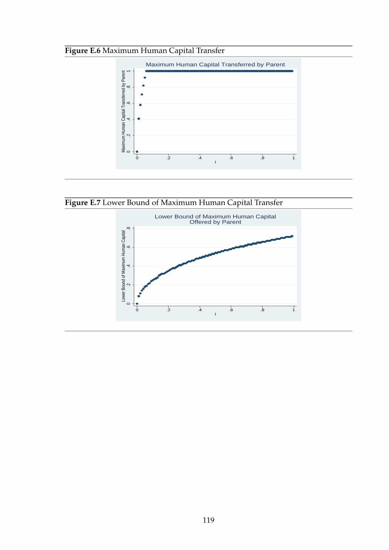
Figure E.6 Maximum Human Capital Transfer

0.2

.4.6

.81

Max

imum

Hum

an C

apita

l Tra

nsfe

rred

by P

aren

t

0 .2 .4 .6 .8 1I

Maximum Human Capital Transferred by Parent

Figure E.7 Lower Bound of Maximum Human Capital Transfer

0.2

.4.6

.8Lo

wer

Bou

nd o

f Max

imum

Hum

an C

apita

l

0 .2 .4 .6 .8 1I

Lower Bound of Maximum Human CapitalOffered by Parent

119

Figure E.8 Minimum Human Capital Transfer Accepted by Child

0.0

5.1

.15

.2M

inim

um H

uman

Cap

ital A

ccep

ted

by C

hild

0 .2 .4 .6 .8 1I

Minimum Human Capital Accepted by Child

120

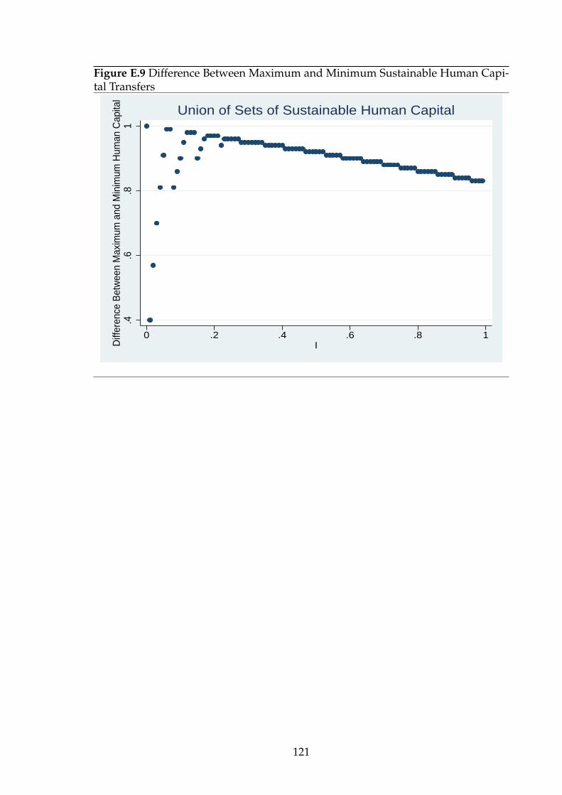
Figure E.9 Difference Between Maximum and Minimum Sustainable Human Capi-tal Transfers

.4.6

.81

Diff

eren

ce B

etw

een

Max

imum

and

Min

imum

Hum

an C

apita

l

0 .2 .4 .6 .8 1I

Union of Sets of Sustainable Human Capital

121

Appendix F

Figures: Chapter 3

Figure F.1 Cross Country Variation in Growth of High-skilled Wage Bill Shares andICT Intensity, 1980- 2004

AustriaDenmark

Finland

FranceGermany

Italy

JapanNetherlands

Spain

UK

USA

-50

51

01

52

0C

ha

ng

e H

igh

-ski

lled

Wa

ge

bill

Sh

are

.005 .01 .015 .02 .025 .03 .035Change ICT/VA

High-skilled Wage Bill Share

122

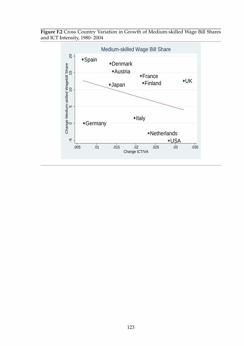
Figure F.2 Cross Country Variation in Growth of Medium-skilled Wage Bill Sharesand ICT Intensity, 1980- 2004

AustriaDenmark

FinlandFrance

GermanyItaly

Japan

Netherlands

Spain

UK

USA-50

51

01

52

0C

ha

ng

e M

ed

ium

-ski

lled

Wa

ge

bill

Sh

are

.005 .01 .015 .02 .025 .03 .035Change ICT/VA

Medium-skilled Wage Bill Share

123

Figure F.3 Cross Country Variation in Growth of Low-skilled Wage Bill Shares andICT Intensity, 1980- 2004

AustriaDenmark

Finland

France

Germany Italy

Japan

Netherlands

SpainUK

USA-3

0-2

5-2

0-1

5-1

0-5

Ch

an

ge

Lo

w-s

kille

d W

ag

eb

ill S

ha

re

.005 .01 .015 .02 .025 .03 .035Change ICT/VA

Low-Skilled Wage Bill Share

124

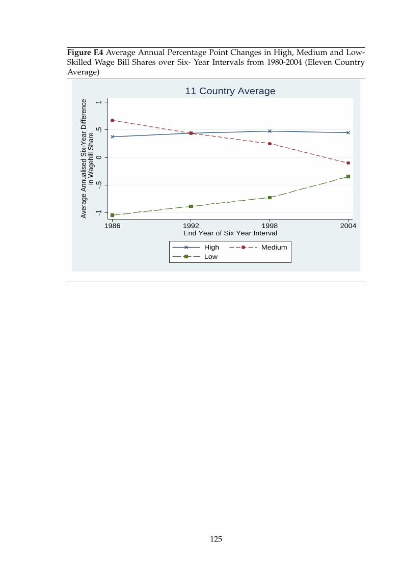
Figure F.4 Average Annual Percentage Point Changes in High, Medium and Low-Skilled Wage Bill Shares over Six- Year Intervals from 1980-2004 (Eleven CountryAverage)

-1-.5

0.5

1

Ave

rage

Ann

ualis

ed S

ix-Y

ear D

iffer

ence

in W

ageb

ill S

hare

1986 1992 1998 2004End Year of Six Year Interval

High MediumLow

11 Country Average

125

Figure F.5 Average Annual Percentage Point Changes in High, Medium and Low-Skilled Wage Bill Shares over Six- Year Intervals from 1980-2004 (U.S. Average)

-1-.5

0.5

1

Ave

rage

Ann

ualis

ed S

ix-Y

ear D

iffer

ence

in W

ageb

ill S

hare

1986 1992 1998 2004End Year of Six Year Interval

High MediumLow

USA Average

126

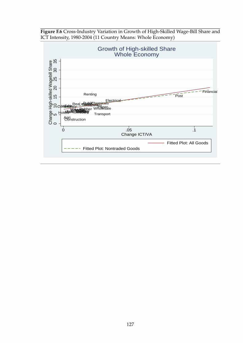
Figure F.6 Cross-Industry Variation in Growth of High-Skilled Wage-Bill Share andICT Intensity, 1980-2004 (11 Country Means: Whole Economy)

Agri

FoodTextilesWoodPaper

Chemicals

RubberMineralsMetals

MachineryElectrical

Transport

ManufacturingSale_motorWholesale

RetailTransport

Post

Real estate

Renting

Construction

Hotels

Financial

PublicEduHealthCommunity

05

1015

2025

3035

Cha

nge

Hig

h-sk

illed

Wag

ebill

Sha

re

0 .05 .1Change ICT/VA

Fitted Plot: All GoodsFitted Plot: Nontraded Goods

Growth of High-skilled ShareWhole Economy

127

Figure F.7 Cross-Industry Variation in Growth of High-Skilled Wage-Bill Share andICT Intensity, 1980-2004 (11 Country Means: Traded Goods Only)

Agri

FoodTextilesWood

Paper

Chemicals


Machinery

Electrical

Transport

Manufacturing

05

1015

20C

hang

e H

igh-

skill

ed W

ageb

ill S

hare

0 .01 .02 .03 .04Change ICT/VA

Growth of High-skilled ShareTraded Goods Only

128

Figure F.8 Cross-Industry Variation in Growth of Medium-Skilled Wage-Bill Shareand ICT Intensity, 1980-2004 (11 Country Means: Whole Economy)

Agri

FoodTextilesWood

PaperChemicals


MachineryElectrical

Transport

Manufacturing

Sale_motorWholesale

Retail

Transport

PostReal estate

Renting

Construction

Hotels

Financial

Public

Edu

Health

Community

05

1015

2025

3035

Cha

nge

Med

ium

-ski

lled

Wag

ebill

Sha

re



Growth of Medium-skilled ShareWhole Economy

129

Figure F.9 Cross-Industry Variation in Growth of Medium-Skilled Wage-Bill Shareand ICT Intensity, 1980-2004 (11 Country Means: Traded Goods Only)

Agri

Food

TextilesWood

Paper

Chemicals

RubberMinerals

Metals

Machinery

Electrical

Transport

Manufacturing

510

1520

25C

hang

e M

ediu

m-S

kille

d W

ageb

ill S

hare

0 .01 .02 .03 .04Change ICT/VA

Growth of Medium-Skilled ShareTraded Goods Only

130

Figure F.10 Cross-Industry Variation in Growth of Low-Skilled Wage-Bill Share andICT Intensity, 1980-2004 (11 Country Means: Whole Economy)

AgriFoodTextilesWood

PaperChemicalsRubberMineralsMetalsMachinery ElectricalTransport

Manufacturing

Sale_motor WholesaleRetailTransport Post

Real estateRenting

ConstructionHotels

FinancialPublic

Edu

Health

Community

05

1015

2025

3035

Cha

nge

Low

-ski

lled

Wag

ebill

Sha

re



Growth of Low-skilled ShareWhole Economy

131

Figure F.11 Cross-Industry Variation in Growth of Low-Skilled Wage-Bill Share andICT Intensity, 1980-2004 (11 Country Means: Traded Goods Only)

Agri

FoodTextilesWood

PaperChemicalsRubber

MineralsMetals

Machinery ElectricalTransport

Manufacturing

-30

-25

-20

-15

-10

Cha

nge

Low

-Ski

lled

Wag

ebill

Sha

re

0 .01 .02 .03 .04Change ICT/VA

Growth of Low-Skilled ShareTraded Goods Only

132

Appendix G

Tables: Chapter 3

Table G.1: Mean Standardized Scores by skill group - 1980 US data

High- Middle- Low-Skilled Skilled Skilled

Routine TasksCognitive Set limits, Tolerances -0.32 0.06 0.07

or StandardsManual Finger Dexterity -0.21 0.13 -0.14

Non-routine tasks

Cognitive Quantitative reasoning 0.79 -0.02 -0.43requirements

Direction, Control 0.90 -0.11 -0.32and Planning

Manual Eye-Hand-Foot -0.36 -0.04 0.29coordination

Note: This table reports the mean standardized task measures by skill group, using 1980 US Censusmicro data and the occ8090 classification from Autor, Levy, and Murnane (2003). For each task

measure, the standardized measure is derived by subtracting from each occupation’s task score theweighted mean task score across all occupations, and then dividing the difference by the standard

deviation of the task measure across the 453 occupations.

133

Tabl

eG

.2:T

opoc

cupa

tion

sby

shar

eof

wor

kers

ofdi

ffer

ents

kill

leve

ls,w

ith

task

mea

sure

s

Stan

dard

ised

Task

mea

sure

s

Rou

tine

Non

-rou

tine

Cog

niti

veM

anua

lC

ogni

tive

Man

ual

occ8

090

Occ

upat

ion

Empl

oym

ent

Frac

tion

Frac

tion

Frac

tion

SetL

imit

s,To

lera

nces

Fing

erQ

uant

itat

ive

Dir

ecti

on,C

ontr

olEy

e,H

and

Des

crip

tion

in19

80H

igh-

skill

edM

iddl

e-sk

illed

Low

-ski

lled

and

Stan

dard

sD

exte

rity

Rea

soni

ngR

equi

rem

ents

and

Plan

ning

Foot

Coo

rdin

atio

n

Top

10oc

cupa

tion

sby

shar

eof

high

-ski

lled

wor

kers

84Ph

ysic

ians

460,

260

0.97

0.03

0.00

-0.9

64.

181.

941.

870.

5017

8La

wye

rs53

4,78

00.

950.

050.

00-0

.96

-1.1

11.

05-0

.51

-0.8

085

Den

tist

s13

5,62

00.

940.

060.

001.

474.

731.

99-0

.55

0.89

133

Med

ical

scie

nce

teac

hers

9,86

00.

930.

060.

01-1

.05

-0.9

01.

732.

08-0

.80

126

Soci

alsc

ienc

ete

ache

rs,n

.e.c

.2,

480

0.93

0.04

0.03

-1.0

5-1

.12

2.01

2.33

-0.8

014

6So

cial

wor

kte

ache

rs1,

060

0.92

0.06

0.02

-1.0

5-1

.12

2.01

2.33

-0.8

012

3H

isto

ryte

ache

rs6,

380

0.92

0.06

0.02

-1.0

5-1

.12

1.73

2.17

-0.8

011

8So

ciol

ogy

teac

hers

;Psy

chol

ogy

teac

hers

9,20

00.

920.

060.

02-1

.05

-1.1

22.

012.

33-0

.80

147

The

olog

yte

ache

rs3,

940

0.91

0.07

0.03

-1.0

5-1

.12

1.97

2.27

-0.8

086

Vete

rina

rian

s37

,440

0.91

0.08

0.01

1.00

4.06

0.96

-0.5

2-0

.71

Top

10oc

cupa

tion

sby

shar

eof

mid

dle-

skill

edw

orke

rs

314

Sten

ogra

pher

s10

6,36

00.

070.

880.

051.

401.

13-0

.58

-0.6

4-0

.80

529

Tele

phon

ein

stal

lers

and

repa

irer

s27

3,98

00.

030.

870.

101.

451.

380.

47-0

.60

2.16

383

Bank

telle

rs63

9,18

00.

070.

860.

071.

482.

530.

29-0

.49

-0.8

031

3Se

cret

arie

s5,

020,

140

0.08

0.86

0.07

-0.7

12.

730.

17-0

.61

-0.7

938

5D

ata-

entr

yke

yers

472,

880

0.05

0.85

0.10

1.31

0.23

0.08

0.16

-0.7

620

6R

adio

logi

cte

chni

cian

s11

0,06

00.

100.

850.

041.

510.

981.

13-0

.59

0.92

527

Tele

phon

elin

ein

stal

lers

and

repa

irer

s65

,560

0.03

0.85

0.12

1.32

1.06

0.34

-0.3

71.

8031

5Ty

pist

s96

9,04

00.

050.

840.

11-0

.06

1.50

-0.1

2-0

.63

-0.7

633

8Pa

yrol

land

tim

ekee

ping

cler

ks20

0,94

00.

060.

830.

111.

470.

790.

05-0

.52

-0.8

052

5D

ata

proc

essi

ngeq

uipm

entr

epai

rers

48,1

400.

100.

830.

061.

431.

190.

81-0

.34

-0.7

0

Top

10oc

cupa

tion

sby

shar

eof

low

-ski

lled

wor

kers

407

Priv

ate

hous

ehol

dcl

eane

rsan

dse

rvan

ts56

9,98

00.

020.

270.

71-1

.05

-1.1

2-0

.86

-0.5

80.

5448

8G

rade

rsan

dso

rter

s,ag

ricu

ltur

alpr

oduc

ts40

,100

0.01

0.30

0.69

-0.0

4-0

.42

-0.8

7-0

.49

0.78

404

Coo

ks,p

riva

teho

useh

old

18,4

600.

030.

300.

67-1

.05

-1.1

2-0

.80

-0.3

8-0

.14

747

Pres

sing

mac

hine

oper

ator

s14

5,74

00.

010.

330.

67-0

.91

0.16

-1.4

7-0

.66

0.42

405

Hou

seke

eper

san

dbu

tler

s10

1,22

00.

020.

320.

65-1

.05

-1.1

2-0

.83

0.04

0.28

738

Win

ding

and

twis

ting

mac

hine

oper

ator

s14

0,08

00.

010.

350.

650.

510.

69-1

.46

-0.6

1-0

.11

403

Laun

dere

rsan

dIr

oner

s3,

160

0.02

0.34

0.65

-1.0

5-1

.12

-1.4

9-0

.66

0.25

479

Farm

wor

kers

1,33

7,02

00.

030.

330.

64-0

.03

-0.3

9-0

.87

-0.4

90.

7844

3W

aite

rs’/

wai

tres

ses’

assi

stan

ts42

2,80

00.

010.

360.

62-1

.01

-0.9

8-1

.34

-0.6

40.

7344

9M

aids

and

hous

emen

969,

720

0.01

0.36

0.62

-0.9

8-1

.05

-1.3

3-0

.47

0.38

Not

e:Th

ista

ble

repo

rts

the

top

10oc

cupa

tion

sfo

rea

chof

the

thre

esk

illca

tego

ries

,alo

ngw

ith

mea

nst

anda

rdiz

edta

skm

easu

res,

usin

g19

80U

SC

ensu

sm

icro

data

and

the

occ8

090

clas

sific

atio

nfr

omA

utor

,Lev

y,an

dM

urna

ne(2

003)

.Fo

rea

chta

skm

easu

re,t

hest

anda

rdiz

edm

easu

reis

deri

ved

bysu

btra

ctin

gfr

omea

choc

cupa

tion

’sta

sksc

ore

the

wei

ghte

dm

ean

task

scor

eac

ross

allo

ccup

atio

ns,a

ndth

endi

vidi

ngth

edi

ffer

ence

byth

est

anda

rdde

viat

ion

ofth

eta

skm

easu

reac

ross

the

453

occu

pati

ons.

134

Tabl

eG

.3:S

umm

ary

Stat

isti

csby

Cou

ntry

Pane

lA:1

980

leve

lsav

erag

edby

coun

try

(1)

(2)

(3)

(4)

(5)

(6)

(7)

Cou

ntry

(Hig

h-sk

illed

wag

e-bi

llsh

are)

(Med

ium

-ski

lled

wag

e-bi

llsh

are)

(Low

-ski

lled

wag

e-bi

llsh

are)

ln(V

alue

Add

ed)

((IC

Tca

pita

l)/

(Val

ueA

dded

))((

Non

ICT

capi

tal)

/(V

alue

Add

ed))

((Im

port

s+Ex

port

s)/

(Val

ueA

dded

))

Aus

tria

8.8

51.6

39.6

8.0

0.01

20.

227

1.43

Den

mar

k5.

350

.544

.27.

80.

029

0.17

42.

24Fi

nlan

d26

.928

.544

.67.

60.

015

0.19

51.

36Fr

ance

11.2

49.6

39.2

10.1

0.01

10.

158

1.23

Ger

man

y9.

466

.024

.710

.30.

020

0.16

81.

31It

aly

5.8

86.9

7.3

9.7

0.02

10.

174

0.91

Japa

n17

.749

.033

.210

.80.

016

0.23

00.

55N

ethe

rlan

ds21

.662

.116

.38.

80.

012

0.15

53.

39Sp

ain

12.7

9.6

77.7

9.1

0.02

10.

265

0.53

UK

9.2

52.7

38.1

9.8

0.01

90.

180

1.54

USA

28.7

56.0

15.3

11.6

0.01

60.

224

0.54

Mea

n14

.351

.134

.69.

40.

018

0.19

51.

4

Pane

lB:C

hang

esfr

om19

80-2

004

aver

aged

byco

untr

y

Cou

ntry

∆(C

olle

gew

age-

bill

shar

e)∆

(Med

ium

-ski

lled

wag

e-bi

llsh

are)

∆(L

ow-s

kille

dw

age-

bill

shar

e)∆

ln(V

alue

Add

ed)

∆((

ICT

capi

tal)

/(V

alue

Add

ed))

∆((

Non

ICT

capi

tal)

/(V

alue

Add

ed))

∆((

Impo

rts+

Expo

rts)

/(V

alue

Add

ed))

Aus

tria

5.4

15.5

-20.

91.

20.

014

0.01

00.

87D

enm

ark

4.1

17.8

-21.

91.

30.

013

-0.0

111.

26Fi

nlan

d15

.212

.0-2

7.2

1.2

0.02

2-0

.001

0.36

Fran

ce7.

714

.1-2

1.8

1.1

0.02

10.

066

0.99

Ger

man

y6.

30.

1-6

.41.

10.

007

0.02

31.

03It

aly

5.3

1.6

-6.9

1.2

0.02

00.

051

0.55

Japa

n10

.811

.5-2

2.3

1.1

0.01

30.

035

0.33

Net

herl

ands

13.1

-2.9

-10.

11.

30.

023

0.04

13.

01Sp

ain

11.9

19.0

-30.

91.

50.

006

0.05

61.

13U

K16

.512

.6-2

9.1

1.3

0.03

2-0

.031

1.26

USA

13.9

-5.1

-8.8

1.4

0.02

80.

032

0.62

Mea

n10

.08.

7-1

8.8

1.2

0.01

80.

025

1.04

Not

e:Th

eta

ble

repo

rts

mea

nsw

eigh

ted

by19

80sh

are

ofea

chco

untr

y’s

empl

oym

ent.

All

vari

able

sar

em

easu

red

for

the

full

sam

ple,

exce

ptfo

rtr

ade

vari

able

s,m

easu

red

only

for

trad

edgo

ods.

135

Tabl

eG

.4:S

umm

ary

Stat

isti

csby

Indu

stry

:198

0le

vels

1980

leve

lsav

erag

edby

indu

stry

Mea

nw

eigh

t(sh

are

of19

80em

ploy

men

t)ac

ross

coun

trie

s

(1)

(2)

(3)

(4)

(5)

(6)

(7)

(8)

(9)

Cod

eD

escr

ipti

onH

igh-

skill

edM

ediu

m-s

kille

dLo

w-s

kille

dln

(Val

ueA

dded

)((

ICT

capi

tal)

((N

onIC

Tca

pita

l)((

Impo

rts+

Expo

rts)

Full

Trad

edgo

ods

wag

e-bi

llsh

are

wag

e-bi

llsh

are

wag

e-bi

llsh

are

/(V

alue

Add

ed))

/(V

alue

Add

ed))

/(V

alue

Add

ed))

sam

ple

only

Agr

icul

ture

,hun

ting

,5.

939

.754

.49.

490.

002

0.24

60.

730.

100.

28fo

rest

ryan

dfis

hing

Food

prod

ucts

,6.

447

.745

.99.

120.

012

0.34

11.

090.

030.

09be

vera

ges

and

toba

cco

Text

iles,

text

ilepr

oduc

ts,

5.0

45.8

49.2

8.60

0.00

60.

168

2.13

0.03

0.09

leat

her

and

foot

wea

rW

ood

and

prod

ucts

7.8

46.8

45.4

7.53

0.01

00.

232

2.30

0.01

0.03

ofw

ood

and

cork

Pulp

,pap

er,

10.8

51.4

37.8

8.75

0.02

10.

242

0.84

0.02

0.07

pape

rpr

oduc

ts,p

rint

ing

and

publ

ishi

ngC

hem

ical

san

dch

emic

alpr

oduc

ts13

.349

.237

.48.

670.

016

0.37

02.

510.

010.

04R

ubbe

ran

dpl

asti

cspr

oduc

ts9.

049

.141

.97.

810.

010

0.25

50.

420.

010.

02O

ther

non-

met

allic

min

eral

prod

ucts

8.6

47.4

44.0

8.14

0.01

40.

270

0.57

0.01

0.03

Basi

cm

etal

s8.

750

.141

.29.

220.

010

0.26

71.

010.

030.

10an

dfa

bric

ated

met

alpr

oduc

tsM

achi

nery

,9.

855

.734

.58.

920.

017

0.20

91.

590.

030.

08no

tels

ewhe

recl

assi

fied

Elec

tric

alan

dop

tica

lequ

ipm

ent

12.6

54.7

32.7

8.88

0.02

40.

176

3.78

0.03

0.08

Tran

spor

tequ

ipm

ent

10.5

54.9

34.5

8.58

0.01

00.

167

1.35

0.02

0.06

Man

ufac

turi

ng7.

047

.745

.38.

020.

013

0.21

33.

210.

010.

04no

tels

ewhe

recl

assi

fied;

recy

clin

gSa

le,m

aint

enan

cean

dre

pair

6.5

59.6

33.9

8.49

0.01

60.

195

0.02

ofm

otor

vehi

cles

and

mot

orcy

cles

;ret

ails

ale

offu

elW

hole

sale

trad

ean

dco

mm

issi

ontr

ade,

10.2

57.1

32.6

9.70

0.03

20.

247

0.05

exce

ptof

mot

orve

hicl

esan

dm

otor

cycl

esR

etai

ltra

de,e

xcep

tofm

otor

vehi

cles

and

mot

orcy

cles

;8.

358

.133

.69.

550.

011

0.08

40.

09re

pair

ofho

useh

old

good

sTr

ansp

orta

ndst

orag

e6.

153

.740

.29.

560.

020

0.20

00.

04Po

stan

dte

leco

mm

unic

atio

ns8.

160

.531

.48.

650.

143

0.23

80.

02R

eale

stat

eac

tivi

ties

26.8

52.4

20.8

9.85

0.01

40.

891

0.01

Ren

ting

ofm

achi

nery

and

equi

pmen

t29

.351

.219

.59.

530.

051

0.18

00.

05an

dot

her

busi

ness

acti

viti

esC

onst

ruct

ion

7.3

52.1

40.6

9.98

0.00

50.

180

0.08

Hot

els

and

rest

aura

nts

6.2

54.4

39.4

8.78

0.01

30.

136

0.04

Fina

ncia

lint

erm

edia

tion

18.3

65.0

16.6

9.49

0.05

10.

297

0.03

Publ

icad

min

and

defe

nce;

20.8

58.4

20.7

9.96

0.01

70.

171

0.07

com

puls

ory

soci

alse

curi

tyEd

ucat

ion

51.7

38.2

10.1

9.58

0.01

30.

078

0.06

Hea

lth

and

soci

alw

ork

27.0

53.1

19.8

9.58

0.01

10.

119

0.07

Oth

erco

mm

unit

y,18

.450

.131

.59.

070.

038

0.21

50.

04so

cial

and

pers

onal

serv

ices

Not

e:Th

eta

ble

repo

rts

mea

nsw

eigh

ted

by19

80sh

are

ofea

chco

untr

y’s

empl

oym

ent.

All

vari

able

sar

em

easu

red

for

the

full

sam

ple,

exce

ptfo

rtr

ade

vari

able

s,m

easu

red

only

for

trad

edgo

ods.

136

Tabl

eG

.5:S

umm

ary

Stat

isti

csby

Indu

stry

:Cha

nges

from

1980

-200

4

Cha

nges

from

1980

-200

4av

erag

edby

indu

stry

Mea

nw

eigh

t(sh

are

of19

80em

ploy

men

t)ac

ross

coun

trie

s

(1)

(2)

(3)

(4)

(5)

(6)

(7)

(8)

(9)

Cod

eD

escr

ipti

on∆

(Hig

h-sk

illed

∆(M

ediu

m-s

kille

d∆

(Low

-ski

lled

∆ln

(Val

ueA

dded

)∆

((IC

Tca

pita

l)∆

((N

onIC

Tca

pita

l)∆

((Im

port

s+Ex

port

s)Fu

llTr

aded

good

sw

age-

bill

shar

ew

age-

bill

shar

ew

age-

bill

shar

e/

(Val

ueA

dded

))/

(Val

ueA

dded

))/

(Val

ueA

dded

))sa

mpl

eon

ly

Agr

icul

ture

,hun

ting

,5.

121

.8-2

6.9

0.56

0.00

30.

009

0.25

0.10

0.28

fore

stry

and

fishi

ngFo

odpr

oduc

ts,

8.0

15.8

-23.

91.

000.

014

0.01

00.

290.

030.

09be

vera

ges

and

toba

cco

Text

iles,

text

ilepr

oduc

ts,

8.2

17.3

-25.

40.

160.

014

0.02

73.

790.

030.

09le

athe

ran

dfo

otw

ear

Woo

dan

dpr

oduc

ts9.

216

.4-2

5.5

0.93

0.01

00.

020

0.02

0.01

0.03

ofw

ood

and

cork

Pulp

,pap

er,

11.0

10.9

-21.

81.

170.

030

0.04

70.

020.

020.

07pa

per

prod

ucts

,pri

ntin

gan

dpu

blis

hing

Che

mic

als

and

chem

ical

prod

ucts

13.1

9.2

-22.

21.

220.

028

0.07

01.

180.

010.

04R

ubbe

ran

dpl

asti

cspr

oduc

ts9.

814

.0-2

3.8

1.28

0.01

70.

022

0.04

0.01

0.02

Oth

erno

n-m

etal

licm

iner

alpr

oduc

ts9.

515

.3-2

4.9

0.90

0.01

10.

052

0.13

0.01

0.03

Basi

cm

etal

s9.

114

.3-2

3.4

0.97

0.01

30.

009

0.18

0.03

0.10

and

fabr

icat

edm

etal

prod

ucts

Mac

hine

ry,

12.0

8.5

-20.

51.

050.

023

-0.0

030.

980.

030.

08no

tels

ewhe

recl

assi

fied

Elec

tric

alan

dop

tica

lequ

ipm

ent

14.6

6.2

-20.

81.

230.

038

0.05

25.

420.

030.

08Tr

ansp

orte

quip

men

t12

.38.

3-2

0.6

1.11

0.02

00.

080

0.94

0.02

0.06

Man

ufac

turi

ng8.

215

.6-2

3.8

1.05

0.01

00.

004

0.41

0.01

0.04

note

lsew

here

clas

sifie

d;re

cycl

ing

Sale

,mai

nten

ance

and

repa

ir8.

59.

7-1

8.1

1.3

0.0

0.0

0.02

ofm

otor

vehi

cles

and

mot

orcy

cles

;ret

ails

ale

offu

elW

hole

sale

trad

ean

dco

mm

issi

ontr

ade,

10.2

7.7

-17.

81.

420.

030

0.05

50.

05ex

cept

ofm

otor

vehi

cles

and

mot

orcy

cles

Ret

ailt

rade

,exc

epto

fmot

orve

hicl

esan

dm

otor

cycl

es;

8.7

9.1

-17.

81.

290.

016

0.07

90.

09re

pair

ofho

useh

old

good

sTr

ansp

orta

ndst

orag

e7.

013

.5-2

0.5

1.36

0.03

00.

072

0.04

Post

and

tele

com

mun

icat

ions

17.2

1.9

-19.

21.

600.

088

0.11

90.

02R

eale

stat

eac

tivi

ties

12.7

-1.1

-11.

61.

810.

014

-0.0

080.

01R

enti

ngof

mac

hine

ryan

deq

uipm

ent

18.1

-7.1

-11.

02.

160.

020

-0.0

270.

05an

dot

her

busi

ness

acti

viti

esC

onst

ruct

ion

4.0

16.2

-20.

21.

190.

009

0.01

30.

08H

otel

san

dre

stau

rant

s7.

812

.5-2

0.3

1.59

0.00

00.

041

0.04

Fina

ncia

lint

erm

edia

tion

19.6

-8.2

-11.

31.

570.

112

0.00

90.

03Pu

blic

adm

inan

dde

fenc

e;13

.10.

7-1

3.7

1.30

0.01

9-0

.022

0.07

com

puls

ory

soci

alse

curi

tyEd

ucat

ion

11.6

-5.4

-6.1

1.47

0.00

4-0

.010

0.06

Hea

lth

and

soci

alw

ork

11.5

0.8

-12.

21.

700.

003

-0.0

080.

07O

ther

com

mun

ity,

11.2

7.1

-18.

31.

650.

003

0.02

90.

04so

cial

and

pers

onal

serv

ices

Not

e:Th

eta

ble

repo

rts

mea

nsw

eigh

ted

by19

80sh

are

ofea

chco

untr

y’s

empl

oym

ent.

All

vari

able

sar

em

easu

red

for

the

full

sam

ple,

exce

ptfo

rtr

ade

vari

able

s,m

easu

red

only

for

trad

edgo

ods.

137

Table G.6: Changes in Wage Bill Shares: 1980-2004

Panel A:Dependent variable: High-Skilled Wage Bill Share

(1) (2) (3) (4) (5) (6) (7) (8)

∆ ((ICT capital) 72.29*** 64.56*** 46.92*** 163.94*** 139.6*** 128.71***/ (Value Added)) (18.28) (17.31) (14.94) (45.48) (42.74) (32.19)∆ ln(Value Added) 5.42*** 4.76*** 3.26 3.41***

(1.24) (0.95) (2.25) (1.07)∆ ((Non ICT capital) -7.64 -6.45* 0.31 -0.47/ (Value Added)) (4.92) (3.51) (5.59) (2.45)Intercept 10.02*** 8.69*** 2.22 9.12*** 6.42*** 4.04*

(0.57) (0.63) (1.67) (0.86) (1.02) (2.19)Country fixed effects X XSample: All industries X X X XSample: Traded industries X X X XObs. 208 208 208 208 84 84 84 84R-squared 0.09 0.19 0.45 0.19 0.22 0.81

Panel B:Dependent variable: Medium-Skilled Wage Bill Share

(1) (2) (3) (4) (5) (6) (7) (8)

∆ ((ICT capital)) -100.78*** -77.76*** -64.52*** -163.98 -41.59 -288.01***/ (Value Added) (30.21) (25.44) (20.24) (115.77) (84.73) (83.94)∆ ln(Value Added) -13.8*** -15.33*** -15.64*** -7.96**

(2.69) (2.23) (4.27) (3.14)∆ ((Non ICT capital) 9.76 18.01* -10.79 1.57/ (Value Added)) (11.88) (10.25) (14.08) (10.98)Intercept 8.73*** 10.59*** 27.24*** 15.5*** 18.20*** 29.75***


Panel C:Dependent variable: Low-Skilled Wage Bill Share

(1) (2) (3) (4) (5) (6) (7) (8)

∆ ((ICT capital)) 28.55 13.21 17.71 0.50 -97.91 159.65**/ (Value Added) (27.34) (25.66) (16.41) (113.51) (100.71) (79.30)∆ ln(Value Added) 8.43*** 10.62*** 12.45*** 4.61

(2.40) (1.95) (4.24) (3.30)∆ ((Non ICT capital) -2.21 -11.68 10.32 -1.28/ (Value Added)) (9.63) (9.07) (11.91) (11.73)Intercept -18.74*** -19.26*** -29.5*** -24.61*** -24.62*** -33.84***


Robust standard errors in parentheses*** p<0.01, ** p<0.05, * p<0.1

Notes: Coefficients estimated by OLS with robust standard errors in parentheses.Columns (1)-(4) are estimated on all industries and columns (5)-(8) are on the tradable sectors.

Weights in columns (1)-(4): each industry’s 1980 share of each country’s employment.

Weights in columns (5)-(8):each industry’s 1980 share of each country’s employment in traded industries.

138

Table G.7: Changes in Wage Bill Shares: 1980-2004 - Robustness checks

Panel A: Dependent variable: High-Skilled Wage Bill Share

(1) (2) (3) (4) (5) (6) (7) (8) (9) (10)

OLS OLS OLS OLS OLS OLS 2SLS 2SLS 2SLS 2SLS∆ ((ICT capital) 46.92*** 42.09*** 50.98*** 48.79*** 132.84** 66.1 121.63** 103.16** 137.99 65.31/ (Value Added)) (14.94) (14.66) (16.64) (16.20) (52.59) (58.15) (53.43) (48.82) (119.44) (104.60)∆ ln(Value Added) 4.76*** 2.93** 5.79*** 4.4** 0.26 -1.97 4.24*** 4.85*** 4.12*** 5.09***

(0.95) (1.39) (1.31) (1.93) (2.94) (3.79) (1.07) (1.10) (1.30) (1.20)∆ ((Non ICT capital) -6.45* -5.06 -9.25** -8.19 15.41 2.56 -8.47** -9.85** -8.91* -8.54/ (Value Added)) (3.51) (3.99) (4.56) (5.13) (12.99) (12.94) (4.02) (4.33) (5.01) (5.16)1980 High-skilled 0.06 0.04 0.34*wage bill share (0.06) (0.07) (0.19)1980 Medium-skilled 0.12** 0.08 0.6**wage bill share (0.05) (0.07) (0.27)Country fixed effects X X X X X X X XSample All All Continental Continental USA USA All All All All

Europe Europe except USA except USAObs. 208 208 143 143 27 27 208 181 208 181R-squared 0.45 0.47 0.44 0.45 0.21 0.43 0.36 0.38 0.32 0.46F-stat for excluded instrument 10.5 9.6 6.5 8.3in the first stage

Panel B: Dependent variable: Medium-Skilled Wage Bill Share

OLS OLS OLS OLS OLS OLS 2SLS 2SLS 2SLS 2SLS∆ ((ICT capital) -64.52*** -41.72*** -62.13*** -51.41*** -160.15*** -80.06 -73.81 -46.74 -42.8 22.21/ (Value Added)) (20.24) (13.35) (18.79) (14.28) (44.52) (60.97) (56.75) (49.04) (235.73) (224.74)∆ ln(Value Added) -15.33*** -2.73 -16.33*** -4.36 -7.57** 0.45 -15.26*** -16.24*** -15.48*** -16.67***

(2.23) (1.99) (3.13) (2.83) (3.32) (3.64) (2.30) (2.47) (2.27) (2.34)∆ ((Non ICT capital) 18.01* 3.89 21.33 7.82 -16.58 -7.9 18.26* 20.02* 17.42 17.62/ (Value Added)) (10.25) (6.61) (13.38) (9.27) (17.77) (13.85) (10.59) (11.41) (11.34) (12.81)1980 High-skilled -0.55*** -0.48*** -0.72***wage bill share (0.08) (0.08) (0.19)1980 Medium-skilled -0.64*** -0.57*** -0.95***wage bill share (0.07) (0.09) (0.28)Country fixed effects X X X X X X X XSample All All Continental Continental USA USA All All All All

Europe Europe except USA except USAObs. 208 208 143 143 27 27 208 181 208 181R-squared 0.58 0.79 0.59 0.77 0.36 0.68 0.58 0.78 0.58 0.52F-stat for excluded instrument 10.5 9.6 6.5 8.3in the first stage


Notes: Coefficients estimated by OLS with robust standard errors in parentheses. Regressionsweighted by the industry’s 1980 share of each country’s employment. In columns (7) and (8) weinstrument the 25-year difference in ICT Capital/Value Added by the 1980 levels of ICTcapital/Value Added in the USA. In columns (9) and (10) we instrument the 25-year difference inICT Capital/Value Added by the 1980 levels of routine task input using the 1991 Directory ofOccupational Titles (constructed as in Autor, Levy and Murnane (2003)).

139

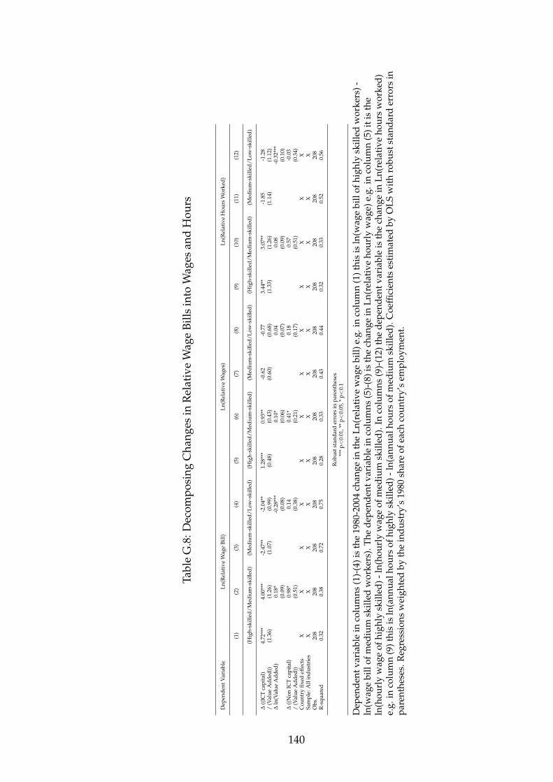
Tabl

eG

.8:D

ecom

posi

ngC

hang

esin

Rel

ativ

eW

age

Bills

into

Wag

esan

dH

ours

Dep

ende

ntV

aria

ble

Ln(R

elat

ive

Wag

eBi

ll)Ln

(Rel

ativ

eW

ages

)Ln

(Rel

ativ

eH

ours

Wor

ked)

(1)

(2)

(3)

(4)

(5)

(6)

(7)

(8)

(9)

(10)

(11)

(12)

(Hig

h-sk

illed

/Med

ium

-ski

lled)

(Med

ium

-ski

lled/

Low

-ski

lled)

(Hig

h-sk

illed

/Med

ium

-ski

lled)

(Med

ium

-ski

lled/

Low

-ski

lled)

(Hig

h-sk

illed

/Med

ium

-ski

lled)

(Med

ium

-ski

lled/

Low

-ski

lled)

∆((

ICT

capi

tal)

4.72

***

4.00

***

-2.4

7**

-2.0

4**

1.28

***

0.93

**-0

.62

-0.7

73.

44**

3.07

**-1

.85

-1.2

8/

(Val

ueA

dded

))(1

.36)

(1.2

6)(1

.07)

(0.9

9)(0

.48)

(0.4

3)(0

.60)

(0.6

8)(1

.33)

(1.2

6)(1

.14)

(1.1

2)∆

ln(V

alue

Add

ed)

0.18

*-0

.28*

**0.

10*

0.04

0.08

-0.3

2***

(0.0

9)(0

.08)

(0.0

6)(0

.07)

(0.0

9)(0

.10)

∆((

Non

ICT

capi

tal)

0.98

*0.

140.

41*

0.18

0.57

-0.0

3/

(Val

ueA

dded

))(0

.51)

(0.3

8)(0

.21)

(0.1

7)(0

.51)

(0.3

4)C

ount

ryfix

edef

fect

sX

XX

XX

XX

XX

XX

XSa

mpl

e:A

llin

dust

ries

XX

XX

XX

XX

XX

XX

Obs

.20

820

820

820

820

820

820

820

820

820

820

820

8R

-squ

ared

0.32

0.38

0.72

0.75

0.28

0.33

0.43

0.44

0.32

0.33

0.52

0.56

Rob

usts

tand

ard

erro

rsin

pare

nthe

ses

***

p<

0.01

,**

p<

0.05

,*p<

0.1

Dep

ende

ntva

riab

lein

colu

mns

(1)-

(4)i

sth

e19

80-2

004

chan

gein

the

Ln(r

elat

ive

wag

ebi

ll)e.

g.in

colu

mn

(1)t

his

isln

(wag

ebi

llof

high

lysk

illed

wor

kers

)-ln

(wag

ebi

llof

med

ium

skill

edw

orke

rs).

The

depe

nden

tvar

iabl

ein

colu

mns

(5)-

(8)i

sth

ech

ange

inLn

(rel

ativ

eho

urly

wag

e)e.

g.in

colu

mn

(5)i

tis

the

ln(h

ourl

yw

age

ofhi

ghly

skill

ed)-

ln(h

ourl

yw

age

ofm

ediu

msk

illed

).In

colu

mns

(9)-

(12)

the

depe

nden

tvar

iabl

eis

the

chan

gein

Ln(r

elat

ive

hour

sw

orke

d)e.

g.in

colu

mn

(9)t

his

isln

(ann

ualh

ours

ofhi

ghly

skill

ed)-

ln(a

nnua

lhou

rsof

med

ium

skill

ed).

Coe

ffici

ents

esti

mat

edby

OLS

wit

hro

bust

stan

dard

erro

rsin

pare

nthe

ses.

Reg

ress

ions

wei

ghte

dby

the

indu

stry

’s19

80sh

are

ofea

chco

untr

y’s

empl

oym

ent.

140

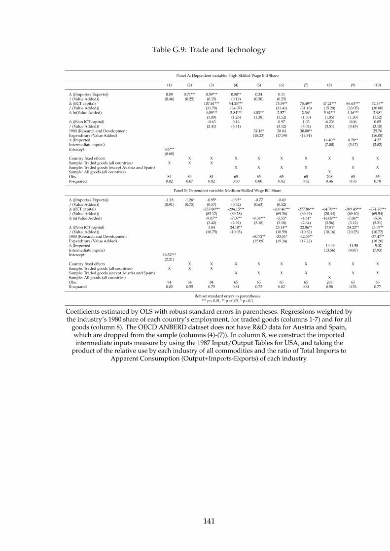
Table G.9: Trade and Technology

Panel A: Dependent variable: High-Skilled Wage Bill Share

(1) (2) (3) (4) (5) (6) (7) (8) (9) (10)

∆ ((Imports+ Exports)) 0.59 0.71*** 0.59*** 0.50** 0.24 0.11/ (Value Added)) (0.46) (0.25) (0.15) (0.19) (0.30) (0.25)∆ ((ICT capital) 107.61*** 94.25*** 73.59** 75.49** 47.21*** 96.63*** 72.37**/ (Value Added)) (31.70) (34.07) (31.41) (31.10) (15.20) (33.05) (30.80)∆ ln(Value Added) 4.09*** 3.84*** 4.03*** 2.57* 2.36* 5.61*** 4.16*** 2.98*

(1.09) (1.26) (1.38) (1.52) (1.35) (1.05) (1.30) (1.52)∆ ((Non ICT capital) -0.63 0.16 0.97 1.03 -6.23* 0.06 0.85/ (Value Added)) (2.41) (3.41) (3.12) (3.02) (3.51) (3.45) (3.18)1980 (Research and Development 34.18* 28.04 30.08** 25.76Expenditure/Value Added) (18.23) (17.59) (14.91) (16.00)∆ (Imported 16.40** 8.78** 4.27Intermediate inputs) (7.00) (3.47) (2.82)Intercept 8.6***

(0.60)Country fixed effects X X X X X X X X XSample: Traded goods (all countries) X X XSample: Traded goods (except Austria and Spain) X X X X X XSample: All goods (all countries) XObs. 84 84 84 65 65 65 65 208 65 65R-squared 0.02 0.67 0.82 0.80 0.80 0.82 0.82 0.46 0.76 0.78

Panel B: Dependent variable: Medium-Skilled Wage Bill Share

∆ ((Imports+ Exports)) -1.18 -1.26* -0.95* -0.95* -0.77 -0.49/ (Value Added)) (0.91) (0.75) (0.57) (0.52) (0.63) (0.52)∆ ((ICT capital) -253.80*** -294.15*** -269.46*** -277.86*** -64.78*** -309.49*** -274.20***/ (Value Added)) (83.12) (69.28) (69.36) (69.49) (20.44) (69.40) (69.54)∆ ln(Value Added) -9.07** -7.07** -9.34*** -5.55* -4.61* -16.08*** -7.06** -5.34

(3.42) (2.92) (3.18) (3.18) (2.64) (2.56) (3.12) (3.31)∆ ((Non ICT capital) 1.84 24.10** 23.14** 22.86** 17.81* 24.22** 23.07**/ (Value Added)) (10.75) (10.03) (10.59) (10.62) (10.16) (10.25) (10.72)1980 (Research and Development -60.72** -33.51* -42.55** -37.47**Expenditure/Value Added) (25.89) (19.24) (17.22) (18.20)∆ (Imported -14.49 -11.58 -5.02Intermediate inputs) (13.56) (9.87) (7.93)Intercept 16.52***

(2.21)Country fixed effects X X X X X X X X XSample: Traded goods (all countries) X X XSample: Traded goods (except Austria and Spain) X X X X X XSample: All goods (all countries) XObs. 84 84 84 65 65 65 65 208 65 65R-squared 0.02 0.55 0.75 0.81 0.73 0.82 0.81 0.58 0.76 0.77


Coefficients estimated by OLS with robust standard errors in parentheses. Regressions weighted bythe industry’s 1980 share of each country’s employment, for traded goods (columns 1-7) and for all

goods (column 8). The OECD ANBERD dataset does not have R&D data for Austria and Spain,which are dropped from the sample (columns (4)-(7)). In column 8, we construct the importedintermediate inputs measure by using the 1987 Input/Output Tables for USA, and taking the

product of the relative use by each industry of all commodities and the ratio of Total Imports toApparent Consumption (Output+Imports-Exports) of each industry.

141

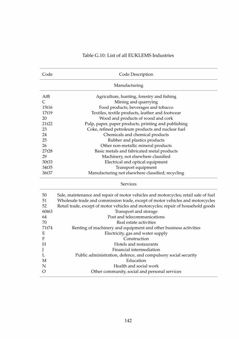
Table G.10: List of all EUKLEMS Industries

Code Code Description

Manufacturing

AtB Agriculture, hunting, forestry and fishingC Mining and quarrying15t16 Food products, beverages and tobacco17t19 Textiles, textile products, leather and footwear20 Wood and products of wood and cork21t22 Pulp, paper, paper products, printing and publishing23 Coke, refined petroleum products and nuclear fuel24 Chemicals and chemical products25 Rubber and plastics products26 Other non-metallic mineral products27t28 Basic metals and fabricated metal products29 Machinery, not elsewhere classified30t33 Electrical and optical equipment34t35 Transport equipment36t37 Manufacturing not elsewhere classified; recycling

Services

50 Sale, maintenance and repair of motor vehicles and motorcycles; retail sale of fuel51 Wholesale trade and commission trade, except of motor vehicles and motorcycles52 Retail trade, except of motor vehicles and motorcycles; repair of household goods60t63 Transport and storage64 Post and telecommunications70 Real estate activities71t74 Renting of machinery and equipment and other business activitiesE Electricity, gas and water supplyF ConstructionH Hotels and restaurantsJ Financial intermediationL Public administration, defence, and compulsory social securityM EducationN Health and social workO Other community, social and personal services

142

Tabl

eG

.11:

List

ofIn

dust

ries

Pool

edby

Cou

ntry

NA

CE

Cod

es

Aus

tria

15t1

6pl

us17

t19

plus

36t3

7;20

plus

21t2

2pl

us24

plus

25pl

us26

plus

27t2

8;29

plus

30t3

3pl

us34

t35;

50pl

us51

plus

52pl

usH

;60t

63;6

4;70

plus

71t7

4;A

tB;F

;J;L

;M;N

;OD

enm

ark

15t1

6;17

t19;

36t3

7;20

;21t

22;2

4;25

;26;

27t2

8;29

;30t

33;3

4t35

;50;

51;5

2;H

;60t

63;6

4;70

;71t

74;A

tB;F

;J;L

;M;N

;OFi

nlan

d15

t16

plus

17t1

9pl

us36

t37;

20pl

us21

t22

plus

24pl

us25

plus

26pl

us27

t28;

29pl

us30

t33

plus

34t3

5;50

plus

51pl

us52

plus

H;6

0t63

;64;

70pl

us71

t74;

AtB

;F;J

;L;M

;N;O

Fran

ce15

t16

plus

17t1

9pl

us36

t37;

20pl

us21

t22

plus

24pl

us25

plus

26pl

us27

t28;

29pl

us30

t33

plus

34t3

5;50

plus

51pl

us52

plus

H;6

0t63

;64;

70pl

us71

t74;

AtB

;F;J

;L;M

;N;O

Ger

man

y15

t16

plus

17t1

9;20

plus

21t2

2pl

us24

plus

25pl

us26

plus

27t2

8pl

us29

;30

t33

plus

34t3

5;36

t37;

50pl

us51

plus

52pl

usH

;60t

63pl

us64

;70

plus

71t7

4;A

tB;F

;J;L

;M;N

;OIt

aly

15t1

6;17

t19;

20;2

1t22

;24;

25;2

6;27

t28;

29;3

0t33

;34t

35;3

6t37

;50;

51;5

2;H

;60

t63;

64;7

0;71

t74;

AtB

;F;J

;L;M

;N;O

Japa

nA

tB;2

0;60

t63;

64;H

;17t

19;2

6;27

t28;

50;2

5pl

us36

t37;

34t3

5;15

t16;

O;2

9;52

;30t

33;F

;21t

22;2

4;71

t74;

51;J

;70;

Lpl

usM

plus

NN

ethe

rlan

dsA

tB;F

;50

plus

51pl

us52

plus

H;6

4;15

t16

plus

17t1

9;60

t63;

20pl

us21

t22

plus

24pl

us25

plus

26pl

us27

t28

plus

36t3

7;J;

29pl

us30

t33

plus

34t3

5;L;

N;7

0pl

us71

t74;

M;O

Spai

n15

t16;

17t1

9;20

plus

21t2

2pl

us24

plus

25pl

us26

plus

27t2

8;29

;30

t33;

34t3

5;36

t37;

50pl

us51

plus

52;6

0t63

;64;

70pl

us71

t74;

AtB

;F;H

;J;L

;M;N

;OU

K64

;F;5

0pl

us51

plus

52pl

usH

;15t

16pl

us17

t19

plus

36t3

7;A

tB;6

0t63

;20

plus

21t2

2pl

us24

plus

25pl

us26

plus

27t2

8;29

plus

30t3

3pl

us34

t35;

O;L

;J;N

;70

plus

71t7

4;M

USA

15t1

6;17

t19;

36t3

7;20

;21t

22;2

4;25

;26;

27t2

8;29

;30t

33;3

4t35

;50;

51;5

2;H

;60

t63;

64;7

0;71

t74;

AtB

;F;J

;L;M

;N;O

143

Tabl

eG

.12:

Trad

e,IC

T,an

dR

esea

rch

and

Dev

elop

men

t

Dep

ende

ntva

riab

le:H

igh-

Skill

edW

age

Bill

Shar

e

(1)

(2)

(3)

(4)

(5)

(6)

(7)

(8)

(9)

(10)

(11)

(12)

(13)

(14)

(15)

(16)

(17)

(18)

∆((

Impo

rts+

Expo

rts)

)0.

59**

*0.

11/

(Val

ueA

dded

))(0

.15)

(0.2

5)∆

((Im

port

s))

1.07

***

0.21

/(V

alue

Add

ed))

(0.3

0)(0

.45)

∆((

Expo

rts)

)1.

16**

*0.

21/

(Val

ueA

dded

))(0

.30)

(0.5

4)∆

((Im

port

sO

ECD

0.68

***

-0.0

5+

Expo

rts

OEC

D))

/(V

alue

Add

ed))

(0.1

8)(0

.37)

∆((

Impo

rts

OEC

D))

1.44

***

-0.4

3/

(Val

ueA

dded

))(0

.52)

(0.9

1)∆

((Ex

port

sO

ECD

))1.

10**

*0.

03/

(Val

ueA

dded

))(0

.30)

(0.6

1)∆

((Im

port

sno

nOEC

D2.

21**

*1.

38+

Expo

rts

nonO

ECD

))/

(Val

ueA

dded

))(0

.58)

(0.7

3)∆

((Im

port

sno

nOEC

D))

2.09

***

1.14

/(V

alue

Add

ed))

(0.6

3)(0

.83)

∆((

Expo

rts

nonO

ECD

))10

.97*

**9.

30**

*/

(Val

ueA

dded

))(3

.38)

(3.4

1)∆

((IC

Tca

pita

l)10

7.61

***

73.5

9**

107.

29**

*73

.22*

*11

0.10

***

74.1

7**

109.

81**

*76

.19*

*11

0.39

***

78.7

5**

112.

20**

*75

.32*

*11

0.43

***

69.9

5**

113.

76**

*71

.89*

*11

6.71

***

67.6

5**

/(V

alue

Add

ed))

(31.

70)

(31.

41)

(31.

52)

(31.

32)

(32.

04)

(31.

41)

(31.

94)

(31.

57)

(31.

55)

(31.

40)

(32.

51)

(31.

53)

(31.

13)

(30.

44)

(32.

06)

(30.

75)

(29.

66)

(29.

74)

∆ln

(Val

ueA

dded

)4.

09**

*2.

57*

4.30

***

2.62

*3.

80**

*2.

50*

3.94

***

2.28

4.09

***

2.01

3.74

***

2.38

4.27

***

3.07

**4.

16**

*2.

86*

3.76

***

3.04

**(1

.09)

(1.5

2)(1

.13)

(1.5

2)(1

.06)

(1.4

9)(1

.09)

(1.5

0)(1

.11)

(1.4

1)(1

.07)

(1.4

8)(1

.12)

(1.4

6)(1

.16)

(1.5

0)(0

.97)

(1.1

8)∆

((N

onIC

Tca

pita

l)-0

.63

0.97

-0.5

00.

99-0

.76

0.95

-0.4

61.

040.

000.

90-0

.82

1.01

-1.1

00.

61-1

.20

0.47

0.24

2.77

/(V

alue

Add

ed))

(2.4

1)(3

.12)

(2.3

8)(3

.11)

(2.4

5)(3

.13)

(2.3

9)(3

.05)

(2.3

3)(2

.98)

(2.4

6)(3

.13)

(2.5

0)(3

.22)

(2.5

1)(3

.24)

(2.4

2)(2

.97)

1980

(Res

earc

han

dD

evel

opm

ent

28.0

428

.05

28.2

730

.89*

32.9

7*29

.83

25.3

826

.73*

25.8

5*Ex

pend

itur

e/V

alue

Add

ed)

(17.

59)

(16.

88)

(18.

06)

(18.

27)

(17.

36)

(18.

33)

(15.

53)

(15.

88)

(13.

84)

Cou

ntry

fixed

effe

cts

XX

XX

XX

XX

XX

XX

XX

XX

XX

Obs

.84

6584

6584

6584

6584

6584

6584

6584

6584

65R

-squ

ared

0.82

0.82

0.82

0.82

0.82

0.82

0.82

0.82

0.82

0.82

0.82

0.82

0.82

0.83

0.82

0.82

0.83

0.83

Rob

usts

tand

ard

erro

rsin

pare

nthe

ses

***

p<

0.01

,**

p<

0.05

,*p<

0.1

Coe

ffici

ents

esti

mat

edby

OLS

wit

hro

bust

stan

dard

erro

rsin

pare

nthe

ses.

Reg

ress

ions

wei

ghte

dby

the

indu

stry

’s19

80sh

are

ofea

chco

untr

y’s

empl

oym

ent,

for

trad

edgo

ods.

The

OEC

DA

NBE

RD

data

setd

oes

noth

ave

R&

Dda

tafo

rA

ustr

iaan

dSp

ain,

whi

char

edr

oppe

dfr

omth

esa

mpl

e(c

olum

ns2,

4,6,

8,10

,12,

14,1

6an

d18

)

144

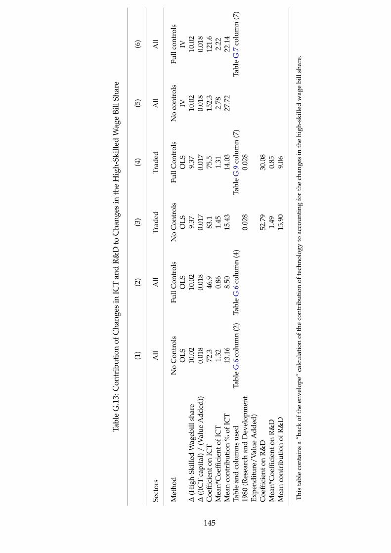
Tabl

eG

.13:

Con

trib

utio

nof

Cha

nges

inIC

Tan

dR

&D

toC

hang

esin

the

Hig

h-Sk

illed

Wag

eBi

llSh

are

(1)

(2)

(3)

(4)

(5)

(6)

Sect

ors

All

All

Trad

edTr

aded

All

All

Met

hod

No

Con

trol

sFu

llC

ontr

ols

No

Con

trol

sFu

llC

ontr

ols

No

cont

rols

Full

cont

rols

OLS

OLS

OLS

OLS

IVIV

∆(H

igh-

Skill

edW

ageb

illsh

are

10.0

210

.02

9.37

9.37

10.0

210

.02

∆((

ICT

capi

tal)

/(V

alue

Add

ed))

0.01

80.

018

0.01

70.

017

0.01

80.

018

Coe

ffici

ento

nIC

T72

.346

.983

.175

.515

2.3

121.

6M

ean*

Coe

ffici

ento

fIC

T1.

320.

861.

451.

312.

782.

22M

ean

cont

ribu

tion

%of

ICT

13.1

68.

5015

.43

14.0

327

.72

22.1

4Ta

ble

and

colu

mns

used

Tabl

eG

.6co

lum

n(2

)Ta

ble

G.6

colu

mn

(4)

Tabl

eG

.9co

lum

n(7

)Ta

ble

G.7

colu

mn

(7)

1980

(Res

earc

han

dD

evel

opm

ent

0.02

80.

028

Expe

ndit

ure/

Val

ueA

dded

)C

oeffi

cien

ton

R&

D52

.79

30.0

8M

ean*

Coe

ffici

ento

nR

&D

1.49

0.85

Mea

nco

ntri

buti

onof

R&

D15

.90

9.06

This

tabl

eco

ntai

nsa

”bac

kof

the

enve

lope

”ca

lcul

atio

nof

the

cont

ribu

tion

ofte

chno

logy

toac

coun

ting

for

the

chan

ges

inth

ehi

gh-s

kille

dw

age

bill

shar

e.

145

Appendix H

Data Appendix: Chapter 3

H.1 Construction of main dataset

Our main dataset is EUKLEMS (http://www.euklems.net/), which is an industry-

level panel dataset created by economic researchers funded by the European Com-

mission. It covers the European Union, the US, Japan, and other countries, and

contains a wealth of information on productivity-related variables. These were con-

structed through joint work with census bureau in each country and are designed to

be internationally comparable. Details of the methodology are in Timmer, van Mo-

ergastel, Stuivenwold, Ypma, O’Mahony, and Kangasniemi (2007), Timmer, Inklaar,

O’Mahony, and van Ark (2010) and Timmer and O’Mahony (2009).

In the construction of our sample we faced a number of technical issues. First,

although college wage bill shares are reported for 30 industries in each country,

these reported wage bill shares are not unique within each country. For example, in

a certain country the reported college wage bill share for industry A and industry

B may be (college wage bill in A + college wage bill in B)/(total wage bill in A +

total wage bill in B). The identity and number of industries pooled together vary

across countries. In order to use as much of variation as possible, we aggregate

industries within each country up to the lowest level of aggregation that ensures

that the college wage bill share is unique across the aggregated observations. This

is also sufficient to ensure that other variables we use, such as our ICT and value

146

added measures, have unique values across observations.

Second, as a measure of ICT intensity we use ICT capital compensation divided

by value added directly from EUKLEMs. ICT capital is built using the Perpetual In-

ventory method based on real ICT investment flows (using a quality-adjusted price

deflator). ICT capital compensation is the stock of ICT capital multiplied by its user

cost. Non-ICT capital compensation is built in the same way1.

Third, matching trade variables into our main dataset required data required

currency conversions, since EUKLEMS reports data in historical local currency and

COMTRADE reports data in historical dollars. To overcome this difference, we con-

vert nominal values to current US Dollars using exchange rates from the IMF IFS

website. To convert national currency to the Euro (for Eurozone countries), we use

exchange rates from the website:

http://ec.europa.eu/economy finance/euro/transition/conversion rates.htm

We use trade figures from the UN’s COMTRADE dataset. Data is downloaded

in the four digit Standard International Trade Classification format (revision 2), and

converted to the European NACE Rev 1 classification used in the EUKLEMS dataset

(concordance available on request). Our trade regressions contain the updated data

from 21st March 2008.

To decompose trade into OECD versus non-OECD, we use the 2007 definition

of OECD countries (Austria, Australia, Belgium, Canada, the Czech Republic, Den-

mark, Finland, France, Germany, Greece, Hungary, Iceland, Ireland, Italy, Japan,

Korea, Luxembourg, Mexico, the Netherlands, New Zealand, Norway, Poland, Por-

tugal, the Slovak Republic, Spain, Sweden, Switzerland, Turkey, the UK and the

USA). This means that Czechoslovakia and Belgium-Luxembourg were treated as

OECD countries in 1980.1Because EUKLEMS calculates capital compensation as a residual in a few cases observations

can have negative capital compensation. Of the 208 country-industry cells we use, negative capitalcompensation occurs in 12 cases in 1980 and in 3 cases in 2004. These are typically agriculture (whichis heavily subsidized and becomes smaller over time) and industries where public services play animportant role (e.g. education and health). To overcome this problem, we bottom-coded negativevalues of ICT and non-ICT capital compensation to zero. Our results are robust to dropping theseobservations from the sample.

147

Finally, we account for the fact that the (aggregated) industries we use differ

substantially in their employment shares within each country’s population. We

therefore use the employment shares of each industry in 1980 (our base year) in

total employment as analytical weights in the regressions using both tradable and

non-tradable industries. For trade regressions, which use only the traded indus-

tries, each industry’s weight is its employment share in the traded industries for

that country, so that the sum of weights for each country is still equal to one.

H.2 Construction of task measures by skill

To construct measures of task content by occupation and education group, which

we use in Tables G.2 and G.1, we begin with US Census micro data for 1980 from

IPUMS, which identify each person’s occupation (using the three-digit 1980 occu-

pation definitions from IPUMS) and education (measured in years of schooling

completed). We assign each person to one of three educational categories - high,

medium, or low - using the EUKLEMS classification for the US. In other words,

high-skill workers are those who have at least 16 years of education, middle-skilled

workers are those with 13-15 years of education, and low-skilled workers are those

with 12 years of education. We then assign to each person the “80-90” occupation

code using the concordance from Autor, Levy, and Murnane (2003), and we match

to each occupation the task measures, which Autor, Levy, and Murnane (2003) de-

rive from the 1991 Dictionary of Occupational Titles. These include routine cog-

nitive tasks (measured using Set limits, Tolerances, or Standards); routine manual

tasks (measured using Finger Dexterity); non-routine cognitive tasks measured us-

ing both (i) Quantitative reasoning requirements and (ii) Direction, Control, and

Planning and non-routine manual tasks (measured using Eye-Hand-Foot coordina-

tion).

We then collapse the data to the occupation-skill level, using 1980 person weights

from IPUMS. Finally, we standardize each of these five task measures by subtracting

148

the mean task score across occupations, weighted by person weights, and dividing

the resulting difference by the standard deviation of the task measure across occu-

pations. The results in Tables G.2 and G.1 discussed below use these standardized

task measures.

We calculate the intensity of occupation O in terms of skill level S ∈ {H, M, L}

as

ShareOS =

EOS

EO,

where EoS is the number of people in occupation O with skill level S, and EO is the

total number of people with occupation O. We then rank the occupations in terms

of their intensity of each of the three skill groups, and Table 1 presents the ten top

occupations in each skill category, and the score of each of these occupations on each

task k.

Finally, we calculate the average score on each task k for each skill level S as

IkS = ∑

O

EOS

ESIko ,

where IkO is occupation O’s score on task k, EoS is the number of people in occupation

O with skill level S, and ES is the total number of people with skill level S. These

scores are reported in Table G.1.

149

Bibliography

ACEMOGLU, D. (2003): “The Effects of Overlapping Majority-Minority Districts onLatino Turnout,” Patterns of Skill Premia, 70(2), 199–230.

ACEMOGLU, D., AND D. AUTOR (2010): Handbook of Labor Economics Volume IVchap.Skills, Tasks and Technologies: Implications for Employment and Earnings.Princeton University Press.

A.J.SAUNDERS (1920–1922): “The Sourashtra Community in Madura, South India,”.

AKER, J. C., P. COLLIER, AND P. C. VICENTE (2011): “Is Information Power? UsingCell Phones during an Election in Mozambique,” .

AKERLOF, G. (1976): “The Economics of Caste and of the Rat Race and Other WoefulTales,” Quarterly Journal of Economics, 90(4), 599–617.

(1980): “.A Theory of Social Custom, of which Unemployment May be OneConsequence.,” Quarterly Journal of Economics, 94(4), 749–775.

ATCHADE, Y. F., AND L. WANTCHEKON (2007): “Does Ethnic Solidarity FacilitateElectoral Support for Nation-Building Policies?: Evidence from a Political Exper-iment,” .

AUTOR, D., AND D. DORN (2009): “Inequality and Specialization: The Growth ofLow-Skill Service Jobs in the United States,” .

AUTOR, D., L. KATZ, AND M. KEARNEY (2006): “The Polarization Of The U.S. LaborMarket,” American Economic Review, 96(2), 189–194.

(2008): “Trends in U.S. Wage Inequality: Revising the Revisionists,” Reviewof Economics and Statistics, 90(2), 300–323.

AUTOR, D., L. KATZ, AND A. KRUEGER (1998): “Computing Inequality: Have Com-puters Changed the Labor Market?,” Quarterly Journal of Economics, 113(4), 1169–1214.

AUTOR, D., F. LEVY, AND R. MURNANE (2003): “The Skill Content Of RecentTechnological Change: An Empirical Exploration,” Quarterly Journal of Economics,118(4), 1279–1333.

BANERJEE, A., M. BERTRAND, S. DATTA, AND S. MULLAINATHAN (2009): “La-bor market discrimination in Delhi: Evidence from a field experiment,” Journal ofComparative Economics, 37, 14–27.

150

BANERJEE, A., E. DUFLO, M. GHATAK, AND J. LAFORTUNE (2009): “Marry ForWhat: Caste and Mate Selection in Modern India,” National Bureau of EconomicResearch Working Paper 14958.

BANERJEE, A., AND R. PANDE (2007): “Parochial Politics: Ethnic Preferences andPolitician Corruption,” C.E.P.R Discussion Paper 6381.

BANNERJEE, A., AND A. NEWMAN (1993): “Occupational Choice and the Process ofDevelopment,” Journal of Political Economy, 96(4), 1225–1252.

BARRETO, M., G. SEGURA, AND N. WOODS (2004): “The Effects of OverlappingMajority-Minority Districts on Latino Turnout,” American Political Science Review,98, 65–75.

BERMAN, E. (2000): “Sect, Subsidy and Sacrifice:an Economist’s View of Ultra-Orthodox Jews,” Quarterly Journal of Economics, 115(3), 905–953.

BERMAN, E., J. BOUND, AND Z. GRILICHES (1994): “Changes in the Demand forSkilled Labor within US Manufacturing Industries: Evidence from the AnnualSurvey of Manufacturing,” Quarterly Journal of Economics, 109(2), 367–397.

(1997): “The Returns to Computer Use Revisited: Have Pencils Changed theWage Structure Too?,” Quarterly Journal of Economics, 112(1), 291–303.

BERMAN, E., R. SOMANATHAN, AND H. TAN (2005): “Is Skill-Biased TechnologicalChange Here Yet? Evidence from Indian Manufacturing in the 1990s,” Annalesd’Economie et de Statistique, 79–80, 299–321.

BERTRAND, M., E. DUFLO, AND S. MULLAINATHAN (2004): “How Much Shouldwe Trust Differences-in-Differences Estimates?,” Quarterly Journal of Economics,119(1), 249–275.

BERTRAND, M., R. HANNA, AND S. MULLAINATHAN (2010): “Affirmative Actionin Education: Evidence from Engineering College Admissions in India,” Journalof Public Economics, 94(1-2), 16–29.

BESLEY, T., AND A. CASE (2003): “Political Insitutions and Policy Choices: EvidenceFrom the United States,” Institute for Fiscal Studies, 02(13).

BESLEY, T., R. PANDE, AND V. RAO (2005): “Participatory democracy in action: sur-vey evidence from South India,” Journal of the European Economic Association, 3(2-3), 648–657.

BLOOM, N., M. DRACA, AND J. V. REENEN (2011): “Trade Induced TechnicalChange? The Impact of Chinese Imports on Technology, Jobs and Plant Survival,”.

BLUNT, E. A. H. (1969): The Caste System of Northern India: with Special Reference tothe United Provinces of Agra and Oudh. S. Chand.

BOND, S., AND J. V. REENEN (2007): Handbook of Econometrics Volume 6Achap. Micro-econometric models of investment and employment.

151

BOUGLE, C. (1971): Essays on the Caste System (Translated by D.F.Pocock). CambridgeUniversity Press.

BROWN, R., AND L. CHRISTENSEN (1981): Modelling and Measuring Natural ResourceSubstitutionchap. Estimating elasticities of substitution in a model of partial staticequilibrium: an application to US agriculture 1947-74. MIT Press, Cambridge.

BUHLER, G. (1886): The Laws of Manu. AMS Press.

CAMERON, C., D. EPSTEIN, AND S. O’HALLORAN (1996): “Do Majority-MinorityDistricts Maximize Substantive Black Representation in Congress?,” American Po-litical Science Review, 90(4), 794–812.

CARD, D. (2009): “Immigration and Inequality,” American Economic Review, 99(2),1–21.

CHANDRA, K. (2003): Why Ethnic Parties Succeed: Patronage and Ethnic Headcounts inIndia. Cambridge University Press.

CHATTOPADHYAY, R., AND E. DUFLO (2004): “Women as Policy Makers: EvidenceFrom a Randomized Policy Experiment in India,” Econometrica, 72(5), 1409–1443.

CHIAPPORI, P.-A., K. SAMPHANTHARAK, S. SCHULHOFER-WOHL, AND R. M.TOWNSEND (2011): “Heterogeneity and Risk Sharing in Village Economies,” Na-tional Bureau of Economic Research Working Paper 16696.

CHIN, A., AND N. PRAKASH (2009): “The Redistributive Effects of Political Reser-vation for Minorities: Evidence from India,” IZA Discussion Paper No. 4391.

CLOTS-FIGUERAS, I. (2007): “Are female leaders good for education? : Evidencefrom India,” Universidad Carlos III, Departamento de Economıa Working Paperwe077342.

COATE, S., AND B. KNIGHT (2007): “Socially Optimal Districting: A Theoretical andEmpirical Exploration,” Quarterly Journal of Economics, 122(4), 1409–1471.

COLLIER, P., AND P. C. VICENTE (2011): “Votes and Violence: Evidence from a FieldExperiment in Nigeria,” .

(2012): “Violence, Bribery, and Fraud: The Political Economy of Elections inSub-Saharan Africa,” Public Choice (forthcoming).

D.N.MAJUMDAR (1958): Caste and Communication in an Indian Village. London: AsiaPublishing House.

DOWNS, A. (1957): An Economic Theory of Democracy. New York: Harper and Row.

DUFLO, E. (2005): “Why Political Reservations?,” Journal of the European EconomicAssociation, 3(2), 668–678.

E.R.LEACH (ed.) (1960): Aspects of Caste in South India, Ceylon and North-West Pak-istanchap. Caste in a Tanjore Village. The Syndics of the Cambridge UniversityPress.

152

ESWARAN, M., AND A. KOTWAL (1985): “A Theory of Two-Tier Labor Markets inAgrarian Economies,” American Economic Review, 75(1), 162–177.

FEDDERSEN, T. J. (2004): “Rational Choice Theory and the Paradox of Not Voting,”Journal of Economic Perspectives, 18(1), 99–112.

FEDDERSEN, T. J., AND W. PESENDORFER (1996): “The Swing Voters’ Curse,” Amer-ican Economic Review, 86(3), 408–424.

FEREJOHN, J. A., AND M. P. FIORINA (1975): “Closeness Counts Only in Horseshoesand Dancing,” American Political Science Review, 69(3), 920–925.

FORD, D., AND R. PANDE (2011): “Gender Quotas and Female Leadership,” Back-ground Paper for World Development Report ,World Bank 2011.

FREITAS, K. (2006): “The Indian Caste System as a Means of Contract Enforcement,”Mimeo, Northwestern University.

FUJIWARA, T. (2010): “Voting Technology, Political Responsiveness, and InfantHealth: Evidence from Brazil,” Job Market Paper.

GEYS, B. (2006): “’Rational’ Theories of Voter Turnout: A Review,” Political StudiesReview, 4(1), 16–35.

GHATAK, M. (1999): “Group Lending, Local Information and Peer Selection,” Jour-nal of Development Economics, 60(1), 27–50.

GHATAK, M., AND T. W. GUINNANE (1999): “The Economics of Lending with JointLiability: Theory and Practice,” Journal of Development Economics, 60(1), 195–228.

GOITEIN, S. D. (1973): Letters of Medieval Jewish Traders, translated from the Arabic withan Introduction and Notes. Princeton University Press.

(1978): A Mediterranean Society: The Family. University of California Press.

GOLDIN, C., AND L. KATZ (2008): The Race between Education and Technology. Har-vard University Press.

GOOS, M., AND A. MANNING (2007): “Lousy and Lovely Jobs: The Rising Polariza-tion of Work in Britain,” Review of Economics and Statistics, 89(1), 118–133.

GOOS, M., A. MANNING, AND A. SALOMONS (2009): “Job Polarization in Europe,”American Economic Review, 99(2), 58–63.

(2011): “Explaining Job Polarization in Europe: The Roles of Technologyand Globalization,” .

GOSNELL, H. F. (1927): Getting Out the Vote: an Experiment in the Stimulation of Vot-ing. University of Chicago Press.

GREIF, A. (1993): “Contract Enforceability and Economic Institutions in Early Trade:The Maghribi Traders’ Coalition,” American Economic Review, 83(3), 525–548.

GRILICHES, Z. (1969): “Capital-Skill complementarity,” Review of Economics andStatistics, 51(4), 465–468.

153

HOROWITZ, D. L. (1985): Ethnic Groups in Conflict. Berkeley: University of Califor-nia Press.

HUSTED, T., AND L. KENNY (1997): “The Effect of the Expansion of the Voting Fran-chise on the Size of the Government,” Journal of Political Economy, 105(1), 54–82.

HUTTON, J. H. (1961): Caste in India. Oxford University Press.

I.R.DAVE (1976): The Saurashtrians of South India. Rajkot.

IYER, L., A. MANI, P. MISHRA, AND P. TOPALOVA (2011): “The Power of PoliticalVoice: Women’s Political Representation and Crime in India,” Working Paper,Harvard Business School.

IYER, L., AND M. SHIVAKUMAR (2009): “Electoral Redistricting in the World’sLargest Democracy: an Evaluation,” Working Paper, Harvard Business School.

JORGENSON, D., M. HO, AND K. STIROH (2008): “A Retrospective Look at the USProductivity Growth Resurgence,” Journal of Economic Perspectives, 22(1), 3–24.

KARVE, I. (1953): Kinship organisation in India. Pooma : Published by Dr S.M. Katrefor the Deccan College Post-graduate and Research Institute.

KRUEGER, A. (1993): “How computers have changed the wage structure,” QuarterlyJournal of Economics, 108(1), 33–60.

KRUGMAN, P. (2008): “Trade and Wages Reconsidered,” .

KUROSAKI, T., AND Y. MORI (May 2011): “Does political reservation affect voterturnout?,” The Hindu,Opinion-Editorial.

LANG, K. (2002): “Of Pencils and Computers,” .

LIZZERI, A., AND N. PERSICO (2004): “Why Did the Elites Extend the Suffrage?Democracy and the Scope of Government, With an Application to Britain’s ”Ageof Reform”,” Quarterly Journal of Economics, 119(2), 705–763.

LUKE, N., AND K. MUNSHI (2006): “New Roles for Marriage in Urban Africa: Kin-ship Networks and the Labor Market in Kenya,” The Review of Economics and Statis-tics, 88(2), 264–282.

MACHIN, S., AND J. V. REENEN (1998): “Technology and Changes in Skill Structure:Evidence from Seven OECD Countries,” Quarterly Journal of Economics, 113(4),1215–1244.

MAZZOLARI, F., AND G. RAGUSA (2008): “Spillovers from High-Skill Consumptionto Low-Skill Labor Markets,” .

M.N.SRINIVAS (1962): Caste in Modern India and Other Essays. Asia PublishingHouse.

MUNSHI, K., AND M. ROSENZWEIG (2006): “Traditional Institutions Meet the Mod-ern World: Caste, Gender, and Schooling Choice in a Globalizing Economy,”American Economic Review, 96(4), 1225–1252.

154

(2008): “The Efficacy of Parochial Politics: Caste, Commitment, and Com-petence in Indian Local Governments,” BREAD Working Paper.

(2009): “Why is Mobility in India so Low? Social Insurance, Inequality, andGrowth,” National Bureau of Economic Research Working Paper 14850.

NAIDU, S. (2009): “Suffrage, Schooling, and Sorting in the Post-Bellum U.S. South,”Job Market Paper.

NALEBUFF, B., AND R. SCHACHAR (1999): “Follow the Leader: Theory and Evi-dence on Political Participation,” American Economic Review, 89(3), 525–547.

NGAI, R., AND C. PISSARIDES (2007): “Structural Change in a Multisector Model ofGrowth,” American Economic Review, 97(1), 429–443.

OGILVIE, S. (2004): “Guilds, efficiency, and social capital: evidence from Germanproto-industry,” Economic History Review, 57(2), 286–333.

O’MALLEY, L. S. S. (1968): Modern India and the West: A Study of the Interaction oftheir Civilizations. Oxford University Press.

ORDESHOOK, P., AND W. RIKER (1968): “A Theory of the Calculus of Voting,” Amer-ican Political Science Review, 62(1), 25–42.

PALFREY, T., AND H. ROSENTHAL (1983): “A Strategic Calculus of Voting,” PublicChoice, 41(1), 7–53.

PANDE, R. (2003): “Can Mandated Political Representation Increase Policy Influ-ence for Disadvantaged Minorities? Theory and Evidence from India,” AmericanEconomic Review, 93(4), 1132–1151.

(2011): “Can Informed Voters Enforce Better Governance? Experiments inLow-Income Democracies,” Annual Review of Economics, 3, 215–237.

SPITZ-OENER, A. (2006): “Technical Change, Job Tasks, and Rising Educational De-mands: Looking Outside the Wage Structure,” Journal of Labor Economics, 24(2),235–270.

TIMMER, M., R. INKLAAR, M. O’MAHONY, AND B. VAN ARK (2010): EconomicGrowth in Europe: A Comparative Industry Perspective. Cambridge University Press.

TIMMER, M., AND M. O’MAHONY (2009): “Output, Input and Productivity Mea-sures at the Industry Level: The EU KLEMS Database,” Economic Journal, 119(538),F374–F403.

TIMMER, M., T. VAN MOERGASTEL, E. STUIVENWOLD, G. YPMA, M. O’MAHONY,AND M. KANGASNIEMI (2007): “EU KLEMS Growth and Productivity AccountsVersion 1.0,” .

TOWNSEND, R. M. (1994): “Risk and Insurance in Village India,” Econometrica, 62(3),539–591.

155

VICENTE, P. C., AND L. WANTCHEKON (2009): “Clientelism and Vote Buying:Lessons from Field Experiments in African Elections,” Oxford Review of EconomicPolicy, 25(2), 292–305.

WANTCHEKON, L. (2003): “Clientelism and Voting Behavior: Evidence from a FieldExperiment in Benin,” World Politics, 55(3), 399–422.

WOODROFFE, J. (1976): Mahanirvana Tantra: Tantra of the Great Liberation.

156

essays on archaic institutions and modern technologyetheses.lse.ac.uk/515/1/natraj_essays on archaic...

Documents