CE

UeT

DC

olle

ctio

n

BEHAVIOURAL RESPONSE TO INCOME TAXATION A STUDY OF THE HUNGARIAN TAX SYSTEM

by

Dóra Benedek

SUBMITTED IN PARTIAL FULFILLMENT OF THE REQUIREMENTS FOR THE DEGREE OF

DOCTOR OF PHILOSOPHY AT

CENTRAL EUROPEAN UNIVERSITY

Supervisor: Professor Péter Benczúr

BUDAPEST, HUNGARY FEBRUARY, 2011

© Copyright by Dóra Benedek, 2011

CE

UeT

DC

olle

ctio

n

ii

CENTRAL EUROPEAN UNIVERSITY DEPARTMENT OF ECONOMICS

The undersigned hereby certify that they have read and recommend to the Department

of Economics for acceptance a thesis entitled “Behavioural response to income taxation: A study o f the Hungarian tax s ystem” by Dóra Benedek.

Dated: February 2011

I certify that I have read this dissertation and that in my opinion it is fully adequate, in scope and quality, as a dissertation for the degree of Doctor of Philosophy.

Chair: _____________________________________

László Mátyás

I certify that I have read this dissertation and that in my opinion it is fully adequate, in scope and quality, as a dissertation for the degree of Doctor of Philosophy.

Supervisor: __________________________________

Péter Benczúr

I certify that I have read this dissertation and that in my opinion it is fully adequate, in scope and quality, as a dissertation for the degree of Doctor of Philosophy.

External Examiner: _____________________________________

Herwig Immervoll

I certify that I have read this dissertation and that in my opinion it is fully adequate, in scope and quality, as a dissertation for the degree of Doctor of Philosophy.

Internal Examiner: _____________________________________

Gábor Kézdi

I certify that I have read this dissertation and that in my opinion it is fully adequate, in scope and quality, as a dissertation for the degree of Doctor of Philosophy.

Internal Committee Member: _____________________________________

Miklós Koren

I certify that I have read this dissertation and that in my opinion it is fully adequate, in scope and quality, as a dissertation for the degree of Doctor of Philosophy.

Internal Examiner: _____________________________________

Attila Rátfai

I certify that I have read this dissertation and that in my opinion it is fully adequate, in scope and quality, as a dissertation for the degree of Doctor of Philosophy.

External Examiner: _____________________________________

Gábor Békés

CE

UeT

DC

olle

ctio

n

iii

CENTRAL EUROPEAN UNIVERSITY DEPARTMENT OF ECONOMICS

Author : Dóra Benedek Title: Behavioural response to income taxation: A study of the Hungarian tax system Degree: Ph.D. Dated: February 2011 Hereby I testify that this thesis contains no material accepted for any other degree in any other institution and that it contains no material previously written and/or published by another person except where appropriate acknowledgement is made. Signature of the author : __________________________________________________

CE

UeT

DC

olle

ctio

n

iv

Abstract

In the last few decades, there has been a growing literature on the behavioural effects of

tax reforms. These studies measure the elasticity of taxable income (ETI) to changes in

the marginal tax rate and find a significant positive effect. The ETI is especially

important when governments reduce the tax rates substantially in order to boos t their

economic and tax revenues. Although there are signs that some countries do manage to

improve on both fronts, it is hard to differentiate the behavioural response to tax

changes from the effect of increased tax enforcement. This thesis addresses this gap by

analys ing the elasticity of taxable income bo th of employees and self-employed and by

estimating the distribution of income underreporting throughout the total taxpayer

population.

The first chapter estimates the elasticity of taxable income in Hungary. Taxpayer

behaviour is analysed using a medium-scale tax reform episode in 2005, which changed

marginal and average tax rates, but kept enforcement constant. Results suggest a

relatively small but highly significant tax price elasticity of about 0.06 for the

population earning above the minimum wage (around 70% of all taxpayers). This

number increases to around 0.3 when we focus on the upper 20% of the income

distribution, with some income groups exhibiting even higher elasticities (0.45). Using

these results the impact of a hypothetical flat income tax scheme is quantified.

In the second chapter of this thesis, I analyse the elasticity of reported income to tax

rates of the self-employed. The ETI captures several margins of adjustment. Most

importantly, labour supply changes after tax reforms but taxpayers also adjust their

income underreporting behaviour. Changes in concealment might be even more

substantial in case of small enterprises as opposed to wage earners and within

economies with extensive black economies. Hungary introduced a new type of tax for

small enterprises with a substantially lower tax rate. I use this tax reform to analyse the

elasticity of the self-employed. The overall ETI of the self-employed is about twice as

large as for the total employee population (12%). I demonstrate that at least part of the

income elasticity covers adjustment of income underreporting besides the adjustment of

CE

UeT

DC

olle

ctio

n

v

real income-generating efforts, and the ETI falls to around half when also controlling

for tax evasion (4-5%).

The third chapter of this thesis estimates the distributional implications of income tax

evasion in Hungary. Tax evasion has serious implications for the income distribution, as

it alters the disposable income of households through the altered payment of tax. In this

exercise, gross incomes declared in the administrative tax returns are compared with

incomes stated in a nationally representative household budget survey. Estimates show

that the average rate of underreporting is 8-18%, but this conceals a big difference

between the self-employed (who hide a greater part of their income) and employees.

These rates are used in a tax–benefit microsimulation model to calculate the fiscal and

distributional implications of underreporting. Tax evasion reduces households’ personal

income tax payment by about 8–20%. Poverty and inequality seem significantly higher

if calculations are based on true income rather than its reported figure. Finally, tax

evasion greatly reduces the progressivity of the tax system.

CE

UeT

DC

olle

ctio

n

Acknowledgements

First and foremost, I would like to thank my supervisor, Péter Benczúr, for his

inva luable help and encouragement throughout my research. He was always available

for discussions, provided continuous supervision and showed a great deal of

understanding of my professional and private problems. He devoted a lot of time and

effort to helping me turn my ideas into a dissertation. He taught me how to start a

research project by pos ing the approp riate research question, setting up a structured

model and conducting an empirical analysis. Without his support, I could not have

finish my dissertation.

I benefited a lot from discussions with my former colleagues, both at the Ministry of

Finance and the Office of the Fiscal Council. Their continuous encouragement meant a

lot to me.

The faculty and fellow students of the Economics Department of the Central Europe an

University provided a very motivating academic environment. I am especially grateful

to Gábor Kézdi, László Mátyás and Miklós Koren for comments made to improve the

pre-defense version of this dissertation. Péter Harasztosi helped me with Stata

programming when I needed it the most. Herwig Immervoll, my external examiner, also

provided very useful comments.

I would also like to thank the participants of the following events and projects for

providing data or comments for my research: the CEU PhD Research Seminar, the

Annual Meeting of the Hungarian Soc iety of Economics (MKE), at MNB, the 2008

Annual Meeting of the European Economic Association, the 2010 Annual Meeting of

the IIPF, the AIM-AP project and the Hungarian Ministry of Finance (PM) and the Tax

and Financial Control Office (APEH).

Finally, I am very grateful to my husband, Bálint, my parents and my brother, Márton.

They have always believed in me even when my PhD seemed a never-ending and

impossible challenge. However I am most grateful to my children for their

understanding during the long hours when I had to work instead of doing something

more entertaining. Samu, Dani, I hope you will be proud of me one day.

CE

UeT

DC

olle

ctio

n

1

Contents

Introduction....................................................................................................................... 6

1.Hungarian Tax Changes in 2005 : Estimation of the Elasticity of Taxable Income and Flat Tax Predictions .......................................................................................................... 9

1.1 Introduction....................................................................................................... 9

1.2 Related literature............................................................................................. 14

1.3 The Empirical Framework .............................................................................. 17

Methodology ........................................................................................................... 17 Marginal tax rate (MTR) ........................................................................................ 21 Data ......................................................................................................................... 23

1.4 Estimation results ............................................................................................ 26

Robustness .............................................................................................................. 30 Limiting the potential channels of adjustment........................................................ 34

1.5 Flat tax predictions ......................................................................................... 36

1.6 Conclusions..................................................................................................... 43

Bibliography................................................................................................................ 45

Appendix ..................................................................................................................... 48

A. Changes in the Hungarian Tax System, 2004 -2005 .......................................... 48

B. The Identification Scheme ................................................................................. 49

2. Entrepreneur ial Tax Changes in Hungary: Tax price Elasticity of the Self-employed .. ............................................................................................................................... 52

2.1 Introduction..................................................................................................... 52

2.2 Related literature............................................................................................. 54

2.3 Empirical analysis........................................................................................... 57

A simple model of tax evasion ............................................................................... 58

A tax evasion model of the self-employed ............................................................. 62 Estimation strategy ................................................................................................. 75

2.4 Dataset ............................................................................................................ 78

2.5 Results............................................................................................................. 80

2.6 Conclusions..................................................................................................... 85

Bibliography................................................................................................................ 87

CE

UeT

DC

olle

ctio

n

2

Appendix ..................................................................................................................... 89

A. Tax regulation in Hungary for the self-employed ............................................ 89

B. Solution of the tax evasion mode l including a ll steps of the deduction............ 91

C. Regression results on the total working population ........................................ 914

3. The distributional implications of income underreporting in Hungary ...................... 95

3.1 Introduction..................................................................................................... 95

3.2 Literature......................................................................................................... 96

3.3 Data ................................................................................................................. 99

3.4 Methodology ................................................................................................. 102

3.5 Results: Extent of under-reporting................................................................ 108

Comparison of results with and without group quintiles as matching variable.... 111

3.6 Results: Distributional implications ............................................................. 114

Policy implications ............................................................................................... 117 3.7 Conclusions................................................................................................... 118

Bibliography.............................................................................................................. 120

Appendix ................................................................................................................... 123

A. Definitions ...................................................................................................... 123

B. Features of Hungarian tax policy .................................................................... 125

C. Descriptive and summary statistics ................................................................. 126

D. Average income and confidence intervals by cells......................................... 129

E. Dispersion of adjustment factors within cells for wage income ..................... 133

CE

UeT

DC

olle

ctio

n

3

List of Tables Table 1.1. Means and s tandard deviations of variables .................................................. 25

Table 1.2. Main results, 2004 income in the top 70% .................................................... 28

Table 1.3. Main results, 2004 income in the top 20% .................................................... 29

Table 1.4. 2SLS regression results for different age groups........................................... 30

Table 1.5. 2SLS regression results for different income groups .................................... 31

Table 1.6. The inclusion of taxpayers with problems in their reported employee tax credit ........................................................................................................ 33

Table 1.7. Heterogeneity by cos t deduction status ......................................................... 35

Table 1.8. Heterogeneity by “wage earner” status ......................................................... 36

Table 1.9. Implications of a flat income tax scheme ...................................................... 40

Table A1.a Tax schedule in 2004 ................................................................................... 48

Table A1.b Tax schedule in 2005 ................................................................................... 48

Table 2.1. Means and s tandard deviations of variables .................................................. 79

Table 2.2. Results of the OLS regressions...................................................................... 81

Table 2.3. Results of the IV regressions ......................................................................... 82

Table 2.4. Results of the OLS2 regressions on the smaller subgroup ............................ 84

Table 2.5. Results of the IV regressions on the smaller subgroup ................................. 85

Table A1 Tax regulation for entrepreneurs in 2003 ....................................................... 90

Table 3.1. Income tax evasion in European countries .................................................... 98

Table 3.2. Underreporting of taxpayers by level of income under different specifications ...................................................................................................... 109

Table 3.3. Underreporting by main source of income, region, age and gender............ 111

Table 3.4. Underrepor ting of taxpayers by level of income ......................................... 113

Table 3.5. Fiscal and distributional implications of tax evasion .................................. 115

Table B1. Personal income tax brackets (in HUF) and rates........................................ 125

CE

UeT

DC

olle

ctio

n

4

Table C1. Main characteristics of the taxpayers in the administrative and survey datasets ................................................................................................................................... 126

Table C2. Number and share of observations in each cells by the three variables (region, gender, age group) and by employment status in the administrative and survey datasets....................................................................................................................... 127

Table D1. Average reported income in the APEH and average synthetic reported income in the HBS – not top-coded, p- and t-values and confidence intervals by cells ................................................................................................................................... 129

Table D2. Average reported income in the APEH and average synthetic reported income in the HBS – top-coded, p- and t-values and confidence intervals by cells.. 131

Table E1. Average, lowest and highest adjustment factor by group quintiles within each cell and the distance of the lowest and highest quintile averages within each cell for wage income, not top-coded ...................................................................................... 133

CE

UeT

DC

olle

ctio

n

5

List of Figures

Figure 1.1 ... Labour tax wedges and labour income tax revenue per GDP ratios in OECD countries....................................................................................................................... 12

Figure 1.2 The nonlinear budget set ............................................................................... 18

Figure 1.3 Tax rates in 2004, and the 2004-2005 c hange in the log of synthetic tax prices in our sample ..................................................................................................... 22

Figure 1.4 The income and substitution effect by income deciles ................................. 32

Figure 1.5 Average and marginal tax rates: before and after the flat income tax scheme.. ........................................................................................................ 38

Figure 1.6 The percentage change in after-tax income by 2005 after-tax income deciles . ........................................................................................................ 41

Figure 3.1 Distribution of the synthetic (HBS) and actual (APEH) reported income ........ ...................................................................................................... 108

CE

UeT

DC

olle

ctio

n

6

Introduction

In the last few decades the literature on the behavioural effects of tax reforms has grown

substantially. This literature focuses on the elasticity of taxable income (ETI) to changes

in the marginal tax rate. The usual finding is a significant positive effect of marginal tax

rate changes to taxable income. The ETI is especially important when governments

reduce the tax rates substantially in order to boost their economic and tax revenues.

Many Central and Eastern European countries are adopting flat tax schemes with this

aim. There are signs that some countries manage to improve both their economic

performance and tax revenues with tax reforms, but it is hard to differentiate the

behavioural response to tax changes from the effect of increased tax enforcement.

Whereas real behaviour response results in increased production through higher labour

supply increased enforcement only results in higher tax revenues. Therefore the very

nature of the behavioural response to tax changes is important to understand when

designing tax reforms.

The first chapter of this thesis addresses this gap by estimating the elasticity of taxable

income in Hungary, one of the region’s “outliers” in terms of not having a flat tax

scheme. Since only tax rates changed during this reform and tax enforcement remained

unchanged, the measured ETI estimates are only a result of the marginal tax rate

changes. Taxpayer behaviour is analysed using a medium-scale tax reform episode in

2005, which changed marginal and average tax rates but kept enforcement constant. A

Tax and Financial Control Office (APEH) panel dataset from 2004 to 2005 is employed

with roughly 215,000 taxpayers. Results suggest a relatively small but highly significant

tax price elasticity of about 0.06 for the population earning above the minimum wage

(around 70% of all taxpayers). This number increases to around 0.3 when we focus on

the upper 20% of the income distribution, with some income groups exhibiting even

higher elasticities (0.45).

Using these results, this thesis quantifies the impact of a hypothetical flat income tax

scheme. Calculations indicate that, while there is room for a parallel improvement of

CE

UeT

DC

olle

ctio

n

7

budget revenues and after-tax income, such gains are modest (2% and 1.4%,

respectively). Moreover, such a reform involves important adverse changes in income

inequality, and its burden falls mostly on lower-middle income taxpayers.

In the second chapter, I analyse the elasticity of reported income to tax rates of the self-

employed. The ETI captures several margins of adjustment. Most importantly, labour

supply is adjusted after tax rate changes, but taxpayers also adjust in their income

underreporting behaviour. Changes in concealment might be even more substantial in

the case of small enterprises as opposed to wage earners and within economies with

extensive black economies. Hungary introduced a new type of tax for small enterprises

with a substantially lower tax rate. I analyse the elasticity of reported income to tax rates

of the self-employed based on this tax reform, also employing a large-scale APEH

dataset containing individual tax report data. The overall ETI of the self-employed is

about twice as large as for the total employee population (12%). I demonstrate that at

least part of the income elasticity covers the adjustment of income underreporting

besides the adjustment of real income-generating efforts, and the ETI falls to around

half when also controlling for tax evasion (4-5%). This latter measure is the true labour

supply elasticity of the self-employed.

In the third chapter, I estimate the distributional implications of income tax evasion in

Hungary, based on a random sample of the administrative tax records of nearly 230,000

individuals. Income underreporting has a serious implication for income distribution as

it alters the disposable income of households through t he altered payment of tax. In this

exercise gross incomes declared in the administrative tax returns are compared with

incomes stated in a nationally-representative household budget survey (on the

assumption that tax evaders are more likely to report their true income during an

anonymous interview). Estimates show that the average rate of underreporting is 8-18%,

although this conceals a substantial difference between the self-employed (who hide a

greater part of their income) and employees.

The estimated underreporting rates are used in a tax–benefit microsimulation model to

calculate the fiscal and distributional implications of underreporting, taking account of

all major direct taxes and cash benefits, as well as their interactions. Tax evasion

reduces households’ personal income tax payment by about 8–20%. Poverty and

inequality seem significantly higher if calculations are based on true income rather than

CE

UeT

DC

olle

ctio

n

8

its reported figure, suggesting that high- income households are likely to evade paying

tax proportionately more. Finally, tax evasion greatly reduces the progressivity of the

tax system.

CE

UeT

DC

olle

ctio

n

9

Chapter 1

Hungarian Tax Changes in 2005: Estimation of the Elasticity of Taxable Income and Flat Tax Predictions

Joint with Péter Bakos1 and Péter Benczúr2

1.1 Introduction

Motivated by their simplicity, easy administration and effective monitoring, “flat tax”

experiments have become practically the rule in Central and Eastern European (CEE)

countries. While they involve a large cut in personal income taxes and, thus, often have

adverse implications for income inequality, such reforms tend to boost budget revenues.

It is not immediately obvious, however, that this is evidence for some kind of a Laffer

curve, since the introduction of a flat tax always comes with additional changes in tax

rates (such as an increase in capital income tax rates). More importantly, there is often

an increase in enforcement as well. 3

One cannot easily separate the influence of these factors, even if it would be essential

for the design of tax reforms in these countries.

4

1 ABN AMRO Bank N.V., London 2 Magyar Nemzeti Bank and Central European University, Budapest 3 See for example: Ivanova et al (2005) on Russia, and Moore (2005) on Slovakia. 4 Gorodnichenko et al (2009) is an empirical attempt to measure the response of tax evasion to the Russian tax reform, using a household panel survey.

If there is a substantial labour supply

(more precisely: taxable income) response, that is indicative of the huge welfare gains

from an overall shift away from labour income taxation, regardless of whether it is a flat

tax or not. If, on the other hand, there is little labour supp ly response, the effect must

stem primarily from increased enforcement, hence new reformers should concentrate

CE

UeT

DC

olle

ctio

n

10

their efforts on enhancing tax discipline and use tax cuts to compensate taxpayers for

harsher enforcement; again, regardless of whether this takes the form of a flat tax or not.

Alternatively, a tax cut can serve as a focus point in switching to a ‘high tax morale’

equilibrium.5

This chapter aims to quantify the response of taxable income to changes in tax

schedules in Hungary, which is one of the few countries in the CEE region without a

flat tax. Although there are some studies aimed at describing the structure of the

Hungarian tax system (Bakos et al, 2008 ), or redistributional aspects of flat tax schemes

(Benedek and Lelkes, 2006), we are the first to study the elasticity of taxable income.

6

In particular, we use Tax and Financial Control Office (APEH) panel data for the years

2004 and 2005, with roughly 480,000 raw observations. This allows us to compare

taxpayer behaviour before and after the 2005 tax changes. This reform episode reduced

the number of personal income tax brackets from three to two, increased the employee

tax credit, raised the maximum annual amount of pension contribution and introduced a

gradual, income-dependent phase-out of certain tax allowances (also raising marginal

tax rates for some). Together with the “bracket creep” of not adjusting tax brackets to

inflation, these led to various changes in marginal and average tax rates, without any

major change in tax enforcement.

Using a medium-scale tax reform episode of 2005 and a large panel of personal income

tax files, we obtain an estimate for the behavioural response of taxable income to the

marginal and average tax rate, keeping tax enforcement unchanged.

7

The feature that marginal (and average) tax rates are heavily influenced by the

deduction status of the taxpayer has important implications. On the one hand, it makes it

even more impor tant to use actual tax data, as oppos ed to household surveys: without

detailed information on tax deductions, one cannot calculate the marginal tax rates

correctly. On the other hand, the deduction status introduces an income-independent

source of exogenous variation in tax rate changes, a llowing a separation of the impact of

marginal and average tax rates and base year income controls even in a two year panel.

5 This point is further elaborated in Papp and Takats (2008). 6 There is some preceding empirical literature on the behavioral effects of taxat ion in Hungary. Examples include: Semjén and Tóth (2004), and Vidor (2005). Mosberger (2010) and Kiss (2010) extend our analysis to the 2006-07 tax changes. 7 Hungary has recently strengthened its employment legislation in order to reduce tax evasion. This campaign, however, started only in 2006 (see for example Eppich and Lőrincz, 2007).

CE

UeT

DC

olle

ctio

n

11

Our focus on taxable income as opposed to labour supply itself is motivated by a long

research line in public economics (Feldstein, 2002). The early research focusing on the

effect of taxation on labo ur supp ly – as reviewed by Heckman (1993) – suggested that

the labour supply of primary earners is rather insensitive to tax rates. Following the

seminal paper of Feldstein (1995), a new body of literature has emerged which has

analyzed the broader context of labour supp ly. This approach is based on the

observation that taxable income can vary not only with the labo ur supply, but also with

work effort, household investment, tax-deductible activities, the form of compensation,

or with a change in tax compliance. Moreover, all these components are crucial for

assessing the deadweight loss of taxation and for revenue predictions of tax reforms. As

summarized and surveyed by Gruber and Saez (2002), there is ample evidence that

taxable income is quite sensitive to taxation.

Taxable income can adjust through three main channels: (i) taxpayers work more, better

or more intensively and thus produce higher income; (ii) taxpayers declare a bigger

portion of their total earnings, i.e., there is a decrease in tax deductions, avoidance and

tax evasion; and (iii) there is a shift between wage income and other sources of income

(capital income, fringe benefits). While one cannot fully separate these three elements

based on tax file data, we can eliminate many possibilities by look ing at the specifics of

the Hungarian tax code and analyzing the heterogeneity of our results to various

individual characteristics.

Besides data availability and the important feature of the analyzed episode that there

were changes in tax rates without changes in enforcement, the relationship of taxable

income and labour tax rates in Hunga ry is an interesting issue in its own right. In an

OECD comparison, Hungary has the third highest overall labour tax wedge; while its

labour income tax revenue pe r GDP ratio is around the OECD median (see Figure 1).

This aggregate cross-section evidence suggests an important elasticity of taxable income

to taxation in Hungary. Maybe surprisingly, our Hunga rian estimates indicate that the

elasticity of taxable income to marginal tax rates is quite low for the upper 70% of wage

earners (those earning at least the minimum wage) – in contrast to the canonical US

findings of around 0.4 (Gruber and Saez, 2002), it is around 0.06. This means that wage

income taxation leads to little welfare losses, but for a large enough change in marginal

tax rates, even these low elasticities imply a substantial change in taxable income.

CE

UeT

DC

olle

ctio

n

12

Moreover, the elasticity is much higher for the upper 20% of the income distribution

(0.34), and for some groups, it is as high as 0.45, meaning that high marginal tax rates

lead to substantial distortions in certain income ranges.

Figure 1.1 Labour tax wedges and labour income tax revenue per GDP ratios in OECD countries

Source: Krekó and P. Kiss (2007), OECD 2004, 2005.

The population average coefficient of average tax rates (the income effect) is zero for

the upper 70% of the income distribution, but, unlike Gruber and Saez (2002), we find a

very significant and substantial income effect for the upper 20% (-0.27). This means

that uncompensated taxable income elasticity is around 0.06 in both income subsamples

– an increase in average tax rates makes taxpayers poor er and induces them to generate

more income (“work more”), almost matching the reduction due to higher marginal tax

rates. This can be quite important for a flat tax reform, as it decreases both the marginal

and the average tax rate for the top of the income distribution. If there is a strong

income effect, it goes against the substitution effect, limiting the overall boos t to the

economic activity of top earners.

Now consider a flat tax experiment that is designed to be revenue-neutral without any

behavioural response. This means that there is some increase in marginal and average

tax rates for low and middle- income taxpayers; while for high income taxpayers, there

CE

UeT

DC

olle

ctio

n

13

is some decrease in average tax rates and a substantial decrease in marginal tax rates.

Taking into account the heterogeneity of compensated elasticities and income effects

over the income distribution, one can expect a non-negligible increase in total income

and also in income inequality. Indeed, our hypothetical flat income tax8

8 Our hypothetical flat tax system is a bit different from a “textbook flat tax”: it provides tax exemption up to the minimum wage, but levies a uniform social security contribution on all income. Actual flat tax schemes are often similar (for example in Slovakia and Russia).

simulation

shows a parallel improvement in budget revenues and after-tax income (2% and 1.4%,

respectively). While positive, these improvements are rather modest. Moreover, there

are important changes in income distribution, and the overall burden falls heavily on

taxpayers in income deciles 5-7.

Comparing our results to those of the US literature, we obtain comparable elasticities

for high income taxpayers and much smaller elasticities for the entire sample. In our

view, the difference between the two overall elasticity results can be traced to

differences in tax schemes. In the US, most deductions are applied to taxable income,

and as Gruber and Saez (2002) highlight, the taxable income sensitivity is, to a large

extent, from such itemized deductions. In Hungary most of the deductions in the

personal income scheme are subtracted directly from the tax itself, which does not affect

taxable income. Self-employed ind ividuals (entrepreneurs), on the other hand, are able

to deduct various expenses from their tax base, and there is indirect evidence that they

do so excessively (Krekó and P. Kiss, 2007). However, the majority of entrepreneurial

income is taxed separately in Hungary. It is less surprising to find a low elasticity for

taxable income (which only contains income falling under the personal income tax

scheme). In fact, the more surprising finding is that high- income individuals exhibit

subs tantial elasticities even without having access to deductions from the tax base.

This chapter is organized as follows. Section 2 reviews the most relevant empirical

literature in some details. The next section explains our empirical approach; section 4

presents and discusses our main results. Section 5 performs three revenue prediction

exercises, and section 6 concludes the analysis. Finally, the Appendix contains some

omitted details.

CE

UeT

DC

olle

ctio

n

14

1.2 Related literature

The key parameter of interest is the elasticity of taxable income with respect to the

change in the tax price (net-of-tax income per marginal pretax dollar, i.e., one minus the

marginal tax rate). The elasticity estimates are diverse, ranging from Feldstein’s (1995)

result at the high end to close to zero at the low end. This variety reflects the different

approaches applied in these papers such as the different definition of income, sample

and source of identification. Below we give a brief overview of the evolution of the

consensus US estimates for taxable income (see Gruber and Saez, 2002, for details), and

comment on some international results.

The applied empirical strategy is very similar in all these papers. They estimate the

effect of the tax price on the taxpayers’ income (in logs):

log(1 ) ,it i t t i it ity c x MTR uγ α β= + + + − + (1)

where ity is taxable income, MTRit is the marginal tax rate, ic is the fixed effect for

individual i and tγ is a time-specific effect. The variables in ix are individual

characteristics that do not vary over time, but may have a time-varying effect on ity (like

wealth, entrepreneurial skills, regional dummies). Finally, β is the elasticity of taxable

income, the key parameter of interest. Equation (1) is estimated in first differences.

Lindsey (1987) analyses the U.S. personal tax cuts from 1982 to 1984, measures the

response of taxpayers to changes in income tax rates and uses the results to predict the

revenue maximizing rate of personal income taxation. The paper finds large tax

elasticities: the results of the constant elasticity specification are always above one.

Because of data limitations, he does not use panel data; instead, he compares taxpayers

in similar income percentiles for different time periods. The main limitation of this

approach is that it assumes a static income distribution over the investigated period.

To overcome this prob lem, Feldstein (1995) uses a US Treasury Department panel of

more than 4000 individual’s tax returns before and after the 1986 tax reform. The

analysis compares tax returns for 1985 and 1988 and finds an elasticity of at least one.

CE

UeT

DC

olle

ctio

n

15

Auten and Carroll (1999) also analyze the effect of the 1986 tax reform using a larger

panel of tax returns of 14,425 taxpayers. They report a significantly lower (0.6) tax-

price elasticity. Besides data issues, the major reason for the difference is the inclusion

of additional controls (“nontax factors”) past income in particular. This highlights the

need for controlling for individual income profiles (mean reversion).

Gruber and Saez (2002) use a long panel of tax returns over the 1979-1990 period with

roughly 46,000 observations. They relate changes in income between pairs of years to

the change in marginal rates between the same pairs of years with a time length of three

years. Their empirical strategy distinguishes the income and substitution effect of tax

changes.

To identify these effects separately, they need variations in the average tax rate 9

Aarbu and Thoresen (2001) find even lower elasticity measures for Norway analyzing

the 1992 Norwegian tax reform. They employ a panel dataset of more than 2000

that are

orthogonal to variations in the marginal tax rate. This is supp lied by the fact that the

same change in the marginal tax rate implies a different change in the average tax rate

for individuals with different incomes within the same tax bracket. In case of a single

tax episode, however, that variation can be highly correlated with initial income

controls, which are crucial to account for mean reversion and, as the authors argue,

changes in the overall income distribution. Using a long panel dataset covering many

tax reforms, they overcome all these difficulties and find that the overall elasticity of

taxable income is approximately 0.4, which is primarily due to a very elastic response

of taxable income for taxpayers who have incomes above $100,000 per year and for

itemizer taxpayers. They also find an insignificant income effect.

Using a methodo logy similar to Auten and Carrol (1999 ) and an exceptionally large

dataset (nearly 500,000 prime age taxpayers) covering the 1988 Canadian tax reform,

Sillamaa and Veall (2001) find that the responsiveness of income to changes in taxes is

substantially smaller in Canada (0.25) than in the Auten and Carrol (1999) study for the

US. They also report much higher responses for seniors and high income individuals.

9 Gruber and Saez (2002) work with virtual income instead of the average tax rate. Virtual income is the intercept of the budget line using the current tangent (one minus the marginal tax rate) as its slope. Non-labor income d iffers from virtual income as long as the marginal tax rate is not constant. The Appendix shows that virtual income and the average tax rate lead to the same specification.

CE

UeT

DC

olle

ctio

n

16

individuals and find that estimates for the elasticity of taxable income range between -

0.6 and 0.21. Focusing on regressions which contain a measure for mean reversion in

income, their baseline estimates are between 0 and 0.21.

In contrast, Ljunge and Ragan (2005) obtain comparable compensated elasticities to

Gruber and Saez (2002), of around 0.35, for the Swedish tax reform in 1991 (“the tax

reform of the century”), using a six-year panel of 109,000 individuals. However, they

also find a sizable and significant income effect, implying a much lower uncompensated

elasticity.

Saez et al (2010) provide a comprehensive overview of the ETI literature and conclude

that most US estimates range from 0.12 to 0.4. They emphasize that there is no

compelling evidence that the behavioural response comes from real economic factors, it

is rather an adjustment in tax optimization and tax evasion. They point out that labour

supply elasticity, especially in the case of prime age males, is substantially lower than

the elasticity of taxable income. However they also argue that the source of adjustment

is irrelevant if we only consider the welfare effects. Another important finding of their

comparative study is that the elasticity of taxable income is not a universal parameter,

but differ largely by the tax rules, especially the deduction rules and the methodology of

the analysis.

Instead of the elasticity of total reported income Blomquist and Selin (2010) analyzed

the elasticity of hourly wage rates and taxable labour income to the net-of-tax rate and

found somewhat lower elasticities for men and somewhat higher for women. They

found a statistically significant response in wage rates both among married men and

women, although females were found to be a lot more elastic. Their estimates of the

hourly wage rate elasticity are 0.14–0.16 for males and 0.41–0.57 for females and the

taxable labour income elasticity estimates are somewhat higher: 0.19–0.21 for men and

0.96–1.44 for women.

Although the ETI captures more margins of adjustment in one measures, including

labour supply response, tax optimization and tax avoidance, it can only be measured for

those who had reported income both before and after the reform. Therefore, labour

supp ly adjustment on the so-called extensive margin (participation response) cannot be

measured by the ETI. The welfare effects on this margin can be substantial however.

CE

UeT

DC

olle

ctio

n

17

For example using simulations based on four US tax reforms Eissa et al (2004) showed

that welfare gains along the extensive margin can be more substantial than labo ur

supply response along the intensive margin. However as we emphasized before, that

welfare loss along the intensive margin stem from not only the labour supp ly elasticity,

but other components (such as tax opt imization and tax evasion) of the elasticity of

taxable income.

However Chetty (2008) analyzed the welfare loss measured by the ETI and found that

because of tax optimization of the taxpayers the efficiency cost of taxing high income

individuals is not necessarily large despite the high elasticity of their taxable income.

1.3 The Empirical Framework

Methodology

We estimate the effect of the change in the marginal tax rate on the taxpayers’ reported

taxable income following a slightly modified version of Gruber and Saez (2002).

Taxpayers derive utility from consumption c and disutility from income generation

efforts (‘labour’) y, and face a budget set which is locally linear: ( )1 .c y Rτ= − + Here τ

is the marginal tax rate (one minus the local slope of the budget line) and R is the

intercept of the local budget line (virtual income). Utility maximization yields an

income supply function y(τ,R) – see point A1 in Figure 1.2. Notice that a tax change in

general affects both the marginal tax rate and the intercept of the budget line (or

alternatively, the average tax rate, ATR) – see point A2 in Figure 1.2.

Consequently, the response of income to a tax change (dτ,dR) can be written as:

( ).

1y ydy d dR

Rτ

τ∂ ∂

= − +∂ − ∂

CE

UeT

DC

olle

ctio

n

18

Introducing the uncompensated tax price elasticity parameter

( ) ( )( )1 / / 1u y yβ τ τ= − ∂ ∂ − , the income effect parameter ( )1 /y Rφ τ= − ∂ ∂ and the

compensated tax price elasticity uβ β φ= − (from the Slutsky equation), we ob tain

( ).

1 1dy d dR ydy y

τ τβ φτ τ

−= − +

− −

Figure 1.2 The nonlinear budget set

y

R2

R1 1

Slope: 1-τ1 A1 1

A2

B1

B2

yA yB

c

Slope: 1-τ2

For non- infinitesimal tax changes, it is more appropriate to discretize this equation in a

log- log specification. Replacing dy/y by ∆logy, dτ/(1-τ) by ∆log(1-MTR) and (dR-

ydτ)/(y(1-τ)) by ∆log(1-ATR), 10

( ) ( ).1log1loglog iii ATRMTRy −∆+−∆=∆ φβ

we get

(2)

Looking back to Figure 2, one can see now the key intuition beneath the empirical

separation of the substitution effect (β) and the income effect (φ). Without a behavioural

response, taxpayer A moves from point A1 to A2, while B moves from B1 to B2. This

implies the same change in the marginal tax rate for bo th, but a different change in their

10 This term is the approximation of virtual income, similarly to the specificat ion of Gruber and Saez (2002). See the Appendix for more details.

CE

UeT

DC

olle

ctio

n

19

average tax rate, as the increased marginal tax rate applies to a different fraction of their

income.

In addition to the terms in equation (2), income may change from year to year due to

nontax factors as well. As Auten and Carroll (1999) and Gruber and Saez (2002) point

out, one needs to control for additional covariates xi that do not vary over time but may

have a time-varying effect on income (such as wealth or entrepreneurial skills), and

initial income y0 (to control for mean reversion in income and changes in the overall

income distribution). This gives our full specification:

( ) ( ) ( ) ( ) .1log1log'loglog 0 iiiiii uATRMTRxyy +−∆+−∆+∆+=∆ φβαγ (3)

Notice that this also coincides (apart from the presence of the average tax rate) with the

first difference of equation (1).

The endogeneity of actual tax rates is a major problem in estimating equation (3). The

Appe ndix contains a formal discussion of the identification procedure; here we only

outline its main ingredients. On the one hand, the MTR can change both because of the

change in legislation (exogenous variation) and because of an unexplained shift of

taxable income (endogenous variation). This latter is characteristic of progressive tax

systems: a negative income shock can cause – holding other factors fixed – a decrease

in the MTR.

This means that 0)),1log(cov( ≠−∆ ii uMTR , hence all parameter estimates are

inconsistent. To overcome this problem, the usual procedure 11

There is an identical endogeneity problem with the average tax rate as well, which can

be treated by instrumenting the second period 1-ATR by the synt hetic 1-ATR. We

calculate this synthetic ATR (SATR) similarly to SMTR.

is to instrument the log

change in the true tax price by the log difference of the synthetic tax price in 2005 and

the actual tax price in 2004. We calculate this synthetic MTR (SMTR) by applying the

2005 rules to inflated 2004 income and tax allowances. The synthetic MTR is the

marginal tax rate that would have been applicable in 2005 had the taxpayer’s real

income not changed.

11 For example, Auten and Carro ll (1999), Gruber and Saez (2002) follow this approach.

CE

UeT

DC

olle

ctio

n

20

To use the synthetic tax rates as instruments, they need to be exogenous in equation (3)

and correlated with the appropriate realized tax rate once the other explanatory variables

have been netted out. If the error term ui is uncorrelated with all the right hand side

variables, then the exogene ity of the instruments is satisfied by construction because

they are calculated using the 2004 income inflated to 2005. We check the second

condition using first stage diagnostic tests (partial F statistics). We also report a test for

the exogeneity of realized tax rates (the C-statistics) and the Kleibergen-Paap rk

statistics for the rank condition. 12

12 This exogeneity test estimates the equation assuming that all right hand side variables are exogenous, using the instruments as additional orthogonality conditions, and then tests the exogeneity of the realized tax rates with the C-statistics. The Kleibergen-Paap rk statistics test for the full rank of the instruments (rank condit ion), in a heteroskedasticity-robust way. See Baum et al, 2007 for details.

It is important to take a closer look at the role of initial income. Some taxpayers who

have unusually high or low incomes in 2004 may experience large offsetting changes.

This mean-reversion effect can bias the tax price elasticity estimates: a negative

correlation between the income innovation ui and initial income y0i of equation 3 makes

the error term correlated with initial and synthetic tax rates, too.

The exclusion of low income taxpayers from the sample can limit this bias, but in order

to further control for the mean reversion effect, we include initial income in the model

as Moffitt and Wilhelm (2000) suggest and also allow for an income-dependent

intercept and initial income coefficient (following Gruber and Saez, 2002). This should

lead to an error term ui that is uncorrelated with initial income. This way we also treat

the problem of changes in the income distribution: a widening of the income

distribution, for example, would induce a positive correlation between u and y0ii.

Using only two periods of tax data, it is in general difficult to disentangle the impact of

the marginal tax rate, the average tax rate and initial income (Gruber and Saez, 2002).

The Hungarian tax code, however, has the feature that most tax deductions are deducted

from the tax itself (as opposed to the tax base), and there is an income-dependent phase-

out of deduction eligibility. This phase-out leads to a cross-sectional variation in

marginal (and also average) tax rates which are independent of income. Consequently,

there is sufficient variation in the change in marginal and average tax rates even for

similar initial income levels.

CE

UeT

DC

olle

ctio

n

21

Marginal tax rate (MTR)

The variable of interest is the difference of the logarithm of the tax price 13 for a

taxpayer in 2005 and 2004. The tax reform episode reduced the number of tax brackets

from three to two, increased the employee tax credit, raised the annual maximum of

pension contributions and introduced a gradual, income-dependent phase-out of certain

tax allowances (also raising marginal tax rates for some). These led to various changes

in marginal and average tax rates.14

In general, it is hard to describe these tax changes as a function of taxable income itself.

For example, if a tax deduction is phased out gradually above certain income levels, that

leads to an increase in the marginal tax rate, depending on both income and deduction

status. Moreover, all deductions and the employee tax credit are limited by broad

income and not taxable income.

The Appendix contains a detailed description of the

episode.

15

The distribution of average and marginal tax rates in 2004 (which include social

security contributions as well) and the full impact of all changes (including the “bracket

creep” of not adjusting tax brackets to inflation) is summarized in Figure 1.3. We also

added the breakdown of the change in marginal tax rates into the bracket creep and then

the tax reform itself. For better visibility, we drop individuals above an annual income

of 10,000,000

16

The top left panel indicates that the average tax rate broadly increases with taxable

income, although it starts decreasing at very high income levels (due to the annual

and use a 5% random sample.

13 The expression ‘tax price’ refers to the fact that for unchanged wages, a change in the tax rate coincides with the change in the relat ive price o f leisure. 14 Elements of the social benefit system also have incentive effects and affect the marginal effective tax rate. Scharle (2005) argues that the marginal effective tax rate can be exceptionally high on low income levels, despite the fact that the tax system is designed to be progressive. It is important to note that in our analysis we only take into account the effects of the tax schedule, tax credit and social security contribution modificat ions and not the changes in the social benefit system. However we limit our sample to indiv iduals above the minimum wage, therefore most taxpayers who are elig ible for any social benefit are left out anyway. 15 Broad income consists of wage income, non-wage labor income (the sum of these two is our taxab le income measure), and other, mostly capital incomes (taxed separately). 16 The exchange rate is around 250 HUF per euro. An annual income of 10,000,000 corresponds to the top 0.5 percentile of the income distribution.

CE

UeT

DC

olle

ctio

n

22

maximum of pension contributions). Various tax deductions, however, lead to large

individual differences. The top right panel plots marginal tax rates and we see that the

highest marginal rates are faced by two groups of taxpayers: those who just lose their

eligibility for the employee tax credit (income range 1,000,000-2,000,000) and those

who lose their eligibility for various tax deductions.17

Figure 1.3 Tax rates in 2004, and the 2004-2005 change in the log of synthetic tax prices in our sample

.1.2

.3.4

.5Av

erag

e ta

x ra

te

0 2000 4000 6000 8000 100002004 income, in HUF 1000

Average tax rates, 2004

.2.4

.6.8

Mar

gina

l tax

rate

0 2000 4000 6000 8000 100002004 income, in HUF 1000

Marginal tax rates, 2004

-.2-.1

0.1

.2Lo

g ch

ange

0 2000 4000 6000 8000 100002004 income, in HUF 1000

Dlog(1-ATR), 2004-2005

-1-.5

0.5

1Lo

g ch

ange

0 2000 4000 6000 8000 100002004 income, in HUF 1000

Dlog(1-MTR), 2004-2005

-1-.5

0.5

1Lo

g ch

ange

0 2000 4000 6000 8000 100002004 income, in HUF 1000

Dlog(1-MTR), only bracket creep

-.50

.51

Log

chan

ge

0 2000 4000 6000 8000 100002004 income, in HUF 1000

Dlog(1-MTR), from bracket creep to SMTR

The middle two panels describe the change in the log of one minus the average and

marginal tax rates (a decrease thus means a rise in tax obligations). The bottom two

panels depict the change in the log of one minus the marginal tax rate due to inflation

(left panel), and then the additional effect of the tax changes (right panel). There is a

general decline in the average tax rate for low and medium income taxpayers, though

not universally (exceptions are largely due to the bracket creep). The most important

variation in the marginal tax rate corresponds to the 636,000-4,000,000 income range

(30 to 95 percentile of the income distribution). This is partly due to the employee tax

17 One such example is the tax deduction for certain computer purchases (‘SULINET’ program). There is full deduction below an income level of 3,400,000, no deduction above 4,000,000, and a gradual phase-out in between. This leads to an extra 10% marg inal tax rates for those with some deductions in the income range 3,400,000-4,000,000.

CE

UeT

DC

olle

ctio

n

23

credit – the legislative change points towards a decrease, but the bracket creep again

leads to an increase for some. Another major source is the unchanged income limit of

various tax deductions, leading to both increases and decreases. For high income

taxpayers, the 6,000,000 overall tax deduction income limit, the increase in the annual

pension contribution limit, and the introduction of an income limit to the family tax

allowance have a positive effect on the marginal and average tax rates. Overall, there is

a substantial and non-obvi ous variation in average and marginal tax rates.

Data

The source of data for our analys is is a Hungarian Tax and Financial Control Office

(APEH) panel of individual tax returns for the years 2004 and 2005. This dataset was

prepared for the Hungarian Ministry of Finance, and it contains data from the personal

income tax forms 0453 and 0553 (unaudited). The random sampling was done by the

tax authority choosing 250,000 anonymous individuals for the year 2004, and matching

their tax returns for the year 2005. It is natural that some individuals fall out of the

sample between years, thus the panel for the second year contains 8.9% less

observations. It is still an exceptionally large panel including more than 227,000

individuals, about 5% of all taxpayers.

We limit our sample by leaving out individuals with extreme rates of income changes

(over 500 or below 1/500 – 16 observations). We also drop observations with nonzero

foreign income (1336 observations), as it would be hard to compute their true marginal

and average tax rates. Besides, those individuals are likely to differ from the rest of the

population. We further drop a small number of additional observations (a total of 202)

where certain data cells violate the tax code in a way that affects the tax obligation of

the taxpayer. Regional indicators are missing from 583 observations. Then we limit the

sample to taxpayers who filed in both years, which leads to a sample of 215,315. From

this population, we limit our attention to those who had taxable income above the

compulsory annual minimum wage in 2004 (636,000, top 70%), a sample of 150,141.

Finally, we exclude observations where reported and calculated employee tax credit

numbers differ significantly (5423 observations, of which 3465 is above the minimum

CE

UeT

DC

olle

ctio

n

24

wage) in either tax year. 18

Following the literature, and Auten and Carroll (1999) in particular, we include a set of

individual characteristics in the regression that are likely to be correlated with income

changes. Taxpayer’s wealth is likely to be correlated with the ability to alter portfolios

and labour arrangements as taxes change, thus we include a dummy for declaring any

capital income in 2004 or 2005. Entrepreneurial status may reflect the ability of income

shifting between different tax categories and the propensity of risk taking, therefore a

dummy is included for income from any kind of self-employment income in 2004 or

2005. The life cycle and family status of the individual can have an effect on income

changes, thus we include the age of the taxpayer in 2004, its square and a dummy for

family based on claiming the family allowance.

We certainly do a robustness check whether this last deletion

has an effect on our estimates (and it does not). Our full income sample has 209,892

observations; of which 146,676 are above the 2004 minimum wage.

19

The synthetic change in the marginal (average) tax rate is the difference in the logarithm

of one minus the synthetic and the actual 2004 marginal (average) tax rate. It is

calculated as follows. The 2004 income, deductions and most allowances

We apply urban dummies to control

for the difference in income growth in urban and rural areas (Aarbu and Thoresen

2001): we use a dummy for the capital (Budapest), another for the 19 county capitals;

and also a regional dummy to control for regional differences. There might be different

opportunities for income growth based on gender differences. Although occupation may

have a significant effect (Auten and Carroll, 1999), the dataset does not allow us to

control for that.

One also needs to control for the mean-reversion of income, and potential changes in

the income distribution. We include initial income in the model as Moffitt and Wilhelm

(2000) suggest, and also allow an income-dependent intercept and initial income

coefficient (following Gruber and Saez, 2002).

20

18 In these cases, the difference is between 2.1 and 12.25. This difference is negligib le fo r the average tax rate, but it might be influential for the marginal tax rate of some. See footnote 22 for details. 19 There is no reliab le informat ion on family status in Hungarian tax reports. People claiming the family tax allowance certainly have children, but others who are not claiming it may also have children. 20 Some allowances correspond to delayed claims, which means that eligibility comes from a period prior to 2005, but the deduction itself has not been utilized for some reason. We assume that there were no behavioral responses in such cases, thus the inflated allowance was set equal to the realized allowance.

are inflated

to 2005 using the official statistics office annual average inflation for 2004 (6.8%). The

CE

UeT

DC

olle

ctio

n

25

synthetic tax rates are then equal to the appropriate tax rates of the inflated income

using the 2005 tax rules. The detailed program codes are available from the authors

upon request.

The dependent variable in the model is the difference in the logarithm of income in the

years 2005 and 2004. Income is defined as the total income that is covered by the

personal income tax schedule.

Although most papers use a longer panel for the analyses in order to measure the long-

term effects of the tax reforms we only had access to a one-year panel therefore had to

do the estimation over a short period. However, Kiss (2010) used the same method to

analyse the ETI on Hungarian, data but on a different tax reform episode and with a

three year panel and found elasticities slightly lower than our results.

Table 1.1 presents the descriptive statistics of the variables in our total working sample

and in the subsample of individuals with income above the 2004 minimum wage.

Table 1.1. Means and standard deviations of variables

Variable Total working sample Above the min.wage Mean Std. Dev. Mean Std. Dev. ∆log taxable income 0.10 0.57 0.03 0.39 ∆log (1 - marginal tax rate) 0.02 0.23 0.04 0.26 ∆log (1 – exogenous margina l tax rate) 0.03 0.13 0.03 0.15 log 2004 gross income 6.88 0.96 7.33 0.61 ∆log (1 - average tax rate) 0.01 0.07 0.01 0.07 ∆log (1 – exogenous average tax rate) 0.00 0.02 0.01 0.02 Wealth dummy 0.29 0.45 0.36 0.48 Age in 2004 39.86 11.82 40.71 11.10 Age in 2004 squared 1728.38 989.79 1780.54 930.85 Entrepreneurship dummy 0.17 0.37 0.16 0.36 Family dummy 0.28 0.45 0.34 0.47 Gender dummy 0.53 0.50 0.53 0.50 Budapest dummy 0.18 0.39 0.19 0.39 Regional capital dummy 0.41 0.49 0.42 0.49 Observations 209,892 146,676

CE

UeT

DC

olle

ctio

n

26

1.4 Estimation results

Table 1.2 presents our basic results for those who earned at least the annual minimum

wage in 2004 (the upper 70% of the income distribution). Model 1 includes only one

regressor, the tax price. Models 2-4 gradually add further controls: first initial income,

then the income effect (the change in the average tax rate), and the full set of individual

characteristics (the coefficients of the regional dummies are not reported). Finally,

Model 5 allows the initial income coefficient and the constant to differ across income

deciles (coefficients not reported). In all cases, the exogeneity of the realized tax rates is

strongly rejected, while all first stage diagnostic statistics and rank tests are perfect for

the instruments.

The estimates for the tax price are significant in all specifications and vary between

0.0494-0.0743, depending on the controls included. This range is lower than most tax

elasticity estimates for other countries (for example Auten and Carroll, 1999: 0.6;

Gruber and Saez, 2002: 0.4 for the US; Sillamaa and Veall, 2001: 0.14 for Canada; or

Aarbu and Thoresen, 2001: 0.21, for Norway; Ljunge and Ragan, 2005: 0.35 for

Sweden).

Initial income is highly significant and its inclusion decreases the key elasticity by one

third, while the further inclusion of the income effect and additional controls has a

limited impact on the tax price elasticity. Though the income effect appears to have the

wrong sign in Models 3 and 4, 21

The results change substantially if we concentrate on a middle income sample (2004

income above 2,000,000, top 20%).

it becomes insignificant once we allow for our most

flexible control for changes in the income distribution (Model 5).

Most of the control variables behave the way we expected. For example, wealth has a

positive effect on the income change, family, as a proxy for having children, decreases

the possibility to adjust income to tax rate changes.

22

21 If log (1 – ATR) increases, that corresponds to a decrease in the average tax burden, implying an increase in net disposable income. If leisure is a normal good, its consumption should go up, hence the generation of income (’labor supply’) should go down (

As Table 1.3 shows, the coefficient for our key

regressor is now around 0.3. Initial income is still significant, and it decreases the tax

0<φ ). 22 This is the range where employee tax cred it is already completely phased out under the 2005 tax code; thus the variation in synthetic tax prices is not due to changes in the employee tax credit scheme.

CE

UeT

DC

olle

ctio

n

27

price elasticity estimate by 20%. The income effect has the right sign, it is quite

significant and it decreases the tax price elasticity further. Additional covariates

(particularly the flexible controls for initial income) then reverse this decline.

Given that Mode l 5 has the richest set of covariates, that the income-dependent

coefficients do influence certain parameters (particularly the income effect) and the

finding of Gruber and Saez (2002) that mean-reversion and the change in the income

distribution are more complicated than a pure control for the log of initial income, we

treat Model 5 as our benchmark. Under that choice, we get a compensated elasticity of

0.337 and an uncompensated elasticity of 0.07 in the top 20% sample; and an elasticity

of 0.065 in the top 70% sample, both compensated and uncompensated.

CE

UeT

DC

olle

ctio

n

28

Table 1.2. Main results, 2004 income in the top 70%

∆log taxable income Model 1 Model 2 Model 3 Model 4 Model 5 ∆log (1 - marginal tax rate) 0.0743** 0.0528** 0.0501** 0.0494** 0.0648** (0.011) (0.011) (0.011) (0.011) (0.016) ∆log (1 - average tax rate) 0.145* 0.340** -0.0673 (0.064) (0.067) (0.065) Log 2004 gross income -0.0231** -0.0252** -0.0311** (0.0022) (0.0025) (0.0028) Wealth 0.0294** 0.0265** (0.0024) (0.0023) Age 0.0143** 0.0135** (0.00094) (0.00091) Age squared -0.000208** -0.000197** (0.000012) (0.000011) Entrepreneurship 0.0196** 0.0139** (0.0034) (0.0034) Family -0.0039 -0.00653** (0.0022) (0.0021) Gender 0.00746** 0.00712** (0.0022) (0.0021) Budapest 0.00226 0.00361 (0.0051) (0.0048) Regional capital 0.00012 -0.000853 (0.0028) (0.0027) Constant 0.0288** 0.199** 0.213** (0.0011) (0.016) (0.018) p-value of the Kleibergen-Paap rk statistics (full rank of the instruments)

0 0 0 0 0

p-value of the C statistics (exogenity of marginal and average tax rates)

0 0 0 0 0

First stage partial F For the marginal tax rate 10978.05 10840.36 5665.87 5709.65 2928.02 For the average tax rate 3549.76 3318.36 2577.54 Observations 146,676 146,676 146,676 146,676 146,676

Robust standard errors in parentheses. * significant at 5%; ** significant at 1% level Model 5 includes separate initial income and constant terms for the ten income deciles of the sample.

CE

UeT

DC

olle

ctio

n

29

Table 1.3. Main results, 2004 income in the top 20%

∆log taxable income Model 1 Model 2 Model 3 Model 4 Model 5 ∆log (1 - marginal tax rate) 0.402** 0.325** 0.268** 0.290** 0.337** (0.052) (0.051) (0.047) (0.050) (0.059) ∆log (1 - average tax rate) -0.654** -0.384** -0.267* (0.11) (0.12) (0.12) Log 2004 gross income -0.0763** -0.0849** -0.0788** (0.0064) (0.0065) (0.0069) Wealth 0.0168** 0.0169** (0.0041) (0.0043) Age 0.0209** 0.0216** (0.0022) (0.0022) Age squared -0.000281** -0.000289** (0.000027) (0.000027) Entrepreneurship 0.0196** 0.0203** (0.0053) (0.0054) Family -0.0120** -0.0113* (0.0044) (0.0045) Gender 0.0016 0.00167 (0.0044) (0.0045) Budapest -0.0014 -0.00144 (0.0089) (0.0091) Regional capital 0.000727 0.000391 (0.0056) (0.0057) Constant 0.0171** 0.634** 0.721** (0.0022) (0.051) (0.053) p-value of the Kleibergen-Paap rk statistics (full rank of the instruments)

0 0 0 0 0

p-value of the C statistics (exogenity of marginal and average tax rates)

0 0 0 0 0

First stage partial F For the marginal tax rate 722.23 711.97 360.72 361.98 317.52 For the average tax rate 867.33 762.01 745.33 Observations 41,819 41,819 41,819 41,819 41,819

Robust standard errors in parentheses. * significant at 5%; ** significant at 1% level Model 5 includes separate initial income and constant terms for the ten income deciles of the sample.

CE

UeT

DC

olle

ctio

n

30

Robustness

First we explore whether the age composition of our sample matters.23

Table 1.4. 2SLS regression results for different age groups

Table 1.4

compares results for three age groups, adding a restricted sample (18-60) and prime age

(23-55) for both income samples we used so far. All regressions contain the full set of

controls (Model 5), with income deciles corresponding to the sample at hand. For the

sample in the top 70% of the income distribution, the tax price elasticity tends to

decrease as we restrict the age composition; for the sample in the top 20%, the tax price

elasticity increases, and the income effect coefficient becomes smaller. These changes,

however, are quite modest in size.

Income in the top 70 % Income in the top 20 % ∆log taxable income All ages 18-60 23-55 All ages 18-60 23-55 ∆log (1 - marginal tax rate) 0.0648** 0.0592** 0.0576** 0.337** 0.353** 0.357** (0.016) (0.016) (0.014) (0.059) (0.060) (0.060) ∆log (1 - average tax rate) -0.0673 -0.0524 -0.0306 -0.267* -0.234 -0.155 (0.065) (0.064) (0.063) (0.12) (0.12) (0.12) First stage partial F For the marginal tax rate 2928.02 2857.76 2982.12 317.52 308.22 298.13 For the average tax rate 2577.54 2521.08 2353.07 745.33 736.46 696.73 Observations 146,676 143,185 129,961 41,819 40,451 36,238 Robust standard errors in parentheses. * significant at 5%; ** significant at 1% The p-values for the Kleibergen-Paap rk statistics and the C-statistics are zero in all columns.

Next, we run our benchmark regression on various income groups separately. The

subgroups are mostly defined in line with the tax code: the top 70-20 % (636,000-

2,000,000) is roughly the range where the employee tax credit still applies; the top 20-

5% (2,000,000-4,000,000) is a range where most deductions are still active or are just

being phased out; while 6,000,000 (top 2%) is the cutoff for the new deduction phase-

out introduced in 2005. 23 Gruber and Saez (2002) suggest to weight observations by their income when deriving overall elasticities used for predicting revenue effects. Therefore as one of our robustness checks we run the regressions with weighting the observations. We found that the coefficients of the MTR do not change substantially as a result, only the coefficients of the ATR. The explanation is that although the beta is very high for the 9th income decile, it falls back to low values for the 10th decile, therefore when weighting by income, the low value of the 10th decile receives a high weight (see Figure 1.4).

CE

UeT

DC

olle

ctio

n

31

Table 1.5. 2SLS regression results for different income groups

∆log taxable income p30-100 p30-80 p80-100 p80-95 p80-98 p95-100 ∆log (1 - marginal tax rate) 0.0648** 0.0292 0.337** 0.451** 0.379** -0.0517 (0.016) (0.015) (0.059) (0.060) (0.060) (0.31) ∆log (1 - average tax rate) -0.0673 0.0443 -0.267* -0.0502 -0.0402 -0.918* (0.065) (0.077) (0.12) (0.13) (0.13) (0.46) First stage partial F For the marginal tax rate 2928.02 3032.96 317.52 288.83 313.83 25.34 For the average tax rate 2577.54 1818.28 745.33 664.52 675.83 101.88 Observations 146,676 104,857 41,819 31,494 37,609 10,325

Robust standard errors in parentheses. * significant at 5%; ** significant at 1% The p-values for the Kleibergen-Paap rk statistics and the C-statistics are zero in all columns.

The numbers in Table 1.5 suggest that the 0.0648 overall tax price elasticity is a mix of

an even lower elasticity (0.0292) in the 70-20% of the income distribution and a much

higher elasticity in the top 20%. This higher elasticity comes mostly from the income

range 20-5%. In the top 5%, the estimate becomes very noisy: it gets much smaller and

its standard error increases. Our interpretation is that the exogenous variation in tax

rates in this income range is insufficient for estimating the tax price elasticity (as

indicated by the little variation in the synthetic marginal tax rate in Figure 3).24

24 Another factor contributing to the insignificant tax price elasticity for the high income group is that a large part of the change in their MTR reflects an increase in pension contributions, which are much better linked to direct future benefits to the same taxpayer than overall taxes.

The

income effect, on the other hand, comes mostly from high earners. This apparent

backward bending labour supply may in fact reflect their bargaining power, allowing

them to bargain about their after-tax wage. At longer time horizons, we are likely to see

this income effect decreasing as bargaining should matter less. Later on, we also show

that the strong income effect comes from taxpayers with cost deductions, pointing to a

role of income shifting between different tax bases.

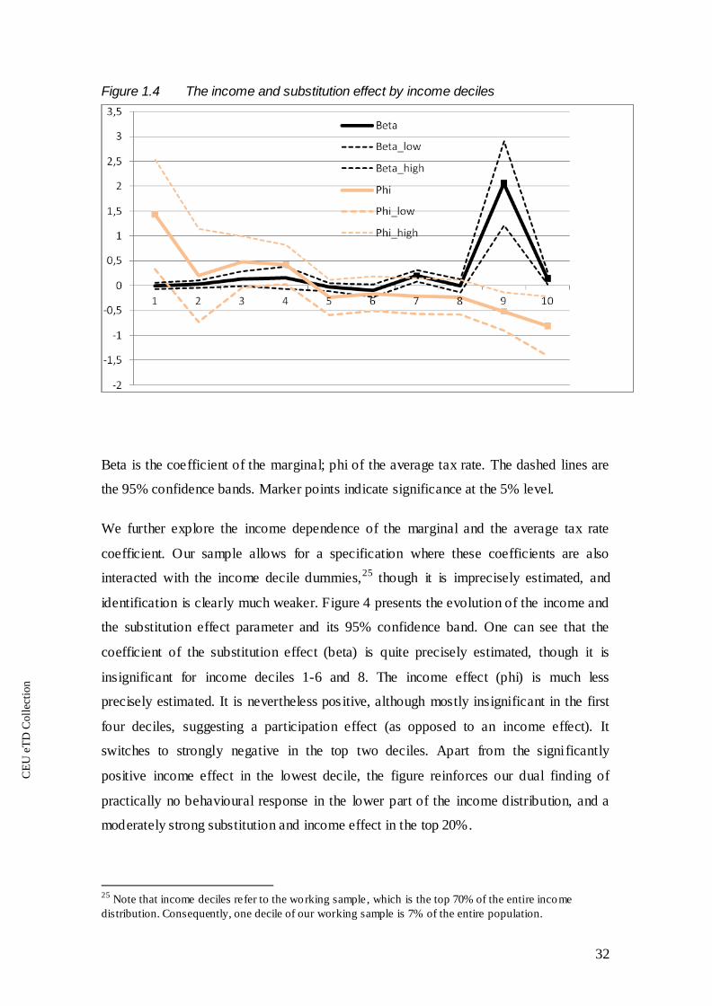
CE

UeT

DC

olle

ctio

n

32

Figure 1.4 The income and substitution effect by income deciles

Beta is the coefficient of the marginal; phi of the average tax rate. The dashed lines are

the 95% confidence bands. Marker points indicate significance at the 5% level.

We further explore the income dependence of the marginal and the average tax rate

coefficient. Our sample allows for a specification where these coefficients are also

interacted with the income decile dummies,25

25 Note that income deciles refer to the working sample, which is the top 70% of the entire income distribution. Consequently, one decile of our working sample is 7% of the entire population.

though it is imprecisely estimated, and

identification is clearly much weaker. Figure 4 presents the evolution of the income and

the substitution effect parameter and its 95% confidence band. One can see that the

coefficient of the substitution effect (beta) is quite precisely estimated, though it is

insignificant for income deciles 1-6 and 8. The income effect (phi) is much less

precisely estimated. It is nevertheless positive, although mostly insignificant in the first

four deciles, suggesting a participation effect (as opposed to an income effect). It

switches to strongly negative in the top two deciles. Apart from the significantly

positive income effect in the lowest decile, the figure reinforces our dual finding of

practically no behavioural response in the lower part of the income distribution, and a

moderately strong substitution and income effect in the top 20%.

CE

UeT

DC

olle

ctio

n

33

Finally, we check whether the elimina tion of those taxpayers who had po tential

problems with their reported employee tax credit numbers matter for the income and

substitution effect parameters. 26

Table 1.6. The inclusion of taxpayers with problems in their reported employee tax credit

As Table 1.6 suggests, the estimates change very little.

∆log taxable income Top 70% 70-20% Top 20%

without tax credit problems

with tax credit

problems

without tax credit problems

with tax credit

problems

without tax credit problems

with tax credit

problems ∆log (1 - marginal tax rate) 0.0648** 0.0562** 0.0292 0.0335* 0.337** 0.336** (0.016) (0.014) (0.015) (0.015) (0.059) (0.060) ∆log (1 - average tax rate) -0.0673 -0.0157 0.0443 0.104 -0.267* -0.244 (0.065) (0.066) (0.077) (0.078) (0.12) (0.13) First stage partial F For the marginal tax rate 2928.02 3558.43 3032.96 3261.54 317.52 317.34 For the average tax rate 2577.54 2616.30 1818.28 1879.84 745.33 726.78 Observations 146,676 150,141 104,857 108,247 41,819 41,894 Robust standard errors in parentheses. * significant at 5%; ** significant at 1% The p-values for the Kleibergen-Paap rk and the C-statistics are zero in all columns.

Summing up, we find lower elasticities for our larger sample than other empirical

studies. Concentrating on a medium-high income sample leads to an elasticity of around

0.3, already in the high range of the international evidence. As Gruber and Saez (2002)

indicate, high tax price elasticities for the U.S. are likely to be driven by itemizing,

which is a cost reduction status that can be chosen by all taxpayers. Employees are also

entitled to some cost deductions in Hungary, but their coverage and impact is very

limited. 27

26 Employee tax credit is calculated based on wage income capped by the monthly minimum wage times the number of elig ible months, and then it is phased out according to broad income. The ‘number of elig ible months’ variable is missing from our original dataset. We recovered this variable by allowing its value to go from 0 to 12 and selecting the one with which we get back the reported tax cred it (with a rounding error of 2.1, which allows for mult iple rounding errors before summing up). For around 5500 taxpayers, none of the values 0-12 were able to rep licate their reported tax credit. We attribute this to the fact that tax credit ru les are quite complicated and our data contains unaudited tax files. The difference never exceeds 12.25, which means that this problem is neglig ible for the average tax rate. The phase-out of the employee tax cred it, however, creates complicated patterns for the marg inal tax rate, which might be sensitive to such miscalculations. 27 In our sample, roughly 10% of all taxpayers report some cost deductions. These deductions usually refer to labor income derived from secondary income sources, where either a flat rate or an itemized deduction applies. The average deduction, however, is 163, compared to the average income of 3041 in this group.

This is likely to reduce tax price elasticity, as a major margin of adjustment is

CE

UeT

DC

olle

ctio

n

34

missing. Combining this observation with the fact that we had only a one year

difference between our pre- and post-reform observations, our elasticity results are

rather high.

Limiting the potential channels of adjustment

Here, we explore the importance of two adjustment mechanisms: first, we check the

heterogeneity of our results with respect to cost deduction status. Table 1.7 shows that

those who do not have cos t deductions show a higher substitution effect, but a zero

income effects. This suggests that the population-wide substitution effect in the top 20%

is largely unrelated to cost deductions, while the income effect might come from

deductions. Given the fact that deductions are, on average, 1% of taxable income in all

of our subsamples, the income effect coefficient of the deduction group may reflect their

higher overall flexibility in declaring income, and not deductions themselves.

CE

UeT

DC

olle

ctio

n

35

Table 1.7. Heterogeneity by cost deduction status

∆log taxable income Top 70% Top 20% 70-20%

No hete-

rogeneity Hetero- geneity

No hete-rogeneity

Hetero- geneity

No hete- rogeneity

Hetero- geneity

∆log (1 - marginal tax rate) Total 0.0648** 0.337** 0.0292

(0.0166) (0.0674) (0.0158)

No deduction 0.0608** 0.420** 0.0269

(0.0174) (0.0885) (0.0166)

Deduction 0.0777* 0.2041* 0.0405

(.0329) (0.0929) (0.0348)

Difference 0.0169 -0.216 0.0136

(0.0335) (0.119) (0.0363) ∆log (1 - average tax rate) Total -0.0673 -0.267* 0.0443

(0.0693) (0.146) (0.0786)

No deduction 0.0857 0.0518 0.127

(0.0751) (0.171) (0.0832)

Deduction -0.7173** -0.9409** -0.4426*

(0.1434) (0.2388) (0.1937)

Difference -0.803** -0.993** -0.570**

(0.154) (0.272) (0.205) Observations 146,676 146,676 41,819 41,819 104,857 104,857

Robust standard errors in parentheses. * significant at 5%; ** significant at 1% All specifications contain the cost deduction dummy as an extra control. The specification interacts realized and synthetic tax price variables with deduction status dummies. The p-values for the Kleibergen-Paap rk, the C- and the first stage partial F statistics are all zero.

Second, we look at heterogeneity with respect to being pure wage earners (Table 1.8).

Wage earners exhibit a higher (top 70%, top 70-20%) or an equal (top 20%) substitution

effect. The income effect is estimated very imprecisely, but again, there is no marked

difference between pure wage earners and those who have additional sources of income.

Overall, this finding suggests that shifting between capital and labour income has a

limited role in determining tax price elasticities. Given that pure wage earners have

limited room for income underreporting, it also weakens the case for tax avoidance as a

key determinant. This is in contrast to the finding of Gorodnichenko et al (2009) for

Russia.

CE

UeT

DC

olle

ctio

n

36

Table 1.8. Heterogeneity by “wage earner” status

∆log taxable income Top 70% Top 20% 70-20%

No hete-

rogeneity Hetero-geneity

No hete- rogeneity

Hetero-geneity

No hete-rogeneity

Hetero-geneity

∆log (1 - marginal tax rate) Total 0.0648** 0.337** 0.0292

(0.0166) (0.0674) (0.0158)

Wage earner 0.0761** 0.3337** .04209*

(0.0179) (0.0816) (0.0174)

Has nonwage income

0.0272 0.344** -0.0155

(0.0292) (0.0997) (0.0302)

Difference 0.0489 -0.0098 0.0576*

(0.0307) (0.120) (0.0329) ∆log (1 - average tax rate) Total -0.0673 -0.267 0.0443

(0.0693) (0.146) (0.0786)

Wage earner -0.0579 -0.2175 0.0688

(0.0804) (0.1755) (0.0915)

Has nonwage income

-0.0680 -0.331 0.0484

(0.109) (0.215) (0.130)

Difference 0.0101 0.113 0.0204

(0.126) (0.256) (0.152) Observations 146,676 146,676 41,819 41,819 104,857 104,857

Robust standard errors in parentheses. * significant at 5%; ** significant at 1% All specifications contain the wage earner status dummy as an extra control. The specification interacts realized and synthetic tax price variables with wage earner dummies. The p-values for the Kleibergen-Paap rk, the C- and the first stage partial F statistics are all zero.

1.5 Flat tax predictions

We now quantify the implications of a hypot hetical flat income tax proposal of a tax

rate of 30,3% above the 2005 minimum wage (684,000) and a 13,5% social security

contribution rate. These rates are applied to all components of taxable income. This

means that tax deductions are eliminated; and all incomes that used to be part of the tax

base but were previously untaxed (like scholarships) are now taxed the same way as any

other personal income item.

CE

UeT

DC

olle

ctio

n

37

The single tax rate is chosen in a way that the proposal is revenue neutral in case of no

behavioural response. 28 Eliminating the tax exempt status of the minimum wage would

imply a combined rate of 32%. This is close to CEE flat tax rates, but those flat tax

schemes also involve a tax-exempt income range. Consequently, our 13.5+30.3% rate is

high compared to other flat tax rates in the CEE region. 29

Let us stress that this reform does not change the overall tax rate below the minimum

wage. Our reasons are twofold: on the one hand, we do not have reliable estimates for

taxpayer behaviour below the minimum wage; on the other, an increase in the marginal

and the average tax rate for this income group is likely to involve substantial social

tensions.

It is also somewhat higher

than the current flat rate proposal in Hungary (a combined rate of approximately 33%,

no zero rate).

30

We apply this tax scheme to 2005 income data under three scenarios. Scenario 1

assumes no behavioural effect at all. Scenario 2 assumes no income effects and the

appropriate substitution effect (an elasticity of 0.0291 in the top 70-20 % and 0.336 in

the top 20%). Scenario 3 works with the same substitution effect and adds the income

effect (a parameter of -0.271) in the top 20%.

31

As this tax scheme still makes the marginal and average tax rate endogenous, we predict

income changes the following way. First we calculate the ‘no behavioural response’

case by inserting original 2005 incomes into the new tax scheme. Then we calculate the

change in income implied by the realized marginal and average tax rates corresponding

to scenario one. This new income leads to different realized tax rates, with which we

Although such a large tax change may

induce larger behavioural responses, the literature does not point to a particularly

important nonlinearity.

28 A 41.3% combined rate would be revenue neutral under our baseline behavioral response scenario. 29 Ivanova et al (2005) g ives an international comparison: flat tax personal income tax rates range from 12% to 19%. Based on more recent and more comprehensive comparisons (Keen et al, 2006 and www.worldwide-tax.com), th is range is between 10% and 25%. Ivanova et al (2005) also report that there was an additional social security contribution rate and a tax-exempt ‘zero b racket’ in Russia, while Moore (2005) indicates the same fo r Slovakia. 30 Actual flat tax schemes are often similar. For example, the flat tax scheme in Slovakia involves a single rate above some tax-exempt threshold, and social security contributions are kept separately. 31 According to our detailed estimates, the substitution and income effects are much less precisely known for the top of the income distribution. A flat tax, however, has a very similar effect ont he marginal and the average tax rate of top earners. It means that as long as the uncompensated elasticity is small, the reaction of top earners is not pivotal for our predict ions. Setting both the substitution and the income effect to zero in the top 2% (see Table 1.9) slightly increases our predicted revenue and income gains.

CE

UeT

DC

olle

ctio

n

38

upda te our income estimate. This iterative process leads to a solut ion where our

predicted post-reform incomes are consistent with the appropriate realized tax rates. 32

Figure 1.5 Average and marginal tax rates: before and after the flat income tax scheme

Figure 1.5 depicts the change in the average and marginal tax rates (the former is

calculated under Scenario 3) as a function of pre-reform 2005 income (in a 2% random

sample for better visibility). It is immediately visible that there is a substantial increase

in the average tax rate between the minimum wage and 2,000,000; and most of the fall

in the marginal tax rate concentrates in the range 2,000,000-6,000,000. We will return to

the former property in the incidence analys is; the latter, however, is quite desirable,

since taxable income is quite sensitive to the tax price in that income range.

.1.2

.3.4

.5

0 2000 4000 6000 8000 10000original income

average tax rate post-reform ATR

Panel A: average tax rates

.2.4

.6.8

mar

gina

l tax

rate

0 2000 4000 6000 8000 10000original income

pre-reform MTR post-reform MTR

Panel B: marginal tax rates

32 In practice, this procedure is much simpler. Without an income effect, there is only one necessary adjustment: those who start above 684,000 but would go below as a response to higher marginal tax rates bunch at exactly 684,000. Anyone who remains above the minimum wage will be subject to a marginal tax rate of 43.8%. For the income effect, we first use the ‘no behavioral response’ ATR (calculated in Scenario 1). Th is leads to some income change, which then implies a slightly different realized ATR. In the next step, we modify our predicted income change by the log difference of these two (one minus) ATRs, multip lied by the income effect coefficient. Then we calculate the corresponding ATR again and repeat the previous step till convergence. After the second step, the change becomes negligible.

CE

UeT

DC

olle

ctio

n

39

There is also a decline in marginal tax rates below the minimum wage. This is due to

the fact that our hypothetical tax scheme determines tax obligations based solely on

taxable income, while the original 2005 tax scheme often used broad income to

determine the tax payment on taxable income. As a matter of fact, most taxpayers

earning below the 2005 minimum wage would experience no change in their marginal

tax rate (34,436 out of 49,647).

Table 1.9 summarizes the main implications of our flat income tax. According to the

design of our hypothetical reform, without a behavioural response there is no change in

budget revenues and taxable income. Adding the substitution effect leads to a 2.77%

increase in revenues, together with a 1.88% increase in after-tax income. These numbers

become somewhat smaller as we add the income effect: a 2.06% increase in revenues

and a 1.39% increase in after-tax income. If one gives up the revenue gain, the 30.3%

tax rate can be reduced to 27.9%. That would imply a 2.1% increase in pre-tax income

and a 3.9% increase in after-tax income. 33 These effects are substantial – total pretax

income is approximately one third of total GDP in Hungary, which is the base of the

32% employer contributions, and the approximately 32% income tax and employee

contribution -- but we do not see such a “miracle” as flat tax proponents would like. 34

33 Under the 41.3% combined tax rate scenario, the inclusion of the substitution and the income effect leads to zero revenue gain, and an increase of 2.1% of p retax income and a 4.04% increase in aftertax income. 34 Apart from addit ional effects through the extensive margin, the increase in total pretax income is an upper bound on the shift of labor supply. In case of a constant returns to scale technology, this also limits the general equilibrium impact on total production (GDP). If the rate of return on capital is unchanged, then labor demand is flat and the shift in labor supply equals the increase in output. If the rental rate has to increase to absorb the extra supply of labor, then output increases by less than the shift in labor supply.

CE

UeT

DC

olle

ctio

n

40

Table 1.9. Implications of a flat income tax scheme

Behavioural effects considered

None only subst. subst. and income

Percentage change in total Budget revenue (employee part only) 0.04 3.31 2.45 Budget revenue (employee and employer) 0.02 2.77 2.06 pretax income 0 2.30 1.71 after-tax income -0.02 1.88 1.39 Pretax income, % change in p90/p10 0 5.08 4.18 p90/p50 0 5.64 4.74 p10/p50 0 0.56 0.56 p75/p25 0 2.16 2.16 p75/p50 0 2.17 2.17 p25/p50 0 0.00 0.00 Gini (pre reform: 0.46023) 0.46023 0.46038 0.4655 After-tax income, % change in p90/p10 0.07 4.62 3.81 p90/p50 11.48 17.03 16.10 p10/p50 11.23 11.78 11.78 p75/p25 -2.40 -0.54 -0.54 p75/p50 5.90 7.73 7.73 p25/p50 8.55 8.25 8.25 Gini (pre reform: 0.38529) 0.39582 0.403536 0.40116

For a full description of the three scenarios, see the main text. Variables like p90/p10 refer to the ratio of the 90 and 10 percentile of the income distribution.

There are, however, notable changes in the income distribution (due to the nature of our

data, we are talking about the distribution of taxpayer individual and not household

income). In pretax income, the most substantial change is in the 90-10 percentile (p90-

p10) and the p90-p50 ratio, an increase of 4-5.5%. In after-tax income, there are similar

changes in the p90 -p10 ratio, but all ratios involving the median are much higher. This

is in line with our observation that there is a substantial increase in the average tax rate

between the minimum wage and 2,000,000 (see Figure 1.5). The Gini coefficient of

pretax income increases from 0.46023 to 0.4655; while for after-tax income, it increases

from 0.38529 to 0.40116. 35

35 These changes in the Gini coefficient are roughly similar to typical annual changes in the Gini coefficients of per household member income, indiv idual income and individual labor income. Most percentile rat ios, on the other hand (like p90/p10) change much more during our hypothetical reform than

This increase is partly driven by the change in tax rates, and

CE

UeT

DC

olle

ctio

n

41

partly by the behavioural response: without the latter, the after-tax Gini would be

0.39582.

Figure 1.6 The percentage change in after-tax income by 2005 after-tax income deciles

-10

-8

-6

-4

-2

0

2

4

6

8

10

1 2 3 4 5 6 7 8 9 10

No behavioral response Only subst. effect Subst. and income effect

To illustrate the detailed incidence of the tax reform36

in a typical year (Kapitány and Molnár, 2005). Note that our calculations cannot take into account individuals without taxable income and red istribution within households. Consequently, these Gin i numbers cannot be directly compared to typical measures of income inequality across households. Still, as Benedek and Lelkes (2006) suggests, the distribution of household income and individual income are quite similar. 36 Benedek and Lelkes (2006) discuss the redistributional aspects of a flat tax reform at depth.

and the impact of behavioural

responses, Figure 1.6 plots the percentage change in the average after-tax income for

pre-reform after-tax income deciles, for Scenarios 1, 2 and 3. There is a substantial

increase in the average income level in the first two deciles and some increase in the

third decile, which are unaffected by the presence of behavioural responses. There is a

small decline in decile 4, and a very sizable fall in deciles 5-7. In deciles 4-6, the

behavioural response works against taxpayers as they experience a small increase in

their marginal tax rates as well. In decile 7, the behavioural response alleviates the

impact of higher average tax rates; in decile 8, it turns an income loss into an income

gain. Finally, deciles 9 and 10 experience a sizable increase in their income. The

behavioural response is most notable in decile 9, increasing the gain from 1.23% to

5.25%.

CE

UeT

DC

olle

ctio

n

42

In summary, these three cases illustrate the importance of the elasticity of taxable

income to changes in the marginal tax rate. Even the internationally small elasticity

estimate (0.0648) has a remarkable effect on the government’s budget, while the 0.337

elasticity is very influential for tax revenue developments. Based on our flat tax results,

there is room for a parallel improvement of budget revenues and taxable income. Such a

reform, however, involves important changes in income inequality, and its burden falls

mostly on lower-middle income taxpayers.

Let us also stress the importance of the income effect. Table 1.9 and Figure 1.6 show

that its presence has very important quantitative effects on income and revenue

predictions. In particular, a reduction in the average tax rate of top earners leads to a

substantial decrease in their income gain brought about by lower marginal tax rates (see

income decile 10 on Figure 1.6).

A comment is in order regarding the current Hungarian flat tax po licy debate. A special

feature of Hungarian personal income taxation is the system of employee tax credits,

which makes low (wage) incomes untaxed, at the expense of higher marginal tax rates

in a phase-out range. Our finding of a low substitution effect below the top 20% of the

income distribution and a substantial substitution effect above it implies that the

location of the phase-out range is quite important. If it falls heavily in the top 20%

bracket, the high marginal tax rates can deter income generation due to the substitution

effect. According to the 2010 tax system, the phase-out range goes well into the top

20% bracket. Consequently, a flat tax proposal that would eliminate such an employee

tax credit scheme (or at least lower the phase-out range) can generate more substantial

gains than our predictions would suggest. According to preliminary calculations of

Scharle et al (2010), the sheer reduction of the phase-out range below the top 20% range

can generate budget revenues of around 1% of GDP.

CE

UeT

DC

olle

ctio

n

43

1.6 Conclusions

In evaluating tax policies and forecasting the effects of future tax changes, it is essential

to distinguish the influence of changing tax rates and changing law enforcement. In case

of extensive tax reforms it is usually not possible. Hungary introduced a medium-scale

reform in 2004/2005 without any changes in tax audit rules and practices. We used this

occasion to analyze the behavioural response of taxable income to marginal and average

tax rates.

Our empirical analysis suggests an overall tax price elasticity of about 0.06 in Hungary.

Though this number is significantly lower than elasticities found in other countries,

even this low elasticity can have some effect on the government’s budget. Moreover,

the upper 20% of the population exhibits a much higher elasticity, exceeding 0.3, and

even as high as 0.45 for some income groups. This is already at the high end of the

international evidence. We demonstrated that such elasticities have important impacts

on the income generation process and budget revenues.

These results are mixed news for flat tax proponents: the low overall elasticity indicates

that cutting marginal tax rates might not lead to such an economic stimulus as many

would expect. For the upper 20% of the population, however, a decrease in marginal tax

rates may indeed lead to a substantial increase in income generation, which would also

exacerbate the adverse redistributional aspects of such a reform.

Our detailed flat income tax simulation confirmed these general points. In particular, we

calculated the impact of a reform that keeps the existing 13.5% combined income tax

and social security contribution rate below the annua l minimum wage, and its single

rate above the minimum wage is selected in such a way that there is no effect on budget

revenues in case of no behavioural respons. This revenue neutral flat tax rate (30.3%

income tax plus 13.5% social security) is high compared to other flat tax rates in the

CEE region.

We predict a roughly 2% improvement of budget revenues and a 1.4% increase in

taxable income, which is significant but rather modest. On the other hand, there are

important changes in the income distribution, and the overall burden falls mostly on

lower-middle income taxpayers (income deciles 5-7).

CE

UeT

DC

olle

ctio

n

44

Besides the flat tax predictions, our results have a number of additional, potentially

important, policy implications. One is that the conclusions of Gruber and Saez (2002)

for the US also apply to Hungary – both in terms of the desirability of low marginal

taxes on a broad income basis, and in terms of the potentially low distortion caused by

the high marginal tax rates of phasing out employee tax credits.

The first statement is supported by our highly positive marginal tax price elasticity

estimate. As compared to the US, where much of the elasticity is likely to be due to

itemized deductions, we find that deductions do not contribute to the sensitivity of

taxable income to marginal tax rates. Combined with the finding that wage earners

exhibit similar estimates of the substitution effect, it suggests that the elasticity we find

may be much closer to a true “generalized” labour supp ly elasticity than the US

findings.

The second claim is based on the finding that the same elasticity is much lower in the

income range 636,000-2,000,000 where employee tax credits are phased out (in 2004

and 2005). On the other hand, the marginal tax rates implied by phasing out other tax

allowances are likely to cause substantial losses, as those extra 10-20% marginal rates

apply to taxpayers with substantial tax price elasticity and high preexisting marginal tax

rates. This also applies to the 2010 phase-out range of employee tax credits.

CE

UeT

DC

olle

ctio

n

45

Bibliography

Income Tax Act CXVII, 1995.

Aarbu, K. O., and T. O. Thoresen (2001). "Income Responses to Tax Changes -

Evidence from the Norwegian Tax Reform." National Tax Journal, 54(2): 319-338.

Auten, G. and R. Carroll (1999). "The Effect of Income Taxes on Household Income."

The Review of Economics and Statistics, 81(4): 681-693.

Baum, C. F., M. E. Schaffer, and S. Stillman (2007). “Enhanced routines for

instrumental variables/GMM estimation and testing.” Boston College, Department of

Economics, Working Paper No. 667.

Benedek, D. and O. Lelkes (2006). “An examination of income redistribution in

Hungary and single-rate tax reform, using a micro-simulation model.” Közgazdasági

Szemle, LIII(7): 551-572. (in Hungarian)

Blomquist, S. and H. Selin (2010). “Hourly wage rate and taxable labor income

responsiveness to changes in marginal tax rates.” Journal of Public Economics, 94

(2010): 878–889

Chetty, R. (2008). “Is the taxable income elasticity sufficient to calculate deadweight

loss? The implications of evasion and avoidance.” NBER Working Paper

2008/13844

Eissa, N ., H. Jacobsen Kleven and C. T. Kreiner (2004). „Evaluation of four tax reforms

in the United States: Labor supply and welfare effects for single mothers.” NBER

Working Paper 2004/ 10935.

Eppich, Gy. and Sz. Lőrincz (2007). ”Three methods to estimate the whitening-related

distortion of the wage statistics.” MNB Studies. 2007/66.

Feldstein, M. (1995). "The Effect of Marginal Tax Rates on Taxable Income: A Panel

Study of the 1986 Tax Reform Act." Journal of Political Economy, 103(3), 551-572.

Feldstein, M. (2002). "The Transformation of Public Economics Research: 1970-2000,"

Journal of Public Economics, 86(3), 319-326.

Gorodnichenko, Y., J. Martinez-Vazquez and K. Sabirianova Peter (2009). “Myth and

Reality of Flat Tax Reform: Micro Estimates of Tax Evasion Response and Welfare

Effects in Russia.” Journal of Political Economy, 117 (3), 504-554.

Gruber, J. and E.Saez (2002). "The Elasticity of Taxable Income: Evidence and

Implications." Journal of Public Economics, 84 (1), 1-32.

CE

UeT

DC

olle

ctio

n

46

Heckman, J. (1993). "What Has Been Learned About Labor Supp ly in the Past Twenty

Years?" American Economic Review, 83(2), 116-121.

Ivanova, A., M. Keen and A. Klemm (2005). ”The Russian flat tax reform.” Economic

Policy, 20(3), 397-444.

Kapitány, Zs. and Gy. Molnár (2005). “The mobility of household income and

consumption in Hungary around 2000.” In: Households on the market for knowledge

and labor (eds. Kapitány, Zs., Molnár, Gy. and Virág, I.) IE-HAS Books. Institute of

Economics, Hungarian Academy of Sciences, Budapest.

Keen, M., Y. Kim and R. Varsano (2006). “The ’Flat Tax(es)’: Principles and

Evidence.” IMF Working Paper, 2006/218.

Kiss, Á. (2010): “The Elasticity of Reported Income of Top Earners.” Discussion Paper,

Office of the Fiscal Council of Hungary (in Hungarian)

Krekó, J. and G. P. Kiss (2007). "From Tax Optimization to Optimal Taxation - The

First Step: Tax Compliance and the Hungarian Tax System." MNB Studies, 2007/65.

Lindsey, L. B (1987). "Individual Taxpayer Response to Tax Cuts: 1982-1984." Journal

of Public Economics 33(2) 173-206.

Ljunge, M. and K. Ragan (2005). “Labor Supply and the Tax Reform of the Century”,

Working Paper, Department of Economics, University of Chigaco, August 2005.

Moffitt, R. A., and M. Wilhelm (2000). "Taxation and the Labor Supp ly Decision of the

Affluent." In: Does Atlas Shrug? The Economic Consequences of Taxing the Rich.

(ed. Slemrod, J.), Cambridge University Press, Cambridge.

Moore, D. (2005). “Slovakia’s 2004 tax and welfare reform.” IMF Working Paper,

2005/133.

Mosberger, P. (2010). “Taxable Income Elasticity Estimation of Top Earners in

Hungary.” Master’s thesis, Central European University

OECD (2005). Taxing Wages. Paris: OECD Publications.

OECD (2004). Taxing Wages. Paris: OECD Publications.

Papp, T. and E. Takats (2008). “Tax rate cuts and tax compliance – the Laffer curve

revisited.” IMF Working Paper 2008/7.

Saez, E., J. Slemrod and S. Giert (2010). "The Elasticity of Taxable Income with

Respect to Marginal Tax Rates: A Critical Review" Journal of Economic Literature,

forthcoming

Scharle, Á. (2005). "The Effect of Tax- and Social Benefit System on the Labor Supply:

What does the Marginal Effective Tax Rate Show?" In European Employment

CE

UeT

DC

olle

ctio

n

47

Strategy: Opportunities and Barriers for the New Member States, (ed. Á Hárs, E

Landau and K Nagy). Budapest. Kopint-Datorg.

Scharle, Á., P. Benczúr, G. Kátay and B. Váradi (2010). “How Can We Increase the

Efficiency of the Hungarian Tax System?” Working Papers in Public Finance, 26 (in

Hungarian)

Semjén, A. and I. J. Tóth (2004). “The hidde n economy and taxation-related behaviour,

1996-2001.“ Közgazdasági Szemle, LI. (6): 560-583. (in Hungarian) An English

version is available at: http://www.wargo.hu/tij/kutatas/tax/ado021e.pdf

Sillamaa, M. and M. R. Veall (2001). "The Effect of Marginal Tax Rates on Taxable

Income: A Panel Study of the 1988 Tax Flattening in Canada." Journal of Public

Economics, 80(3): 341-356.

Vidor, A. (2005). “The effect of saving incentives: Empirical evidence from Hungary.”

Working Papers in Public Finance 2005/15.

CE

UeT

DC

olle

ctio

n

48

Appendix

A. Changes in the Hungarian tax system, 2004-2005

The four key elements of the 2004-2005 tax reform were the following (Income Tax Act

1995; OECD, 2004 and 2005).

Reduction of the number of tax brackets from three to two. Taxpayers with taxable

income between 800,000 and 1,500,000 experienced an 8 percentage point decrease in

their marginal tax rate. The tax schedule in Table A1.a changed to the schedule in Table

A1.b.

Table A1.a Tax schedule in 2004

Number of tax filers 0 – 800 000 18 % 1 815 111 800 001 – 1 500 000 26 % 1 138 156 1 500 001 - 38 % 1 196 610

Source: http://www.apeh.hu/adotablak and Tax and Financial Control Office

Table A1.b Tax schedule in 2005

Number of tax filers 0 – 1 500 000 18 % 2 806 935 1 500 001 - 38 % 1 342 948

Source: http://www.apeh.hu/adotablak and Tax and Financial Control Office

The maximum amount of the supplementary employee tax credit was increased from

540 per month to 1260 per month. The phase out interval for the supplementary tax

credit was changed from 720,000-756,000 to 1,000,000-1,302,000, which also means

the changing of the phase out rate from 18% to 5%. 37

37 In Hungary the employee (earned income) tax credit has two parts, the main ‘tax cred it’ and the ‘supplementary tax cred it’. Both are applicable after earned wage income, therefore entrepreneurs are excluded from these allowances. The two together guaranteed the tax exempt status of the min imum wage until 2006. Both have a gradual phase out, although the two intervals differ.

CE

UeT

DC

olle

ctio

n

49

An income limit was introduced both for the family tax allowance and for the sum of

other tax allowances. Parents are eligible for the total amount of the family tax

allowance if their broad income is below 8,000,000, above this limit the allowance is

phased out by a rate of 20%. 38

B. The identification scheme

Broad income consists of wage income, non-wage labor

income (the sum of these two is our taxable income measure), and other, mostly capital

incomes (taxed separately). For the sum of other tax allowances the maximum amount

of the allowance is 100,000 and the eligibility broad income limit is 6,000,000, above

which it is gradually withdrew (also at a rate of 20%).

The maximum of annual pension contribution was increased from 451,095 to 510,051.

This implies that the maximum income for pension contribution was changed from

5,307,000 to 6,000,600.

There were no changes in the rate of the social security contributions, namely in the

pension, sickness and the unemployment scheme, their level remained 8.5, 4 and 1

percent respectively.

Following Gruber and Saez (2002), we write the change in income as a sum of the

subs titution and the income effect:

( ) 1d .

1 1y d dR yd u

y yτ τβ φτ τ

−= − + +

− − (4)

Here the first regressor is the realized change in ln(1-mtr), while the second is the

realized c hange in ln(1-atr). For this latter step, one needs an extra assumption: y(1-τ) ≈

y-yτ +R. This is also adopted by Gruber and Saez (2002). This is then how the

approximation works:

( )

( ) ( ) .11

loglog

1

ττ

τττ

ττττ

−−

=−−

−−+≈

−−+

−−+=

−+=

−

−

yyddR

ydy

yyddydydR

ydy

yyRyddydydR

yyyRd

yyTyd

ATR

38 Family tax allowances, just like other elements of the income tax system, work on an individual basis, i.e. parents can decide which of them requests the tax allowance, and they also have the option to split the amount.

CE

UeT

DC

olle

ctio

n

50

Notice that Gruber and Saez (2002) do no deduct the dy/y term. That distorts the

parameters – their estimates need to be divided by 1-φ, which is essentially one for

them, finding no income effects. For us it does matter as our φ is often nonzero.

Equation (4) cannot be estimated via OLS because the realized tax rate changed for two

reasons: tax reform (exogenous variation) and income dependence of the tax scheme

(endogenous variation). The proposed solution is to instrument each tax rate variable by

its “synthetic” version, which is the change in the appropriate tax rate implied by the

change in legislation, applied to unchanged real income.

Formally, this is how identification works. Assume that

( ) ( ), and , ,y R R yτ τ λ λ= =

where λ is a parameter indexing the tax reform. Using a first order approximation:

( )

1 2

1 2

1

.1

d dy dy

dR yd dyR R dy y

τ τ τ λττ λ

τ

= +−

−= +

−

Here in principle the second term is nothing but the change in the synthetic tax rate: the

change in ln(1-mtr) implied by reform λ, for an unchanged income level. As any

practical reform is a discrete change, the first order approximation is surely not precise

– meaning that there is a separate error term corresponding to this equation, moreover,

the coefficient of the synthetic tax rate change can differ from one. 39

( )

1 2 2

1 2 3

1

.1

d dy ms uy

dR yd dyR R as uy y

τ τ τττ

τ

= + +−

−= + +

−

Thus we write the

equations for the realized tax rate changes as follows:

Here the variable ms is the shorthand for the change in the synt hetic (unchanged real

income) log one minus marginal tax rate, and as is the same for the average tax rate.

Based on this, it is straightforward to see that the original regression (4) is misspecified

– both of the right hand side terms contain the error term u1 in general (unless there is

no endogeneity problem in the sense that the tax rate – be it the marginal or the average

39 Running exp loratory regressions confirms this: regressing the realized MTR change on all controls plus

the change in income and the synthetic MTR change, with income change instrumented by the synthetic

change in ATR yields a synthetic MTR coefficient around 0.3. The same argument applies to the ATR

equation: here we get a coefficient of 0.9, still differing from one at the 5% level.

CE

UeT

DC

olle

ctio

n

51

– does not change with income levels).

Equation (4) can still be estimated by single equation IV. We run (4) by using ms and as

as instruments – they are uncorrelated with the error terms and (by the reduced form)

are correlated with the realized tax rate changes. This identifies β and φ.

CE

UeT

DC

olle

ctio

n

Chapter 2

Entrepreneurial Tax Changes in Hungary: Tax price Elasticity of the Self-employed

2.1 Introduction

In the first chapter of this thesis I showed that employees in Hungary react to tax

changes substantially. In this chapter I investigate the elasticity of reported income of

the self-employed to tax rate changes and decompose it to labour supply response and

other factors, more importantly tax evasion. Taxable income can change for several

reasons besides changes in labour supp ly. As a response to tax changes, individuals

might increase their work effort and tax-deductible activities, renegotiate their

compensation package includ ing non-cash elements and can also change their income

underreporting behaviour. 1

In the last few decades an extensive body of literature has emerged on the elasticity of

taxable income to changes in the marginal tax rate. Most studies find a significant

positive effect of decreasing tax rates on reported income. Some of these studies also

suggest that only part of this response comes from increased labour supply, while

taxpayers also adapt to changes by altering the form of compensation and tax evasion.

The substitution of unreported income by reported income as a response to tax rate

changes might increase with the income underreporting possibilities, e.g. in case of

Usually, these components are very difficult to separate

(Gorodnichenko et al, 2009 is one of the few exceptions that separates the labour supply

and tax evasion responses). Entrepreneurs are self-employed, therefore the role of in-

kind benefits is probably very low, and hence the two major elements defining the

taxable income response are the labour supp ly and the tax evasion effects.

1 For the self-employed there are possible other margins of adjustment too, e.g. timing of income flows or attributing parts of the self-employment income to other family members, but these effects cannot be estimated based on the individual tax report data.

CE

UeT

DC

olle

ctio

n

53

small enterprises or in economies with extensive black economies. Several authors2

found that tax evasion was more widespread among entrepreneurs than employees. In

spite of this finding, only a few studies estimate the tax responsiveness of the self-

employed 3

The aim of this chapter is to analyse elasticity of reported income of self-employed to

tax changes in Hungary and to isolate the true labour supp ly elasticity of entrepreneurs.

To guide this empirical analysis, I develop a simple model of the behaviour of the self-

employed that takes into account both labour supp ly and tax evasion. The basis of the

model is the usual deterrence model, where the expected utility is determined by the

probability and penalty of tax evasion. First, I present a simple form of the model

showing how labour supp ly response can be separated from tax evasion effects. Then I

add the special tax rules applying to the self-employed. I test this model empirically on

individual tax returns data and demonstrate that at least part of the income response to

tax rate changes comes from tax-avoidance and not from increased income-generating

efforts.

.

In this chapter, I argue that overall elasticity of the self-employed is 7-12%, and

elasticity reduces to about half when controlled for tax evasion. Therefore, the true

labour supp ly elasticity of the self-employed is around 5%. For the estimation I use a

Hungarian tax reform episode. Hungary introduced a new type of tax, called “Simplified

Entrepreneurial Tax” (EVA) as of January 2003, under which there is a substantially

lower tax rate and simplified tax administration. The tax base is different from the

general case, it is based on the gross income of the enterprise instead of the usual net-of-

VAT revenue. This also means that EVA taxpayers do not report costs of operation.

The overall elasticity is lower than comparable European estimates for employees, but

almost twice as large as the overall elasticity of employees in Hungary. An explanation

for low elasticity is that most of the self-employed minimise their tax payment by tax

evasion and tax avoidance under all conditions; therefore, they are not very respons ive

to tax rate changes. However, estimated labour supply elasticity is fairly modest, so

self-employed individuals to some extent do react to tax rate changes in their real labour

efforts.

2 For example the stream of literature apply ing the consumption-based estimation of tax evasion following Pissarides and Weber (1989). 3 See Kopczuk (2010) on Po lish data for example.

CE

UeT

DC

olle

ctio

n

54

The chapter is organised as follows. Section 2 reviews the relevant empirical literature;

section 3 describes the methodology of the analysis, including the description of the

dataset; section 4 presents main results of the analysis; and section 5 concludes.

2.2 Related literature

The first stream of empirical studies on labour income taxation dealt with labour supply

elasticity estimations (Heckman, 1993 gives a summary of these studies). In these

studies labour supply participation is found to be more elastic to tax rate changes than

labour supp ly on the intensive margin, measured by the hours worked, and also

secondary earners (usually women) are found to be more elastic on both margins than

pr imary earners4

Estimates on elasticity range from very low (even negative e.g. Aarbu and Thoresen,

2001) up to some very high (close to 1, e.g. Feldstein, 1995) figures. Typically, US

taxpayers are somewhat more elastic than Europeans (Gruber and Saez, 2002 and Saez

et al, 2010 give a summary of the earlier results), and taxpayers with higher income

tend to react to a greater extent. However, as Gruber and Saez (2002) emphasise, tax

elasticity literature focuses on taxable income which contains labour supply responses,

adjustments in the form of compensation, unmeasured effort and tax compliance. These

. A more recent stream of literature focuses on the elasticity of taxable

income rather than labour supp ly. T he two streams of literature have different foci.

Labour supply is a real economic measure that has considerable influence on the output

of the economy. Therefore, it is a major policy concern is most countries, especially in

Europe, where ageing of the population results in high inactivity. Taxable income,

however, is a very important measure from a budgetary po int of view and captures

changes in the form of compensation and tax compliance as well. Most of these papers

concentrate on the elasticity of taxable income with respect to the change in the tax

price (net-of-tax income per marginal pretax dollar, i.e., one minus the marginal tax

rate). Usually the effect of tax changes on work efforts, and tax evasion are not

separated, but only changes in declared taxable income are considered. The estimated

elasticity varies subs tantially by the period and country examined and the regression

specification.

4 see for example Evers et al (2006).

CE

UeT

DC

olle

ctio

n

55

factors might even be more elastic to taxation than labour supp ly. In their work of

summarising labour supply literature, Blundell and MaCurdy (1999) state that male

labour supp ly elasticity to after-tax wages is low. However, they find that labour supp ly

responsiveness of secondary earners (generally women) can be much higher.

Starting from Feldstein (1995), applied empirical strategy to estimate the effect of tax

price on taxpayers’ income is very similar (in logs):

log(1 )it i t t i it ity c x MTR uγ α β= + + + − + (1)

where ity is taxable income, MTRit is the marginal tax rate, ic is the fixed effect for

individual i and tγ is a time-specific effect. The variables in ix are individual

characteristics that do not vary over time, but may have a time-varying effect on ity .

Finally, β is the elasticity of taxable income.

In the early studies income and substitution effects are not distinguished. Gruber and

Saez (2002) is the first study to distinguish these two effects of the tax changes. In their

study they include bot h the marginal tax rate and the virtual income or average tax rate

as explanatory variables for changes in the taxable income and also include controls for

the income mean reversion and changes in the income distribution. The overall

estimated elasticity of taxable income in Gruber and Saez (2002) is around 0.4 mostly

coming from the high elasticity of the high income taxpayers. However the income

effect is found to be insignificant.

Allingham and Sandmo (1972) make a seminal contribution to the tax evasion literature

with the deterrence model. In their mode l taxpayer is modelled as a gambler who

chooses reported income in order to maximize expected utility. Undeclared taxable

income has a payoff t, the rate of income tax with probability (1-p) and a penalty with

probability p. The expected payoff is (1-p)t-p. If it is positive, the taxpayer will evade.

Yitzhaki (1974) emphasised that it is important to distinguish if the penalty is imposed

on the income or the tax understatement.

All the early models of tax evasion considered only income understatement and

exogenous detection probability. F irst, Cremer and Gahvari (1994) set up a model of tax

evasion with a concealment technology where tax-evaders can influence their

probability of being caught. When audited, the probability of detection depends on the

CE

UeT

DC

olle

ctio

n

56

amount spent on concealment. They show that tax evasion in this form changes the

progressivity of the tax system.

Although it is very difficult to obtain reliable data on tax evasion, there is, however, a

subs tantial empirical literature on the topic. Most of the studies use the TCMP data,

which contains the result of successful tax audits in the United States. Slemrod and

Yitzhaki (2000) summarise tax evasion based on this dataset as follows. Based on the

audit coverage of around 1%, the estimated evasion is about 17% of the true tax

liability. Evasion greatly differs between social groups; for example, voluntary

reporting was 99.5% for wages and salaries whereas only 41.4% for self-employed.

Gorodnichenko et al (2009) in their recent empirical study separated tax evasion and

labour supp ly effect of a tax reform using Russian data. They follow the technique of

Pissarides and Weber’s (1989) to evaluate the 2001 Russian flat tax reform that brought

about a substantial tax cut: they use the difference be tween repo rted consumption and

income in the household budget survey to estimate tax evasion. Their major finding is

that tax evasion response to the tax cut was large, whereas the productivity response

was fairly modest as opposed to previous estimations. Therefore, the estimated welfare

gains of the reform are about 30% lower than other estimation approaches suggest. This

highlight s the fact that separating the tax evasion and productivity responses to tax cuts

might be necessary to evaluate tax reforms correctly.

The first chapter of this thesis (also as Bakos, Benczur and Benedek, 2009) estimated

tax price elasticity using Hungarian data following the method of Gruber and Saez

(2002) and found an elasticity of 6-30%. This estimation only covered the employed

population and excluded the self-employed.

From Elek et al (2009), we know that the self-employed on average declare a lower

income than the employed. Based on the dataset of the Central Administration of the

Hungarian Pension Insurance, Elek et al (2009) conclude that most entrepreneurs

declare a wage income around the minimum wage. Kreko and P. Kiss (2007) showed

that entrepreneurs tend to declare labour income as capital income in order to decrease

their tax obligations. Based on the comparison of administrative and survey datasets in

the third chapter of this thesis (also as Benedek and Lelkes, 2009) I argue that income

underreporting is higher among the self-employed than employees in Hungary.

CE

UeT

DC

olle

ctio

n

57

The above listed find ings emphasise the fact that tax evasion responses have subs tantial

revenue effect, probably even more so for the self-employed than for employees. To

understand the nature of this relationship, it is necessary to evaluate the tax evading

behaviour of small enterprises.

2.3 Empirical analysis

In this chapter of the thesis, I analyse the responsiveness of the self-employed to tax

changes in Hungary. To better understand the tax reporting behaviour, I use a deterrence

model, based on Allingham and Sandmo (1972), similar to the one applied by Tonin

(2009).

The self-employed choose their labour supply, true net cost of production and share of

hidden income. Their net income is defined by corporate tax, dividend tax, personal

income tax and social security contribution. Since taxes on wage income (PIT + ssc) are

greater than taxes on corporate income at all levels, they keep the level of wages at the

legal minimum, thus the PIT does not influence their optimal level of output. When

underreporting income, they save the corpor ate and dividend tax payment on unrepo rted

income but face a probability of being caught and fined. As a result, their behaviour will

be a function of the effective tax rate and the optimal level of underreporting. The

optimal underreporting will be captured by an interaction of the effective tax rate and

evasion related individual characteristics in the empirical model.

To better understand the tax evasion model, I first derive tax price elasticity based on a

simple model to demonstrate how tax evasion can be controlled for in this setup. The

mod el is then extended by adding the special tax rules of the self-employed. I derive

output supp ly as a function of taxes and further controls, then take first differences to

see how reported income reacts to tax rate changes. Finally, I estimate the equation

using actual data of the Hungarian self-employed population.

CE

UeT

DC

olle

ctio

n

58

A simple model of tax evasion

Taxpayers chose their reported income in order to maximise their expected utility.

Taxes have to be paid on every unit of reported income, while unreported income is

untaxed. At this stage, I do not specify the tax scheme. Taxpayers face some probability

p of tax audit and if they are caught underreporting a fine of ψ has to be paid on the

evaded tax. Taxpayers decide on their total labour supp ly (L) and on what share to hide

from the tax authority (h=HL/L, the share of hidden and total labour supply). The

probability of being caught underreporting is a function of the share of hidden income

p=p(w*HL/(w*L))=p(HL/L)=p(h). 5

( )( )( )w L HL 1 HL R− − τ + +

The expected utility of each outcome is the payoff

minus the disutility of labour weighted by the probability of their occurrence.

The expected payoff in case of not being caught is the sum of the aftertax reported

income and the total unreported income (not taxed) plus the non- labour income of the

individual: , where w is the wage rate, τ is the tax rate and

R is non- labour income. The disutility of work is in the usual CRRA form and

proportional to 1L 1

1

φ+ −+ φ

, the implicit utility of leisure. L is the hours worked in the given

period; φ is the elasticity of labour supply. Thus, the expected utility if not being caught

is :

( )( )( )1L 1w L HL 1 HL R

1

φ+ −− − τ + + −ω

φ+ . (1)

The other outcome is that the entrepreneur is caught underreporting. In this case he or

she has to pay a penalty proportional to the evaded tax (ψ). Thus the expected utility if

being caught is :

5 This formulation states that the share of hidden income is independent of the tax rate, similar to Tonin (2009). In this setup the saving and cost of tax evasion are both proportional to the tax rate and net out. If income underreporting had an extra fix cost then the saving on underreporting would still be proportional to the tax rate but the cost of concealment would be the sum of a proportional and a fixed term therefore higher tax rate would imply higher saving thus higher share of underreporting.

CE

UeT

DC

olle

ctio

n

59

( )( )( ) ( )1L 1w L HL 1 HL R w HL

1

φ+ −− − τ + + −ω −ψ ⋅ τ

φ+. (2)

Total expected utility is the weighted sum of the two outcomes ((1) and (2)):

( ) ( )( )( )

( )( )( ) ( )

1

1

L 1EU 1 p w L HL 1 HL R1

L 1p w L HL 1 HL R w HL1

φ+

φ+

−= − − − τ + + −ω φ+ −

+ − − τ + + −ω −ψ ⋅ τ φ+

(3)

After simplifications:

( )( )1L 1EU wL 1 h 1 whL R p w h L

1

φ+ −= − − τ + + −ω − ⋅ψ ⋅τ ⋅ ⋅ ⋅

φ + (4)

( )( ) ( )1L 1EU w L 1 h 1 h 1 p R

1

φ+ − = ⋅ − − τ + − ⋅ψ ⋅ τ + −ω φ+

(5)

( )( )1L 1EU w L 1 1 h 1 p R

1

φ+ − = ⋅ − τ − − ⋅ψ + −ω φ+ (6)

The two decision variables of the taxpayer are labour supply and the share of hidden

income.

Doing maximisation and taking FOCs:

( )( )( )( )1 1 1/ : w h p h LL φτ ψ ω− − − =∂ ∂ (7)

( ) ( )/ :1 'h p h h p hψ ψ∂ ∂ − = ⋅ ⋅ (8)

For simplicity in notation, I introduce the shor thand ( )( )1 1 .Q h p hψ= − −

Let us specify the probability of being caught as ( ) 0p h p Bhβ= + , so that it is the sum

of some autonomous p0 probability of being caught that taxpayers face regardless of

the ir type and actions and a function of h and their characteristics (B).

CE

UeT

DC

olle

ctio

n

60

From (7) :

( )1

1w QL

φτω−

=

(9)

And from (8) :

( )

1

011

p hB

βψψ β −

= + (10)

Only reported income is observed:

( ) ( ) ( )( )

( ) ( )

1 1/

0

1 1/1 1

0

1 11 11

11 11

rep w Q pZ w L HL w L h wB

pw QB

βφ

βφ φ

φ

τ ψω ψ β

ψτω ψ β

+

− − = − = ⋅ − = − = +

− = − − +

(11)

To see how reported income changes as a response to tax rate changes, I take logs and

first differences :

( )log log log 1repZ wL h∆ = ∆ + ∆ − (12)

The first term in (12) :

( )( ) ( )

( )

1 1log 1 log log log 1

1log log 1

wL w Q

wL Q

φ ω τφ φ

τφ

= + + + −

∆ = ∆ − (13)

( ) ( )1 1 1 1 1log log 1 log 1 log1 1

Q QwL τ ττ τφ τ φ φ τ

− − ∆ = ∆ + = ∆ + + ∆ − − (14)

Remember that

( )( ) ( ) ( )( )

1/

00 00 1/

1 11 1 1 1 11 1

f pp pQ h p h pB B

β

β

ψ ψψ ψψ β ψ β − −

= − − = − − − = − + + (15)

CE

UeT

DC

olle

ctio

n

61

where ( ) ( )( )( )

( )( )

1

00 1

1 1 1 pf p

1

β+β

+ββ

+ ψ +β −ψ=

ψ +β,

so

( ) ( )0 01/

1 /1 11 11f p B f pQ

B

β

β

τ τ τττ ττ

− +− = = +− −−

(16)

( ) ( )0 01/ 1/

1log log 1 .1 1 1

f p f pQB Bβ β

τ τ ττ τ τ

− ∆ = ∆ + ≈ ∆ − − − (17)

Assuming that all individual characteristics captured by B are constant in time, this is

just an interaction of “being caught” related individual characteristics and the change in

( )/ 1τ τ− , which is approximately the change in τ itself.

The second term in (12) can be rewritten:

( ) ( )( ) ( )

1/

0 001 1/

1log 1 log 1 log 11

g p g pphB B B

β

β β

ψψ β

− ∆ − = ∆ − = ∆ − ≈ ∆ + (18)

Where ( ) ( )

1/

00

11

pg pβ

ψψ β −

= + .

Thus for the reported income we get:

( ) ( ) ( )0 01/ 1

1log log 1 log 11

rep f p g pwL

B Bβ β

ττ ϕ υφ τ

∆ = ∆ − + ∆ + ∆ − − (19)

Equation (19) says that the percentage change in reported income is a function of the

percentage change in 1 minus the tax rate, an interaction of avoidance-related

characteristics and the change in the tax rate itself and the change in the avoidance-

related characteristics.

CE

UeT

DC

olle

ctio

n

62

Notice that if one does not include the interaction terms, then the error term will in

general contain the tax rate, so the percentage change in 1 minus the tax rate will be

correlated with the error term.

The key parameter of interest is 1φ

, the true labour supp ly elasticity.

Finally (19) can be transformed into an estimable equation:

( ), 1log log 11

rep g ii i i i

i

MTRwL a MTR bMTR

ϕφ

∆ = + ∆ − + ∆ ∗ −

(20)

A tax evasion model of the self-employed

The case of the self-employed is more complicated than the simple model.

Entrepreneurs face multiple taxes, and optimise labour supply and other factors of

production too. In order to be able to model the entrepreneurial behaviour I extend the

above model. I keep the deterrence setup, but in order to guide the empirical estimation

of tax price elasticity, I include all taxes that self-employed face in Hungary. First, I

derive the elasticity of the self-employed without tax evasion and then add

underreporting to the model. I need a production function approach instead of having

the profit and wage functions of the economic agents (as in Tonin, 2009 for example)

because self-employed make both production and labour supply decisions. If it was a

firm-employee setup, the profit and labour supply optimisations could be done

separately, and the production function would not have to appear in the tax evasion

mod el of the individual.

First, I derive the output supp ly as a func tion of taxes and o ther controls, then I take first

differences to obtain the change in reported income as a function of these controls, and

finally I transform the results into an estimable equation. The final model differs from

the basic microeconomic optimizations used in the tax price elasticity literature in two

elements: i) besides the effect of tax changes on reported income, I also take into

account the effect of tax evasion on income generation; ii) instead of analysing the

elasticity of individuals I focus on the self-employed. Self-employed individuals act as

CE

UeT

DC

olle

ctio

n

63

firms and maximize the income of the enterprise; therefore, instead of the individual

optimization, I use a production function approach.

In the model, firms use labour and other inputs in their production function, they face

costs of operation and pay taxes. Similarly to the simple model, the setup is a deterrence

mod el so that they can decide to underreport their income, but there is some probability

of being caught underreporting. In such cases they have to pay a fine. Production, share

of hidden income, true costs, tax rates, the probability of being caught and the penalty

function define the after tax income of the entrepreneurs. Entrepreneurs can also report

fictitious costs FC in their tax file.

In their optimisation, firms maximise the expected utility from the entrepreneurial

activity by choosing their work effort (L), cost of operation (C) and share of hidden

income (h). The entrepreneur has a labour supply of L, true net cost of C (which is the

sum of intermediate inputs and capital costs) and his or her net production is F(L,C).

Out of their production F, a part HF (hidden F) is sold below the counter without giving

a receipt and charging (and paying) VAT, i.e. without any trace of the transaction. The

rest of the production is sold above the counter, and is therefore observed and reported

to the tax author ity. It generates a gross revenue of (1+ τ ) (F-HF) (this is observed and

reported), where τ is the VAT rate. The true gross sales of the enterprise is (1+ τ ) F- τ

HF. Total costs paid are (1+ τ)C.

Entrepreneurs can also report fictitious costs FC in their tax file. We assume that

entrepreneurs can make these costs look perfectly legal, which means that only certain

types of personal expenditure items can be declared as fictitious costs. Thus, it is not

outright cheating and only implies costs coming from the altered consumption basket.

This is to say that entrepreneurs do not take any criminal steps to decrease their tax

obligations (such as buying fictitious invoices on the black market), but only report

some of their personal costs as the cost of operation (e.g. computers, office equipment,

etc.). These expenses can be de fended towards the tax author ity in case of tax audits.

However, the self-employed need to change their consumption basket to some extent to

increase their costs level as certain products can be reported in the tax files while others

cannot. Changing their consumption from the utility maximising basket to the tax

optimising basket has some personal costs, but this does not include any monetary costs

because, as mentioned above, I assume that entrepreneurs do not engage in any illegal

CE

UeT

DC

olle

ctio

n

64

transactions to decrease their tax obligations. For small enterprises, this is a realistic

assumption. So, the reported fictitious costs FC has an increasing, concave/convex cost

function x(FC). This is the cost for excessive cost reporting, by altering their personal

consumption basket. I assume that this cost is simply a function of the size of fictitious

costs: x(FC).

Entrepreneurs pay four types of taxes.

- Value added tax (VAT): τ(F-HF-C-FC) – entrepreneurs need to send τ of all

legal sales and can reclaim the VAT from all (legal and fictitious) costs;

- Personal income tax (PIT) and social security contributions (SSC): τinc w - tax

base for both PIT and SSC is w, wage income;

- Corporate tax: τcorp (F-HF-C-FC-w) - the tax base is the net income of the

enterprise, with net costs and wage income deducted;

- Dividend tax: τdiv ((F-HF-C-FC-w) (1-τcorp)) - the tax base is the aftertax profit

of the enterprise.

The total aftertax labour income is (1-τinc)w. Similarly to the simple model, the

disutility of work is proportional to 1L 1

1

φ+ −+ φ

.

The total aftertax capital income, conditional on not being caught is

( )( )corp

1

div corp

(1 )F HF (1 )C (F HF C FC) (F HF C FC w) w

L 1F HF C FC w 11

φ+

+ τ − τ − + τ − τ − − − − τ − − − − − −

−−τ − − − − − τ −ω

φ+

(21)

Entrepreneurs optimise their tax payments. Based on the Hungarian regulation

( )corp div corp inc1τ + τ − τ < τ , therefore rational taxpayers keep the wage income as little as

possible. There is a legal constraint set by the minimum wage, and no other rules apply

CE

UeT

DC

olle

ctio

n

65

to the wage level of the self-employed, so essentially ww = , and it is no longer a

choice variable. 6

( ) ( )( )( ) ( )( )( ) ( )( ) ( )

1

corp div corp corp inc div corp

corp div corp

L 1F C 1 1 w 1 FC1

HF FC 1 x FC

φ+ −− − τ + τ − τ −ω + τ − τ + τ − τ + τ +

φ+

+ + τ + τ − τ −

After rearranging, the total aftertax income, not being caught is

(23)

Solution to the model without tax evasion

First I derive a solution to the model without tax evasion. If the self-employed did not

engage in underreporting, then their total aftertax income would be equal to a simpler

form of (23) since hidden production (HF) and fictitious costs (FC) would be equal to

zero:

( ) ( )( )( ) ( )( )1

corp div corp corp inc div corpL 1F C 1 1 w 1

1

φ+ −− − τ + τ − τ −ω + τ − τ + τ − τ

φ+ (23)

I define the effective tax rate as c corp div corp( (1 ))τ = τ + τ − τ .

I assume that F(L,C) is in a Cobb-Douglas form:

( ) ( ) ( )1 1 1, / .c cF L C AL C A L Cα αα α απ π− − −= =

The production function contains real production and costs, but in the data we only

observe nominal F and C. In case of F, the price index will be absorbed by the TFP term

(A); for C, the price level (π) can be merged into the catchall TFP term because of the

Cobb-Douglas assumption. In the estimation, the price effect will merge into the overall

time trend, industry dummies, etc. For the sake of simplicity, I rename the TFP term

6 For some observations, w > minimum wage for rational reasons, but even in these cases w is not a choice variable. These rational reasons can be twofold: i) to accumulate social security benefits for pension reasons (then w=total income) or ii) having unused PIT deductions (then w= the amount that offsets PIT allowances)

CE

UeT

DC

olle

ctio

n

66

( )1cA απ − as simply A, so the production function becomes the usual form7

αα −= 1),( CALCLF

.

Therefore (23) becomes :

( ) ( ) ( )1

1 11 11c c c inc

LAL C C wφ

α α τ τ ω τ τφ

+− −

− − − − + −+

(24)

Note that if we set α=1 and disregard costs (C=0) then (24) is very similar to the simple

model case (eq. 6).

Taking the FOCs of (24):

( )1 1 1/ : cA L C LL α α φα τ ω− − − =∂ ∂ (25)

( ) ( )/ : 1 1 1c cC A L Cα αα τ τ−∂ ∂ − − = − (26)

Again, for L the FOC is very similar to the simple model (eq. 7)

From the FOCs

( ) ( )

1/ 1/1 1 1/1 1 1

c

c

L CA A

α αττ α α

−= = − − −

(27)

( ) ( )1/

11/cA

L L Cφ

αφ

α τω

−− =

(28)

Using the results in the production function:

( ) ( ) ( )( )( )1/

1 1 1 1/1 1/ /cA

F AL C AL L C A L Cφ

α α φα α α τω

− − +− − = = =

(29)

( )( )

111/

1 11

cAA

A

α φφ

α φα τω α

− +

− = −

(30)

7 This simplification is only possible under the Cobb-Douglas assumption. Under any other functional form (e.g. CES) the production function would remain more complicated.

CE

UeT

DC

olle

ctio

n

67

I rewrite (30) in a simpler form :

( ) ( )1 1 1 11 11

1 1c cF A c A cα φ φ

φ α φ αφφ φτ τ− + +

+ += − = − (33)

where ( )1

1 1

c 1−α +φφα φ

α = −α ω .

So reported income (equal to the true income in this case) is a function of the net-of-tax

rate (1-MTR) and some other factors that are function of the individual characteristics.

Solution to the model with tax evasion

I derived the simple model of income elasticity with tax evasion (eq. 11) and the model

of self-employed without tax evasion (eq. 33 ). Next, I am going to combine these two to

obtain the model of self-employed with tax evasion. 8

cHFψ τ

If self-employed underreport their revenues they face a probability of being caught:

p(HF/F). This is determined by the share of hidden income h=HF/F. In case of being

caught, a penalty has to be paid, which is proportional to the evaded tax: .

Total expected utility of the entrepreneurial activity is the sum of the net income under

the no-evasion and evasion scenarios weighted by their probability (the weighted sum

of eq. 23 and the expected fine):

1

c c inc c c cL 1(F C)(1 ) w( ) HF ( )FC x(FC) p HF

1

φ+ −− − τ −ω + τ − τ + τ + τ + τ − − ψ τ

φ+ (34)

Because of the Cobb-Douglas assumption (34) becomes:

( )( )( )( ) ( ) ( ) ( )1

1 11 1 1 11c c c

LAL C h p h C FC x FCφ

α α τ ψ τ ω τ τφ

+− −

− − − − − − + + −+

(35)

8 I am only going to present the main steps of the derivation in the main text, for a detailed description of all steps see Appendix B.

CE

UeT

DC

olle

ctio

n

68

It is immediately obvious that (in this particular setting), the FC decision is completely

independent from the L-C-h decision. 9

( )( )( )( )1 1 1 1 1/ : cA L C h p h LL α α φα τ ψ ω− − − − − =∂ ∂

I assume that x(FC) is a separate optimisation

problem, and the optimal level of FC is chosen independently.

Taking the FOCs of (35):

(36)

( ) ( )( )( )( )/ : 1 1 1 1 1c cC A L C h p hα αα τ ψ τ−∂ ∂ − − − − = − (37)

( ) ( )/ :1 'h p h h p hψ ψ∂ ∂ − = (38)

Again, for L and h the FOCs are very similar to the simple model (eq. 7 and 8).

Similarly to the case of the simple model, the probability of being caught is the sum of

some autonomous p0 probability of being caught, and a function of h and individual

characteristics (B): ( ) 0p h p Bhβ= + .

For simplicity in notation, I again introduce the same shorthand ( )( )1 1 .Q h p hψ= − −

From the FOCs :

( )

1/1 1/

1 1 −

= − − c

c

L CQ A

αττ α

(39)

( ) ( )1/

11/

−− =

cA QL L C

φαφ

α τω

(40)

( )

1/

011

phB

βψ

ψ β −

= + (41)

Using the results in the production function:

9 Other possible specifications of x(.) would contain the relat ion of F and FC such as x(FC,F), but for simplicity I keep x(FC) in this setup.

CE

UeT

DC

olle

ctio

n

69

( )( ) ( ) ( )

111/ 1 11 11 1 1 1 1

1 1c c

c cc

A QF A A c Q

Q A

α φφ φα φ α φ φ αφ

αφ α φ αφα τ τ τ τ

ω τ α

− ++ − + + − − −

= = − − − − (42)

where ( )1

1 1

c 1−α +φφα φ

α = −α ω

Again, only reported income is observed not true income:

( ) ( ) ( )

1 1/1 101 11 1 1

1 1reported c

cc

Q pF F h A cB

φ αφ βφ αφαφ φ

τ ψττ ψ β

+ −+ − − = − = − − − +

(43)

Observe that this is similar to both the simple tax evasion and the no-tax evasion self-

employed cases. The differences appear in the exponent of the ( )1 cτ− and ( )1 cQτ−

terms. The reason is that in the tax evasion production func tion mode l self-employed

save on their tax payments, both because of their true cost of production (which

decreases the tax base) and the undeclared revenues.

In order to analyse the tax price elasticity of the self-employed, a tax reform episode is

necessary. A recent change in the regulation, the introduction of a new tax type, is such

an episode. However, it not only changed the tax rate but also introduced a special tax

regulation, so we have to check if the above setup is still sufficient for the analysis. In

the next part, I will demonstrate that the new tax type, the EVA scenario, is a special

case of the general model; therefore the above setup is sufficient for the analysis.

Under the EVA scenario, production, sales and hidden production take the same form,

only tax regulations are different. The tax base for the EVA enterprises is the gross

revenue (as opposed to income net of VAT), and costs are not deductible from the tax

base; therefore these enterprises do not report costs. 10

10 Since they do not report costs, fictitious costs don’t make sense in this case, thus we do not have the x(FC) part of the cost function here.

Since costs are not reported, the

respective VAT cannot be reclaimed, thus total costs paid become (1+ τ)C. No VAT,

PIT, corporate and dividend taxes are due, only the EVA-tax based on gross declared

revenues: τeva(F-HF)(1+τ). They still have to pay ssc based on the wage income part:

τssw. So the total tax payment becomes: (F-HF)(1+τ) τeva+ τssw. However, the

CE

UeT

DC

olle

ctio

n

70

regulation allows these entrepreneurs to pay ssc based on the minimum wage and τeva <

τss so rational taxpayers will again choose ww = .

Since costs are not reported, reporting fictitious costs does not make sense in this case,

so x(FC) is not present here.

Using our assumption of a Cobb-Douglas production function the full aftertax expected

profit becomes the following:

( )( ) ( ) ( ) ( )1

1 1eva eva

L 1AL C 1 1 AL C 1 p h 1 1 C1

φ+α −α α −α −

+ τ − τ + −ψ + τ τ −ω − + τφ+

(44)

The FOCs somewhat differ from the general case because of the different taxes due:

( )( )( )( ) ( )1 1

evaL/ L : A L C 1 1 h 1 p h

1

φα− −α ω

∂ ∂ α − τ − −ψ =+ τ

(45)

( ) ( )( )( )( )eva/ C : A 1 L C 1 1 h 1 p h 1α −α∂ ∂ −α − τ − −ψ = (46)

( ) ( )/ :1 'h p h h p hψ ψ∂ ∂ − = (47)

Again, the penalty func tion is ( ) 0p h p Bhβ= + and we have the shorthand

( )( )1 1Q h p hψ= − − :

( )

1/1 1/

1 1eva

L CQ A

α

τ α

= − − (48)

( )( ) ( )1/

11 1/evaA Q

L L Cφ

αφ

α τ τω

−− + =

(49)

( )

1/

011

phB

βψ

ψ β −

= + (50)

So the production function becomes the following :

CE

UeT

DC

olle

ctio

n

71

( ) ( )1 11/1 1 1 1 1 11 11 1

1eva

e evaeva

QF A c

α φφα φ α φ α φφ α φ φ α φ

ττ ττ

− ++− + − ++ + −

= − − − , (51)

where c is a constant containing αand ω.

In this case the effective tax rate is defined as e eva1 (1 )(1 )− τ = + τ − τ .

Reported income becomes :

( ) ( ) ( )( )( )

( )1

1 1 11 11 1 1 11

reported evae eva

eva

QF F h A c h

φ αφφ α φ αφ

αφ φ αφττ ττ

+ −+ − + −

= − = − − − − (52)

Equations (43) and (52) can be combined into a single expression for reported income

as eva 0τ = for all non-eva taxpayers:

( ) ( ) ( )( )( )

( )

1 1/1 1 1101 11 1 1 1

1 1reported b

a bb

Q pF F h A cB

φ αφ βφ α φ αφαφ φ αφ

τ ψτ ττ ψ β

+ −+ − + − − = − = − − − − +

,

(53)

where (a=c, e) and (b=c, eva) respective ly if one is taxed under the normal or the EVA

scheme.

Under the normal tax scheme, there are three cases where the effective marginal tax rate

may differ from cτ : i) if a taxpayers takes all his or her income as wage income for

accumulating pension entitlements, which can be the case for some taxpayers close to

retirement age. For these taxpayers, I assume that an extra unit of income would be

taken out as wage income; ii) if a taxpayer declared wage income below the minimum

wage, then an extra unit of earned income must be declared as wage income; or iii) if a

taxpayer has unused PIT allowances and an extra unit of income could be offset by the

unused PIT allowance. In the first two cases (i and ii); the effective marginal tax rate is

incτ , so a=b=inc, whereas for iii) the effective tax rate is the ssc rate, so a=b=ssc.

CE

UeT

DC

olle

ctio

n

72

To obtain the change in reported income as a function of other variables I take logs and

first differences again:

( )log log log 1∆ = ∆ + ∆ −repF F h (54)

The first term in (54) becomes :

( ) ( ) 11 1 1 1log log 1 log 1 log1

ba b

b

QF a τφ α φ αφ φ αφτ ταφ φ αφ αφ τ

−+ − + − + −∆ = ∆ + ∆ − + ∆ − + ∆ − (55)

Just like in the case of the simple model :

( )( ) ( ) ( )( )

1/

00 00 1/

1 11 1 1 1 11 1

f pp pQ h p h pB B

β

β

ψ ψψ ψψ β ψ β − −

= − − = − − − = − + + (56)

where ( ) ( )( )( )

( )( )

1

00 1

1 1 1 pf p

1

β+β

+ββ

+ ψ +β −ψ=

ψ +β,

therefore ( ) ( )0 01/

1 /1 11 11

b bb b

b b b

f p B f pQB

β

β

τ τ τττ ττ

− +− = = +− −−

(57)

( ) ( )0 01/ 1/

1log log 1 .1 1 1

b b b

b b b

f p f pQB Bβ β

τ τ ττ τ τ

−∆ = ∆ + ≈ ∆ − − −

(58)

Similarly to the simple model, I assume that all individual characteristics captured by B

are constant in time; therefore this term is an interaction of “being caught” related

individual characteristics and the change in ( )/ 1b bτ τ− , which is approximately the

change in bτ itself.

The second term in (54) capturing tax evasion is exactly the same as (18):

( ) ( )( ) ( )

1/

0 001 1/

1log 1 log 1 log 11

g p g pphB B B

β

β β

ψψ β

− ∆ − = ∆ − = ∆ − ≈ ∆ + , (59)

CE

UeT

DC

olle

ctio

n

73

where ( ) ( )

1/

00

11

pg pβ

ψψ β −

= + .

By putting together (55 ), (58) and (59) we obtain reported income in a form similar to

the simple model:

( ) ( ) ( ) ( )0 01/ 1

1log log 1 log 1 log 11

rep ba b

b

f p g pF a

B Bβ β

τγ τ ϑ τ ϕ υφ τ

∆ = ∆ + ∆ − + ∆ − + ∆ + ∆ − − (60)

where (a=c, e) and (b=c, eva), respectively, if one is taxed under the normal or the

EVA scheme.

Therefore the percentage change in reported income is a function of productivity related

individual characteristics (the change in a), the percentage change in 1 minus the tax

rate, an interaction of avoidance-related characteristics and the change in the tax rate

itself, and the change in the avoidance-related characteristics.

The key parameter of interest is 1φ

, the true labour supply elasticity. It is important to

emphasise that by controlling all other factors, the true labour supply elasticity 1φ

could be isolated in (60) and can be estimated. Tax shifting between capital and labour

is incorporated in the model, fringe benefits are rather limited in case of the self-

employed so it is essentially tax evasion that we control for when isolating labour

supply.

Several assumptions have been made throughout the modelling that need to be assessed

in order to be able to evaluate the empirical results in the next section. First, the

functional form of profit maximisation seems crucial. As already mentioned before, the

profit and labour supply functions need to appear together in the maximisation problem

because of the special feature that self-employed act both as employees and employers,

so they optimise on profits and labour supply in parallel. The production function

determines what function of the effective tax rate (τ ) needs to interact with individual

controls when accounting for tax evasion. The Cobb -Douglas formulation of the

production function is the most common in the literature, as obtaining an estimable

CE

UeT

DC

olle

ctio

n

74

equation is the least complicated in this case (for example the user cost of capital

literature uses this specification in most cases). In case of other functional forms, such

as the CES, the solution of the FOCs that can be linearized with several simplifications

only. Therefore, I use the Cobb -Douglas production function to arrive at an

understandable estimable equation. The simple mode l showed, however, that without

the production function approach, the controls for tax evasion in the regression

specification are the same.

In this model, all self-employed are modelled as firms. There is anecdotal evidence that

some self-employed are in fact employees without a contract (falsely self-employed)

and it is not straightforward whether this setup describes their behaviour as well.

However, the simple model at the first stage gave a very similar solution to the model;

therefore, if we disregard the profit maximisation behaviour of the entrepreneurs and

only consider the labour supply margin, the estimable equation will still be very similar,

thus the estimable equation can be used to describe the behaviour of the falsely self-

employed too.

Another crucial assumption is that the fictitious cost of the self-employed can be

defended and made to look perfectly legal. This is to say that entrepreneurs do not

engage in illegal activities in order to minimise their tax payment. All other forms of

fictitious costs are captured by the x(FC) function. If false receipts are obtained from

family members the x(FC) function contains the costs. Should we assume that they do

indeed buy invoices to account for expense, the penalty function would need to contain

other forms of penalty besides fines, such as the probability of being caught by the

police or being sentenced to imprisonment. These forms of penalty are hard to

monetize, and most deterrence models do not consider these either.

Since the wage income part is not a choice variable in the current model the only

progressive element of the self-employed taxation is the dividend tax. It has two tax

rates (20% and 35%) and the limit of the higher tax bracket depends on the individual

declared wage income. All other taxes due are linear (corporate income tax, VAT,

EVA). Therefore the dividend tax is the only element which is endogeneous with the

reported income. I am going to come back to this feature when discussing the estimation

results.

CE

UeT

DC

olle

ctio

n

75

In the next subsection I present the estimation strategy based on the discussed model.

Estimation strategy

The changes in the repor ted revenues is regressed on changes in the tax rate and some

control variables (eq. 60) in order to capture the income response of small enterprises to

tax changes.

( ) ( ) ( ) ( )0 01/ 1

1log log 1 log 1 log 11

rep ba b

b

f p g pF a

B Bβ β

τγ τ ϑ τ ϕ υφ τ

∆ = ∆ + ∆ − + ∆ − + ∆ + ∆ − − (60)

where (a=c, e) and (b=c, eva).

However to carry out the actual estimation, some modifications are introduced to the

estimable equation: the log of the initial income and the interaction of the EVA dummy

and the VAT rate are included, and an EVA dummy is used instead of the EVA tax rate

(explanation follows below). In some specifications, we also instrument the MTR for

endogeneity reasons.

The estimable equation becomes

( ) ( )( )0

1log log 1 log ( ) log1i i

rep ii i i i eva eva i i

i

MTRF a MTR F D D VAT bMTR

β ϑ δ ϕφ

∆ = + ∆ − + + + ∗ + ∆ ∗ − (61)

We have two types of transition: from non-eva to non-eva and from non-eva to eva. In

the first case the eva dummy (Deva) is zero both pre and post reform, thus (eq. 61) is

equivalent to the following:

( )0

1log log 1 log1

rep ii i i i i

i

MTRF a MTR F bMTR

β ϕφ

∆ = + ∆ − + + ∆ ∗ − (62)

Under the second type of transition the pre-reform value of the EVA dummy (Deva) is

zero and the post-reform value is one. Also the pre-reform MTR values are straight

CE

UeT

DC

olle

ctio

n

76

forward to calculate but the post-reform MTRs are bit more complicated. Recall that for

the second term in (eq. 61) the value of (1-MTR) is the effective EVA tax rate that also

contained the VAT rate and was defined the following way: e eva1 (1 )(1 )− τ = + τ − τ .

However for the last term in (61) the MTR is simply the EVA tax rate. Thus under the

second type of transition (eq. 61) becomes the following:

( )( )( ) ( )

( )( )

1 0 01

1 0

1 0

1log log 1 1 log 1 log

( ) log 111i i

repi i i i i i

i ieva eva i i

ii

F a VAT EVA MTR F

EVA MTRD D VAT bMTREVA

βφ

ϑ δ ϕ

∆ = + + − − − +

+ + ∗ + + − ∗ −−

, (63)

where EVA stands for the EVA tax rate and superscripts 0 and 1 are the pre- and post

reform values.

The dependant variable is the repor ted revenue net of VAT. However, under the EVA

scenario, only the gross reported revenue is observed; therefore, the net revenue must be

calculated. Since we do not observe the actual VAT rate, we calculate a synthetic VAT

rate for the EVA enterpr ises by applying the post reform VAT rules on the pre-reform

VAT tax bases. The net reported income for the EVA entrepreneurs is the reported

gross revenue divided by this synthetic (1+VAT) rate. 11

The key explanatory variable in our estimation is the difference of the logarithm of the

tax pr ice

12

The marginal tax rate can change for two reasons. The change in the tax regulation is

exogenous, but there might also be an endogenous variation that takes place due to the

shift in the income level and is therefore endogenous in case of a progressive tax

system. If we do not treat this problem, the tax price and the error term will be

for a taxpayer in 2004 and 2001, i.e. the change in (1 - marginal tax rate)

defined either by the corporate and dividend tax rates or by the EVA tax rate (Appendix

A presents details of the tax regulation). However, as pointed out before, in some cases

the MTR is set to the PIT+SSC or the SSC rate.

11 In case of an eva-eva change this would be problematic as the VAT rate is not observed even before the reform. However in this analysis we do not have such cases. 12 The expression ‘tax price’ refers to the fact that for unchanged wages, a change in the tax rate coincides with the change in the relat ive price o f leisure.

CE

UeT

DC

olle

ctio

n

77

correlated ( 0)),1log(cov( ≠−∆ ii uMTR ) and our estimates will be inconsistent. The

usual way to overcome this problem is to instrument the true marginal tax rate by a

synthetic tax rate. 13 This synthetic rate is calculated by applying the post-reform tax

rules to the inflated pre-reform income and deductions.14

In the regression, controls are used for the effect of tax evasion in order to isolate the

effect of the tax pr ice only. The change in the tax evasion is represented by the last two

terms in (60) (terms that contain the B term):

This way, the synthetic MTR

is the tax rate that would have been applicable after the reform had the real income of

the taxpayer not changed. Of course the instrument can only be used if they are

sufficiently correlated with the actual tax rates.

In the regression analysis, I also include the level of income in the initial period to

control both for income mean-reversion and for changes in the income distribution, as

Moffitt and Wilhelm (2000) suggest.

A set of individual characteristics is also included in the regression that are likely to be

correlated with the income changes, such as gender, age, age square, regional

information (7 regions, Budapest dummy and city dummy) and field of activity

(measured by the two-digit TEAOR code).

The EVA tax rate enters the regression too. As the EVA tax rate is uniformly 15% for

all entrepreneurs, this is equivalent to having an EVA dummy in the regression.

Although entrepreneurs file the VAT report, this doe s not mean that they bear the actual

total cost of VAT. Entrepreneurs (firms in general) might pass on total or only part of

the VAT to consumers. Firms producing for the same market face the same elasticity of

demand, therefore by region and industry the passthrough should be similar. However,

the passthrough might differ along the type of transition (nonEVA-nonEVA vs.

nonEVA-EVA) as non-EVA and EVA enterprises face different VAT rules (EVA

enterprises cannot claim back the VAT, but they have a lower tax rate). Therefore, I add

the log of VAT interacted with the type of transition to the regression.

1log1

c

c

Qττ

−∆ −

and ( )01/log 1

g pB β

∆ −

.

13 For example, Auten and Carro ll (1999), Gruber and Saez (2002) follow this approach. 14 For indexation we use the the official annual average inflat ion figures of the statistics office.

CE

UeT

DC

olle

ctio

n

78

The latter is approximately ( )01/

g pB β

∆

. By assuming an appropriate functional form,

this can be written as i ic d X+∑ , where Xi is the set of all evasion-relevant (fixed)

characteristics of an entrepreneur. However, using a fairly short period (2001-2004) for

estimation, we assume that the individual characteristics captured by B do not change;

therefore, in this particular setting the last term in (58) drops out.

For the former expression, we saw that ( )01/

1log1 1

b b

b b

f pQB β

τ ττ τ

−∆ ≈ ∆ − −

. Since we

assume that the tax evasion function of the individuals does not change over the given

period, only the interaction of the individual characteristics and the change in the tax

rate 1

11 1

t tb b

t tb b

τ ττ τ

+

+

−

− − , where (b= c, eva), remains in the regression. 15

2.4 Dataset

The source of data for the analysis is a Hungarian Tax and Financial Control Office

(APEH) panel of tax returns of self-employed for the years 2000-2006, prepared for the

Hungarian Ministry of Finance. A 10% representative sample of the self-employed was

taken for 2006, and lines of the tax reports for the years 2000-2006 were added for the

individuals in the sample. For the analysis we use data for 2001 and 2004. The dataset

contains unaudited data from the personal income tax, EVA and VAT tax forms. The

personal income tax report covers the revenues and costs of the enterprises. The dataset

also contains individual data on age, gender, activity and region.

The EVA was introduced in 2003, but it was not announced until 2002, so the 2001

figures should be free of any expectation effects. I take 2004 as the end of the period, as

in that year the corporate tax changed from 18% to 16% which gives variation in the tax

rate of the non-EVA population. Although the dataset is available from 2001 to 2006, a

longer panel would contain more autonomous economic effects that influence tax 15 Should we assume a change in the tax evasion behaviour too, depending on the type of taxation fo r the

end-period, the interaction of individual characteristics and the initial tax rate 1

tb

tb

ττ−

, and the

characteristics themselves, interacted with the type of transition would need to enter the regression too.

CE

UeT

DC

olle

ctio

n

79

payment of the enterprises, but are unrelated to the tax rate changes. Most studies

analys ing the ETI are based on a 3-year panels.

The data contains 28.233 entrepreneurs. I leave out those observations that were taxed

with the fix cost deduction rate (a way of taxation only available for a special group)

and only keep the self-employed with positive net revenues both in 2001 and 2004. This

gives 17.390 observations. I limit the sample by omitting individuals who also had wage

income in these years (4964 observations), as I assume that they have different

behaviour. I also drop observations where certain cells violate the tax rules (1

observation). I leave out entrepreneurs where the level of the wage income does not

comply with the rationality assumption: where the wage part is above the minimum

wage, but neither for pension savings nor for PIT tax allowance reasons (1189

observations). After these restrictions remains the working sample that contains 11.236

observations.

Table 2.1 presents the descriptive statistics of the variables in the sample of

entrepreneurs with positive net revenues and our working sample.

Table 2.1. Means and standard deviations of variables

Variable

SEs with positive net revenues in bo th

years Working sample Mean Std. Dev. Mean Std. Dev. ∆log income 0.1226 0.9807 0.0748 0.8342 ∆log (1 - marginal tax rate) 0.1812 0.3652 0.1709 0.3660 ∆log (1 - synth. marginal tax rate) 0.0748 0.3723 0.0267 0.3898 ∆log (1 + VAT) 0.0092 0.0552 0.0101 0.0578 Eva dummy 0.2026 0.4020 0.1416 0.3487 ∆log (tax rate/1 – tax rate) -0.0452 0.3806 -0.0282 0.3268 Gender dummy 0.3843 0.4864 0.3888 0.4875 Age in 2004 45.7 10.67 45.8 10.9 Age in 2004 squared 2201.1 1005.1 2215.9 1039.3 Region 3.54 2.21 3.63 2.21 Field of activity 10.18 6.38 9.22 6.23 Budapest dummy 0.1750 0.3800 0.1583 0.3651 Regional capital dummy 0.3023 0.4593 0.2728 0.4454 No. observations 17.390 11.236

CE

UeT

DC

olle

ctio

n

80

2.5 Results

I use four specifications to estimate the tax price elasticity of the self-employed. In the

basic model, the change in the gross revenues is only regressed on the change in the tax

price (1 - the marginal tax rate). In Model 2, the initial income and the EVA dummy are

also included. In Model, 3 the estimation is extended by the ind ividual characteristics.

In Model 4 controls, for tax evasion controls are introduced by including the interaction

of evasion-related individual characteristics with the change in the tax rate.

The log change of the tax price has a significant positive effect in all specifications. If

only the tax price is used as control, the elasticity is around 12%. This is low, compared

to US estimates, but modest in European comparison. It is almost double as large as the

estimate for the total employee population in Chapter 1 of the thesis (see also Bakos et

al, 2009).

Introducing further controls the elasticity becomes lower in the OLS specification to

7,2% in Model 3. When controlling for tax evasion too, the elasticity drops to 5,1%

(Model 4). By controlling for tax evasion in Model 4, the labour supp ly e lasticity of the

self-employed is isolated.

To check whether the variables controlling for tax evasion have a joint significant effect

and whether the estimates in Model 3 and 4 differ, I perform a joint Wald-test on the

parameters. The test result, (F(27, 11157) = 7.34; Prob > F = 0.0000), supports the

assumption that including tax-evasion related explanatory variables in the model

significantly improves the fit; therefore, the elasticity estimations in Model 3 and 4 are

different. If we test the parameters separately, gender (at a 10% level), age and age

square (at a 5% level) and activity (at a 1% level) display significant individual effects

too.

CE

UeT

DC

olle

ctio

n

81

Table 2.2. Results of the OLS regressions

Model 1 Model 2 Model 3 Model 4 Δlog(tax pr ice) 0.120*** 0.0671*** 0.0718*** 0.0506** (0.0213) (0.0258) (0.0256) (0.0255) Eva dummy 0.0354 0.190*** 0.234*** (0.0271) (0.0345) (0.0346) Log(init. inc.) -0.200*** -0.229*** -0.224*** (0.00540) (0.00592) (0.00590) Eva * VAT -1.328*** -1.295*** (0.187) (0.186) Gender -0.0557*** -0.0588*** (0.0168) (0.0167) Age -0.00728 -0.00588 (0.00464) (0.00464) Age square -4.88e-05 -6.21e-05 (4.89e-05) (4.89e-05) Budapest dummy -0.0219 -0.0186 (0.0370) (0.0368) City dummy -0.0224 -0.0184 (0.0242) (0.0241) Region Included Included Activity Included Included Tax evasion controls Included Constant 0.0443*** 1.653*** 2.301*** 2.230*** (0.00861) (0.0444) (0.120) (0.120) Observations 11236 11236 11223 11223 R-squared 0.003 0.112 0.148 0.164

Notes: Standard errors in parentheses, *** p<0.01, ** p<0.05, * p<0.1

As ment ioned before, the key explanatory variable might be endogenous. The usual way

to overcome endogeneity is to do an IV instead of an OLS regression. Table 2.3

presents the results. In this specification, the basic elasticity (Model 1) is somewhat

lower: 9,5%. Although Model 2 shows a negative elasticity, the full specification -

Model 3 - gives a similar result as the OLS, namely 3,9%. Controlling for tax evasion

again lowers substantially the elasticity. Thus, the results of the IV regression are

somewhat lower than those of the OLS, but the main findings are similar. However the

IV regression exhibits significance problems.

Doing the Wald-test proves that controlling for tax evasion causes a significant

difference again (F(30,11157) = 7.34, Prob > F = 0.0000). Although the progressivity

CE

UeT

DC

olle

ctio

n

82

of the income tax may cause endogeneity, we cannot reject the hypot hesis, based on the

Durbin-Wu-Hausman test16

Table 2.3. Results of the IV regressions

, that the OLS results are consistent.

Model 1 Model 2 Model 3 Model 4 Δlog(tax pr ice) 0.0950*** -0.0958** 0.0390 0.00872 (0.0275) (0.0439) (0.0433) (0.0435) Eva dummy 0.142*** 0.209*** 0.259*** (0.0358) (0.0398) (0.0402) Log(init. inc.) -0.200*** -0.229*** -0.224*** (0.00541) (0.00592) (0.00590) Eva * VAT -1.303*** -1.264*** (0.189) (0.188) Gender -0.0558*** -0.0589*** (0.0168) (0.0167) Age -0.00769* -0.00642 (0.00466) (0.00466) Age square -4.47e-05 -5.67e-05 (4.91e-05) (4.92e-05) Budapest dummy -0.0219 -0.0178 (0.0242) (0.0241) City dummy 0.0950*** -0.0958** 0.0390 0.00872 (0.0275) (0.0439) (0.0433) (0.0435) Region Included Included Activity Included Included Tax evasion controls Included Constant 0.0443*** 1.653*** 2.301*** 2.230*** (0.00861) (0.0444) (0.120) (0.120) Observations 11236 11236 11223 11223 R-squared 0.003 0.112 0.148 0.164 Durbin-Wu-Hausman chi-sq test

2.02445 21.16051 0.88100 1.41835

P-value 0.15478 0.00000 0.34793 0.23367 Notes: Standard errors in parentheses, *** p<0.01, ** p<0.05, * p<0.1

As a robustness check, I have also run the regression on the total working pop ulation

(17.390 observations) to check whether results are sensitive to the selection of the

working sample. The overall elasticity in Model 1 is somewhat higher (19%), but in

16 The H0 is that the explanatory variab le is exogenous, therefore the OLS g ives consistent estimates and the IV is not necessary. If the p-value is small we reject the null hypothesis, and have an endogeneity problem. We give the test values and the p-values of the test for the 4 specifications.

CE

UeT

DC

olle

ctio

n

83

Model 3 and 4, results are very similar to the smaller subsample. Detailed results can be

found in Appendix C.

Results of the IV estimation in Models 1, 3 and 4 were in line with the OLS results, but

there are significance problems in the last two models. 17

17 In Model 2 the sign of the elasticity differs from the other estimates, but this is not unusual in these types of empirical studies, see for example the results of Gruber and Saez (2002) whose estimates depend on the specification too.

Therefore, I chose a subgroup

for estimation, where instrumentation is not necessary. Since the endogeneity problem

is caused by the progressivity of the dividend tax, I only keep observations for which

the dividend tax rate is in the lower bracket (20%) and are “far enough” from reaching

the higher bracket. For this group, the MTR is exogenous; therefore, the OLS gives

consistent results.

The estimates in this case are very similar to the previous OLS results. The elasticity in

Model 1 is 12%, whereas the elasticity in the mode l with all the individual controls

(Model 3) is 7%. When controlling for tax evasion (Model 4), the elasticity drops to

4,4%. Again, the Wald-test on the evasion-related parameters shows that the elasticity

estimates in Models 3 and 4 are significantly different. The result of the test,

(F(30,10297) = 4.82; Prob > F = 0.0000), shows that controlling for tax evasion

significantly changes the elasticity. This mostly comes from the activity information;

the other factors, such as gender, age, age square and regional information, do not have

a significant joint effect on elasticity.

CE

UeT

DC

olle

ctio

n

84

Table 2.4. Results of the OLS2 regressions on the smaller subgroup

Model 1 Model 2 Model 3 Model 4 Δlog(tax pr ice) 0.125*** 0.0637** 0.0695*** 0.0441* (0.0218) (0.0266) (0.0264) (0.0265) Eva dummy 0.0517* 0.209*** 0.243*** (0.0275) (0.0350) (0.0351) Log(init. inc.) -0.204*** -0.232*** -0.226*** (0.00570) (0.00625) (0.00626) Eva * VAT -1.317*** -1.301*** (0.187) (0.187) Gender -0.0466*** -0.0496*** (0.0175) (0.0178) Age -0.0101** -0.00896* (0.00484) (0.00499) Age square -1.42e-05 -2.72e-05 (5.11e-05) (5.30e-05) Budapest dummy -0.0219 -0.0186 (0.0370) (0.0368) City dummy -0.0224 -0.0184 (0.0242) (0.0241) Region Included Included Activity Included Included Tax evasion controls Included Constant 0.0335*** 1.675*** 2.330*** 2.281*** (0.00903) (0.0467) (0.126) (0.129) Observations 10375 10375 10363 10363 R-squared 0.003 0.114 0.150 0.162

Notes: Standard errors in parentheses, *** p<0.01, ** p<0.05, * p<0.1

To make sure that the OLS is consistent, I run the Durbin-Wu-Hausman test for

endogeneity, using the synthetic MTR for the IV. For Models 1, 3 and 4, we cannot

reject the hypothesis that the OLS gives consistent results. Again, the results of the IV

are similar to the OLS in their magnitude and in the effect of controls on the estimates,

but Models 3 and 4 exhibit significance problems.

CE

UeT

DC

olle

ctio

n

85

Table 2.5. Results of the IV regressions on the smaller subgroup

Model 1 Model 2 Model 3 Model 4 Δlog(tax pr ice) 0.109*** -0.0817* 0.0463 0.0172 (0.0279) (0.0449) (0.0444) (0.0451) Eva dummy 0.147*** 0.222*** 0.259*** (0.0362) (0.0403) (0.0408) Log(init. inc.) -0.204*** -0.232*** -0.226*** (0.00570) (0.00625) (0.00626) Eva * VAT -1.300*** -1.280*** (0.189) (0.189) Gender -0.0467*** -0.0497*** (0.0175) (0.0178) Age -0.0104** -0.00934* (0.00486) (0.00502) Age square -1.13e-05 -2.34e-05 (5.13e-05) (5.33e-05) Budapest dummy -0.0199 -0.0196 (0.0386) (0.0385) City dummy -0.0195 -0.0123 (0.0252) (0.0251) Region Included Included Activity Included Included Tax evasion controls Included Constant 0.0364*** 1.686*** 2.340*** 2.292*** (0.00958) (0.0468) (0.127) (0.130) Observations 10375 10375 10363 10363 R-squared 0.003 0.112 0.150 0.161 Durbin-Wu-Hausman chi-sq test

0.82735 16.26620 0.42645 0.54926

P-value 0.36304 0.00006 0.51374 0.45862 Notes: Standard errors in parentheses, *** p<0.01, ** p<0.05, * p<0.1

2.6 Conclusions

In this chapter I investigated the tax price elasticity of the self-employed. The tax

reform episod e used for the analys is was the introduction of a new taxation po licy, the

simplified entrepreneurial tax in Hungary in 2003. This regulation ensures a general low

marginal tax rate for the enterprises, but does not take into account the real costs of

operation. The enterpr ises opt ing for the new regulation are typically the ones with mid

or high income level and operate in fields of activity involving low costs.

CE

UeT

DC

olle

ctio

n

86

To facilitate the empirical estimation, I developed a simple model of the self-employed.

In this model, entrepreneurs act like firms; they maximise their profit by using labour

input and costs of production and they pay taxes. They hide a share of their income and

face some probability of being caught. If they are caught, they have to pay a fine. By

solving this model, the labour supply response to tax rate changes could be separated

from other responses.

I used tax returns data of the self-employed from 2001 and 2004 to estimate the effect of

tax rate changes on the repor ted income of entrepreneurs. Results show that the

marginal tax rate has a significant effect on declared income: the elasticity of the taxable

income of the self-employed to the tax price is around 11,5-12%. When introducing

further controls, the elasticity figure falls to 7-8%. If tax evasion is also included as a

control variable the elasticity of declared income to changes in the tax price falls to

about 4,3-5,5%. Given that in the Hungarian tax system other margins of adjustment are

limited, this figure is the real labour supply elasticity of the self-employed.

The elasticity estimates are low compared to US findings, but are in the range of

comparable European figures. Hungarian studies found about 5-7% elasticity over the

whole income distribution bracket for employees, and 20%-33% elasticity for high

income employees (see Chapter 1 of the thesis, published as Bakos et al, 2008 and Kiss,

2010). The elasticity estimates for the self-employed are, therefore, about twice the

overall elasticity of employees. This low tax price elasticity is explained by the fact that

self-employed minimise to a minimum level under all conditions their tax payment by

tax evasion and tax avoidance; therefore, they are not very respons ive to tax rate

changes. However, the estimated labour supply elasticity is fairly modest, so the self-

employed do react to tax rate changes in their real labour efforts. Labour supply

elasticity is about 4-5%.

CE

UeT

DC

olle

ctio

n

87

Bibliography

Aarbu, K. and O. Thoresen, 2001, "Income Responses to Tax Changes - Evidence from

the Norwegian Tax Reform." National Tax Journal, 54(2): 319-338.

Allingham M.G. and A. Sandmo, 1972, “Income tax evasion: a theoretical analysis”.

Journal of Public Economics, 1: 323-338.

Alm, J. and J. Martinez-Vazquez, 2003, “Institutions, Paradigms, and Tax Evasion in

Developing and Transition Countries”, conference paper

Auten, G. and R. Carroll, 1999, "The Effect of Income Taxes on Household Income."

The Review of Economics and Statistics, 81(4): 681-693.

Bakos P., P. Benczúr and D. Benedek, 2008, The Elasticity of Taxable Income:

Estimates and Flat Tax Predictions Using the Hungarian Tax Changes in 2005,

MNB Working Papers, 2008/7.

Blow, L. and I. Preston, 2002, Deadweight Loss and Taxation of Earned Income:

Evidence from the Tax Records of the UK Self-employed, The Institute for Fiscal

Studies, WP 02/15

Benedek D. and O. Lelkes, 2009, The distributional implications of income

underreporting in Hungary, MPRA Paper No. 17308

Blundell, R. and T. MaCurdy, 1999, “Labor supply: A review of alternative

approaches.” In: Handbook of Labor Economics 3, Amsterdam: Elsevier North

Holland.

Cremer, H. and F. Gahvari, 1994, “Tax evasion, concealment and the optimal linear

income tax”, Scandinavian Journal of Economics 96(2): 219-239.

Eissa, N. and J. Liebman, 1996, “Labor Supply Responses to the Earned Income Tax

Credit”, The Quarterly Journal of Economics, Vol. 111, No. 2 (May, 1996), 605-

637

Evers, M., R. A. de Mooij and D. J. van Vuuren, 2006, “What Explains the Variation in

Estimates of Labour Supply Elasticities?” TI 2006-017/3, Tinbergen Institute

Discussion Pape r

CE

UeT

DC

olle

ctio

n

88

Elek P., et al, 2009, “Employment in the black economy in Hungary”, In: The shadow

economy (edited by A. Semjén and I.J. Tóth). MTA-KTI, Budapest (in

Hungarian).

Feldstein, M., 1995, “The Effects of Marginal Tax Rates on Taxable Income: A Panel

Study of the 1986 Tax Reform”, Journal of Political Economy, 103: 551-571.

Gorodnichenko, Y. et al, 2009, “Myth and Reality of Flat Tax Reform: Micro Estimates

of Tax Evasion Response and Welfare Effects in Russia.” Journal of Political

Economy, 2009, 117(3)

Gruber, J. and E. Saez, 2002, “The elasticity of taxable income: Evidence and

implications”, Journal of Public Economics, 84(1): 1-32.

Heckman, J. 1993. "What Has Been Learned About Labor Supply in the Past Twenty

Years?" American Economic Review, 83(2): 116-121.

Kiss, Áron, 2010: “The Elasticity of Reported Income of Top Earners.” Discussion

Paper, Office of the Fiscal Council of Hungary (in Hungarian)

Krekó J. and Kiss G.P., 2007, “From Tax Optimization to Optimal Taxation – The First

Step: Tax compliance and the Hungarian tax system.” MNB Studies, 2007/65 (in

Hungarian).

Kopczuk, W. 2010. “Polish business flat tax and its effect on reported incomes:

Preliminary analysis”, mimeo

Pissarides C.A. and Weber G., 1989, “An expenditure-based estimate of Britain’s black

economy”, Journal of Public Economics vol. 39, pp. 17-32.

Scharle, Á., P. Benczúr, G. Kátay and B. Váradi, 2010: “How Can We Increase the

Efficiency of the Hungarian Tax System?” Working Papers in Public Finance,

2010/26 (in Hungarian).

Slemrod J. and S. Yitzhaki, 2002, “Tax avoidance, evasion, and administration”. In:

Handbook of Public Economics (edited by A.J. Auerbach and M. Feldstein).

Elsevier.

The 2002. X LIII. Act on the Simplified Entrepreneurial Tax

Tonin, M., 2009. "Minimum wage and tax evasion: theory and evidence," MNB

Working Papers 2009/2.

Webpages of the Hungarian Tax Author ities on the EVA: http://www.apeh.hu/cgi-

bin/lap.php?id=eva, downloads: January to June 2005.

Yitzhaki S., 1974. A note on ‘income tax evasion: a theoretical analysis’. Journal of

Public Economics 3(2): 201–202.

CE

UeT

DC

olle

ctio

n

89

Appendix

A. Tax regulation in Hungary for the self-employed

The tax reform episode that I analyzed was the introduction of the so-called simplified

entrepreneurial tax (EVA in Hungarian) in January 2003. As a result, the self-

employed 18 may choose between two forms of taxation19

The other type of taxation, introduced in Hungary in January 2003, is called the

simplified entrepreneurial tax (EVA). It replaces all the above taxes, except the social

security contribution, i.e. the VAT, the profit tax, the personal income tax on

withdrawal and the entrepreneurial dividend tax (other small taxes, such as local taxes

and educational and cultural contributions are due). The tax base of the EVA is the

gross revenue of the enterpr ise; in other words, it does not take into account the costs of

production. The EVA tax rate is 15% of the total tax base. As no VAT or personal

income tax is due on top of that, VAT cannot be reclaimed, and tax allowances cannot

be taken into account. Under the EVA, entrepreneurs pay the same social security

contribution rate as other enterprises or employees, and the legal minimum base of the

.

The first, general type of taxation is based on the income of the enterprise. Enterprises

pay a profit tax of 18%, altered to 16% as of January 2004, based on the annual income

of the enterprise. The annual income is declared revenues minus declared costs of the

enterprise, reduced by so-called withdrawal. The withdrawal is to replace the wage

income for entrepreneurs after which the personal income tax and the social security

contributions are due. If the enterprise has sufficient income, the withdrawal cannot be

lower than the minimum wage. The personal income tax obligation can be offset by tax

allowances. Entrepreneurs also face a dividend tax based on aftertax income. For the

part of the dividend below the 30% of the withdrawal, a 20% dividend tax is due; on the

part above the 30%, a 35% tax is due. These enterprises also file a VAT tax report. The

marginal tax rate in this case is defined by corporate and dividend tax rates.

18 In Hungary small enterprises can choose from 3 entrepreneurial forms : self-employment, company with unlimited liability (Bt) or limited liability company (Kft). In this paper we only analyse enterprises that operate as self-employed. 19 A third method of taxation based on a fixed cost-deduction rate of 40% of the income. This way of taxat ion was availab le for enterprises with annual income below 6 million HUF, who was engaged in activities exempt from VAT.

CE

UeT

DC

olle

ctio

n

90

contribution is the minimum wage, just as under other forms of taxation.20

Table A1 Tax regulation for entrepreneurs in 2003

Enterprises

that had been operating for two years without exceeding a 15 million HUF revenue limit

(including VAT) before 2003 could have opted for this type of tax starting as of January

2003. The limit for entitlement was raised to 25 million HUF as of January 2004.

Table A1 summarizes the main features of those two forms of taxation:

2 possible forms of taxation for self-

employed

„Normal” self-employed taxation EVA

Profit or income tax base

Revenue of enterprise - declared costs (net of VAT) decreased by withdrawal

Gross Revenue of enterprise (including VAT)

Profit or income tax rate

18% 15%

Other taxes - PIT and ssc (40.5%/41.5%) on withdrawal (minimum the min.wage) - Dividend tax of 20% or 35%

SSC (40.5%/41.5%) on min.wage

VAT Yes No Rules for choosing this type

No Yes, 15m HUF annual gross revenue in the last 2 years

20 They can pay ssc based on a higher income but in this case they have to notify the authority about the chosen base.

CE

UeT

DC

olle

ctio

n

91

B. Solution of the tax evasion model including all steps of the deduction

( ) ( ) ( )1 1 1, / .c cF L C AL C A L Cα αα α απ π− − −= =

Therefore the total after income of the entrepreneur is the following:

( )( )( )( ) ( ) ( ) ( )1

1 11 1 1 11c c c

LAL C h p h C FC x FCφ

α α τ ψ τ ω τ τφ

+− −

− − − − − − + + −+ (A1)

The FOCs of (A1):

( )( )( )( )1 1 1 1 1/ : cA L C h p h LL α α φα τ ψ ω− − − − − =∂ ∂ (A2)

( ) ( )( )( )( )/ : 1 1 1 1 1c cC A L C h p hα αα τ ψ τ−∂ ∂ − − − − = − (A3)

( ) ( )/ :1 'h p h h p hψ ψ∂ ∂ − = (A4)

We use ( ) 0p h p Bhβ= + and ( )( )1 1 .Q h p hψ= − −

From the FOCs we get the following:

( )

1/1 1/

1 1 −

= − − c

c

L CQ A

αττ α (A5)

( ) ( )1/

11/

−− =

cA QL L C

φαφ

α τω (A6)

( )

1/

011

phB

βψ

ψ β −

= + (A7) Using the results in the production function:

( ) ( ) ( )( )( )1/

1 1 1 1/1 1/ /− − +− −

= = =

cA QF AL C AL L C A L C

φα α φα α α τ

ω

( )( )

111/

1 1 11 1

− +

− −= − −

c c

c

A QA

Q A

α φφ

α φα τ τω τ α

( ) ( ) ( ) ( )1 1 1 111 1 1 11 11 1/1 1 1 1c c c cA c Q A c Q

α φ φα φ α φ α φ φ αφφφ α φ αφα φ α φ α φ αφτ τ τ τ− + +− + − + − + + −+ + += − − = − − (A8)

CE

UeT

DC

olle

ctio

n

92

where ( )1

1 1

c 1−α +φφα φ

α = −α ω

Therefore reported income becomes the following:

( ) ( ) ( ) ( )

( ) ( )

1/1 11 10

1 1/1 10

11 1 1 11

1 11 11 1

reportedc c

cc

c

pF F h A c QB

Q pA cB

βφ α φ φ αφαφ α φ αφ

φ αφ βφ αφαφ φ

ψτ τψ β

τ ψττ ψ β

+ − + + −

+ −+

− = − = − − − +

− − = − − − + (A9) Under the EVA case the full aftertax expected profit is:

( )( ) ( )1

eva ss evaL 1F 1 1 w (1 p)HF(1 ) 1 C

1

φ+ −+ τ − τ − τ −ω + −ψ + τ τ − + τ

φ+

( )( ) ( ) ( ) ( )1

1 1eva eva

L 1AL C 1 1 AL C 1 p h 1 1 C1

φ+α −α α −α −

= + τ − τ + −ψ + τ τ −ω − + τφ+ (A10)

The FOCs are the following:

( )( )( )( ) ( )1 1

evaL/ L : A L C 1 1 h 1 p h

1

φα− −α ω

∂ ∂ α − τ − −ψ =+ τ (A11)

( ) ( )( )( )( )eva/ C : A 1 L C 1 1 h 1 p h 1α −α∂ ∂ −α − τ − −ψ = (A12)

( ) ( )/ :1 'h p h h p hψ ψ∂ ∂ − = (A13)

Rewriting the FOCs:

( )

1/1 1/

1 1eva

L CQ A

α

τ α

= − − (A14) ( )( ) ( )

1/11 1

/evaA QL L C

φαφ

α τ τω

−− + = (A15)

( )

1/

011

phB

βψ

ψ β −

= + (A16)

So the production function becomes the following:

CE

UeT

DC

olle

ctio

n

93

( ) ( )( ) ( )( )( )1/

1 1 1 1/1 1 1/ /evaA Q

F AL C AL L C A L Cφ

α α φα α α τ τω

− − +− − + = = =

( )( )( ) ( ) ( )

111/ 1 1 1 1 1 11 1/1 1 1 1 1 1

1 1eva

evaeva

A QA A c Q

Q A

α φφ α φα φ α φφφ α φ φ α φ

α τ ττ τ

ω τ α

− +− + − ++ + + − +

= = + − − −

( ) ( )

( ) ( )

1 11/1 1 1 1 1 11 1/

1 11/1 1 1 1 1 11

11 11

11 11

evaeva

eva

evae eva

eva

QF A c

QA c

α φφα φ α φ α φφφ α φ φ α φ

α φφα φ α φ α φφ α φ φ α φ

ττ ττ

ττ ττ

− ++− + − ++ + +

− ++− + − ++ +

−= + − = −

−= − − −

(A17)

where c is a constant containing αand ω.

Reported income is:

( ) ( ) ( )( )( )

( )1

1 1 11 11 1 1 11

reported evae eva

eva

QF F h A c h

φ αφφ α φ αφ

αφ φ αφττ ττ

+ −+ − + −

= − = − − − − (A18) Combining the non-eva and the EVA cases:

( ) ( ) ( )( )( )

( )

1 1/1 1 1101 11 1 1 1

1 1reported b

a bb

Q pF F h A cB

φ αφ βφ α φ αφαφ φ αφ

τ ψτ ττ ψ β

+ −+ − + − − = − = − − − − +

(A19)

where (a=c, e) and (b=c, eva) respectively if one is taxed under the normal or the EVA

scheme.

CE

UeT

DC

olle

ctio

n

94

C. Regression results on the total working population OLS IV Model 1 Model 2 Model 3 Model 4 Model 1 Model 2 Model 3 Model 4 Δlog(tax price) 0.189*** 0.0675*** 0.0801*** 0.0393 0.254*** -0.0582 0.0607 0.0158 (0.0202) (0.0242) (0.0241) (0.0242) (0.0260) (0.0413) (0.0417) (0.0424) Eva dummy 0.125*** 0.306*** 0.394*** 0.197*** 0.316*** 0.406*** (0.0220) (0.0266) (0.0275) (0.0292) (0.0315) (0.0330) Log(init. inc.) -0.244*** -0.267*** -0.259*** -0.244*** -0.267*** -0.259*** (0.00472) (0.00505) (0.00506) (0.00473) (0.00505) (0.00506) Eva * VAT -1.292*** -1.273*** -1.276*** -1.254*** (0.145) (0.145) (0.147) (0.148) Gender -0.0601*** -0.0613*** -0.0602*** -0.0613*** (0.0154) (0.0154) (0.0154) (0.0154) Age -0.0131*** -0.0123*** -0.0134*** -0.0127*** (0.00440) (0.00442) (0.00442) (0.00445) Age square 1.35e-05 7.49e-06 1.61e-05 1.10e-05 (4.67e-05) (4.71e-05) (4.69e-05) (4.74e-05) Budapest dummy

0.0375 0.0410 0.0375 0.0411

(0.0335) (0.0333) (0.0335) (0.0333) City dummy -0.0434** -0.0393* -0.0432** -0.0392* (0.0217) (0.0216) (0.0217) (0.0216) Region Included Included Included Included Activity Included Included Included Included Tax evasion controls

Included Included

Constant 0.0792***

1.990*** 2.676*** 2.592*** 0.0674*** 1.994*** 2.684*** 2.602***

(0.00823) (0.0381) (0.114) (0.114) (0.00875) (0.0381) (0.114) (0.114) Observations 17390 17390 17368 17368 17390 17390 17368 17368 R-squared 0.005 0.142 0.176 0.188 0.004 0.141 0.176 0.188

Notes: standard errors in parentheses, *** p<0.01, ** p<0.05, * p<0.1

CE

UeT

DC

olle

ctio

n

95

Chapter 3

The distributional implications of income underreporting in Hungary

Joint with Orsolya Lelkes+

3.1 Introduction

Tax evasion hinders the evaluation of tax policies. The ability (and inclination) of

specific social groups to evade tax varies widely, and this leads to a conside rable

variation in the actual tax burden of individuals with similar levels of income. Tax

evasion skews income redistribution and results in a social outcome that may be

unintended and non-transparent to policymakers and may be perceived by taxpayers as

unfair. In particular, where assessment of eligibility for benefits relies on scrutiny of a

person’s tax return, tax evasion renders targeting inefficient, since there is benefit

‘leakage’ to ineligible recipients. For these reasons, ignoring tax evasion can be

seriously misleading in terms of the distributive and fiscal effect of social benefits and

the tax system. In view of this, we aim to explore a procedure to correct income data for

tax evasion.

In order to come up with a fair income-redistribut ion system, policymakers need to

know not only the income of individuals, but also how they actually comply with tax

regulations. 1

+ European Centre, Vienna and the Centre for Analysis of Social Exclusion (CASE), LSE, London 1 On the features of the Hungarian tax policy, see Appendix B.

Currently, very little is known about this. The general approach of

policymakers to tax evasion concerns lost budget revenues. We argue, however, that a

more important problem is that it affects redistribution, and often in an unclear and

unintended fashion. Therefore, policies aiming to reduce income tax evasion may not

achieve the intended outcome. In this chapter, we try to shed some light on those

unintended implications.

CE

UeT

DC

olle

ctio

n

96

The aim of this chapter is to provide estimates of the size and distribution of income tax

evasion in Hungary and to explore its implications. The chapter takes advantage of

access to a random sample of income tax returns for incomes earned in 2005, containing

information on 227,688 individuals - some 5% of all taxpayers - and a survey dataset of

2005 household income. We follow a novel approach in our exercise. Our approach is

similar to Christie et al (2005), but by using microdata in the analysis, we can relieve

the assumption that tax evasion is uniform across all income groups and explore

differences between population groups. We match the administrative tax records with

the Household budget survey income and construct a reported income distribution in the

survey. By comparing the reported income to true income in the survey, we can analyse

the distributional effects of income underreporting. This chapter provides results

concerning the extent and distribution of income tax evasion.

We find that the average rate of underreporting is 18%, although this ranges from

around 64% among the self-employed to 4% among employees. Similarly to

Bloomquist (2003) and Johns and Slemrod (2008), we find that tax evasion is U-shaped;

it is the highest among low and high income groups, whereas the most compliant are

middle income taxpayers. Tax evasion reduces personal income tax payment by about

20%, increases income inequality and reduces the progressivity of the tax system.

The chapter is structured as follows. Section 2 briefly reviews the literature on tax

evasion and its measurement. Section 3 presents the data; Section 4, the methodology;

Section 5, the main findings; and Section 6, the distributional implications. Finally,

Section 7 presents our conclusions.

3.2 Literature

Theoretical models demonstrate that, apart from other aspects, an evaluation of tax

evasion is essential from the perspective of redistribution, since evasion modifies the

redistributive effect of tax progressivity (Freire-Serén and Panadés, 2008). As Persson

and Wissén (1984) emphasize, tax evasion can render counterproductive those policies

that aim to reduce income inequality.

Measuring tax evasion might appear straightforward: just compare tax returns and tax

audit data (if we manage to account for the fact that audits tend not to be random). Tax

CE

UeT

DC

olle

ctio

n

97

audit data can provide detailed information on non-compliance, which can be further

enriched if linked to census data (Beron et al, 1992). However, as Slemrod (2007)

states, measuring tax evasion is not at all straightforward even if we have data on

successful audits. Tax audits cannot necessarily detect all unreported income, but even

if they do, it is very difficult to distinguish whether underreporting was willful or

inadvertent. Sometimes, it is just as difficult to decide if it was legal or illegal.

However, in most countries (including Hungary), researchers do not even have access to

such audit da ta.

Alternative methods for estimating tax evasion are based on income surveys, on

consumption data, or on discrepancies in economic statistics. The two former

approaches require access to tax records – something that may not be possible in many

countries. Studies that compare incomes as reported in administrative tax records and in

income surveys assume that tax evaders have no incentive to conceal their true income

when responding to an income survey (e.g. Fiorio and D’Amuri (2005) for Italy and

Matsaganis and Flevotomou (2008) for Greece). Consumption-based studies argue for

the use of data on the share of, for example, expenditure on food, o n the assumption that

the self-employed and employees have the same preferences regarding food (Pissarides

and Weber, 1989; Lyssiotou et al., 2004). As an alternative, discrepancies in economic

statistics can also provide information on tax evasion. This approach could include a

comparison of actual tax revenue and the national accounts (which include estimates of

the informal economy and partly also of the illegal economy), or it could be based on

macro studies related to the informal economy (e.g. Schneider and Enste, 2000;

Schneider and Klinglmair, 2004)2

The share of the ‘underground economy’

.

3

2 On the problems of measuring the underground economy in transition countries, see Hanousek and Palda (2004). 3 The ‘economic underground’ (our focus in this paper) consists of activities that are productive in an economic sense and quite legal, but that are deliberately concealed from the public authorit ies in order to avoid the payment of taxes or social security contributions. It includes underreporting of production (understating revenue or overstating costs) and also deliberate non-registration (of whole enterprises or parts of a registered enterprise). For a discussion of the concepts and their definit ions, see the 1993 System of National Accounts and the OECD Handbook for the Measurement of the Non-Observed Economy.

is quite high in Hungary compared to other

European countries, and was estimated at 25% in 1999–2000 (Schneider and

Klinglmair, 2004). This situates the country in a group of high evaders, alongside other

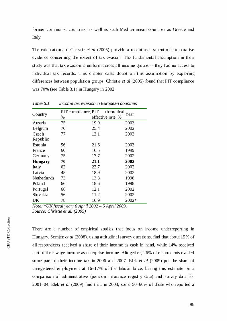
CE

UeT

DC

olle

ctio

n

98

former communist countries, as well as such Mediterranean countries as Greece and

Italy.

The calculations of Chr istie et al (2005) provide a recent assessment of comparative

evidence concerning the extent of tax evasion. The fundamental assumption in their

study was that tax evasion is uniform across all income groups -- they had no access to

individual tax records. This chapter casts doubt on this assumption by exploring

differences between population groups. Christie et al (2005) found that PIT compliance

was 70% (see Table 3.1) in Hungary in 2002.

Table 3.1. Income tax evasion in European countries

Country PIT compliance, %

PIT theoretical effective rate, % Year

Austria 75 19.0 2003 Belgium 70 25.4 2002 Czech Republic

77 12.1 2003

Estonia 56 21.6 2003 France 60 16.5 1999 Germany 75 17.7 2002 Hunga ry 70 21.1 2002 Italy 62 22.7 2002 Latvia 45 18.9 2002 Netherlands 73 13.3 1998 Poland 66 18.6 1998 Portugal 68 12.1 2002 Slovakia 56 11.2 2002 UK 78 16.9 2002* Note: *UK fiscal year: 6 April 2002 – 5 April 2003. Source: Christie et al. (2005)

There are a number of empirical studies that focus on income underreporting in

Hungary. Semjén et al (2008), using attitudinal survey questions, find that about 15% of

all respondents received a share of their income as cash in hand, while 14% received

part of their wage income as enterprise income. Altogether, 26% of respondents evaded

some part of their income tax in 2006 and 2007. Elek et al (2009) put the share of

unregistered employment at 16–17% of the labour force, basing this estimate on a

comparison of administrative (pension insurance registry data) and survey da ta for

2001–04. Elek et al (2009) find that, in 2003, some 50–60% of those who reported a

CE

UeT

DC

olle

ctio

n

99

minimum wage in fact underreported their income, and received on average about a

third of their actual income as ‘envelope wages’.

3.3 Data

Our estimation of income underreporting is based on two datasets: a random sample of

unaudited administrative tax records and the nationally representative Household

Budget Survey (HBS) of the Hungarian Central Statistical Office. Both contain data on

2005 incomes.

The sample of administrative tax records (also referred to as ‘APEH’, reflecting the

name of the tax authority) includes 227,688 individuals, or about 5.4% of all taxpayers

in the country. 4 The data refer to annual incomes from 2005. The sample size falls to

217,530 in the sample used for analysis. We top-coded the dataset by excluding those

taxpayers who had income (any type of income) above the highest value in the survey

data.5 We also excluded taxpayers with zero taxable income. 6

The HBS dataset includes 24,549 individuals in 9,058 households. The number of

individuals falls to 9,270 if we select only taxpayers and use only the working-age

population. Income data are collected from household members aged 16 and over;

demographic information is available for all members. The income reference period is

the calendar year 2005.

The tax records include

certain socio-demographic characteristics of individuals, including age, sex, post code

and, for a smaller sub-sample, the number of dependants and occupation.

7

4 There were 4.4 million taxpayers in 2005, o r 44% of the total population. Of those, 4.2 million were taxed under the progressive tax system (APEH 2006). This latter is our reference population. 5 So as to eliminate outliers from the tax audit data, we excluded taxpayers with a total income tax base of over 26.88 million Hungarian forints (HUF), wage income of over 19.67 million HUF, self-employment income of over 24 million HUF and other taxab le income of over 7.21 million HUF. The number of these excluded observations is not substantial, altogether making up about 0.2% of the sample. 6 We use a broad definition of taxab le income, including income subject to the progressive tax scheme and separately taxed self-employment income (tax base of the Simplified Business Tax is not included). Note that other separately taxed income, such as capital income, is not included in the analysis. 7 According to the National Statistical Office, h igh-income households are underrepresented and low-income households are overrepresented in the HBS, and therefore average income is somewhat underestimated by the HBS (KSH 2004: 29).

CE

UeT

DC

olle

ctio

n

100

Crucially, the results of the analysis depend on the extent to which the two datasets are

comparable in terms of both the target population and income. Our first step, therefore,

was to assess actual comparability.

The main differences between the survey data and the administrative data are as

follows: (i) HBS is based on voluntary participation, whereas it is a legal requirement

for anybody with taxable income to file a tax return; (ii) there may be under-sampling o f

high- income households in the HBS due to non-response, which would lead to

underestimating of top incomes and of the extent of inequality; (iii) incomes in the HBS

are self-reported; thus, there may be recall errors (respondents not remembering

correctly).

These features are common to all surveys, but the extent of these biases is hard to

assess. A study of Kézdi (1998) using the Income Survey of 1997 assessed the validity

of survey income by comparing self- reported earnings to incomes reported by the

employees considered to be true income. He found that the average of the self-reported

measures was 20% lower than that of the true income, and the difference was the

highest for high income groups, and the variance was also smaller by almost 30%. The

inequality of incomes measured by the Gini coefficient was also smaller within the self-

reported incomes, mostly explained by the lower self-reporting rate of higher income

individuals. As a result, the kurtosis of the distribution was higher for self-reported

measures, and distribution was skewed to the left. However, Kézdi (1998) notes that

differences within groups were not systematic. A comparative study of the self-reported

HBS and the administrative tax returns data has not yet been conducted.

Molnár (2005) had access to the pre- imputed information of the HBS and compared

them to the imputed and published dataset. He found that data was imputed for about 6-

6,5% of households, which is problematic, as most households where incomes were

imputed belonged to the first or tenth deciles after imputation.

Although these studies make the user ambiguous about the HBS, this is the only reliable

source of Hungarian households’ self-reported income with sufficient sample size and

detailed information about demographic characteristics. Therefore we decided to base

our ana lysis thereon.

CE

UeT

DC

olle

ctio

n

101

To assess the aggregate reliability of the incomes in the HBS, we checked it against the

official statistics of the National Statistical Office. The total gross employment income

of households in the HBS is 9.280 billion HUF for 2005, whereas the official statistics

for the gross employment income of households is 10.096 billion HUF (total minus the

income of those living in non-profit institutions), which shows a gap of about 8%.

Throughout the paper we assume that the income reported in the survey equals true

income and base our results on this assumption. However we shall return to the

implications of the possible failure of this assumption when discussing our results.

The HBS and the APEH data are similar in certain crucial respects: (i) both include

personal incomes with reference to the calendar year 2005, and incomes given are

annual incomes (rather than, say, monthly); (ii) information on gross income is

available in both; (iii) both datasets include basic demographic information on

respondents, includ ing sex, age, region of residence and employment status (employee

or self-employed). These features mean that the two datasets are, in fact, comparable.

We created a comparable reference population in the two datasets by (1) ensuring that

the tax record sample was representative and (2) reconciling the taxpayer population

identified in the two da tasets.

First of all, we reweighted the tax record sample on the basis of aggregate data on the

entire population of taxpayers. 8 The weights were calculated on the ba sis of region and

employment status. 9

Second, the reweighted tax sample had to be reconciled with the HBS by restricting the

latter sample to taxpayers. We thus reduced the HBS sample to those who had positive

taxable income and stated that they had filed a tax return. This provides a good

approximation of Hungarian taxpayers, because in 2005 most social incomes –

including pensions, universal family benefits and other cash transfers – were tax

exempt, unreported to the tax authorities. It also implies that pensioners are only

8 The data we used form part of a panel dataset of 2004–05, representative of the total taxpayer population of 2004. Since the taxpayer population changed somewhat from one year to the next, we reweighted the sample, based on 2005 aggregate data on the number and characteristics (region and employment) of taxpayers. 9 Our aim was to ensure that the distribution of employed and self-employed across regions was the same in the sample as in the original population. Thus we calcu lated the weights separately for the employed and the self-employed by region.

CE

UeT

DC

olle

ctio

n

102

included if they had employment income (besides pensions). The pension, however,

remained tax exempt in this case.

The definition of income compared in the two datasets is ‘gross personal taxable

income’. It is gross (i.e. before tax); it is personal rather than at household level;

therefore, it adequately reflects the individual-based Hungarian taxation system; and it

is taxable (i.e. it refers to positive income that is subject to tax). As pensions and

benefits were exempt from tax, we did not include them in our definition of taxable

income. Note that capital income other than self-employment income is not included in

the definition of income used here. 10

3.4 Methodology

We seek to assess the distributional implications of income tax evasion, which is a

result of the underreporting of income to tax authorities. In order to assess this effect,

we need to compare the distribution of True Incomes 11

Our estimation strategy is as follows: we impute individual Reported Income from tax

return data to HBS by statistical matching, calculate average Reported Income as a

and the distribution of Reported

Incomes. Our de finition of True Income includes (a) income that is not reported to the

tax authority and is thus exempt from tax and (b) those income components that are

liable to tax and are reported to the tax authority. We assume that True Income is

revealed in the income survey (HBS), and Reported Income is reported to the tax

author ity.

The main methodological problem, however, is that there is no single dataset that

includes both the True and the Reported Income of individuals: official tax return data

contain no information on undeclared and tax-exempt income, and cannot, therefore,

capture True Income; meanwhile, the survey data have no reliable information on

Reported Income. Therefore, the joint distribution of the two income measures is

unobservable.

10 Evasion of capital income might be an interesting research question, but most of this income is not included in the Household Budget Survey – probably because accurate measurement is not easy. 11 As in Smeeding and Weinberg (2001), we use the expression ‘true income’ in the sense that it accounts for the impact of the black economy (a national accounts perspective). Note that we are not able to correct for measurement error in the survey – including, for instance, the non-voluntary non-reporting of income components (e.g. not inquired about or forgotten) (Atkinson et al. (1995) use ‘true income’ in this way).

CE

UeT

DC

olle

ctio

n

103

function of individual characteristics, and then use these results to predict Synthetic

Repor ted Income in the survey da ta.

The common set of individual characteristics, (Xi), that we can use for matching is

limited. We have only three categorical variables: age group, gender, region, and

information on income of the individual. Of course, there are other characteristics that

correlate with tax evasion (for example schooling, occupational sector or household

characteristics), but these are not observed in the APEH dataset and, therefore, cannot

be used for matching.

Using only region, gender and age group (in add ition to the source of income) for

matching would not capture the dispersion of reported income within ‘cells’, that might

distort distribution, and results in a matching of poor quality, where a substantial part of

the variation in tax evasion would not be captured. To overcome this problem, we also

included income dimension to the imputation by calculating quintiles for all groups in

both datasets.

The method is the following. Using the three categorical variables available, we define

56 (4*2*7) subgroups (‘cells’). For each of these groups we calculate group quintiles,

where possible (or group average where the number of observations does not allow the

categorisation into quintiles), and for each quintile calculate average Reported Income

from the tax return data, and average True Income from the HBS. Thus, we impute

quintile specific average income for each member of the given quintile within each

‘cell’, where it was possible. 12

, , , , , , , , ,r

j k l q j k l q j k l qa y y=

Although this way we could ensure that the dispersion of

incomes within ‘cells’ is also regarded, this method relies on the assumption that peop le

do not re-rank within ‘cells’ as a result of underreporting. Including the group quint iles

as a matching variable significantly improves the quality of the matching. In Chapter

3.5, we will present evidence for this. As a last step we define adjustment factors (aj,k,l,q)

for each quintile (or group) by dividing the average Reported Income by the average

True Income.

12 For those ‘cells’ where the number of observations wasn’t sufficient to rank people in quintiles we allocated the ‘cell’ average instead of the quintile averages. The number of observations did not allow the categorization into quintiles for the self-employment income and other income. For wage income we could not allocate quintiles for females in the agegroup of 60-65 for Central Transdanubia, West Transdanubia, South Transdanubia and the North Great Plain, this is 4 groups out of the 56.

CE

UeT

DC

olle

ctio

n

104

j = Age1, Age2, Age3, Age4 k = M, F l = H, C, W, S, N, G, P q=1, 2, 3, 4, 5

where:

Age1 = 16–29 years, Age2 = 30–44 years, Age3 = 45–59 years, Age4 = 60–65

years

M = male, F = female

H = Central Hungary, C = Central Transdanubia, W = West Transdanubia, S =

South Transdanubia, N = North Hungary, G = North Great Plain, P = South

Great Plain

q=quintile within the cell

We calculate adjustment factors separately by source of income, such as wage income,

self-employment income and other taxable income. 13

In the HBS, there is some measurement error with respect to income; therefore, the

income of specific subgroups might be higher than in the tax records. To correct for this

error, we top-code adjustment factors to 1, and do not allow for over-reporting.

14

i i

rg g gy a y= ∗

We

also check the sensitivity of the estimates to top-coding by carrying out all calculations

with bo th sets of the adjustment factors (with and without top-cod ing), but regard the

top-coded results as our baseline scenario.

We then use the adjustment factors to estimate the individual Synthetic Reported

Income in the HBS: , where yr is Reported Income, y is True Income, g =

j,k,l,q stands for the groups above and gi is individual i of group g.

13 (1) Wage income refers to employees and all their employment-related income that is part of the tax base. This also includes insurance-based maternity benefits. (2) Self-employment income is the sum of wage income from self-employment and other income from self-employment, e .g. div idend income. (3) Other taxable income is the sum of all other incomes that are part of the taxable income (e.g. income from intellectual activity) except capital and other types of income that are separately taxed. 14 Instead of top-coding another option could have been to set the True Income to the Synthetic Reported Income where the adjustment factor shows overreporting. However this way a systematic b ias would have been introduced in the analysis by only correcting true income for certain cells. Therefore we decided not to do the correction of true incomes but take them as reported.

CE

UeT

DC

olle

ctio

n

105

After creating the individual Synthetic Reported Incomes in the HBS, we use a tax–

benefit microsimulation model to calculate tax liabilities based on the tax function15

( )( )( )( )

1

1'

h

h

nh i ii

n rh i ii

z y T y s

z y T y s

=

=

= − +

= − +

∑

∑

and

sum up net incomes of the household members to get (post-tax) disposable incomes.

where

hz is post-tax disposable income of household h

yi is individual True Income observed in the survey da ta r

iy is the estimated Synthetic Reported Income

T(.) is the tax func tion

s is the tax-free social income

For each household (h), we sum up the individual members of the household as (i = 1,

..,nh).

Thus, we get two disposable income measures: for the first, zh, we assume that

individuals pay tax based on their true income, for the second, zh′, we assume that they

only pay tax on their reported income. As a result, we can compare the two distributions

of household disposable incomes: F(z) and F(z′).

Our estimation may be biased for several reasons:

(i) For each member of group g, we assume the same ratio of underreporting and

therefore, underestimate the variability of z′. 16

15 On the features of the Hungarian tax policy see Appendix B. 16 Instead of assuming that tax evasion is uniform within each group and doing some linear transportation, we could assume some more complicated functional form of tax evasion – for example, that under some threshold there is no tax evasion – and do binary choice modeling. However, based on other empirical studies, we suspect that tax evasion is more complex in Hungary – i.e . tax evasion is more common at the low- and the high-income levels and less acute at middle-income levels, since civil servants (who are typically found in the middle of the distribution) tend to evade relatively little . We would need a multinomial probit estimation or some other complicated modeling to capture tax evasion behaviour within each group. The problem we face here is the small number of observations in the HBS and the small number of ind ividual characteristics we observe in the tax return data. Nevertheless, modeling the functional form of tax evasion could be a subject for future research.

However the more groups we de fine, the

CE

UeT

DC

olle

ctio

n

106

greater the standard errors of our adjustment factors (ag) will be. There is a trade-off

between these two: the more groups (g) we define, the smaller will be the first variance,

but the greater will be the second. The direction of the bias will depend on the sign of

the covariance of underreporting of true income in the HBS and the tax evasion measure

(i.e. cov(true income – reported true income in the HBS; evasion). If underreporting in

the HBS correlates with tax evasion, then our estimates will be biased upwards. If,

however, underrepor ting in the HBS is not systematic and this covariance is negative,

then the estimates will be downward biased.

(ii) Our results crucially depend on the assumption that tax evaders reveal their true

income in the income survey (HBS). Some papers (e.g. Fiorio and D’Amuri 2005)

argue for this assumption; others, especially those who use the consumption-based

approach to estimate income underreporting (e.g. Pissarides and Weber 1989; Lyssiotou

et al 2004), suppose that income in surveys is underreported. But even these studies use

a group of individuals as a reference population and assume that this reference

population does not underreport survey income. Normally, the reference population is

the employed, and researchers calculate income underreporting among the self-

employed in compa rison. We assume that survey incomes are ‘true’ in the sense that

there is no financial incentive to conceal income in an anonymous survey.

However we should recall that Kézdi (1998) and Molnár (2005) found incomes to be

underreported in Hungarian household surveys, Kézdi (1998) estimated this

underreporting to 20%. Should income be partly concealed in the HBS our figures for

underreporting will be lower bound estimates. If high income individuals conceal a

greater share of their income, as Kézdi (1998) found, the estimated underreporting will

be more downward biased for these high income groups.

Another issue is the correlation of measurement error between household members.

Although we cannot use information on the household in the imputation, underreporting

is likely to be correlated across household members. If individual income of household

members are similar then the bias will essentially the same as presented. However if

household members have different individual incomes, e.g. the head of household

belongs to the top while his or her spouse to the low or middle income groups, then this

omitted information will cause further biases. Depending in the actual structure of the

intra-household income distribution the bias in the middle income groups might be

CE

UeT

DC

olle

ctio

n

107

higher and proportionately the difference between the high, and the low/middle income

groups might be smaller then suggested above.

(iii) The two datasets contain data from different individuals who only share a few

characteristics. Although we have two random samples of the same underlying

population, there is sampling error in both datasets, which will bias our results. As

already discussed above, the HBS sample underestimates the aggregate gross

employment income of the population by about 8%. The APEH dataset is a 5% sample

of the total taxpayer population; therefore, the sampling error is significantly smaller. In

fact, we did not find a significant difference between the aggregate and the sample

based aggregate income measures. Since the True Income measures based on the HBS

are probably underestimated the calculated underreporting will be downward biased.

The distribution of the Synthetic and the actual Reported Income of taxpayers is shown

in Figure 3.1. The synthetic distribution overlaps with the distribution of Reported

Income coming from the APEH dataset for the bottom eight deciles, but, as expected, it

underestimates the actual distribution of taxable income among high- income taxpayers.

The average Reported Income, Synthetic Reported Income and the corresponding

confidence intervals by region, gender and age group are presented in Appendix D.

When comparing the reported income measures based on the two da tasets we see that in

the not-topcoded case most p-values are high: in 34 out of the 56 groups the p-value is

90% or more (for 44 out of the 56 groups the p-value is above 80%). For these groups

we cannot reject the hypot hesis that the HBS and the APEH group averages are equal.

For the top-coded case however the p-values are significantly lower. It is only 5 groups

out of the 56 where the p-values are above 80%.

CE

UeT

DC

olle

ctio

n

108

Figure 3.1 Distribution of the synthetic (HBS) and actual (APEH) reported income

Note: own calculations based on 2005 HBS and APEH tax returns.

(iv) Choice of functional form of tax evasion might also bias our results. We assume

that tax evasion is uniform within each group that is a linear transportation in essence.

Based on other empirical studies, we suspect that tax evasion is more complex in

Hungary: i.e. tax evasion is more common at the low- and the high- income levels and

less acute at middle- income levels, since civil servants (who are typically found in the

middle of the distribution) tend to evade relatively little. However, the small number of

observations in the HBS and the small number of individual characteristics we observe

in the tax return data does not allow a more complex modeling of the tax evasion

function within cells without increasing the standard errors of the adjustment factors to

a very high degree. The possible implications of the greater share of underreporting of

high income individuals have been discussed under point (ii).

3.5 Results: Extent of under-reporting

According to our calculations, income underreporting runs at 8-18% on average (see

Table 3.2). The extent of income underreporting varies across income groups, but is at

0 2000 4000

6000 8000

10000 12000

14000 16000

0 1 2 3 4 5 6 7 8 9 10 deciles of taxpayers

‘000

HU

F synthetic reported income (HBS) actual reported income (APEH)

CE

UeT

DC

olle

ctio

n

109

its highest in the three poorest deciles (ranging from 17% to 27%) and in the richest

decile (21%). Thus, the poor benefit most from income tax evasion in proportion to

their income, while the rich benefit most in purely monetary terms.

Table 3.2. Underreporting of taxpayers by level of income under different specifications

Income decile of taxpayers by True Income

True Income Rate of underreporting

(1) Underreporting not top-coded

(2) Underreporting

top-coded 1 (poorest) 302 -17% 17% 2 696 17% 24% 3 899 17% 21% 4 1075 17% 19% 5 1250 14% 18% 6 1436 13% 18% 7 1693 9% 14% 8 2020 3% 13% 9 2578 1% 14% 10 (richest) 4574 6% 21% Total 1691 8% 18% Notes: Underreporting = (True Income - Reported Income)/True Income Reported Income = Adjustment Factor * True Income Top-coded means that adjustment factors are maximized to 1, not allowing for income over-reporting. Mean income by income group is annual gross personal income in thousand forints. True Income is as observed in the HBS dataset. Income quantiles of taxpayers were generated on the basis of True Income, excluding those earning zero or negative incomes.

We used two different sets of adjustment factors. First, we allowed the income of

certain subgroups to be higher in the tax records than in the income survey (‘not top-

coded’). Second, we top-coded our adjustment factors to 1 and did not allow over-

reporting (‘top-coded’).

CE

UeT

DC

olle

ctio

n

110

We find that underreporting is quite different for different population groups. The self-

employed 17

Tax evasion is higher among men, which is likely to be associated with differences in

risk aversion: women are usually more risk averse, which reduces income

underrepor ting. Our calculations also show that men underrepo rt bot h wage income and

self-employment income mor e than women do. We also found that the elde rly

(especially those around retirement age) underrepo rt more than younger age groups

do.

tend to underreport the most: about two-thirds (65%) of the ir income is not

reported as a tax base to the tax authority. By contrast, employees generally comply

with tax rules, with an overall rate of underreporting of 4% (Table 3.3). Other income is

underreported by 8%. These results are in line with, e.g., Slemrod (2007), who reported

that based on tax audit data, non-business income in the US was underreported by 4%,

whereas business income on average was underreported by 43%. Within this latter the

nonfarm proprietor income underreporting was 57%.

Underreporting is highest in the highest- income region – Central Hungary (including

the capital, Budapest). One explanation for this might be the region’s greater share of

economic sectors that are particularly prone to tax evasion: much of the construction

industry and the service sector are to be found in and around the capital. In terms of

underreporting, Central Hungary is followed by a rich region (West Transdanubia) and

a poor one (South Great Plain). The rates for underreporting are 12%.

18

17 We define the self-employed as those who earned at least 1 HUF from any kind of self-employment in the reference period. 18 The difference between the rates of underreporting by age groups is statistically significant.

A study of the situation in Estonia (Kriz et al 2007) came up with similar findings:

men and the elderly are more likely to evade payroll and income taxes. Basing his

investigation on a specific survey in Hungary, Tóth (2008) also found that men tend to

underreport wages more than women do.

CE

UeT

DC

olle

ctio

n

111

Table 3.3. Underreporting by main source of income, region, age and gender

Population share True Income

Synthetic Reported Income

Underreporting

Main income source

Wages/salaries 90% 1630 1569 4% Self-employment 10% 2490 883 65% Region Central Hungary 31% 2189 1802 18% Central Transdanubia

11% 1507 1391 8%

West Transdanubia 12% 1646 1441 12% South Transdanubia

7% 1432 1305 9%

North Hungary 12% 1468 1390 5% North Great Plain 13% 1440 1315 9% South Great Plain 14% 1529 1341 12% Gender Male 50% 1946 1615 17% Female 50% 1488 1385 7% Age group 16–29 18% 1299 1175 10% 30–44 39% 1766 1516 14% 45–59 41% 1850 1631 12% 60–65 2% 1867 1474 21% Notes: Underreporting = (True Income - Reported Income)/True Income Reported Income = Adjustment Factor * True Income Here we present results for the case where adjustment factors are top-coded. Top-coding means that adjustment factors are maximized to 1, not allowing for income over-reporting. Mean income by income group is annual gross personal income in thousand forints. True Income is true taxable income as observed in the HBS dataset.

Comparison of results with and without group quintiles as matching variable

As ment ioned in the Methodo logy, it is not straightforward whether including the

quintiles within the 56 cells as a matching variable is necessary. Although in general it

is better to include more matching variables, however if the more variables do not

significantly improve the quality, then only extra noise is added to the estimation.

Therefore it is essential to check if adding the income information to the matching

improves the quality.

CE

UeT

DC

olle

ctio

n

112

First, Table 3.4 compares income underreporting with and without using the income

quintile information as a matching variable. In the first two columns underreporting is

presented by income deciles when only the region, age group and gender variables are

used for matching, and in the last two columns we present our baseline case, where also

group quintile information is used. 19

19 Recall that with in-group quintiles can only be used as a matching variab le for the wage income as for self-employment and other income the number of observations is insufficient.

Average income underreporting is somewhat different if we leave out the quintile

averages as a matching variable. In the top-coded specification, the difference is

substantial: 13% versus 18% of underreporting whereas for the not-topcoded case the

difference is rather small: 9% versus 8%. The distribution of underreporting by income

levels changes substantially if we include the quintile averages as a matching variable. It

lowers underreporting in the bottom two deciles from 25-30% to 17-24%.

Underreporting becomes higher in the middle income groups: from 8-14% to 13-19%.

In the 8-9 deciles, underreporting again becomes lower when including the quintile

averages from 8-13% to 1-14%. Including quintile averages has a different effect on the

distribution of underreporting in the top-coded and not-topcoded cases.

Although the magnitude of underreporting is somewhat different in the deciles with the

two sets of matching variables, the main finding that income underreporting has a U-

shape (highest for the low and high income groups) remained unchanged.

CE

UeT

DC

olle

ctio

n

113

Table 3.4. Underreporting of taxpayers by level of income

Income decile of taxpayers by True Income

Rate of underreporting – using region, agegroup and gender for matching

Rate of underreporting – using region, agegroup, gender and group quintiles for matching

(1) Underreporting not top-coded

(2) Underreporting

top-coded

(1) Underreporting not top-coded

(2) Underreporting

top-coded 1 (poorest) 26% 30% -17% 17% 2 25% 29% 17% 24% 3 14% 18% 17% 21% 4 10% 14% 17% 19% 5 9% 13% 14% 18% 6 8% 12% 13% 18% 7 9% 13% 9% 14% 8 8% 12% 3% 13% 9 10% 13% 1% 14% 10 (richest) 13% 16% 6% 21% Total 9% 13% 8% 18% Notes: Underreporting = (True Income - Reported Income)/True Income Reported Income = Adjustment Factor * True Income Top-coded means that adjustment factors are maximized to 1, not allowing for income over-reporting. Mean income by income group is annual gross personal income in thousand forints. True Income is as observed in the HBS dataset. Income quintiles of taxpayers were generated on the basis of True Income, excluding those earning zero or negative incomes.

As Tables E.1 and E.2. in Appendix E shows in case of adding the group quintiles as a

matching variable, the adjustment factors display substantial heterogeneity between the

56 cells (by region, gender and age group). The average distance between the

adjustment factors in the lowest and the highest income quintiles are rather different by

the 56 groups. It varies between 0 and 8,7 for the not top-coded case and between 1 and

7,2 for the top-coded case. On average, it is the lowest in North Hungary (1,45) and

highest in Central Hungary (3) for the not top-coded case (lowest in North Hungary and

highest in South Great Plain for the top-coded case). It shows that the inc lusion of this

information captures a great heterogeneity in the sample therefore it is an important

matching variable. We can conclude that, although the main findings are robust to the

exclusion of this matching variable, the quality of the matching is significantly

improved by the inclus ion.

CE

UeT

DC

olle

ctio

n

114

3.6 Results: Distributional implications

In order to reveal the effects of tax evasion on progressivity and the distribution of

incomes, we use a tax–benefit microsimulation model20

( )ri i iz y T y s= − +

that takes into account

interactions between the elements of the tax and benefit system and household

members. The total Synthetic Reported Income for each individual comprises the sum

of the synthetic reported wage income, synthetic reported self-employment income and

synthetic reported other income.

Although income underreporting happens at the individual level due to the personal

income tax system, the effects on the income distribution can only be measured at the

household level. Total household disposable income depends on the true income of each

household member. Income underreporting as such modifies total household income,

but the impact is largely dependent on the tax system and on the system of cash

benefits. The use of a tax–benefit model allows us to take account of the complexity of

the tax system, including the fact that only some income components are subject to tax

as well as the potential interaction between specific cash benefit and tax policies

(benefit entitlements may also change as a result of tax evasion).

As was discussed in the section on methodo logy, we aim to estimate the effect of tax

evasion on the distribution of disposable ‘net income’. We calculate net income thus:

where zi is total personal disposable income for individual i; yi is individual True

Income; riy is Reported Income; T(.) is the tax function; and s is the tax-free social

transfers received by individual i. We then sum up net incomes of the household

members to get (post-tax) disposable incomes:

( )( )1hn r

h i iiz y T y s

== − +∑

20 For simulation purposes, we use some of the Stata algorithms of HKFSZIM, a microsimulation model that was developed and programmed in the Ministry of Finance and the Office of the Fiscal Council. We programmed the 2005 Hungarian tax and benefit rules. We use HBS as representative data for the population.

CE

UeT

DC

olle

ctio

n

115

Note that, in Hungary, soc ial transfers (s) are untaxed – with the exception of insurance-

based maternity benefits, which are included in labour income.

We now present the findings of our microsimulation. In this section, we model all major

direct tax and cash benefit policies in 2005 and consider their interactions, based on the

HBS. Using our adjustment factors for income underreporting, we are able to assess the

impact of tax evasion on household incomes and their distribution (aga inst the

hypothetical counterfactual of full compliance).

Table 3.5. Fiscal and distributional implications of tax evasion

Underreporting not top-coded

Underreporting top-coded

Full compliance

Tax evasion

Difference Tax evasion Difference

Average equivalised PIT payment by households (HUF, annual) 209 897 192 801 -8,1% 167 083 -20,4% Poverty line (HUF, monthly) 46 649 46 713 0,1% 47 524 1,9% Poverty rate (FGT a=0) 0,11 0,11 1,5% 0,12 5,7% Poverty gap (FGT a=1) 0,03 0,03 2,4% 0,03 4,0% Gini 0,26 0,27 3,7% 0,28 6,7% P90/P10 3,17 3,21 1,2% 3,37 6,3% P75/P25 1,79 1,79 0,2% 1,82 1,6% P90/P50 1,83 1,85 1,0% 1,92 5,0% Atkinson e=0.5 0,06 0,06 10,1% 0,07 15,2% Atkinson e=2 0,22 0,23 4,8% 0,24 9,0% Kakwani 0,33 0,32 -0,2% 0,31 -5,2% Reynolds-Smolensky 0,07 0,05 -20,6% 0,04 -46,2% Suits 0,37 0,36 -2,2% 0,34 -8,1% Notes: full compliance provides estimates of income tax variables, assuming that true incomes as observed in the HBS are reported to the tax authorities. Tax evasion provides estimates of the same variables, assuming incomes are underreported to the tax authorities by the adjustment factors (region, sex, etc.). FGT refers to the Foster Greer Thorbecke family of poverty indices. Income concept: equivalized household income, annual. For a detailed description of the above measures see Appendix A.

The limitations of our model are that, for specific income types, the number of

observations is very small; for some others, there are measurement errors (e.g. property

incomes, agricultural incomes, intellectual activities). Certain specific tax rules

(especially tax credits) are simplified in the model, as there is no adequate information

in the HBS (e.g. on donations to charities). These modelling features are unlikely to

affect the estimated implications of tax evasion, since the expectation is that they have a

CE

UeT

DC

olle

ctio

n

116

similar impact on the results under both the full compliance scenario and the tax evasion

scenario.

If underreporting increases by income, the statistical matching procedure that we follow

somewhat dampens the distributive effects of underreporting. In order to minimise this

effect, we have included the income quintiles within cells as a matching variable and

took account of the increasing rate of underreporting with income.

The fiscal implications of tax evasion are substantial: the average PIT burden of

households is 8–20% lower because of income underreporting.

Income inequality and poverty are significantly higher with tax evasion. The Gini

coefficient increases by 4–7% and the P90/P10 ratio by 1–6%. Similarly, the Atkinson

index rises for both alternative values of the inequality aversion parameter.21

We have the revisit the problem of underreporting in the HBS when evaluating the

results. Recall that Kézdi (1998) estimated that underreporting in a household survey

was around 20% in 1997. Both Kézdi (1998) and Molnár (2005) concluded that

underreporting was higher in high income groups. If these problems are present at the

2005 HBS then income underreporting is in fact greater than the estimated 8-18%

calculated by our method. Should underreporting in the HBS be still around 20% than

The

poverty line rises by around 2%, whereas the poverty rate and poverty gap increase by

about 2-6%.

Tax evasion reduces the progressivity of the income tax system quite subs tantially. The

Kakwani and the Suits indices indicate a decline of up to 8%, while the redistributive

effect of the tax system as measured by the Reynolds-Smolensky index falls

significantly as well. In these calculations, we consider the impact of both personal

income taxes and soc ial security contributions – in other words, all taxes on labour at

the employee level. The fall in progressivity is a consequence of the relatively higher

level of income underreporting among high- income groups (as we indicated earlier, the

underreporting of low-income groups is higher than average, but most of these are taxed

at a low or zero effective tax rate).

21 Note that the extent of the change is greater when the inequality aversion parameter is smaller (e=0.5), when less weight is attached by society to redistribution to the poor. (The potential range of e is from 0, which means that the society is indifferent to redistribution, to infinity, where the society is concerned only with the position of the poorest income group.)

CE

UeT

DC

olle

ctio

n

117

the estimated total underreporting will increase by this magnitude. However in lack of

more recent results it is impossible to tell the magnitude of the bias of our results.

Underreporting in the HBS would also have implications for the fiscal and distributional

effects of underreporting. If high income groups underreport more in the HBS, as Kézdi

(1998) found, then both the personal income tax gap and the increase in poverty

measures and progressivity will increase. Again, in lack of the exact measures the extent

of this bias is impossible to estimate, it greatly depends on the relative differences

between low, middle and high income groups. However, in this case our results will

surely be downwards biased. If we accept Molnár’s (2005) finding that misreporting of

incomes was the highest among low and high income groups then the implications are

more difficult to assess. Since low income groups pay PIT with a low effective rate the

PIT gap will still be downwards biased, but the poverty and progressivity implications

depend on the relative measures between low and high income groups. If low income

groups underrepo rt in the HBS to a higher share than high income groups than the

change in poverty rates and progressivity might be lower than our estimates. If high

income groups underreport a greater share than low income groups that these estimates

will be downward biased too.

Policy implications

We found that income underreporting is highest in the three poorest deciles (ranging

from 17% to 24%) and in the richest decile, surpassing income underreporting by

middle-to-high income groups. A similar U-shape was found in Greece by Matsaganis

and Flevotomou (2008) and in the US by Johns and Slemrod (2008). Note that owing to

the progressive tax scheme and tax allowances, the effective tax rate is greater for those

with high incomes, while wage income at or around the minimum wage is virtually tax

free.

Compared to other countries, estimated tax evasion in Hungary is quite high, but not

outstandingly so. In Greece, the tax gap with respect to personal income taxes was

found to be 25% (Matsaganis and Flevotomou, 2008). In the USA, the tax gap (taking

account of all federal taxes, rather than just income tax, as in our case) was estimated to

CE

UeT

DC

olle

ctio

n

118

be 17% in the early 1990s and was found to be relatively unchanged over the previous

20 years (Andreoni et al, 1998). A third of US taxpayers were found to underreport their

income.

Should Hungarian policymakers turn a blind eye to (or even connive at) the high rate of

underreporting in the lowest three deciles? There may be a case based on equity for

tolerating tax evasion. ‘If the poor had more oppor tunity of evading taxes than the rich,

or were better at it […] then the egalitarian policy maker might have good reason to

smile indulgently on evasion: up to a point anyway’ (Cowell, 1985:185). Note,

however, that there is a high share of the self-employed among those with low incomes.

According to our calculations, around half of the self-employed have incomes at or

below the level of the minimum wage. The self-employed have greater opportunity than

wage earners to underreport their incomes, even in countries with high tax morale – a

fact that hampers horizontal equity.

An important implication of our findings is that, since tax evasion is not uniform across

the various social groups, the tax author ities can target certain groups for audit, thus

improving their efficiency. We make no assessment in this study of how taxpayers

might react to po licy changes.

3.7 Conclusions

This chapter has estimated the inc idence of income tax evasion in Hungary using a

random sample of the administrative tax records of around 230,000 individuals, not

hitherto accessible to researchers. Gross incomes declared in the administrative tax

returns are compared with those declared in the HBS (a nationally representative

income survey), on the assumption that tax evaders are more likely to report their true

income in the course of an anonymous interview. We have estimated income

underreporting among those people who declared at least some income to the tax

authorities, leaving out those individuals who did not declare any income. The method

we have applied provides the first microdata-based estimates for personal income tax

evasion in Hungary.

Our estimates show that the average rate of underreporting is 8–18%, though this

conceals big variations be tween the self-employed (who conceal around two-thirds of

CE

UeT

DC

olle

ctio

n

119

their income) and employees. Men are more likely to hide their incomes than are

women, probably because they are less risk averse than women. The rate of

underreporting is found to be highest among taxpayers at the bottom and the top ends of

the distribution. Thanks to the progressive tax scheme and tax allowances, the effective

tax rate is quite different at the low and high income levels: high- income earners face

high e ffective tax rates, while wage income at or around the minimum wage is basically

tax free. Therefore, the similar rate of underreporting implies quite different actual tax

payments at the two ends of income distribution. Because of the progressivity of the tax

system, evasion by top earners has more of an impact on the state budget.

Using the estimated rates of underreporting, we use a tax–benefit microsimulation

model to simulate the tax payment and disposable income of households. We calculate

the distributional implications of underreporting by comparing the scenarios of full

compliance and tax evasion, taking account all major direct taxes and cash benefits, as

well as the way they interact with one another. Tax evasion reduces households’

average personal income tax payment of by 8-20%. The poverty rate and income

inequality are higher when taking account of underreporting, which shows that high

earners tend to evade more in absolute terms. In the scenario that takes account of tax

evasion, the progressivity of the tax system is lower than intended.

In the policy debate, tax evasion is often attributed exclusively to the high level of taxes

in Hungary, or else to a culture of ‘free-riding’ by citizens. Policymakers tend to be

concerned primarily with the fiscal loss that results from tax evasion. Our results

contribute a new aspect to this debate: since effective tax rates are higher for high

earners, their income underreporting reduces progressivity. The reduced progressivity of

the income tax scheme is likely to alter the social outcomes of the policies pursued, and

this may undermine the equity of income redistribution. We have also shown that

specific rates of tax evasion vary subs tantially by soc ial group, and that these

differences alter income inequality, poverty and tax progressivity. As long as tax

evasion persists, informed policy decisions that seek to promote social welfare need to

consider its implications. More knowledge of the magnitude of tax evasion is thus

essential if government wishes to evaluate the redistributive effect of taxes, either over

time or after certain fiscal reforms.

CE

UeT

DC

olle

ctio

n

120

Bibliography

Andreoni, J., B. Erard and J. Feinstein (1998). “Tax Compliance.” Journal of Economic

Literature 36(2): 818–860.

APEH (2006). Az APEH világa 2006. évkönyv [APEH Bulletin 2006] Budapest,

APEH.

Atkinson, A. B., L. Rainwater and T. M Smeeding (1995). “Income Distribution in

OECD Countries: The Evidence from the Luxembourg Income Study (LIS).”

Social Policy Studies, No.18. Paris: OECD.

Beron, K. J., H. V. Tauchen and A. V. Witte (1992). ‘The effect of audits and

socioeconomic variables on compliance’. In: Why People Pay Taxes. (ed. J.

Slemrod ) Ann Arbor: University of Michigan Press.

Bloomquist, Kim M. (2003) “U.S. Income Inequality and Tax Evasion: A Synthesis,”

Tax Notes International 31(4): 347-367.

Christie, E., M. Holzner and M. Lacko (2005). “Taxation and the Shadow Economy in

Europe.” OeNB Jubiläumsfondsproject No. 10867. Vienna: Vienna Institute for

International Economic Studies.

Cowell, F. (1985). “The economic analysis of tax evasion”. Bulletin of Economic

Research 37(3): 163-189.

Elek, P., A. Scharle, B. Szabó and P. A. Szabó (2009). “A feketefoglalkoztatás mértéke

Magyarországon [Employment in the black economy in Hungary]”. In: Shadow

Economy. (eds. A. Semjén and I. J. Tóth) Budapest: MTA-KTI, pp. 84–102.

European Commission (2007). Taxation Trends in the European Union. Luxembourg:

Publications Office of the European Union.

Fiorio, C. and F. D’Amuri (2005). “Workers’ tax evasion in Italy.” Giornale degli

Economisti e Annali di Economia 64(2/3).

Freire-Serén, M. J and J. Panadés (2008). “Does tax evasion modify the redistributive

effect of tax progressivity?” Economic Record 84(267): 486–495.

Hanousek, J. and F. Palda (2004). “Quality of government services and the civic duty to

pay taxes in the Czech and Slovak Republics, and other transition countries.”

Kyklos 57(2): 237–252.

CE

UeT

DC

olle

ctio

n

121

Johns, A. and J. Slemrod (2008), "The Distribution of Income Tax Noncompliance",

Working Paper, University of Michigan, September 12, 2008

Kézdi, G. (1998). “Az önbevalláson alapuló kereseti adatok érvényessége [The validity

of self-reported earnings].” Közgazdasági Szemle 45(11): 1035–1042

Kriz, K. A., J. Meriküll, A. Paulus and K. Staehr (2007). “Why Do Individuals Evade

Payroll and Income Taxation in Estonia?” Faculty of Economics and Business

Administration Working Paper Series, No. 49. Tartu: University of Tartu.

KSH (2004). “Háztartás-statisztikai közlemények [Reports on Household Statistics].”

No. 25, 2004/I. Budapest: Központi Statisztikai Hivatal.

Lyssiotou, P., P. Pashardes and T. Stengos (2004). “Estimates of the black economy

based on consumer demand approaches.” Economic Journal 114(497): 622–640.

Matsaganis, M. and M. Flevotomou (2008). “Distributional implications of income tax

evasion: The case of Greece.” Manuscript.

Molnár, Gy. (2005). “Az adatállomány és a rotációs panel [The dataset and the

rotational panel].” In: A magyar háztartások jövedelmi és fogyasztási mobilitása

az ezredfordulón [Income and consumption mobility of Hungarian households at

the millenium]. (eds. Zs. Kapitány, Gy. Molnár and I. Virág): 139-147.

Persson, M. and P. Wissén (1984). “Redistribut ional aspects of tax evasion.”

Scandinavian Journal of Economics 86(2): 131–149.

Pissarides, C. and G. Weber (1989). “An expenditure-based estimate of Britain’s black

economy.” Journal of Public Economics 39(1): 17–32.

Slemrod, J. (2007). “Cheating ourselves: The economics of Tax Evasion.” Journal of

Economic Perspectives 21(1): 25–48.

Schneider, F. and D. H. Enste (2000). “Shadow economies: Sizes, causes, and

consequences.” Journal of Economic Literature 38(1): 77–114.

Schneider, F. and R. Klinglmair (2004). “Shadow Economies around the World: What

do we Know?” CESifo Working Paper No. 1167 and IZA Discussion Paper No.

1043. University of Linz.

Semjén, A., I. J. Tóth, M. Medgyesi and Á. Czibik (2008). “Tax Evasion and

Corruption: Population Involvement and Acceptance. Survey results.”

Discussion paper of the Institute of Economics DP-2008/13.

Smeeding, T. M. and D. H. Weinberg (2001). “Toward a uniform definition of

household income.” Review of Income and Wealth 47(1) : 1–24.

CE

UeT

DC

olle

ctio

n

122

Tóth. I. J. (2008). “Be nem jelentett munkavégzés Magyarországon – elterjedtség és

társadalmi összetevők [Unregistered employment in Hungary – size and social

causes].” Conference presentation, ILO Tripartite Conference, 8 December

2008, Budapest.

CE

UeT

DC

olle

ctio

n

123

Appendix

A. Definitions

Our de finition of gross taxable income based on variables in the Household Budget

Survey:

- Gross income from main employment (munkáltatótól, főállású munka viszonyból származó bruttó jövedelem)

Wage income

- Gross income from secondary employment (másodállásból, mellékfoglalkozásból származó jövedelem)

- Maternity benefit (gyed)

- Childbirth benefit (terhességi gyermekágyi segély)

- Labour income from self-employment (egyéni vagy társas vállalkozásból származó jövedelem (kivét, munkabér címén))

Self-employment income

- Other entrepreneurial income that is part of the aggregate tax base (összevont adóa lapba tartozó vállalkozói jövedelmek)

- Other entrepreneurial income that is not part of the aggregate tax base (nem összevont adóa lapba tartozó vállalkozói jövedelmek)

- Redundancy pay (végkielégítés összege)

Other income that is part of the aggregate tax base

- One-off contract payment (egyszeri megbízásból származó jövedelem)

- Income from intellectual activity (szellemi alkotásból származó jövedelem)

- Tips (borravaló, hálapénz)

CE

UeT

DC

olle

ctio

n

124

All poverty and progressivity measures are calculated using Stata programme by own

programming and with the Stata codes

povdeco (http://ideas.repec.org/c/boc/bocode/s366004.html by S. Jenkins)

ineqdeco (http://ideas.repec.org/c/boc/bocode/s366002.html by S. Jenkins) and

progres (http://ideas.repec.org/c/boc/bocode/s456867.html by A. Peichl and P. Van

Kerm)

- Poverty line is a relative measure, 60% of the median equivalised household income

- Poverty rate (FGT a=0) is a headcount ratio, the number of persons below the poverty line divided by the number of persons in the total population, a poverty index from the Foster, Greer and Thorbecke (1984) class

- Poverty gap (FGT a=1) measures the mean aggregate income shortfall relative to the poverty line across the whole population, where the non-poor have a shortfall of zero, also a poverty index from the Foster, Greer and Thorbecke (1984) class

- The Gini coefficient is a measure of the inequality of distribution, takes a value of 0 when total equality and 1 when total inequality. I t is calculated based on the Lorenz curve measuring the ratio of the area between the line of equality and the Lorenz curve

- P90/P10, P75/P25 and P90/P50 are ratios of percentile measures of the income distribution, P90, P75, P50, P25 and P10 standing for the 90th, 75th, 50th, 25th and 10th percentile respectively

- The Atkinson indices are inequality indices, where in A(e) e is the inequality aversion parameter. The more positive e > 0 is, the more sensitive A(e) is to income differences at the bottom of the distribution.

- The Kakwani index is a measure of tax progressivity defined as twice the area between the taxpayment’s concentration curve and the Lorenz curve.

- The Reynold-Smolenski index measures the difference between the Gini coefficients of the pre-tax and the post-tax incomes.

- The Suit index compares the cumulative share of income received by taxpayers, ordered from lowest to highest, to their cumulative share of taxes paid: S = 1- L/K where K denotes the area below the line of proportionality, and L denotes the area below the Lorenz curve of tax payments against income

CE

UeT

DC

olle

ctio

n

125

B. Features of Hungarian tax policy

The income tax system is subject to frequent (mostly annual) change, bo th to the tax

rates and to the tax brackets. Some of this might be explained by the indexation to

inflation; but in most cases the changes reflect changing policy priorities, which

sometimes focus on raising revenue and a t other times on lowering t he tax burden.

Table B1. Personal income tax brackets (in HUF) and rates

2003 2004 2005 2006 Tax bracket Rate Tax bracket Rate Tax bracket Rate Tax bracket Rate 0–650,000 20% 0–800,000 18% 0–1,500,000 18% 0–1,550,000 18% 650,001–1,350,000

30% 800,001–1,500,000

26%

1,350,001– 40% 1,500,001– 38% 1,500,001– 38% 1,550,001– 36%

As well as PIT, in 2004 employers had to pay a total of 32% in social security

contributions on labour incomes. Employee social security contributions amounted to

13.5%. These rates were relatively stable and remained the same between 2004 and

2006.

Budget revenue from personal income taxes made up 6.6% of GDP in 2005 (European

Commission 2007 ). The Hungarian budget, however, relies heavily on indirect taxes,

and in 2005 received some 53% more from VAT than from PIT.22

22 Ministry of Finance, Hungary, balance sheet of the central government annual budget. Downloaded on 14 January 2009 from

With respect to the distribution of the tax burden in the country: in 2005 about a third o f

taxpayers paid the higher marginal tax rate of 38% on some of their total income.

www.pm.gov.hu

CE

UeT

DC

olle

ctio

n

126

C. Descriptive and summary statistics

Table C1. Main characteristics of the taxpayers in the administrative and survey datasets

Number of observations APEH HBS

Region Employed Self-empl. Total Region Employed

Self-empl. Total

Central Hungary 55097 3465 58562 Central Hungary 2463 373 2836 Central Transdanubia 18632 1279 19911

Central Transdanubia 961 86 1047

West Transdanubia 18017 1266 19283 West Transdanubia 990 123 1113 South Transdanubia 21320 1314 22634

South Transdanubia 626 54 680

North Hungary 18977 1148 20125 North Hungary 1067 78 1145 North Great Plain 24161 1650 25811 North Great Plain 1092 101 1193 South Great Plain 21556 1577 23133 South Great Plain 1138 118 1256 Total 177760 11699 189459 Total 8337 933 9270 Share (%)

APEH Employed Self-empl. Total HBS Employed

Self-empl. Total

Central Hungary 29% 2% 31% Central Hungary 27% 4% 31% Central Transdanubia 10% 1% 11%

Central Transdanubia 10% 1% 11%

West Transdanubia 10% 1% 10% West Transdanubia 11% 1% 12% South Transdanubia 11% 1% 12%

South Transdanubia 7% 1% 7%

North Hungary 10% 1% 11% North Hungary 12% 1% 12% North Great Plain 13% 1% 14% North Great Plain 12% 1% 13% South Great Plain 11% 1% 12% South Great Plain 12% 1% 14% Total 94% 6% 100% Total 90% 10% 100% Number of observations

APEH Employed Self-empl. Total HBS Employed

Self-empl. Total

Male 95606 8203 103809 Male 3996 624 4620 Female 108201 5520 113721 Female 4341 309 4650 Total 203807 13723 217530 Total 8337 933 9270 Share (%)

APEH Employed Self-empl. Total HBS Employed

Self-empl. Total

Male 44% 4% 48% Male 43% 7% 50% Female 50% 3% 52% Female 47% 3% 50% Total 94% 6% 100% Total 90% 10% 100% Notes: APEH: administrative data from the tax authority, HBS: Household Budget Survey.

CE

UeT

DC

olle

ctio

n

127

Table C2. Number and share of observations in each cells by the three variables (region, gender, age group) and by employment status in the administrative and survey datasets

HBS 15-29 30-44 45-59 60+ Employee Male female male female male female Male female Total

Central Hungary 224 266 430 486 441 563 31 22 2463

Central Transd. 105 111 160 174 173 225 10 3 961 West Transd. 108 114 203 178 179 193 11 4 990 South Transdan. 60 43 123 120 127 144 6 3 626 North Hungary 85 77 224 206 230 235 6 4 1067 North Great Pl. 101 113 217 238 170 236 7 10 1092 South Great Pl. 99 118 235 241 221 206 10 8 1138 Entrepreneur

Central Hungary 22 6 106 47 95 80 14 3 373

Central Transd. 6 1 27 14 27 9 1 1 86 West Transd. 12 2 35 13 40 20 1 0 123 South Transdan. 5 2 14 3 22 7 1 0 54 North Hungary 1 2 20 16 25 14 0 0 78 North Great Pl. 4 6 35 11 30 13 2 0 101 South Great Pl. 7 1 30 14 40 22 2 2 118 9270 15-29 30-44 45-59 60+ Employee male female male female male female Male female

Central Hungary 2,42% 2,87% 4,64% 5,24% 4,76% 6,07% 0,33% 0,24%

Central Transd. 1,13% 1,20% 1,73% 1,88% 1,87% 2,43% 0,11% 0,03% West Transd. 1,17% 1,23% 2,19% 1,92% 1,93% 2,08% 0,12% 0,04% South Transdan. 0,65% 0,46% 1,33% 1,29% 1,37% 1,55% 0,06% 0,03% North Hungary 0,92% 0,83% 2,42% 2,22% 2,48% 2,54% 0,06% 0,04% North Great Pl. 1,09% 1,22% 2,34% 2,57% 1,83% 2,55% 0,08% 0,11% South Great Pl. 1,07% 1,27% 2,54% 2,60% 2,38% 2,22% 0,11% 0,09% Entrepreneur

Central Hungary 0,24% 0,06% 1,14% 0,51% 1,02% 0,86% 0,15% 0,03%

Central Transd. 0,06% 0,01% 0,29% 0,15% 0,29% 0,10% 0,01% 0,01% West Transd. 0,13% 0,02% 0,38% 0,14% 0,43% 0,22% 0,01% 0,00% South Transdan. 0,05% 0,02% 0,15% 0,03% 0,24% 0,08% 0,01% 0,00% North Hungary 0,01% 0,02% 0,22% 0,17% 0,27% 0,15% 0,00% 0,00% North Great Pl. 0,04% 0,06% 0,38% 0,12% 0,32% 0,14% 0,02% 0,00% South Great Pl. 0,08% 0,01% 0,32% 0,15% 0,43% 0,24% 0,02% 0,02%

CE

UeT

DC

olle

ctio

n

128

APEH 15-29 30-44 45-59 60+ Employee male female male female male female Male female Total

Central Hungary 4937 5528 9421 11504 8030 11637 1260 1381 53698

Central Transd. 2178 2094 3563 3465 2990 3565 274 228 18357 West Transd. 2066 2050 3376 3363 3043 3517 240 195 17850 South Transdan. 2353 2621 4137 4439 3086 3942 254 237 21069 North Hungary 2275 2012 3739 3638 2917 3732 269 204 18786 North Great Pl. 2906 2720 4795 4870 3687 4472 294 210 23954 South Great Pl. 2582 2478 4129 4140 3250 4111 332 278 21300 Entrepreneur

Central Hungary 147 118 672 460 842 671 183 172 3265

Central Transd. 75 39 307 174 336 235 46 33 1245 West Transd. 75 54 312 161 341 215 50 26 1234 South Transdan. 69 47 336 167 352 203 59 38 1271 North Hungary 60 57 282 152 282 201 48 39 1121 North Great Pl. 111 76 390 232 425 269 49 42 1594 South Great Pl. 85 62 346 210 416 280 62 39 1500 186244 15-29 30-44 45-59 60+ Employee male female male female male female Male female

Central Hungary 2,65% 2,97% 5,06% 6,18% 4,31% 6,25% 0,68% 0,74%

Central Transd. 1,17% 1,12% 1,91% 1,86% 1,61% 1,91% 0,15% 0,12% West Transd. 1,11% 1,10% 1,81% 1,81% 1,63% 1,89% 0,13% 0,10% South Transdan. 1,26% 1,41% 2,22% 2,38% 1,66% 2,12% 0,14% 0,13% North Hungary 1,22% 1,08% 2,01% 1,95% 1,57% 2,00% 0,14% 0,11% North Great Pl. 1,56% 1,46% 2,57% 2,61% 1,98% 2,40% 0,16% 0,11% South Great Pl. 1,39% 1,33% 2,22% 2,22% 1,75% 2,21% 0,18% 0,15% Entrepreneur

Central Hungary 0,08% 0,06% 0,36% 0,25% 0,45% 0,36% 0,10% 0,09%

Central Transd. 0,04% 0,02% 0,16% 0,09% 0,18% 0,13% 0,02% 0,02% West Transd. 0,04% 0,03% 0,17% 0,09% 0,18% 0,12% 0,03% 0,01% South Transdan. 0,04% 0,03% 0,18% 0,09% 0,19% 0,11% 0,03% 0,02% North Hungary 0,03% 0,03% 0,15% 0,08% 0,15% 0,11% 0,03% 0,02% North Great Pl. 0,06% 0,04% 0,21% 0,12% 0,23% 0,14% 0,03% 0,02% South Great Pl. 0,05% 0,03% 0,19% 0,11% 0,22% 0,15% 0,03% 0,02%

CE

UeT

DC

olle

ctio

n

129

D. Average income and confidence intervals by cells Tables D1. and D2. compare the average reported income in the APEH dataset and the

average synthetic reported income in the HBS dataset in the not top-coded and top-

coded cases for the goups based on region, gender and age group. Confidence intervals,

p-values and t-values are calculated from the HBS dataset. The H0 hypothesis is that the

APEH and HBS average values are equal. P-values show the probability that the H0 is

incorrectly rejected.

Table D1. Average reported income in the APEH and average synthetic reported income in the HBS – not top-coded, p- and t-values and confidence intervals by cells

INCOME NOT TOPCODED

Region sex age gr average income in APEH

average income in HBS st,dev in HBS conf_interval_b conf_interval_t p-value t-value

Koz ep-Mo male 16-29 1 487 973 1 464 095 1 312 818 1 299 227 1 628 963 0,78 - 0,29 Koz ep-Mo male 30-44 2 140 974 2 142 000 2 344 462 1 943 074 2 340 926 0,99 0,01 Koz ep-Mo male 45-59 2 195 277 2 196 010 2 314 357 1 999 638 2 392 382 0,99 0,01 Koz ep-Mo male 60-65 1 991 342 2 101 368 2 955 999 1 213 287 2 989 448 0,80 0,25 Koz ep-Mo female 16-29 1 376 364 1 371 578 1 180 787 1 230 623 1 512 532 0,95 - 0,07 Koz ep-Mo female 30-44 1 757 378 1 751 015 1 568 173 1 617 581 1 884 450 0,93 - 0,09 Koz ep-Mo female 45-59 2 060 576 2 054 011 1 903 436 1 906 610 2 201 412 0,93 - 0,09 Koz ep-Mo female 60-65 1 485 045 1 506 034 1 644 273 827 311 2 184 756 0,95 0,06 Koz-Dunantul male 16-29 1 323 618 1 279 353 1 034 756 1 084 715 1 473 992 0,65 - 0,45 Koz-Dunantul male 30-44 1 739 005 1 731 279 1 403 640 1 528 783 1 933 776 0,94 - 0,08 Koz-Dunantul male 45-59 1 694 156 1 691 403 1 490 212 1 483 610 1 899 195 0,98 - 0,03 Koz-Dunantul male 60-65 1 084 326 1 218 595 1 145 143 449 277 1 987 912 0,71 0,39 Koz-Dunantul female 16-29 1 122 474 1 108 915 828 636 953 761 1 264 069 0,86 - 0,17 Koz-Dunantul female 30-44 1 321 889 1 317 021 899 221 1 187 645 1 446 398 0,94 - 0,07 Koz-Dunantul female 45-59 1 491 755 1 489 682 1 142 356 1 342 551 1 636 813 0,98 - 0,03 Koz-Dunantul female 60-65 891 129 892 263 659 727 - 157 509 1 942 035 1,00 0,00 Ny-Dunantul male 16-29 1 304 728 1 269 708 969 954 1 094 382 1 445 035 0,69 - 0,40 Ny-Dunantul male 30-44 1 726 989 1 757 831 1 783 477 1 530 085 1 985 577 0,79 0,27 Ny-Dunantul male 45-59 1 627 757 1 652 325 1 682 419 1 428 258 1 876 392 0,83 0,22 Ny-Dunantul male 60-65 1 289 640 1 314 394 1 751 004 201 859 2 426 929 0,96 0,05 Ny-Dunantul female 16-29 1 045 552 1 039 441 828 401 887 087 1 191 795 0,94 - 0,08 Ny-Dunantul female 30-44 1 244 245 1 248 528 1 218 767 1 074 577 1 422 479 0,96 0,05 Ny-Dunantul female 45-59 1 411 178 1 407 913 1 170 215 1 249 857 1 565 969 0,97 - 0,04 Ny-Dunantul female 60-65 799 456 796 244 373 491 201 936 1 390 552 0,99 - 0,02 Del-Dunantul male 16-29 1 209 107 1 209 374 948 968 974 231 1 444 516 1,00 0,00 Del-Dunantul male 30-44 1 505 571 1 494 235 1 309 351 1 273 015 1 715 456 0,92 - 0,10 Del-Dunantul male 45-59 1 557 308 1 545 950 1 452 778 1 310 759 1 781 140 0,92 - 0,10 Del-Dunantul male 60-65 1 473 227 1 257 742 1 443 388 - 77 169 2 592 653 0,71 - 0,39 Del-Dunantul female 16-29 1 040 794 996 340 763 988 766 813 1 225 868 0,70 - 0,39 Del-Dunantul female 30-44 1 277 841 1 257 523 1 082 335 1 064 332 1 450 713 0,84 - 0,21 Del-Dunantul female 45-59 1 446 071 1 440 062 1 153 724 1 254 547 1 625 578 0,95 - 0,06 Del-Dunantul female 60-65 1 003 946 797 676 643 053 - 799 755 2 395 108 0,63 - 0,56 Eszak-Mo, male 16-29 1 263 239 1 237 970 897 292 1 045 590 1 430 349 0,79 - 0,26 Eszak-Mo, male 30-44 1 573 548 1 565 299 1 241 375 1 408 759 1 721 838 0,92 - 0,10 Eszak-Mo, male 45-59 1 619 942 1 634 644 1 375 832 1 464 969 1 804 319 0,86 0,17

CE

UeT

DC

olle

ctio

n

130

Eszak-Mo, male 60-65 1 119 826 934 684 1 335 331 - 466 660 2 336 027 0,75 - 0,34 Eszak-Mo, female 16-29 1 118 618 1 102 284 837 973 914 588 1 289 980 0,86 - 0,17 Eszak-Mo, female 30-44 1 292 543 1 280 812 931 876 1 157 554 1 404 070 0,85 - 0,19 Eszak-Mo, female 45-59 1 472 180 1 472 711 1 063 540 1 339 964 1 605 459 0,99 0,01 Eszak-Mo, female 60-65 827 939 770 517 423 896 96 004 1 445 029 0,80 - 0,27 E-Alfold male 16-29 1 153 469 1 143 168 911 646 966 742 1 319 594 0,91 - 0,12 E-Alfold male 30-44 1 436 320 1 445 643 1 150 992 1 302 846 1 588 440 0,90 0,13 E-Alfold male 45-59 1 561 759 1 571 995 1 443 358 1 370 736 1 773 255 0,92 0,10 E-Alfold male 60-65 1 564 499 1 295 644 1 318 263 282 337 2 308 951 0,56 - 0,61 E-Alfold female 16-29 1 065 141 1 052 443 870 980 894 333 1 210 553 0,87 - 0,16 E-Alfold female 30-44 1 262 039 1 255 934 916 079 1 141 592 1 370 276 0,92 - 0,11 E-Alfold female 45-59 1 484 769 1 477 618 1 166 169 1 332 061 1 623 176 0,92 - 0,10 E-Alfold female 60-65 995 749 1 010 810 1 021 585 280 012 1 741 608 0,96 0,05 D-Alfold male 16-29 1 163 151 1 156 115 854 281 991 590 1 320 639 0,93 - 0,08 D-Alfold male 30-44 1 441 697 1 441 454 1 783 291 1 225 757 1 657 150 1,00 - 0,00 D-Alfold male 45-59 1 477 194 1 475 008 1 312 433 1 315 041 1 634 976 0,98 - 0,03 D-Alfold male 60-65 1 305 872 1 333 762 1 393 568 448 331 2 219 193 0,95 0,07 D-Alfold female 16-29 1 032 352 1 026 643 798 240 881 737 1 171 548 0,94 - 0,08 D-Alfold female 30-44 1 240 343 1 240 135 927 938 1 125 697 1 354 574 1,00 - 0,00 D-Alfold female 45-59 1 399 191 1 393 771 1 141 728 1 244 779 1 542 764 0,94 - 0,07 D-Alfold female 60-65 1 065 014 1 168 939 1 201 260 309 609 2 028 269 0,79 0,27

CE

UeT

DC

olle

ctio

n

131

Table D2. Average reported income in the APEH and average synthetic reported income in the HBS – top-coded, p- and t-values and confidence intervals by cells

INCOME TOPCODED

Region sex age gr average income in APEH

Average income in HBS

Sd. dev. in HBS conf_interval_b conf_interval_t p value t value

Koz ep-Mo male 16-29 1 487 973 1 408 490 1 243 410 1 252 338 1 564 641 0,32 - 1,00 Koz ep-Mo male 30-44 2 140 974 1 846 187 1 824 775 1 691 356 2 001 018 0,00 - 3,74 Koz ep-Mo male 45-59 2 195 277 1 894 175 1 746 619 1 745 976 2 042 375 0,00 - 3,99 Koz ep-Mo male 60-65 1 991 342 1 590 625 1 661 777 1 091 372 2 089 878 0,11 - 1,62 Koz ep-Mo female 16-29 1 376 364 1 333 147 1 125 200 1 198 828 1 467 465 0,53 - 0,63 Koz ep-Mo female 30-44 1 757 378 1 524 469 1 196 926 1 422 624 1 626 314 0,00 - 4,49 Koz ep-Mo female 45-59 2 060 576 1 749 985 1 431 936 1 639 096 1 860 873 0,00 - 5,50 Koz ep-Mo female 60-65 1 485 045 1 234 994 1 526 675 604 814 1 865 175 0,42 - 0,82 Koz-Dunantul male 16-29 1 323 618 1 188 668 876 859 1 023 730 1 353 605 0,11 - 1,62 Koz-Dunantul male 30-44 1 739 005 1 525 913 1 081 735 1 369 856 1 681 970 0,01 - 2,69 Koz-Dunantul male 45-59 1 694 156 1 484 436 1 145 627 1 324 692 1 644 181 0,01 - 2,59 Koz-Dunantul male 60-65 1 084 326 1 020 099 1 152 426 245 888 1 794 309 0,86 - 0,18 Koz-Dunantul female 16-29 1 122 474 975 376 617 424 859 770 1 090 983 0,01 - 2,52 Koz-Dunantul female 30-44 1 321 889 1 133 862 680 177 1 036 000 1 231 723 0,00 - 3,79 Koz-Dunantul female 45-59 1 491 755 1 288 075 837 381 1 180 224 1 395 926 0,00 - 3,72 Koz-Dunantul female 60-65 891 129 691 400 678 670 - 388 515 1 771 315 0,60 - 0,59 Ny-Dunantul male 16-29 1 304 728 1 048 846 637 082 933 689 1 164 004 0,00 - 4,40 Ny-Dunantul male 30-44 1 726 989 1 619 757 1 513 504 1 426 486 1 813 028 0,28 - 1,09 Ny-Dunantul male 45-59 1 627 757 1 417 680 1 272 097 1 248 260 1 587 100 0,02 - 2,44 Ny-Dunantul male 60-65 1 289 640 1 190 943 1 717 769 99 525 2 282 362 0,85 - 0,20 Ny-Dunantul female 16-29 1 045 552 941 692 667 545 818 921 1 064 462 0,10 - 1,68 Ny-Dunantul female 30-44 1 244 245 1 205 827 1 079 385 1 051 770 1 359 884 0,62 - 0,49 Ny-Dunantul female 45-59 1 411 178 1 269 865 912 971 1 146 554 1 393 176 0,02 - 2,26 Ny-Dunantul female 60-65 799 456 796 244 373 491 201 936 1 390 552 0,99 - 0,02 Del-Dunantul male 16-29 1 209 107 829 035 587 592 683 437 974 634 0,00 - 5,21 Del-Dunantul male 30-44 1 505 571 1 284 671 972 923 1 120 292 1 449 051 0,01 - 2,66 Del-Dunantul male 45-59 1 557 308 1 345 320 1 166 415 1 156 489 1 534 151 0,03 - 2,22 Del-Dunantul male 60-65 1 473 227 815 117 1 079 606 - 183 352 1 813 586 0,16 - 1,61 Del-Dunantul female 16-29 1 040 794 888 522 689 318 681 427 1 095 616 0,15 - 1,48 Del-Dunantul female 30-44 1 277 841 1 115 990 837 570 966 488 1 265 491 0,03 - 2,14 Del-Dunantul female 45-59 1 446 071 1 232 965 864 353 1 093 979 1 371 950 0,00 - 3,03 Del-Dunantul female 60-65 1 003 946 797 676 643 053 - 799 755 2 395 108 0,63 - 0,56 Eszak-Mo, male 16-29 1 263 239 950 243 629 372 815 305 1 085 180 0,00 - 4,61 Eszak-Mo, male 30-44 1 573 548 1 468 799 1 073 062 1 333 484 1 604 114 0,13 - 1,52 Eszak-Mo, male 45-59 1 619 942 1 487 665 1 173 883 1 342 895 1 632 434 0,07 - 1,80 Eszak-Mo, male 60-65 1 119 826 934 684 1 335 331 - 466 660 2 336 027 0,75 - 0,34 Eszak-Mo, female 16-29 1 118 618 932 859 651 727 786 880 1 078 838 0,01 - 2,53 Eszak-Mo, female 30-44 1 292 543 1 203 335 813 899 1 095 682 1 310 988 0,10 - 1,63 Eszak-Mo, female 45-59 1 472 180 1 327 203 854 844 1 220 505 1 433 902 0,01 - 2,68 Eszak-Mo, female 60-65 827 939 714 000 423 427 40 233 1 387 767 0,63 - 0,54 E-Alfold male 16-29 1 153 469 1 098 564 880 643 928 138 1 268 990 0,52 - 0,64 E-Alfold male 30-44 1 436 320 1 406 378 1 176 440 1 260 424 1 552 332 0,69 - 0,40 E-Alfold male 45-59 1 561 759 1 496 207 1 337 719 1 309 677 1 682 736 0,49 - 0,69 E-Alfold male 60-65 1 564 499 836 483 666 895 323 862 1 349 104 0,01 - 3,27 E-Alfold female 16-29 1 065 141 845 286 686 648 720 638 969 934 0,00 - 3,49 E-Alfold female 30-44 1 262 039 1 151 536 753 282 1 057 514 1 245 558 0,02 - 2,31 E-Alfold female 45-59 1 484 769 1 350 131 955 572 1 230 860 1 469 403 0,03 - 2,22 E-Alfold female 60-65 995 749 592 507 519 308 221 017 963 998 0,04 - 2,46 D-Alfold male 16-29 1 163 151 1 004 009 591 938 890 009 1 118 009 0,01 - 2,77

CE

UeT

DC

olle

ctio

n

132

D-Alfold male 30-44 1 441 697 1 426 033 1 744 961 1 214 973 1 637 093 0,88 - 0,15 D-Alfold male 45-59 1 477 194 1 391 202 1 214 523 1 243 168 1 539 235 0,25 - 1,14 D-Alfold male 60-65 1 305 872 1 087 199 1 319 488 248 836 1 925 561 0,58 - 0,57 D-Alfold female 16-29 1 032 352 925 447 615 278 813 755 1 037 139 0,06 - 1,90 D-Alfold female 30-44 1 240 343 1 134 485 781 254 1 038 137 1 230 834 0,03 - 2,16 D-Alfold female 45-59 1 399 191 1 244 897 889 465 1 128 824 1 360 970 0,01 - 2,62 D-Alfold female 60-65 1 065 014 1 020 766 1 142 443 203 512 1 838 020 0,91 - 0,12

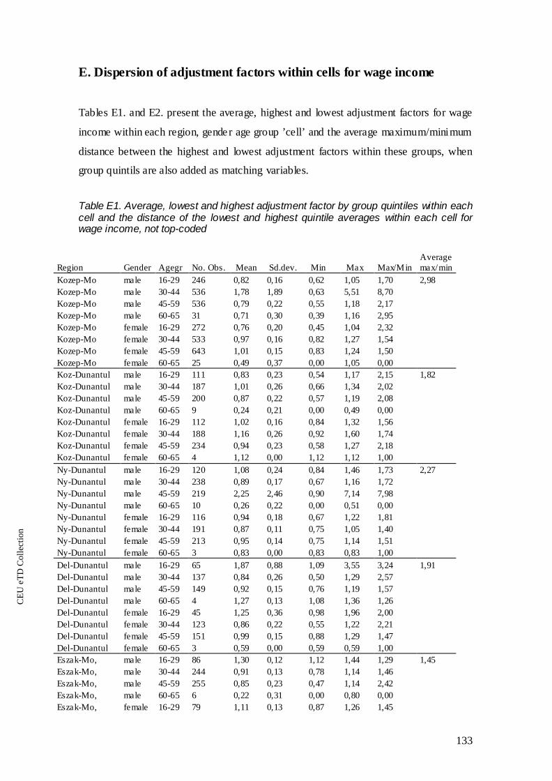
CE

UeT

DC

olle

ctio

n

133

E. Dispersion of adjustment factors within cells for wage income

Tables E1. and E2. present the average, highest and lowest adjustment factors for wage

income within each region, gender age group ’cell’ and the average maximum/minimum

distance between the highest and lowest adjustment factors within these groups, when

group quintils are also added as matching variables.

Table E1. Average, lowest and highest adjustment factor by group quintiles within each cell and the distance of the lowest and highest quintile averages within each cell for wage income, not top-coded

Region Gender Agegr No. Obs. Mean Sd.dev. Min Max Max/Min

Average max/min

Kozep-Mo male 16-29 246 0,82 0,16 0,62 1,05 1,70 2,98 Kozep-Mo male 30-44 536 1,78 1,89 0,63 5,51 8,70 Kozep-Mo male 45-59 536 0,79 0,22 0,55 1,18 2,17 Kozep-Mo male 60-65 31 0,71 0,30 0,39 1,16 2,95 Kozep-Mo female 16-29 272 0,76 0,20 0,45 1,04 2,32 Kozep-Mo female 30-44 533 0,97 0,16 0,82 1,27 1,54 Kozep-Mo female 45-59 643 1,01 0,15 0,83 1,24 1,50 Kozep-Mo female 60-65 25 0,49 0,37 0,00 1,05 0,00 Koz-Dunantul male 16-29 111 0,83 0,23 0,54 1,17 2,15 1,82 Koz-Dunantul male 30-44 187 1,01 0,26 0,66 1,34 2,02 Koz-Dunantul male 45-59 200 0,87 0,22 0,57 1,19 2,08 Koz-Dunantul male 60-65 9 0,24 0,21 0,00 0,49 0,00 Koz-Dunantul female 16-29 112 1,02 0,16 0,84 1,32 1,56 Koz-Dunantul female 30-44 188 1,16 0,26 0,92 1,60 1,74 Koz-Dunantul female 45-59 234 0,94 0,23 0,58 1,27 2,18 Koz-Dunantul female 60-65 4 1,12 0,00 1,12 1,12 1,00 Ny-Dunantul male 16-29 120 1,08 0,24 0,84 1,46 1,73 2,27 Ny-Dunantul male 30-44 238 0,89 0,17 0,67 1,16 1,72 Ny-Dunantul male 45-59 219 2,25 2,46 0,90 7,14 7,98 Ny-Dunantul male 60-65 10 0,26 0,22 0,00 0,51 0,00 Ny-Dunantul female 16-29 116 0,94 0,18 0,67 1,22 1,81 Ny-Dunantul female 30-44 191 0,87 0,11 0,75 1,05 1,40 Ny-Dunantul female 45-59 213 0,95 0,14 0,75 1,14 1,51 Ny-Dunantul female 60-65 3 0,83 0,00 0,83 0,83 1,00 Del-Dunantul male 16-29 65 1,87 0,88 1,09 3,55 3,24 1,91 Del-Dunantul male 30-44 137 0,84 0,26 0,50 1,29 2,57 Del-Dunantul male 45-59 149 0,92 0,15 0,76 1,19 1,57 Del-Dunantul male 60-65 4 1,27 0,13 1,08 1,36 1,26 Del-Dunantul female 16-29 45 1,25 0,36 0,98 1,96 2,00 Del-Dunantul female 30-44 123 0,86 0,22 0,55 1,22 2,21 Del-Dunantul female 45-59 151 0,99 0,15 0,88 1,29 1,47 Del-Dunantul female 60-65 3 0,59 0,00 0,59 0,59 1,00 Eszak-Mo, male 16-29 86 1,30 0,12 1,12 1,44 1,29 1,45 Eszak-Mo, male 30-44 244 0,91 0,13 0,78 1,14 1,46 Eszak-Mo, male 45-59 255 0,85 0,23 0,47 1,14 2,42 Eszak-Mo, male 60-65 6 0,22 0,31 0,00 0,80 0,00 Eszak-Mo, female 16-29 79 1,11 0,13 0,87 1,26 1,45

CE

UeT

DC

olle

ctio

n

134

Eszak-Mo, female 30-44 222 1,03 0,10 0,92 1,16 1,27 Eszak-Mo, female 45-59 249 1,00 0,09 0,92 1,18 1,27 Eszak-Mo, female 60-65 3 1,05 0,00 1,05 1,05 1,00 E-Alfo ld male 16-29 105 1,04 0,04 0,96 1,09 1,13 2,53 E-Alfo ld male 30-44 252 1,47 1,01 0,89 3,46 3,91 E-Alfo ld male 45-59 200 0,97 0,15 0,83 1,23 1,48 E-Alfo ld male 60-65 6 1,19 0,50 0,42 1,99 4,69 E-Alfo ld female 16-29 119 1,28 0,13 1,11 1,45 1,31 E-Alfo ld female 30-44 249 1,00 0,09 0,93 1,18 1,28 E-Alfo ld female 45-59 249 0,93 0,11 0,79 1,14 1,44 E-Alfo ld female 60-65 6 1,07 0,75 0,40 2,00 5,01 D-Alfold male 16-29 106 0,97 0,23 0,80 1,40 1,75 2,63 D-Alfold male 30-44 265 0,83 0,12 0,72 1,02 1,43 D-Alfold male 45-59 261 0,91 0,12 0,75 1,06 1,42 D-Alfold male 60-65 7 0,58 0,35 0,24 1,01 4,26 D-Alfold female 16-29 119 1,00 0,14 0,89 1,27 1,43 D-Alfold female 30-44 255 1,00 0,15 0,84 1,18 1,40 D-Alfold female 45-59 228 0,92 0,16 0,79 1,23 1,56 D-Alfold female 60-65 7 0,53 0,39 0,14 1,09 7,84

CE

UeT

DC

olle

ctio

n

135

Table E2. Average, lowest and highest adjustment factor by group quintiles within each cell and the distance of the lowest and highest quintile averages within each cell for wage income, top-coded

Region Gender Agegr No. Obs. Mean Sd.dev. Min Max Max/Min

Average max/min

Kozep-Mo male 16-29 246 0,81 0,15 0,62 1,00 1,62 1,53 Kozep-Mo male 30-44 536 0,83 0,16 0,63 1,00 1,58 Kozep-Mo male 45-59 536 0,76 0,16 0,55 1,00 1,83 Kozep-Mo male 60-65 31 0,67 0,23 0,39 1,00 2,54 Kozep-Mo female 16-29 272 0,75 0,19 0,45 1,00 2,22 Kozep-Mo female 30-44 533 0,91 0,07 0,82 1,00 1,21 Kozep-Mo female 45-59 643 0,94 0,06 0,83 1,00 1,21 Kozep-Mo female 60-65 25 0,48 0,35 0,00 1,00 0,00 Koz-Dunantul male 16-29 111 0,79 0,18 0,54 1,00 1,84 1,26 Koz-Dunantul male 30-44 187 0,88 0,13 0,66 1,00 1,51 Koz-Dunantul male 45-59 200 0,84 0,17 0,57 1,00 1,74 Koz-Dunantul male 60-65 9 0,24 0,21 0,00 0,49 0,00 Koz-Dunantul female 16-29 112 0,95 0,06 0,84 1,00 1,19 Koz-Dunantul female 30-44 188 0,98 0,03 0,92 1,00 1,09 Koz-Dunantul female 45-59 234 0,87 0,16 0,58 1,00 1,72 Koz-Dunantul female 60-65 4 1,00 0,00 1,00 1,00 1,00 Ny-Dunantul male 16-29 120 0,93 0,08 0,84 1,00 1,19 1,12 Ny-Dunantul male 30-44 238 0,86 0,13 0,67 1,00 1,48 Ny-Dunantul male 45-59 219 0,96 0,05 0,90 1,00 1,12 Ny-Dunantul male 60-65 10 0,26 0,22 0,00 0,51 0,00 Ny-Dunantul female 16-29 116 0,89 0,12 0,67 1,00 1,48 Ny-Dunantul female 30-44 191 0,86 0,10 0,75 1,00 1,33 Ny-Dunantul female 45-59 213 0,92 0,10 0,75 1,00 1,33 Ny-Dunantul female 60-65 3 0,83 0,00 0,83 0,83 1,00 Del-Dunantul male 16-29 65 1,00 0,00 1,00 1,00 1,00 1,28 Del-Dunantul male 30-44 137 0,78 0,17 0,50 1,00 1,99 Del-Dunantul male 45-59 149 0,88 0,09 0,76 1,00 1,32 Del-Dunantul male 60-65 4 1,00 0,00 1,00 1,00 1,00 Del-Dunantul female 16-29 45 1,00 0,01 0,98 1,00 1,02 Del-Dunantul female 30-44 123 0,81 0,15 0,55 1,00 1,80 Del-Dunantul female 45-59 151 0,93 0,04 0,88 1,00 1,13 Del-Dunantul female 60-65 3 0,59 0,00 0,59 0,59 1,00 Eszak-Mo, male 16-29 86 1,00 0,00 1,00 1,00 1,00 1,09 Eszak-Mo, male 30-44 244 0,88 0,09 0,78 1,00 1,28 Eszak-Mo, male 45-59 255 0,82 0,20 0,47 1,00 2,11 Eszak-Mo, male 60-65 6 0,22 0,31 0,00 0,80 0,00 Eszak-Mo, female 16-29 79 0,97 0,05 0,87 1,00 1,15 Eszak-Mo, female 30-44 222 0,98 0,03 0,92 1,00 1,09 Eszak-Mo, female 45-59 249 0,96 0,03 0,92 1,00 1,08 Eszak-Mo, female 60-65 3 1,00 0,00 1,00 1,00 1,00 E-Alfo ld male 16-29 105 0,99 0,01 0,96 1,00 1,04 1,45 E-Alfo ld male 30-44 252 0,95 0,05 0,89 1,00 1,13 E-Alfo ld male 45-59 200 0,92 0,07 0,83 1,00 1,20 E-Alfo ld male 60-65 6 0,90 0,24 0,42 1,00 2,36 E-Alfo ld female 16-29 119 1,00 0,00 1,00 1,00 1,00 E-Alfo ld female 30-44 249 0,96 0,03 0,93 1,00 1,08 E-Alfo ld female 45-59 249 0,90 0,07 0,79 1,00 1,27 E-Alfo ld female 60-65 6 0,73 0,27 0,40 1,00 2,50

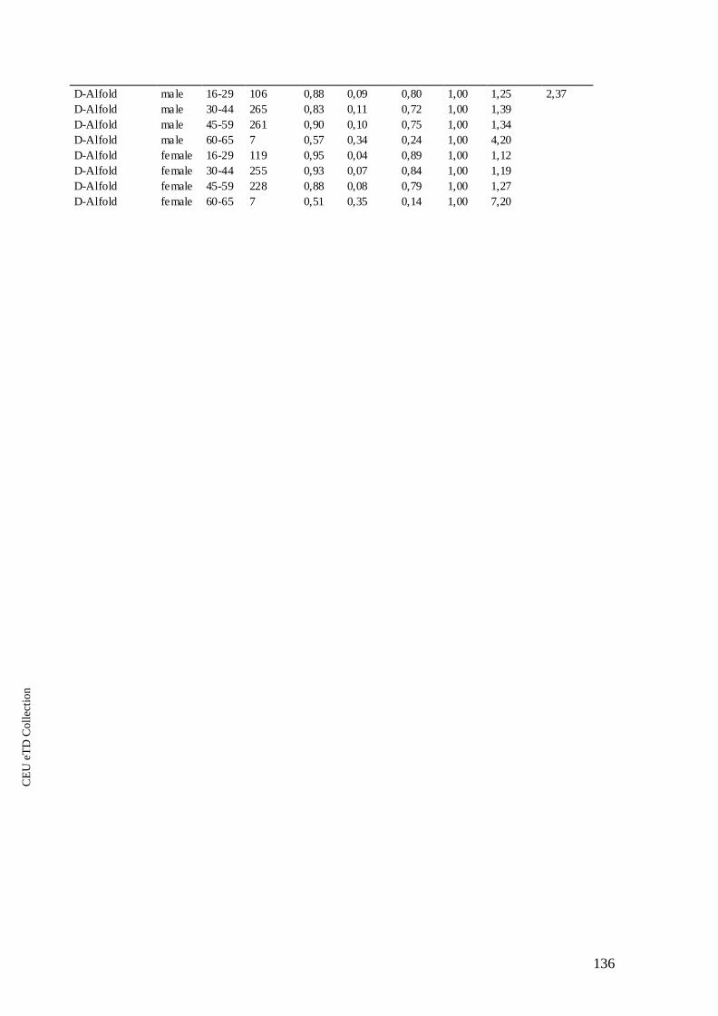
CE

UeT

DC

olle

ctio

n

136

D-Alfold male 16-29 106 0,88 0,09 0,80 1,00 1,25 2,37 D-Alfold male 30-44 265 0,83 0,11 0,72 1,00 1,39 D-Alfold male 45-59 261 0,90 0,10 0,75 1,00 1,34 D-Alfold male 60-65 7 0,57 0,34 0,24 1,00 4,20 D-Alfold female 16-29 119 0,95 0,04 0,89 1,00 1,12 D-Alfold female 30-44 255 0,93 0,07 0,84 1,00 1,19 D-Alfold female 45-59 228 0,88 0,08 0,79 1,00 1,27 D-Alfold female 60-65 7 0,51 0,35 0,14 1,00 7,20