essays on corruption - lsu digital commons
TRANSCRIPT
Louisiana State UniversityLSU Digital Commons
LSU Doctoral Dissertations Graduate School
2015
Essays on CorruptionChandan Kumar JhaLouisiana State University and Agricultural and Mechanical College, [email protected]
Follow this and additional works at: https://digitalcommons.lsu.edu/gradschool_dissertations
Part of the Economics Commons
This Dissertation is brought to you for free and open access by the Graduate School at LSU Digital Commons. It has been accepted for inclusion inLSU Doctoral Dissertations by an authorized graduate school editor of LSU Digital Commons. For more information, please [email protected].
Recommended CitationJha, Chandan Kumar, "Essays on Corruption" (2015). LSU Doctoral Dissertations. 2669.https://digitalcommons.lsu.edu/gradschool_dissertations/2669
ESSAYS ON CORRUPTION
A Dissertation
Submitted to the Graduate Faculty of theLouisiana State University and
Agricultural and Mechanical Collegein partial fulfillment of the
requirements for the degree ofDoctor of Philosophy
in
The Department of Economics
byChandan Kumar Jha
M.A., Gokhale Institute of Politics and Economics, 2010M.S., Louisiana State University, 2012
August 2015
Dedicated to my grandparents Kashikant and Tara Jhaand
my parents Sudhir and Durga Jha.
ii
Acknowledgments
First, I would like to thank all my family members for showing immense faith in me
and for always being supportive and encouraging. Without their sacrifices, this dissertation
would never have come into existence.
I am greatly indebted to my advisor Sudipta Sarangi for his inspiration and the patience
that he has shown during my doctoral studies. I am very grateful to my advisors Douglas
McMillin, Areendam Chanda, and Louis-Philippe Beland, who have always been supportive
and kept their office doors open for me to discuss my papers and provided valuable feedback
and suggestions to improve this dissertation. I would also like to thank Jacqueline Moffitt
for agreeing to be on my dissertation committee.
Finally, I would also like to thank the members of my village who have always been
encouraging and have shown tremendous faith in me, and my friends for their love and
unconditional support that helped me overcome numerous challenges due the course my
doctoral studies.
iii
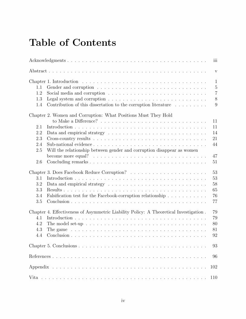
Table of Contents
Acknowledgments . . . . . . . . . . . . . . . . . . . . . . . . . . . . . . . . . . . . . . iii
Abstract . . . . . . . . . . . . . . . . . . . . . . . . . . . . . . . . . . . . . . . . . . . v
Chapter 1. Introduction . . . . . . . . . . . . . . . . . . . . . . . . . . . . . . . . . . 11.1 Gender and corruption . . . . . . . . . . . . . . . . . . . . . . . . . . . . . . 51.2 Social media and corruption . . . . . . . . . . . . . . . . . . . . . . . . . . . 71.3 Legal system and corruption . . . . . . . . . . . . . . . . . . . . . . . . . . . 81.4 Contribution of this dissertation to the corruption literature . . . . . . . . . 9
Chapter 2. Women and Corruption: What Positions Must They Holdto Make a Difference? . . . . . . . . . . . . . . . . . . . . . . . . . . . . . 11
2.1 Introduction . . . . . . . . . . . . . . . . . . . . . . . . . . . . . . . . . . . . 112.2 Data and empirical strategy . . . . . . . . . . . . . . . . . . . . . . . . . . . 142.3 Cross-country results . . . . . . . . . . . . . . . . . . . . . . . . . . . . . . . 212.4 Sub-national evidence . . . . . . . . . . . . . . . . . . . . . . . . . . . . . . . 442.5 Will the relationship between gender and corruption disappear as women
become more equal? . . . . . . . . . . . . . . . . . . . . . . . . . . . . . . . 472.6 Concluding remarks . . . . . . . . . . . . . . . . . . . . . . . . . . . . . . . . 51
Chapter 3. Does Facebook Reduce Corruption? . . . . . . . . . . . . . . . . . . . . . 533.1 Introduction . . . . . . . . . . . . . . . . . . . . . . . . . . . . . . . . . . . . 533.2 Data and empirical strategy . . . . . . . . . . . . . . . . . . . . . . . . . . . 583.3 Results . . . . . . . . . . . . . . . . . . . . . . . . . . . . . . . . . . . . . . . 653.4 Falsification test for the Facebook-corruption relationship . . . . . . . . . . . 763.5 Conclusion . . . . . . . . . . . . . . . . . . . . . . . . . . . . . . . . . . . . . 77
Chapter 4. Effectiveness of Asymmetric Liability Policy: A Theoretical Investigation . 794.1 Introduction . . . . . . . . . . . . . . . . . . . . . . . . . . . . . . . . . . . . 794.2 The model set-up . . . . . . . . . . . . . . . . . . . . . . . . . . . . . . . . . 804.3 The game . . . . . . . . . . . . . . . . . . . . . . . . . . . . . . . . . . . . . 814.4 Conclusion . . . . . . . . . . . . . . . . . . . . . . . . . . . . . . . . . . . . . 92
Chapter 5. Conclusions . . . . . . . . . . . . . . . . . . . . . . . . . . . . . . . . . . . 93
References . . . . . . . . . . . . . . . . . . . . . . . . . . . . . . . . . . . . . . . . . . 96
Appendix . . . . . . . . . . . . . . . . . . . . . . . . . . . . . . . . . . . . . . . . . . 102
Vita . . . . . . . . . . . . . . . . . . . . . . . . . . . . . . . . . . . . . . . . . . . . . 110
iv
Abstract
Corruption is a global concern and requires attention because of its detrimental effects
on economic growth and development. This dissertation includes three different essays that
identify some of the instruments that can be used to fight corruption. The first essay in-
vestigates whether women’s presence in economic and political arenas can have a significant
impact on corruption. It finds evidence that while women’s presence in parliament does
reduce corruption other measures of female participation in economic activities are shown to
have no effect. The second essay shows that internet and Facebook have an adverse effect on
corruption. Finally, in a theoretical analysis the concluding essay finds that an asymmetric
liability policy may not be effective in reducing bribery. A modification in the asymmetric
liability policy is suggested and is shown to be more effective.
v
Chapter 1. Introduction
Just as it is not possible not to taste honey or poison placed on thesurface of the tongue, even so it is not possible for one dealing withthe money of the king not to taste the money in however small aquantity. Just as fish moving inside water cannot be known whendrinking water, even so officers appointed for carrying out works can-not be known when appropriating money. It is possible to know eventhe path of birds flying in the sky, but not the ways of officers movingwith their intentions concealed.
Kautiliya’s Arthasastra (Kangle, 2000, p-91)
Corruption is an age-old problem and has been present in various forms such as bribery,
extortion, cronyism, nepotism and embezzlement since the beginning of the civilization. In
simplest terms, corruption is any act that is intended to wrongfully increase the private gain
of an individual who is able to do so because of the power granted to him by the public or an
institution democratically elected by the public. In most of the cases, detecting corruption
is very difficult, more so when the act of corruption or bribery is mutually beneficial. For
instance, imagine a scenario where a person or a firm makes hidden extra payments to an
official in exchange for a service or a license that the former is not entitled to. In this
case, neither the bribe payer nor the bribe taker has an incentive to report bribery and
therefore it’s very difficult, if not impossible, to detect the bribery and prove it in the court
of law. Such acts of bribery are known as collusive bribery where both the involved parties
gain undue advantages from the corrupt contract. Although an act of extortionary bribe
or harassment bribe involves a victim–the bribe giver who is forced to pay a bribe in order
to receive the services he/she is entitled to–establishing even such acts of bribery is often
difficult since the victim has little incentives to report the bribe not only because there is a
moral dilemma involved, but also because in many countries the bribe givers are also subject
to legal sanctions. It is because of this very nature of corruption that it is very difficult to
fight corruption.
1
Though it is difficult to measure actual corruption in a country, the World Bank and
Transparency International publish corruption perception indices – the Control of Corruption
Index (CCI) and Corruption Perception Index (CPI) respectively, for a large number of
countries of the world, which reflect the perception of corruption in these countries. The
CCI takes values in the range of -−2.5 to 2.5, and the CPI takes values in the range of 0
to 10: A higher index in both the indices implies a lower corruption. Not a single country
in the world is entirely free from corruption as indicated by these indices. While a large
proportion of countries has a very low score on these indices, none of the countries scores a
perfect. For example, in 2011, New Zealand had the highest CPI, 9.46 out of the maximum
possible 10 (least corrupt), while Denmark had the highest score in the CCI, 2.42 out of the
maximum possible 2.5 (least corrupt). Somalia had the lowest scores, a CPI of 0.98 (the
lowest possible score is 0), and a CCI of -1.72 (-2.5 is the lowest possible score).1
Figure 1.1: Income and Corruption
1 For details on how these indices are constructed, please refer to the data section of Chapter 2.
2
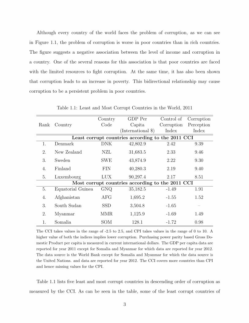
Although every country of the world faces the problem of corruption, as we can see
in Figure 1.1, the problem of corruption is worse in poor countries than in rich countries.
The figure suggests a negative association between the level of income and corruption in
a country. One of the several reasons for this association is that poor countries are faced
with the limited resources to fight corruption. At the same time, it has also been shown
that corruption leads to an increase in poverty. This bidirectional relationship may cause
corruption to be a persistent problem in poor countries.
Table 1.1: Least and Most Corrupt Countries in the World, 2011
Country GDP Per Control of CorruptionRank Country Code Capita Corruption Perception
(International $) Index Index
Least corrupt countries according to the 2011 CCI1. Denmark DNK 42,802.9 2.42 9.39
2. New Zealand NZL 31,683.5 2.33 9.46
3. Sweden SWE 43,874.9 2.22 9.30
4. Finland FIN 40,280.3 2.19 9.40
5. Luxembourg LUX 90,297.4 2.17 8.51Most corrupt countries according to the 2011 CCI
5. Equatorial Guinea GNQ 35,182.5 -1.49 1.91
4. Afghanistan AFG 1,695.2 -1.55 1.52
3. South Sudan SSD 3,504.8 -1.65 –
2. Myanmar MMR 1,125.9 -1.69 1.49
1. Somalia SOM 128.1 -1.72 0.98
The CCI takes values in the range of -2.5 to 2.5, and CPI takes values in the range of 0 to 10. A
higher value of both the indices implies lower corruption. Purchasing power parity based Gross Do-
mestic Product per capita is measured in current international dollars. The GDP per capita data are
reported for year 2011 except for Somalia and Myanmar for which data are reported for year 2012.
The data source is the World Bank except for Somalia and Myanmar for which the data source is
the United Nations. and data are reported for year 2012. The CCI covers more countries than CPI
and hence missing values for the CPI.
Table 1.1 lists five least and most corrupt countries in descending order of corruption as
measured by the CCI. As can be seen in the table, some of the least corrupt countries of
3
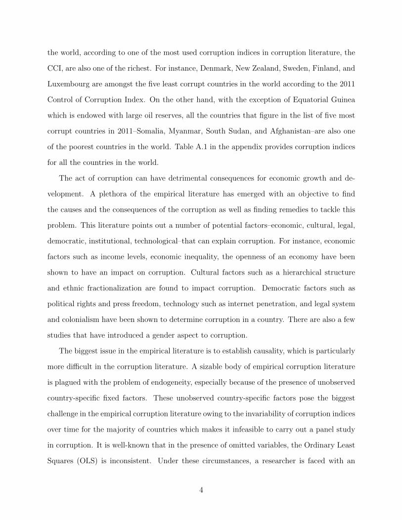
the world, according to one of the most used corruption indices in corruption literature, the
CCI, are also one of the richest. For instance, Denmark, New Zealand, Sweden, Finland, and
Luxembourg are amongst the five least corrupt countries in the world according to the 2011
Control of Corruption Index. On the other hand, with the exception of Equatorial Guinea
which is endowed with large oil reserves, all the countries that figure in the list of five most
corrupt countries in 2011–Somalia, Myanmar, South Sudan, and Afghanistan–are also one
of the poorest countries in the world. Table A.1 in the appendix provides corruption indices
for all the countries in the world.
The act of corruption can have detrimental consequences for economic growth and de-
velopment. A plethora of the empirical literature has emerged with an objective to find
the causes and the consequences of the corruption as well as finding remedies to tackle this
problem. This literature points out a number of potential factors–economic, cultural, legal,
democratic, institutional, technological–that can explain corruption. For instance, economic
factors such as income levels, economic inequality, the openness of an economy have been
shown to have an impact on corruption. Cultural factors such as a hierarchical structure
and ethnic fractionalization are found to impact corruption. Democratic factors such as
political rights and press freedom, technology such as internet penetration, and legal system
and colonialism have been shown to determine corruption in a country. There are also a few
studies that have introduced a gender aspect to corruption.
The biggest issue in the empirical literature is to establish causality, which is particularly
more difficult in the corruption literature. A sizable body of empirical corruption literature
is plagued with the problem of endogeneity, especially because of the presence of unobserved
country-specific fixed factors. These unobserved country-specific factors pose the biggest
challenge in the empirical corruption literature owing to the invariability of corruption indices
over time for the majority of countries which makes it infeasible to carry out a panel study
in corruption. It is well-known that in the presence of omitted variables, the Ordinary Least
Squares (OLS) is inconsistent. Under these circumstances, a researcher is faced with an
4
enormous task of identifying appropriate instruments that are both valid and strong. A
valid instrument is correlated with the endogenous variable and does not have any impact
on the dependent variable (in this case, corruption) except via its effect on the variable that
is being instrumented. The recent literature, however, has developed methods that can be
used to make robust inferences when the instruments, though valid, are not strong (Moreira,
2003; Kleibergen, 2002). This dissertation deals with the issue of causality by identifying
appropriate instruments and uses the conditional likelihood ratio approach to draw robust
inferences whenever the instruments are not strong.
This dissertation deals with three different aspects of corruption. The second chapter
of this dissertation revisits the gender aspect of corruption that claims that (a) there is a
negative association between women’s share in the labor force and corruption, and (b) there
is a negative association between women’s share in parliament and corruption. Revisiting
this relationship is important because the issue of causality has not been resolved, and
there is no conclusive evidence of a causal association between women’s presence in the
spheres mentioned above and corruption. The third chapter proposes a novel instrument
to fight corruption and shows that the social media can be used as a tool to fight against
corruption. The fourth chapter goes into the legal aspects of corruption and presents a
theoretical investigation of different legal systems on corruption. The chapter ends with
proposing certain measures to fight corruption effectively. Finally, conclusions are drawn in
Chapter 5.
1.1 Gender and corruption
In many economic settings women have been found to behave differently from men and have
even been shown to be less selfish than men (see Eckel and Grossman, 1998 and references
therein). Based on this finding a strand of literature has explored the role of gender in
determining corruption, and has investigated whether women in the labor force can impact
5
corruption (Swamy et al., 2001) and whether women in the parliament and government can
have a negative impact on corruption (Swamy et al., 2001; Dollar et al., 2001). These studies
find that gender representation in the labor force and government is negatively associated
with corruption. The later studies, however, questioned these results and argued that this
relationship is not causal. These studies argued that it is the omission of some of the relevant
factors such as liberal democracy and women’s exposure to bribe taking activities from the
model that causes a spurious relationship between gender and corruption (Sung, 2003; Goetz,
2007). In an experimental study, women are even found to be more opportunistic when there
is a possibility to break a corrupt contract (Frank et al., 2011).
The evidence on the corruptibility of women, therefore, is essentially mixed giving rise to
the need for determining whether the observed relationship between gender and corruption is
causal. The second chapter of this thesis deals with the problem of endogeneity and address
the causality issues by using instruments for women’s presence in economic and political
activities. The chapter explores the historical and linguistic factors that can explain modern
gender inequality and hence prove to be good instruments for women’s participation in
economic and political activities. These instruments, however, are not always strong. This
issue is overcome by using newly developed methods that allow for robust inferences in the
presence of weak instruments.
Apart from investigating the impact of gender representation in the labor force and in
parliament on corruption, this chapter also introduces two new measures of women’s presence
in economic activities, that is, women’s share in decision making positions and women’s share
in clerical positions, and looks at their impact on corruption. This exercise is carried out with
an objective to identify the specific roles in which women can affect corruption and to gain
insights on the interaction between women’s presence in economic and political activities
on corruption. The chapter also discusses the potential channels through which women are
able to have an impact on corruption. Finally, the chapter also provides evidence regarding
a much-cited hypothesis which argues that the observed association between gender and
6
corruption will vanish over times as this association may have actually been driven by the
gender differences in social status or because of the possibility that women may have limited
access to networks of corruption (Swamy et al., 2001; Goetz, 2007).
1.2 Social media and corruption
The advent of the information and communication technology (ICT) has changed our lives
drastically and has expanded our political, social and economic freedom. ICT provides multi-
way forms of communication and, therefore, establishes a superiority over the print media
and broadcast media which provide only one-way communication and has been subject to
censure and control by the authoritarian regimes. These regimes have censored and controlled
the information that can be accessed by the public. Often the cases of corruption, human
rights violations and police brutality have been taboo subjects for citizens and have been
censored in several countries such as China, Malaysia, and Iran. The invention and spread of
internet challenged the monopoly of the governments in authoritarian regimes on the sources
of information and resulted in this information to be available to the public. Recently the
use of social media has augmented these effects. By providing multi-way communication, the
social media and internet make it difficult for the authoritarian regimes to censor information.
The influence of the internet in undemocratic societies has been so profound that it
has given rise to the concept of “Dictator’s Dilemma”. The dictator’s dilemma refers to
the trade-off that a dictator has to face – an increased internet penetration allowed by the
dictator increases the risk of overthrow (by providing activists with a platform to organize
resistance against the dictator), and restricting internet availability will hinder economic
growth by cutting the economy off the world, and exchange of ideas (Kedzie, 1997). The
internet and the social media promote transparency, communication of information, sharing
of ideas, and help mobilize support for a social cause. The social media were extensively
used in the Middle-East uprisings and have been recognized to play an instrumental role in
7
the success of uprisings in Egypt, Libya, Tunisia, and Yemen (Howard and Hussain, 2011;
Dalacoura, 2012). In words of an Egyptian protester - “We use Facebook to schedule the
protests, Twitter to coordinate, and YouTube to tell the world”.
Based on above facts, the third chapter of this thesis explores the possibility that increas-
ing use of social media may have a negative impact on corruption. Social media platforms
have extensively been used to mobilize support and organize protests against corrupt ac-
tivities in India and have helped these anti-corruption movements to be successful (Jha,
2014). In addition, the chapter also revisits the relationship between internet penetration
and corruption.
1.3 Legal system and corruption
Countries differ in their legal systems and their laws against bribery. While certain acts can
be termed as bribery and, therefore, may be subject to legal punishment in some countries,
these acts may be perfectly acceptable in other countries. The legal system also differs across
countries in their treatment of the bribe giver and bribe taker. For instance, in a number of
countries such as China, Japan, and Russia the legal punishment for bribe givers is milder
than that for the bribe takers. On the other hand, other countries such as Germany, India,
the United Kingdom, and the United States treat bribe-giver as well as bribe-taker equally
culpable. A legal system that treats both the bribe giver and the bribe taker equally culpable
is known as the symmetric liability regime. The asymmetric liability regime, on the other
hand, is lenient on the bribe giver and severely punishes the bribe taker.
Basu (2011) proposed that India should implement asymmetric liability for a class of
bribes known as harassment bribes in which a person is forced to pay a bribe to avail the
services he/she is entitled to. He argued that doing so will result in a decrease in bribery
since the bribe giver will have a greater incentive to report bribery given that she will not be
subject to legal sanctions anymore. This proposal, however, was not free from criticisms and
8
it was argued that moving from a symmetric liability regime to an asymmetric liability regime
may not necessarily lead to a decrease in bribery, and may even increase it (Dreze, 2011).
The proposal was also criticized on the grounds that it may promote unethical behavior and
may make bribe giving an acceptable norm.
The fourth chapter of this thesis evaluates the merits of an asymmetric liability policy
and theoretically investigates whether this policy has a potential to reduce bribery and
whether it requires additional policy modifications to incentivize the bribe giver to report
bribe incidents. The chapter also suggests some modifications in the asymmetric liability
policy in order to produce desired outcomes and mitigate the problem of morality which
such policies might bring in.
1.4 Contribution of this dissertation to the corruption literature
The main contributions of this dissertation in the literature studying corruption include, but
is not limited to, the following
• Establishing causality in gender-corruption literature: This dissertation is the
first in gender-corruption literature to use an instrumental variable (IV) analysis and
establishes causality.
• Women’s role in determining corruption: Chapter 2 of this dissertation identifies
the precise role in which women are able to reduce corruption. The chapter also pro-
vides evidence that, contrary to the hypothesis of the previous studies, the relationship
between gender and corruption is unlikely to vanish as women get similar in status as
men.
• Social media and corruption: Chapter 3 of this dissertation is the first quanti-
tatively comprehensive study that provides evidence to support the hypothesis that
social media can be used as a tool against corruption. The chapter also uses a dif-
9

ferent instrument to show that the relationship between the internet penetration and
corruption shown by earlier studies is robust.
• Legal system and corruption: The dissertation also develops a theoretical model
to show that legal system matters for corruption and changes in legal systems have the
potential to reduce corruption in many, especially developing, countries of the world.
The dissertation also cautions against a blind replication of legal regimes by showing
that the impact of a legal regime on bribery depends on several other factors and that
these must be taken into account while contemplating a change in legal policies.
10
Chapter 2. Women and Corruption: WhatPositions Must They Holdto Make a Difference?
2.1 Introduction
Corruption remains an important issue both in poor countries and advanced economies be-
cause of its negative impact on economic outcomes such as investment, economic growth,
and per capita income.1 Little over a decade ago a gender dimension was added to this topic
through two classic papers by Swamy et al. (2001) and Dollar et al. (2001), both drawing
on the notion that women behave differently from men in many economic circumstances.2
The latter study found a negative correlation between women’s presence in parliament and
corruption, while the former reported lower corruption to be correlated with both women’s
presence in the labor force as well as in parliament using cross-country analysis. Subse-
quently, however, a number of studies have voiced concerns that this observed negative
association between gender and corruption was not causal and driven by the omission of
other factors that might be correlated with women’s participation and/or corruption in a
country. In this chapter, we address the concerns raised in this literature by first looking for
a causal relationship between gender and corruption using instrumental variable (IV) anal-
ysis and second by taking a more nuanced approach to this problem by identifying different
economic roles women can take vis-a-vis corruption and investigating the impact of each on
corruption.
We start by pointing out that the term “labor force” which has been found to be neg-
atively correlated with corruption in earlier studies is a very broad measure and does not
1 For instance, a higher level of corruption is associated with lower levels of GDP per capita (World Bank,2001); lower rates of investment and economic growth (Mauro, 1995); high inequality and poverty (Guptaet al., 2002).
2 A number of studies support this hypothesis (see Eckel and Grossman (1998) and references therein).
11
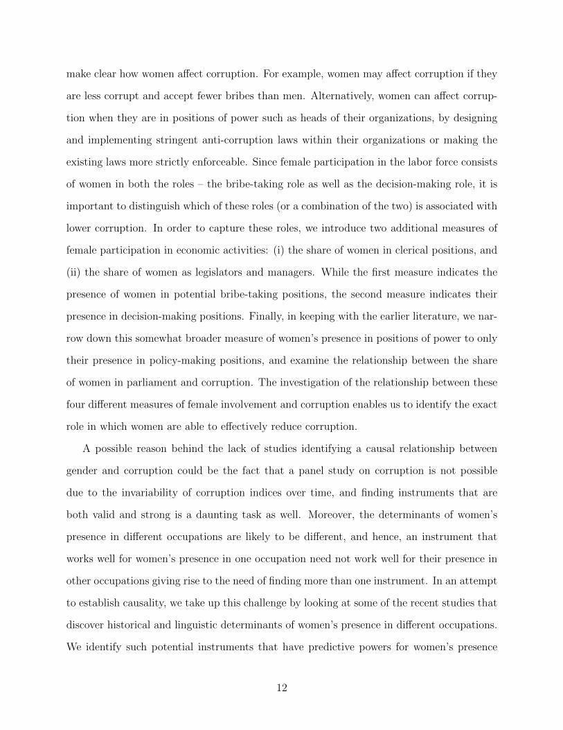
make clear how women affect corruption. For example, women may affect corruption if they
are less corrupt and accept fewer bribes than men. Alternatively, women can affect corrup-
tion when they are in positions of power such as heads of their organizations, by designing
and implementing stringent anti-corruption laws within their organizations or making the
existing laws more strictly enforceable. Since female participation in the labor force consists
of women in both the roles – the bribe-taking role as well as the decision-making role, it is
important to distinguish which of these roles (or a combination of the two) is associated with
lower corruption. In order to capture these roles, we introduce two additional measures of
female participation in economic activities: (i) the share of women in clerical positions, and
(ii) the share of women as legislators and managers. While the first measure indicates the
presence of women in potential bribe-taking positions, the second measure indicates their
presence in decision-making positions. Finally, in keeping with the earlier literature, we nar-
row down this somewhat broader measure of women’s presence in positions of power to only
their presence in policy-making positions, and examine the relationship between the share
of women in parliament and corruption. The investigation of the relationship between these
four different measures of female involvement and corruption enables us to identify the exact
role in which women are able to effectively reduce corruption.
A possible reason behind the lack of studies identifying a causal relationship between
gender and corruption could be the fact that a panel study on corruption is not possible
due to the invariability of corruption indices over time, and finding instruments that are
both valid and strong is a daunting task as well. Moreover, the determinants of women’s
presence in different occupations are likely to be different, and hence, an instrument that
works well for women’s presence in one occupation need not work well for their presence in
other occupations giving rise to the need of finding more than one instrument. In an attempt
to establish causality, we take up this challenge by looking at some of the recent studies that
discover historical and linguistic determinants of women’s presence in different occupations.
We identify such potential instruments that have predictive powers for women’s presence
12
in different positions, yet there is little reason to expect a direct effect of these variables
on corruption. We experiment with multiple instruments to explore the causal relationship
between the share of women in parliament and corruption. While using more than one
instrument for one endogenous variable allows us to check for the validity of our instruments
conditional on at least one of our instruments being valid, our instruments tend to be weak
in some specifications which may lead to invalid inferences. We overcome this possibility
by using the conditional likelihood ratio (CLR) approach developed by Moreira (2003) for
hypothesis testing that provides for the robust inferences in the presence of weak instruments.
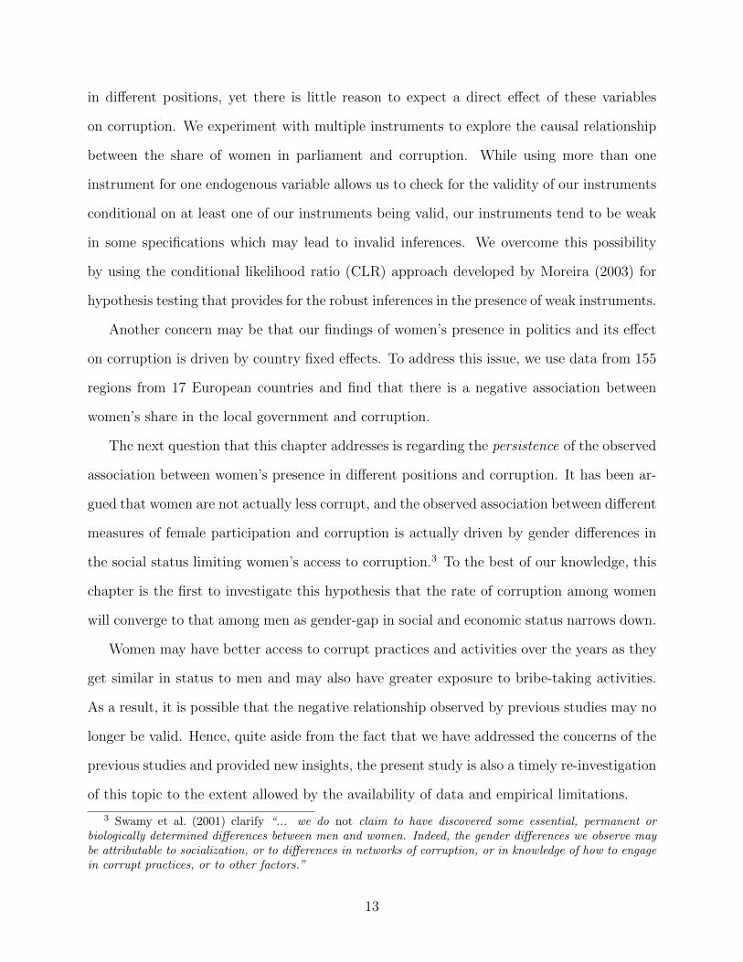
Another concern may be that our findings of women’s presence in politics and its effect
on corruption is driven by country fixed effects. To address this issue, we use data from 155
regions from 17 European countries and find that there is a negative association between
women’s share in the local government and corruption.
The next question that this chapter addresses is regarding the persistence of the observed
association between women’s presence in different positions and corruption. It has been ar-
gued that women are not actually less corrupt, and the observed association between different
measures of female participation and corruption is actually driven by gender differences in
the social status limiting women’s access to corruption.3 To the best of our knowledge, this
chapter is the first to investigate this hypothesis that the rate of corruption among women
will converge to that among men as gender-gap in social and economic status narrows down.
Women may have better access to corrupt practices and activities over the years as they
get similar in status to men and may also have greater exposure to bribe-taking activities.
As a result, it is possible that the negative relationship observed by previous studies may no
longer be valid. Hence, quite aside from the fact that we have addressed the concerns of the
previous studies and provided new insights, the present study is also a timely re-investigation
of this topic to the extent allowed by the availability of data and empirical limitations.
3 Swamy et al. (2001) clarify “... we do not claim to have discovered some essential, permanent orbiologically determined differences between men and women. Indeed, the gender differences we observe maybe attributable to socialization, or to differences in networks of corruption, or in knowledge of how to engagein corrupt practices, or to other factors.”
13
Our main results are as follows. The role in which women have an impact on corruption
is through their presence in politics. Using an IV approach we show that this relationship
is robust and causal. Moreover, our findings hold at both, the national and sub-national,
levels. We also show that the observed negative relationship between female participation
and corruption cannot entirely be explained by gender differences in social status.
The rest of the chapter is organized as follows. In the next section, we discuss our sources
of data and specify empirical strategy as well as establish the validity of our instruments.
Section 2.3 reports cross-country OLS and IV results, and section 2.4 presents sub-national
evidence. We check whether there is an evidence of “corruption convergence in gender” in
section 2.5 and discuss the implications of our findings in section 2.6.
2.2 Data and empirical strategy
2.2.1 Data
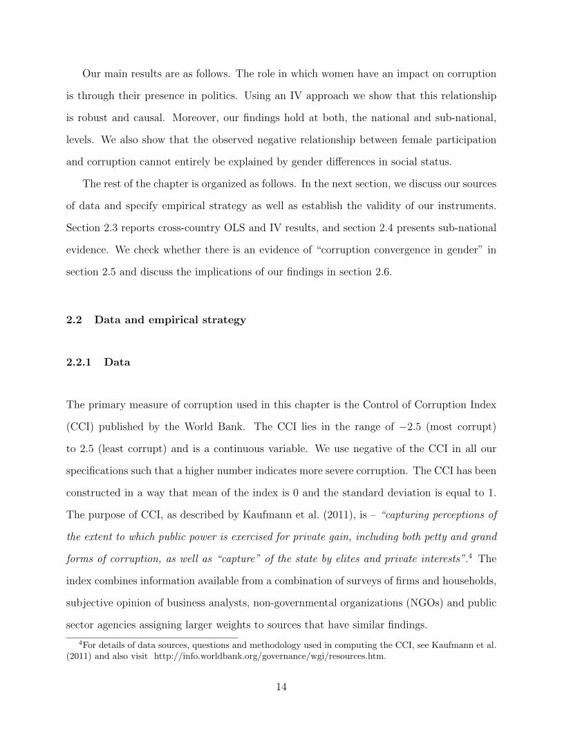
The primary measure of corruption used in this chapter is the Control of Corruption Index
(CCI) published by the World Bank. The CCI lies in the range of −2.5 (most corrupt)
to 2.5 (least corrupt) and is a continuous variable. We use negative of the CCI in all our
specifications such that a higher number indicates more severe corruption. The CCI has been
constructed in a way that mean of the index is 0 and the standard deviation is equal to 1.
The purpose of CCI, as described by Kaufmann et al. (2011), is – “capturing perceptions of
the extent to which public power is exercised for private gain, including both petty and grand
forms of corruption, as well as “capture” of the state by elites and private interests”.4 The
index combines information available from a combination of surveys of firms and households,
subjective opinion of business analysts, non-governmental organizations (NGOs) and public
sector agencies assigning larger weights to sources that have similar findings.
4For details of data sources, questions and methodology used in computing the CCI, see Kaufmann et al.(2011) and also visit http://info.worldbank.org/governance/wgi/resources.htm.
14
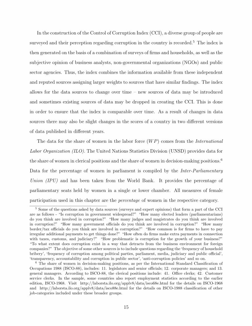
In the construction of the Control of Corruption Index (CCI), a diverse group of people are
surveyed and their perception regarding corruption in the country is recorded.5 The index is
then generated on the basis of a combination of surveys of firms and households, as well as the
subjective opinion of business analysts, non-governmental organizations (NGOs) and public
sector agencies. Thus, the index combines the information available from these independent
and reputed sources assigning larger weights to sources that have similar findings. The index
allows for the data sources to change over time – new sources of data may be introduced
and sometimes existing sources of data may be dropped in creating the CCI. This is done
in order to ensure that the index is comparable over time. As a result of changes in data
sources there may also be slight changes in the scores of a country in two different versions
of data published in different years.
The data for the share of women in the labor force (WP ) comes from the International
Labor Organization (ILO). The United Nations Statistics Division (UNSD) provides data for
the share of women in clerical positions and the share of women in decision-making positions.6
Data for the percentage of women in parliament is compiled by the Inter-Parliamentary
Union (IPU) and has been taken from the World Bank. It provides the percentage of
parliamentary seats held by women in a single or lower chamber. All measures of female
participation used in this chapter are the percentage of women in the respective category.
5 Some of the questions asked by data sources (surveys and expert opinions) that form a part of the CCIare as follows - “Is corruption in government widespread?” “How many elected leaders (parliamentarians)do you think are involved in corruption?” “How many judges and magistrates do you think are involvedin corruption?” “How many government officials do you think are involved in corruption?” “How manyborder/tax officials do you think are involved in corruption?” “How common is for firms to have to payirregular additional payments to get things done?” “How often do firms make extra payments in connectionwith taxes, customs, and judiciary?” “How problematic is corruption for the growth of your business?”“To what extent does corruption exist in a way that detracts from the business environment for foreigncompanies?” The objective of some other sources is to include questions regarding the ‘frequency of householdbribery’, ‘frequency of corruption among political parties, parliament, media, judiciary and public official’,‘transparency, accountability and corruption in public sector’, ‘anti-corruption policies’ and so on.
6 The share of women in decision-making positions, as per the International Standard Classification ofOccupations 1988 (ISCO-88), includes: 11. legislators and senior officials; 12. corporate managers; and 13.general managers. According to ISCO-88, the clerical positions include: 41. Office clerks; 42. Customerservice clerks. In the sample, some countries also report employment statistics according to the earlieredition, ISCO-1968. Visit http://laborsta.ilo.org/applv8/data/isco68e.html for the details on ISCO-1968and http://laborsta.ilo.org/applv8/data/isco88e.html for the details on ISCO-1988 classification of otherjob-categories included under these broader groups.
15
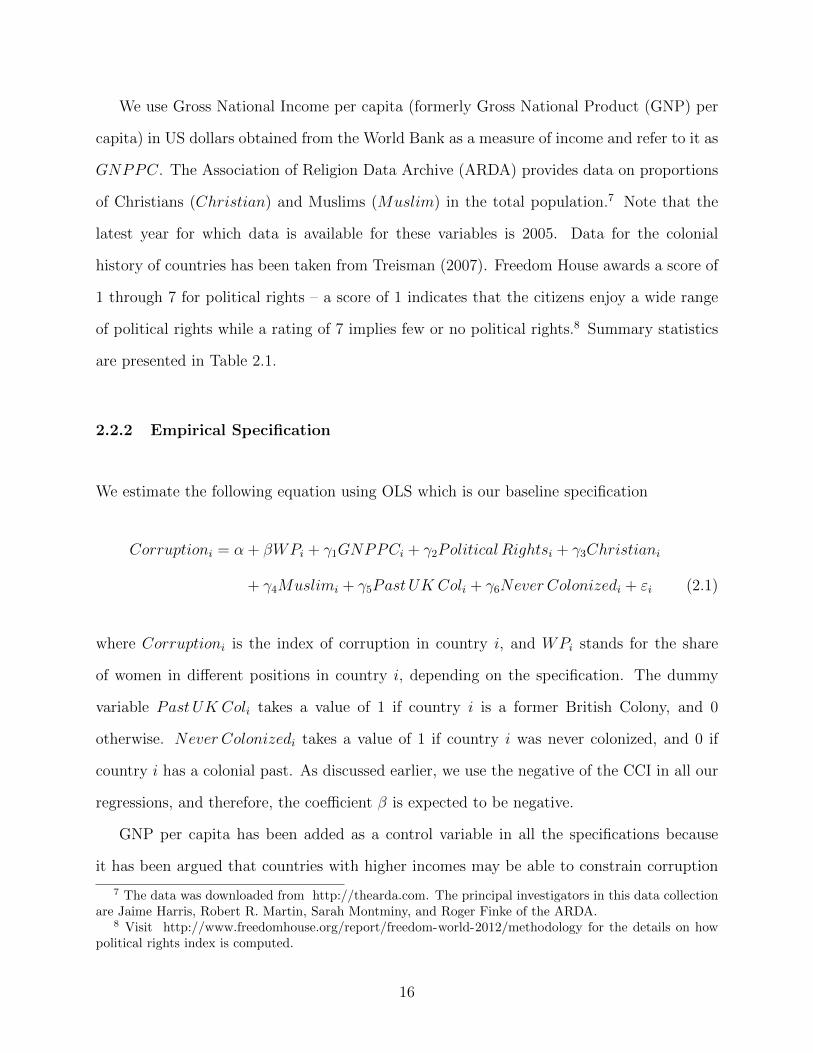
We use Gross National Income per capita (formerly Gross National Product (GNP) per
capita) in US dollars obtained from the World Bank as a measure of income and refer to it as
GNPPC. The Association of Religion Data Archive (ARDA) provides data on proportions
of Christians (Christian) and Muslims (Muslim) in the total population.7 Note that the
latest year for which data is available for these variables is 2005. Data for the colonial
history of countries has been taken from Treisman (2007). Freedom House awards a score of
1 through 7 for political rights – a score of 1 indicates that the citizens enjoy a wide range
of political rights while a rating of 7 implies few or no political rights.8 Summary statistics
are presented in Table 2.1.
2.2.2 Empirical Specification
We estimate the following equation using OLS which is our baseline specification
Corruptioni = α + βWPi + γ1GNPPCi + γ2Political Rightsi + γ3Christiani
+ γ4Muslimi + γ5Past UK Coli + γ6Never Colonizedi + εi (2.1)
where Corruptioni is the index of corruption in country i, and WPi stands for the share
of women in different positions in country i, depending on the specification. The dummy
variable Past UK Coli takes a value of 1 if country i is a former British Colony, and 0
otherwise. Never Colonizedi takes a value of 1 if country i was never colonized, and 0 if
country i has a colonial past. As discussed earlier, we use the negative of the CCI in all our
regressions, and therefore, the coefficient β is expected to be negative.
GNP per capita has been added as a control variable in all the specifications because
it has been argued that countries with higher incomes may be able to constrain corruption
7 The data was downloaded from http://thearda.com. The principal investigators in this data collectionare Jaime Harris, Robert R. Martin, Sarah Montminy, and Roger Finke of the ARDA.
8 Visit http://www.freedomhouse.org/report/freedom-world-2012/methodology for the details on howpolitical rights index is computed.
16
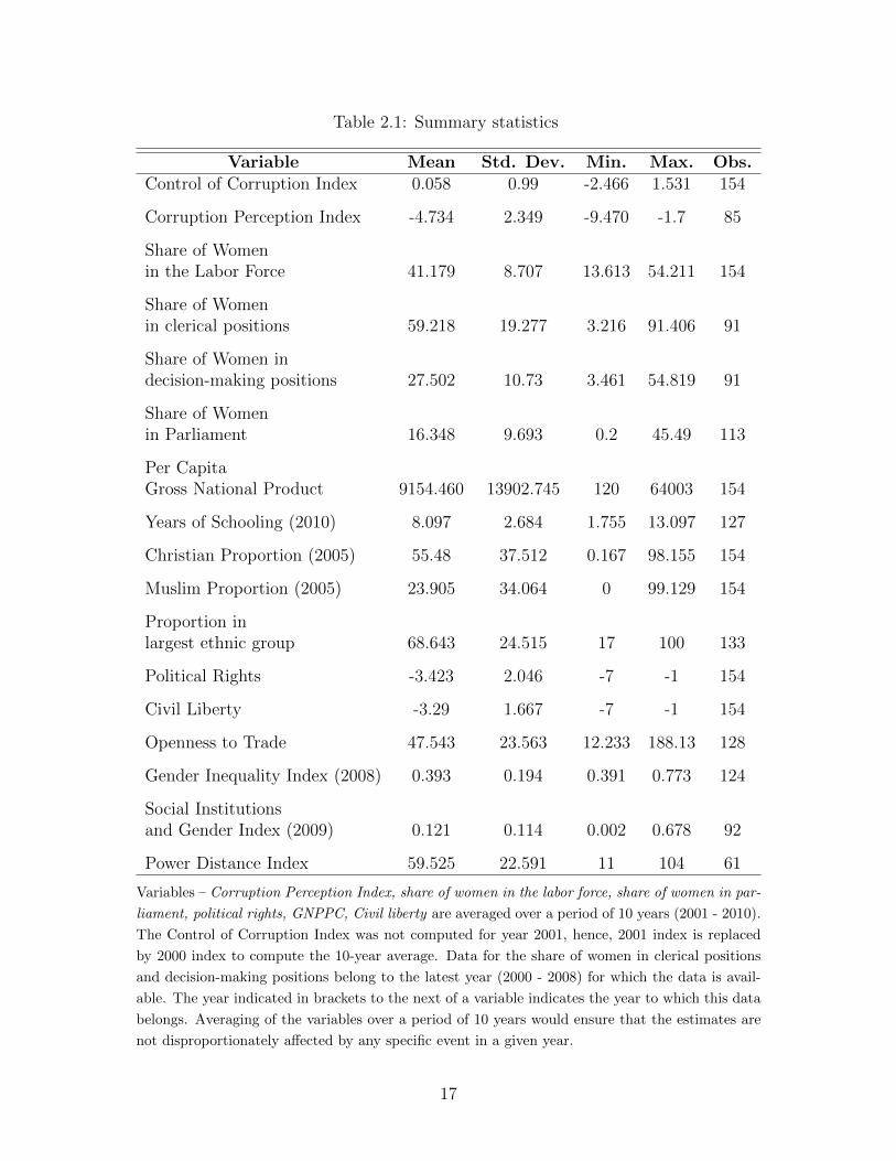
Table 2.1: Summary statistics
Variable Mean Std. Dev. Min. Max. Obs.Control of Corruption Index 0.058 0.99 -2.466 1.531 154
Corruption Perception Index -4.734 2.349 -9.470 -1.7 85
Share of Womenin the Labor Force 41.179 8.707 13.613 54.211 154
Share of Womenin clerical positions 59.218 19.277 3.216 91.406 91
Share of Women indecision-making positions 27.502 10.73 3.461 54.819 91
Share of Womenin Parliament 16.348 9.693 0.2 45.49 113
Per CapitaGross National Product 9154.460 13902.745 120 64003 154
Years of Schooling (2010) 8.097 2.684 1.755 13.097 127
Christian Proportion (2005) 55.48 37.512 0.167 98.155 154
Muslim Proportion (2005) 23.905 34.064 0 99.129 154
Proportion inlargest ethnic group 68.643 24.515 17 100 133
Political Rights -3.423 2.046 -7 -1 154
Civil Liberty -3.29 1.667 -7 -1 154
Openness to Trade 47.543 23.563 12.233 188.13 128
Gender Inequality Index (2008) 0.393 0.194 0.391 0.773 124
Social Institutionsand Gender Index (2009) 0.121 0.114 0.002 0.678 92
Power Distance Index 59.525 22.591 11 104 61
Variables – Corruption Perception Index, share of women in the labor force, share of women in par-
liament, political rights, GNPPC, Civil liberty are averaged over a period of 10 years (2001 - 2010).
The Control of Corruption Index was not computed for year 2001, hence, 2001 index is replaced
by 2000 index to compute the 10-year average. Data for the share of women in clerical positions
and decision-making positions belong to the latest year (2000 - 2008) for which the data is avail-
able. The year indicated in brackets to the next of a variable indicates the year to which this data
belongs. Averaging of the variables over a period of 10 years would ensure that the estimates are
not disproportionately affected by any specific event in a given year.
17
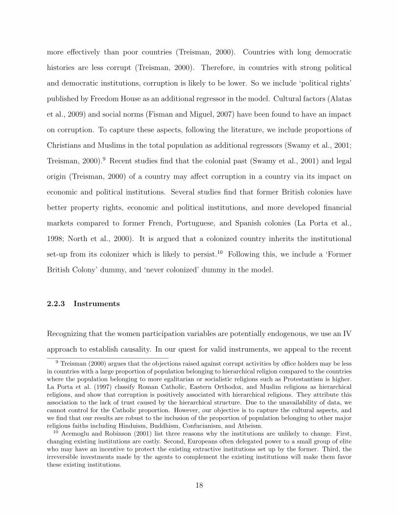
more effectively than poor countries (Treisman, 2000). Countries with long democratic
histories are less corrupt (Treisman, 2000). Therefore, in countries with strong political
and democratic institutions, corruption is likely to be lower. So we include ‘political rights’
published by Freedom House as an additional regressor in the model. Cultural factors (Alatas
et al., 2009) and social norms (Fisman and Miguel, 2007) have been found to have an impact
on corruption. To capture these aspects, following the literature, we include proportions of
Christians and Muslims in the total population as additional regressors (Swamy et al., 2001;
Treisman, 2000).9 Recent studies find that the colonial past (Swamy et al., 2001) and legal
origin (Treisman, 2000) of a country may affect corruption in a country via its impact on
economic and political institutions. Several studies find that former British colonies have
better property rights, economic and political institutions, and more developed financial
markets compared to former French, Portuguese, and Spanish colonies (La Porta et al.,
1998; North et al., 2000). It is argued that a colonized country inherits the institutional
set-up from its colonizer which is likely to persist.10 Following this, we include a ‘Former
British Colony’ dummy, and ‘never colonized’ dummy in the model.
2.2.3 Instruments
Recognizing that the women participation variables are potentially endogenous, we use an IV
approach to establish causality. In our quest for valid instruments, we appeal to the recent
9 Treisman (2000) argues that the objections raised against corrupt activities by office holders may be lessin countries with a large proportion of population belonging to hierarchical religion compared to the countrieswhere the population belonging to more egalitarian or socialistic religions such as Protestantism is higher.La Porta et al. (1997) classify Roman Catholic, Eastern Orthodox, and Muslim religions as hierarchicalreligions, and show that corruption is positively associated with hierarchical religions. They attribute thisassociation to the lack of trust caused by the hierarchical structure. Due to the unavailability of data, wecannot control for the Catholic proportion. However, our objective is to capture the cultural aspects, andwe find that our results are robust to the inclusion of the proportion of population belonging to other majorreligious faiths including Hinduism, Buddhism, Confucianism, and Atheism.
10 Acemoglu and Robinson (2001) list three reasons why the institutions are unlikely to change. First,changing existing institutions are costly. Second, Europeans often delegated power to a small group of elitewho may have an incentive to protect the existing extractive institutions set up by the former. Third, theirreversible investments made by the agents to complement the existing institutions will make them favorthese existing institutions.
18
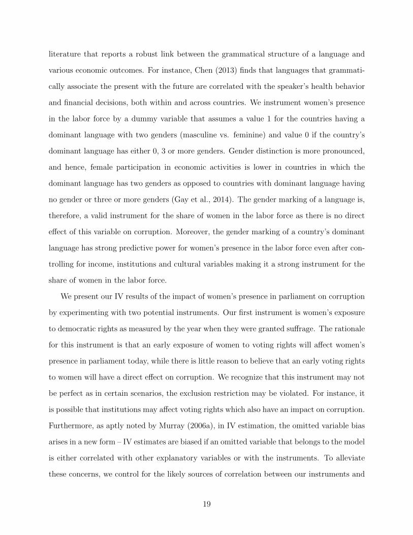
literature that reports a robust link between the grammatical structure of a language and
various economic outcomes. For instance, Chen (2013) finds that languages that grammati-
cally associate the present with the future are correlated with the speaker’s health behavior
and financial decisions, both within and across countries. We instrument women’s presence
in the labor force by a dummy variable that assumes a value 1 for the countries having a
dominant language with two genders (masculine vs. feminine) and value 0 if the country’s
dominant language has either 0, 3 or more genders. Gender distinction is more pronounced,
and hence, female participation in economic activities is lower in countries in which the
dominant language has two genders as opposed to countries with dominant language having
no gender or three or more genders (Gay et al., 2014). The gender marking of a language is,
therefore, a valid instrument for the share of women in the labor force as there is no direct
effect of this variable on corruption. Moreover, the gender marking of a country’s dominant
language has strong predictive power for women’s presence in the labor force even after con-
trolling for income, institutions and cultural variables making it a strong instrument for the
share of women in the labor force.
We present our IV results of the impact of women’s presence in parliament on corruption
by experimenting with two potential instruments. Our first instrument is women’s exposure
to democratic rights as measured by the year when they were granted suffrage. The rationale
for this instrument is that an early exposure of women to voting rights will affect women’s
presence in parliament today, while there is little reason to believe that an early voting rights
to women will have a direct effect on corruption. We recognize that this instrument may not
be perfect as in certain scenarios, the exclusion restriction may be violated. For instance, it
is possible that institutions may affect voting rights which also have an impact on corruption.
Furthermore, as aptly noted by Murray (2006a), in IV estimation, the omitted variable bias
arises in a new form – IV estimates are biased if an omitted variable that belongs to the model
is either correlated with other explanatory variables or with the instruments. To alleviate
these concerns, we control for the likely sources of correlation between our instruments and
19
the error term by including cultural, historical and contemporaneous controls, as well as
colonial and continent dummies.
Moreover, we employ a second instrument that allows us to check whether or not our
instruments are valid, conditional on either one of the instruments being valid. Our second
instrument, years since transition to agriculture, comes from a recent study (Hansen et al.,
2012) that finds that the societies that have long agricultural histories have more unequal
gender roles and lower participation of women in economic and political arenas including the
labor force and parliament. This is a valid instrument as we find that years since transition
to agriculture is indeed associated with lower participation of women in parliament, and at
the same time, there is no reason to expect that it can affect corruption directly. Mauritius
is the last country that adopted agriculture in our sample 375 years ago, while there are
countries that adopted agriculture as early as 10,500 years ago.
Though our instrument for the share of women in the labor force is strong, our instru-
ments for the share of women in parliament tend to be weak in some specifications which may
lead to invalid inferences. To counter this possibility, we use the Conditional Likelihood Ra-
tio (CLR) approach proposed by Moreira (2003) for hypothesis testing. Furthermore, while
under homoskedasticity, the CLR test is the most powerful test for hypothesis testing in the
presence of one endogenous variable and weak instruments, this result remains to be estab-
lished for other IV-type estimators (Murray, 2006a; Finlay and Magnusson, 2009). Hence, we
also report p−values for alternative approaches that provide robust inferences in the presence
of weak instruments such as LM-J (a combination of Kleibergen-Moreira Lagrange Multiplier
(LM) and the overidentification (J)-tests) (Kleibergen, 2002), and Anderson-Rubin (AR)
tests (Anderson and Rubin, 1949) against the null that the coefficient of the instrumented
variable, the share of women in parliament, is zero. In case of an over-identified equation, all
these three statistics test both the structural parameters and the overidentification restric-
tions simultaneously by combining the LM statistic and J statistic, and provide inferences
that are robust to the presence of weak instruments.
20
2.3 Cross-country results
2.3.1 OLS evidence
A. Women in the labor force and corruption
First, we investigate the relationship between the share of women in the labor force and
corruption. The first column of Table 2.2 presents the result of the baseline specification
with the variable of interest being the share of women in the labor force. The coefficient on
the share of women in the labor force is negative and significant at the 5% level. However,
when we include continent dummies in column 2, coefficient of the share of women in the
labor force is no longer significant though it has expected sign.11
B. Women in potential bribe-taking positions and corruption
As shown in Table 2.2 (column 3), we do not find any significant association between the
share of women in clerical positions and corruption which suggests that the bribe-taking role
of women is not significant in determining the relationship between female participation in
the labor force and corruption.
C. Women in decision-making positions and corruption
Next, we investigate whether decision-making ability allows women to impact corruption.
This position captures both the bribe-giving and demanding role: While women in the
positions of senior managers and officials are likely to be bribe-givers; women as legislators
and senior government officials are likely to be bribe-takers. Hence, if women are less corrupt,
we should observe a strong and negative association between this variable and corruption.
We, however, find no association between the share of women in decision-making positions
and corruption (column 4 of Table 2.2). We also do not find corruption to be significantly
associated with either the share of women in clerical positions or the share of women in
decision-making positions when continent dummies are added to the model (results omitted).
11 Continent dummies are: Africa (the omitted category), Asia, Europe, North America, Oceania, SouthAmerica, and Sub-Saharan Africa.
21
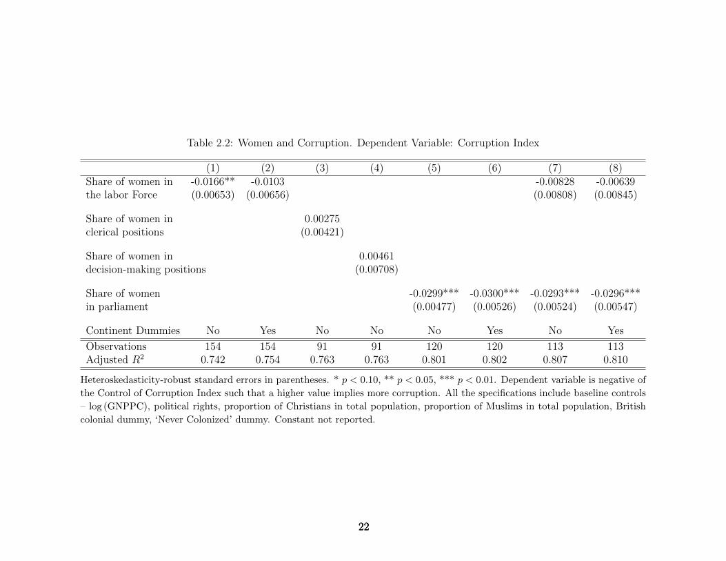
Table 2.2: Women and Corruption. Dependent Variable: Corruption Index
(1) (2) (3) (4) (5) (6) (7) (8)Share of women in -0.0166** -0.0103 -0.00828 -0.00639the labor Force (0.00653) (0.00656) (0.00808) (0.00845)
Share of women in 0.00275clerical positions (0.00421)
Share of women in 0.00461decision-making positions (0.00708)
Share of women -0.0299*** -0.0300*** -0.0293*** -0.0296***in parliament (0.00477) (0.00526) (0.00524) (0.00547)
Continent Dummies No Yes No No No Yes No Yes
Observations 154 154 91 91 120 120 113 113Adjusted R2 0.742 0.754 0.763 0.763 0.801 0.802 0.807 0.810
Heteroskedasticity-robust standard errors in parentheses. * p < 0.10, ** p < 0.05, *** p < 0.01. Dependent variable is negative of
the Control of Corruption Index such that a higher value implies more corruption. All the specifications include baseline controls
– log (GNPPC), political rights, proportion of Christians in total population, proportion of Muslims in total population, British
colonial dummy, ‘Never Colonized’ dummy. Constant not reported.
222222
D. Women in parliament and corruption
Finally, we investigate if women can have an impact on corruption by being in the
role of policy makers. Consistent with the findings of the previous studies, we present
evidence of a significant and negative association between the share of women in parliament
and corruption. The coefficient of the share of women in parliament is found to be highly
significant with the expected sign (column 5). Moreover, this relationship is robust to the
inclusion of the continent dummies in column 6. Finally, column 7 controls for both the
variables – women’s share in the labor force and their presence in parliament. As we can see,
the coefficient of the share of women in the labor force is very small and insignificant. On
the other hand, the coefficient of women’s participation in parliament remains significant.
Results remain unchanged when continent dummies are added in column 8.
Notice that the regressions with women in decision-making positions and clerical positions
as variables of interest have a considerably smaller sample size of 91 countries because of the
data unavailability. It may be possible that the loss of observations in these regressions is
non-random and the lack of significance is driven by sample selection. Table 2.3 restricts the
analysis to only those countries for which data is available for all the women’s participation
variables and finds similar results except that women’s share in the labor force now has
a significant sign even when the continent dummies are controlled for. However, it loses
significance in column 7 when both the share of women in parliament and the share of
women in the labor force is included in the same specification. To be consistent with Table
2.2, continent dummies are added in column 8: the coefficient of the share of women in the
labor force remains insignificant.
E. Inclusion of additional variables
Next, we control for a number of variables in order to minimize the possibility of omitted
variable bias as well as to address the concerns of some of the previous studies that hypoth-
esize that the relationship between female participation variables and corruption is spurious
and is driven by the omission of relevant variables. These results are presented in Table 2.4.
23
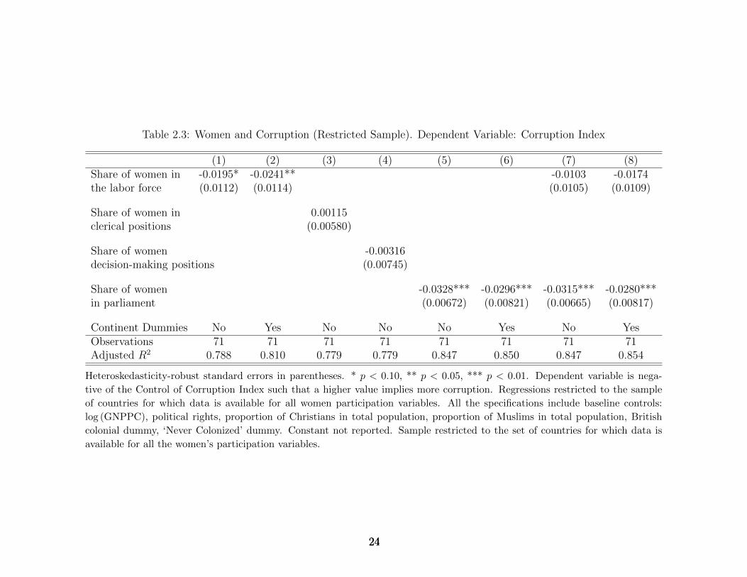
Table 2.3: Women and Corruption (Restricted Sample). Dependent Variable: Corruption Index
(1) (2) (3) (4) (5) (6) (7) (8)Share of women in -0.0195* -0.0241** -0.0103 -0.0174the labor force (0.0112) (0.0114) (0.0105) (0.0109)
Share of women in 0.00115clerical positions (0.00580)
Share of women -0.00316decision-making positions (0.00745)
Share of women -0.0328*** -0.0296*** -0.0315*** -0.0280***in parliament (0.00672) (0.00821) (0.00665) (0.00817)
Continent Dummies No Yes No No No Yes No YesObservations 71 71 71 71 71 71 71 71Adjusted R2 0.788 0.810 0.779 0.779 0.847 0.850 0.847 0.854
Heteroskedasticity-robust standard errors in parentheses. * p < 0.10, ** p < 0.05, *** p < 0.01. Dependent variable is nega-
tive of the Control of Corruption Index such that a higher value implies more corruption. Regressions restricted to the sample
of countries for which data is available for all women participation variables. All the specifications include baseline controls:
log (GNPPC), political rights, proportion of Christians in total population, proportion of Muslims in total population, British
colonial dummy, ‘Never Colonized’ dummy. Constant not reported. Sample restricted to the set of countries for which data is
available for all the women’s participation variables.
242424
Liberal democracy: Sung (2003) argues that, in liberal democracies, women’s partic-
ipation is higher and corruption is lower, and it is the omission of the liberal democratic
institutions variable that may be responsible for the relationship between female participa-
tion and corruption.12 We address this concern by replacing the political rights variable with
the civil liberties index published by Freedom House. It takes a value from 1 (high civil
liberties) through 7 (low civil liberties) and is a broader measure of liberal democracy than
political rights.13 The index takes into account, among other things, the personal and social
freedom of women including their choice of marriage partners and say in the family size. The
coefficient of both the female participation variables remains significant when this variable
is controlled for in columns 1 and 7.
Power structure and corruption: Different cultures have varied levels of tolerance
for an unequal distribution of power. Hofstede’s Power Distance Index (PDI) measures
this tolerance providing a score in the range of 0 to 120, with the higher value indicating
tolerance for a hierarchical order while a lower value implies that people strive to equalize
the distribution of power.14 We control for the PDI as an alternative measure of cultural
differences among countries, and find that while women’s share in parliament remains highly
significant (column 8), women’s share in the labor force is no longer significant (column 2).
Gender-biased institutions and corruption: It has been hypothesized that social
institutions that discourage female participation in political and economic spheres are also
more corrupt (Branisa et al., 2013). Hence, to address the concerns that our results may
have been driven by the omission of gender-biased institutions, we control for the Social
Institutions and Gender Index (SIGI). SIGI is a measure of gender inequality attributed to
institutions and was first launched in 2009 by the Organisation for Economic Co-operation
and Development (OECD). It is composite measure of five subindices – family code, civil lib-
12 In a recent study, Esarey and Chirillo (2013) argue that women are more likely to conform to thepolitical and institutional norms, and find evidence that the relationship between gender and corruptiondepends on the institutional context.
13 For details on the differences between the two indices and how they are computed, visit Freedom Housewebsite: http://www.freedomhouse.org/report/freedom-world-2012/methodology.
14 Visit http://geert-hofstede.com/dimensions.html for details.
25

erties, physical integrity, son-preference and ownership index. The family code is a measure
of women’s decision making power in the household on following issues – parental author-
ity, inheritance, early marriage, and polygamy. Freedom of social participation of women
including ‘freedom of movement’ and ‘freedom of dress’ is captured by the civil liberties sub-
index. Note that this civil liberties index is different from the civil liberty index (discussed
later) as published by the Freedom House. The ‘violence against women’ and ‘female genital
mutilation’ are captured by the physical integrity measure. The sub-index son preference,
as the name suggests, shows the preference for male child under scarce resources. It takes
the value of the variable ‘missing women’ that reflects the gender bias in mortality. Finally,
the sub-index ownership rights measures women’s access to property and includes ‘women’s
access to land,’ ‘women’s access to bank loans,’ and ‘women’s access to property other than
land’. Further details regarding the construction of SIGI can be found in Branisa et al.
(2009) and Branisa et al. (2013). Branisa et al. (2013) state that “...we believe that the
SIGI and its sub-components well capture gender inequality in social institutions which have
previously not been adequately captured...”.
The SIGI, thus, captures “discriminatory social institutions, such as early marriage, dis-
criminatory inheritance practices, violence against women, son preference, restricted access
to public space and restricted access to land and credit.” The index takes a value from 0 to
1, with 1 representing high inequality. The inclusion of SIGI causes the share of women in
the labor force to be close to zero and insignificant in column 3. The coefficient of the share
of women in parliament, however, remains sizable and significant in column 9.
Schooling, ethnic division, and corruption: Columns 4 and 10 control for two
additional covariates – ‘proportion in largest ethnic group’ and ‘average years of schooling’.
The proportion of the population belonging to the largest ethnic groups (Ethnic) is taken
from Sullivan (1991). While the World Bank publishes data on schooling, the coverage of
countries in Barro-Lee (Barro and Lee, 2013) data set is broader making it our preferred
source for schooling data. We use average years of schooling (Education) data for the year
26
2010 as the Barro-Lee educational attainment data is available only for 5-year intervals. Our
results are, however, robust when we use the proportion of the population with the secondary
education or tertiary education, instead of the years of the average years of schooling attained
by the population. Corruption may be higher in countries that are more ethnically divided,
and lower in countries with higher human capital where people are aware of their legal and
constitutional rights.
The negative relationship between women’s participation variables and corruption is ro-
bust to the inclusion of these variables. Their coefficient of women’s share in the labor force
as well as parliament remains significant in columns 4 and 10 respectively. However, once
we add continent dummies along with these variables, the share of women in the labor force
loses significance (column 5), while the share of women in parliament remains statistically
significant in column 11.
Openness to trade: It has been found that countries that are more open and have
lower barriers to international trade are less corrupt (Ades and Di Tella, 1999; Treisman,
2000). Hence, we include the share of imports of goods and services in GDP as a measure
of openness to trade. We take this data from the World Bank. We find that the share of
women in parliament (column 12) is significant; while women’s share in the labor force is
not significant at conventional levels (column 6).
Notice that we have a smaller sample when the variable of interest is the share of women
in parliament compared to the specifications in which the variable of interest is the share
of women in the labor force. In order to rule out the concern that sample selection is
responsible for the differences in the significance of the two variables, we re-run the regression
specifications in columns 1-6 restricting the sample to the countries that are included in
columns 7-12. The results are presented in Table 2.5 and are similar to those presented in
columns 1-6 in Table 2.4 – the share of women in the labor force is significantly associated
with corruption in columns 1 and 4 but is insignificant in columns 2, 3, 5 and 6.
27
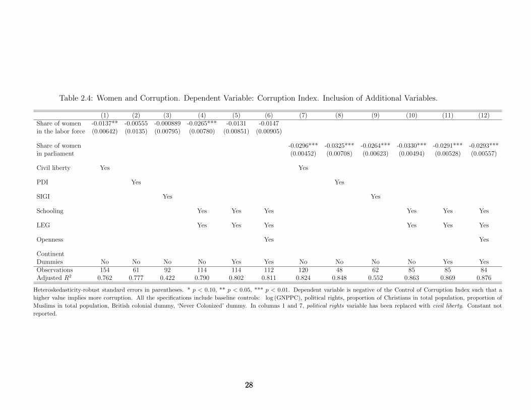
Table 2.4: Women and Corruption. Dependent Variable: Corruption Index. Inclusion of Additional Variables.
(1) (2) (3) (4) (5) (6) (7) (8) (9) (10) (11) (12)Share of women -0.0137** -0.00555 -0.000889 -0.0265*** -0.0131 -0.0147in the labor force (0.00642) (0.0135) (0.00795) (0.00780) (0.00851) (0.00905)
Share of women -0.0296*** -0.0325*** -0.0264*** -0.0330*** -0.0291*** -0.0293***in parliament (0.00452) (0.00708) (0.00623) (0.00494) (0.00528) (0.00557)
Civil liberty Yes Yes
PDI Yes Yes
SIGI Yes Yes
Schooling Yes Yes Yes Yes Yes Yes
LEG Yes Yes Yes Yes Yes Yes
Openness Yes Yes
ContinentDummies No No No No Yes Yes No No No No Yes YesObservations 154 61 92 114 114 112 120 48 62 85 85 84Adjusted R2 0.762 0.777 0.422 0.790 0.802 0.811 0.824 0.848 0.552 0.863 0.869 0.876
Heteroskedasticity-robust standard errors in parentheses. * p < 0.10, ** p < 0.05, *** p < 0.01. Dependent variable is negative of the Control of Corruption Index such that a
higher value implies more corruption. All the specifications include baseline controls: log (GNPPC), political rights, proportion of Christians in total population, proportion of
Muslims in total population, British colonial dummy, ‘Never Colonized’ dummy. In columns 1 and 7, political rights variable has been replaced with civil liberty. Constant not
reported.
282828
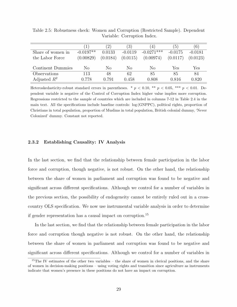
Table 2.5: Robustness check: Women and Corruption (Restricted Sample). DependentVariable: Corruption Index.
(1) (2) (3) (4) (5) (6)Share of women in -0.0197** 0.0133 -0.0119 -0.0271*** -0.0175 -0.0181the Labor Force (0.00829) (0.0184) (0.0115) (0.00974) (0.0117) (0.0123)
Continent Dummies No No No No Yes YesObservations 113 48 62 85 85 84Adjusted R2 0.778 0.791 0.458 0.808 0.816 0.820
Heteroskedasticity-robust standard errors in parentheses. * p < 0.10, ** p < 0.05, *** p < 0.01. De-
pendent variable is negative of the Control of Corruption Index higher value implies more corruption.
Regressions restricted to the sample of countries which are included in columns 7-12 in Table 2.4 in the
main text. All the specifications include baseline controls: log (GNPPC), political rights, proportion of
Christians in total population, proportion of Muslims in total population, British colonial dummy, ‘Never
Colonized’ dummy. Constant not reported.
2.3.2 Establishing Causality: IV Analysis
In the last section, we find that the relationship between female participation in the labor
force and corruption, though negative, is not robust. On the other hand, the relationship
between the share of women in parliament and corruption was found to be negative and
significant across different specifications. Although we control for a number of variables in
the previous section, the possibility of endogeneity cannot be entirely ruled out in a cross-
country OLS specification. We now use instrumental variable analysis in order to determine
if gender representation has a causal impact on corruption.15
In the last section, we find that the relationship between female participation in the labor
force and corruption though negative is not robust. On the other hand, the relationship
between the share of women in parliament and corruption was found to be negative and
significant across different specifications. Although we control for a number of variables in
15The IV estimates of the other two variables – the share of women in clerical positions, and the shareof women in decision-making positions – using voting rights and transition since agriculture as instrumentsindicate that women’s presence in these positions do not have an impact on corruption.
29
the previous section, the possibility of endogeneity cannot be entirely ruled out in a cross-
country OLS specification. We now use instrumental variable analysis in order to determine
if gender representation has a causal impact on corruption.16
A. Women in the labor force and corruption
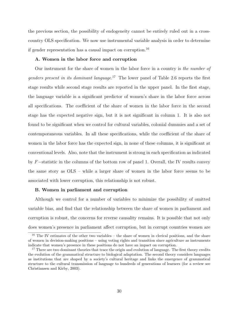
Our instrument for the share of women in the labor force in a country is the number of
genders present in its dominant language.17 The lower panel of Table 2.6 reports the first
stage results while second stage results are reported in the upper panel. In the first stage,
the language variable is a significant predictor of women’s share in the labor force across
all specifications. The coefficient of the share of women in the labor force in the second
stage has the expected negative sign, but it is not significant in column 1. It is also not
found to be significant when we control for cultural variables, colonial dummies and a set of
contemporaneous variables. In all these specifications, while the coefficient of the share of
women in the labor force has the expected sign, in none of these columns, it is significant at
conventional levels. Also, note that the instrument is strong in each specification as indicated
by F−statistic in the columns of the bottom row of panel 1. Overall, the IV results convey
the same story as OLS – while a larger share of women in the labor force seems to be
associated with lower corruption, this relationship is not robust.
B. Women in parliament and corruption
Although we control for a number of variables to minimize the possibility of omitted
variable bias, and find that the relationship between the share of women in parliament and
corruption is robust, the concerns for reverse causality remains. It is possible that not only
does women’s presence in parliament affect corruption, but in corrupt countries women are
16 The IV estimates of the other two variables – the share of women in clerical positions, and the shareof women in decision-making positions – using voting rights and transition since agriculture as instrumentsindicate that women’s presence in these positions do not have an impact on corruption.
17 There are two dominant theories that trace the origin and evolution of language. The first theory creditsthe evolution of the grammatical structure to biological adaptation. The second theory considers languagesas institutions that are shaped by a society’s cultural heritage and links the emergence of grammaticalstructure to the cultural transmission of language to hundreds of generations of learners (for a review seeChristiansen and Kirby, 2003).
30
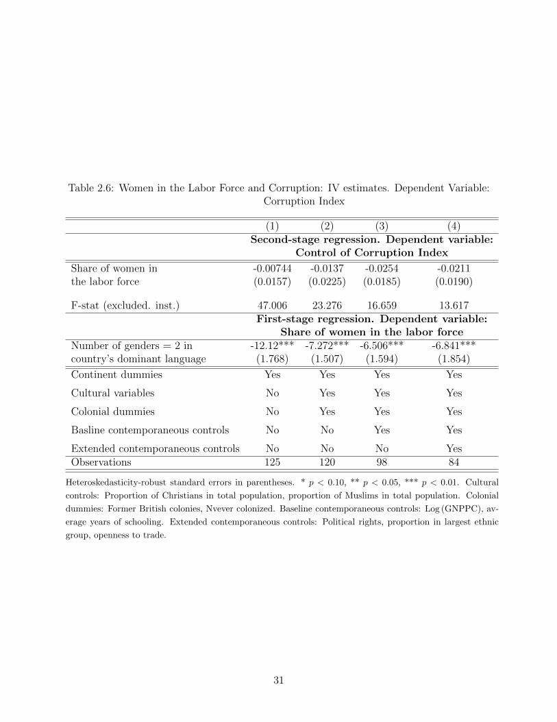
Table 2.6: Women in the Labor Force and Corruption: IV estimates. Dependent Variable:Corruption Index
(1) (2) (3) (4)Second-stage regression. Dependent variable:
Control of Corruption Index
Share of women in -0.00744 -0.0137 -0.0254 -0.0211the labor force (0.0157) (0.0225) (0.0185) (0.0190)
F-stat (excluded. inst.) 47.006 23.276 16.659 13.617First-stage regression. Dependent variable:
Share of women in the labor forceNumber of genders = 2 in -12.12*** -7.272*** -6.506*** -6.841***country’s dominant language (1.768) (1.507) (1.594) (1.854)
Continent dummies Yes Yes Yes Yes
Cultural variables No Yes Yes Yes
Colonial dummies No Yes Yes Yes
Basline contemporaneous controls No No Yes Yes
Extended contemporaneous controls No No No YesObservations 125 120 98 84
Heteroskedasticity-robust standard errors in parentheses. * p < 0.10, ** p < 0.05, *** p < 0.01. Cultural
controls: Proportion of Christians in total population, proportion of Muslims in total population. Colonial
dummies: Former British colonies, Nvever colonized. Baseline contemporaneous controls: Log (GNPPC), av-
erage years of schooling. Extended contemporaneous controls: Political rights, proportion in largest ethnic
group, openness to trade.
31
also discouraged from participating in politics.18 If this is true, our OLS estimates will be
biased. To address this issue, we use instruments for women’s presence in parliament.
First, we present IV estimates by instrumenting women’s participation in parliament
with “the year women were granted voting rights”. An initiative to include women in the
political process should be positively correlated with their presence in politics and in national
parliaments.
Figure 2.1: Voting Rights and Presence of Women in Parliament
Figure 2.1 shows a scatter plot of the association between the year women were granted
suffrage and their presence in parliament. New Zealand is the first country to allow women
to vote in 1893, and the State of Kuwait was the last country (in our sample) to grant
voting rights to women in 2005.19 However, there still might be some concerns about omitted
18 Sundstrom and Wangnerud (2014) find that greater corruption is associated with lower political repre-sentation of women.
19 The State of Kuwait granted voting rights to women on the condition that they observe Islamic laws.See the link for additional details, http://www.cnn.com/2005/WORLD/meast/05/16/kuwait.women/. This
32
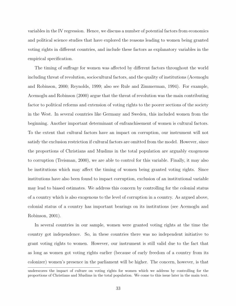
variables in the IV regression. Hence, we discuss a number of potential factors from economics
and political science studies that have explored the reasons leading to women being granted
voting rights in different countries, and include these factors as explanatory variables in the
empirical specification.
The timing of suffrage for women was affected by different factors throughout the world
including threat of revolution, sociocultural factors, and the quality of institutions (Acemoglu
and Robinson, 2000; Reynolds, 1999; also see Rule and Zimmerman, 1994). For example,
Acemoglu and Robinson (2000) argue that the threat of revolution was the main contributing
factor to political reforms and extension of voting rights to the poorer sections of the society
in the West. In several countries like Germany and Sweden, this included women from the
beginning. Another important determinant of enfranchisement of women is cultural factors.
To the extent that cultural factors have an impact on corruption, our instrument will not
satisfy the exclusion restriction if cultural factors are omitted from the model. However, since
the proportions of Christians and Muslims in the total population are arguably exogenous
to corruption (Treisman, 2000), we are able to control for this variable. Finally, it may also
be institutions which may affect the timing of women being granted voting rights. Since
institutions have also been found to impact corruption, exclusion of an institutional variable
may lead to biased estimates. We address this concern by controlling for the colonial status
of a country which is also exogenous to the level of corruption in a country. As argued above,
colonial status of a country has important bearings on its institutions (see Acemoglu and
Robinson, 2001).
In several countries in our sample, women were granted voting rights at the time the
country got independence. So, in these countries there was no independent initiative to
grant voting rights to women. However, our instrument is still valid due to the fact that
as long as women got voting rights earlier (because of early freedom of a country from its
colonizer) women’s presence in the parliament will be higher. The concern, however, is that
underscores the impact of culture on voting rights for women which we address by controlling for theproportions of Christians and Muslims in the total population. We come to this issue later in the main text.
33
in these countries women’s presence in parliament may also be capturing the impact of a
change in democratic status of these countries since the independence year and women’s
participation in parliament are correlated. Since the year of independence of a country is
exogenous, we control for the year of independence to rule out the possibility of any bias
arising from this. Data for the year of independence has been taken from Acemoglu et al.
who set any year before 1800 as 1800 (see Acemoglu et al., 2008 for details).
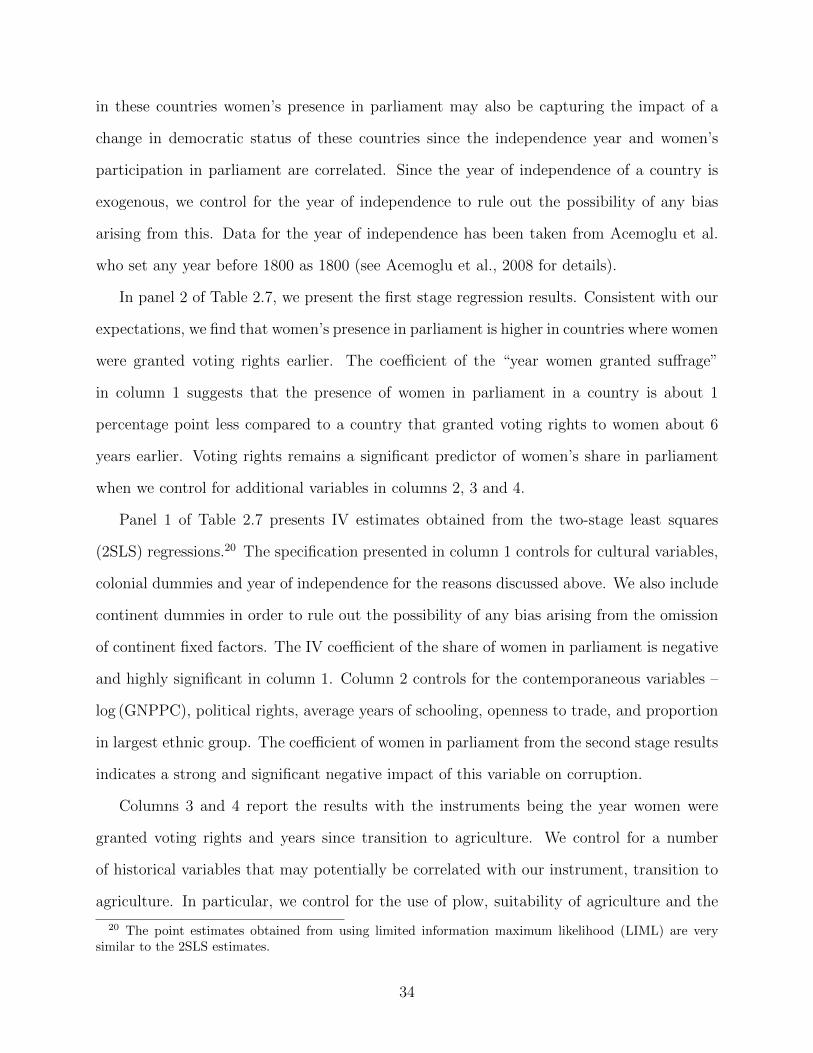
In panel 2 of Table 2.7, we present the first stage regression results. Consistent with our
expectations, we find that women’s presence in parliament is higher in countries where women
were granted voting rights earlier. The coefficient of the “year women granted suffrage”
in column 1 suggests that the presence of women in parliament in a country is about 1
percentage point less compared to a country that granted voting rights to women about 6
years earlier. Voting rights remains a significant predictor of women’s share in parliament
when we control for additional variables in columns 2, 3 and 4.
Panel 1 of Table 2.7 presents IV estimates obtained from the two-stage least squares
(2SLS) regressions.20 The specification presented in column 1 controls for cultural variables,
colonial dummies and year of independence for the reasons discussed above. We also include
continent dummies in order to rule out the possibility of any bias arising from the omission
of continent fixed factors. The IV coefficient of the share of women in parliament is negative
and highly significant in column 1. Column 2 controls for the contemporaneous variables –
log (GNPPC), political rights, average years of schooling, openness to trade, and proportion
in largest ethnic group. The coefficient of women in parliament from the second stage results
indicates a strong and significant negative impact of this variable on corruption.
Columns 3 and 4 report the results with the instruments being the year women were
granted voting rights and years since transition to agriculture. We control for a number
of historical variables that may potentially be correlated with our instrument, transition to
agriculture. In particular, we control for the use of plow, suitability of agriculture and the
20 The point estimates obtained from using limited information maximum likelihood (LIML) are verysimilar to the 2SLS estimates.
34
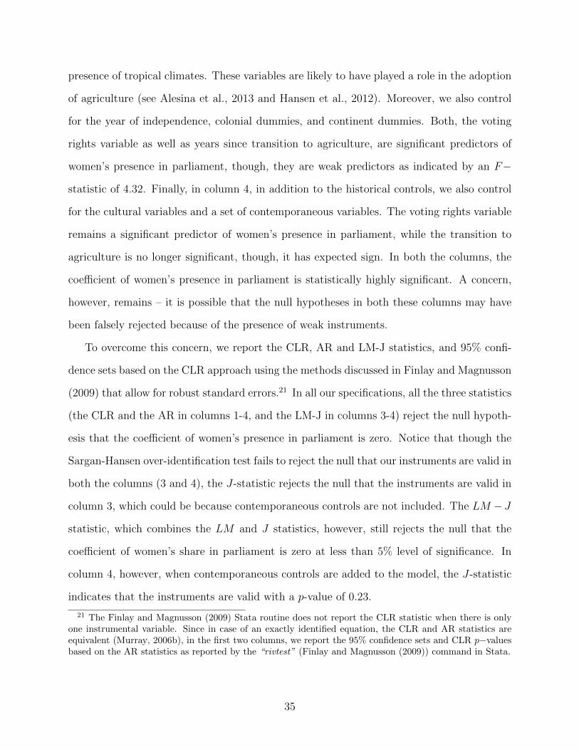
presence of tropical climates. These variables are likely to have played a role in the adoption
of agriculture (see Alesina et al., 2013 and Hansen et al., 2012). Moreover, we also control
for the year of independence, colonial dummies, and continent dummies. Both, the voting
rights variable as well as years since transition to agriculture, are significant predictors of
women’s presence in parliament, though, they are weak predictors as indicated by an F−
statistic of 4.32. Finally, in column 4, in addition to the historical controls, we also control
for the cultural variables and a set of contemporaneous variables. The voting rights variable
remains a significant predictor of women’s presence in parliament, while the transition to
agriculture is no longer significant, though, it has expected sign. In both the columns, the
coefficient of women’s presence in parliament is statistically highly significant. A concern,
however, remains – it is possible that the null hypotheses in both these columns may have
been falsely rejected because of the presence of weak instruments.
To overcome this concern, we report the CLR, AR and LM-J statistics, and 95% confi-
dence sets based on the CLR approach using the methods discussed in Finlay and Magnusson
(2009) that allow for robust standard errors.21 In all our specifications, all the three statistics
(the CLR and the AR in columns 1-4, and the LM-J in columns 3-4) reject the null hypoth-
esis that the coefficient of women’s presence in parliament is zero. Notice that though the
Sargan-Hansen over-identification test fails to reject the null that our instruments are valid in
both the columns (3 and 4), the J-statistic rejects the null that the instruments are valid in
column 3, which could be because contemporaneous controls are not included. The LM − J
statistic, which combines the LM and J statistics, however, still rejects the null that the
coefficient of women’s share in parliament is zero at less than 5% level of significance. In
column 4, however, when contemporaneous controls are added to the model, the J-statistic
indicates that the instruments are valid with a p-value of 0.23.
21 The Finlay and Magnusson (2009) Stata routine does not report the CLR statistic when there is onlyone instrumental variable. Since in case of an exactly identified equation, the CLR and AR statistics areequivalent (Murray, 2006b), in the first two columns, we report the 95% confidence sets and CLR p−valuesbased on the AR statistics as reported by the “rivtest” (Finlay and Magnusson (2009)) command in Stata.
35
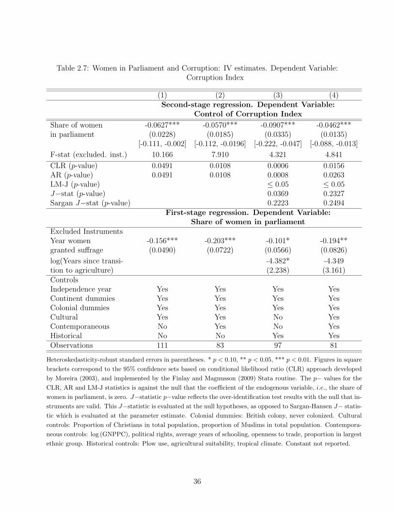
Table 2.7: Women in Parliament and Corruption: IV estimates. Dependent Variable:Corruption Index
(1) (2) (3) (4)Second-stage regression. Dependent Variable:
Control of Corruption Index
Share of women -0.0627*** -0.0570*** -0.0907*** -0.0462***in parliament (0.0228) (0.0185) (0.0335) (0.0135)
[-0.111, -0.002] [-0.112, -0.0196] [-0.222, -0.047] [-0.088, -0.013]
F-stat (excluded. inst.) 10.166 7.910 4.321 4.841
CLR (p-value) 0.0491 0.0108 0.0006 0.0156AR (p-value) 0.0491 0.0108 0.0008 0.0263LM-J (p-value) ≤ 0.05 ≤ 0.05J−stat (p-value) 0.0369 0.2327Sargan J−stat (p-value) 0.2223 0.2494
First-stage regression. Dependent Variable:Share of women in parliament
Excluded InstrumentsYear women -0.156*** -0.203*** -0.101* -0.194**granted suffrage (0.0490) (0.0722) (0.0566) (0.0826)
log(Years since transi- -4.382* -4.349tion to agriculture) (2.238) (3.161)ControlsIndependence year Yes Yes Yes YesContinent dummies Yes Yes Yes YesColonial dummies Yes Yes Yes YesCultural Yes Yes No YesContemporaneous No Yes No YesHistorical No No Yes YesObservations 111 83 97 81
Heteroskedasticity-robust standard errors in parentheses. * p < 0.10, ** p < 0.05, *** p < 0.01. Figures in square
brackets correspond to the 95% confidence sets based on conditional likelihood ratio (CLR) approach developed
by Moreira (2003), and implemented by the Finlay and Magnusson (2009) Stata routine. The p− values for the
CLR, AR and LM-J statistics is against the null that the coefficient of the endogenous variable, i.e., the share of
women in parliament, is zero. J−statistic p−value reflects the over-identification test results with the null that in-
struments are valid. This J−statistic is evaluated at the null hypotheses, as opposed to Sargan-Hansen J− statis-
tic which is evaluated at the parameter estimate. Colonial dummies: British colony, never colonized. Cultural
controls: Proportion of Christians in total population, proportion of Muslims in total population. Contempora-
neous controls: log (GNPPC), political rights, average years of schooling, openness to trade, proportion in largest
ethnic group. Historical controls: Plow use, agricultural suitability, tropical climate. Constant not reported.
36
The IV findings can be summarized as follows. First, the coefficient of women’s presence
in parliament is always highly significant in all the specifications, irrespective of the instru-
ments used. Second, across all the specifications, the CLR statistic rejects the null that the
coefficient of the share of women in parliament is zero. Third, the IV coefficients of women’s
share in parliament are always greater than the OLS coefficient reported in the previous
section indicating that the OLS estimates of the effect of women’s presence in parliament on
corruption may be the lower bound.
2.3.3 Robustness Check
We limit our robustness checks to the two main variables of interest that have been found
to be significantly associated with corruption in the previous section: the share of women in
the labor force and the share of women in parliament.
Sensitivity to alternative measure of corruption
We check the sensitivity of our results with the use of an alternative measure of cor-
ruption, the Corruption Perception Index (CPI), published by Transparency International
which defines it as “the misuse of public power for private benefit.” It takes values in the
range of 0 to 10, with a higher value indicating a lower level of corruption. We use negative
of the CPI so that a higher number indicates higher corruption. CPI is created using data
from different surveys conducted by a number of independent sources making it reliable and
one of the most widely used indices in empirical corruption literature. In order to ensure
reliability and robustness of the index, CPI ranks only those countries which are covered
by a minimum of three different sources. Unlike CCI, in compiling the CPI all the sources
are assigned equal weight. The surveys used in the compilation of the CPI are primarily
of two types: opinion surveys of business men, and assessment scores assigned by a group
of country, risk, or expert analysts.22 While survey questions differ among several data
22 The CPI method was developed by Johann Lambsdorff of the University of Passau. For the detailedmethodology of computation of 2009 corruption perception index, visit http://archive.transparency.org/
37
sources, the objective of all the sources is to measure the prevalence of corruption as defined
by Transparency International.23
The corruption perception indices (both the CCI and CPI) are often criticized on the
grounds that they might be infected with the problem of circularity: While responding to
survey questions, individuals’ might “go with the herd” and their responses may be driven
by the values of the past index. An advantage of using the CPI is that this hypothesis was
tested and rejected in 2006 implying that the CPI reflects the perceptions which represent
actual experience and not hearsay and, therefore, “the perceptions gathered are a helpful
contribution to the understanding of real levels of corruption” (Lambsdorff, 2008; also see
Lambsdorff (2007) for a discussion). The two indices, the CCI and CPI, have a correlation
coefficient greater than 0.98 in the sample of countries used in this chapter. The high
correlation between the two indices is not surprising following the fact that there are various
common data sources in the computation of the two indices.24
Table 2.8 reports the results of the OLS, median, and robust regressions using CPI. These
results are in agreement with our findings using the CCI – while the coefficient of women’s
presence in parliament is highly significant and negative regardless of the regression type
and inclusion of the continent dummies (columns 3, 4, 6, and 8), the coefficient of the share
of women in the labor force is not (columns 1, 2, 5, and 7). Moreover, corruption is not
found to be significantly associated with the share of women in either clerical positions or
decision-making positions and hence these results are not reported.
policy research/surveys indices/cpi/2009/methodology.23 Some of the questions reflected in the 2009 CPI scores are following – “To what extent are there legal
or political penalties for officeholders who abuse their positions?” “In your country, how commonly do thefollowing firms (domestic and foreign firms) pay bribes to public servants or public officials?” “To whatextent can the government successfully contain corruption?” “To what extent you agree that “Bribing andcorruption” exist or not in the context of the country in which you work, and have resided for the pastyear, based on your previous international experience.” Most of these questions ask respondents to assign anumber in a given range, where a number is an indication of the extent to which the respondent agrees tothe statement (question).
24 For instance, some of the common data sources are: African Development Bank (Country Policyand Institutional Assessments), Asian Development Bank (Country Policy and Institutional Assessments),Bertelsmann Foundation, Economist Intelligence Unit, Freedom House, Global Insight, Political & EconomicRisk Consultancy, World Economic Forum Global Competitiveness Report, and World Bank (Country Policyand Institutional Assessments).
38
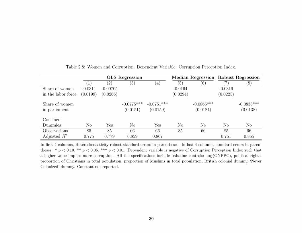
Table 2.8: Women and Corruption. Dependent Variable: Corruption Perception Index.
OLS Regression Median Regression Robust Regression(1) (2) (3) (4) (5) (6) (7) (8)
Share of women -0.0311 -0.00705 -0.0164 -0.0319in the labor force (0.0199) (0.0266) (0.0294) (0.0225)
Share of women -0.0775*** -0.0751*** -0.0865*** -0.0838***in parliament (0.0151) (0.0159) (0.0184) (0.0138)
ContinentDummies No Yes No Yes No No No NoObservations 85 85 66 66 85 66 85 66Adjusted R2 0.775 0.779 0.859 0.867 0.751 0.865
In first 4 columns, Heteroskedasticity-robust standard errors in parentheses. In last 4 columns, standard errors in paren-
theses. * p < 0.10, ** p < 0.05, *** p < 0.01. Dependent variable is negative of Corruption Perception Index such that
a higher value implies more corruption. All the specifications include balseline controls: log (GNPPC), political rights,
proportion of Christians in total population, proportion of Muslims in total population, British colonial dummy, ‘Never
Colonized’ dummy. Constant not reported.
393939
Ordered-probit estimation
Though the corruption indices used in this chapter are continuous variables they are
bounded. Consequently the linear relationship estimated by ordinary least squares (OLS)
may not be most appropriate in this context. Most of the papers in corruption literature,
however, use OLS following the fact that corruption index is a continuous variable and not
an ordering. Brunetti and Weder (2003) argue that OLS is an appropriate specification
and perform ordered-probit regression only as sensitivity check. Note that the corruption
index used by them takes discrete values, and hence, it could be argued that their dependent
variable could be construed as an ordering.25 On the other hand, the index we use is
continuous and does not allow for such criticisms. Nevertheless, we check the sensitivity of
our results using order-probit.
We divide our sample of countries in to 4 categories: very clean (category 1), clean (cat-
egory 2), corrupt (category 3) and highly corrupt (category 4).26 We assign these categories
in the following manner. First, we divide countries in two groups – below mean i.e. below
zero (relatively less corrupt countries), and above mean (relative more corrupt countries).
Next we divide these groups into two sub-groups where there is a natural break in data
points. Table 2.9 describes the assignment of categories and dummies, and the number of
countries that fall under each category. We then perform an ordered-probit regression with
the corruption variable defined as an ordering. In this context, ordered-probit estimation
ensures that the corruption index does not exceed the maximum possible value (i.e. 2.5)
for any country, when the variable of interest (such as the share of women in parliament) is
very large. The results are presented in panel 1 of the Table 2.10. The results are similar
to those obtained using OLS specifications – while the share of women in the labor force is
25The primary measure of corruption used by Brunetti and Weder (2003) is an indicator of corruptionproduced by the International Country Risk Guide (ICRG) that takes only discrete values in the range of0 to 6. They use the average of the index, and use OLS specification. They argue that since corruptionindices are based on numerical ratings and not on country ratings, corruption indices do not actually showthe ordering (or ranking) of a country. See Brunetti and Weder (2003) for detailed discussion on why OLSis the most appropriate specification.
26There could be several other possible ways to define the ordering. We did check the robustness of theresults under other classifications such as dividing the countries in 4 quartiles and found the similar results.
40
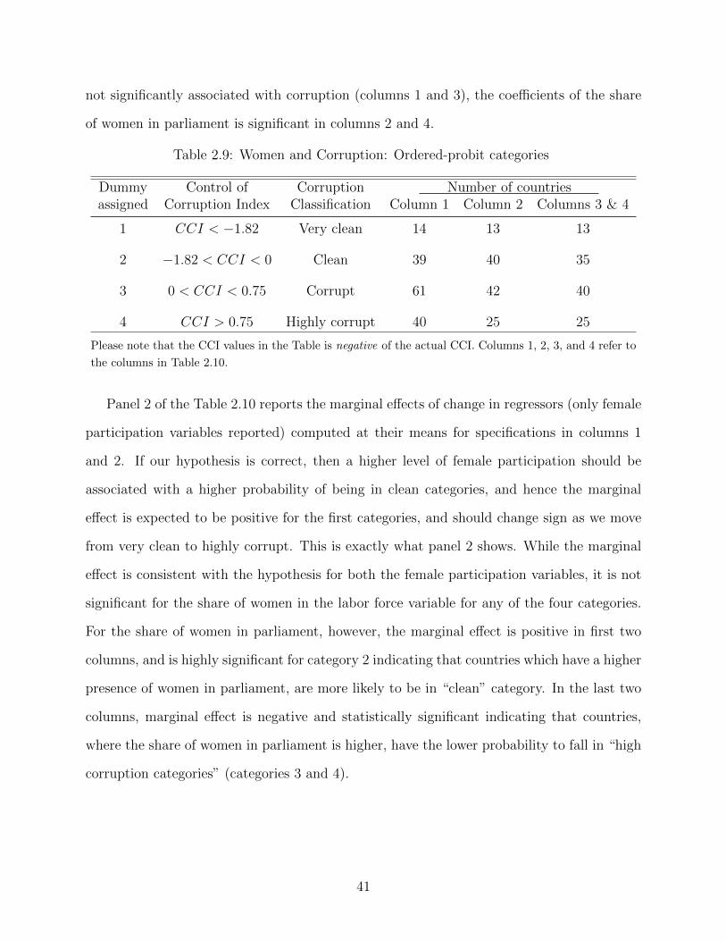
not significantly associated with corruption (columns 1 and 3), the coefficients of the share
of women in parliament is significant in columns 2 and 4.
Table 2.9: Women and Corruption: Ordered-probit categories
Dummy Control of Corruption Number of countriesassigned Corruption Index Classification Column 1 Column 2 Columns 3 & 4
1 CCI < −1.82 Very clean 14 13 13
2 −1.82 < CCI < 0 Clean 39 40 35
3 0 < CCI < 0.75 Corrupt 61 42 40
4 CCI > 0.75 Highly corrupt 40 25 25
Please note that the CCI values in the Table is negative of the actual CCI. Columns 1, 2, 3, and 4 refer to
the columns in Table 2.10.
Panel 2 of the Table 2.10 reports the marginal effects of change in regressors (only female
participation variables reported) computed at their means for specifications in columns 1
and 2. If our hypothesis is correct, then a higher level of female participation should be
associated with a higher probability of being in clean categories, and hence the marginal
effect is expected to be positive for the first categories, and should change sign as we move
from very clean to highly corrupt. This is exactly what panel 2 shows. While the marginal
effect is consistent with the hypothesis for both the female participation variables, it is not
significant for the share of women in the labor force variable for any of the four categories.
For the share of women in parliament, however, the marginal effect is positive in first two
columns, and is highly significant for category 2 indicating that countries which have a higher
presence of women in parliament, are more likely to be in “clean” category. In the last two
columns, marginal effect is negative and statistically significant indicating that countries,
where the share of women in parliament is higher, have the lower probability to fall in “high
corruption categories” (categories 3 and 4).
41
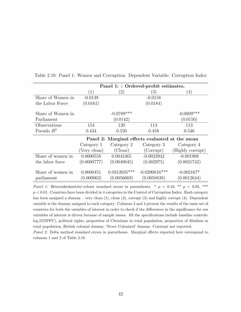
Table 2.10: Panel 1: Women and Corruption. Dependent Variable: Corruption Index
Panel 1: : Ordered-probit estimates.(1) (2) (3) (4)
Share of Women in -0.0139 -0.0158the Labor Force (0.0161) (0.0184)
Share of Women in -0.0789*** -0.0809***Parliament (0.0142) (0.0150)Observations 154 120 113 113Pseudo R2 0.434 0.550 0.458 0.546
Panel 2: Marginal effects evaluated at the meanCategory 1 Category 2 Category 3 Category 4(Very clean) (Clean) (Corrupt) (Highly corrupt)
Share of women in 0.0000558 0.0042465 -0.0023942 -0.001908the labor force (0.0000777) (0.0049845) (0.002975) (0.0021742)
Share of women in 0.0000451 0.0312035*** -0.0290816*** -0.002167*parliament (0.000063) (0.0056669) (0.0058838) (0.0012644)
Panel 1: Heteroskedasticity-robust standard errors in parentheses. * p < 0.10, ** p < 0.05, ***
p < 0.01. Countries have been divided in 4 catogeries in the Control of Corruption Index. Each category
has been assigned a dummy – very clean (1), clean (2), corrupt (3) and highly corrupt (4). Dependent
variable is the dummy assigned to each category. Columns 3 and 4 present the results of the same set of
countries for both the variables of interest in order to check if the differences in the significance for our
variables of interest is driven because of sample issues. All the specifications include baseline controls:
log (GNPPC), political rights, proportion of Christians in total population, proportion of Muslims in
total population, British colonial dummy, ‘Never Colonized’ dummy. Constant not reported.
Panel 2: Delta method standard errors in parentheses. Marginal effects reported here correspond to
columns 1 and 2 of Table 2.10
42
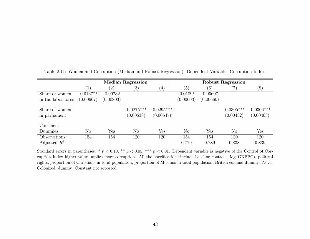
Table 2.11: Women and Corruption (Median and Robust Regression). Dependent Variable: Corruption Index.
Median Regression Robust Regression(1) (2) (3) (4) (5) (6) (7) (8)
Share of women -0.0137** -0.00732 -0.0109* -0.00607in the labor force (0.00667) (0.00803) (0.00603) (0.00660)
Share of women -0.0275*** -0.0295*** -0.0305*** -0.0306***in parliament (0.00538) (0.00647) (0.00432) (0.00463)
ContinentDummies No Yes No Yes No Yes No YesObservations 154 154 120 120 154 154 120 120Adjusted R2 0.779 0.789 0.838 0.839
Standard errors in parentheses. * p < 0.10, ** p < 0.05, *** p < 0.01. Dependent variable is negative of the Control of Cor-
ruption Index higher value implies more corruption. All the specifications include baseline controls: log (GNPPC), political
rights, proportion of Christians in total population, proportion of Muslims in total population, British colonial dummy, ‘Never
Colonized’ dummy. Constant not reported.
434343
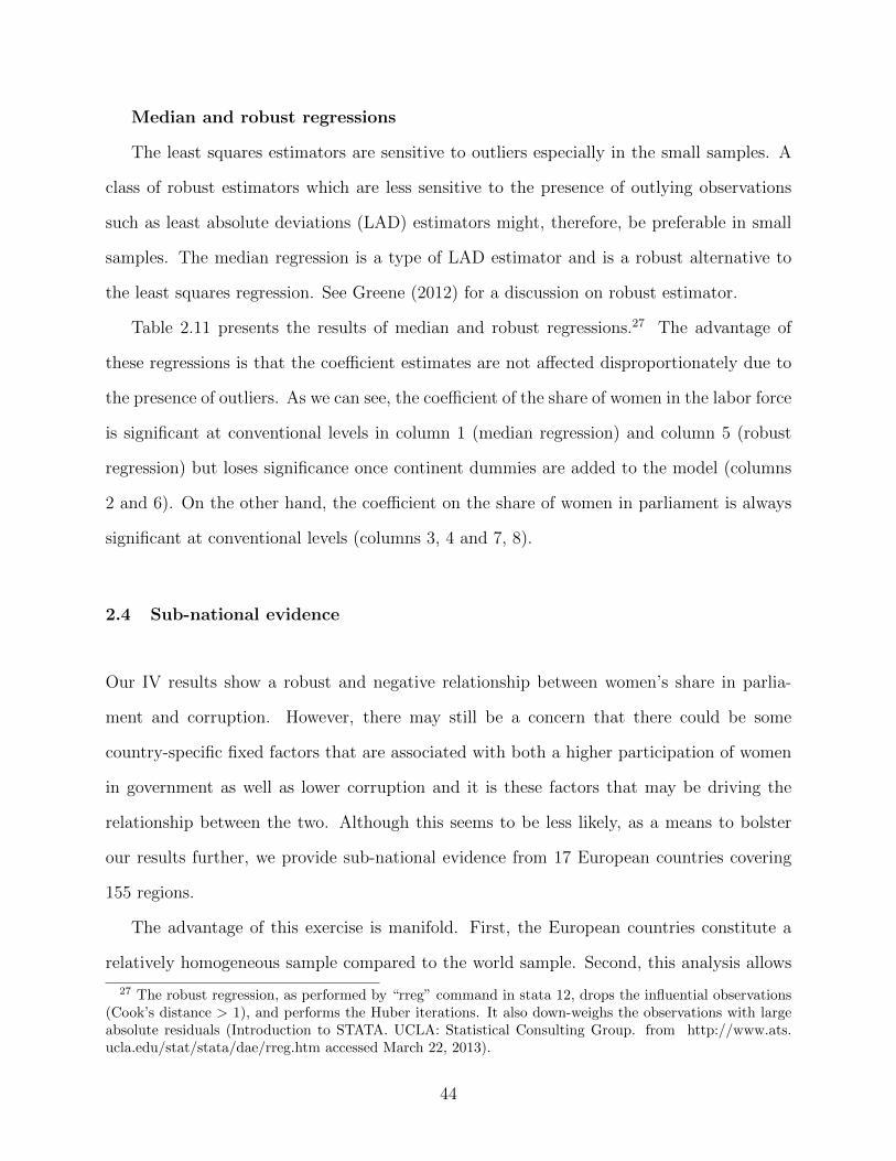
Median and robust regressions
The least squares estimators are sensitive to outliers especially in the small samples. A
class of robust estimators which are less sensitive to the presence of outlying observations
such as least absolute deviations (LAD) estimators might, therefore, be preferable in small
samples. The median regression is a type of LAD estimator and is a robust alternative to
the least squares regression. See Greene (2012) for a discussion on robust estimator.
Table 2.11 presents the results of median and robust regressions.27 The advantage of
these regressions is that the coefficient estimates are not affected disproportionately due to
the presence of outliers. As we can see, the coefficient of the share of women in the labor force
is significant at conventional levels in column 1 (median regression) and column 5 (robust
regression) but loses significance once continent dummies are added to the model (columns
2 and 6). On the other hand, the coefficient on the share of women in parliament is always
significant at conventional levels (columns 3, 4 and 7, 8).
2.4 Sub-national evidence
Our IV results show a robust and negative relationship between women’s share in parlia-
ment and corruption. However, there may still be a concern that there could be some
country-specific fixed factors that are associated with both a higher participation of women
in government as well as lower corruption and it is these factors that may be driving the
relationship between the two. Although this seems to be less likely, as a means to bolster
our results further, we provide sub-national evidence from 17 European countries covering
155 regions.
The advantage of this exercise is manifold. First, the European countries constitute a
relatively homogeneous sample compared to the world sample. Second, this analysis allows
27 The robust regression, as performed by “rreg” command in stata 12, drops the influential observations(Cook’s distance > 1), and performs the Huber iterations. It also down-weighs the observations with largeabsolute residuals (Introduction to STATA. UCLA: Statistical Consulting Group. from http://www.ats.ucla.edu/stat/stata/dae/rreg.htm accessed March 22, 2013).
44
us to control for the country fixed effects ruling out the possibility that our results are
driven by the omission of country fixed factors. Finally, the measure of corruption used
in this exercise is actual corruption instead of perceived corruption and hence is free from
the criticisms that perception indices are subjected to. The corruption or bribery data
comes from the European Quality of Government Index (EQI).28 The first round of the
EQI survey was conducted in 2010 covering 172 regions of 28 member states of European
Union and surveyed 34,000 citizen respondents in December 2009 (Charron et al., 2011).
Our corruption measure is the response to the following question of the 2010 EQI survey:
In the past 12 months have you or anyone living in your household paid a
bribe in any form to:
1. Education services?
2. Health or medical services?
3. Police?
4. Any other government-run agency?
The response “yes” is coded as 1 and “no” is coded as 2, and the percentage of popu-
lation having paid a bribe is calculated. This number is then standardized with the mean
0 and standard deviation 1 such that a higher value indicates lower bribe experience. We
use the negative of the index such that a higher value implies a greater bribery experi-
ence. Sundstrom (2013) has collected data on women’s political representation at the lowest
administrative tier. The unit of analysis in this section is NUTS 2 (the Nomenclature of
Territorial Units for Statistics) – a standard developed by the European Union for subdivi-
sions of countries for statistical purposes. Data for the regional controls by NUTS 2 region
(income per capita, the share of women in the labor force, and proportion of the population
aged 25-64 with tertiary education attainment) are from Eurostat. Table 2.12 provides the
results of the European regional analysis.
28 The EQI data (2013) has been used by some of the recent studies to explore gender differences (forexample, Agerberg, 2014) and the association between corruption and women’s participation in politics(Sundstrom and Wangnerud, 2014).
45
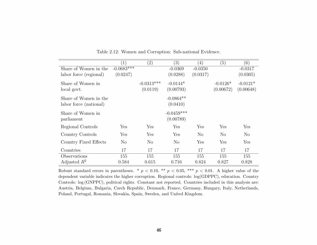
Table 2.12: Women and Corruption: Sub-national Evidence.
(1) (2) (3) (4) (5) (6)Share of Women in the -0.0683*** -0.0369 -0.0350 -0.0317labor force (regional) (0.0247) (0.0288) (0.0317) (0.0305)
Share of Women in -0.0313*** -0.0144* -0.0126* -0.0121*local govt. (0.0119) (0.00793) (0.00672) (0.00648)
Share of Women in the -0.0864**labor force (national) (0.0410)
Share of Women in -0.0459***parliament (0.00789)
Regional Controls Yes Yes Yes Yes Yes Yes
Country Controls Yes Yes Yes No No No
Country Fixed Effects No No No Yes Yes Yes
Countries 17 17 17 17 17 17Observations 155 155 155 155 155 155Adjusted R2 0.584 0.615 0.716 0.824 0.827 0.828
Robust standard errors in parentheses. * p < 0.10, ** p < 0.05, *** p < 0.01. A higher value of the
dependent variable indicates the higher corruption. Regional controls: log(GDPPC), education. Country
Controls: log (GNPPC), political rights. Constant not reported. Countries included in this analysis are:
Austria, Belgium, Bulgaria, Czech Republic, Denmark, France, Germany, Hungary, Italy, Netherlands,
Poland, Portugal, Romania, Slovakia, Spain, Sweden, and United Kingdom.
464646
In the first 3 columns of Table 2.12, instead of controlling for the country fixed effects,
we control for country-level variables – income and political rights along with the regional
variables – income levels and the education. In the first two columns, a higher share of women
in the labor force and a higher share of women in local government are found to be negatively
associated with bribe experiences of citizens. Column 3 controls for the share of women in
parliament and the national share of women in the labor force. While women’s participation
in politics at both levels, local and national, is associated with lower corruption, only women’s
share in the national labor force is found to have a negative association with corruption.
The results, however, may have been driven by the omission of the country fixed factors.
In order to rule out this possibility, we include continent dummies in the next 3 columns.
While the share of women in local government is still negatively associated with corruption,
the association between the share of women in the labor force and corruption disappears
once country fixed factors are controlled for. Our analysis of 17 European countries, thus,
suggests that the effect of women’s presence in politics on corruption is not driven by country-
specific fixed factors and that the relationship between the women’s political participation
and corruption is indeed causal.
2.5 Will the relationship between gender and corruption disappear as womenbecome more equal?
In this section, we explore the notion of “corruption convergence in gender”, that is,
whether women’s participation in corrupt activities will be no different from that of men as
they become similar to men in their social status. This could be one possible explanation
since none of the previous studies claim that women are inherently less corrupt or that
the observed gender differences in attitude towards corruption are permanent or biological.
Ideally, this issue should be investigated using a panel specification, but as mentioned earlier,
this is not feasible when using corruption indices. Hence, we devise an alternative approach
to deal with this problem.
47
As discussed in the introduction, several studies have suggested that the observed gender
differences in attitude towards corruption could be the result of gender differences in social
status or women’s lack of knowledge regarding how to engage in corrupt activities or their
ability to make decisions relating to corrupt activities or even for that matter being given
access to corrupt activities. For instance, Goetz (2007) gives the example of Peru where the
salary of traffic cops is insufficient to maintain a family. She observes that while men as
traffic officers accept bribes, this is not yet the case for women. However, doubting that this
will persist in the long run, she writes “...women will not passively conform to the idealized
notions of their finer moral nature when they have families to feed and if there is money to
be made from public office.”
Consequently, one possibility is that there would be no difference in corrupt behavior
between men and women if women held similar status as men. We capture this issue by
using the Gender Inequality Index (GII) computed by the United Nations Development Pro-
gramme (UNDP) as a measure of the status difference between genders. The index can
take a value in the range of 0 (implying more equal gender-status) to 1 (when gender-gap is
large). The GII is calculated by the United Nations Development Programme (UNDP). It
is a broader measure of gender-gap than educational attainment gap, or life expectancy gap
across genders. According to UNDP “the Gender Inequality Index is designed to reveal the
extent to which national achievements in these aspects [reproductive health, empowerment
and the labor market] of human development are eroded by gender inequality, and to provide
empirical foundations for policy analysis and advocacy efforts.” The health dimension con-
trols for the maternal mortality rate and the adolescent fertility rate. Essentially there are
no male-equivalent indicators for reproductive health, as a result the ideal social goals – no
maternal death and no adolescent pregnancy, are taken as comparison points. The secondary
and higher educational attainment, and the share of each sex in parliament is included in
the empowerment dimension. Women’s participation in the work force is used as a measure
48
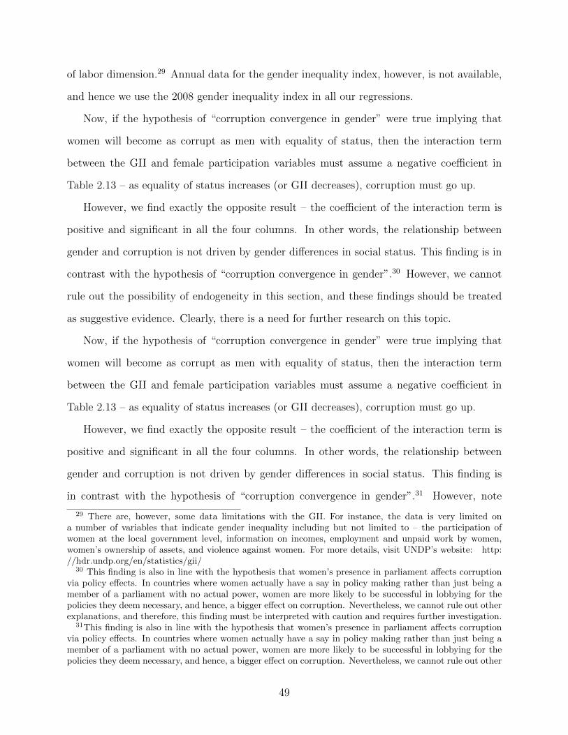
of labor dimension.29 Annual data for the gender inequality index, however, is not available,
and hence we use the 2008 gender inequality index in all our regressions.
Now, if the hypothesis of “corruption convergence in gender” were true implying that
women will become as corrupt as men with equality of status, then the interaction term
between the GII and female participation variables must assume a negative coefficient in
Table 2.13 – as equality of status increases (or GII decreases), corruption must go up.
However, we find exactly the opposite result – the coefficient of the interaction term is
positive and significant in all the four columns. In other words, the relationship between
gender and corruption is not driven by gender differences in social status. This finding is in
contrast with the hypothesis of “corruption convergence in gender”.30 However, we cannot
rule out the possibility of endogeneity in this section, and these findings should be treated
as suggestive evidence. Clearly, there is a need for further research on this topic.
Now, if the hypothesis of “corruption convergence in gender” were true implying that
women will become as corrupt as men with equality of status, then the interaction term
between the GII and female participation variables must assume a negative coefficient in
Table 2.13 – as equality of status increases (or GII decreases), corruption must go up.
However, we find exactly the opposite result – the coefficient of the interaction term is
positive and significant in all the four columns. In other words, the relationship between
gender and corruption is not driven by gender differences in social status. This finding is
in contrast with the hypothesis of “corruption convergence in gender”.31 However, note
29 There are, however, some data limitations with the GII. For instance, the data is very limited ona number of variables that indicate gender inequality including but not limited to – the participation ofwomen at the local government level, information on incomes, employment and unpaid work by women,women’s ownership of assets, and violence against women. For more details, visit UNDP’s website: http://hdr.undp.org/en/statistics/gii/
30 This finding is also in line with the hypothesis that women’s presence in parliament affects corruptionvia policy effects. In countries where women actually have a say in policy making rather than just being amember of a parliament with no actual power, women are more likely to be successful in lobbying for thepolicies they deem necessary, and hence, a bigger effect on corruption. Nevertheless, we cannot rule out otherexplanations, and therefore, this finding must be interpreted with caution and requires further investigation.
31This finding is also in line with the hypothesis that women’s presence in parliament affects corruptionvia policy effects. In countries where women actually have a say in policy making rather than just being amember of a parliament with no actual power, women are more likely to be successful in lobbying for thepolicies they deem necessary, and hence, a bigger effect on corruption. Nevertheless, we cannot rule out other
49
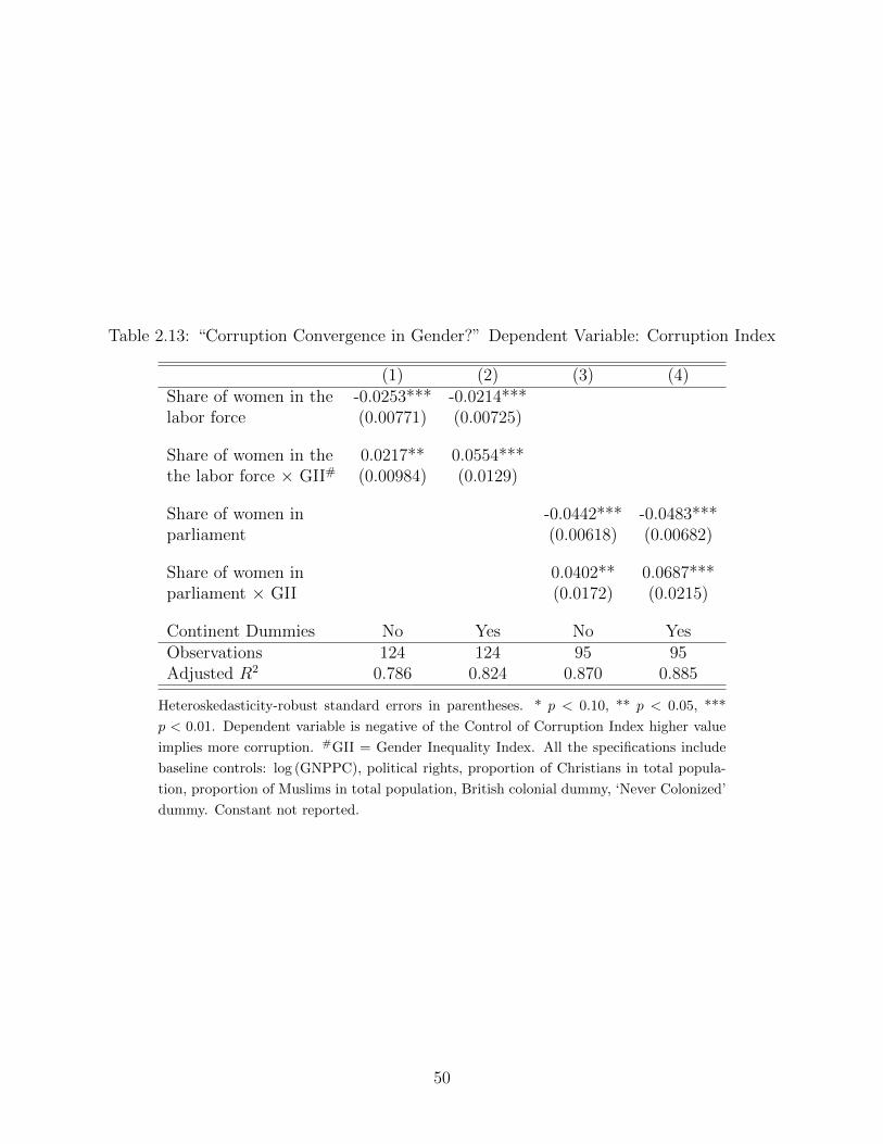
Table 2.13: “Corruption Convergence in Gender?” Dependent Variable: Corruption Index
(1) (2) (3) (4)Share of women in the -0.0253*** -0.0214***labor force (0.00771) (0.00725)
Share of women in the 0.0217** 0.0554***the labor force × GII# (0.00984) (0.0129)
Share of women in -0.0442*** -0.0483***parliament (0.00618) (0.00682)
Share of women in 0.0402** 0.0687***parliament × GII (0.0172) (0.0215)
Continent Dummies No Yes No YesObservations 124 124 95 95Adjusted R2 0.786 0.824 0.870 0.885
Heteroskedasticity-robust standard errors in parentheses. * p < 0.10, ** p < 0.05, ***
p < 0.01. Dependent variable is negative of the Control of Corruption Index higher value
implies more corruption. #GII = Gender Inequality Index. All the specifications include
baseline controls: log (GNPPC), political rights, proportion of Christians in total popula-
tion, proportion of Muslims in total population, British colonial dummy, ‘Never Colonized’
dummy. Constant not reported.
50
that we cannot rule out the possibility of endogeneity in this section, and these findings are
just suggestive evidence – an acceptance or rejection of this hypothesis calls for the need of
further research.
2.6 Concluding remarks
In investigating the role in which women can affect corruption, this chapter finds that
women’s presence in the labor force, in clerical positions, and in decision-making (senior-
level) positions is not significantly associated with corruption in a country. We show that
women are able to have a systematic negative impact on corruption only if they are repre-
sented in parliaments and possibly through policy making. We use instruments to establish
causality, and draw inferences based on the conditional likelihood ratio approach proposed by
Moreira (2003), Anderson-Rubin Statistic (Anderson and Rubin, 1949), and LM−J statistic
(Kleibergen, 2002). Our results are also shown to hold in a regional analysis of European
countries where after controlling for the country fixed effects, we find that women’s share in
the local government is associated with lower bribery. Finally, our results also suggest that
observed gender differences in corruption are not entirely be driven by gender differences in
social status.
Our analysis also raises one question for future research – how do women reduce cor-
ruption by being in politics? One possible answer could be that they favor policies that are
different from those favored by men. The recent literature has extensively explored the policy
implications of gender representation in government. Women in local government in India
have been reported to allocate a greater budget to public goods more closely associated with
women’s concerns (Chattopadhyay and Duflo, 2004), to the provision of basic infrastructural
needs, and to be more concerned about whether the subsidies were provided to the targeted
group without corruption (Kudva, 2003). Moreover, the female political representation has
also been found to be positively associated with the state health spending (Rehavi, 2007) and
explanations, and therefore, this finding must be interpreted with caution and requires further investigation.
51
educational outcomes Clots-Figueras, 2011.32 The political science literature also documents
that women in the government tend to introduce and pass more bills that are concerned with
the welfare of women, children and families (Thomas, 1991), advocate women’s right issues
more strongly than men, and participate more frequently in debates on bills that address
issues of women, children and the family than debates on other bills (Taylor-Robinson and
Heath, 2003).
At the same time, there are also studies which show that education reduces corruption.
For instance, Glaeser and Saks (2006) find that corruption, as measured by “the number of
government officials convicted for corrupt practices through the Federal justice department”,
is less in more educated states in America. Moreover, our findings also refute the hypothesis
that the observed gender differences in the attitude towards corruption is entirely due to
gender differences in social status and will disappear over time when women acquire more
equal socio-economic status. Indeed if women have distinct preferences for policies that
are different from that of men and if policy-making is the channel through which women
in government affect corruption, then there is little reason to think that the association
between women’s presence and corruption will vanish as they get similar as men in social
status. Clearly this question bears further investigation.
To sum up, gender inequality is still persistent around the globe. The gender gap exists
in access to education, work and participation in economic and political activities. In the
Millennium Development Goal Report (2012), United Nations recognizes the importance of
women’s empowerment for achieving its goals. The findings of this chapter suggest that
women’s participation in politics should not only be encouraged for the sake of obtaining
gender equality but also because it has positive externalities – a negative impact on corrup-
tion.
32 Rehavi (2007) finds that the share of women in state houses in the US states is positively associatedwith the state health spending. Clots-Figueras (2011) finds that the probability an individual will attainprimary education in urban areas in India is positively associated with female political representation.
52
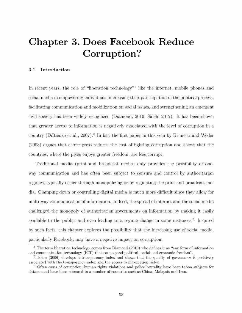
Chapter 3. Does Facebook ReduceCorruption?
3.1 Introduction
In recent years, the role of “liberation technology”1 like the internet, mobile phones and
social media in empowering individuals, increasing their participation in the political process,
facilitating communication and mobilization on social issues, and strengthening an emergent
civil society has been widely recognized (Diamond, 2010; Saleh, 2012). It has been shown
that greater access to information is negatively associated with the level of corruption in a
country (DiRienzo et al., 2007).2 In fact the first paper in this vein by Brunetti and Weder
(2003) argues that a free press reduces the cost of fighting corruption and shows that the
countries, where the press enjoys greater freedom, are less corrupt.
Traditional media (print and broadcast media) only provides the possibility of one-
way communication and has often been subject to censure and control by authoritarian
regimes, typically either through monopolizing or by regulating the print and broadcast me-
dia. Clamping down or controlling digital media is much more difficult since they allow for
multi-way communication of information. Indeed, the spread of internet and the social media
challenged the monopoly of authoritarian governments on information by making it easily
available to the public, and even leading to a regime change in some instances.3 Inspired
by such facts, this chapter explores the possibility that the increasing use of social media,
particularly Facebook, may have a negative impact on corruption.
1 The term liberation technology comes from Diamond (2010) who defines it as “any form of informationand communication technology (ICT) that can expand political, social and economic freedom”.
2 Islam (2006) develops a transparency index and shows that the quality of governance is positivelyassociated with the transparency index and the access to information index.
3 Often cases of corruption, human rights violations and police brutality have been taboo subjects forcitizens and have been censored in a number of countries such as China, Malaysia and Iran.
53
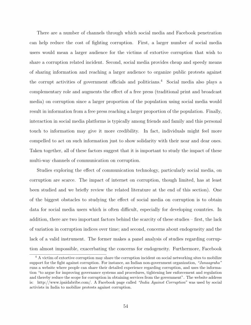
There are a number of channels through which social media and Facebook penetration
can help reduce the cost of fighting corruption. First, a larger number of social media
users would mean a larger audience for the victims of extortive corruption that wish to
share a corruption related incident. Second, social media provides cheap and speedy means
of sharing information and reaching a larger audience to organize public protests against
the corrupt activities of government officials and politicians.4 Social media also plays a
complementary role and augments the effect of a free press (traditional print and broadcast
media) on corruption since a larger proportion of the population using social media would
result in information from a free press reaching a larger proportion of the population. Finally,
interaction in social media platforms is typically among friends and family and this personal
touch to information may give it more credibility. In fact, individuals might feel more
compelled to act on such information just to show solidarity with their near and dear ones.
Taken together, all of these factors suggest that it is important to study the impact of these
multi-way channels of communication on corruption.
Studies exploring the effect of communication technology, particularly social media, on
corruption are scarce. The impact of internet on corruption, though limited, has at least
been studied and we briefly review the related literature at the end of this section). One
of the biggest obstacles to studying the effect of social media on corruption is to obtain
data for social media users which is often difficult, especially for developing countries. In
addition, there are two important factors behind the scarcity of these studies – first, the lack
of variation in corruption indices over time; and second, concerns about endogeneity and the
lack of a valid instrument. The former makes a panel analysis of studies regarding corrup-
tion almost impossible, exacerbating the concerns for endogeneity. Furthermore, Facebook
4 A victim of extortive corruption may share the corruption incident on social networking sites to mobilizesupport for the fight against corruption. For instance, an Indian non-government organization, “Janaagraha”runs a website where people can share their detailed experience regarding corruption, and uses the informa-tion “to argue for improving governance systems and procedures, tightening law enforcement and regulationand thereby reduce the scope for corruption in obtaining services from the government”. The website addressis: http://www.ipaidabribe.com/. A Facebook page called “India Against Corruption” was used by socialactivists in India to mobilize protests against corruption.
54
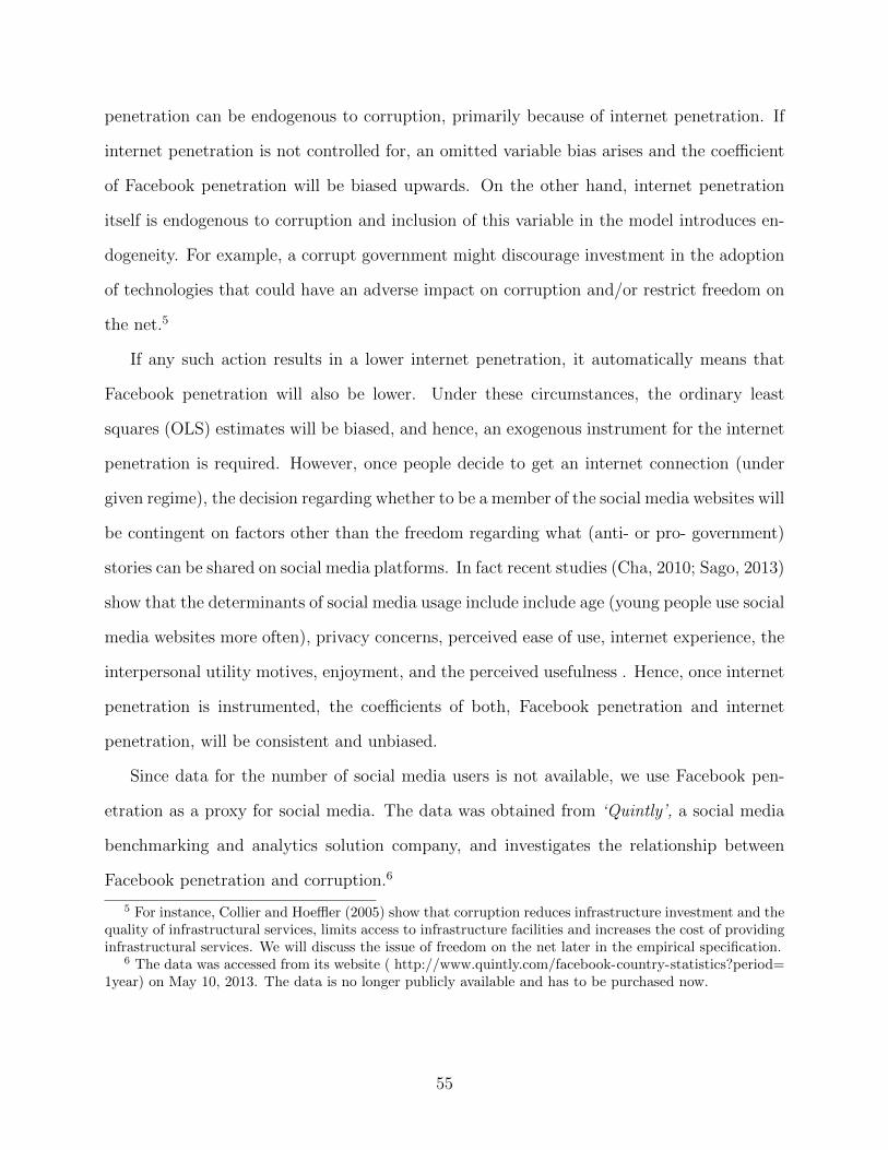
penetration can be endogenous to corruption, primarily because of internet penetration. If
internet penetration is not controlled for, an omitted variable bias arises and the coefficient
of Facebook penetration will be biased upwards. On the other hand, internet penetration
itself is endogenous to corruption and inclusion of this variable in the model introduces en-
dogeneity. For example, a corrupt government might discourage investment in the adoption
of technologies that could have an adverse impact on corruption and/or restrict freedom on
the net.5
If any such action results in a lower internet penetration, it automatically means that
Facebook penetration will also be lower. Under these circumstances, the ordinary least
squares (OLS) estimates will be biased, and hence, an exogenous instrument for the internet
penetration is required. However, once people decide to get an internet connection (under
given regime), the decision regarding whether to be a member of the social media websites will
be contingent on factors other than the freedom regarding what (anti- or pro- government)
stories can be shared on social media platforms. In fact recent studies (Cha, 2010; Sago, 2013)
show that the determinants of social media usage include include age (young people use social
media websites more often), privacy concerns, perceived ease of use, internet experience, the
interpersonal utility motives, enjoyment, and the perceived usefulness . Hence, once internet
penetration is instrumented, the coefficients of both, Facebook penetration and internet
penetration, will be consistent and unbiased.
Since data for the number of social media users is not available, we use Facebook pen-
etration as a proxy for social media. The data was obtained from ‘Quintly’, a social media
benchmarking and analytics solution company, and investigates the relationship between
Facebook penetration and corruption.6
5 For instance, Collier and Hoeffler (2005) show that corruption reduces infrastructure investment and thequality of infrastructural services, limits access to infrastructure facilities and increases the cost of providinginfrastructural services. We will discuss the issue of freedom on the net later in the empirical specification.
6 The data was accessed from its website ( http://www.quintly.com/facebook-country-statistics?period=1year) on May 10, 2013. The data is no longer publicly available and has to be purchased now.
55
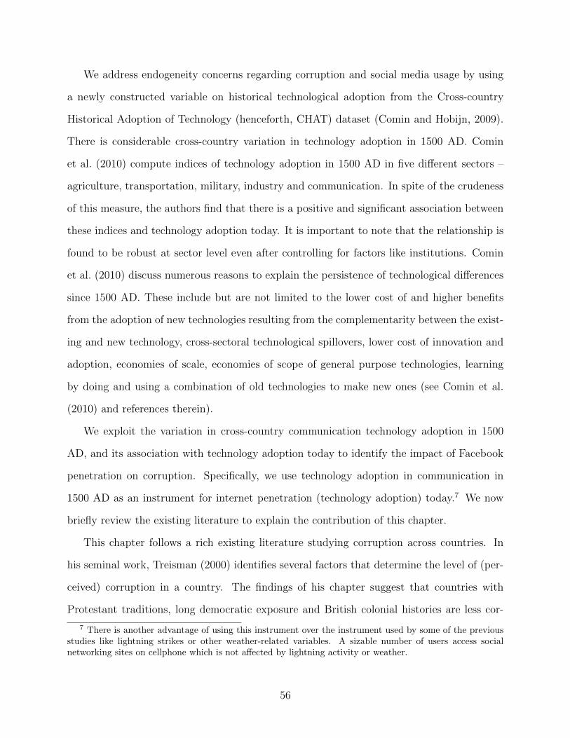
We address endogeneity concerns regarding corruption and social media usage by using
a newly constructed variable on historical technological adoption from the Cross-country
Historical Adoption of Technology (henceforth, CHAT) dataset (Comin and Hobijn, 2009).
There is considerable cross-country variation in technology adoption in 1500 AD. Comin
et al. (2010) compute indices of technology adoption in 1500 AD in five different sectors –
agriculture, transportation, military, industry and communication. In spite of the crudeness
of this measure, the authors find that there is a positive and significant association between
these indices and technology adoption today. It is important to note that the relationship is
found to be robust at sector level even after controlling for factors like institutions. Comin
et al. (2010) discuss numerous reasons to explain the persistence of technological differences
since 1500 AD. These include but are not limited to the lower cost of and higher benefits
from the adoption of new technologies resulting from the complementarity between the exist-
ing and new technology, cross-sectoral technological spillovers, lower cost of innovation and
adoption, economies of scale, economies of scope of general purpose technologies, learning
by doing and using a combination of old technologies to make new ones (see Comin et al.
(2010) and references therein).
We exploit the variation in cross-country communication technology adoption in 1500
AD, and its association with technology adoption today to identify the impact of Facebook
penetration on corruption. Specifically, we use technology adoption in communication in
1500 AD as an instrument for internet penetration (technology adoption) today.7 We now
briefly review the existing literature to explain the contribution of this chapter.
This chapter follows a rich existing literature studying corruption across countries. In
his seminal work, Treisman (2000) identifies several factors that determine the level of (per-
ceived) corruption in a country. The findings of his chapter suggest that countries with
Protestant traditions, long democratic exposure and British colonial histories are less cor-
7 There is another advantage of using this instrument over the instrument used by some of the previousstudies like lightning strikes or other weather-related variables. A sizable number of users access socialnetworking sites on cellphone which is not affected by lightning activity or weather.
56

rupt. In another significant paper, Brunetti and Weder (2003) investigate the impact of
the press freedom on corruption. They classify press freedom as an external mechanism to
control corruption – a control exercised by individuals or organizations that are outsiders
to the network of corruption, i.e. the bureaucratic system. They argue that press freedom
puts a check on corruption by reducing the cost of fighting corruption.8 Using Hausman and
Taylor’s technique, Elbahnasawy and Revier (2012) study the effect of both, time-variant
and time-invariant factors on corruption and find that while the rule of law, perception of
free expression and accountability, and free media reduce corruption, factors such as natural
resource abundance, religious tradition, political stability, and ethnic fractionalization do
not matter for corruption.
Goel et al. (2012) show that greater internet awareness regarding corruption is associated
with lower corruption across countries using internet searches for corruption (such as “cor-
ruption”, “bribery” and “country name”) on Google and Yahoo as the measure of internet
awareness. Andersen et al. (2011), using lightning activity as an instrument for internet
diffusion, show that internet penetration is negatively related to corruption. Using dynamic
panel data model to address endogeneity concerns, Elbahnasawy (2014) finds that a greater
use of e-government and greater internet adoption are associated with lower corruption.9
Continuing in this vein, the present chapter explores the impact of Facebook on corruption.
To the best of our knowledge, this chapter is the first comprehensive study to quantify the
impact of social media on corruption.
Our results show that Facebook penetration has a causal and negative impact on cor-
ruption. We address the endogeneity concerns by instrumenting internet penetration with
the 1500 technology adoption in the field of communication. We show that our instrument
8 According to Brunetti and Weder a free press is especially more effective in fighting collusive corruptionwhere the internal controls of corruption – the agencies that control corruption within bureaucracy – arelikely to be less effective. See Brunetti and Weder (2003) for an excellent discussion of the two kinds ofcorruption and how a free press is an effective tool against these kinds of corruption.
9 An important caveat of this study must be kept in mind while interpreting the results. TransparencyInternational, the publisher of Corruption Perception Index, the corruption measure used in this study, warnsthat these indices are not comparable across time prior to 2012. See http://www.transparency.org/files/content/pressrelease/2012 CPIUpdatedMethodology EMBARGO EN.pdf for details.
57

is strong even when we control for a number of institutional, cultural, historical, and con-
temporary variables that might potentially be correlated with past and present levels of
corruption and/or past and current levels of technology adoption. Moreover, we perform
a variety of robustness checks on Facebook-corruption relationship including a falsification
test that confirms that this relationship is causal. We find that while there is no association
between Facebook penetration and corruption index prior to the launch of Facebook, there
is a mild association between Facebook penetration and corruption index 2 years after Face-
book was introduced and that this association becomes much stronger in 2011 (8 years after
the inception of the Facebook). Consistent with the findings of the previous studies, we also
find that internet penetration is negatively related with corruption.
The rest of the chapter is organized as follows. In the next section, we briefly describe our
data sources. Section 3 outlines the empirical strategy. In sections 4, we present OLS and IV
results. Section 5 presents robustness checks and falsification test of the Facebook-corruption
relationship and section 6 concludes.
3.2 Data and empirical strategy
3.2.1 Data
This chapter uses the 2011 Control of Corruption Index (CCI) published by the World Bank
as the primary measure of corruption (Corruption).10 Kaufmann et al. (2011) describe the
objective of the CCI as – “capturing perceptions of the extent to which public power is
exercised for private gain, including both petty and grand forms of corruption, as well as
“capture” of the state by elites and private interests.” The CCI takes values in the range of
−2.5 to 2.5, with−2.5 representing the most severe corruption and 2.5 representing the lowest
10 The results are robust to the use of an alternative measure of corruption – the 2011 Corruption Percep-tion Index published by Transparency International that defines corruption as “the misuse of public powerfor private benefit”.
58
level of corruption.11 The data source for our variable of interest, Facebook penetration, is
Quintly, a social media benchmarking and analytics solution company. ‘Quintly’ uses the
Facebook advertising tool in order to collect data on Facebook users in different countries.
Even though the advertising tool belongs to Facebook, Quintly data has to be interpreted
carefully since Facebook claims that these data are not completely accurate. The official
number of Facebook users may be slightly different from the number of Facebook users
indicated by this advertising tool. For example, Facebook reported 1.11 billion users at the
end of March, 2013 while the number of users reported by the advertising data was 965
million, or a difference of roughly 13 percent indicating that “[this] advertising data can be
seen as rough estimates for the Facebook country statistics. No more, no less.” (Nierhoff,
2013).
The data source for our instrument is Comin et al. (2010) who use a number of historical
sources of information to compute an index of cross-country technology adoption in 1000
BC, 0 AD, and 1500 AD. They note that 1500 AD data is more precise because of a large
number of sources documenting the technology adoption patterns. Since internet is a part of
communication technology, our instrument is technology adoption in communication. Note
that Comin et al. (2010) take care to ensure that this measure does not incorporate technol-
ogy transferred by Europeans to the rest of the world. The construction of communication
index uses four variables – ‘the use of movable block printing’, ‘the use of woodblock print-
ing’, ‘the use of books’ and ‘the use of paper’. Comin et al. (2010) find that this is a good
predictor of technology adoption today even after controlling for a number of variables like
geographical and institutional factors. This index is created on the basis of the extensive
margin of technology adoption and not the extent to which these technologies were used (i.e.
intensive margin) and takes a value between 0 and 1.12
11 Further details about the CCI can be found in the data section of Chapter 2.12 The construction of this data takes into account the fragmentation and unification of countries subse-
quent to the period to which the data belongs. Interested readers may refer to Comin and Hobijn (2009)and Comin et al. (2010) for the details about the methodology of constructing the index and the sources ofinformation that have been used to construct these indices.
59
We use Gross Domestic Product (GDP) as a measure of income. The data for GDP
per capita (log(GDPPC)) and internet penetration have been taken from the World Bank.
Freedom House publishes data on political rights (Pol Rights) and press freedom (Press).
The political rights index can take a value from 1 through 7, with a lower value representing
better political rights. A very high rating such as 7 would imply that political rights of the
citizens are severely compromised. Such countries may be characterized by severe government
oppression, absence of a functioning central government and widespread extreme violence.
Each country is given a score from 0 to 100 in the press freedom index, with a lower score
implying a freer press. The 2011 press freedom index for a country is determined on the basis
of its performance in three broad categories: the legal, political and economic environment.
The legal environment takes into account the extent to which freedom of expression of
individuals including journalists and bloggers are protected by the law, and the extent of
freedom granted by law to media regulatory bodies. The political environment category
ranks a country on the basis of the following criteria – editorial independence, official and
self-control of state-owned and private media, public access to media coverage, and the ability
of local and foreign journalists to publish news freely and without harassment from agents
of the state or others. Finally, the economic environment consists of the cost associated
with establishing media agencies and government’s control over media, transparency and
concentration of media ownership, and the extent to which journalists and bloggers are
influenced by economic incentives from private or public sources.
Population (log (Population)) data comes from the World Bank. The data for the pro-
portion of population belonging to Christian (Christian) and Muslim (Muslim) faiths in
the total population is obtained from the Association of Religion Data Archive.13 The data
on urban population (Urban) comes from the World Bank and refers to the percentage of
population living in the areas which have been defined as ‘urban’ by the country’s national
statistical office. The World Bank also provides data for the number of cellphone subscribers
13 http://thearda.com. The principal investigators for this data set are the following: Jaime Harris,Robert R. Martin, Sarah Montminy, and Roger Finke of The Association of Religion Data Archive.
60
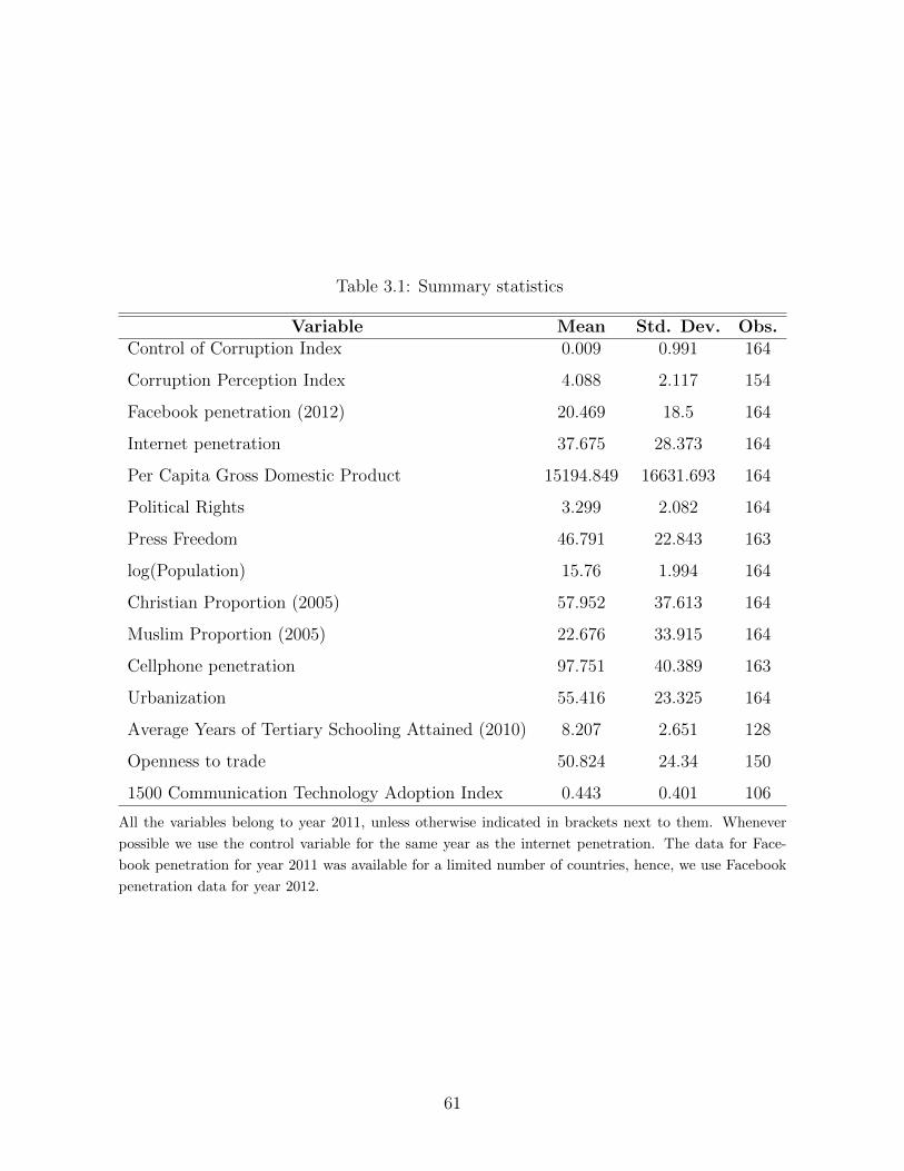
Table 3.1: Summary statistics
Variable Mean Std. Dev. Obs.Control of Corruption Index 0.009 0.991 164
Corruption Perception Index 4.088 2.117 154
Facebook penetration (2012) 20.469 18.5 164
Internet penetration 37.675 28.373 164
Per Capita Gross Domestic Product 15194.849 16631.693 164
Political Rights 3.299 2.082 164
Press Freedom 46.791 22.843 163
log(Population) 15.76 1.994 164
Christian Proportion (2005) 57.952 37.613 164
Muslim Proportion (2005) 22.676 33.915 164
Cellphone penetration 97.751 40.389 163
Urbanization 55.416 23.325 164
Average Years of Tertiary Schooling Attained (2010) 8.207 2.651 128
Openness to trade 50.824 24.34 150
1500 Communication Technology Adoption Index 0.443 0.401 106
All the variables belong to year 2011, unless otherwise indicated in brackets next to them. Whenever
possible we use the control variable for the same year as the internet penetration. The data for Face-
book penetration for year 2011 was available for a limited number of countries, hence, we use Facebook
penetration data for year 2012.
61
per capita. Average years of tertiary schooling attained has been used a measure of educa-
tional attainment for which the data source is Barro and Lee (2013) . The share of imports in
GDP is used as a measure of openness using data from the World Bank. Summary statistics
are presented in Table 3.1.
Figure 3.1 presents the scatter plot of internet penetration and corruption, and Figure 3.2
presents the scatter plot of Facebook penetration and corruption. These figures indicate a
negative association between internet penetration and corruption, and Facebook penetration
and corruption.
3.2.2 Empirical strategy
In order to assess the impact of Facebook penetration on corruption, we estimate the fol-
lowing equation:
Corruptioni = α + β Facebooki + δ Interneti + γ1 log(GDPPCi) + γ2 Political Rightsi
+ γ3 log(Populationi) + γ4Christiani + γ5Muslimi + γ6 Urbani + εi (3.1)
where subscript i denotes the country. Since we use the negative of the corruption index
implying a higher value means higher corruption, β and δ are expected to be negative.
We control for (log of) GDPPC since rich countries can afford to have better institutions
and therefore may be able to control corruption more effectively (Treisman, 2000). As
a result, the coefficient of log(GDPPC) is expected to be negative. Corruption is lower
in countries with long democratic history, parliamentary system, and politically stability
(Treisman, 2000; Lederman et al., 2005; Campante et al., 2009).14 In countries where people
enjoy higher political rights, the press is free and the judiciary is independent, corruption is
14 Campante et al. (2009) find a U-shaped relationship between the corruption perception and several mea-sures of incumbent stability (such as average tenures of chief executives and governing parties): corruptionis greater under very stable and unstable regimes compared to regimes with intermediate stability.
62
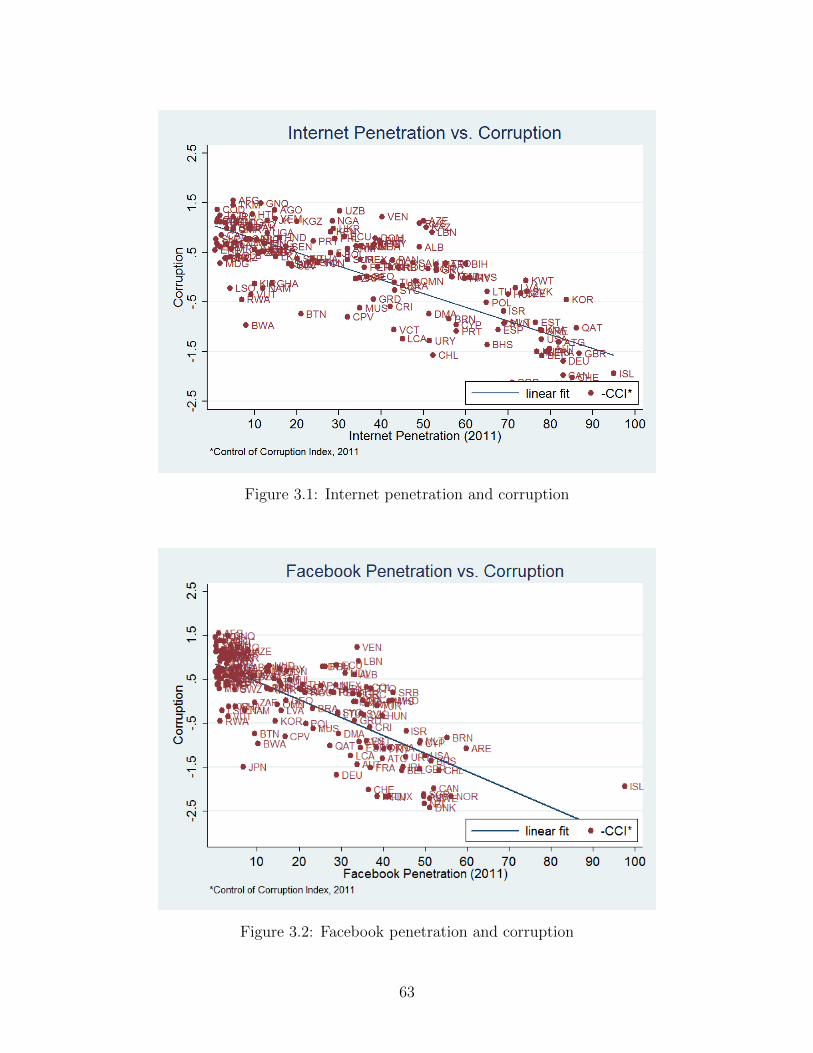
Figure 3.1: Internet penetration and corruption
Figure 3.2: Facebook penetration and corruption
63
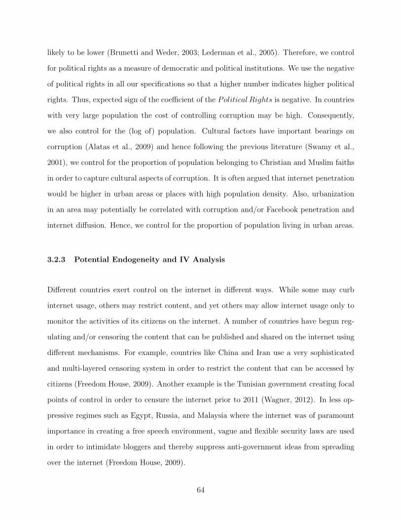
likely to be lower (Brunetti and Weder, 2003; Lederman et al., 2005). Therefore, we control
for political rights as a measure of democratic and political institutions. We use the negative
of political rights in all our specifications so that a higher number indicates higher political
rights. Thus, expected sign of the coefficient of the Political Rights is negative. In countries
with very large population the cost of controlling corruption may be high. Consequently,
we also control for the (log of) population. Cultural factors have important bearings on
corruption (Alatas et al., 2009) and hence following the previous literature (Swamy et al.,
2001), we control for the proportion of population belonging to Christian and Muslim faiths
in order to capture cultural aspects of corruption. It is often argued that internet penetration
would be higher in urban areas or places with high population density. Also, urbanization
in an area may potentially be correlated with corruption and/or Facebook penetration and
internet diffusion. Hence, we control for the proportion of population living in urban areas.
3.2.3 Potential Endogeneity and IV Analysis
Different countries exert control on the internet in different ways. While some may curb
internet usage, others may restrict content, and yet others may allow internet usage only to
monitor the activities of its citizens on the internet. A number of countries have begun reg-
ulating and/or censoring the content that can be published and shared on the internet using
different mechanisms. For example, countries like China and Iran use a very sophisticated
and multi-layered censoring system in order to restrict the content that can be accessed by
citizens (Freedom House, 2009). Another example is the Tunisian government creating focal
points of control in order to censure the internet prior to 2011 (Wagner, 2012). In less op-
pressive regimes such as Egypt, Russia, and Malaysia where the internet was of paramount
importance in creating a free speech environment, vague and flexible security laws are used
in order to intimidate bloggers and thereby suppress anti-government ideas from spreading
over the internet (Freedom House, 2009).
64
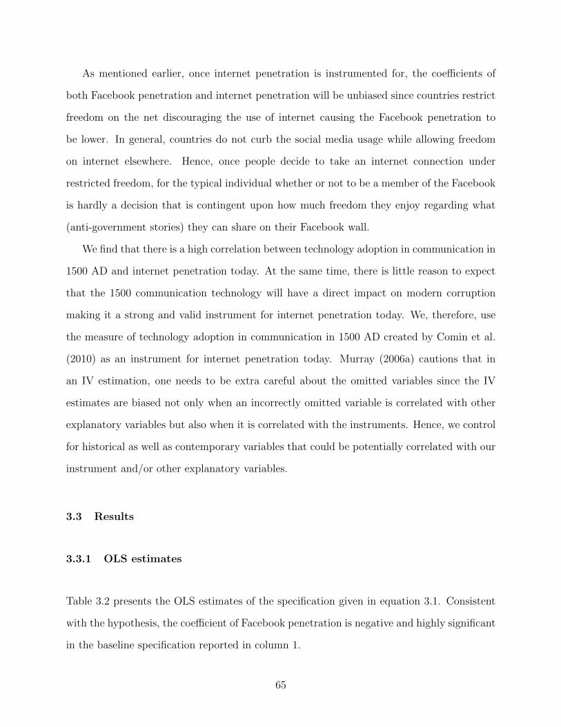
As mentioned earlier, once internet penetration is instrumented for, the coefficients of
both Facebook penetration and internet penetration will be unbiased since countries restrict
freedom on the net discouraging the use of internet causing the Facebook penetration to
be lower. In general, countries do not curb the social media usage while allowing freedom
on internet elsewhere. Hence, once people decide to take an internet connection under
restricted freedom, for the typical individual whether or not to be a member of the Facebook
is hardly a decision that is contingent upon how much freedom they enjoy regarding what
(anti-government stories) they can share on their Facebook wall.
We find that there is a high correlation between technology adoption in communication in
1500 AD and internet penetration today. At the same time, there is little reason to expect
that the 1500 communication technology will have a direct impact on modern corruption
making it a strong and valid instrument for internet penetration today. We, therefore, use
the measure of technology adoption in communication in 1500 AD created by Comin et al.
(2010) as an instrument for internet penetration today. Murray (2006a) cautions that in
an IV estimation, one needs to be extra careful about the omitted variables since the IV
estimates are biased not only when an incorrectly omitted variable is correlated with other
explanatory variables but also when it is correlated with the instruments. Hence, we control
for historical as well as contemporary variables that could be potentially correlated with our
instrument and/or other explanatory variables.
3.3 Results
3.3.1 OLS estimates
Table 3.2 presents the OLS estimates of the specification given in equation 3.1. Consistent
with the hypothesis, the coefficient of Facebook penetration is negative and highly significant
in the baseline specification reported in column 1.
65
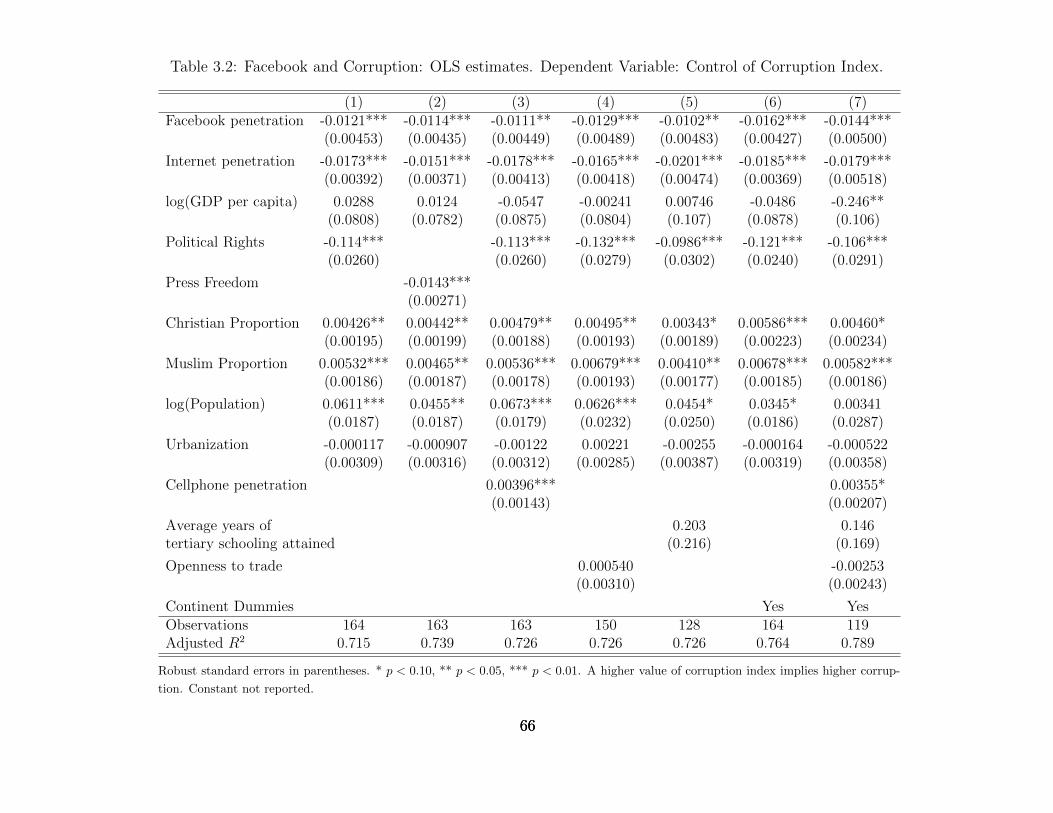
Table 3.2: Facebook and Corruption: OLS estimates. Dependent Variable: Control of Corruption Index.
(1) (2) (3) (4) (5) (6) (7)Facebook penetration -0.0121*** -0.0114*** -0.0111** -0.0129*** -0.0102** -0.0162*** -0.0144***
(0.00453) (0.00435) (0.00449) (0.00489) (0.00483) (0.00427) (0.00500)
Internet penetration -0.0173*** -0.0151*** -0.0178*** -0.0165*** -0.0201*** -0.0185*** -0.0179***(0.00392) (0.00371) (0.00413) (0.00418) (0.00474) (0.00369) (0.00518)
log(GDP per capita) 0.0288 0.0124 -0.0547 -0.00241 0.00746 -0.0486 -0.246**(0.0808) (0.0782) (0.0875) (0.0804) (0.107) (0.0878) (0.106)
Political Rights -0.114*** -0.113*** -0.132*** -0.0986*** -0.121*** -0.106***(0.0260) (0.0260) (0.0279) (0.0302) (0.0240) (0.0291)
Press Freedom -0.0143***(0.00271)
Christian Proportion 0.00426** 0.00442** 0.00479** 0.00495** 0.00343* 0.00586*** 0.00460*(0.00195) (0.00199) (0.00188) (0.00193) (0.00189) (0.00223) (0.00234)
Muslim Proportion 0.00532*** 0.00465** 0.00536*** 0.00679*** 0.00410** 0.00678*** 0.00582***(0.00186) (0.00187) (0.00178) (0.00193) (0.00177) (0.00185) (0.00186)
log(Population) 0.0611*** 0.0455** 0.0673*** 0.0626*** 0.0454* 0.0345* 0.00341(0.0187) (0.0187) (0.0179) (0.0232) (0.0250) (0.0186) (0.0287)
Urbanization -0.000117 -0.000907 -0.00122 0.00221 -0.00255 -0.000164 -0.000522(0.00309) (0.00316) (0.00312) (0.00285) (0.00387) (0.00319) (0.00358)
Cellphone penetration 0.00396*** 0.00355*(0.00143) (0.00207)
Average years of 0.203 0.146tertiary schooling attained (0.216) (0.169)
Openness to trade 0.000540 -0.00253(0.00310) (0.00243)
Continent Dummies Yes YesObservations 164 163 163 150 128 164 119Adjusted R2 0.715 0.739 0.726 0.726 0.726 0.764 0.789
Robust standard errors in parentheses. * p < 0.10, ** p < 0.05, *** p < 0.01. A higher value of corruption index implies higher corrup-
tion. Constant not reported.
666666
Next, we control for a number of variables in order to minimize the omitted variable bias.
First, we replace the political rights index with the press freedom index in the baseline spec-
ification and present the results in column 2. The reason for doing so is that the coefficient
of Facebook penetration may be capturing a part of the effect of press freedom on corrup-
tion when press freedom is omitted from the model. We use negative of the press freedom
index and therefore expect the coefficient of this variable to be negative. The coefficient of
Facebook penetration remains highly significant with the expected negative sign. In column
3, we control for cellphone penetration as they are also used as means of communication.
This does not seem to have much of an impact on the coefficient of internet penetration. It
has been shown that countries with higher human capital are less corrupt (Glaeser and Saks,
2006). Corruption is lower in more open countries (Ades and Di Tella, 1999) and greater in
countries with protectionist trade policies (Dutt, 2009). We find that our results are robust
to the inclusion of the average years of tertiary schooling attained (column 4) and openness
to trade (column 5). In column 6 we include continent dummies to rule out the possibility
that these results are driven by the omission of continent-fixed factors. Finally, column 7
controls for all the variables in the same specification along with continent dummies. The
coefficient of Facebook penetration is highly significant in each column with the expected
sign. Moreover, in all the specifications, the coefficient of internet penetration is highly
significant with the expected negative sign.
As argued earlier, many countries restrict freedom on the net making internet penetration
endogenous to the model and, therefore, the OLS estimates are likely to be biased. Hence,
in the next section, we present the two stage least squares (2SLS) estimates.
3.3.2 IV Results
Table 3.3 reports the results of the IV analysis using the 1500 communication technology as
an instrument for the internet penetration today. Column 1 in panel 1 shows that commu-
67
nication technology in 1500 AD is a significant predictor of internet penetration today. In
panel 2, we present the IV estimates. The coefficient of Facebook penetration appears with
the expected sign and is statistically significant at conventional levels. Next, we address
potential concerns regarding the validity of our instrument by controlling for a number of
historical as well as contemporary variables whose omission may lead to the violation of the
exclusion restriction.
First, there may be concerns that technology in 1500 AD might be correlated with in-
stitutions in 1500 AD, which might be correlated with institutions today. Since controlling
for modern institutions might lead to biased estimates, we control for the colonial status of
a country, which is exogenous, as a proxy for institutional quality. Acemoglu and Robin-
son (2001) argue that colonial status is a good proxy for institutions. Following previous
literature (Treisman, 2000 and Swamy et al., 2001), we include dummies for former British
colonies and countries that were never colonized (column 2).15 Column 3 controls for cultural
variables which are arguably exogenous to corruption (Treisman, 2000). In both the columns,
1500 communication technology remains a significant predictor of internet penetration today
and the coefficient of Facebook penetration is statistically significant.
There may still be a concern, however, that the countries that had better technology
in 1500 AD might have also had higher incomes. Those countries may have been able to
constrain corruption more effectively in the beginning which may persist over time. If this
is true, then we need to control for the income levels in 1500 AD. Though there are no data
available for income levels of countries in 1500 AD, following Acemoglu et al. (2002), we
control for the urbanization in 1500 AD as a proxy for economic prosperity of that period.16
There is another advantage of controlling for the urbanization rate in 1500 AD. It is possible
15 Our results are, however, robust to the inclusion of dummies for French colonies, Spanish and Portuguesecolonies, and colonies of countries other than Britain, France, Spain, and Portugal. We take the colonialstatus data from Treisman (2007).
16 Acemoglu et al. (2002) argue that urbanization and population density are good proxies for economicprosperity. However, they note that the association between population density and economic prosperity istheoretically weaker than that between urbanization and economic prosperity making the latter our preferredmeasure of economic prosperity in 1500 AD. We borrow this data from Acemoglu et al. (2002).
68
that there are some fixed factors which have an impact on technology adoption as well as
corruption. If these fixed factors are also correlated with income levels or urbanization, then
controlling for 1500 AD urbanization will partially address this issue as well. In addition, we
control for cultural factors by including the proportion of Christians and Muslims in the total
population as additional regressors. The estimates are then no longer biased by the omission
of the cultural factors that persist for centuries and have an impact on corruption as well
as technology adoption. Technology adoption in 1500 AD remains a significant predictor
of internet penetration today even after controlling for urbanization in 1500 AD (panel 1
column 4). In panel 2 (column 4), the coefficient of Facebook penetration is highly significant
with negative sign suggesting that Facebook penetration impacts corruption negatively.
Although these results are very convincing that Facebook penetration has a causal and
negative impact on corruption, owing to the cross-sectional nature of our analysis, in the
next three columns we control for a number of historical as well as contemporary variables
to check the robustness of our estimates.
First, we control for the years since neolithic revolution – years since humans moved from
a hunter-gatherer society to the agrarian society and began cultivating crops and domesti-
cating animals. Years since neolithic revolution has been recognized as an important factor
in determining the historical development (Olsson and Hibbs, 2005.) Hence, in column 5, we
control for the years since neolithic revolution along with urbanization and cultural controls.
One final concern could be that the general level of technology in 1500, which is likely to
be correlated with the technology adoption in communication in year 1500, may have an
effect on corruption via the use of technologies other than internet penetration. If this is
true, then our estimates may be biased upwards if the general level of technology adoption
is omitted from the model. In order to address this concern, we control for the general level
of technological adoption in 1500 (excluding communication technology) in column 6. Fi-
nally, in column 7, we control for a number of contemporaneous variables – GDP per capita,
69
population, urbanization, cellphone penetration, and openness to trade.17 The coefficient
of Facebook penetration appears with the expected sign across different specifications and
is statistically significant at conventional levels. Moreover, in all these specifications, the
coefficient of internet penetration is statistically significant and negative indicating that in-
ternet penetration has negative impact on corruption. These IV coefficients are somewhat
larger than the OLS estimates suggesting that OLS estimates are biased downwards because
of endogeneity. Furthermore, the F−statistic at the bottom of the table indicates that the
instrument is strong in each column.
The results presented in this section are robust and show that Facebook penetration
has a negative impact on corruption. Moreover, these effects are sizable – even with our
most conservative OLS (IV) estimates, a one-standard deviation increase in the Facebook
penetration leads to more than a one-fifth (one-fourth) of a standard deviation improvement
in the corruption index. Similarly, even with our most conservative estimate, in addition to
its impact on corruption through Facebook, a one-standard deviation increase in internet
penetration reduces corruption by about two-fifth of a standard deviation.
3.3.3 Robustness Checks
Sensitivity to the use of an alternative corruption index
Table 3.4 reports the results using the 2011 Corruption Perception Index published by
Transparency International.CPI takes values in the range of 1 to 10 where a higher number
represents lower corruption. We use the negative of this index in all our regressions and
therefore expect the coefficient Facebook penetration to be negative. We present results
for OLS, median, and robust regressions. In all the columns, the coefficient of Facebook
penetration is significant at conventional levels with expected sign.
17 Note that inclusion of contemporaneous variables is likely to induce bias in the estimated coefficients,however, the fact that the coefficients of both Facebook penetration and internet penetration are still highlysignificant and comparable to the coefficients reported in previous columns strengthens the confidence in theestimated coefficients.
70
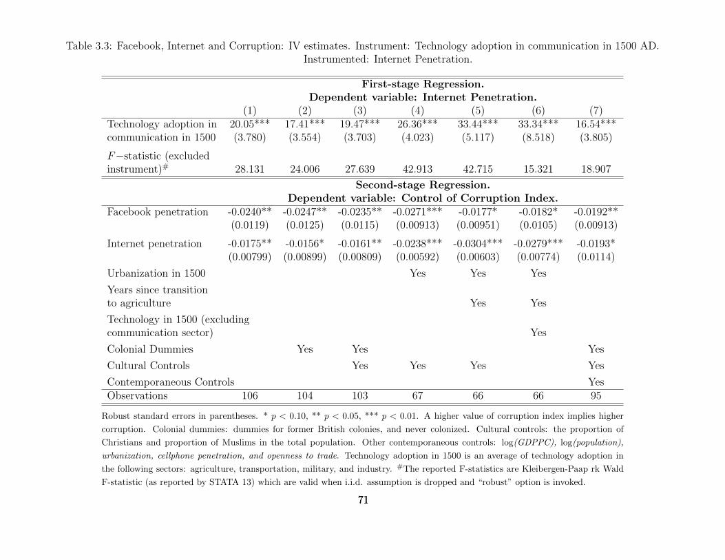
Table 3.3: Facebook, Internet and Corruption: IV estimates. Instrument: Technology adoption in communication in 1500 AD.Instrumented: Internet Penetration.
First-stage Regression.Dependent variable: Internet Penetration.
(1) (2) (3) (4) (5) (6) (7)Technology adoption in 20.05*** 17.41*** 19.47*** 26.36*** 33.44*** 33.34*** 16.54***communication in 1500 (3.780) (3.554) (3.703) (4.023) (5.117) (8.518) (3.805)
F−statistic (excludedinstrument)# 28.131 24.006 27.639 42.913 42.715 15.321 18.907
Second-stage Regression.Dependent variable: Control of Corruption Index.
Facebook penetration -0.0240** -0.0247** -0.0235** -0.0271*** -0.0177* -0.0182* -0.0192**(0.0119) (0.0125) (0.0115) (0.00913) (0.00951) (0.0105) (0.00913)
Internet penetration -0.0175** -0.0156* -0.0161** -0.0238*** -0.0304*** -0.0279*** -0.0193*(0.00799) (0.00899) (0.00809) (0.00592) (0.00603) (0.00774) (0.0114)
Urbanization in 1500 Yes Yes Yes
Years since transitionto agriculture Yes Yes
Technology in 1500 (excludingcommunication sector) Yes
Colonial Dummies Yes Yes Yes
Cultural Controls Yes Yes Yes Yes
Contemporaneous Controls YesObservations 106 104 103 67 66 66 95
Robust standard errors in parentheses. * p < 0.10, ** p < 0.05, *** p < 0.01. A higher value of corruption index implies higher
corruption. Colonial dummies: dummies for former British colonies, and never colonized. Cultural controls: the proportion of
Christians and proportion of Muslims in the total population. Other contemporaneous controls: log(GDPPC), log(population),
urbanization, cellphone penetration, and openness to trade. Technology adoption in 1500 is an average of technology adoption in
the following sectors: agriculture, transportation, military, and industry. #The reported F-statistics are Kleibergen-Paap rk Wald
F-statistic (as reported by STATA 13) which are valid when i.i.d. assumption is dropped and “robust” option is invoked.
717171
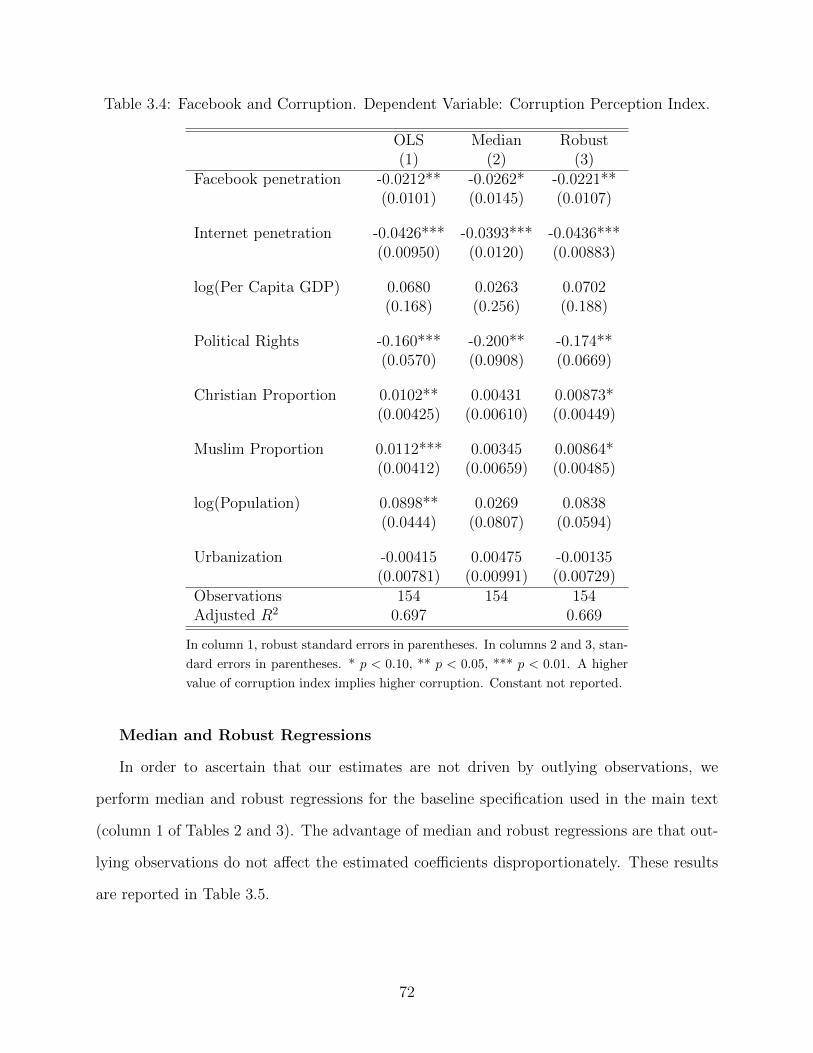
Table 3.4: Facebook and Corruption. Dependent Variable: Corruption Perception Index.
OLS Median Robust(1) (2) (3)
Facebook penetration -0.0212** -0.0262* -0.0221**(0.0101) (0.0145) (0.0107)
Internet penetration -0.0426*** -0.0393*** -0.0436***(0.00950) (0.0120) (0.00883)
log(Per Capita GDP) 0.0680 0.0263 0.0702(0.168) (0.256) (0.188)
Political Rights -0.160*** -0.200** -0.174**(0.0570) (0.0908) (0.0669)
Christian Proportion 0.0102** 0.00431 0.00873*(0.00425) (0.00610) (0.00449)
Muslim Proportion 0.0112*** 0.00345 0.00864*(0.00412) (0.00659) (0.00485)
log(Population) 0.0898** 0.0269 0.0838(0.0444) (0.0807) (0.0594)
Urbanization -0.00415 0.00475 -0.00135(0.00781) (0.00991) (0.00729)
Observations 154 154 154Adjusted R2 0.697 0.669
In column 1, robust standard errors in parentheses. In columns 2 and 3, stan-
dard errors in parentheses. * p < 0.10, ** p < 0.05, *** p < 0.01. A higher
value of corruption index implies higher corruption. Constant not reported.
Median and Robust Regressions
In order to ascertain that our estimates are not driven by outlying observations, we
perform median and robust regressions for the baseline specification used in the main text
(column 1 of Tables 2 and 3). The advantage of median and robust regressions are that out-
lying observations do not affect the estimated coefficients disproportionately. These results
are reported in Table 3.5.
72
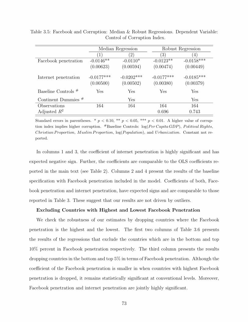
Table 3.5: Facebook and Corruption: Median & Robust Regressions. Dependent Variable:Control of Corruption Index.
Median Regression Robust Regression(1) (2) (3) (4)
Facebook penetration -0.0146** -0.0110* -0.0123** -0.0158***(0.00623) (0.00594) (0.00474) (0.00449)
Internet penetration -0.0177*** -0.0202*** -0.0177*** -0.0185***(0.00500) (0.00502) (0.00380) (0.00379)
Baseline Controls # Yes Yes Yes Yes
Continent Dummies # Yes YesObservations 164 164 164 164Adjusted R2 0.696 0.743
Standard errors in parentheses. * p < 0.10, ** p < 0.05, *** p < 0.01. A higher value of corrup-
tion index implies higher corruption. #Baseline Controls: log(Per CapitaGDP ), Political Rights,
ChristianProportion, MuslimProportion, log(Population), and Urbanization. Constant not re-
ported.
In columns 1 and 3, the coefficient of internet penetration is highly significant and has
expected negative sign. Further, the coefficients are comparable to the OLS coefficients re-
ported in the main text (see Table 2). Columns 2 and 4 present the results of the baseline
specification with Facebook penetration included in the model. Coefficients of both, Face-
book penetration and internet penetration, have expected signs and are comparable to those
reported in Table 3. These suggest that our results are not driven by outliers.
Excluding Countries with Highest and Lowest Facebook Penetration
We check the robustness of our estimates by dropping countries where the Facebook
penetration is the highest and the lowest. The first two columns of Table 3.6 presents
the results of the regressions that exclude the countries which are in the bottom and top
10% percent in Facebook penetration respectively. The third column presents the results
dropping countries in the bottom and top 5% in terms of Facebook penetration. Although the
coefficient of the Facebook penetration is smaller in when countries with highest Facebook
penetration is dropped, it remains statistically significant at conventional levels. Moreover,
Facebook penetration and internet penetration are jointly highly significant.
73
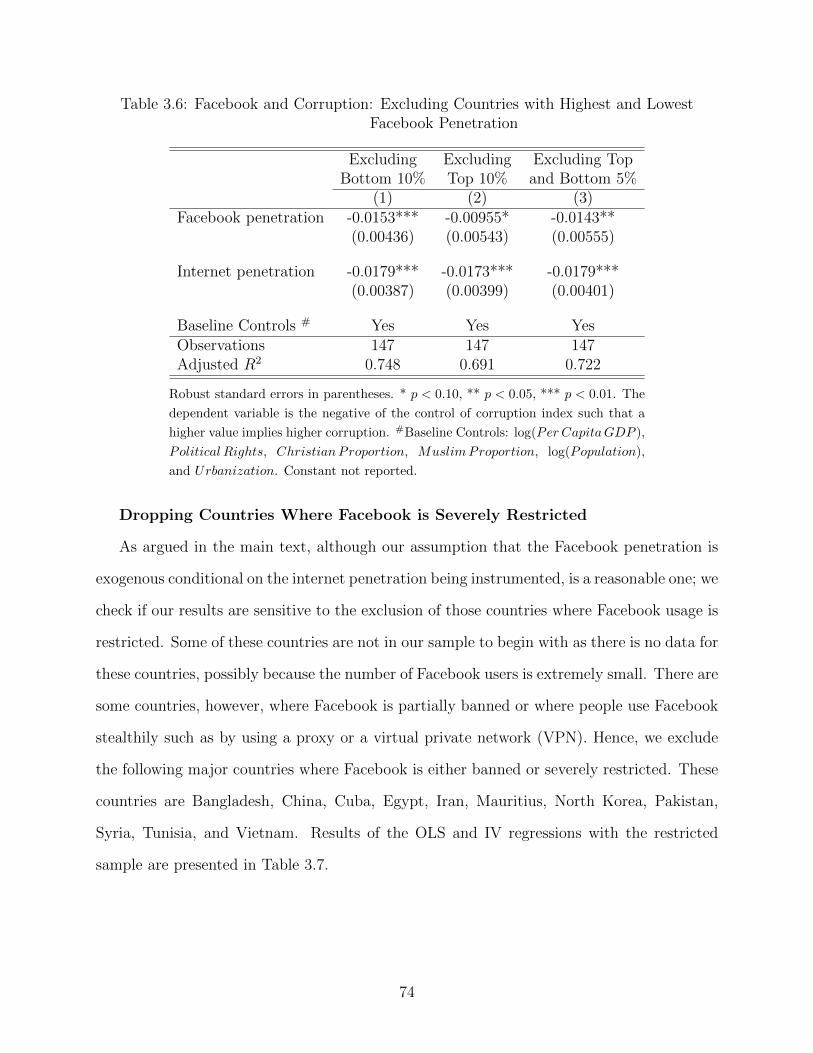
Table 3.6: Facebook and Corruption: Excluding Countries with Highest and LowestFacebook Penetration
Excluding Excluding Excluding TopBottom 10% Top 10% and Bottom 5%
(1) (2) (3)Facebook penetration -0.0153*** -0.00955* -0.0143**
(0.00436) (0.00543) (0.00555)
Internet penetration -0.0179*** -0.0173*** -0.0179***(0.00387) (0.00399) (0.00401)
Baseline Controls # Yes Yes YesObservations 147 147 147Adjusted R2 0.748 0.691 0.722
Robust standard errors in parentheses. * p < 0.10, ** p < 0.05, *** p < 0.01. The
dependent variable is the negative of the control of corruption index such that a
higher value implies higher corruption. #Baseline Controls: log(Per CapitaGDP ),
Political Rights, ChristianProportion, MuslimProportion, log(Population),
and Urbanization. Constant not reported.
Dropping Countries Where Facebook is Severely Restricted
As argued in the main text, although our assumption that the Facebook penetration is
exogenous conditional on the internet penetration being instrumented, is a reasonable one; we
check if our results are sensitive to the exclusion of those countries where Facebook usage is
restricted. Some of these countries are not in our sample to begin with as there is no data for
these countries, possibly because the number of Facebook users is extremely small. There are
some countries, however, where Facebook is partially banned or where people use Facebook
stealthily such as by using a proxy or a virtual private network (VPN). Hence, we exclude
the following major countries where Facebook is either banned or severely restricted. These
countries are Bangladesh, China, Cuba, Egypt, Iran, Mauritius, North Korea, Pakistan,
Syria, Tunisia, and Vietnam. Results of the OLS and IV regressions with the restricted
sample are presented in Table 3.7.
74
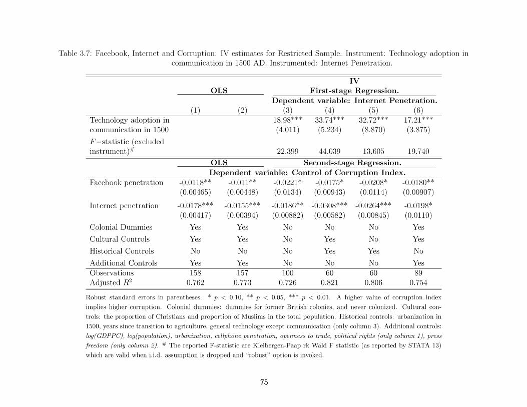
Table 3.7: Facebook, Internet and Corruption: IV estimates for Restricted Sample. Instrument: Technology adoption incommunication in 1500 AD. Instrumented: Internet Penetration.
IVOLS First-stage Regression.
Dependent variable: Internet Penetration.(1) (2) (3) (4) (5) (6)
Technology adoption in 18.98*** 33.74*** 32.72*** 17.21***communication in 1500 (4.011) (5.234) (8.870) (3.875)
F−statistic (excludedinstrument)# 22.399 44.039 13.605 19.740
OLS Second-stage Regression.Dependent variable: Control of Corruption Index.
Facebook penetration -0.0118** -0.011** -0.0221* -0.0175* -0.0208* -0.0180**(0.00465) (0.00448) (0.0134) (0.00943) (0.0114) (0.00907)
Internet penetration -0.0178*** -0.0155*** -0.0186** -0.0308*** -0.0264*** -0.0198*(0.00417) (0.00394) (0.00882) (0.00582) (0.00845) (0.0110)
Colonial Dummies Yes Yes No No No Yes
Cultural Controls Yes Yes No Yes No Yes
Historical Controls No No No Yes Yes No
Additional Controls Yes Yes No No No YesObservations 158 157 100 60 60 89Adjusted R2 0.762 0.773 0.726 0.821 0.806 0.754
Robust standard errors in parentheses. * p < 0.10, ** p < 0.05, *** p < 0.01. A higher value of corruption index
implies higher corruption. Colonial dummies: dummies for former British colonies, and never colonized. Cultural con-
trols: the proportion of Christians and proportion of Muslims in the total population. Historical controls: urbanization in
1500, years since transition to agriculture, general technology except communication (only column 3). Additional controls:
log(GDPPC), log(population), urbanization, cellphone penetration, openness to trade, political rights (only column 1), press
freedom (only column 2). # The reported F-statistic are Kleibergen-Paap rk Wald F statistic (as reported by STATA 13)
which are valid when i.i.d. assumption is dropped and “robust” option is invoked.
757575
In Table 3.7, the first two columns present the OLS estimates, and the last four columns
present IV estimates where internet penetration is instrumented with the technological adop-
tion in communication in 1500. As we can see, the relationship between the Facebook pen-
etration and corruption is highly statistically significant in each column. Moreover, these
coefficients are very stable across specifications and are comparable to those reported in the
main text in the analysis of the entire sample. These results provide an assurance that the
relationship between the Facebook penetration and corruption is not driven by the countries
that ban the use of Facebook.
3.4 Falsification test for the Facebook-corruption relationship
In order to further establish that the relationship between Facebook penetration and corrup-
tion is causal, we present a falsification test for the Facebook-corruption relationship in this
section. If our results are driven by omitted variables, then we should observe a significant
relationship between Facebook penetration and corruption even before Facebook came into
existence in 2003. In column 1 of Table 3.8, our dependent variable is the 1996 CCI. As
we can see, the coefficient of Facebook penetration is not significant conditional on internet
penetration and other control variables for the same year (see notes below the table). The
coefficient of Facebook penetration is small, has the expected sign and significant at the 10%
level when the dependent variable is the 2005 CCI in column 2. We believe that since Face-
book had only been launched in 2003, it was not yet popular enough to have a larger effect
by 2005. However, when the dependent variable is the 2011 CCI, the coefficient of Facebook
penetration is not only significant but also about 50 percent larger than the coefficient in
column 2. These estimates indicate that the results are not driven by some omitted variables
and Facebook penetration has a causal impact on corruption.
76
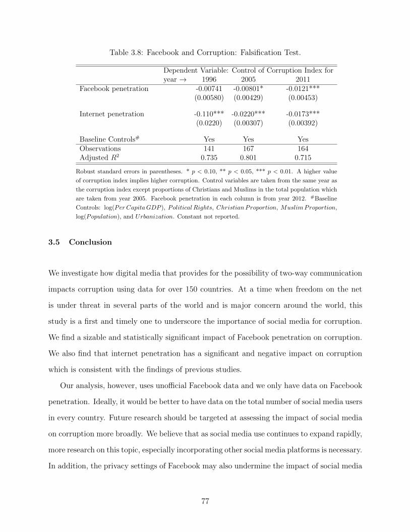
Table 3.8: Facebook and Corruption: Falsification Test.
Dependent Variable: Control of Corruption Index foryear → 1996 2005 2011
Facebook penetration -0.00741 -0.00801* -0.0121***(0.00580) (0.00429) (0.00453)
Internet penetration -0.110*** -0.0220*** -0.0173***(0.0220) (0.00307) (0.00392)
Baseline Controls# Yes Yes YesObservations 141 167 164Adjusted R2 0.735 0.801 0.715
Robust standard errors in parentheses. * p < 0.10, ** p < 0.05, *** p < 0.01. A higher value
of corruption index implies higher corruption. Control variables are taken from the same year as
the corruption index except proportions of Christians and Muslims in the total population which
are taken from year 2005. Facebook penetration in each column is from year 2012. #Baseline
Controls: log(Per CapitaGDP ), Political Rights, ChristianProportion, MuslimProportion,
log(Population), and Urbanization. Constant not reported.
3.5 Conclusion
We investigate how digital media that provides for the possibility of two-way communication
impacts corruption using data for over 150 countries. At a time when freedom on the net
is under threat in several parts of the world and is major concern around the world, this
study is a first and timely one to underscore the importance of social media for corruption.
We find a sizable and statistically significant impact of Facebook penetration on corruption.
We also find that internet penetration has a significant and negative impact on corruption
which is consistent with the findings of previous studies.
Our analysis, however, uses unofficial Facebook data and we only have data on Facebook
penetration. Ideally, it would be better to have data on the total number of social media users
in every country. Future research should be targeted at assessing the impact of social media
on corruption more broadly. We believe that as social media use continues to expand rapidly,
more research on this topic, especially incorporating other social media platforms is necessary.
In addition, the privacy settings of Facebook may also undermine the impact of social media
77
on corruption. Clearly, the degree of anonymity of users sharing their bribing experiences
may play a crucial role in the realization of the effect of social media on corruption. Future
research should also investigate this hypothesis.
78
Chapter 4. Effectiveness ofAsymmetric Liability Policy:A Theoretical Investigation
4.1 Introduction
The effectiveness of asymmetric liability policy on reducing bribe occurrences has recently
attracted considerable attention from researchers.1 A number of theoretical as well as exper-
imental papers investigate if asymmetric liability policy – policy that gives legal impunity
to bribe-givers, as opposed to symmetric liability policy under which the bribe-giver is also
considered to be an accomplice in the crime, has the potential to reduce bribery. The in-
tuition is simple – when the bribe-giver is considered to be an accomplice in the crime and
is, therefore, subject to legal sanctions he/she has little incentive to report bribery. On the
other hand, a bribe-giver is more likely to report having paid a bribe when she is awarded
legal immunity. In a world where a bribery is more likely to be discovered when it is reported
as opposed to when it is not reported, providing legal immunity to bribe-givers would result
in reduction in bribe demand by corrupt officials.
While the implementation of asymmetric liability policy may be relevant for all kinds
of bribes, its relevance for a special kind of bribes called harassment bribes or extortionary
bribes – where the bribe-giver is forced to pay a bribe for the services he/she is entitled to –
is considered to be relatively less debatable compared to collusive bribery – where a person
pays bribes in order to obtain undue favors.2
1 More recently, the asymmetric liability regime has been widely debated after Basu (2011) proposedlegal immunity to the bribe givers in India arguing that this policy will reduce bribery by increasing thebribe-reporting. He also proposes that bribe be refunded to the bribe giver, once bribery is established,to further incentivise bribe reporting. However, Basu’s policy has been criticized on several grounds (forexample, see Dreze (2011)). Note that in several countries such as China, Japan and Russia legal punishmentfor bribe-giver is milder than that for bribe-taker. On the other hand, countries such as Germany, UK, andUSA treat bribe-giver as well as bribe-taker equally culpable.
2 More specifically, the moral issues involved with the implementation of the asymmetric liability policy
79
The present chapter contributes to the literature studying the impact of asymmetric
liability policy on reducing bribery by investigating the effect of an alternative policy regime
which we call conditional legal immunity. The conditional legal immunity is a modification
of the asymmetric liability policy under which a bribe-giver is awarded legal immunity only
if she reports having paid a bribe, otherwise, she is considered as an accomplice in the crime
and is subject to legal consequences should the bribery be discovered just as under symmetric
liability policy. We find that conditional legal immunity is more effective in reducing bribery
in a theoretical setting. The paper most akin to the theoretical part of this chapter is
Dufwenberg and Spagnolo (2014) who also investigate the impact of an equivalent policy on
bribe occurrences and find that such a policy is more effective in reducing bribery than the
asymmetric liability policy. This chapter, however, is methodologically different than theirs,
and we derive conditions under which different policies will be successful.3
The rest of the chapter is organized as follows. The next section develops the theoretical
model and makes predictions for bribery under different policy regimes. Conclusions are
drawn in section 2.6.
4.2 The model set-up
The basics of the game are following. The citizen, C, is entitled to a license. The value of
the license to the citizen is v. The citizen, on the other hand, if is denied (or indefinitely
delayed) the license, has a payoff equal to 0. The official O can, however, indefinitely delay
has been an argument against the implementation of such policies. The critics argue that implementingasymmetric liability policy is likely to decrease the moral cost of bribery and may lead to the norm thatbribe paying is morally acceptable. This may lead to further increase in bribery. Also, providing legalimmunity may encourage citizens to offer bribes more often. Essentially, such policies will have more seriousnegative implications for collusive bribery. For instance, knowing that it would not be punished for payinga bribe should the bribery be discovered, a firm will have a larger incentive to pay bribes.
3 More specifically, in this chapter, whether or not the act of bribery will be discovered is a probabilisticevent. In contrast, in Dufwenberg and Spagnolo (2014) the official’s cost of providing services implicitlyincludes the probability with which a bribery can be discovered. By introducing the probabilities of discov-ering a bribery we are not only able evaluate which policies are likely to be effective in reducing bribery butwe can also derive conditions under which a policy is going to work.
80
issuing the license, and may exercise this power in order to extract bribes, b, from the citizen.
Once a bribe is demanded by the official, the citizen may choose to pay or reject. In the
event of paying the bribe, the citizen may further choose to report it or not.4 The cost of
reporting the bribe to the citizen is c.
The probability that a bribe incident will be discovered depends on whether or not it is
reported. If the bribe is reported the probability of bribe discovery is p and the corresponding
probability is p′ in case it is not reported where p > p′ > 0. Furthermore, also assume that
cost of issuing license to the official is zero.5
Further restrictions:
• It is optimal for the citizen to get a license even after paying a bribe, v − b ≥ 0
• A stronger restriction – the citizen is better off from having the license even after he
has to bribe and incur the cost of bribe reporting, i.e., v− b− c > 0. This assumption
is needed to ensure that it is always optimal for the citizen to pay the bribe rather
than go without the license.
4.3 The game
For simplicity, let’s assume that there is only one interaction between the official and the
citizen, and this is a common knowledge to both, the citizen and the official.6 The official
4 In order to simplify the analysis, we assume that the citizen does not report the demand of bribe if shechooses not to pay. It may be very difficult to prove that a bribe was demanded in case she does not paythe bribe.
5 This assumption is in contrast with the Dufwenberg and Spagnolo (2014) who allow for a non-zero costto the official of issuing the license. They assume that the cost of issuing the license is above zero if theofficial can spend this time in some other utility maximizing activity such as playing a computer game. Onthe other hand, the cost of issuing license is less than zero if the shirking is riskier and the probability ofgetting caught is substantial even though the bribe is not reported. We capture this possibility by addingthe ‘probability of getting caught’ in the model. Furthermore, we assume that even though the official canshirk from issuing the license, he has to be present in the office during regular hours, so the cost of issuinglicense to him is close to zero.
6 In many instances of harassment bribery, the assumption of single interaction may not be very far fromthe reality. For instance, a person facing the same clerk in the office of motor vehicles in countries like Indiais not very common as the driver’s license are issued for 20 years. The same thing may be true for passportoffices and other such services. Nevertheless, we relax this assumption later.
81
begins by either demanding a bribe (B) in the amount of b, or not demanding a bribe (¬B).
We assume that the official issues the license when he does not demand a bribe, and he
demands a bribe and gets one.7 Once the official demands a bribe, the citizen has three
available actions – don’t pay (¬P ), pay quietly (and not report) (¬R), and pay and report
(R). If the citizen refuses to pay, he is not granted the license. We further assume that
paying the bribe is always optimal for the citizen rather than go without the license given
the bribe has been demanded.8 Thus, the bribe-giver, once the bribe has been demanded,
chooses from two actions – to pay quietly, or to pay and report, given the values of other
parameters of the model. Also, the exchange of bribe and license takes place simultaneously,
and hence, there is not further action node for the official.
Under symmetric liability, as is currently the law, if a bribe is paid, both the parties
are considered to be partners in the crime. And, therefore, if a bribe incident is detected,
both are convicted and punished. The fine amount, however, may be different. Let the fine
imposed on official be fo, and on the citizen be fc.9
Under asymmetric liability where the bribe-giver is given legal immunity, if a bribe inci-
dent is detected the official is convicted while the citizen is let go. Basu, 2011 also proposes
that once the bribery is detected the bribe amount should be returned to the citizen. While
this proposal has been criticized on the grounds that it may be practically infeasible to re-
fund the bribe amount, we also consider this possibility. We, however, maintain that the
cost of reporting a bribe is still borne by the citizen. This is assumed based on the fact that
it may be even more difficult to determine the actual cost of reporting a bribe than the bribe
amount itself.
7 Following Dufwenberg and Spagnolo, 2014 we assume that bribe taking and license delivery takesplace simultaneously in contrast to Buccirossi and Spagnolo, 2006 where the two acts do not take placesimultaneously and an enforcement mechanism may be required. For most of the bribes falling underharassment category, usually the service is provided right away, and hence, the former is the obvious choice.
8 This assumption, though, can be relaxed, we maintain this assumption because this is very close toreality. The bribe amount in harassment bribery is seldom large enough relative to the value of services suchto make it worthwhile not to pay.
9 Basu, 2011 suggest doubling the fine for the official implying that fo = fc. However, this assumptionis not important for our analysis, nevertheless, while investigating the merits of Basu’s policy we double thefine of the official irrespective of the possibility that fc may or may not be same as fo.
82
We consider the following two possibilities under asymmetric liability regime:
A. Bribe not refunded (BNR): This is the simple asymmetric liability case in which
although the bribe giver is given the legal immunity, the bribe is not to be returned
even though the bribery is established in the court of law and bribe amount is detected.
B. Bribe Refunded (BR): The bribe-giver is given legal immunity and the bribe is
refunded, fine for the bribe taker is doubled (same as Basu’s proposal).
We consider some modifications in asymmetric liability policy and Basu’s policy. We call
this alternative policy conditional legal immunity. Under conditional legal immunity, the
bribe-giver is awarded legal impunity only if he/she reports having paid a bribe. If bribery
is discovered by other means, then the bribe-giver shall be treated as an accomplice in the
crime and symmetrical liability policy shall be applicable to her. We consider two variants
of conditional legal immunity:
A. Conditional legal immunity with no refund of bribe (CLI): If the bribe giver
reports having paid a bribe, the asymmetric liability policy will be applicable to her,
i.e. she will be given legal immunity. Otherwise, the bribe giver should be treated as
an accomplice in the crime as it is under the current law. The bribe amount is not
refunded. The bribe-taker is subject to twice the fine under symmetric liability.
B. Conditional legal immunity with bribe returned to the citizen (CLIB): If the
bribe-giver reports paying the bribe, not only is she given legal immunity but she is
also returned the bribe amount. She shall be treated an accomplice in the crime if the
bribery is discovered by other means.
Figure 4.1 represents the game. Payoffs associated with the symmetric liability is given
inside the parentheses (( )), and those inside the angle brackets (〈 〉) and curly brackets ({ })
are associated with BNR, and BR respectively. Payoffs inside the square brackets ([ ]) and
backslashes (\ \) are associated with CLI and CLIB respectively. The game can be solved
by the backward induction.
83

¬B
(0, v) O
B
¬P (0, 0)
C
¬R R
1-p' p' 1-p p
1. (b, v-b) (-fo, v-b-fc) (b, v-b-c) (-fo, v-b-c-fc)
2. ⟨b, v-b⟩ ⟨-fo, v-b⟩ ⟨b, v-b-c⟩ ⟨-fo, v-b-c⟩
3. {b, v-b} {-2fo, v} {b, v-b-c} {-2fo, v-c}
4. [b, v-b] [-fo, v-b-fc] [b, v-b-c] [-fo, v-b-c]
5. \b, v-b\ \-2fo, v-b-fc\ \b, v-b-c\ \-2fo, v-c\
Notes:
1. Symmetric liability: both the bribe-giver and the bribe-taker are culpable and subject to
legal sanctions.
2. BNR (Bribe not refunded): asymmetric liability – bribe-taker punished, bribe-giver
given legal impunity. Bribe not refunded.
3. BR (Bribe refunded): asymmetric liability – bribe-taker punished, bribe-giver given
legal impunity. Bribe refunded to the bribe-giver. Fine of bribe-taker doubled
4. CLI (conditional legal immunity): BNR applicable only if the bribery is reported by the
bribe-giver.
5. CLIB (Conditional legal immunity with bribe refunded): BR applicable only if the
bribery is reported by the bribe giver.
Figure 4.1: Single-interaction game: Symmetric vs. asymmetric liability
84
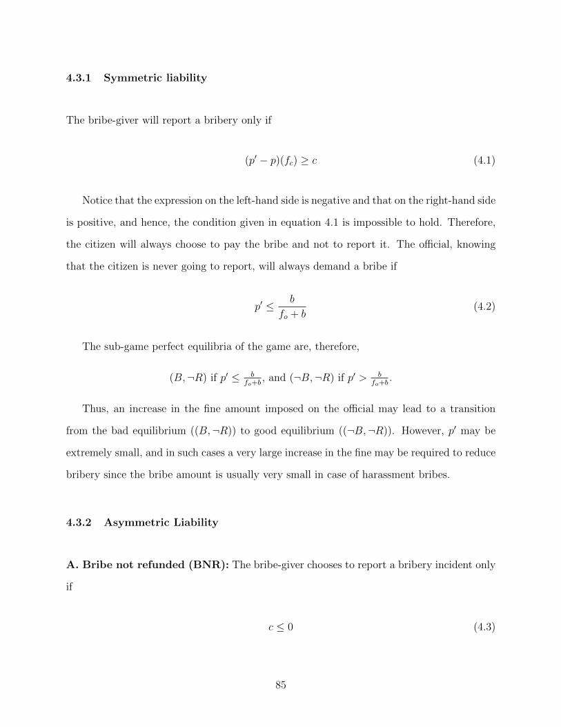
4.3.1 Symmetric liability
The bribe-giver will report a bribery only if
(p′ − p)(fc) ≥ c (4.1)
Notice that the expression on the left-hand side is negative and that on the right-hand side
is positive, and hence, the condition given in equation 4.1 is impossible to hold. Therefore,
the citizen will always choose to pay the bribe and not to report it. The official, knowing
that the citizen is never going to report, will always demand a bribe if
p′ ≤ b
fo + b(4.2)
The sub-game perfect equilibria of the game are, therefore,
(B,¬R) if p′ ≤ bfo+b
, and (¬B,¬R) if p′ > bfo+b
.
Thus, an increase in the fine amount imposed on the official may lead to a transition
from the bad equilibrium ((B,¬R)) to good equilibrium ((¬B,¬R)). However, p′ may be
extremely small, and in such cases a very large increase in the fine may be required to reduce
bribery since the bribe amount is usually very small in case of harassment bribes.
4.3.2 Asymmetric Liability
A. Bribe not refunded (BNR): The bribe-giver chooses to report a bribery incident only
if
c ≤ 0 (4.3)
85
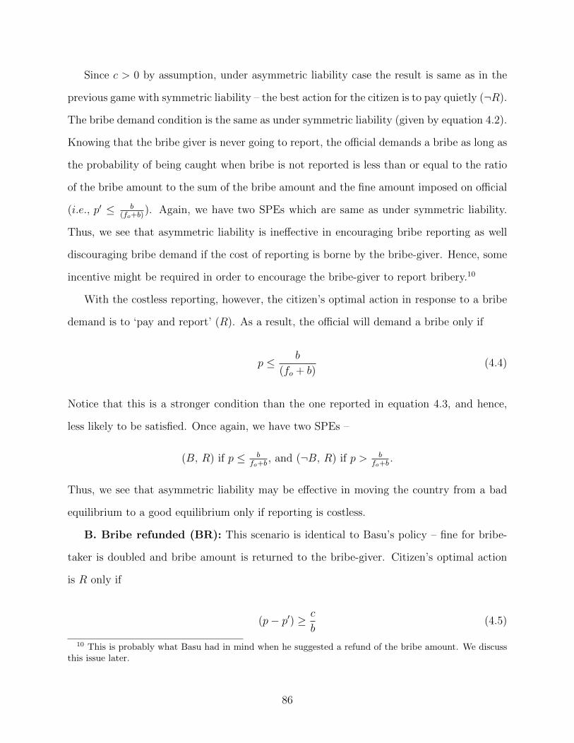
Since c > 0 by assumption, under asymmetric liability case the result is same as in the
previous game with symmetric liability – the best action for the citizen is to pay quietly (¬R).
The bribe demand condition is the same as under symmetric liability (given by equation 4.2).
Knowing that the bribe giver is never going to report, the official demands a bribe as long as
the probability of being caught when bribe is not reported is less than or equal to the ratio
of the bribe amount to the sum of the bribe amount and the fine amount imposed on official
(i.e., p′ ≤ b(fo+b)
). Again, we have two SPEs which are same as under symmetric liability.
Thus, we see that asymmetric liability is ineffective in encouraging bribe reporting as well
discouraging bribe demand if the cost of reporting is borne by the bribe-giver. Hence, some
incentive might be required in order to encourage the bribe-giver to report bribery.10
With the costless reporting, however, the citizen’s optimal action in response to a bribe
demand is to ‘pay and report’ (R). As a result, the official will demand a bribe only if
p ≤ b
(fo + b)(4.4)
Notice that this is a stronger condition than the one reported in equation 4.3, and hence,
less likely to be satisfied. Once again, we have two SPEs –
(B, R) if p ≤ bfo+b
, and (¬B, R) if p > bfo+b
.
Thus, we see that asymmetric liability may be effective in moving the country from a bad
equilibrium to a good equilibrium only if reporting is costless.
B. Bribe refunded (BR): This scenario is identical to Basu’s policy – fine for bribe-
taker is doubled and bribe amount is returned to the bribe-giver. Citizen’s optimal action
is R only if
(p− p′) ≥ c
b(4.5)
10 This is probably what Basu had in mind when he suggested a refund of the bribe amount. We discussthis issue later.
86

The above condition implies that the citizen is more likely to report the bribe if
1. the bribe amount, b, is very high.
2. the difference between the probability of conviction under reporting and that under
not reporting (p−p′), is high implying that the probability of detection is significantly
higher when bribery is reported.
3. cost of reporting, c, is low.
The citizen now chooses to ‘pay and report’ as long as the difference between p and p′
is greater than the ratio of cost of reporting and bribe amount. This condition implies that
BR (or Basu’s policy) would be effective in encouraging bribe reporting only if the cost of
reporting a bribe is less than the bribe amount itself. This is a less stringent requirement
than the cost of reporting being zero as in asymmetric liability case where the bribe is not
refunded. Clearly, under BR, the likelihood of bribe reporting is higher than it is under
the asymmetric liability regime. However, BR does not necessarily guarantee a higher rate
of reporting and will be ineffective if corruption is so rampant in a country that reporting
increases the likelihood of a bribe detection only marginally, and the cost of reporting is high
relative to bribe amount.11
BR is also more likely to reduce bribe demand even if it is not successful in inducing
bribe reporting. There are two possible scenarios:
i. (p−p′) < cb: the bribe-giver does not report having paid a bribe. Therefore, the official
is likely to demand a bribe only if
p′ ≤ b
2fo + b(4.6)
11 This concern is of particular importance for countries like India where the judicial process is highlyinefficient and very lengthy, often taking years. Thus, it is quite possible that despite its obvious merits, BPmight be ineffective in inducing bribe reporting in countries like India. BP may, therefore, be more effectivein deterring bribery in countries where the cost of reporting is not exorbitantly high.
87
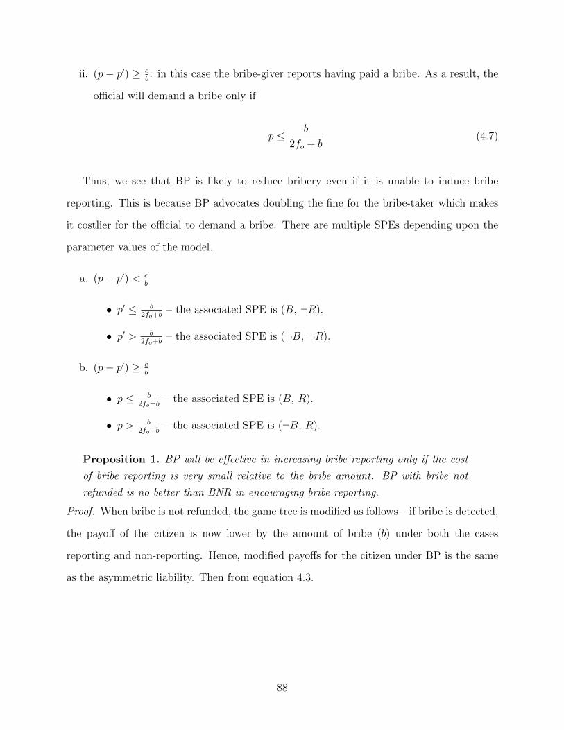
ii. (p− p′) ≥ cb: in this case the bribe-giver reports having paid a bribe. As a result, the
official will demand a bribe only if
p ≤ b
2fo + b(4.7)
Thus, we see that BP is likely to reduce bribery even if it is unable to induce bribe
reporting. This is because BP advocates doubling the fine for the bribe-taker which makes
it costlier for the official to demand a bribe. There are multiple SPEs depending upon the
parameter values of the model.
a. (p− p′) < cb
• p′ ≤ b2fo+b
– the associated SPE is (B, ¬R).
• p′ > b2fo+b
– the associated SPE is (¬B, ¬R).
b. (p− p′) ≥ cb
• p ≤ b2fo+b
– the associated SPE is (B, R).
• p > b2fo+b
– the associated SPE is (¬B, R).
Proposition 1. BP will be effective in increasing bribe reporting only if the cost
of bribe reporting is very small relative to the bribe amount. BP with bribe not
refunded is no better than BNR in encouraging bribe reporting.
Proof. When bribe is not refunded, the game tree is modified as follows – if bribe is detected,
the payoff of the citizen is now lower by the amount of bribe (b) under both the cases
reporting and non-reporting. Hence, modified payoffs for the citizen under BP is the same
as the asymmetric liability. Then from equation 4.3.
88
4.3.3 Conditional Legal Immunity
A. Conditional legal immunity with no refund of bribe (CLI): Following the crit-
icisms that it might be difficult to determine the actual bribe amount, we begin with the
case in which the bribe amount is not refunded. In this case, the bribe-giver chooses to ‘pay
and report’ if
p′ ≥ c
fc(4.8)
The above condition implies that the citizen is more likely to report the bribery if
1. the fine imposed on the bribe-giver, if she does not report and bribery is detected, is
very high,
2. the probability of conviction when bribery is not reported, p′, is high, and
3. cost of reporting, c, is low.
The bribe demand condition for the official is same as it is in symmetric liability case
and is given by equation 4.2. The SPEs associated with the CLI are given below:
a. p′ ≥ cfc
• p ≤ bfo+b
– the associated SPE is (B, R).
• p > bfo+b
– the associated SPE is (¬B, R).
b. p′ < cfc
• p′ ≤ bfo+b
– the associated SPE is (B, ¬R).
• p′ > bfo+b
– the associated SPE is (¬B, ¬R).
The above condition implies that a bribe-giver is more likely to report the bribery under
conditional legal immunity than under NBR.
89
B. Conditional legal immunity with bribe refunded (CLIB): What happens if
the bribe is refunded to the citizen and the official is fined twice the amount that is to be
paid under symmetric liability as suggested by Basu (2011)? The bribe-giver will report
having paid a bribe only if
bp+ p′fc ≥ c (4.9)
1. the fine imposed on the bribe-giver, if she does not report and bribery is detected, is
very high
2. the probability of conviction, when the bribe-giver reports the bribery and does not
report the bribery, p and p′, is high, and
3. cost of reporting, c, is low.
The official’s optimal action is the same as under BR depending on whether or not the
bribe-giver reports the bribery. If bp+ p′fc ≥ c, then official’s optimal action is given by 4.6,
and when bp+ p′fc < c, then official’s optimal action is given by 4.7.
The SPEs associated with the CLIB are given below:
a. bp+ p′fc ≥ c
• p ≤ b2fo+b
– the associated SPE is (B, R).
• p > b2fo+b
– the associated SPE is (¬B, R).
b. bp+ p′fc < c
• p′ ≤ b2fo+b
– the associated SPE is (B, ¬R).
• p′ > b2fo+b
– the associated SPE is (¬B, ¬R).
The citizen, therefore, chooses to report if the probability that the bribery will be de-
tected, even when she does not report it, is greater than the ratio of the cost of reporting
and the sum of payoff from having the license and the fine imposed on the bribe-giver.
90
The following propositions summarize the findings of this section.
Proposition 2. Conditional legal immunity with bribe refunded (CLIB) is more
likely to increase the bribe reporting than BR (or BP), and hence, more likely to
deter bribes than BR (or BP).
Proof. Comparing equations 4.5 and 4.9. CLI more effective if
bp+ p′fc > bp− bp′
=⇒ p′fc > −bp′
Since LHS is positive and RHS is negative, the above condition always holds. And hence,
CLI is more likely to increase the bribe reporting than BP when bribe is refunded under CLI
just like in BP.
Proposition 3. If the bribe amount is not refunded, then CLI performs better
than BR (or BP) in inducing bribe reporting only if the ratio of the difference
between the two probabilities of bribe detection (under reporting and non-reporting,
i.e., p − p′) and the probability of bribe detection when it is not reported by the
bribe-giver, is less than the ratio of fine imposed on the bribe-giver to the bribe
amount.
Proof. Comparing equation 4.5 and 4.8. CLI works better in inducing bribe reporting by
the bribe-giver than BP if
p′fc > b(p− p′)
=⇒ p− p′
p′<fcb
The above propositions suggests that in order to encourage the reporting under condi-
tional legal immunity, the probability of detection when bribery is not reported must be
91

significantly greater than zero, and the fine imposed on the citizen must be significantly
greater than the bribe amount.
4.4 Conclusion
Harassment bribes are widely prevalent in many developing countries of the world. These
bribes are often small in the amount relative to the benefit from the corresponding services.
However, these bribes cause great inconvenience to the lives of ordinary and poor people.
The most affected section of the society are the poorest and the prevalence of bribery denies
them access to the basic health and education facilities because the poor are unable to pay
bribes in many instances. Since in such types of bribes, the borrowers do not receive any
undue favors and are forced to pay the bribe even for the services they are entitle to, these
bribes are known as harassment or extortionary bribes. In view of this fact, some researchers
have proposed the idea that in case of this special class of bribes, the bribe givers should
be given legal immunity. The proponents of such policies argue that an asymmetric liability
policy would induce bribe givers to report bribe incidences leading to fall in the bribery.
This chapter explores the possibility that an asymmetric liability policy can reduce bribe
occurrences by encouraging the reporting of bribes. The theoretical findings indicate that an
asymmetric liability policy may not be enough in reducing bribery. A high cost of reporting
and establishing the bribery undermines the effectiveness of an asymmetric liability policy
and, hence, it needs to be complemented with other incentive mechanisms. A modification
in the asymmetric liability policy is suggested and is shown to be more effective in curbing
bribery.
92
Chapter 5. Conclusions
This dissertation investigates three important issues related to corruption in three dif-
ferent essays. The first two essays of the dissertation are empirical, and the third essay
develops a theoretical model. Some of the issues taken up in this dissertation had earlier
been investigated by previous studies but needed further investigation since the findings were
ambiguous. For instance, the causality between gender and corruption was not established
by the previous studies and the second chapter of this dissertation addresses the concerns for
causality in this literature. Some other issues have been investigated for the first time in this
thesis. For example, Chapter 3 of this dissertation is the first quantitatively comprehensive
study that investigates whether the social media can have a negative impact on corruption.
Finally, Chapter 4 adds to the existing literature on the legal system and bribery by inves-
tigating some of the contemporary issues and hypotheses by building upon previous studies
and extending the previous analysis. The main findings of this thesis are summarized below
with the possible extensions and the policy suggestions.
It is women’s presence only in politics that matters for corruption. Women’s presence in
other positions such as decision-making positions, clerical positions, and the labor force does
not have any impact on corruption. These findings suggest that women policymakers are
affecting corruption since they tend to choose different policies than men. The future work
on this topic should explore the channels through which women, as policy makers, are able
to affect corruption more extensively. Identifying the policies that reduce corruption will be
an important step towards understanding the causal link between women’s representation
in politics and corruption. Although the thesis provides suggestive evidence that gender
differences in social status do not seem to be driving the association between gender and
corruption, more research on this topic is required and may provide further insights on the
interaction between gender and corruption.
93
Facebook penetration and internet penetration are negatively related to corruption. So-
cial media and the internet, therefore, have a potential to fight against corruption through
an increase in transparency, facilitating the communication, and curtailing the ability of
authoritarian governments to control the transmission of information. As a result, acts of
corruption and bribery become more costly to commit as there are greater chances that
the act will be discovered. The future research should employ the social media usage more
broadly and investigate the impact of social media platforms, such as Twitter, Google Plus,
and YouTube, along with Facebook, on corruption. The role of blogs, technological advance-
ments that allow for greater anonymity in using websites, and the privacy settings of social
media platforms in affecting corruption should also be explored.
Finally, awarding legal immunity to the bribe givers may not be sufficient to reduce
bribery in the case of harassment bribes. Therefore, an asymmetric liability policy may fail
to deliver desired outcomes, especially in countries where corruption is so rampant that the
cost of bribe reporting is extremely high. A modification in the asymmetric liability policy,
therefore, is required that further incentivizes the bribe giver to report the bribe incident.
One such modification could be a situation where the bribe giver is given legal immunity
only when he/she reports the bribery.
Corruption is an issue whose solution requires concerted efforts from various sections of
the public and the policymakers. In order to successfully fight corruption, multiple actions
need to be taken in different areas such as empowering the disadvantaged sections of the
society, increasing the accessibility of technology, improving the institutional quality and
the effectiveness of the legal system, creating a culture of transparency, lessen hierarchy,
instilling moral values, restructuring the incentive mechanisms for public employees, and
creating awareness. This dissertation identifies three instruments that can be used to fight
corruption.
Following are the policy implications that emerge from this dissertation. Women’s em-
powerment in politics and government should be encouraged. Policies that promote women’s
94
political empowerment have positive externalities as, apart from achieving the much-needed
gender equality, they are also likely to impact corruption negatively. Infrastructural facilities
that make internet accessible to all should be provided. Freedom and transparency on the net
including social media should be promoted. The scope of e-governance should be expanded.
For the class of extortionary bribes, the implementation of an asymmetric liability policy
that is milder on the bribe-giver and harsher on the bribe-taker, should be contemplated
and debated. There is also a need for further incentivization in order to make bribe-givers
report bribery, either through a punishment mechanism or through making bribe-reporting
easier or reducing the probability that the bribe-taker might retaliate. Similar policies must
be explored for the collusive bribery.
95
References
1. Acemoglu, D. and J A Robinson. 2000. “Why did the West extend the franchise?Democracy, inequality, and growth in historical perspective.” Quarterly Journal ofEconomics 115.4, 1167–1199.
2. — . 2001. “The Colonial Origins of Comparative Development: An Empirical Inves-tigation.” American Economic Review 91.5, 1369–1401.
3. Acemoglu, Daron, Simon Johnson, and J A Robinson. 2002. “Reversal of fortune:Geography and institutions in the making of the modern world income distribution.”Quarterly Journal of Economics, 1231–1294.
4. Acemoglu, Daron, Simon Johnson, James A Robinson, and Pierre Yared. 2008. “Incomeand Democracy”. American Economic Review 98.3, 808–842.
5. Ades, Alberto and Rafael Di Tella. 1999. “Rents, competition, and corruption”. Amer-ican Economic Review, 982–993.
6. Agerberg, Mattias. 2014. “Gender Differences in the EQI Data”. QoG Working PaperSeries 2014.14, 14.
7. Alatas, Vivi, Lisa Cameron, Ananish Chaudhuri, Nisvan Erkal, and Lata Gangadha-ran. 2009. “Gender, culture, and corruption: Insights from an experimental analysis”.Southern Economic Journal 75.3, 663–680.
8. Alesina, Alberto, Paola Giuliano, and Nathan Nunn. 2013. “On the Origins of GenderRoles: Women and the Plough”. Quarterly Journal of Economics 128.2, 469–530.
9. Andersen, Thomas Barnebeck, Jeanet Bentzen, Carl-Johan Dalgaard, and Pablo Se-laya. 2011. “Does the Internet Reduce Corruption? Evidence from US States and acrossCountries”. World Bank Economic Review 25.3, 387–417.
10. Anderson, Theodore W and Herman Rubin. 1949. “Estimation of the parameters of asingle equation in a complete system of stochastic equations”. Annals of MathematicalStatistics, 46–63.
11. Barro, Robert J and Jong Wha Lee. 2013. “A new data set of educational attainmentin the world, 1950–2010”. Journal of Development Economics 104, 184–198.
12. Basu, Kaushik. 2011. “Why, for a Class of Bribes, the Act of Giving a Bribe should beTreated as Legal”.
13. Branisa, Boris, Stephan Klasen, and Maria Ziegler. 2009. “Background Paper: TheConstruction of the Social Institutions and Gender Index (SIGI)”.
96
14. Branisa, Boris, Stephan Klasen, and Maria Ziegler. 2013. “Gender inequality in socialinstitutions and gendered development outcomes”. World Development 45, 252–268.
15. Brunetti, Aymo and Beatrice Weder. 2003. “A free press is bad news for corruption”.Journal of Public Economics 87.7, 1801–1824.
16. Buccirossi, Paolo and Giancarlo Spagnolo. 2006. “Leniency policies and illegal trans-actions”. Journal of Public Economics 90.6, 1281–1297.
17. Campante, Filipe R, Davin Chor, and QUOC-ANH DO. 2009. “Instability and theIncentives for Corruption”. Economics & Politics 21.1, 42–92.
18. Cha, Jiyoung. 2010. “Factors affecting the frequency and amount of social networkingsite use: Motivations, perceptions, and privacy concerns”. First Monday 15.12.
19. Charron, Nicholas, Victor Lapuente, Bo Rothstein, A Varraish, and M Hernandez.2011. “Measuring quality of government and sub-national variation”. Report for theEU Commission of Regional Development, European Commission. Directorate-GeneralRegional Policy.
20. Chattopadhyay, Raghabendra and Esther Duflo. 2004. “Women as policy makers: Ev-idence from a randomized policy experiment in India”. Econometrica 72.5, 1409–1443.
21. Chen, M Keith. 2013. “The effect of language on economic behavior: Evidence fromsavings rates, health behaviors, and retirement assets”. American Economic Review103.2, 690–731.
22. Christiansen, Morten H and Simon Kirby. 2003. Language Evolution. Oxford UniversityPress.
23. Clots-Figueras, Irma. 2011. “Women in politics: Evidence from the Indian States”.Journal of Public Economics 95.7, 664–690.
24. Collier, Paul and Anke Hoeffler. 2005. “The Economic Cost of Corruption in Infras-tructure.” Global Corruption Report, Transparency International.
25. Comin, Diego, William Easterly, and Erick Gong. 2010. “Was the Wealth of NationsDetermined in 1000 BC?” American Economic Journal: Macroeconomics, 65–97.
26. Comin, Diego A and Bart Hobijn. 2009. The CHAT dataset. Tech. rep. National Bureauof Economic Research.
27. Dalacoura, Katerina. 2012. “The 2011 uprisings in the Arab Middle East: politicalchange and geopolitical implications”. International Affairs 88.1, 63–79.
28. Diamond, Larry. 2010. “Liberation technology”. Journal of Democracy 21.3, 69–83.
29. DiRienzo, Cassandra E, Jayoti Das, Kathryn T Cort, and John Burbridge. 2007. “Cor-ruption and the role of information”. Journal of International Business Studies 38.2,320–332.
97
30. Dollar, David, Raymond Fisman, and Roberta Gatti. 2001. “Are women really thefairer sex? Corruption and women in government”. Journal of Economic Behavior &Organization 46.4, 423–429.
31. Dreze, Jean. 2011. “The bribing game”. Indian Express April 23.
32. Dufwenberg, Martin and Giancarlo Spagnolo. 2014. “Legalizing Bribe Giving”. CEPRDiscussion Paper No. DP9236.
33. Dutt, Pushan. 2009. “Trade protection and bureaucratic corruption: an empirical in-vestigation”. Canadian Journal of Economics/Revue canadienne d’economique 42.1,155–183.
34. Eckel, Catherine C and Philip J Grossman. 1998. “Are women less selfish than men?:Evidence from dictator experiments”. Economic Journal 108.448, 726–735.
35. Elbahnasawy, Nasr G. 2014. “E-government, internet adoption, and corruption: Anempirical investigation”. World Development 57, 114–126.
36. Elbahnasawy, Nasr G and Charles F Revier. 2012. “The Determinants of Corruption:Cross-Country-Panel-Data Analysis”. Developing Economies 50.4, 311–333.
37. Esarey, Justin and Gina Chirillo. 2013. “Fairer Sex or Purity Myth? Corruption, Gen-der, and Institutional Context”. Politics & Gender 9.04, 361–389.
38. Finlay, Keith and Leandro M Magnusson. 2009. “Implementing weak-instrument robusttests for a general class of instrumental-variables models”. Stata Journal 9.3, 398.
39. Fisman, Raymond and Edward Miguel. 2007. “Corruption, norms, and legal enforce-ment: Evidence from diplomatic parking tickets”. Journal of Political Economy 115.6,1020–1048.
40. Frank, Bjorn, Johann Graf Lambsdorff, and Frederic Boehm. 2011. “Gender and cor-ruption: Lessons from laboratory corruption experiments”. European Journal of De-velopment Research 23.1, 59–71.
41. Freedom House. 2009. “Freedom on the net: A global assessment of internet and digitalmedia”.
42. Gay, Victor, Estefania Santacreu-Vasut, and Amir Shoham. 2014. “Language and Gen-der Economics”. Working Paper.
43. Glaeser, Edward L and Raven E Saks. 2006. “Corruption in America”. Journal ofPublic Economics 90.6, 1053–1072.
44. Goel, Rajeev K, Michael A Nelson, and Michael A Naretta. 2012. “The internet asan indicator of corruption awareness”. European Journal of Political Economy 28.1,64–75.
45. Goetz, Anne Marie. 2007. “Political Cleaners: Women as the new anti-corruptionforce?” Development and Change 38.1, 87–105.
98
46. Greene, William H. 2012. “Econometric Analysis”.
47. Gupta, Sanjeev, Hamid Davoodi, and Rosa Alonso-Terme. 2002. “Does corruptionaffect income inequality and poverty?” Economics of Governance 3.1, 23–45.
48. Hansen, Casper Worm, Peter S Jensen, and Christian Skovsgaard. 2012. “ModernGender Roles and Agricultural History: The Neolithic Inheritance”. Available at SSRN2170945.
49. Howard, Philip N and Muzammil M Hussain. 2011. “The role of digital media”. Journalof Democracy 22.3, 35–48.
50. Islam, Roumeen. 2006. “Does more transparency go along with better governance?”Economics & Politics 18.2, 121–167.
51. Jha, Chandan Kumar. 2014. “Can social media and internet help reduce corruption?”Available at http:// www.ideasforindia.in/ article.aspx?article id=353 .
52. Kangle, Ramakant Prabha. 2000. The Kautiliya Arthasastra. Motilal Banarsidass Pub-lication.
53. Kaufmann, Daniel, Aart Kraay, and Massimo Mastruzzi. 2011. “The worldwide gov-ernance indicators: methodology and analytical issues”. Hague Journal on the Rule ofLaw 3.02, 220–246.
54. Kedzie, Christopher. 1997. “Communication and democracy: Coincident revolutionsand the emergent dictators”.
55. Kleibergen, Frank. 2002. “Pivotal statistics for testing structural parameters in instru-mental variables regression”. Econometrica 70.5, 1781–1803.
56. Kudva, Neema. 2003. “Engineering elections: The experiences of women in PanchayatiRaj in Karnataka, India”. International Journal of Politics, Culture, and Society 16.3,445–463.
57. La Porta, Rafael, Florencio Lopez-de Silanes, Andrei Shleifer, and Robert W Vishny.1997. “Trust in Large Organizations”. American Economic Review 87.2, 333–338.
58. — . 1998. “Law and Finance”. Journal of Political Economy 106.6, 1113–1155.
59. Lambsdorff, Johann Graf. 2007. The institutional economics of corruption and reform:theory, evidence and policy. Cambridge University Press.
60. — . 2008. The methodology of the corruption perceptions index 2008. TransparencyInternational and University of Passau. Available at http://www.icgg.org/downloads/Methodology 2008.pdf (accessed May 14, 2015).
61. Lederman, Daniel, Norman V Loayza, and Rodrigo R Soares. 2005. “Accountabilityand corruption: Political institutions matter”. Economics & Politics 17.1, 1–35.
99
62. Mauro, Paolo. 1995. “Corruption and growth”. Quarterly Journal of Economics 110.3,681–712.
63. Moreira, Marcelo J. 2003. “A conditional likelihood ratio test for structural models”.Econometrica 71.4, 1027–1048.
64. Murray, Michael P. 2006a. “Avoiding invalid instruments and coping with weak instru-ments”. Journal of Economic Perspectives 20.4, 111–132.
65. — . 2006b. “The bad, the weak, and the ugly: Avoiding the pitfalls of instrumentalvariables estimation”. Available at SSRN 843185.
66. Nierhoff, Maximilian H. 2013. “Facebook Country Statistics May 2013 – Rough Esti-mates Or Something?” Retrieved from http://www.quintly.com/blog/2013/05/facebook-country-statistics-may-2013/.
67. North, Douglass C, William Summerhill, and Barry R Weingast. 2000. “Order, disor-der, and economic change: Latin America vs. North America”. Governing for Prosperity19.
68. Olsson, Ola and Douglas A Hibbs. 2005. “Biogeography and long-run economic devel-opment”. European Economic Review 49.4, 909–938.
69. Rehavi, M Marit. 2007. “Sex and politics: Do female legislators affect state spending?”Unpublished manuscript, University of Michigan.
70. Reynolds, Andrew. 1999. “Women in the legislatures and executives of the world:Knocking at the highest glass ceiling”. World Politics 51.04, 547–572.
71. Rule, Wilma and Joseph Francis Zimmerman. 1994. Electoral systems in comparativeperspective: Their impact on women and minorities. 338. Greenwood Publishing Group.
72. Sago, Brad. 2013. “Factors Influencing Social Media Adoption and Frequency of Use:An Examination of Facebook, Twitter, Pinterest and Google+.” International Journalof Business & Commerce 3.1.
73. Saleh, Nivien. 2012. “Egypts digital activism and the Dictators Dilemma: An evalua-tion”. Telecommunications Policy 36.6, 476–483.
74. Sullivan, Michael J. 1991. Measuring global values: The ranking of 162 countries. Green-wood Press New York.
75. Sundstrom, Aksel. 2013. “Womens Local Political Representation Within 30 EuropeanCountries”. QoG Working Paper Series 2013.18, 18.
76. Sundstrom, Aksel and Lena Wangnerud. 2014. “Corruption as an obstacle to womenspolitical representation: Evidence from local councils in 18 European countries”. PartyPolitics.
77. Sung, Hung-En. 2003. “Fairer sex or fairer system? Gender and corruption revisited”.Social Forces 82.2, 703–723.
100
78. Swamy, Anand, Stephen Knack, Young Lee, and Omar Azfar. 2001. “Gender and Cor-ruption”. Journal of Development Economics 64.1, 25.
79. Taylor-Robinson, Michelle M and Roseanna Michelle Heath. 2003. “Do women legis-lators have different policy priorities than their male colleagues? A critical case test”.Women & Politics 24.4, 77–101.
80. Thomas, Sue. 1991. “The impact of women on state legislative policies”. Journal ofPolitics 53.04, 958–976.
81. Treisman, Daniel. 2000. “The causes of corruption: a cross-national study”. Journal ofPublic Economics 76.3, 399–457.
82. — . 2007. “What have we learned about the causes of corruption from ten years ofcross-national empirical research?” Annual Review of Polititical Science 10, 211–244.
83. United Nations. 2012. “The Millennium Development Goals Report 2012”.
84. Wagner, Ben. 2012. “Push-button-autocracy in Tunisia: Analysing the role of Internetinfrastructure, institutions and international markets in creating a Tunisian censorshipregime”. Telecommunications Policy 36.6, 484–492.
85. World Bank. 2001. “World development report 2002: building institutions for markets”.
101

Appendix
Table A.1: Corruption in the World, 2011.
World Bank Control of Corruption
Country/Territory Country Corruption Perception
Code Index Index
AFGHANISTAN AFG -1.55 1.52
ALBANIA ALB -0.61 3.05
ALGERIA DZA -0.56 2.90
AMERICAN SAMOA ASM 0.36
ANDORRA ADO 1.31
ANGOLA AGO -1.36 2.01
ANGUILLA AIA 1.31
ANTIGUA AND BARBUDA ATG 1.31
ARGENTINA ARG -0.39 3.00
ARMENIA ARM -0.58 2.63
ARUBA ABW 1.12
AUSTRALIA AUS 2.16 8.84
AUSTRIA AUT 1.44 7.79
AZERBAIJAN AZE -1.14 2.38
BAHAMAS, THE BHS 1.36 7.29
BAHRAIN BHR 0.23 5.11
BANGLADESH BGD -1.00 2.66
BARBADOS BRB 1.76 7.77
BELARUS BLR -0.74 2.42
BELGIUM BEL 1.58 7.49
BELIZE BLZ -0.26
BENIN BEN -0.67 2.97
Continued on next page
102
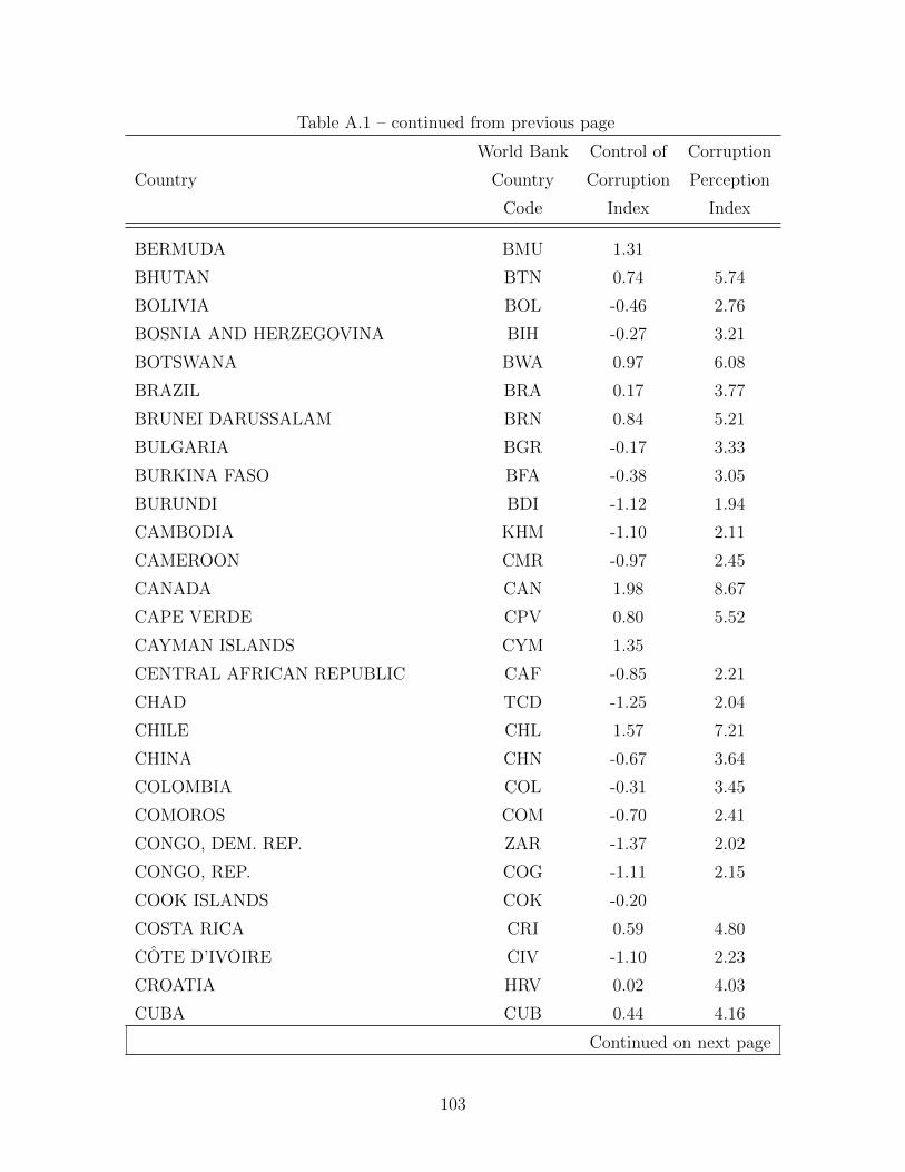
Table A.1 – continued from previous page
World Bank Control of Corruption
Country Country Corruption Perception
Code Index Index
BERMUDA BMU 1.31
BHUTAN BTN 0.74 5.74
BOLIVIA BOL -0.46 2.76
BOSNIA AND HERZEGOVINA BIH -0.27 3.21
BOTSWANA BWA 0.97 6.08
BRAZIL BRA 0.17 3.77
BRUNEI DARUSSALAM BRN 0.84 5.21
BULGARIA BGR -0.17 3.33
BURKINA FASO BFA -0.38 3.05
BURUNDI BDI -1.12 1.94
CAMBODIA KHM -1.10 2.11
CAMEROON CMR -0.97 2.45
CANADA CAN 1.98 8.67
CAPE VERDE CPV 0.80 5.52
CAYMAN ISLANDS CYM 1.35
CENTRAL AFRICAN REPUBLIC CAF -0.85 2.21
CHAD TCD -1.25 2.04
CHILE CHL 1.57 7.21
CHINA CHN -0.67 3.64
COLOMBIA COL -0.31 3.45
COMOROS COM -0.70 2.41
CONGO, DEM. REP. ZAR -1.37 2.02
CONGO, REP. COG -1.11 2.15
COOK ISLANDS COK -0.20
COSTA RICA CRI 0.59 4.80
COTE D’IVOIRE CIV -1.10 2.23
CROATIA HRV 0.02 4.03
CUBA CUB 0.44 4.16
Continued on next page
103
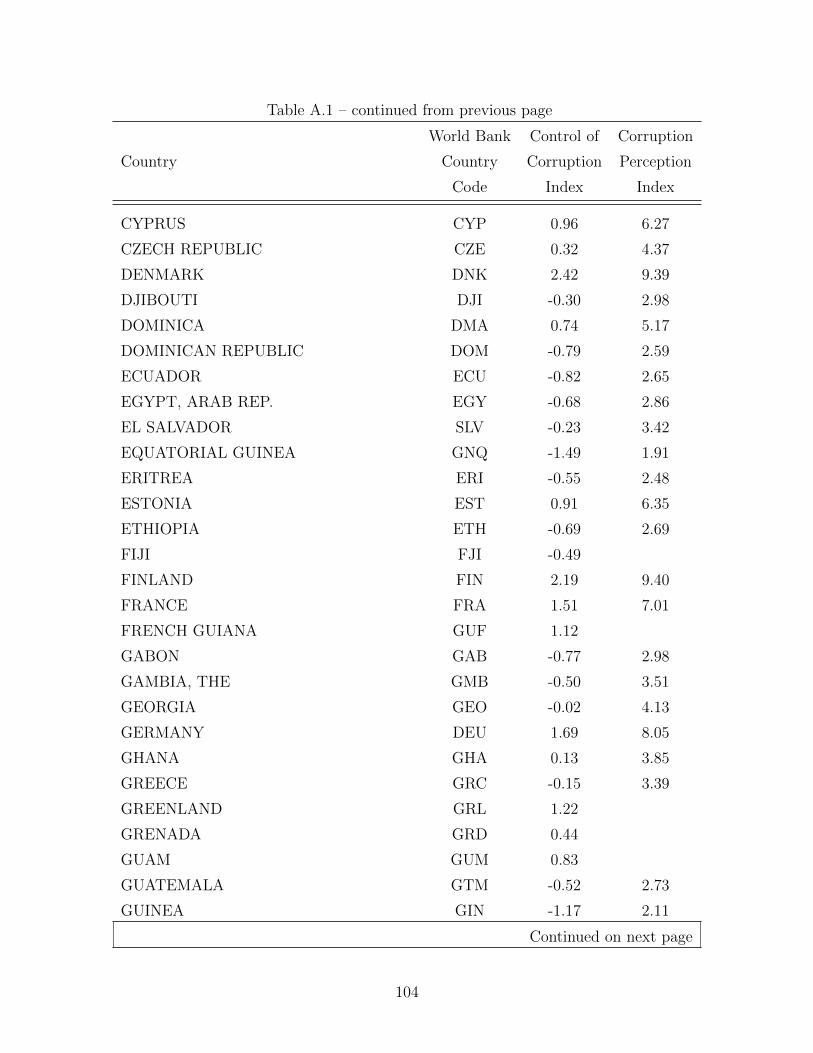
Table A.1 – continued from previous page
World Bank Control of Corruption
Country Country Corruption Perception
Code Index Index
CYPRUS CYP 0.96 6.27
CZECH REPUBLIC CZE 0.32 4.37
DENMARK DNK 2.42 9.39
DJIBOUTI DJI -0.30 2.98
DOMINICA DMA 0.74 5.17
DOMINICAN REPUBLIC DOM -0.79 2.59
ECUADOR ECU -0.82 2.65
EGYPT, ARAB REP. EGY -0.68 2.86
EL SALVADOR SLV -0.23 3.42
EQUATORIAL GUINEA GNQ -1.49 1.91
ERITREA ERI -0.55 2.48
ESTONIA EST 0.91 6.35
ETHIOPIA ETH -0.69 2.69
FIJI FJI -0.49
FINLAND FIN 2.19 9.40
FRANCE FRA 1.51 7.01
FRENCH GUIANA GUF 1.12
GABON GAB -0.77 2.98
GAMBIA, THE GMB -0.50 3.51
GEORGIA GEO -0.02 4.13
GERMANY DEU 1.69 8.05
GHANA GHA 0.13 3.85
GREECE GRC -0.15 3.39
GREENLAND GRL 1.22
GRENADA GRD 0.44
GUAM GUM 0.83
GUATEMALA GTM -0.52 2.73
GUINEA GIN -1.17 2.11
Continued on next page
104
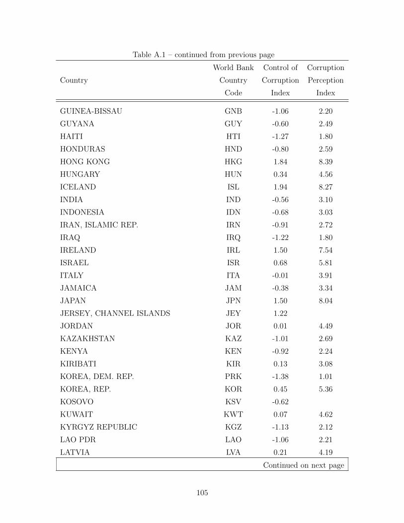
Table A.1 – continued from previous page
World Bank Control of Corruption
Country Country Corruption Perception
Code Index Index
GUINEA-BISSAU GNB -1.06 2.20
GUYANA GUY -0.60 2.49
HAITI HTI -1.27 1.80
HONDURAS HND -0.80 2.59
HONG KONG HKG 1.84 8.39
HUNGARY HUN 0.34 4.56
ICELAND ISL 1.94 8.27
INDIA IND -0.56 3.10
INDONESIA IDN -0.68 3.03
IRAN, ISLAMIC REP. IRN -0.91 2.72
IRAQ IRQ -1.22 1.80
IRELAND IRL 1.50 7.54
ISRAEL ISR 0.68 5.81
ITALY ITA -0.01 3.91
JAMAICA JAM -0.38 3.34
JAPAN JPN 1.50 8.04
JERSEY, CHANNEL ISLANDS JEY 1.22
JORDAN JOR 0.01 4.49
KAZAKHSTAN KAZ -1.01 2.69
KENYA KEN -0.92 2.24
KIRIBATI KIR 0.13 3.08
KOREA, DEM. REP. PRK -1.38 1.01
KOREA, REP. KOR 0.45 5.36
KOSOVO KSV -0.62
KUWAIT KWT 0.07 4.62
KYRGYZ REPUBLIC KGZ -1.13 2.12
LAO PDR LAO -1.06 2.21
LATVIA LVA 0.21 4.19
Continued on next page
105
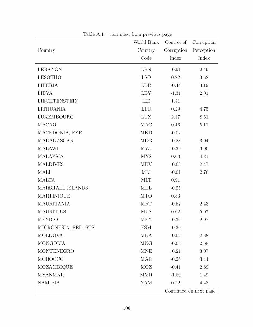
Table A.1 – continued from previous page
World Bank Control of Corruption
Country Country Corruption Perception
Code Index Index
LEBANON LBN -0.91 2.49
LESOTHO LSO 0.22 3.52
LIBERIA LBR -0.44 3.19
LIBYA LBY -1.31 2.01
LIECHTENSTEIN LIE 1.81
LITHUANIA LTU 0.29 4.75
LUXEMBOURG LUX 2.17 8.51
MACAO MAC 0.46 5.11
MACEDONIA, FYR MKD -0.02
MADAGASCAR MDG -0.28 3.04
MALAWI MWI -0.39 3.00
MALAYSIA MYS 0.00 4.31
MALDIVES MDV -0.63 2.47
MALI MLI -0.61 2.76
MALTA MLT 0.91
MARSHALL ISLANDS MHL -0.25
MARTINIQUE MTQ 0.83
MAURITANIA MRT -0.57 2.43
MAURITIUS MUS 0.62 5.07
MEXICO MEX -0.36 2.97
MICRONESIA, FED. STS. FSM -0.30
MOLDOVA MDA -0.62 2.88
MONGOLIA MNG -0.68 2.68
MONTENEGRO MNE -0.21 3.97
MOROCCO MAR -0.26 3.44
MOZAMBIQUE MOZ -0.41 2.69
MYANMAR MMR -1.69 1.49
NAMIBIA NAM 0.22 4.43
Continued on next page
106
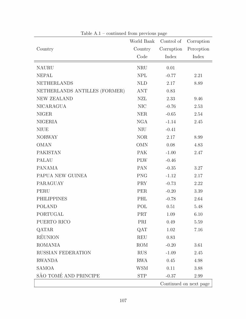
Table A.1 – continued from previous page
World Bank Control of Corruption
Country Country Corruption Perception
Code Index Index
NAURU NRU 0.01
NEPAL NPL -0.77 2.21
NETHERLANDS NLD 2.17 8.89
NETHERLANDS ANTILLES (FORMER) ANT 0.83
NEW ZEALAND NZL 2.33 9.46
NICARAGUA NIC -0.76 2.53
NIGER NER -0.65 2.54
NIGERIA NGA -1.14 2.45
NIUE NIU -0.41
NORWAY NOR 2.17 8.99
OMAN OMN 0.08 4.83
PAKISTAN PAK -1.00 2.47
PALAU PLW -0.46
PANAMA PAN -0.35 3.27
PAPUA NEW GUINEA PNG -1.12 2.17
PARAGUAY PRY -0.73 2.22
PERU PER -0.20 3.39
PHILIPPINES PHL -0.78 2.64
POLAND POL 0.51 5.48
PORTUGAL PRT 1.09 6.10
PUERTO RICO PRI 0.49 5.59
QATAR QAT 1.02 7.16
REUNION REU 0.83
ROMANIA ROM -0.20 3.61
RUSSIAN FEDERATION RUS -1.09 2.45
RWANDA RWA 0.45 4.98
SAMOA WSM 0.11 3.88
SAO TOME AND PRINCIPE STP -0.37 2.99
Continued on next page
107
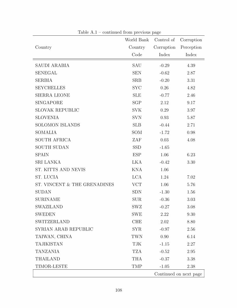
Table A.1 – continued from previous page
World Bank Control of Corruption
Country Country Corruption Perception
Code Index Index
SAUDI ARABIA SAU -0.29 4.39
SENEGAL SEN -0.62 2.87
SERBIA SRB -0.20 3.31
SEYCHELLES SYC 0.26 4.82
SIERRA LEONE SLE -0.77 2.46
SINGAPORE SGP 2.12 9.17
SLOVAK REPUBLIC SVK 0.29 3.97
SLOVENIA SVN 0.93 5.87
SOLOMON ISLANDS SLB -0.44 2.71
SOMALIA SOM -1.72 0.98
SOUTH AFRICA ZAF 0.03 4.08
SOUTH SUDAN SSD -1.65
SPAIN ESP 1.06 6.23
SRI LANKA LKA -0.42 3.30
ST. KITTS AND NEVIS KNA 1.06
ST. LUCIA LCA 1.24 7.02
ST. VINCENT & THE GRENADINES VCT 1.06 5.76
SUDAN SDN -1.30 1.56
SURINAME SUR -0.36 3.03
SWAZILAND SWZ -0.27 3.08
SWEDEN SWE 2.22 9.30
SWITZERLAND CHE 2.02 8.80
SYRIAN ARAB REPUBLIC SYR -0.97 2.56
TAIWAN, CHINA TWN 0.90 6.14
TAJIKISTAN TJK -1.15 2.27
TANZANIA TZA -0.52 2.95
THAILAND THA -0.37 3.38
TIMOR-LESTE TMP -1.05 2.38
Continued on next page
108
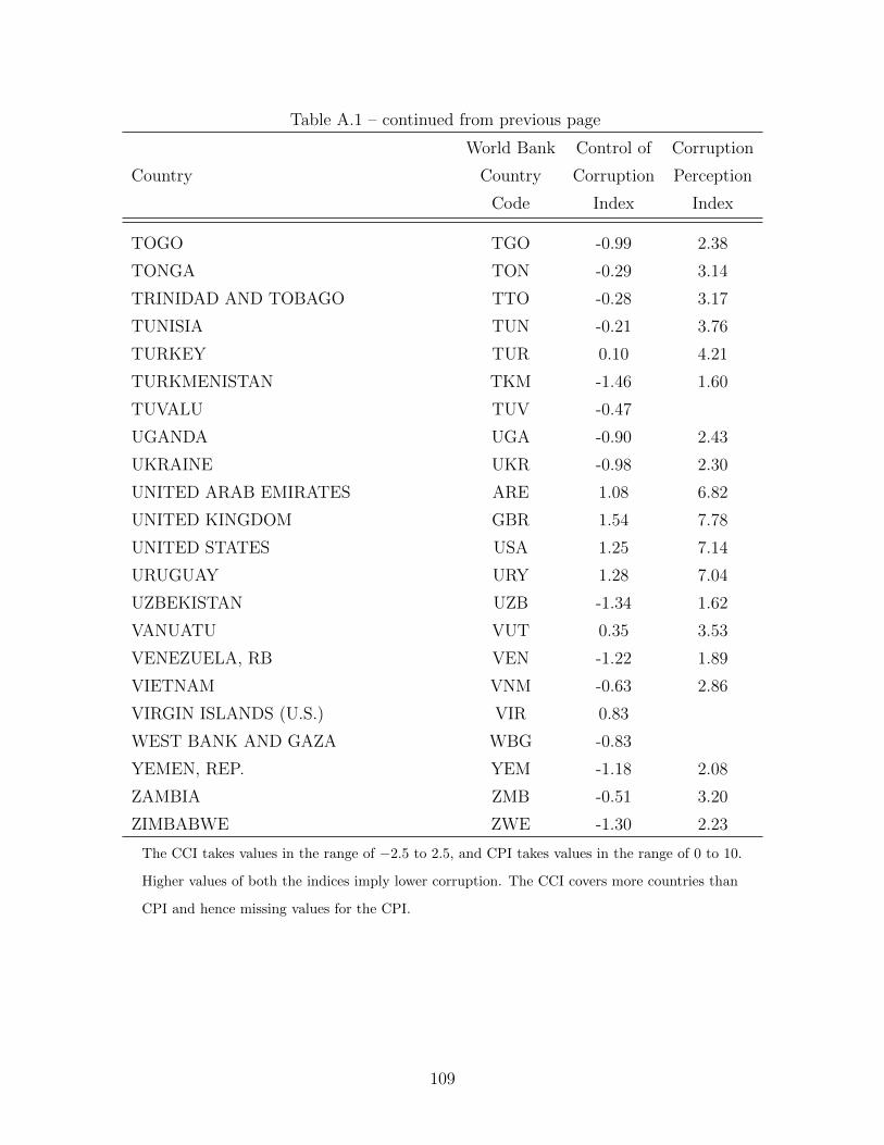
Table A.1 – continued from previous page
World Bank Control of Corruption
Country Country Corruption Perception
Code Index Index
TOGO TGO -0.99 2.38
TONGA TON -0.29 3.14
TRINIDAD AND TOBAGO TTO -0.28 3.17
TUNISIA TUN -0.21 3.76
TURKEY TUR 0.10 4.21
TURKMENISTAN TKM -1.46 1.60
TUVALU TUV -0.47
UGANDA UGA -0.90 2.43
UKRAINE UKR -0.98 2.30
UNITED ARAB EMIRATES ARE 1.08 6.82
UNITED KINGDOM GBR 1.54 7.78
UNITED STATES USA 1.25 7.14
URUGUAY URY 1.28 7.04
UZBEKISTAN UZB -1.34 1.62
VANUATU VUT 0.35 3.53
VENEZUELA, RB VEN -1.22 1.89
VIETNAM VNM -0.63 2.86
VIRGIN ISLANDS (U.S.) VIR 0.83
WEST BANK AND GAZA WBG -0.83
YEMEN, REP. YEM -1.18 2.08
ZAMBIA ZMB -0.51 3.20
ZIMBABWE ZWE -1.30 2.23
The CCI takes values in the range of −2.5 to 2.5, and CPI takes values in the range of 0 to 10.
Higher values of both the indices imply lower corruption. The CCI covers more countries than
CPI and hence missing values for the CPI.
109
Vita
Chandan Kumar Jha was born in Shri Khandhi Bhitha, a small and beautiful village
in the Indian state of Bihar, situated at the border of India and Nepal. He completed his
Bachelor of Arts in Economics from Magadh University in 2007 and earned a Masters of
Arts in Economics from Gokhale Institute of Politics and Economics in 2010. He began
pursuing the doctoral degree in Economics at Louisiana State University in Fall 2010 and
earned a Masters of Science in Economics in 2012 in the process. His primary research
focus is in the area of development economics and his current research topics include the
issues of corruption and gender inequality. He also contributes articles to Ideas for India, an
economics and policy portal and often writes Op-Eds on economic, social, and policy issues
for the Hindu Business Line, a leading Indian business daily.
110