essays on financial econometrics and derivatives pricing · the unifying themes of this...
TRANSCRIPT

2012-11
Mateusz P. DziubinskiPhD Thesis
Department of economics anD businessaarHus uniVersitY • DenmarK
essays on financial econometricsand Derivatives pricing

Essays on Financial Econometrics and Derivatives Pricing
By Mateusz P. Dziubinski
A dissertation submitted to
Business and Social Sciences, Aarhus University,
in partial fulfilment of the requirements of
the PhD degree in
Economics and Management


Contents
Preface v
Summary vii
Chapter 1. Option Valuation with the Simplied ComponentGARCH Model 1
Chapter 2. Conditionally-Uniform Feasible Grid SearchAlgorithm 25
Chapter 3. Commodity Derivatives Pricing with InventoryEects 57
iii


Preface
This PhD dissertation was written in the period from February 2008to February 2012 during my studies at the Department of Economicsand Business at Aarhus University. I am grateful to the departmentand to the Center for Research in Econometric Analysis of Time Series(CREATES), funded by the Danish National Research Foundation, forgenerous nancial support in connection with courses and conferences.I am further grateful to CREATES for providing excellent researchfacilities.
A number of people have contributed to the making of this thesis.I would like to express my sincere gratitude to my main advisor TimoTeräsvirta for providing guidance and numerous insightful commentsand suggestions throughout my PhD studies. I am grateful for havinghad the opportunity to work with my co-author Christian Bach on oneof the chapters. I hope we can continue our collaboration in the yearsto come.
At Aarhus University I would like to thank the faculty and fel-low students. I would also like to thank CREATES, Department ofEconomics and Business, Department of Mathematics, and ComputerScience Department for providing outstanding courses, seminars, con-ferences, and support. Special thanks also to Steen Thorbjørnsen forshowing me that stochastic processes can be easy and Svend Erik Gra-versen for revealing the mysteries of stochastic calculus to me and evenspending his free time doing so.
At the Department of Economics and Business I would like tothank my fellow PhD students for providing me with a welcoming,friendly environment and opportunities to discuss economics, nanceand (un)related topics. Christian deserves my gratitude for sharing anoce with me and providing me with endless opportunities for conver-sation, debate and learning relevant to our common interests. Finally,I would like to thank Anders for accompanying me on our individualyet common journey in the probability theory wonderland.
Last but not least, I would like to thank my family for their con-tinuing love and support.
Mateusz "Matt" P. Dziubinski, Aarhus, February 2012.
v

vi PREFACE
The predefense was held on March 21, 2012. I would like to thankthe members of the assessment committee, Peter Christoersen, OlafPosch (chair), and Lars Stentoft for their comments and suggestionsfor improvements. Most of those have been incorporated into the dis-sertation.
Mateusz "Matt" P. Dziubinski, Aarhus, July 2012.

Summary
The unifying themes of this dissertation are nancial econometricsand derivatives pricing. An underlying topic is the price behavior of anancial asset, be it a stock market index or a commodity derivative,with an additional focus on the factors aecting this behavior, like thevolatility and inventory levels. Practical implementation issues arisingin applying the models, together with an empirical motivation for thewhy are emphasized over a purely theoretical model treatment anddevelopment or the sole focus on the how.
The thesis contains three independent chapters, of which the rsttwo can be viewed as contributions to nancial econometrics, whereasthe third chapter has to do with derivatives pricing. In the rst chapter,entitled "Option Valuation with the Simplied Component GARCHModel", I introduce the Simplied Component GARCH (SCGARCH)option pricing model, show and discuss sucient conditions for non-negativity of the conditional variance, apply the model to both low-frequency and high-frequency nancial data, and consider the optionvaluation, comparing the model performance with similar models fromthe literature. Two volatility components in my model allow me tosatisfactorily model time structure of volatility.
The SCGARCH model builds on Engle and Lee (1999), Heston andNandi (2000), and Christoersen et al. (2008) (hereafter referred to asCJOW) models. Engle and Lee (1999) introduced the volatility com-ponent model in the GARCH context, while Heston and Nandi (2000)introduced a model with a closed-form solution for the European calloption-pricing formulas. The CJOW model is a generalization of theHeston and Nandi model allowing for a time-varying long-run com-ponent. The SCGARCH model is a simplied variant of the CJOWmodel, in which the non-negativity of the conditional variance is en-sured.
In the second chapter, entitled "Conditionally-Uniform FeasibleGrid Search Algorithm", I present and evaluate a numerical optimiza-tion method (together with an algorithm for choosing the startingvalues) pertinent to the constrained optimization problem where thevariables have to satisfy a sequentially dependent set of constraints.In practice, these arise (for instance) in the estimation of the modelswith inequality constraints, in particular GARCH models such as theEngle and Lee (1999) GARCH model and the Simplied Component
vii

viii Summary
GARCH (SCGARCH) model. The numerical optimization method, theConditionally-Uniform Feasible Grid Search (CUFGS), is essentially aparticular kind of a random grid search coupled with a constrainedfeasible Sequential Quadratic Programming (SQP) algorithm.
One of the reasons for developing it are the problems encounteredwhen using non-specialized gradient-based algorithms due to con-strained feasible space requirement and scaling. For example, in rela-tion to the Broyden-Fletcher-Goldfarb-Shanno (BFGS) algorithm, pop-ular among econometricians, Nocedal and Wright (2006) write:
(1) BFGS updating is generally less eective for constrained prob-
lems than in the unconstrained case because of the requirement
of maintaining a positive denite approximation to an under-
lying matrix that often does not have this property.(2) SQP methods are most ecient if the number of active con-
straints is nearly as large as the number of variables, that is,
if the number of free variables is relatively small. They re-
quire few evaluations of the functions, in comparison with aug-
mented Lagrangian methods, and can be more robust on badly
scaled problems.
I also provide the objective function and analytical gradient com-putation algorithms for the SCGARCH model, which are useful for thepractical implementation purposes.1
In the third chapter, "Commodity Derivatives Pricing with In-ventory Eects" (written jointly with Christian Bach), we introducetractable models for commodity derivatives pricing with inventory andvolatility eects, introduce a new, maturity-wise calibration methodcompatible with these models and apply it to modeling the commodityderivatives associated with the crude oil market.
The role of inventories in explaining price and volatility of com-modities has been studied in several papers. Brennan (1958) and Telser(1958) are early studies on the eect of the level of inventory on agricul-tural commodities, but the inventory eect has also been documentedfor metals (Ng and Pirrong (1994)) and oil and natural gas markets(Geman and Ohana (2009)). Instead of relying on a proxy for inven-tory data, we use weekly data on oil inventories. Geman and Nguyen(2005) construct a database of soybean inventory over a 10-year periodand show that volatility can be written as an exact inverse functionof inventory. In this chapter we do not nd such a clear relationship,
1To implement MLE in practice it is useful to have the analytical gradient.There are at least two reasons for that. First, in case of GARCH models estimationusing gradient-based optimization the analytical gradient is more accurate than itsnumerical approximation, see (Zivot, 2009, Section 5.1) and Brooks et al. (2001).Second, it may also be applied for computing the outer-product gradient (OPG)estimate of the information matrix.

Summary ix
although we see strong signs of the relationship between inventory andvolatility being negative.
We contribute to the existing literature in several respects. First,whereas the previous literature uses futures data for investigating therelationship between inventory and volatility, we use the informationavailable in options traded on futures. Second, performance assessmentin the previous literature has primarily evolved around explaining mo-ments of data or forecasting prices of futures. Instead, we asses theperformance of our model by considering both its ability of explain-ing prices in-sample and out-of-sample assessing both the pricing-performance and the hedging-performance of the models. Third, wemodel the futures surface rather than the spot price process, and limitthe number of parameters to calibrate (using the observed inventoryprocess instead of a latent one). We introduce a new, maturity-wise cal-ibration method compatible with this modeling methodology. Fourth,we use actual data on inventories rather than a proxy. Fifth, our modelis very exible and allows for analyzing several dierent types of rela-tionships between inventory and volatility.


Bibliography
Brennan, M. J. (1958). The supply of storage. The American Economic
Review 48 (1), 5072.Brooks, C., S. P. Burke, and G. Persand (2001). Benchmarks andthe accuracy of GARCH model estimation. International Journal ofForecasting 17 (1), 45 56.
Christoersen, P., K. Jacobs, C. Ornthanalai, and Y. Wang (2008).Option valuation with long-run and short-run volatility components.Journal of Financial Economics 90 (3), 272297.
Engle, R. F. and G. G. J. Lee (1999). A permanent and transi-tory component model of stock return volatility. In R. F. Engleand H. White (Eds.), Cointegration, Causality, and Forecasting: A
Festschrift in Honuor of Clive W.J. Granger, pp. 475497. OxfordUniversity Press.
Geman, H. and V. Nguyen (2005). Soybean inventory and forwardcurve dynamics. Management Science 51 (7), 10761091.
Geman, H. and S. Ohana (2009). Forward curves, scarcity and pricevolatility in oil and natural gas markets. Energy Economics 31 (4),576585.
Heston, S. and S. Nandi (2000). A closed-form GARCH option valua-tion model. Review of Financial Studies 13 (3), 585625.
Ng, V. K. and S. C. Pirrong (1994). Fundamentals and volatility:Storage, spreads, and the dynamics of metals prices. The Journal ofBusiness 67 (2), 20330.
Nocedal, J. and S. Wright (2006). Numerical optimization (second ed.).Springer: Springer.
Telser, L. G. (1958). Futures trading and the storage of cotton andwheat. Journal of Political Economy 66 (3), 233255.
Zivot, E. (2009). Practical issues in the analysis of univariate GARCHmodels. In T. G. Andersen, R. A. Davis, J.-P. Kreiÿ, and T. Mikosch(Eds.), Handbook of Financial Time Series, pp. 113155. Springer.
xi


CHAPTER 1
Option Valuation with the Simplied Component
GARCH Model
1
OPTION VALUATION WITH THE SIMPLIFIEDCOMPONENT GARCH MODEL
MATT P. DZIUBINSKI
Abstract. We introduce the Simplied Component GARCH (SC-GARCH) option pricing model, show and discuss sucient condi-tions for non-negativity of the conditional variance, apply it tolow-frequency and high-frequency nancial data, and consider theoption valuation, comparing the model performance with simi-lar models from the literature. Two volatility components in ourmodel, short-term and long-term, allow us to model time-structureof volatility.
JEL Classication. G12, C32.
1. Introduction
In this paper we introduce a discrete-time volatility model in whichthe conditional variance of the underlying asset follows a particularGARCH process. Our model can be used for option pricing, while twovolatility components allow us to model time structure thereof.
The model builds on Engle and Lee (1999), Heston and Nandi (2000)and Christoersen et al. (2008) (hereafter referred to as CJOW) mod-els. The model by Engle and Lee (1999) introduced the volatility com-ponent model in the GARCH context, while Heston and Nandi (2000)introduced a model with a closed-form solution for the European calloption-pricing formulas. The CJOW model is a generalization of theHeston and Nandi model allowing for a time-varying long-run com-ponent. Our model is a simplied specication of the CJOW model,which solves the problem of ensuring the non-negativity of the condi-tional variance.
Date: August 7, 2012.2000 Mathematics Subject Classication. Primary 37M10, 62M10, 91B84; Sec-
ondary 62P05.Key words and phrases. Stochastic volatility, volatility components, GARCH,
option pricing.We wish to thank Timo Teräsvirta for a discussion regarding non-negativity con-
ditions. We acknowledge nancial support by the Center for Research in Economet-ric Analysis of Time Series, CREATES, funded by the Danish National ResearchFoundation. All errors, omissions and mistakes are author's own responsibility.
2

OPTION VALUATION WITH THE SCGARCH MODEL 3
The paper proceeds as follows. In Section 2 we provide basic deni-tions and notation. We introduce the model in Section 3 (in which wealso discuss the non-negativity conditions), and discuss the estimationthereof in Section 4. In Section 5 we present the estimation results.Section 6 is devoted to option pricing, and, nally, Section 7 containsour conclusions.
2. Basic Definitions and Notation
We assume as given a probability space (Ω,F , P ) and a ltration F =(Ft)t∈T, where, depending on the context, we shall assume T = Z+ orT = Z ∩ [0, T ], T > 0 or T = Z ∩ [−1, T ], T ≥ 0. We refer to P as thephysical probability measure and we call (Ω,F ,F, P ) a ltered physicalprobability space. We shall also use probability measure Q on (Ω,F)and refer to it as the risk-neutral probability measure.
A stochastic process X on (Ω,F , P ) is a collection of R-valued randomvariables (Xt)t∈T, and we denote it by X = (Xt)t∈T.
The process X is said to be adapted if Xt ∈ Ft ∀t ∈ T (that is, it is Ftmeasurable for each t ∈ T).
The process X is said to be predictable if Xt ∈ Ft−1 ∀t ∈ T, and wedenote this by X ∈ P .The process X is said to be (F, P )-white noise with mean µX and
variance σ2X , writtenX
P∼ WN(µX , σ2X) if and only if, under probability
measure P , X has mean µX ∈ R and covariance function γ(s, t) =σ2Xδ|t−s|, where δh := 10(h) is the Kronecker delta and σ2
X ∈ R++.
The process X is said to be (F, P )-Gaussian white noise with mean
µX and variance σ2X , written X
P∼ GWN(µX , σ2X) if and only if X
P∼WN(µX , σ
2X) and Xt
P∼ N (µX , σ2X) ∀t ∈ T.
First-order partial dierential operator with respect to x is denoted ∂x.
For further details regarding stochastic processes and time series werefer the reader to Protter (2005) and Brockwell and Davis (1991).
3. The Model
We begin by presenting the SCGARCH and the CJOW models. Theadvantages of the CJOW model are the existence of a (quasi-)closed-form solution for the option pricing formulas, improved ability to modelthe smirk and the path of spot volatility and, distinctively, the ability tomodel the volatility term structure for details, see Christoersen et al.(2008). A problem with this model is that the volatility components
4 MATT P. DZIUBINSKI
may admit negative values. This leads to a contradiction in the contextof conditional variance modeling, as the conditional variance cannot benegative. We propose the SCGARCH model as a more parsimoniousmodel which solves this problem and discuss its relation to the CJOWmodel. Furthermore, we shall consider the properties of the model anddiscuss the estimation of its parameters.
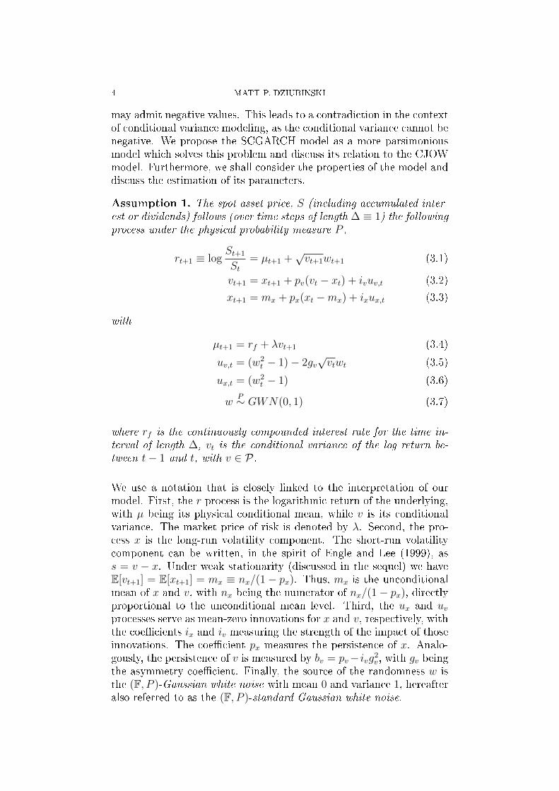
Assumption 1. The spot asset price, S (including accumulated inter-est or dividends) follows (over time steps of length ∆ ≡ 1) the followingprocess under the physical probability measure P ,
rt+1 ≡ logSt+1
St= µt+1 +
√vt+1wt+1 (3.1)
vt+1 = xt+1 + pv(vt − xt) + ivuv,t (3.2)
xt+1 = mx + px(xt −mx) + ixux,t (3.3)
with
µt+1 = rf + λvt+1 (3.4)
uv,t = (w2t − 1)− 2gv
√vtwt (3.5)
ux,t = (w2t − 1) (3.6)
wP∼ GWN(0, 1) (3.7)
where rf is the continuously compounded interest rate for the time in-terval of length ∆, vt is the conditional variance of the log return be-tween t− 1 and t, with v ∈ P.
We use a notation that is closely linked to the interpretation of ourmodel. First, the r process is the logarithmic return of the underlying,with µ being its physical conditional mean, while v is its conditionalvariance. The market price of risk is denoted by λ. Second, the pro-cess x is the long-run volatility component. The short-run volatilitycomponent can be written, in the spirit of Engle and Lee (1999), ass = v − x. Under weak stationarity (discussed in the sequel) we haveE[vt+1] = E[xt+1] = mx ≡ nx/(1− px). Thus, mx is the unconditionalmean of x and v, with nx being the numerator of nx/(1− px), directlyproportional to the unconditional mean level. Third, the ux and uvprocesses serve as mean-zero innovations for x and v, respectively, withthe coecients ix and iv measuring the strength of the impact of thoseinnovations. The coecient px measures the persistence of x. Analo-gously, the persistence of v is measured by bv = pv− ivg2
v , with gv beingthe asymmetry coecient. Finally, the source of the randomness w isthe (F, P )-Gaussian white noise with mean 0 and variance 1, hereafteralso referred to as the (F, P )-standard Gaussian white noise.

OPTION VALUATION WITH THE SCGARCH MODEL 5
3.1. Non-Negativity of the Conditional Variance. First, we shalllook at the CJOW model and consider the issues regarding the non-negativity of the conditional variance arising in its application.
3.1.1. CJOWModel. First, recall that Christoersen et al. (2008) modelcan be rewritten in our notation, replacing (3.6) with
ux,t = (w2t − 1)− 2gx
√vtwt (3.8)
and keeping the remaining equations intact.
The problem with this specication is that there is no guarantee onnon-negativity of v and since v is the conditional variance process, wearrive at a possible contradiction. In order to examine the seriousnessof the problem, we perform a simulation study and analyze the behaviorof the model.
3.1.2. CJOWModel Simulation Study. We perform a simulation studyto examine the behavior of this model performing a grid search withrespect to px searching from 0.0 to 1.0 with a step size of 0.001. Wedo this both for the original CJOW model and a deterministic versionthereof (i.e. the one where the driving noise process is assumed tobe identically equal to zero instead of a standard GWN), xing all theother parameter values to those in Table 1 in Christoersen et al. (2008)(for convenience, we reproduce it in Table 1) in addition setting rfto 1.000× 10⁻¹. We choose this particular parameter value, since it isthe one used by Christoersen et al. (2008) to dierentiate between theComponent and the Persistent Component (px = 1) models. Further-more, the reason we consider the unit interval as the parameter rangeis that for px < 0 non-negativity issues arise immediately (as we shallshow later on), while px > 1 leads to non-stationarity (in particular,the explosiveness of x and, consequently, v). For purposes of this study,T = Z ∩ [0, T ], T = 1, 000.
We divide the set of px coecient values into invalid and valid values,where the invalid ones are those that lead to negative values of v. Wend that the low parameter values are invalid, while the higher onesare valid the boundary being at approximately 0.9. This means forall px < 0.9 in our simulation study there exists a t(px) ∈ T such
that vt(px) < 0. Note, that in practice this leads to v1/2t(px) returning

6 MATT P. DZIUBINSKI
T = 1,000 Simulationrf 1.000× 10⁻¹
λ 2.092× 10+0
nx 8.208× 10−7
iv 1.580× 10−6
ix 2.480× 10−6
pv 6.437× 10−1
px 9.896× 10−1
gv 4.151× 10+2
gx 6.324× 10+1
Table 1. The coecient values used for the CJOWmodel simulation study.
NaN1 for the IEEE 7542 conforming architecture. Since commonlyapplied optimization routines will reject arguments leading to NaNs(or terminate with an error, leading to restarting the optimization withdierent starting values), this potentially explains the estimate of px =0.9896 obtained by Christoersen et al. (2008), which is very close to1. Hence, due to this numerical property of the model, one cannotnecessarily infer high persistence to hold in this case. This is becausethe high estimate might well be a numerical artifact, as opposed tobeing an empirical property of the data described by the model.
In addition, as we change the sample size T , the boundary value in-creases as the sample size increases. A possible interpretation of thisnding is that as the model runs for a longer time (i.e., as we have moredraws in the generated sample) the chance of drawing at least one neg-ative value increases. However, this is not solely due to Gaussianity ofw, because we obtain similar result for the deterministic version of themodel (i.e. even for a biased forecast) in fact, the boundary is higherfor the deterministic case than the stochastic one.
3.1.3. CJOW Model Discussion. We shall now proceed as follows:assuming the CJOW model, we rewrite (3.2) and (3.3), substituting(3.5) and (3.8), respectively:
vt+1 = xt+1 + pv(vt − xt) + iv((w2
t − 1)− 2gv√vtwt
)(3.9)
xt+1 = nx + pxxt + ix((w2
t − 1)− 2gx√vtwt
)(3.10)
1The term NaN stands for Not a Number. Here it results from applying thesquare root function to argument outside its domain, due to attempt to take thesquare root of a negative number.
2IEEE Standard 754 is a oating-point arithmetic standard, the most commonoating-point representation of real numbers today on computers for further ref-erence, see IEEE Task P754 (2008).
OPTION VALUATION WITH THE SCGARCH MODEL 7
where
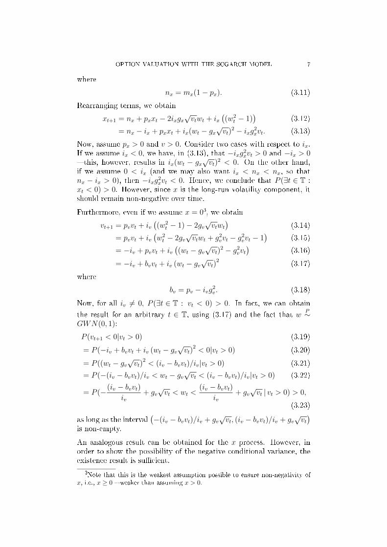
nx = mx(1− px). (3.11)
Rearranging terms, we obtain
xt+1 = nx + pxxt − 2ixgx√vtwt + ix
((w2
t − 1))
(3.12)
= nx − ix + pxxt + ix(wt − gx√vt)
2 − ixg2xvt. (3.13)
Now, assume px > 0 and v > 0. Consider two cases with respect to ix.If we assume ix < 0, we have, in (3.13), that −ixg2
xvt > 0 and −ix > 0 this, however, results in ix(wt − gx
√vt)
2 < 0. On the other hand,if we assume 0 < ix (and we may also want ix < nx < nx, so thatnx − ix > 0), then −ixg2
xvt < 0. Hence, we conclude that P (∃t ∈ T :xt < 0) > 0. However, since x is the long-run volatility component, itshould remain non-negative over time.
Furthermore, even if we assume x = 03, we obtain
vt+1 = pvvt + iv((w2
t − 1)− 2gv√vtwt
)(3.14)
= pvvt + iv(w2t − 2gv
√vtwt + g2
vvt − g2vvt − 1
)(3.15)
= −iv + pvvt + iv((wt − gv
√vt)
2 − g2vvt)
(3.16)
= −iv + bvvt + iv (wt − gv√vt)
2(3.17)
where
bv = pv − ivg2v . (3.18)
Now, for all iv 6= 0, P (∃t ∈ T : vt < 0) > 0. In fact, we can obtain
the result for an arbitrary t ∈ T, using (3.17) and the fact that wP∼
GWN(0, 1):
P (vt+1 < 0|vt > 0) (3.19)
= P (−iv + bvvt + iv (wt − gv√vt)
2< 0|vt > 0) (3.20)
= P ((wt − gv√vt)
2< (iv − bvvt)/iv|vt > 0) (3.21)
= P (−(iv − bvvt)/iv < wt − gv√vt < (iv − bvvt)/iv|vt > 0) (3.22)
= P (−(iv − bvvt)iv
+ gv√vt < wt <
(iv − bvvt)iv
+ gv√vt | vt > 0) > 0,
(3.23)
as long as the interval(−(iv − bvvt)/iv + gv
√vt, (iv − bvvt)/iv + gv
√vt)
is non-empty.
An analogous result can be obtained for the x process. However, inorder to show the possibility of the negative conditional variance, theexistence result is sucient.
3Note that this is the weakest assumption possible to ensure non-negativity ofx, i.e., x ≥ 0 weaker than assuming x > 0.

8 MATT P. DZIUBINSKI
We conclude that assuming a non-zero skewness parameter gx leads toa model that can result in negative values for the volatility components.
Note, that this is an inherent problem of the CJOW model per se in particular, this is not merely a peripheral problem limited to agiven particular numerical treatment of the model (as in, for instance,particular discretization schemes applied to the Heston model). Thisalso implies that the numerical optimization problem arising in theestimation of the CJOWmodel will, in general, be an ill-posed problem,due to inherent numerical instability associated with the presence ofthe NaN results on the IEEE 754 conforming architecture.
3.1.4. Heston-Nandi GARCH(2,2) model. Christoersen et al. (2004,Section 4.2) provide the mapping between CJOW and Heston-NandiGARCH(2,2). We can write the conditional variance in the componentmodel as a Heston-Nandi GARCH(2,2) process.
rt+1 = rf + λht+1 +√ht+1zt+1 (3.24)
ht+1 = w + b1ht + b2ht−1 + a1(zt − c1
√ht)
2 + a2(zt−1 − c2
√ht−1)2
(3.25)
zP∼ GWN(0, 1) (3.26)
where
a1 = iv + ix (3.27)
a2 = −(pxiv + pvix) (3.28)
b1 = (px + pv)−(ivgv + ixgx)
2
a1
(3.29)
b2 =−(pxivgv + pvixgx)
2
a2
− pxpv (3.30)
c1 =gviv + gxix
a1
(3.31)
c2 = −pxgviv + pvgxixa2
(3.32)
w = (nx − ix)(1− pv)− iv(1− px) (3.33)
Note that we can easily ensure non-negativity of the conditional vari-ance in the HN-GARCH(2,2) model (HN) imposing (sucient) condi-tions given by the following inequality constraints:
w > 0, b1 > 0, b2 > 0, a1 > 0, a2 > 0 (3.34)
As such, the original, unrestricted HN model does not suer from thelack of simple non-negativity conditions. In contrast, nonlinear param-eter restrictions (3.27)(3.33) are precisely what makes it quite dicult
OPTION VALUATION WITH THE SCGARCH MODEL 9
to come up with sensible constraints in particular, note that restric-tions (3.47)-(3.49) (derived in the following section, operating under theadditional assumption of gx = 0, also desirable for the interpretationof the model) would imply that a2 < 0 (with the sign of a1 inverselyrelated to the sign of a2) and make the signs of b1 and b2 dependent ona relation analogous to (3.49). This illustrates the trade-o betweenthe CJOW and the HN models although Christoersen et al. (2004,Section 4.2) argue that coming up with sensible parameter startingvalues (in the estimation context) and the stationarity requirements issimpler in the CJOW model compared to the HN model, it is easier toobtain simple non-negativity constraints in the HN model, as in (3.34).
Here, we oer an alternative approach, allowing us to proceed with amodel with a structure similar to CJOW (thus preserving the ease ofstarting values interpretation and simple stationarity conditions) withan additional benet of also having relatively simple non-negativityconditions.
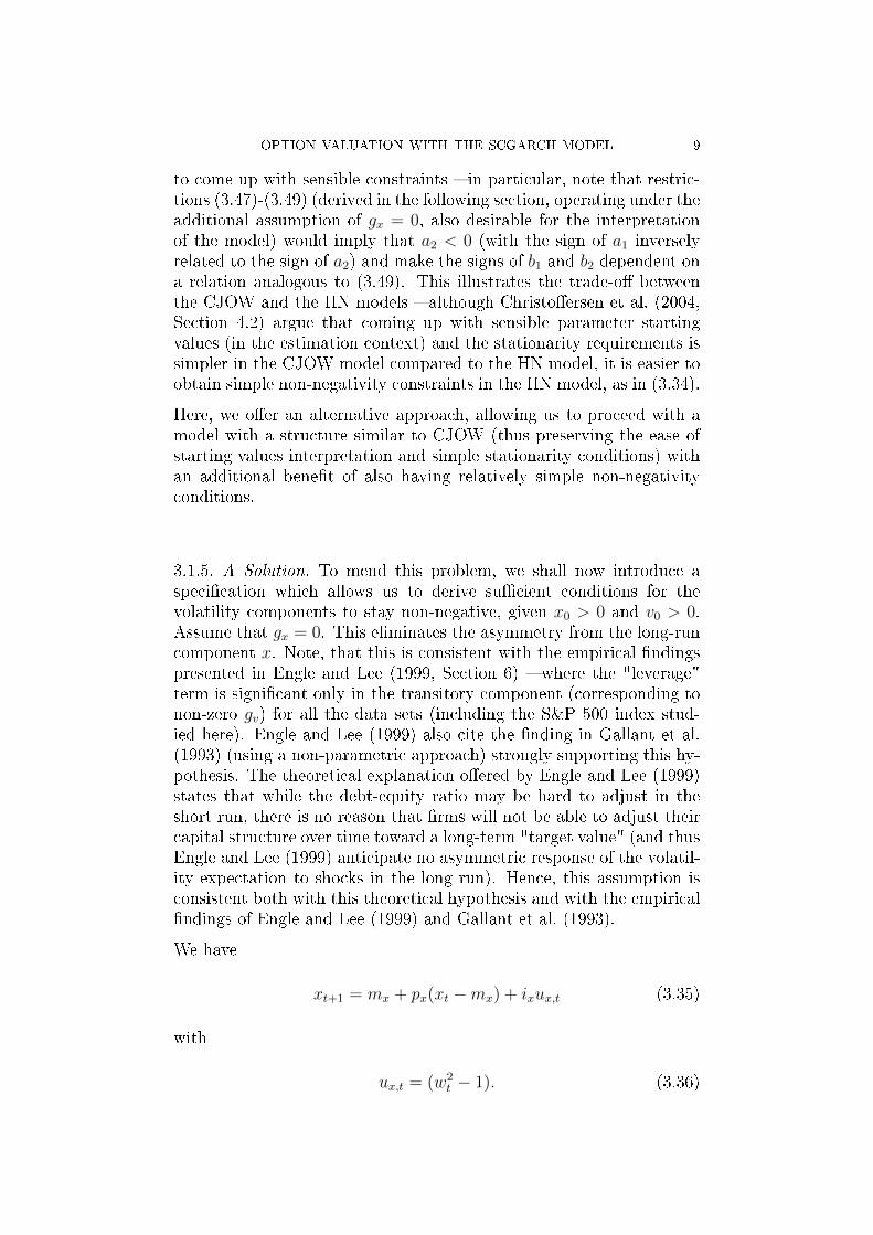
3.1.5. A Solution. To mend this problem, we shall now introduce aspecication which allows us to derive sucient conditions for thevolatility components to stay non-negative, given x0 > 0 and v0 > 0.Assume that gx = 0. This eliminates the asymmetry from the long-runcomponent x. Note, that this is consistent with the empirical ndingspresented in Engle and Lee (1999, Section 6) where the "leverage"term is signicant only in the transitory component (corresponding tonon-zero gv) for all the data sets (including the S&P 500 index stud-ied here). Engle and Lee (1999) also cite the nding in Gallant et al.(1993) (using a non-parametric approach) strongly supporting this hy-pothesis. The theoretical explanation oered by Engle and Lee (1999)states that while the debt-equity ratio may be hard to adjust in theshort run, there is no reason that rms will not be able to adjust theircapital structure over time toward a long-term "target value" (and thusEngle and Lee (1999) anticipate no asymmetric response of the volatil-ity expectation to shocks in the long run). Hence, this assumption isconsistent both with this theoretical hypothesis and with the empiricalndings of Engle and Lee (1999) and Gallant et al. (1993).
We have
xt+1 = mx + px(xt −mx) + ixux,t (3.35)
with
ux,t = (w2t − 1). (3.36)

10 MATT P. DZIUBINSKI
Rearranging (3.35) and substituting (3.36) we obtain
xt+1 = mx(1− px) + pxxt + ix(w2t − 1) (3.37)
= nx − ix + pxxt + ixw2t (3.38)
where
nx = mx(1− px). (3.39)
Note, that (3.38) follows the GMACH(1, 1) model by Yang and Bewley(1995)4. Now, in order to obtain non-negative values of x, we neednx > ix > 0 and px > 0. Furthermore, under weak stationarity (forwhich we also need |px| < 1) we have
E[xt+1] = mx ≡nx
1− px. (3.40)
This motivates our previous notation mx for the unconditional meanof x.
Inserting (3.38) and (3.5) into (3.2) yields:
vt+1 = xt+1 + pv(vt − xt) + ivuv,t (3.41)
= nx − ix + pxxt + ixw2t
+ pv(vt − xt) + ivuv,t (3.42)
= nx − ix + pxxt + ixw2t
+ pv(vt − xt) + iv((w2
t − 1)− 2gv√vtwt
). (3.43)
Rearranging terms and using pv = bv + ivg2v we have
vt+1 = nx − ix + pxxt + ixw2t
+ (bv + ivg2v)(vt − xt) + iv
(w2t − 1− 2gv
√vtwt
)(3.44)
= (nx − ix − iv) + (px − bv − ivg2v)xt + ixw
2t
+ bvvt + iv(w2t − 2gv
√vtwt + ivg
2v
)(3.45)
= (nx − ix − iv) + (px − pv)xt + bvvt
+ ixw2t + iv (wt − gv
√vt)
2(3.46)
Now, assuming bv > 0, iv > 0 and ix > 0, we have a sucient conditionfor non-negativity of v, which is (nx − ix − iv) + (px − pv)x > 0. Sincewe have already established conditions for non-negativity of x, we needto ensure that in addition to them, (nx − ix − iv) > 0, (px − pv) > 0and bv > 0. Thus, the joint sucient conditions for non-negativity of
4This is similar to assuming c = 0 in the model by Heston and Nandi (2000) ina way that we also obtain GMACH(1, 1) dynamics.

OPTION VALUATION WITH THE SCGARCH MODEL 11
the volatility components v and x are as follows:
px ≤ 1, bv > 0, iv > 0, ix > 0 (3.47)
nx > ix + iv (3.48)
px > pv > ivg2v > 0 (3.49)
Restrictions in (3.47) are analogous to those in Engle and Lee (1999).Note, that similarly to Engle and Lee (1999) we also assume that theweak stationarity restriction px < 1 holds. The economic interpre-tation of (3.48) is that the mean long-term volatility level has to besuciently high relative to the strength of the innovation impact (re-call from (3.40) that nx is the numerator of the unconditional mean,i.e. mx ≡ nx/(1− px)). The interpretation of (3.49), which can also bestated as px > bv > 0, is that the persistence of the long-run componenthas to be higher than the one of the short-run component and that theimpact of the innovation(s) to the short-run component cannot be asstrong as to outweigh the persistence.
Hereafter we shall denote our parameter vector by
θ := (rf , λ, nx, iv, ix, pv, px, gv)T
and the restricted parameter space
Θ := θ ⊆ Θ : (3.47)− (3.49),
where Θ ⊆ Rp, p = 8.
4. Maximum Likelihood Estimation
We shall now derive a Maximum Likelihood Estimator (MLE)5 for ourmodel. For notational convenience we assume that the sample includesan observation for t = 0. Hereafter we shall assume that non-negativityconditions (3.47)(3.49) hold.
First, note that by the assumptions (3.1)(3.7) we have that wP∼
GWN(0, 1) and v ∈ P . Using this and (3.1) yields rt|Ft−1P∼ N (µt, vt).
Hence, the conditional probability density function (PDF) of rt|Ft−1 is
f(rt|Ft−1) =1√2πvt
exp
(−(rt − µt)2
2vt
). (4.1)
5The kind of MLE we derive is called the conditional MLE in Hayashi (2000) see pp. 547549.

12 MATT P. DZIUBINSKI
Using (3.1) again and simplifying we obtain
f(rt|Ft−1) =1√2πvt
exp
(−(√vtwt)
2
2vt
)(4.2)
=1√2πvt
exp
(−vtw
2t
2vt
)(4.3)
=1√2πvt
exp
(−w
2t
2
). (4.4)
Now, we can formulate our MLE in terms of an M-estimator. If thePDFs are parametrized by a parameter vector θ then the M-estimatorusing the log-likelihood of the sample over t = 0, 1, ..., N can be writtenas:
θ = arg maxθ∈Θ
Qn(θ) (4.5)
Qn(θ) =1
N
N∑
t=0
`t(θ) (4.6)
`t(θ) = log f(rt|Ft−1; θ) (4.7)
= −1
2log(2π)− 1
2log(vt)−
1
2w2t . (4.8)
Note, that using proportional and monotonic transformations, we canstate our problem for the purposes of minimization as follows:
θ = arg minθ∈Θ
Qn(θ) (4.9)
Qn(θ) =N∑
t=0
lt(θ) (4.10)
lt(θ) = log(vt) + w2t . (4.11)
For the numerical details, including objective function computationalgorithm and analytical gradient formulas, we refer the reader to Dz-iubinski (2010).
5. Estimation Results
Due to the results in Dziubinski (2010) we choose Conditionally-UniformFeasible Grid Search (CUFGS) with Feasible Sequential Quadratic Pro-gramming (FSQP) to estimate the models. FSQP allows us to solve theconstrained optimization problem (4.9), while coupling it with CUFGSenables us to widen the search space thus increasing the chance ofconvergence.

OPTION VALUATION WITH THE SCGARCH MODEL 13
We use the S&P 500 index data to calculate the (log) returns. Wet our model to both daily (source: Yahoo Finance, period 1/3/19507/22/2009) and high-frequency (5-minute) data (source: Price-Data.comS&P 500, period 4/21/198212/6/2007 from Price-Data.com). For thepurposes of research reproducibility, we use the same starting valuesas the ones in the column Estimation Starting Values in Table 1 inDziubinski (2010).6
We have considered three methods of obtaining the standard errors the OPG method, the numerical Hessian, and the sandwich estimator.Since there are numerical issues present when inverting the numericalHessian (even if it is obtained using analytical rst derivatives), wechoose to report the OPG standard errors. 7
Note that looking at the estimates for two data sets sampled at dierentfrequencies is a way to empirically investigate temporal aggregationproperties of our model. See Zivot (2009, Section 3.4) for a discussionof temporal aggregation in a context of GARCH models.
The estimates obtained using the FSQP-AL CUFGS optimization algo-rithm8 appear in Table 2. The problems with the large standard errors(causing insignicance) were practically not encountered in case of theFSQP optimization (where we used sandwich estimation and only usedOPG or Hessian errors in case of numerical problems; the only problemwas with a NaN gv standard error in low-frequency data). This conrmsour belief that the choice of the optimization method matters a greatdeal. Unsurprisingly, as in the similar models in the term-structurecomponents GARCH literature, there are still some issues with esti-mating λ and gv. The persistence seems to be slightly lower in case ofthe low-frequency data (coecients pv and px) note, however, thatequality of pv and px means that CUFGS yielded px to be optimal atthe lower corner solution. Furthermore, pv constitutes the lower boundfor px generated by CUFGS.
The results for the FSQP-NL CUFGS optimization algorithm in Table3 are mostly similar to those discussed above. It can be seen (looking
6Note, that as Zivot (2009) reports, a poor choice of starting values can lead toan ill-behaved log-likelihood and cause convergence problems, which is why we usethe starting values that satisfy the non-negativity conditions.
7As an alternative, one could also use analytical Hessian. In fact, Fiorentiniet al. (1996) and Hafner and Herwartz (2008) report, in the context of GARCHestimation, that the analytical Hessian signicantly outperforms the approximation.However, in our model, this comes at a cost of calculating 82 = 64 derivatives (or,
ensuring that the estimates θ remain in Θ and using Qn ∈ C2(Θ) with symmetry
due to Young's Theorem, 8(8+1)2 = 36 derivatives). Also, bootstrapping the errors
is a possibility.8For a discussion of the FSQP-AL and the FSQP-NL CUFGS optimization al-
gorithms see Dziubinski (2010).

14 MATT P. DZIUBINSKI
at the estimates and associated standard errors) that gv seems to beestimated more accurately in this case.
Daily Data 5-minute DataT 14, 984 523, 068rf 5.604× 10⁻⁴ (1.048× 10⁻⁴) 2.685× 10⁻¹⁰ (1.548× 10⁻⁶)
λ −7.024× 10⁻¹ (1.392× 10+0) −4.392× 10+0 (1.475× 10+0)nx 4.744× 10−6 (5.998× 10⁻⁷) 1.047× 10⁻⁷ (8.741× 10⁻⁹)
iv 2.320× 10⁻⁶ (4.376× 10⁻⁷) 2.742× 10⁻⁸ (1.785× 10−9)
ix 2.396× 10−6 (9.433× 10⁻⁷) 7.714× 10⁻⁸ (6.401× 10⁻⁹)pv 9.375× 10⁻¹ (3.896× 10⁻³) 9.157× 10⁻¹ (6.563× 10−3)px 9.375× 10−1 (7.828× 10⁻³) 9.157× 10⁻¹ (6.652× 10⁻³)gv 2.183× 10+2 (NaN) 1.595× 10+1 (1.247× 10+2)
Qn(θ) −1.29423× 10+5 −6.7172× 10+6
Table 2. The estimates (standard errors in parenthe-ses) obtained for the S&P 500 data using FSQP-ALCUFGS optimization algorithm.
Daily Data 5-minute DataT 14, 984 523, 068rf 7.028× 10⁻⁴ (1.174× 10⁻⁴) 2.906× 10⁻²⁹ (1.540× 10⁻⁶)
λ −4.007× 10⁻¹ (1.488× 10+0) −3.913× 10+0 (1.465× 10+0)nx 4.040× 10−6 (8.989× 10⁻⁷) 1.049× 10⁻⁷ (2.714× 10⁻¹⁰)
iv 3.474× 10⁻⁶ (1.910× 10⁻⁸) 2.018× 10⁻¹⁰ (8.008× 10−5)
ix 5.336× 10−7 (1.097× 10⁻⁷) 1.047× 10⁻⁷ (8.008× 10⁻⁵)pv 9.460× 10⁻¹ (4.777× 10⁻³) 9.155× 10⁻¹ (1.350× 10−1)px 9.460× 10−1 (4.312× 10⁻²) 9.155× 10⁻¹ (1.784× 10⁻⁴)gv 1.022× 10+2 (4.339× 10+0) 5.031× 10+2 (9.509× 10+1)
Qn(θ) −1.29362× 10+5 −6.71722× 10+6
Table 3. The estimates (standard errors in parenthe-ses) obtained for the S&P 500 data using FSQP-NLCUFGS optimization algorithm.
6. Option Pricing
We shall consider option pricing under our model. In general, there areseveral approaches to look at:

OPTION VALUATION WITH THE SCGARCH MODEL 15
(1) CJOW risk-neutralization using the conditional moment gen-erating function (MGF), based on Christoersen et al. (2008)
(2) Monte-Carlo, Empirical Martingale Simulation (EMS), basedon Duan and Simonato (1998)
(3) Monte-Carlo, Empirical Martingale Correction (EMC), basedon Chorro et al. (2010)
(4) alternative risk-neutralization method,(5) dierent model specication and derivation of the pertinent
non-negativity conditions:(a) change the source of randomness w so that it follows a
distribution with positive support,(b) change the v and x specication, e.g. formulate the equa-
tions in log terms in the spirit of an EGARCH model.
The pricing formulas using the analytical methods might be harder toderive (and would often be infeasible in the case of exotic options).The disadvantage of the Monte-Carlo-based pricing methods might beslower performance and, besides, they might need further adjustmentto ensure the martingale property, see Duan and Simonato (1998) andChorro et al. (2010).
6.1. CJOW-MGF Approach. As our model is a simplication of theChristoersen et al. (2008) model we may, in principle, consider usingthe option-pricing formulas presented there. In practice, however, adiculty arises in attempts to apply them. In order to perform theoption valuation one needs to derive the moment generating function(MGF) for the component GARCH process (provided in Appendix Aof Christoersen et al. (2008)), specify the dynamics under the risk-neutral measure Q (provided in Appendix B of Christoersen et al.(2008)) and proceed with the option-valuation formula (given in section4.4 of Christoersen et al. (2008)). The problem arises in the secondstep, the risk-neutralization.
Following Christoersen et al. (2008) we need EQ[exp(rt+1)] = exp(rf ),which requires that
rt+1 ≡ logSt+1
St= µQt+1 +
√vt+1w
Qt+1 (6.1)
with
µQt+1 = rf −1
2vt+1. (6.2)
This in turn implies that
wQt+1 = wt+1 + (λ+1
2)√vt+1. (6.3)

16 MATT P. DZIUBINSKI
We also want to ensure the equality of the conditional variances underthe two measures:
VP [rt+1|Ft] = VQ[rt+1|Ft]. (6.4)
We therefore need to have equal variance innovations under the twomeasures that is
(wt − gi√vt)
2 = (wQt − gQi√vt)
2, i = v, x. (6.5)
This can be achieved by dening the risk-neutral parameters:
gQi = gi + λ+1
2, i = v, x. (6.6)
Now, the problem is that in our specication we have
gx = 0. (6.7)
Thus
gQx = λ+1
2. (6.8)
This means
gQx = 0 ⇐⇒ λ = −1
2. (6.9)
Hence, without restricting the market price of risk λ to a value whichis not particularly realistic, we cannot ensure that the Q-dynamic isgoing to remain such that we stay within our class of models (where wecan apply the sucient conditions for non-negativity of the conditionalvariance).
6.2. Empirical Martingale Simulation (EMS). EMS is a variance-reduction method ensuring the martingale property to be used withMonte Carlo pricing. The problem from our point of view is, how-ever, that the EMS relies on the formulation of the model under theQ measure that is, a prior risk-neutralization. However, our model(similarly to CJOW) is stated under the P measure, so analytical risk-neutralization would be required. But then, the one available method(CJOW, discussed above) is not applicable if we want to stay withinour class of models. This excludes the EMS from any further consid-erations.
6.3. Empirical Martingale Correction (EMC). The Empirical Mar-tingale Correction method is, in fact, inspired by the EMS, see Chorroet al. (2010). The fundamental dierence is that it is applicable tothe models stated under the P measure, such as ours. In this method,we make no assumption on the risk-neutralization (i.e. the shape ofthe pricing kernel, involving Radon-Nikodym derivative dQ
dP), and we
compute prices for options with time to maturity (T − t) by simulatingsampled paths of the stochastic model under the historical measure P.

OPTION VALUATION WITH THE SCGARCH MODEL 17
To rule out arbitrage opportunities, we directly impose risk neutralityconstraints. The ith sampled historical nal price for the underlying isdenoted by ST,i.
The Empirical Martingale Correction works such that the previouslysampled prices are replaced by:
ST,i =ST,i
1N
∑Ni=1 ST,i
Ster(T−t). (6.10)
The sampled average of ST,i is exactly equal to Ster(T−t), that is, the
risk neutral conditional expectation. With this approach, we only shiftthe historical distribution in a way that prevents arbitrage opportuni-ties by implicitly changing the drift of this distribution. Chorro et al.(2010) compare this approach with the ane Stochastic Discount Fac-tor (SDF) methodology in Cochrane (2002) and nd that the pricesobtained by these two methods are close to each other.
6.4. Option Pricing Results. Finally, we compare the option pricingresults in our model with those in the Black-Scholes-Merton modeland Heston-Nandi GARCH(1, 1) model (HN). In this section we usedaily data only. For comparison, we consider option pricing underthe SCGARCH model using the estimates obtained using FSQP-ALand FSQP-NL (applying CUFGS in both cases). We estimate the HNmodel using fOptions R package for details, see Wuertz (2007). Theestimation results are shown in Table 4.
N = 14,984 Daily Dataλ 3.451× 10+0
ω 1.139× 10−281
α 3.671× 10⁻⁶
β 9.005× 10⁻¹
γ 1.196× 10+2
Log-Likelihood 88559.65Persistence 0.953Variance 7.806764× 10⁻⁵
Table 4. The estimates obtained for the S&P 500 dailydata: the HN model.
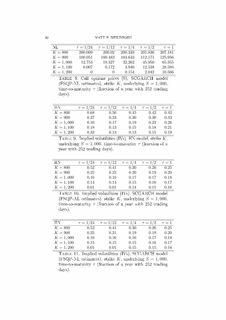
We present the pricing results across moneyness and maturity in Tables58, with implied volatilities (IVs) reported in Tables 911.
Note that Hull and White (1987) nd that the Black and Scholes (1973)model tends to overprice at-the-money (ATM) options and underprice
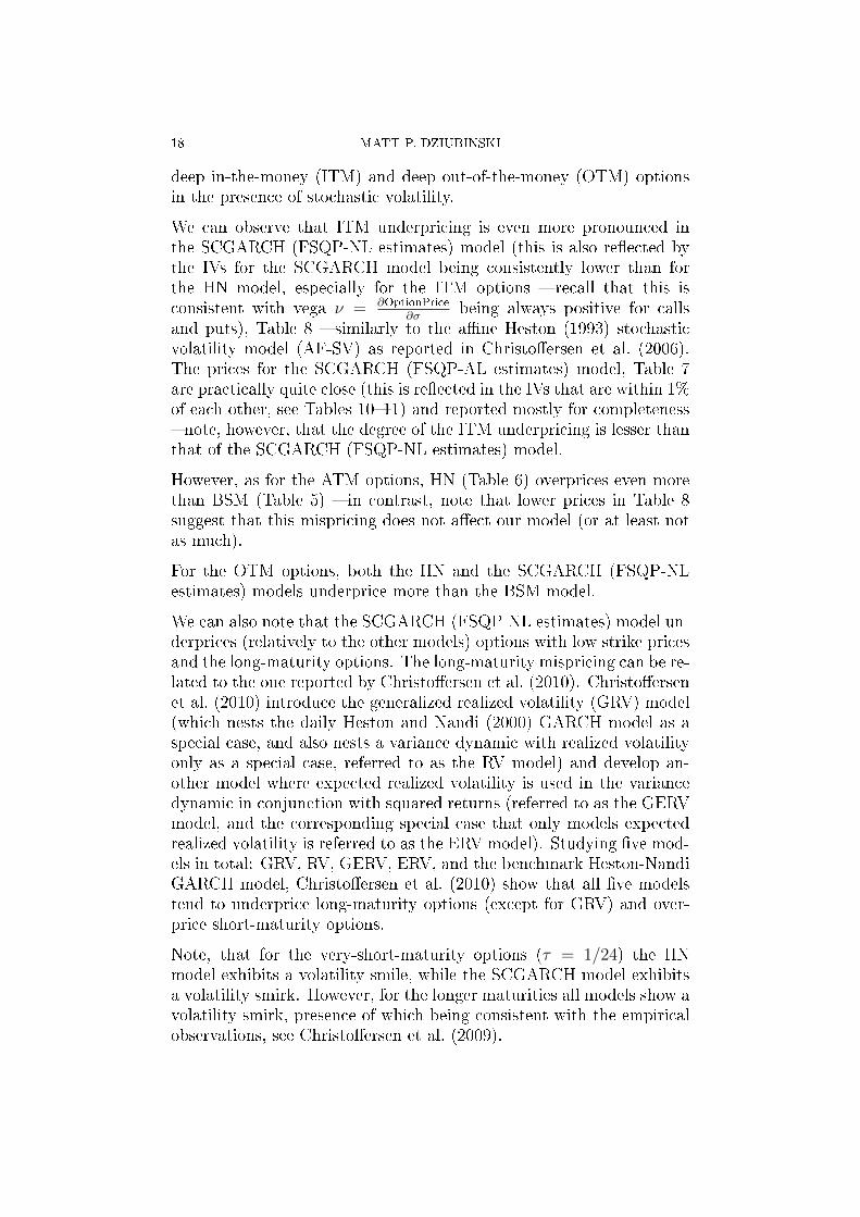
18 MATT P. DZIUBINSKI
deep in-the-money (ITM) and deep out-of-the-money (OTM) optionsin the presence of stochastic volatility.
We can observe that ITM underpricing is even more pronounced inthe SCGARCH (FSQP-NL estimates) model (this is also reected bythe IVs for the SCGARCH model being consistently lower than forthe HN model, especially for the ITM options recall that this isconsistent with vega ν = ∂OptionPrice
∂σbeing always positive for calls
and puts), Table 8 similarly to the ane Heston (1993) stochasticvolatility model (AF-SV) as reported in Christoersen et al. (2006).The prices for the SCGARCH (FSQP-AL estimates) model, Table 7are practically quite close (this is reected in the IVs that are within 1%of each other, see Tables 1011) and reported mostly for completeness note, however, that the degree of the ITM underpricing is lesser thanthat of the SCGARCH (FSQP-NL estimates) model.
However, as for the ATM options, HN (Table 6) overprices even morethan BSM (Table 5) in contrast, note that lower prices in Table 8suggest that this mispricing does not aect our model (or at least notas much).
For the OTM options, both the HN and the SCGARCH (FSQP-NLestimates) models underprice more than the BSM model.
We can also note that the SCGARCH (FSQP-NL estimates) model un-derprices (relatively to the other models) options with low strike pricesand the long-maturity options. The long-maturity mispricing can be re-lated to the one reported by Christoersen et al. (2010). Christoersenet al. (2010) introduce the generalized realized volatility (GRV) model(which nests the daily Heston and Nandi (2000) GARCH model as aspecial case, and also nests a variance dynamic with realized volatilityonly as a special case, referred to as the RV model) and develop an-other model where expected realized volatility is used in the variancedynamic in conjunction with squared returns (referred to as the GERVmodel, and the corresponding special case that only models expectedrealized volatility is referred to as the ERV model). Studying ve mod-els in total: GRV, RV, GERV, ERV, and the benchmark Heston-NandiGARCH model, Christoersen et al. (2010) show that all ve modelstend to underprice long-maturity options (except for GRV) and over-price short-maturity options.
Note, that for the very-short-maturity options (τ = 1/24) the HNmodel exhibits a volatility smile, while the SCGARCH model exhibitsa volatility smirk. However, for the longer maturities all models show avolatility smirk, presence of which being consistent with the empiricalobservations, see Christoersen et al. (2009).

OPTION VALUATION WITH THE SCGARCH MODEL 19
BSM τ = 1/24 τ = 1/12 τ = 1/4 τ = 1/2 τ = 1K = 800 202.266 204.526 213.506 226.904 253.488K = 900 102.550 105.127 116.270 133.473 165.920K = 1, 000 12.882 19.098 36.996 57.901 93.228K = 1, 100 0.005 0.199 4.848 16.757 43.962K = 1, 200 8× 10⁻¹⁰ 6× 10⁻⁵ 0.236 3.168 17.390
Table 5. Call options prices ($), BSM model, strike K,underlying S = 1, 000, time-to-maturity τ (fraction of ayear with 252 trading days).
HN τ = 1/24 τ = 1/12 τ = 1/4 τ = 1/2 τ = 1K = 800 202.209 204.527 213.628 227.459 254.714K = 900 102.495 105.334 117.605 135.623 168.677K = 1, 000 12.970 19.667 38.187 59.816 96.081K = 1, 100 0.069 0.078 3.711 15.900 44.827K = 1, 200 0.068 3× 10⁻⁶ 0.052 2.041 16.403
Table 6. Call options prices ($), HN model, strike K,underlying S = 1, 000, time-to-maturity τ (fraction of ayear with 252 trading days).
AL τ = 1/24 τ = 1/12 τ = 1/4 τ = 1/2 τ = 1K = 800 200.009 200.023 200.448 202.11 207.738K = 900 100.073 100.613 105.064 112.791 126.780K = 1, 000 12.816 18.429 32.530 46.404 66.046K = 1, 100 0.004 0.127 3.768 12.513 28.883K = 1, 200 0 0 0.116 1.922 10.580
Table 7. Call options prices ($), SCGARCH model(FSQP-AL estimates), strike K, underlying S = 1, 000,time-to-maturity τ (fraction of a year with 252 tradingdays).
20 MATT P. DZIUBINSKI
NL τ = 1/24 τ = 1/12 τ = 1/4 τ = 1/2 τ = 1K = 800 200.009 200.02 200.348 201.836 207.181K = 900 100.051 100.483 104.643 112.171 125.956K = 1, 000 12.753 18.327 32.262 45.950 65.355K = 1, 100 0.007 0.172 3.946 12.538 28.594K = 1, 200 0 0 0.154 2.042 10.566
Table 8. Call options prices ($), SCGARCH model(FSQP-NL estimates), strike K, underlying S = 1, 000,time-to-maturity τ (fraction of a year with 252 tradingdays).
HN τ = 1/24 τ = 1/12 τ = 1/4 τ = 1/2 τ = 1K = 800 0.68 0.56 0.45 0.42 0.43K = 900 0.37 0.33 0.30 0.30 0.33K = 1, 000 0.16 0.17 0.19 0.22 0.26K = 1, 100 0.18 0.13 0.15 0.18 0.21K = 1, 200 0.33 0.13 0.13 0.15 0.19
Table 9. Implied volatilities (IVs), HN model, strikeK,underlying S = 1, 000, time-to-maturity τ (fraction of ayear with 252 trading days).
HN τ = 1/24 τ = 1/12 τ = 1/4 τ = 1/2 τ = 1K = 800 0.52 0.41 0.30 0.26 0.25K = 900 0.25 0.22 0.20 0.19 0.20K = 1, 000 0.16 0.16 0.17 0.17 0.18K = 1, 100 0.14 0.14 0.15 0.16 0.17K = 1, 200 0.01 0.01 0.14 0.15 0.16
Table 10. Implied volatilities (IVs), SCGARCH model(FSQP-AL estimates), strike K, underlying S = 1, 000,time-to-maturity τ (fraction of a year with 252 tradingdays).
HN τ = 1/24 τ = 1/12 τ = 1/4 τ = 1/2 τ = 1K = 800 0.52 0.41 0.30 0.26 0.25K = 900 0.25 0.21 0.19 0.19 0.20K = 1, 000 0.16 0.16 0.16 0.17 0.18K = 1, 100 0.15 0.15 0.15 0.16 0.17K = 1, 200 0.01 0.01 0.15 0.15 0.16
Table 11. Implied volatilities (IVs), SCGARCH model(FSQP-NL estimates), strike K, underlying S = 1, 000,time-to-maturity τ (fraction of a year with 252 tradingdays).

OPTION VALUATION WITH THE SCGARCH MODEL 21
One could add that another empirically interesting exercise would beto use the option prices in estimation, similarly to what Christoersenet al. (2008) suggested. Note, however, that in our model we do notuse analytical option pricing formulas, but instead apply a Monte-Carlomethod. On a single-core CPU (central processing unit) this methodis too slow to be used in this application. 9 A very promising ap-proach, however, would be to use parallelized many-core GPU (graph-ics processing unit) computation since MC is a so-called embarrass-ingly parallel problem, that would yield very signicant performanceimprovements. In particular, in an application of MC pricing involvingpath-dependent options, Joshi (2010) demonstrates that it is possibleto get accuracy of 2 × 10⁻⁴ in less than a ftieth of a second, con-cluding that GPU technology has rendered the Monte Carlo pricingof Asian options suciently fast that there is no longer any need foranalytic approximations. This approach would also make possible toinvestigate forecasting properties of the model.
7. Conclusions
This paper presents a discrete-time volatility model in which the un-derlying follows a process with conditional variance driven by the newSimplied Component GARCH process. It is a more parsimoniousmodel than the CJOW one and allows us to derive sucient conditionsfor non-negativity of the conditional variance.
Maximum likelihood estimation of the model is discussed.
We provide an empirical illustration, applying the model to the S&P500 index data. The results are consistent with our economic intuition.
We propose an option pricing method consistent with our model
9As a practical illustration, note the reported "0" prices for K = $1,200 optionsin Table 8. We believe these are numerical artifacts which result from the slowconvergence rate of the MC procedure while we have also obtained "0" prices evenfor K = $1,100 when using 1,000 MC iterations (which only took 4.3 s to compute),the results we report here have been obtained with 100,000 MC iterations, whichrequire over 120 min per table (each with 5 distinct strikes and 5 distinct maturities,giving 25 distinct options). Typically, S&P 500 data set containing 500 distinctoptions per day (with 100 distinct strikes ranging from $900 to $1,900 and 5 distinctmaturities of 15, 45, 75, 165, and 345 days) would require approximately 500
25 × 2 h= 40 h per 1 iteration of the optimization algorithm (since each iteration requiresoption pricing) for 1 day of data. With the average number of 750 iterations onewould expect total required execution time of approximately 30,000 h for 1 day ofdata. This underscores the fact that using single-core CPU is not enough for anempirically relevant estimation (with empirically relevant sample sizes) when usingthe MC pricing methods.

22 MATT P. DZIUBINSKI
The performance of the pricing method across moneyness and maturityis compared with that of the Heston-Nandi GARCH and Black-Scholes-Merton models. The results of the comparison suggest that our modelmight constitute a particularly interesting choice for the valuation ofthe ATM options.
Several of the future research directions and possible extensions tothis work are worth consideration regarding to the advanced grid-generation techniques and optimization algorithms and applications ofGPUs allowing for more advanced pricing and forecasting applications.We provide a number of approaches to achieve that in the respectivesections of this paper.
References
Brockwell, P. J. and R. A. Davis (1991): Time Series: Theoryand Methods, New York: Springer Verlag, 2nd ed.
Chorro, C., D. Guegan, and F. Ielpo (2010): Martingalizedhistorical approach for option pricing, Finance Research Letters, 7,2428.
Christoffersen, P., S. Heston, and K. Jacobs (2009): TheShape and Term Structure of the Index Option Smirk: Why Mul-tifactor Stochastic Volatility Models Work So Well, ManagementScience, 55, 19141932.
Christoffersen, P., K. Jacobs, B. Feunou, and N. Meddahi
(2010): The Economic Value of Realized Volatility, Working Paper.Christoffersen, P., K. Jacobs, and K. Mimouni (2006): AnEmpirical Comparison of Ane and Non-Ane Models for EquityIndex Options, Working Paper, McGill University.
Christoffersen, P., K. Jacobs, C. Ornthanalai, and
Y. Wang (2008): Option valuation with long-run and short-runvolatility components, Journal of Financial Economics, 90, 272297.
Christoffersen, P., K. Jacobs, and Y. Wang (2004): Op-tion Valuation with Long-run and Short-run Volatility Components,CIRANO Working Papers 2004s-56, CIRANO.
Cochrane, J. (2002): Asset Pricing, Princeton University Press.Duan, J.-C. and J.-G. Simonato (1998): Empirical MartingaleSimulation for Asset Prices, Management Science, 44, 12181233.
Dziubinski, M. P. (2010): Conditionally-Uniform Feasible GridSearch (CUFGS), CREATES Working Paper.
Engle, R. F. and G. G. J. Lee (1999): A Permanent and Transi-tory Component Model of Stock Return Volatility, in Cointegration,Causality, and Forecasting: A Festschrift in Honor of Clive W.J.Granger, University Press, 475497.

OPTION VALUATION WITH THE SCGARCH MODEL 23
Fiorentini, G., G. Calzolari, and L. Panattoni (1996): Ana-lytic Derivatives and the Computation of GARCH Estimates, Jour-nal of Applied Econometrics, 11, 399417.
Gallant, A. R., P. E. Rossi, and G. Tauchen (1993): NonlinearDynamic Structures, Econometrica, 871907.
Hafner, C. and H. Herwartz (2008): Analytical quasi maximumlikelihood inference in multivariate volatility models, Metrika, 67,219239.
Hayashi, F. (2000): Econometrics, Princeton University Press.Heston, S. and S. Nandi (2000): A closed-form GARCH optionvaluation model, Review of Financial Studies, 13, 585625.
Hull, J. C. and A. D. White (1987): The Pricing of Options onAssets with Stochastic Volatilities, Journal of Finance, 42, 281300.
IEEE Task P754 (2008): IEEE 754-2008, Standard for Floating-Point Arithmetic.
Joshi, M. (2010): Graphical Asian Options, Wilmott Journal, 2,97107.
Protter, P. E. (2005): Stochastic Integration and Dierential Equa-tions, Springer, 2nd ed.
Wuertz, D. (2007): fOptions: Financial Software Collection-fOptions. R package version 260.72, in Rmetrics.
Yang, M. and R. Bewley (1995): Moving average conditional het-eroskedastic processes, Economics Letters, 49, 367 372.
Zivot, E. (2009): Practical Issues in the Analysis of UnivariateGARCH Models, in Handbook of Financial Time Series, Springer,113155.
(Matt P. Dziubinski) CREATESSchool of Economics and Management
University of Aarhus
Building 1322, DK-8000 Aarhus C
Denmark
E-mail address, Matt P. Dziubinski: [email protected]


CHAPTER 2
Conditionally-Uniform Feasible Grid Search
Algorithm
25

CONDITIONALLY-UNIFORM FEASIBLE GRID
SEARCH ALGORITHM
MATT P. DZIUBINSKI
Abstract. We present and evaluate a numerical optimizationmethod (together with an algorithm for choosing the starting val-ues) pertinent to the constrained optimization problem where thevariables have to satisfy a sequentially dependent set of constraints.In practice, these arise (for instance) in the estimation of the mod-els with inequality constraints, in particular GARCH models suchas the Engle and Lee (1999) GARCH model and the SimpliedComponent GARCH (SCGARCH) model. We also provide algo-rithms for the objective function and analytical gradient compu-tation for SCGARCH. The method improves upon ad hoc modi-cations of unconstrained optimization algorithms (such as BFGSwith a penalized objective function) prevalent in practice and isfound to be more eective in nding the solution.
JEL Classication. C32, C51, C58, C61, C63, C88.
1. Introduction
In this paper we present a numerical optimization method applicable toconstrained optimization problems, where the variables have to satisfya sequentially dependent set (SDS) of constraints (i.e., the one involvingconstraints involving multiple variables, where a variable constrainedby a given relation is then involved in a subsequent constraint for an-other set of variables). The method, the Conditionally-Uniform Feasi-ble Grid Search (CUFGS), is essentially a particular kind of a randomgrid search coupled with a constrained feasible Sequential QuadraticProgramming (SQP) algorithm.
Date: August 7, 2012.2000 Mathematics Subject Classication. Primary 62F30, 65C60, 65Y20, 90C30,
90C55; Secondary 37M10, 62M10, 91B84.Key words and phrases. Constrained optimization, GARCH, infeasibility, infer-
ence under constraints, nonlinear programming, performance of numerical algo-rithms, SCGARCH, sequential quadratic programming.
We acknowledge nancial support by the Center for Research in Economet-ric Analysis of Time Series, CREATES, funded by the Danish National ResearchFoundation.
26

CONDITIONALLY-UNIFORM FEASIBLE GRID SEARCH ALGORITHM 27
We apply it to the estimation of the Engle and Lee (1999) GARCHmodel (hereafter referred to as EL) and the Simplied ComponentGARCH Model (SCGARCH) of Dziubinski (2011).
One of the reasons for developing it are the problems encounteredwhen using non-specialized (unconstrained) gradient-based optimiza-tion algorithms due to constrained feasible space requirement andscaling. For example, in relation to the Broyden-Fletcher-Goldfarb-Shanno (BFGS) algorithm, popular with econometricians, Nocedal andWright (2006) write:
(1) BFGS updating is generally less eective for constrained prob-lems than in the unconstrained case because of the requirementof maintaining a positive denite approximation to an underly-ing matrix that often does not have this property.
(2) SQP methods are most ecient if the number of active con-straints is nearly as large as the number of variables, that is,if the number of free variables is relatively small. They requirefew evaluations of the functions, in comparison with augmentedLagrangian methods, and can be more robust on badly scaledproblems.
Note that observation (2) in particular applies to the SCGARCHmodel,with 8 constraints and 8 variables.
As an unconstrained optimization algorithm, BFGS does not apply toconstrained optimization problems per se. However, it is often usedin conjunction with ad hoc modications (such as penalized objectivefunction), which are generally less eective. In addition, it is also nota good t for the badly scaled or highly constrained models (i.e., oneswhere the number of active constraints is nearly as large as the numberof variables) which is also often the case for the GARCH models withnon-negativity inequality constraints.
In contrast, our algorithm is specically designed for the SDS-constrainedoptimization problems. We illustrate its superior performance in twoapplications (estimation of two dierent GARCH models), both in aMonte Carlo study (with a known DGP, data-generating process) andon a real-world data (S&P 500 index returns). Another advantage ofthe CUFGS algorithm is that it be coupled with another algorithmother than FSQP (which extends it to the cases where the other op-timization method is known, but when one still faces the problem ofgenerating feasible starting values consistent with the constraints-SDS).In this study we focus on the CUFGS-FSQP coupling for empirical ap-plications.

28 MATT P. DZIUBINSKI
The paper proceeds as follows. In Section 2 we present the SCGARCHmodel and the Engle and Lee (1999) GARCH model. We discuss es-timation in Section 3. In Sections 4 and 5 we analyze the estimationalgorithms and show the results. Section 6 contains our conclusions.
In the Appendix, we also provide the objective function and analyticalgradient computation algorithms for SCGARCH, useful for the practi-cal implementation purposes.
2. The Models
For reference we present the SCGARH and the EL models; for detailssee Dziubinski (2011) and Engle and Lee (1999), respectively. Theobserved time-series (e.g., log return on the spot asset price), r follows(over time steps of length ∆ ≡ 1) the following process under the(physical) probability measure P ,
rt+1 ≡ logSt+1
St= µt+1 + εt+1 (2.1)
εt+1 =√vt+1wt+1 (2.2)
vt+1 = xt+1 + pv(vt − xt) + ivuv,t (2.3)
xt+1 = mx + px(xt −mx) + ixux,t (2.4)
with
µt+1 = rf + λvt+1 (2.5)
uv,t = (w2t − 1)− 2gv
√vtwt (2.6)
ux,t = (w2t − 1) (2.7)
wP∼ GWN(0, 1) (2.8)
where rf is the continuously compounded interest rate for the timeinterval of length ∆, vt is the conditional variance of the log returnbetween t − 1 and t, with v ∈ P . The process w is a Gaussian white
noise with mean 0 and variance 1, i.e., wtP∼ N (0, 1) ∀t ∈ T and w
P∼WN(0, 1) (under probability measure P , w has mean 0 and covariancefunction γ(s, t) = δ|t−s|, where δh := 10(h) is the Kronecker delta).
This model is a simplied specication of the Christoersen et al.(2008) model, solving the problem of ensuring non-negativity of theconditional variance. The sucient conditions for non-negativity ofvolatility components v and x are:
px ≤ 1, bv > 0, iv > 0, ix > 0 (2.9)
nx > ix + iv (2.10)
px > pv > ivg2v > 0 (2.11)

CONDITIONALLY-UNIFORM FEASIBLE GRID SEARCH ALGORITHM 29
We denote our parameter vector by
θSCGARCH := (rf , λ, nx, iv, ix, pv, px, gv)T
and the restricted parameter space by
ΘSCGARCH := θSCGARCH ⊆ ΘSCGARCH : (2.9)− (2.11),where ΘSCGARCH ⊆ RpSCGARCH , pSCGARCH = 8.
Now, we can obtain the Engle and Lee (1999) GARCH model fromthe SCGARCH model, replacing (2.5), (2.6), and (2.7) above with thefollowing:
µt+1 = rf (2.12)
uv,t = ε2t − xt (2.13)
ux,t = ε2t − vt (2.14)
The sucient conditions for non-negativity of volatility components vand x are:
0 > px ≤ 1, pv > 0, iv > 0, ix > 0, nx > 0 (2.15)
px > iv + pv > 0 (2.16)
pv > ix > 0 (2.17)
In this case, we denote our parameter vector by
θEL := (rf , nx, iv, ix, pv, px)T
and the restricted parameter space by
ΘEL := θEL ⊆ ΘEL : (2.15)− (2.17),where Θ ⊆ RpEL , pEL = 6.
Note that (2.15)-(2.17) involve two linear sequentially dependent con-straints, ix − pv < 0 and iv + pv − px < 0 in order to verify whetherpx satises its constraint one rst needs to know pv which must obeyits own constraint.
Constraints given by (2.9)-(2.11) involve three sequentially dependentconstraints (one non-linear and two linear, respectively): ivg
2v−pv < 0,
ix + iv − nx < 0, pv − px < 0 here, iv aects the rst two constraints(needed for pv and nx), while pv (from the rst constraint) is requiredto verify the subsequent constraint for px.
3. Maximum Likelihood Estimation
A statistical method used for estimating the models is the MaximumLikelihood Estimation (MLE), which involves maximizing an objectivefunction (called the (log)likelihood function) in order to obtain theestimates.

30 MATT P. DZIUBINSKI
Dziubinski (2011) shows that we can state our optimization problemas a constrained minimization problem:
θ = arg minθ∈Θ
QN(θ) (3.1)
QN(θ) =N∑
t=0
lt(θ) (3.2)
lt(θ) = log(vt) + w2t . (3.3)
where θ is a generic parameter specialized to θEL for the EL modeland to θSCGARCH for the SCGARCH model (with the rest of the entitiesspecialized analogously).
4. A Simulation Study of Estimation Method Choice
4.1. Overview. In this section we provide an overview of some of themethods to estimate the models under consideration.
We simulate each model using the coecient values given in Table 1(they are interesting in practice, since they have the same magnitude asthose in Table 1 of Dziubinski (2011)), omitting inapplicable parame-ters for the EL model, and estimate the parameters using the simulateddata and the following algorithms1:
(1) NM - Nelder-Mead(2) FR - Fletcher-Reeves(3) PR - Polak-Ribière(4) BFGS - Broyden-Fletcher-Goldfarb-Shanno(5) SA - Simulated Annealing(6) PG - Projected Gradient(7) SPG - Spectral Projected Gradient(8) FSQP - Feasible Sequential Quadratic Programming
The Nelder-Mead (also known as downhill simplex) algorithm is aderivative-free optimization method, FR and PR are nonlinear con-jugate gradient methods, BFGS is a quasi-Newton method. PG is anextension of the steepest descent method for unconstrained minimiza-tion, where a line search is performed over the direction of a projectedgradient. SPG is similar to PG, except accelerated convergence due tothe choice of the spectral step-length; see Birgin et al. (2000) for details.
1We use the implementations thereof provided by O2scl anobject-oriented library for numerical programming in C++ see:http://o2scl.sourceforge.net/. The exception is FSQP, which uses CF-SQP implementation see Lawrence et al. (1997).

CONDITIONALLY-UNIFORM FEASIBLE GRID SEARCH ALGORITHM 31
Simulation (DGP) Estimation Starting Valuesrf 1.000× 10⁻¹ 9.000× 10⁻²
λ 2.000× 10+0 1.800× 10+0
nx 8.000× 10−6 7.200× 10⁻⁶
iv 1.000× 10⁻⁶ 9.000× 10−7
ix 2.000× 10−6 1.800× 10⁻⁶
pv 6.000× 10⁻¹ 5.400× 10−1
px 9.000× 10−1 8.100× 10⁻¹
gv 4.000× 10+2 3.600× 10+2
Qn,SCGARCH −8.427097× 10+3 −6.228086× 10+3
Qn,EL −125, 348 −115, 476
Table 1. The coecient values used in the simulationstudy. Sample sizes NSCGARCH = 1,000 and NEL =15,000. Both in the simulation and in the estimationwe are omitting inapplicable parameters for the ELmodel.
SA is a probabilistic metaheuristic (convergence to an optimal solutionis not guaranteed) for the global derivative-free optimization. FSQPis a quadratic programming method applicable to the constrained op-timization problems. For the rst four algorithms, see Nocedal andWright (2006), for SA see Henderson et al. (2003) or Dreo et al. (2005),for PG see Kelley (1999) and for SPG see Birgin et al. (2000).
FSQP is based on Sequential Quadratic Programming (SQP), modiedso as to generate feasible iterates. Sequential quadratic programming(SQP) methods model the general constrained optimization problemby a quadratic programming subproblem at each iterate and denethe search direction to be the solution of this subproblem. It is im-portant to design the quadratic subproblem so that it yields a goodstep for the nonlinear optimization problem, see Nocedal and Wright(2006). A description of FSQP can be found in Lawrence et al. (1997).There are two FSQP algorithms: FSQP-AL and FSQP-NL. In theFSQP-AL (monotone line search), an Armijo type arc search (hencethe "A" in "FSQP-AL") is used with the property that the step of unitlength is eventually accepted, which is a requirement for superlinearconvergence. In the FSQP-NL algorithm the same eect is achievedby means of a nonmonotone search (hence the "N" in "FSQP-NL")along a straight line. In other words, in the FSQP-AL algorithm theobjective function decreases at each iteration, while in FSQP-NL wehave a decrease of the objective function within at most four iterations.For details, see Lawrence et al. (1997).
For reproducibility purposes, we use the default seed for the SimulatedAnnealing. To minimize the warm-up period we use the unconditional

32 MATT P. DZIUBINSKI
mean of v and x to initialize v0 and x0, that is, we set the startingvalues to mx derived from the starting values of nx and px.
Note, that McCullough and Renfro (1999) and Brooks et al. (2001)stress the importance of reporting the initial values provided to theGARCH estimation software. Without them, any conditional het-eroscedasticity model is only partially specied, because the elementson which the likelihood is conditioned are not specied if the initial val-ues are not given. McCullough and Renfro (1999) also report that theinitialization of the series, though often overlooked, can substantiallyaect the solution produced by the software.
4.2. Constraints. In practice we may actually need a constrainedminimization algorithm in order to ensure that the non-negativity con-ditions hold. Only the last three algorithms in our list are of this type(note, that PG and SPG only allow for hypercubic constraints, whileFSQP allows for nonlinear functional constraints).
A solution commonly used in practice, see for example in Rouah andVainberg (2007), is to implement a penalty, so that violating non-negativity conditions generates a large value of the objective function.For the methods requiring this modication, we adjust the algorithmsas follows:
Penalized-Objective-Function l(N, θ, w, v, x, r)Input: a parameter vector θ, starting values r0, v0, x0
Output: the objective function l ≡∑Nt=0 lt(θ)
1 if Positivity-Conditions(θ) 6= TRUE
2 then return Penalty
3 l ← Summand l0(θ, w, v, x, r)4 for t← 0 to (N − 1) do5 l← l + Summand lt+1(θ, w, v, x, r)6 return l
Penalized-Gradient ∇l(N, θ, w, v, x, r)Input: a parameter vector θ, starting values r0, v0, x0
Output: the gradient g ≡ ∇l(θ)1 if Positivity-Conditions(θ) 6= TRUE
2 then return Penalty
3 l ← Summand l0(θ, w, v, x, r)4 g ← Summand ∇l0(θ, w, v, x, r)5 for t← 0 to (N − 1) do6 l← l + Summand lt+1(θ, w, v, x, r)7 g ← g + Summand ∇lt+1(θ, w, v, x, r)8 return g

CONDITIONALLY-UNIFORM FEASIBLE GRID SEARCH ALGORITHM 33
The boolean expression Positivity-Conditions(θ) is TRUE ⇐⇒θ ∈ Θ, and FALSE otherwise. Analogously to Rouah and Vainberg(2007), Penalty is assumed constant and large enough to have the or-der of magnitude larger than the objective function evaluated at start-ing values.
4.3. Results with the known DGP optimization study for the
SCGARCH model. For the SCGARCH model the maximum num-ber of iterations is 1,000 in all of the cases2 The sample size N = 1, 000.
NM FR PRrf = 9.000× 10−2 = 9.000× 10−2 = 9.000× 10⁻²
λ 2.800× 10+0 = 1.800× 10+0 = 1.800× 10+0
nx = 7.200× 10⁻⁶ 7.673× 10⁻⁶ 7.671× 10⁻⁶
iv = 9.000× 10⁻⁷ 4.946× 10⁻¹³ 3.834× 10⁻¹⁴
ix = 1.800× 10⁻⁶ 2.786× 10⁻⁶ 2.748× 10⁻⁶
pv = 5.400× 10−1 = 5.400× 10−1 = 5.400× 10⁻¹
px = 8.100× 10−1 = 8.100× 10−1 = 8.100× 10⁻¹
gv = 3.600× 10+2 = 3.600× 10+2 = 3.600× 10+2
Time (s) 0.0× 10+0 1.3439× 10+2 1.34516× 10+2
Qn(θ) −6.244133× 10+3 −6.747140× 10+3 −6.741407× 10+3
Table 2. The estimated coecient values obtained inthe estimation study using NM, FR and PR. Penaltyset to 999, 999.999. Symbol = indicates that the valuesare equal to the initial values.
We use the starting values reported in the third column (denoted Esti-mation Starting Values) of Table 1. The results are reported in Tables2 and 3. We notice that almost every unconstrained optimization al-gorithm performs unsatisfactorily. This may be due to the dicultyensuring that the estimates remain in Θ. The Penalty encountered inthis case introduces non-smoothness of the objective function, whereasmany of the algorithms require smoothness for convergence. Similarly,Zivot (2009) reports that the GARCH log-likelihood function is not
2The reason for choosing this criterion as opposed to, say, maximum elapsedtime, is to ensure the reproducibility of the results, independent of the performanceof the computer hardware.

34 MATT P. DZIUBINSKI
SA PG SPGrf 9.008× 10−2 = 9.000× 10⁻² 9.003× 10⁻²
λ 1.800× 10+0 = 1.800× 10+0 = 1.800× 10+0
nx 3.917× 10−5 7.666× 10⁻⁶ 5.381× 10⁻⁵
iv 1.079× 10⁻⁶ 7.248× 10−233 4.167× 10−6
ix 3.702× 10−6 2.670× 10⁻⁶ 2.960× 10⁻⁷
pv 5.398× 10−1 = 5.400× 10−1 = 5.400× 10−1
px 8.102× 10−1 = 8.100× 10−1 = 8.100× 10⁻¹
gv 3.600× 10+2 = 3.600× 10+2 = 3.600× 10+2
Time (s) 1.72× 10⁻¹ 2.937× 100 2.75× 100
Qn(θ) −7.625983× 10+3 −6.729235× 10+3 −7.609727× 10+3
Table 3. The estimated coecient values obtained inthe estimation study using SA, PG and SPG. Penaltyset to 999, 999.999. Symbol = indicates that the valuesare equal to the initial values.
FSQP-AL FSQP-NLrf 9.908070× 10⁻² 1.084674× 10⁻¹
λ 1.557766× 10+1 −9.986293× 10+1
nx 3.017787× 10−5 3.007165× 10⁻⁵
iv 3.068260× 10⁻⁷ 1.509107× 10−7
ix 2.191491× 10−6 2.295927× 10⁻⁶
pv 2.525282× 10⁻¹ 1.805605× 10−1
px 6.252131× 10−1 6.280134× 10⁻¹
gv 3.583449× 10+2 3.623615× 10+2
Time (s) 1.88× 10⁻¹ 7.66× 10⁻¹
Qn(θ) −8.432699× 10+3 −8.435838× 10+3
Table 4. The estimated coecient values obtained inthe estimation study using FSQP.
always well behaved, which may cause diculties for standard opti-mization techniques, especially when one takes into account the needto ensure that the positive variance and stationarity constraints hold.
Simulated annealing, as a local search algorithm (metaheuristic) ca-pable of escaping local optima by allowing hill-climbing moves, faresbetter in our benchmark. As it is not gradient-based, smoothness isnot an important requirement.
One may also notice that in some cases the only arguments changingsignicantly are nx, iv and ix. This may result from the disproportion-ately high sensitivity of the objective function to those three arguments.In particular, compare the value of Qn for Estimation Starting Values

CONDITIONALLY-UNIFORM FEASIBLE GRID SEARCH ALGORITHM 35
in Table 1 to the one returned in case of the NM algorithm in Table 2 a change in one variable (λ) is enough to signicantly alter the valueof the objective function. We suspect similar behavior in case of nx, ivand ix for the FR, PR, PG, and SPG algorithms.
Below we present the summary of the estimation study results for therst seven algorithms:
(1) NM: only the value of λ has changed,(2) FR: the value of ix has improved compared to (1) (which proba-
bly led to an improvement in the objective function value), theiv has worsened, long computation time,
(3) PR: very similar to FR, other than iv is an order of magnitudefurther from the true value,
(4) BFGS: BFGS failed to produce results dierent from the start-ing values after 2.628280× 10+2 s,
(5) SA: better than all of the above,(6) PG: exhibits a problem with iv, other than that mediocre per-
formance (on par with NM, FR, PR),(7) SPG: nonmonotone line search combined with spectral choice
of step length lead to a signicant improvement compared toPG; iv does not suer problems as pronounced as in the caseof FR, PR or PG, nx is slightly better than in SA; still, theobjective function value is slightly worse than SA. A possiblereason: λ, pv, px, gv did not change at all.
Finally, we discuss the results in Table 4 for FSQP algorithm and con-sider two variants of it.
What is striking is that the objective function values have improvedsignicantly compared to those obtained by the previously discussedalgorithms.3 This suggests that FSQP might be the best choice for theestimation.
The estimate that is worth of attention is λ. Estimation of this param-eter appears dicult, possibly less so in the FSQP-AL case. However,the problem observed in all of the above algorithms, is that the es-timates quite often remain equal to their initial values. This case iscommon in the component GARCH models estimation issues werealso reported by Christoersen et al. (2008). Furthermore, it is worthnoting that in the optimization settings we have used a very large in-terval (-100, 100) for the allowed values of the λ estimate comparedto the true value. In practice, one would restrict it to an empirically
3In fact, they are slightly better than those corresponding to the DGP webelieve the reason is the nite sample of our simulation study and the eects ofconditioning on the initial values not dying o.

36 MATT P. DZIUBINSKI
reasonable (and realistic) range, depending on the beliefs and the ex-perience of the researcher. For example, limiting it to (1, 3), we obtainan estimate of 1.72 by FSQP-AL and 1 by FSQP-NL (note the cor-ner case). This seems to suggest that FSQP-AL deals better with thisproblem than FSQP-NL. We have also chosen to report the more neg-ative results so as to not create an impression of an unfair treatmentcompared to the other algorithms.
As for the other results, the ones for rf , nx, ix and gv are comparable;FSQP-AL fares slightly better than FSQP-NL for iv. Unfortunately,the estimates of pv and px are not that close to the DGP ones (FSQP-AL fares slightly better for pv). This might also be due to a smallsample N = 1, 000.
In order to nd out whether rescaling the parameters to the same mag-nitude would yield an improvement, we simulate the model with DGPparameters set to rf = 1.0e-001, λ = 5.0e-001, nx = 4.0e-001, iv =1.0e-001, ix = 2.0e-001, pv = 2.5e-001, px = 7.5e-001, gv = 1.0e+000.However, we experience similar diculties as in the original case. Fur-thermore, one may argue that ex ante the researcher cannot alwaysknow the appropriate scale without performing estimation in the rstplace.
4.4. Results with the known DGP optimization study for the
EL model. In this section we discuss the results for the Engle andLee (1999) GARCH model.
In the following, we present the summary of the estimation study re-sults for all the algorithms (here, FSQP denotes the FSQP-NL variant)using the articially generated data with known DGP: 4
(1) BFGS: failed to produce results dierent from the starting val-
ues, RMSE: 0.00695651, Qn(θ) = −115476,(2) FR: other than rf and nx, failed to produce results dierent
from the starting values, RMSE: 0.00148766, Qn(θ) = −125113,
(3) FSQP: all parameters estimated, RMSE: 0.000641846, Qn(θ) =−125335,
(4) NM: exactly as in BFGS,
(5) PG: similar to FR, RMSE: 0.00156566, Qn(θ) = −125107,(6) PR: RMSE and objective function value as in FR(7) SA: exactly as in BFGS
(8) SPG: RMSE: 0.786488, Qn(θ) = −17938.
4Note, that the starting values, reported in the third column (denoted Esti-mation Starting Values) of Table 1, were chosen to be very close to the DGPparameter values, reported in the second column (denoted Simulation (DGP)) i.e., 90% of the original value for each parameter.

CONDITIONALLY-UNIFORM FEASIBLE GRID SEARCH ALGORITHM 37
Here, it is clear that FSQP is the algorithm of choice, both given theRMSE and the objective function value.
4.5. Choices. There are several directions one could investigate as faras estimation is concerned:
• using smoothly changing constraint-violation penalty function for instance, as in cont_constraint in O2scl5,• using constrained minimization algorithms allowing for con-straints of type θ ∈ Θ (which are not hypercubic), as in meth-ods allowing for inequality constraints in Nocedal and Wright(2006),• using the augmented Lagrangian method, see Conn et al. (1991),• using constrained NLP, as in Altay-Salih et al. (2003).
Our solution is in the spirit of the last one, since we use specializedalgorithms designed for optimization with inequality constraints, i.e.FSQP-AL and FSQP-NL. In addition, we have also considered Simu-lated Annealing, since it is reasonably fast and performs relatively wellin the class of the unconstrained optimization algorithms.
5. Starting Values Selection Algorithm
As our next step, we consider a practical problem in model estimation:choosing the starting values. We consider an optimization methodwhich might be very useful in practice. It belongs to the class of gridsearch methods, which means optimizing without choosing the initialparameter values.
First, we consider the naive grid generation, using unconditionally uni-formly distributed initial values and box constraints for the support;for the SCGARCH model: rf ∈ R, λ ∈ R, nx > 0, iv > 0, pv ∈ (0, 1),px ∈ (0, 1), gv ∈ R, and analogously for the EL model. We nd that thenaive grid search method performs very poorly in practice. Generat-ing feasible starting values this way takes a very signicant amount oftime (> 1.0e+3 s). Even though the FSQP algorithm we use allows fornon-feasible starting values and begins by searching for feasible ones,it takes too much time to use this method in practice. None of the al-gorithms was able to get close to the results obtained with the startingvalues in Table 1.
Therefore, we introduce a grid search method which we shall refer toas the Conditionally-Uniform Feasible Grid Search (CUFGS). The ideabehind it is to solve the main weakness of the naive method: the un-acceptably long amount of time it takes to generate feasible initial
5See http://o2scl.sourceforge.net/o2scl/html/minimize_8h.html.

38 MATT P. DZIUBINSKI
values. The way to solve this problem is to generate the starting val-ues sequentially, starting by obtaining the parameters which are notaected by constraints6 by drawing their values from a uniform distri-bution. Next, the constrained parameters are generated conditioningon the ones associated with their constraints. The choice of the condi-tional distributions ensures that the values of the generated parameterssatisfy the constraints by denition.
First, we provide the generic algorithm, applicable to arbitrary con-strained optimization problems (for an arbitrary modelModel), wherethe variables have to satisfy a sequentially dependent set of constraints.Subsequently, we provide two specializations, for the SCGARCH modeland for the Engle-Lee (1999) GARCH model, respectively. The conceptunderlying (and thus required by) our generic algorithm is sequentialdependence of the constraints (and acyclicity thereof, as we discuss inthe following section). See Dos Reis and Järvi (2005) for details ongeneric programming.
5.1. Sequentially Dependent Constraints Terminology. We haveshown two practical examples of sequentially dependent constraints: aset ΘSCGARCH corresponding to (2.9)-(2.11) and a set ΘEL correspond-ing to (2.15)-(2.17).
Before proceeding with the development of the optimization algorithm,it is useful to introduce a few basic notions from graph theory andformalize the notion of SDS-constraints see Harary (1991) for detailson graph theory.
A graph is an ordered pair G = (V,E) comprising a set V of verticesand a set E of edges, which are unordered pairs (2-element subsets ofV ). In our case the vertices comprise the parameters of the model for instance, px is a vertex.
A directed graph or digraph is an ordered pair D = (V,A) with V aset vertices, and A a set of ordered pairs of vertices, called arrows. Anarrow a = (x, y) is directed from x to y, y is called the head and x iscalled the tail of the arrow a. In our case, direction is used to expressdependence e.g., the fact that in order to verify whether px satisesits constraint one rst needs to know pv which must obey its ownconstraint (which is the case in both of the models under consideration)is expressed by the presence of an arrow (pv, px) in the graph.
The degree of a vertex v, denoted deg(v), is the number of edges inci-dent to it. An isolated vertex is a vertex with degree zero (in our case,this corresponds to a parameter which does not have to satisfy any con-straints dependent on the other parameters). The indegree of a vertex
6Inequality constraints in the case of the GARCH models.

CONDITIONALLY-UNIFORM FEASIBLE GRID SEARCH ALGORITHM 39
v, denoted deg−(v), is the number of the adjacent head endpoints. Avertex with deg−(v) = 0 is called a source. The outdgree of a vertexv, denoted deg+(v), is the number of the adjacent tail endpoints. Avertex with deg+(v) = 0 is called a sink. In our case, we know that wehave to know the parameters corresponding to the sources in order toverify the constraints of the parameters corresponding to the sinks.
A path is a list of vertices of a graph where each vertex has an edgefrom it to the next vertex.
A directed acyclic graph (DAG), is a directed graph with no directedcycles i.e., with no path that starts and ends at the same vertex. Ina (nite) DAG there exists at least one vertex with no incoming edgesand one vertex with no outgoing edges.
A topological ordering of a DAG is a linear ordering of its vertices suchthat, for every edge a, b, a precedes b. It is possible if and only if thegraph has no directed cycles that is, if it is a DAG.
We assume that SDS-constraints correspond to a DAG expressing thedependence. An assumption of a DAG is quite natural in our context,since it corresponds to no circular dependencies in the constraints im-posed on the parameters. A topological ordering is precisely the onewe need for the complete generation-verication cycle for all the con-strained parameters involved in a given model.
For any DAG there exists at least one topological ordering, and thereexist linear-time topological ordering algorithms for arbitrary DAG.
Now, in the context of sequentially dependent constraints given by theset ΘSCGARCH corresponding to (2.9)-(2.11), where the vertices corre-spond to the parameters and the sequentially dependent constraintscorrespond to the arrows, we have the following DAG DSCGARCH (seeFigure 1):
DSCGARCH = (VSCGARCH , ASCGARCH) (5.1)
VSCGARCH = rf , λ, iv, ix, gv, pv, px, nx (5.2)
ASCGARCH = (iv, pv), (gv, pv), (iv, nx), (ix, nx), (pv, px) (5.3)
Analogously, in the context of sequentially dependent constraints givenby the set ΘEL corresponding to (2.15)-(2.17), we have the followingDAG DEL (see Figure 2):
DEL = (VEL, AEL) (5.4)
VEL = rf , nx, iv, ix, gv, pv, px (5.5)
AEL = (ix, pv), (iv, px), (pv, px) (5.6)

40 MATT P. DZIUBINSKI
iv
rf λ
gv ix
pv nx
px
nx > iv + ix nx > iv + ixpv > ivg2vpv > ivg
2v
px > pv
Figure 1. Directed acyclic graph (DAG) DSCGARCH
resulting from the sequentially dependent constraintsgiven by the set ΘSCGARCH corresponding to (2.9)-(2.11),where the vertices correspond to the parameters and thearrows correspond to the sequentially dependent con-straints.

CONDITIONALLY-UNIFORM FEASIBLE GRID SEARCH ALGORITHM 41
iv
rf nx
ix
pv
px
px > iv + pv
pv > ix
px > iv + pv
Figure 2. Directed acyclic graph (DAG) DEL resultingfrom the sequentially dependent constraints given by theset ΘEL corresponding to (2.15)-(2.17), where the ver-tices correspond to the parameters and the arrows cor-respond to the sequentially dependent constraints.

42 MATT P. DZIUBINSKI
5.2. The Algorithm. We now introduce the generic algorithm, gen-erating the CUF parameters consistent with the SDS of constraints:
Generate-CUF-Parameters<Model>
Input: sequentially dependent constraints ΘModel
Output: the set of CUF parameters satisfying constraints θ ∈ ΘModel
0 Generate variables corresponding to the isolated vertices.1 Sort all the remaining variables in accordance with topological or-dering2 do for each group of variables, in the order determined by the topo-logical ordering3 do
4 Generate variables corresponding to the sources5 while there remain variables corresponding to the sinks with nogenerated variables corresponding to the sources6 Generate the variables corresponding to the sinks7 until last (as given by the topological ordering) variable obtained8 return θ := all the generated variables.
Recall that in a (nite) DAG there exists at least one vertex withno incoming edges (which ensures the initiation of the algorithm) andthat for any DAG there exists at least one topological ordering (whichensures no cycles will prevent the termination of the algorithm).
5.2.1. Engle-Lee GARCH model. The specialization for the Engle-Lee(1999) GARCH model is as follows:
Generate-CUF-Parameters<EL>
Input: lower (bl) and upper (bu) box bounds, inequality constraintsΘEL
Output: the set of CUF parameters satisfying positivity conditionsθ ∈ ΘEL
0 Generate rf ∼ U(blrf , burf ), nx ∼ U(blnx , bunx)1 do
2 Generate ix ∼ U(blix , buix)3 blpv ← ix (feasible lower bound for pv)4 while blpv > bupv5 do
6 Generate iv ∼ U(bliv , buiv), pv ∼ U(blpv , bupv)7 blpx ← iv + pv (feasible lower bound for pv)8 while blpx > bupx9 Generate px ∼ U(pv, bupx)10 return θEL := (rf , nx, iv, ix, pv, px)
T
This procedure ensures that the generated initial values satisfy (2.15)-(2.17). It is also much faster than searching for the feasible region by

CONDITIONALLY-UNIFORM FEASIBLE GRID SEARCH ALGORITHM 43
optimization, as it only relies on the very fast (conditionally-)uniformpseudo-random number generator.
5.2.2. SCGARCH model. The specialization for the SCGARCH modelis as follows:
Generate-CUF-Parameters<SCGARCH>
Input: lower (bl) and upper (bu) box bounds, inequality constraintsΘSCGARCH
Output: the set of CUF parameters satisfying positivity conditionsθ ∈ ΘSCGARCH
0 Generate rf ∼ U(blrf , burf ), λ ∼ U(blλ, buλ)1 do
2 Generate iv ∼ U(bliv , buiv), ix ∼ U(blix , buix), gv ∼ U(blgv , bugv)3 blpv ← ivg
2v (feasible lower bound for pv)
4 blnx ← iv + ix (feasible lower bound for nx)5 while blpv > bupv OR blnx > bunx
6 Generate nx ∼ U(blnx , bunx), pv ∼ U(blpv , bupv), px ∼ U(pv, bupx)7 return θ := (rf , λ, nx, iv, ix, pv, px, gv)
T
This procedure ensures that the generated initial values satisfy (2.9)-(2.11). It is also much faster than searching for the feasible region byoptimization, as it only relies on the very fast (conditionally-)uniformpseudo-random number generator.
5.2.3. Results for the SCGARCH model. Next, we perform a CUF GridSearch a given number of times. Each time we obtain the starting val-ues by using Generate-CUF-Parameters and passing them to theoptimization algorithm. We keep track of the best objective functionvalue achieved in each iteration. Finally, we return the overall best re-sult. This allows us to optimize by only specifying (very rough) lowerand upper bounds for the parameters, instead of manually choosing thestarting values.
Table 5 contains a summary of the CUFGS estimation study results.The best objective function value achieved and the number of iterationsas well as the computation time in seconds are reported.7
It is seen from the table that the dierence between the specialized andnon-specialized algorithms is quite pronounced. Only the FSQP man-ages to achieve the results comparable to those obtained when the opti-mization process is started from manually-chosen starting values closeto the DGP ones. It is also interesting to note the trade-o between theconvergence properties (number of iterations) and the computationalcost of each iteration. It is not always the case that the algorithms with
7To make the comparison practically interesting, we have imposed an upper limitof 1,000 s for the grid search.

44 MATT P. DZIUBINSKI
Algorithm Qn Iterations Time (s)NM −4, 477.69 3, 370 56.829FR 4, 283.83 19 167.422PR 4, 283.83 19 167.016BFGS −366.88 20 327.047SA −3, 505.79 2, 531 776.531PG −4, 336.41 203 305.953SPG −3, 089.56 17 553.422FSQP-AL −8, 433.92 1, 740 47.218FSQP-NL −8, 434.50 503 20.250
Table 5. The estimated coecient values obtained inthe estimation study using CUFGS. Penalty set to999, 999.999.
faster convergence properties (a lower number of necessary iterations)perform best, since each iteration may be suciently costly to osetany gains in accuracy.
The results for the FSQP CUFGS optimization are shown in moredetail in Table 6. We note that rf estimates are comparable for bothFSQP-AL and FSQP-NL, nx and iv are estimated slightly better byFSQP-AL, in the case of ix FSQP-AL is much closer to DGP thanFSQP-NL, for pv FSQP-AL gets very close to DGP, whereas in thecase of px FSQP-NL is quite close to DGP. Finally, the estimates ofλ and gv are not as good as the ones resulting from manually chosenstarting values that were close to the DGP. Our conclusion is that itis worth to try both FSQP-AL and FSQP-NL and to experiment withthe choice of lower and upper bounds for λ and gv. Prior experiencewith the estimation of those two parameters might lead to a choice ofthe narrower bounds containing only "reasonable" values, which thenleads to good parameter estimates. In our case we have allowed the λto vary from -10 to 10 and gv to from -1,000 to 1,000.
We also note that some of the nal iterations in both cases (AL and NL)lead to numerically close objective function values (indicating possibleatness of the objective function), so looking at several sets of theestimates (instead of only the best ones) might also be advisable if thevalues are suciently close to being numerically indistinguishable.

CONDITIONALLY-UNIFORM FEASIBLE GRID SEARCH ALGORITHM 45
FSQP-AL FSQP-NLrf 1.012× 10⁻¹ 1.012× 10⁻¹
λ −1.000× 10+1 −1.000× 10+1
nx 2.718× 10−5 8.294× 10⁻⁸
iv 2.189× 10⁻⁶ 5.399× 10−8
ix 8.009× 10−7 4.307× 10−37
pv 6.594× 10⁻¹ 9.921× 10−1
px 6.625× 10−1 9.990× 10⁻¹
gv −3.523× 10+0 −9.986× 10+2
Time (s) 4.7218× 10+1 2.025× 10+1
Qn(θ) −8.43392× 10+3 −8.4345× 10+3
Table 6. The estimated coecient values obtained inthe estimation study using FSQP CUFGS.
5.2.4. Results for the EL model (Monte Carlo study). In Table 7 wepresent the results of the Monte Carlo (MC) estimation study (where ineach MC iteration we simulate and then estimate a model with samplesize N = 15, 000) for the CUFGS in conjunction with all the algorithms(here, FSQP denotes the FSQP-NL variant; all the algorithms wereallowed to run for 36 h, we report the averages over the best resultsfor each MC iteration) using the articially generated data with knownDGP (as in Section 4.4).
Algorithm Iterations Time (s) Objective fn. value RMSEBFGS 83.7 64,197.45 -41,466.75 0.7196444FR 872.9 100,037.4 -124,260.4 0.00246514FSQP 754.8 873.43 -124,896.5 0.000620421NM 835.4 3.28 -54,131.2 0.4988736PG 602 34,784.57 -123,933.1 0.005437724PR 865.8 99,469.04 -124,448.1 0.002263361SPG 666.5 71,580.02 -68,404.34 0.22326529
Table 7. The results of the MC estimation study forthe EL GARCH model using the CUFGS.
We can see that CUFGS-FSQP leads to average RMSE which is anorder of magnitude better than the next-best results of FR, PG, andPR all of which are also signicantly slower (by several orders ofmagnitude) than CUFGS-FSQP.

46 MATT P. DZIUBINSKI
6. Empirical Estimation Results
As a practical example, we use estimation of both models under con-sideration on the S & P 500 index data. Due to results in the previoussection we have chosen FSQP and SA to estimate the model parame-ters for SCGARCH. In this section we provide a brief summary of themethodology and the results from the numerical perspective and referthe reader to Dziubinski (2011) for further details.
6.1. Results for the SCGARCH model. For the purposes of re-search reproducibility, we report the starting values in column Esti-mation Starting Values in Table 1.8 We report the results in Tables811.
The estimates obtained using the SA optimization algorithm, reportedin Table 8, are quite stable over the sampling frequency. One of theissues, however, is that some of the coecients are statistically insignif-icant as their standard errors are large. Because of that, we do not puttrust in those results also since there are several scaling issues whenusing the SA algorithm for optimization; we note, that the objectivefunction values are inferior to those obtained using FSQP, reported inTables 1011.
Next, we consider the estimates obtained using FSQP-AL CUFGS op-timization algorithm, reported in Table 10. The objective functionvalues improve and large standard errors (indicating insignicance) arepractically not encountered in FSQP optimization. This strengthensour belief that the choice of the optimization algorithm matters a greatdeal in this regard.
The results for the FSQP-NL CUFGS optimization algorithm, reportedin Table 11, are mostly similar to those discussed above, except thatin this case the estimate of gv is more accurate.
In order to examine the scaling issues with the SA algorithm, we alsoperform the optimization with rescaling. The procedure is as follows:
(1) rescale the θ in objective function computations, using the or-ders of magnitude from the FSQP CUFGS results (note thatthis requires prior estimation using FSQP CUFGS),
(2) use starting values equal to 1.0 for all coecients,(3) perform SA CUFGS optimization (grid search is necessary, since
we nd that rescaled non-grid optimization fails to convergewith given starting values),
8Note, that as Zivot (2009) reports, poor choice of starting values can lead to anill-behaved log-likelihood and cause convergence problems this is why we use thestarting values that satisfy the non-negativity conditions.

CONDITIONALLY-UNIFORM FEASIBLE GRID SEARCH ALGORITHM 47
(4) store the results of the SA CUFGS optimization,(5) use the stored results in non-scaled non-grid SA optimization
to obtain nal results.
We report the results in Table 9. We note the improvements in theobjective function value in case of low-frequency data. However, wecannot generally rely on this estimation method compared to FSQPCUFGS for the following reasons:
(1) prior estimation using dierent algorithm (such as FSQP CUFGS)is still necessary for this method we nd SA to be very sensi-tive to scaling,
(2) it is impractically slow not only due to prior estimation re-quirements, but also because SA CUFGS takes a considerableamount of time to nd feasible solutions (> 5 min for low-frequency data, > 20 min for high-frequency data) and thento improve upon them in the nal step (> 2.5 min, > 10 min,respectively). In comparison, FSQP-AL needed < 4 min toconverge for high-frequency data.

48 MATT P. DZIUBINSKI
Daily Data 5-minute DataT 14, 984 523, 068rf 8.621144× 10⁻² (3.693460× 10⁻²) 8.639511× 10⁻² (3.500509× 10⁻²)
λ 1.800082× 10+0 (4.730217× 10+0) 1.800325× 10+0 (4.542920× 10+0)nx 1.315838× 10−3 (1.369405× 10⁻²) 1.118116× 10⁻³ (1.689276× 10⁻²)
iv 1.482922× 10⁻⁶ (7.798768× 10⁻³) 8.790822× 10⁻⁷ (1.806808× 10−2)
ix 3.957780× 10−4 (6.343736× 10⁻³) 9.997710× 10⁻⁴ (1.763490× 10⁻²)pv 5.413485× 10⁻¹ (3.478335× 10+1) 5.414670× 10⁻¹ (1.278797× 10+2)px 8.099383× 10−1 (1.644191× 10+0) 8.099021× 10⁻¹ (1.846139× 10+0)gv 3.599995× 10+2 (1.912336× 10+6) 3.599994× 10+2 (7.410604× 10+6)
Qn(θ) −5.334414× 10+4 −1.862679× 10+6
Table 8. The estimates (standard errors in parenthe-ses) obtained for the S&P 500 data using SA optimiza-tion algorithm (without rescaling).
Daily Data 5-minute DataT 14, 984 523, 068rf −4.399291× 10⁻⁵ (7.354550× 10⁻⁵) 3.192352× 10⁻¹⁵(1.518713× 10⁻⁶)
λ 6.048738× 10⁻¹ (1.174593× 10+0) −8.046584× 10+0 (1.453661× 10+0)nx 4.985880× 10−6 (6.485218× 10⁻⁷) 1.116417× 10⁻⁷ (1.222634× 10⁻⁹)
iv 2.501975× 10⁻⁶ (2.524714× 10⁻⁷) 1.116159× 10⁻⁷(7.681806× 10−10)
ix 2.473879× 10−6 (3.701944× 10⁻⁷) 1.260360× 10⁻¹³(3.870117× 10⁻¹⁰)pv 9.419734× 10⁻¹ (3.543022× 10⁻³) 9.108052× 10⁻¹ (6.632709× 10−4)px 9.419895× 10−1 (7.269373× 10⁻³) 9.109176× 10⁻¹ (8.665883× 10⁻⁴)gv 2.138208× 10+2 (3.375485× 10+1) −1.035382× 10+2 (4.420274× 10+1)
Qn(θ) −1.295084× 10+5 −6.716776× 10+6
Table 9. The estimates (standard errors in parenthe-ses) obtained for the S&P 500 data using SA optimiza-tion algorithm (with rescaling).

CONDITIONALLY-UNIFORM FEASIBLE GRID SEARCH ALGORITHM 49
Daily Data 5-minute DataT 14, 984 523, 068rf 5.604× 10⁻⁴ (1.048× 10⁻⁴) 2.685× 10⁻¹⁰ (1.548× 10⁻⁶)
λ −7.024× 10⁻¹ (1.392× 10+0) −4.392× 10+0 (1.475× 10+0)nx 4.744× 10−6 (5.998× 10⁻⁷) 1.047× 10⁻⁷ (8.741× 10⁻⁹)
iv 2.320× 10⁻⁶ (4.376× 10⁻⁷) 2.742× 10⁻⁸ (1.785× 10−9)
ix 2.396× 10−6 (9.433× 10⁻⁷) 7.714× 10⁻⁸ (6.401× 10⁻⁹)pv 9.375× 10⁻¹ (3.896× 10⁻³) 9.157× 10⁻¹ (6.563× 10−3)px 9.375× 10−1 (7.828× 10⁻³) 9.157× 10⁻¹ (6.652× 10⁻³)gv 2.183× 10+2 (NaN) 1.595× 10+1 (1.247× 10+2)
Qn(θ) −1.29423× 10+5 −6.7172× 10+6
Table 10. The estimates (standard errors in parenthe-ses) obtained for the S&P 500 data using FSQP-ALCUFGS optimization algorithm.
Daily Data 5-minute DataT 14, 984 523, 068rf 7.028× 10⁻⁴ (1.174× 10⁻⁴) 2.906× 10⁻²⁹ (1.540× 10⁻⁶)
λ −4.007× 10⁻¹ (1.488× 10+0) −3.913× 10+0 (1.465× 10+0)nx 4.040× 10−6 (8.989× 10⁻⁷) 1.049× 10⁻⁷ (2.714× 10⁻¹⁰)
iv 3.474× 10⁻⁶ (1.910× 10⁻⁸) 2.018× 10⁻¹⁰ (8.008× 10−5)
ix 5.336× 10−7 (1.097× 10⁻⁷) 1.047× 10⁻⁷ (8.008× 10⁻⁵)pv 9.460× 10⁻¹ (4.777× 10⁻³) 9.155× 10⁻¹ (1.350× 10−1)px 9.460× 10−1 (4.312× 10⁻²) 9.155× 10⁻¹ (1.784× 10⁻⁴)gv 1.022× 10+2 (4.339× 10+0) 5.031× 10+2 (9.509× 10+1)
Qn(θ) −1.29362× 10+5 −6.71722× 10+6
Table 11. The estimates (standard errors in parenthe-ses) obtained for the S&P 500 data using FSQP-NLCUFGS optimization algorithm.

50 MATT P. DZIUBINSKI
6.2. Results for the Engle-Lee GARCH model.
6.2.1. Without using the CUFGS. Below we present the summary ofthe estimation study results for all the algorithms (here, FSQP denotesthe FSQP-NL variant) on the S&P 500 data:
(1) BFGS: failed to produce results dierent from the starting val-
ues, RMSE: 0.010051, Qn(θ) = −120226,(2) FR: other than rf and nx, failed to produce results dierent
from the starting values, RMSE: 0.0123022, Qn(θ) = −128694,
(3) FSQP: all parameters estimated, RMSE: 0.0133402, Qn(θ) =−129904,
(4) NM: exactly as in BFGS,
(5) PG: similar to FR, RMSE: 0.0123018, Qn(θ) = −128694,(6) PR: RMSE and objective function value as in FR(7) SA: exactly as in BFGS
(8) SPG: RMSE: 0.795278, Qn(θ) = −17917.7.
While the RMSEs are comparable, FSQP once again achieved the bestobjective function value.
6.2.2. Using the CUFGS. Below we present the summary of the esti-mation study results for the CUFGS in conjunction with all the algo-rithms (here, FSQP denotes the FSQP-NL variant; all the algorithmswere allowed to run for 96 h, we report the best results for each) onthe S&P 500 data:
(1) BFGS: Found minimum−44, 551.8 after 410 iterations (329, 032s),(2) FR: Found minimum−128, 567 after 1, 281 iterations (149, 390s),(3) FSQP: Found minimum −129, 906 after 5 iterations (14.71s),(4) NM: Found minimum −79, 527.7 after 719 iterations (2.71s),(5) PG: Found minimum−128, 577 after 1, 281 iterations (74, 237.9s),(6) PR: Found minimum −128, 681 after 812 iterations (95, 326.1s),(7) SA: Found minimum−99, 565.2 after 117, 122 iterations (440.78s),(8) SPG: Found minimum−93, 315.9 after 719 iterations (74, 115.1s).
Again, both the achieved minimum and the estimation time clearly fa-vor the CUFGS-FSQP algorithm note that it's especially impressivethat CUFGS-FSQP managed to improve upon the results of FSQP,even though FSQP was given manually-tuned starting values (basedon Table 1, corresponding to the available estimates of componentGARCH model also using the S&P 500 index data), while CUFGS-FSQP requires no starting values (since the CUFGS itself is used toobtain them).

CONDITIONALLY-UNIFORM FEASIBLE GRID SEARCH ALGORITHM 51
7. Conclusions
In this paper we present and evaluate numerical optimization methods(together with an algorithm for choosing the starting values) pertinentto the constrained optimization problem where the variables have tosatisfy a sequentially dependent set of constraints. In practice, thesearise (for instance) in the estimation of the models with inequality con-straints, in particular GARCH models such as the Engle and Lee (1999)GARCH model and the Simplied Component GARCH (SCGARCH)model of Dziubinski (2011). We also provide algorithms for the objec-tive function and analytical gradient computation for SCGARCH.
We discuss and provide a benchmark of several optimization routinesapplied to the estimation problems arising in the above-mentionedGARCH models. We nd that the FSQP algorithms (FSQP-AL andFSQP-NL) have the best performance of the algorithms we consider forall the models under consideration both in the study using a knownDGP and in the empirical study (using the S&P 500 index data).
We conclude that the CUFGS algorithm can be protably used in theselection of starting values for the estimation. We nd that the FSQPalgorithms coupled with CUFGS perform reasonably well and signi-cantly better than the non-specialized optimization algorithms.
We believe that our algorithm is applicable to a wide-range of non-linearly constrained optimization problems, where there is a sequentialfunctional dependence among the constraints on the variables. Thealgorithm is especially useful in practical econometric modeling, wherethe choice of starting values is often not an obvious one, especially forthe end-users unfamiliar with the given modeling framework, or wherethe model is new and there is no well-known range of parameters'bounds, or when dealing with new (previously unencountered) datasets.
52 MATT P. DZIUBINSKI
References
Altay-Salih, A., M. C. Pinar, and S. Leyffer (2003): Con-strained Nonlinear Programming for Volatility Estimation withGARCH Models, SIAM Review, 45, 485503.
Birgin, E. G., J. Mario, and M. M. Raydan (2000): Nonmono-tone spectral projected gradient methods on convex sets, SIAMJournal on Optimization, 10, 11961211.
Brooks, C., S. P. Burke, and G. Persand (2001): Benchmarksand the accuracy of GARCH model estimation, International Jour-nal of Forecasting, 17, 45 56.
Christoffersen, P., K. Jacobs, C. Ornthanalai, and
Y. Wang (2008): Option valuation with long-run and short-runvolatility components, Journal of Financial Economics, 90, 272297.
Conn, A. R., N. I. M. Gould, and P. Toint (1991): A Glob-ally Convergent Augmented Lagrangian Algorithm for Optimizationwith General Constraints and Simple Bounds, Siam Journal on Nu-merical Analysis, 28.
Cormen, T. H., C. E. Leiserson, R. L. Rivest, and C. Stein
(2001): Introduction to Algorithms, McGraw-Hill Science / Engineer-ing / Math, 2nd ed.
Dos Reis, G. and J. Järvi (2005): What is Generic Programming?in Proceedings of the First International Workshop of Library-CentricSoftware Design (LCSD '05). An OOPSLA '05 workshop.
Dreo, J., A. Pétrowski, P. Siarry, and E. Taillard (2005):Metaheuristics for Hard Optimization: Methods and Case Studies,Springer.
Dziubinski, M. P. (2011): Option Valuation with the SimpliedComponent GARCH (SCGARCH) Model, CREATES Research Pa-per 2011-9.
Engle, R. F. and G. G. J. Lee (1999): A Permanent and Transi-tory Component Model of Stock Return Volatility, in Cointegration,Causality, and Forecasting: A Festschrift in Honor of Clive W.J.Granger, University Press, 475497.
Harary, F. (1991): Graph theory, Addison-Wesley.Henderson, D., S. H. Jacobson, and A. W. Johnson (2003):The Theory and Practice of Simulated Annealing, in Handbook ofMetaheuristics, ed. by F. Glover and G. A. Kochenberger, KluwerAcademic Publishers, International Series in Operations Research &Management Science, chap. 10, 287320.
Kelley, C. T. (1999): The Gradient Projection Algorithm, in Iter-ative Methods for Optimization, SIAM, chap. 5.4, 9196.

CONDITIONALLY-UNIFORM FEASIBLE GRID SEARCH ALGORITHM 53
Lawrence, C., J. L. Zhou, and A. L. Tits (1997): User's Guidefor CFSQP Version 2.5: A C Code for Solving (Large Scale) Con-strained Nonlinear (Minimax) Optimization Problems, GeneratingIterates Satisfying All Inequality Constraints, Tech. rep., Institutefor Systems Research, University of Maryland, Technical Report TR-94-16r1.
McCullough, B. D. and C. G. Renfro (1999): Benchmarks andsoftware standards: A case study of GARCH procedures, Journalof Economic and Social Measurement, 25, 5971.
Nocedal, J. and S. Wright (2006): Numerical optimization,Springer: Springer, 2. ed. ed.
Rouah, F. D. and G. Vainberg (2007): Option Pricing Models andVolatility Using Excel-VBA, Wiley Publishing.
Zivot, E. (2009): Practical Issues in the Analysis of UnivariateGARCH Models, in Handbook of Financial Time Series, Springer,113155.

54 MATT P. DZIUBINSKI
Appendix
7.1. Objective Function Computation. Here we provide an algo-rithm to compute the objective function for the SCGARCH model.9
We can compute the summands (3.3) of (3.2) using the specicationgiven in (2.1)(2.8). The following procedures implement the compu-tation given in these equations:
Summand l0(θ, w, v, x, r)Input: a parameter vector θ, observation r0, starting values v0, x0
Output: summand l0, value w0
1 w0 ← (r0 − rf − λv0)/v1/20
2 l0 ← log(v0) + w20
3 return l0
Summand lt+1(θ, w, v, x, r)Input: a parameter vector θ, observation rt+1, values wt, vt, xtOutput: summand lt+1, values wt+1, vt+1, xt+1
1 ux,t ← (w2t − 1)
2 uv,t ← (w2t − 1)− 2gvv
1/2t wt
3 xt+1 ← nx + pxxt + ixux,t4 vt+1 ← xt+1 + pv(vt − xt) + ivuv,t5 wt+1 ← (rt+1 − rf − λvt+1)/v
1/2t+1
6 lt+1 ← log(vt+1) + w2t+1
7 return lt+1
Finally, the procedure Objective-Function implements the compu-tation of the objective function (3.2):
Objective-Function l(N, θ, w, v, x, r)Input: a parameter vector θ, starting values r0, v0, x0
Output: the objective function l ≡∑Nt=0 lt(θ)
1 l ← Summand l0(θ, w, v, x, r)2 for t← 0 to (N − 1) do3 l← l + Summand lt+1(θ, w, v, x, r)4 return l
7.2. Analytical Gradient. To implement MLE in practice it is usefulto have the analytical gradient. There are at least two reasons for that.First, in case of GARCH models estimation using gradient-based op-timization the analytical gradient is more accurate than its numericalapproximation (see (Zivot, 2009, Section 5.1) and Brooks et al. (2001)).
9The conventions for pseudocode may be found on pp. 1920 of Cormen et al.(2001). In addition to those, the evaluation strategy for modied w, v, x is pass-by-reference (the modications made to these variables are preserved across calls).

CONDITIONALLY-UNIFORM FEASIBLE GRID SEARCH ALGORITHM 55
Second, it may also be applied for computing the outer-product gradi-ent (OPG) estimate of the information matrix. Here is the pseudocodefor the procedures implementing the computation of the analytical gra-dient for the objective function in the SCGARCH model:
Summand ∇l0(θ, w, v, x, r)Input: a parameter vector θ, observation r0, values w0, v0, x0
Output: summand ∇l01 ∇x0 ← 02 ∇v0 ← 03 ∇w0 ← −1
2· v−1
0 · w0 · ∇v0
4 ∂rfw0 ← ∂rfw0 − v−1/20
5 ∂λw0 ← ∂λw0 − v1/20
6 ∇w20 ← 2 · w0 · ∇w0
7 ∇l0 ← v−10 · ∇v0 +∇w2
0
8 return ∇l0Summand ∇lt+1(θ, w, v, x, r)Input: a parameter vector θ, observation rt+1, values wt, vt, xtOutput: summand ∇lt+1, values wt+1, vt+1, xt+1
1 ∇ux,t ← ∇w2t
2 ∇xt+1 ← px · ∇xt + ix · ∇ux,t3 ∂nxxt+1 ← ∂nxxt+1 + 14 ∂ixxt+1 ← ∂ixxt+1 + ux,t5 ∂pxxt+1 ← ∂pxxt+1 + xt6 ∇uv,t ← ∇w2
t + gv · wt · v−1/2t · ∇vt + 2 · gv · v1/2
t · ∇wt7 ∂gvuv,t ← ∂gvuv,t + 2 · v1/2
t · wt8 ∇vt+1 ← ∇xt+1 + pv · (∇vt −∇xt) + iv · ∇uv,t9 ∂ivvt+1 ← ∂ivvt+1 + uv,t10 ∂pvvt+1 ← ∂pvvt+1 + (vt − xt)11 ∇wt+1 ← −1
2· v−1
t+1 · wt+1 · ∇vt+1
12 ∂rfwt+1 ← ∂rfwt+1 − v−1/2t+1
13 ∂λwt+1 ← ∂λwt+1 − v1/2t+1
14 ∇w2t+1 ← 2 · wt+1 · ∇wt+1
15 ∇lt+1 ← v−1t+1 · ∇v0 +∇w2
t+1
16 return ∇lt+1
Finally:
Gradient ∇l(N, θ, w, v, x, r)Input: a parameter vector θ, starting values r0, v0, x0
Output: the gradient g ≡ ∇l(θ)1 l ← Summand l0(θ, w, v, x, r)2 g ← Summand ∇l0(θ, w, v, x, r)3 for t← 0 to (N − 1) do

56 MATT P. DZIUBINSKI
4 l← l + Summand lt+1(θ, w, v, x, r)5 g ← g + Summand ∇lt+1(θ, w, v, x, r)6 return g
Note, that the calculation of the gradient still requires the computationof w, v and x this is done by Summand lt(θ, w, v, x, r), t ∈ T.
(Matt P. Dziubinski) CREATESSchool of Economics and Management
University of Aarhus
Building 1322, DK-8000 Aarhus C
Denmark
E-mail address, Matt P. Dziubinski: [email protected]

CHAPTER 3
Commodity Derivatives Pricing with Inventory
Eects
57

COMMODITY DERIVATIVES PRICING WITH
INVENTORY EFFECTS
CHRISTIAN BACH AND MATT P. DZIUBINSKI
Abstract. We introduce tractable models for commodity deriva-tives pricing with inventory and volatility eects, and illustratewith applications to the oil market. We contribute to the existingliterature in several respects. First, whereas the previous litera-ture uses futures data for investigating the relationship betweeninventory and volatility, we use the information available in op-tions traded on futures. Second, performance assessment in theprevious literature has primarily evolved around explaining mo-ments of data or forecasting prices of futures. Instead, we assesthe performance of our model by considering both the ability ofexplaining prices in-sample and out-of-sample assessing both thepricing-performance and the hedging-performance of the models.Third, we model the futures surface rather than the spot price pro-cess, and we limit the number of parameters to calibrate. We in-troduce a new, maturity-wise calibration method compatible withthis modeling methodology. Fourth, we use actual data on inven-tories rather than a proxy. Fifth, our model is very exible andallows for analyzing several dierent types of relationships betweeninventory and volatility.
JEL Classication. C51, C52, G12, G13, Q40.
1. Introduction
The role of inventory in explaining commodity spot price volatilityis signicant. In particular considering the oil market, Geman (2005)writes:
CREATES, Department of Economics and Business, Business and
Social Sciences, Aarhus University, Building 1322, 8000 Aarhus C,
Denmark
E-mail addresses: [email protected]: August 7, 2012.2010 Mathematics Subject Classication. Primary 62P05, 91B24, 91B25, 91G20;
Secondary 62M99, 90B05, 91B70, 91G60.Key words and phrases. Energy futures and options markets, energy price volatil-
ity, commodities, crude oil, stochastic volatility, stochastic inventories, inventories,option pricing, scarcity.
We acknowledge nancial support by the Center for Research in Economet-ric Analysis of Time Series, CREATES, funded by the Danish National ResearchFoundation.
58

COMMODITY DERIVATIVES PRICING WITH INVENTORY EFFECTS 59
. . . whenever there is a downward adjustment of the es-timated oil reserves in the US or another region, thevolatility of oil prices increases sharply (and prices aswell).
The role of inventories in explaining price and volatility of commodi-ties have been studied in several papers. Brennan (1958) and Telser(1958) are early studies on the eect of the level of inventory on agricul-tural commodities, but the inventory eect has also been documentedfor metals (Ng and Pirrong (1994)) and oil and natural gas markets(Geman and Ohana (2009)). These studies use proxies for inventoriesrather than actual inventory data. This approach is common since in-ventories of most commodities are generally not known to the markets.A common proxy used is the spread between the 1-month and the 12-month futures contracts (see, e.g., Fama and French (1987) and Famaand French (1988)). Geman and Ohana (2009) show that this proxy forinventory is of mixed quality depending on the commodity of interest.Instead of relying on a proxy for inventory data we use weekly dataon oil inventories. Geman and Nguyen (2005) construct a database ofsoybean inventory over a 10-year period and show that volatility canbe written as an exact inverse function of inventory. In this paper wedo not obtain such a clear relationship although we see strong signs ofthe relationship between inventory and volatility being negative.Several simple models have been proposed to utilize the information
in commodity inventory levels. Most of this literature incorporates theinformation in inventories in the price dynamics of the spot price (see,e.g., Gibson and Schwartz (1990), Schwartz (1997) and Routledge et al.(2000)) and, in accordance with vast empirical research, models spotprices as a mean-reverting process.1 Another way to model the eect ofinventories is to let convenience yield be a function of inventory. Kaldor(1939) and Working (1949) suggest that the relationship is inverse (theso called Kaldor-Working hypothesis). In the models we consider in thispaper we let inventory be a separate process and model the relationshipbetween futures prices and inventory through the correlation structure.2
Most papers assess model performance by considering the futuresmarket, in terms of either explaining the moments of futures (Routledgeet al. (2000)), explaining observed futures or forwards curves (Gemanand Nguyen (2005)) or the performance of the model in forecastingthe price of futures (Gibson and Schwartz (1990)). We assess modelperformance both by considering the ability to price options left out ofthe observation set used for calibration and by the ability to forecastoption prices one day ahead.
1See, e.g., Gibson and Schwartz (1990), Brennan (1991), Cortazar and Schwartz(1994), Bessembinder et al. (1995), and Ross (1997).
2In particular, through the non-zero instantaneous correlations of the WienerProcesses driving the price, volatility and/or inventory stochastic processes.

60 COMMODITY DERIVATIVES PRICING WITH INVENTORY EFFECTS
Our calibration procedure is inspired by that of Christoersen et al.(2009) who calibrate their model to weekly observations of prices on Eu-ropean style options. We calibrate all our models on a daily frequencyand consider both the setting where one parameter-set exists for all fu-tures on a given day and the setting where a parameter-set is calibratedfor each future. The latter amounts to obtaining a parameter-set foreach dierent future maturity.Liquidity in crude oil futures and American options is very high. Tra-
ditionally, European options on crude oil are not as liquid as Americanoptions and this poses an important trade-o in the choice betweenthe option exercise type. American option prices are computationallysignicantly more expensive to calculate and when we seek to calibrateon a daily basis, the time required becomes too long. This necessitatesa conversion of American prices to European prices, similarly to Trolleand Schwartz (2009). We calibrate to thus obtained European styleoption prices, covering the time period from September 23, 1988 toMay 5, 2011, yielding over 221
2years of data used in the calibration.
We contribute to the existing literature in several respects. First,whereas the previous literature uses futures data for investigating therelationship between inventory and volatility, we use the informationavailable in options traded on futures. Considering the fact that op-tions have a strike-dimension it is plausible that they contain incre-mental information over futures. Second, performance assessment inthe previous literature has primarily evolved around explaining mo-ments of data or forecasting prices of futures. Instead, we assess modelperformance by considering the ability both of explaining prices in-sample and out-of-sample. In-sample performance assessment is doneby using only a subset of the options data on each day for calibrationand attempting to forecast the price of the remaining options. Out-of-sample performance assessment is done by making one-day-aheadpredictions of option prices. Third, we consider models for the futuresprices rather than spot prices (thus, modeling the futures surface), andfrom the no-arbitrage relationship between spot and futures prices welimit the number of parameters to calibrate. Fourth, we use actualdata on inventories rather than a proxy. Fifth, our model is very ex-ible and allows for analyzing several dierent types of relationshipsbetween inventory and volatility. In particular, it is straightforward toonly allow for an inverse relationship between inventory and volatility,when inventory is below its average level, as proposed in Geman andOhana (2009). Sixth, we consider two dierent calibration approachesand show that both pricing performance and forecasting performancecan be improved greatly by calibrating the parameter set to each fu-tures contract on each day. This is particularly true for short maturityoptions and far out-of-the-money options, whereas for long maturityoptions and far in-the-money options both methods fare equally well.

COMMODITY DERIVATIVES PRICING WITH INVENTORY EFFECTS 61
The paper proceeds as follows. In Section 2 we present the data andmotivate the use of inventory data in modeling volatility of futures.In Section 3 we present the models considered in the paper. Section4 discusses calibration methods. Section 5 presents empirical results,Section 6 compares the pricing and hedging performance across modelsand calibration methods, Section 7 contains the results of benchmarksagainst the Black (1976) model, and Section 8 concludes.
2. Data and Initial Analysis
In this section, we rst describe the data on options, futures andinventory and then present descriptive statistics. We further study therelationship between inventory on the one hand and option price andvolatility on the other.
2.1. Futures Data. In the commodity derivatives market the under-lying is usually not the commodity itself, but rather a futures contractwritten on the commodity. We consider the West Texas Intermediate(WTI) crude oil futures traded on the New York Mercantile Exchange(NYMEX)3 since these are historically the most liquid crude oil fu-tures and we will refer to the price of the front future as the observedspot price. Futures trading on NYMEX was initiated in 1983 and thecontracts are standardized, specifying, e.g., the minimum quality ofdelivered crude oil, in terms sulfur content and gravity, and the placeof delivery (Cushing, Oklahoma). Contracts currently trade 60 con-secutive months, with long-dated December and June futures with upto 9 years to maturity being available as well. As is apparent fromFigure 2.1, most of the volume is in contracts with only few monthsto maturity, but futures with up to 1 year to maturity, as well as Juneand December contracts, in general, are reasonably liquid.Trading in a futures contract terminates at the close of business on
the third business day prior to the 25th calendar day of the monthpreceding the delivery month, or the preceding business day if the25th is not a business day. For instance, the contract with 1 monthto delivery in Figure 2.1 is a future with maturity in February andthe last day of trading in that future is around the 22nd of January.Delivery takes place between the rst and last business day of thedelivery month. The futures data series is from CRB Trader.
2.2. Options Data. We use daily closing quotes on American crudeoil options traded on NYMEX during the period from September 1988to May 2011.4 The option data series is from CRB Trader and theNYMEX crude oil derivatives market is the most liquid derivatives mar-ket in the world. Each option is on one futures contract with expiry in
3As of 2008 a subsidiary of the CME Group.4European-style crude oil futures options have been trading on NYMEX since
2008, but liquidity is still substantially smaller than for American options.

62 COMMODITY DERIVATIVES PRICING WITH INVENTORY EFFECTS
5 10 15 200
1
2
3
4
5
6
7x 10
5
Maturity (months)
Vol
ume
Figure 2.1. Trading volume as a function of maturity.
the same month as the option. Trading in an option contract terminatesat the close of business on the third business day prior to expiration ofthe underlying futures contract. The option contracts traded are withsimilar maturity as for the futures contracts. The strike price rule forthe option series is to always have twenty strike prices in increments of$0.5 per barrel above and below the at-the-money (ATM) strike price.It furthermore has the next 10 strike prices in increments of $2.5 perbarrel both in-the-money (ITM) and out-of-the-money (OTM). This isalready a substantial amount of strikes traded at each maturity. Astime progresses the oil price changes and new contracts are introducedsuch that the strike price rule remains. Therefore, at each day one caneasily observe more than 1,000 option contracts with dierent matu-rity and strike. It also implies that one often observes far ITM and farOTM options. The strike rule has changed through time and in earlyparts of the dataset fewer contracts in both the strike and maturitydimension were traded.

COMMODITY DERIVATIVES PRICING WITH INVENTORY EFFECTS 63
Before ltering the options and futures data consists of 4, 845, 069daily closing prices on options and 238, 814 daily closing prices on fu-tures.5 Each option quote is matched with the price of the underlyingfutures contract. Following Bakshi et al. (1997) we exclude all optionswith less than 7 days to maturity, as well as options with extrememoneyness (20% in and out of the money). Furthermore, since optionprices are quoted in increments of 1 cent, we exclude options with aprice of less than $0.5.6 On each day there are options with severaldierent maturities and the risk-free rate for each of these maturitiesis calculated by interpolating the available T-bill rates.
2.2.1. Further Filtering Rules. Pricing of American-style options is sig-nicantly more complex than pricing European-style options. In partic-ular when models become more complex than the standard one-factorgeometric Brownian motion (GBM) model, calibrating to American-style options is very time consuming. Therefore, we take a standardapproach (see, e.g., Broadie et al. (2007) and Trolle and Schwartz(2009)) and convert the observed American option prices to prices ofcorresponding European-style option. Whereas Trolle and Schwartz(2009) apply the formula by Barone-Adesi and Whaley (1987) in theconversion we apply the Ju and Zhong (1999) formula, obtained byintroducing correction terms to the Baroni-Adesi and Whaley formula,since it is more accurate for intermediate maturities.First, we back out the implied volatility from the Ju formula. Let
Θ = (K, τ, F, r), CJU (Θ, σ) be the American call price calculatedwith the Ju formula with parameter-set Θ, σ, cBS (Θ, σ) the corre-sponding European-style call option and C the corresponding observedAmerican-style call option. r is the risk-free rate, F is the price ofthe futures contract, K is strike price of the option. Then the impliedvolatility σ is obtained (using the Newton-Raphson method) such thatC = CJU (Θ, σ). Second, we obtain the corresponding European-stylecall option price as cBS (Θ, σ), where σ is the implied volatility from therst step. The approach is analogous for put options. In this fashionwe convert all our observations to corresponding European-style optionprices and can price them as such.We present descriptive statistics using a relatively detailed money-
ness lter (including 35% ITM and OTM options) and maturity lter(including options with 360 < τ , where τ denotes time-to-maturity).As mentioned earlier, and as is also seen from Table 2.1, options with
5We follow Trolle and Schwartz (2009) and base the analysis on settlement prices.Settlement prices are determined by the "Settlement Price Committee" at the endof regular trading hours. They are a very accurate measure of the true marketprices at the time of close and we expect them to have no relevant inuence on ourresults.
6This implies that a price error of 2 percent might still remain due to discreteprices.
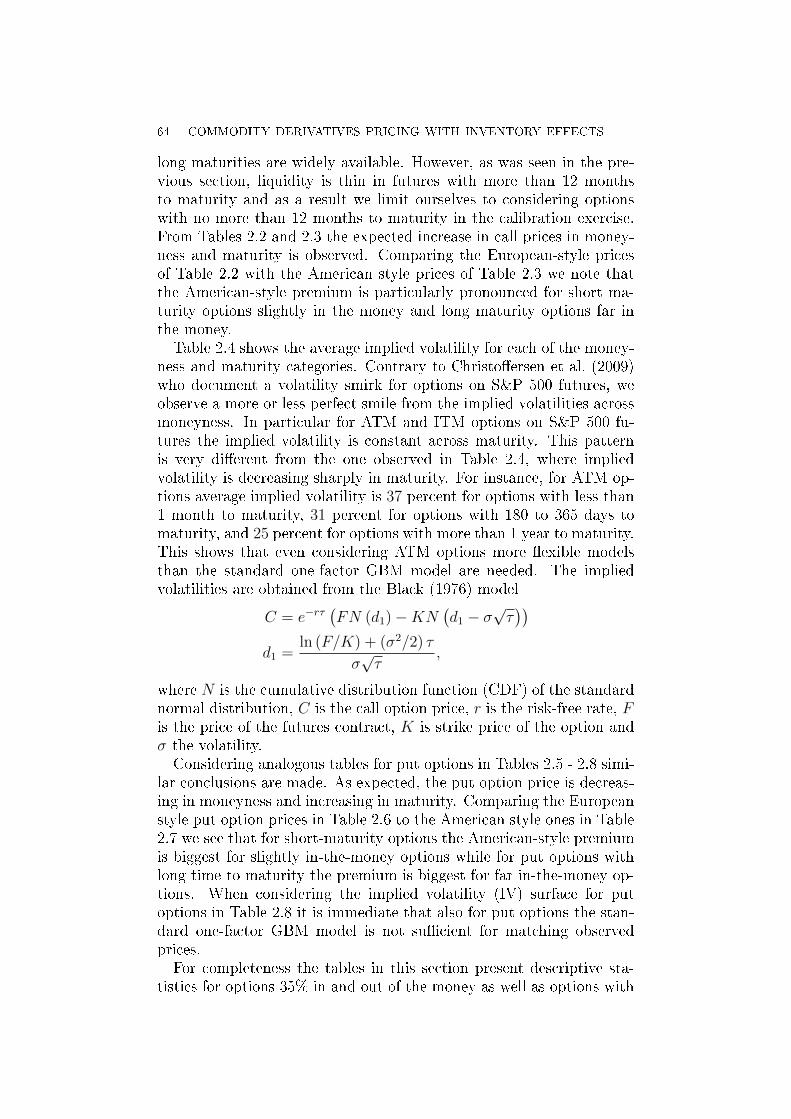
64 COMMODITY DERIVATIVES PRICING WITH INVENTORY EFFECTS
long maturities are widely available. However, as was seen in the pre-vious section, liquidity is thin in futures with more than 12 monthsto maturity and as a result we limit ourselves to considering optionswith no more than 12 months to maturity in the calibration exercise.From Tables 2.2 and 2.3 the expected increase in call prices in money-ness and maturity is observed. Comparing the European-style pricesof Table 2.2 with the American style prices of Table 2.3 we note thatthe American-style premium is particularly pronounced for short ma-turity options slightly in the money and long maturity options far inthe money.Table 2.4 shows the average implied volatility for each of the money-
ness and maturity categories. Contrary to Christoersen et al. (2009)who document a volatility smirk for options on S&P 500 futures, weobserve a more or less perfect smile from the implied volatilities acrossmoneyness. In particular for ATM and ITM options on S&P 500 fu-tures the implied volatility is constant across maturity. This patternis very dierent from the one observed in Table 2.4, where impliedvolatility is decreasing sharply in maturity. For instance, for ATM op-tions average implied volatility is 37 percent for options with less than1 month to maturity, 31 percent for options with 180 to 365 days tomaturity, and 25 percent for options with more than 1 year to maturity.This shows that even considering ATM options more exible modelsthan the standard one-factor GBM model are needed. The impliedvolatilities are obtained from the Black (1976) model
C = e−rτ(FN (d1)−KN
(d1 − σ
√τ))
d1 =ln (F/K) + (σ2/2) τ
σ√τ
,
where N is the cumulative distribution function (CDF) of the standardnormal distribution, C is the call option price, r is the risk-free rate, Fis the price of the futures contract, K is strike price of the option andσ the volatility.Considering analogous tables for put options in Tables 2.5 - 2.8 simi-
lar conclusions are made. As expected, the put option price is decreas-ing in moneyness and increasing in maturity. Comparing the Europeanstyle put option prices in Table 2.6 to the American style ones in Table2.7 we see that for short-maturity options the American-style premiumis biggest for slightly in-the-money options while for put options withlong time to maturity the premium is biggest for far in-the-money op-tions. When considering the implied volatility (IV) surface for putoptions in Table 2.8 it is immediate that also for put options the stan-dard one-factor GBM model is not sucient for matching observedprices.For completeness the tables in this section present descriptive sta-
tistics for options 35% in and out of the money as well as options with

COMMODITY DERIVATIVES PRICING WITH INVENTORY EFFECTS 65
more than 1 year to maturity. In the calibration we limit the sampleto include options 20% in and out of the money and we only includeoptions with more than 1 year to maturity if they are written on eitherthe December or June contracts.
Number of call option contracts
14 ≤ τ ≤ 30 30 < τ ≤ 90 90 < τ ≤ 180 180 < τ ≤ 360 360 < τ All
0.65 < K/F < 0.7 1,706 7,462 8,718 9,996 15,131 43,0130.7 < K/F < 0.75 3,001 13,342 14,049 13,511 19,371 63,2740.75 < K/F < 0.8 5,318 19,281 19,412 17,691 24,477 86,1790.8 < K/F < 0.85 7,923 25,237 26,112 23,227 30,001 112,5000.85 < K/F < 0.9 9,794 30,499 34,406 31,319 32,278 138,2960.9 < K/F < 0.925 5,355 16,825 19,999 19,334 16,602 78,1150.925 < K/F < 0.95 5,553 17,748 21,793 22,061 17,287 84,4420.95 < K/F < 0.975 5,720 18,494 23,105 24,558 18,009 89,8860.975 < K/F < 1 5,443 19,285 24,580 26,910 18,784 95,0021 < K/F < 1.025 4,892 18,241 23,458 25,248 17,002 88,841
1.025 < K/F < 1.05 4,425 17,099 21,559 21,648 14,550 79,2811.05 < K/F < 1.075 3,420 15,836 19,456 19,906 12,983 71,6011.075 < K/F < 1.1 2,203 14,531 17,594 17,599 11,581 63,5081.1 < K/F < 1.15 2,181 23,357 30,784 29,586 20,558 106,4651.15 < K/F < 1.2 1,025 14,753 24,766 23,976 18,591 83,1111.2 < K/F < 1.25 554 8,126 17,865 18,482 16,530 61,5571.25 < K/F < 1.3 306 4,588 11,605 14,330 14,833 45,6621.3 < K/F < 1.35 143 3,011 7,634 10,913 13,796 35,497
All 68,962 287,714 366,895 370,295 332,364 1,426,230
Table 2.1. Number of call option contracts for dierent maturitiesand strike, 1988-2011.
Average European call price
14 ≤ τ ≤ 30 30 < τ ≤ 90 90 < τ ≤ 180 180 < τ ≤ 360 360 < τ All
0.65 < K/F < 0.7 23.99 22.20 11.94 6.53 5.11 10.540.7 < K/F < 0.75 20.19 17.48 10.00 3.89 4.24 8.990.75 < K/F < 0.8 15.33 11.87 5.42 3.05 5.34 6.970.8 < K/F < 0.85 10.72 6.83 2.60 3.27 6.18 5.210.85 < K/F < 0.9 6.35 3.05 2.32 3.89 7.14 4.250.9 < K/F < 0.925 3.56 1.92 2.80 4.36 8.06 4.170.925 < K/F < 0.95 2.01 1.97 3.21 4.84 8.70 4.420.95 < K/F < 0.975 1.39 2.31 3.70 5.26 9.26 4.810.975 < K/F < 1 1.68 2.82 4.30 5.76 9.91 5.371 < K/F < 1.025 1.97 3.09 4.43 5.85 10.35 5.561.025 < K/F < 1.05 1.51 2.63 3.80 5.23 9.90 4.931.05 < K/F < 1.075 1.23 2.20 3.34 4.74 9.37 4.471.075 < K/F < 1.1 1.13 1.74 2.96 4.32 8.85 4.091.1 < K/F < 1.15 1.09 1.53 2.45 3.76 8.24 3.701.15 < K/F < 1.2 0.98 1.33 1.94 3.43 7.45 3.391.2 < K/F < 1.25 0.84 1.28 1.67 2.59 6.71 3.241.25 < K/F < 1.3 0.75 1.28 1.57 2.32 6.16 3.261.3 < K/F < 1.35 0.71 1.22 1.53 2.13 5.68 3.30
All 5.87 4.50 3.54 4.23 7.45 4.94
Table 2.2. Average European call option price for dierent maturi-ties and strike, 1988-2011. The European price is obtained by applyingthe Ju formula conversion from American-style options.

66 COMMODITY DERIVATIVES PRICING WITH INVENTORY EFFECTS
Average American call price
14≤ τ ≤30 30< τ ≤90 90< τ ≤180 180< τ ≤360 360 < τ All
0.65 < K/F < 0.7 24.73 26.26 26.39 28.04 29.97 27.940.7 < K/F < 0.75 20.31 20.59 21.14 23.45 26.19 23.020.75 < K/F < 0.8 15.58 15.88 16.98 19.18 22.79 18.750.8 < K/F < 0.85 11.44 12.02 13.25 15.12 19.51 14.900.85 < K/F < 0.9 7.95 8.79 10.12 12.07 16.56 11.620.9 < K/F < 0.925 5.72 6.77 8.25 10.06 14.69 9.580.925 < K/F < 0.95 4.47 5.59 7.08 8.94 13.59 8.410.95 < K/F < 0.975 3.37 4.58 6.12 7.79 12.38 7.340.975 < K/F < 1 2.56 3.73 5.28 6.84 11.34 6.451 < K/F < 1.025 1.99 3.12 4.49 5.98 10.55 5.651.025 < K/F < 1.05 1.51 2.63 3.80 5.25 9.93 4.941.05 < K/F < 1.075 1.23 2.20 3.34 4.74 9.38 4.471.075 < K/F < 1.1 1.13 1.84 2.96 4.32 8.87 4.101.1 < K/F < 1.15 1.09 1.53 2.45 3.77 8.27 3.711.15 < K/F < 1.2 0.98 1.33 1.94 3.13 7.46 3.401.2 < K/F < 1.25 0.84 1.29 1.67 2.59 6.72 3.251.25 < K/F < 1.3 0.75 1.28 1.57 2.32 6.16 3.261.3 < K/F < 1.35 0.71 1.22 1.53 2.14 5.69 3.30
All 6.82 6.80 7.16 8.53 14.11 9.05
Table 2.3. Average American call option price for dierent matu-rities and strike, 1988-2011.
Average call IV
14≤ τ ≤30 30< τ ≤90 90< τ ≤180 180< τ ≤360 360 < τ All
0.65 < K/F < 0.7 0.61 0.46 0.40 0.36 0.30 0.370.7 < K/F < 0.75 0.54 0.44 0.39 0.35 0.29 0.370.75 < K/F < 0.8 0.48 0.42 0.37 0.35 0.28 0.360.8 < K/F < 0.85 0.44 0.39 0.36 0.33 0.27 0.350.85 < K/F < 0.9 0.41 0.38 0.35 0.32 0.27 0.330.9 < K/F < 0.925 0.39 0.37 0.34 0.31 0.26 0.330.925 < K/F < 0.95 0.38 0.36 0.34 0.31 0.26 0.320.95 < K/F < 0.975 0.37 0.36 0.33 0.31 0.26 0.320.975 < K/F < 1 0.37 0.35 0.33 0.30 0.25 0.311 < K/F < 1.025 0.38 0.36 0.33 0.30 0.25 0.321.025 < K/F < 1.05 0.38 0.36 0.33 0.30 0.26 0.321.05 < K/F < 1.075 0.40 0.37 0.34 0.31 0.26 0.331.075 < K/F < 1.1 0.44 0.37 0.35 0.31 0.26 0.331.1 < K/F < 1.15 0.52 0.39 0.35 0.31 0.26 0.341.15 < K/F < 1.2 0.63 0.42 0.36 0.32 0.27 0.341.2 < K/F < 1.25 0.72 0.48 0.38 0.33 0.27 0.351.25 < K/F < 1.3 0.81 0.55 0.41 0.34 0.28 0.361.3 < K/F < 1.35 0.88 0.61 0.43 0.35 0.28 0.36
All 0.43 0.39 0.35 0.32 0.27 0.34
Table 2.4. Average IV for call options for dierent maturities andstrike, 1988-2011.
2.3. Inventory Data. Several inventories data are available, but asargued by Gabillon (1991) the relevant series for derivatives pricing isthe commercial inventories series. This series is updated on a weeklybasis and available from the U.S. Energy Information Administration.As mentioned earlier, it is widely documented in the literature that forcommodities in general and oil in particular inventories inuence prices
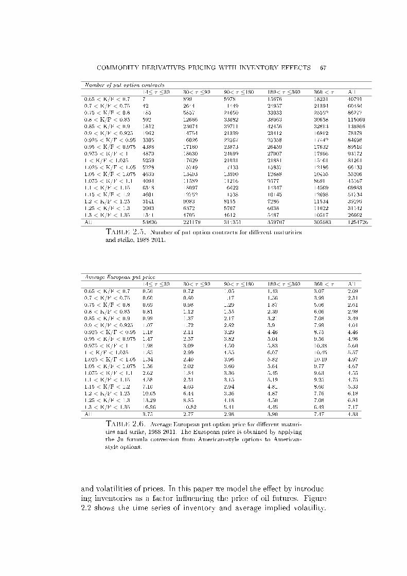
COMMODITY DERIVATIVES PRICING WITH INVENTORY EFFECTS 67
Number of put option contracts
14≤ τ ≤30 30< τ ≤90 90< τ ≤180 180< τ ≤360 360 < τ All
0.65 < K/F < 0.7 7 899 5978 15676 18231 407910.7 < K/F < 0.75 42 2644 11449 24957 21394 604860.75 < K/F < 0.8 185 5857 21650 33033 25552 862770.8 < K/F < 0.85 592 12666 33082 38063 30658 1150600.85 < K/F < 0.9 1812 23074 39711 42456 32813 1398660.9 < K/F < 0.925 1962 14754 21339 23412 16912 783790.925 < K/F < 0.95 3305 16026 22567 25358 17442 846980.95 < K/F < 0.975 4386 17160 23873 26459 17632 895100.975 < K/F < 1 4870 18630 24699 27007 17966 931721 < K/F < 1.025 5259 17629 21031 21881 15461 812611.025 < K/F < 1.05 5228 15749 17133 15837 12186 661331.05 < K/F < 1.075 4630 13493 13990 12688 10405 552061.075 < K/F < 1.1 4094 11589 11216 9577 8691 451671.1 < K/F < 1.15 6348 18097 16622 14347 14569 699831.15 < K/F < 1.2 4601 12752 11538 10145 12698 517341.2 < K/F < 1.25 3141 9083 8155 7286 11534 391991.25 < K/F < 1.3 2003 6372 5707 6038 11022 311421.3 < K/F < 1.35 1341 4705 4612 5487 10517 26662
All 53806 221179 314351 359707 305683 1254726
Table 2.5. Number of put option contracts for dierent maturitiesand strike, 1988-2011.
Average European put price
14≤ τ ≤30 30< τ ≤90 90< τ ≤180 180< τ ≤360 360 < τ All
0.65 < K/F < 0.7 0.56 0.72 1.05 1.43 3.07 2.090.7 < K/F < 0.75 0.60 0.80 1.17 1.56 3.99 2.310.75 < K/F < 0.8 0.69 0.98 1.29 1.87 5.06 2.610.8 < K/F < 0.85 0.81 1.12 1.55 2.39 6.06 2.980.85 < K/F < 0.9 0.99 1.37 2.17 3.21 7.08 3.490.9 < K/F < 0.925 1.07 1.72 2.82 3.91 7.99 4.010.925 < K/F < 0.95 1.18 2.11 3.29 4.46 8.75 4.460.95 < K/F < 0.975 1.47 2.57 3.82 5.04 9.56 4.960.975 < K/F < 1 1.98 3.09 4.50 5.83 10.38 5.601 < K/F < 1.025 1.85 2.99 4.55 6.07 10.45 5.571.025 < K/F < 1.05 1.34 2.40 3.96 5.82 10.19 4.971.05 < K/F < 1.075 1.56 2.02 3.60 5.64 9.77 4.671.075 < K/F < 1.1 2.62 1.84 3.36 5.45 9.63 4.551.1 < K/F < 1.15 4.58 2.31 3.15 5.19 9.25 4.751.15 < K/F < 1.2 7.10 4.03 2.94 4.81 8.60 5.331.2 < K/F < 1.25 10.05 6.44 3.36 4.87 7.76 6.181.25 < K/F < 1.3 13.29 8.85 4.18 4.50 7.08 6.811.3 < K/F < 1.35 16.96 10.82 5.41 4.45 6.49 7.17
All 3.75 2.77 2.98 3.90 7.47 4.33
Table 2.6. Average European put option price for dierent maturi-ties and strike, 1988-2011. The European price is obtained by applyingthe Ju formula conversion from American-style options to American-style options.
and volatilities of prices. In this paper we model the eect by introduc-ing inventories as a factor inuencing the price of oil futures. Figure2.2 shows the time series of inventory and average implied volatility.
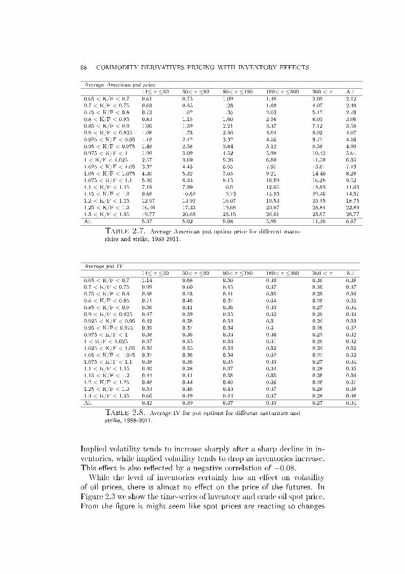
68 COMMODITY DERIVATIVES PRICING WITH INVENTORY EFFECTS
Average American put price
14≤ τ ≤30 30< τ ≤90 90< τ ≤180 180< τ ≤360 360 < τ All
0.65 < K/F < 0.7 0.61 0.75 1.09 1.46 3.09 2.120.7 < K/F < 0.75 0.63 0.85 1.23 1.68 4.07 2.400.75 < K/F < 0.8 0.73 1.02 1.35 2.03 5.12 2.700.8 < K/F < 0.85 0.83 1.15 1.60 2.56 6.09 3.060.85 < K/F < 0.9 1.00 1.39 2.21 3.37 7.12 3.560.9 < K/F < 0.925 1.08 1.73 2.86 4.04 8.02 4.070.925 < K/F < 0.95 1.18 2.12 3.32 4.56 8.77 4.500.95 < K/F < 0.975 1.48 2.58 3.84 5.12 9.58 4.990.975 < K/F < 1 1.99 3.09 4.52 5.90 10.42 5.641 < K/F < 1.025 2.57 3.69 5.26 6.80 11.50 6.351.025 < K/F < 1.05 3.32 4.43 6.05 7.97 13.01 7.191.05 < K/F < 1.075 4.30 5.32 7.05 9.21 14.40 8.281.075 < K/F < 1.1 5.40 6.33 8.15 10.59 16.28 9.521.1 < K/F < 1.15 7.19 7.99 10.01 12.65 18.93 11.631.15 < K/F < 1.2 9.88 10.62 12.73 15.93 22.46 14.971.2 < K/F < 1.25 12.97 13.92 16.07 19.53 25.55 18.751.25 < K/F < 1.3 16.46 17.33 19.68 23.07 28.84 22.891.3 < K/F < 1.35 19.77 20.63 23.15 26.61 23.07 26.77
All 5.37 5.02 5.08 5.95 11.38 6.87
Table 2.7. Average American put option price for dierent matu-rities and strike, 1988-2011.
Average put IV
14≤ τ ≤30 30< τ ≤90 90< τ ≤180 180< τ ≤360 360 < τ All
0.65 < K/F < 0.7 1.14 0.68 0.50 0.39 0.30 0.380.7 < K/F < 0.75 0.99 0.60 0.45 0.37 0.30 0.370.75 < K/F < 0.8 0.88 0.53 0.41 0.35 0.29 0.360.8 < K/F < 0.85 0.71 0.46 0.37 0.34 0.28 0.350.85 < K/F < 0.9 0.56 0.41 0.36 0.33 0.27 0.340.9 < K/F < 0.925 0.47 0.39 0.35 0.32 0.26 0.330.925 < K/F < 0.95 0.42 0.38 0.34 0.31 0.26 0.330.95 < K/F< 0.975 0.39 0.37 0.34 0.31 0.26 0.320.975 < K/F < 1 0.38 0.36 0.33 0.30 0.25 0.321 < K/F < 1.025 0.37 0.35 0.33 0.31 0.26 0.321.025 < K/F < 1.05 0.36 0.35 0.34 0.32 0.26 0.321.05 < K/F < 1.075 0.37 0.36 0.34 0.32 0.27 0.331.075 < K/F < 1.1 0.38 0.36 0.35 0.33 0.27 0.341.1 < K/F < 1.15 0.40 0.38 0.37 0.34 0.28 0.351.15 < K/F < 1.2 0.44 0.41 0.38 0.35 0.28 0.361.2 < K/F < 1.25 0.48 0.44 0.40 0.36 0.28 0.371.25 < K/F < 1.3 0.53 0.46 0.43 0.37 0.28 0.381.3 < K/F < 1.35 0.60 0.49 0.44 0.37 0.28 0.38
All 0.42 0.39 0.37 0.33 0.27 0.34
Table 2.8. Average IV for put options for dierent maturities andstrike, 1988-2011.
Implied volatility tends to increase sharply after a sharp decline in in-ventories, while implied volatility tends to drop as inventories increase.This eect is also reected by a negative correlation of −0.08.While the level of inventories certainly has an eect on volatility
of oil prices, there is almost no eect on the price of the futures. InFigure 2.3 we show the time-series of inventory and crude oil spot price.From the gure it might seem like spot prices are reacting to changes

COMMODITY DERIVATIVES PRICING WITH INVENTORY EFFECTS 69
1990 1995 2000 2005 20102
3
4x 10
5
year
Inve
ntor
y
1990 1995 2000 2005 20100
0.5
1
Ave
rage
Impl
ied
Vol
Inventory stockAverage IV
Figure 2.2. Weekly time series plots of oil inventory and averageimplied volatility. Average implied volatility is the average over optioncontracts with dierent strike and dierent maturity.
in inventories when the changes are very large, and otherwise the twoseries seem unrelated, as also indicated by a correlation coecient of−0.04.In Table 2.9 we show correlation coecients between measures of
volatility and the inventory level. For any measure of correlation andany measure of volatility correlation is negative. It is clear that em-pirical data show support for the Kaldor-Working relationship, but itis also clear that the relationship is not as strong as the one found byGeman and Nguyen (2005) for the soybean market. We are certainlynot able to write volatility as an exact inverse function of inventory.7
7Note that this analysis applies mostly to the results obtained using rankcorrelation statistics, i.e., Spearman's ρ and Kendall's τ . Since they measure(dis)agreement on the ranking one can consider rank-inversion as having an ef-fect of changing the correlation sign. At the same time, conventional Pearson'scorrelation coecient far from +/- 1 allows us to exclude the case of a perfectlinear relationship where applicable.

70 COMMODITY DERIVATIVES PRICING WITH INVENTORY EFFECTS
1985 1990 1995 2000 2005 20102.5
3
3.5
4x 10
5
year
Bar
rels
in th
ousa
nds
1985 1990 1995 2000 2005 20100
50
100
150
$ P
rice
Inventory stockOil spot
Figure 2.3. Weekly time series of oil inventory and spot oil price.
We also observe that when inventory is scarce then the Pearson cor-relation drops as low as -0.19, which indicates that when inventory isscarce volatility reacts more to changes in inventory.
Pearson Spearman Kendall
Corr(Spot,Inventory) -0.04 -0.12 -0.09Corr(RV,Inventory) -0.11 -0.24 -0.17Corr(IV,Inventory) -0.08 -0.22 -0.14Corr(IV,Inventory if scarcity(below mean)) -0.19 -0.18 -0.12
Table 2.9. The table shows Pearson, Spearman and Kendall corre-lation coecients for how inventory is correlated with the futures spotprice, futures realized volatility and option implied volatility.
3. The Models
In this section we describe the various models used in the calibration.To avoid unnecessary complexity, and without loss of generality, wedevelop all our models under the risk-neutral measure Q. The rstthing to notice is the general result that there is no drift in the futures

COMMODITY DERIVATIVES PRICING WITH INVENTORY EFFECTS 71
processes under Q. This is easily established by considering a simpleprocess for the underlying spot price
dStSt
= (r − y) dt+ σdWt,
and the standard relationship between the spot and future price
F = Se(r−y)τ ,
where r is the instantaneous risk-free rate, σ is the spot volatility and yis the convenience yield. From Ito's lemma the process for the futurescontract is given by
dFtFt
= σdWt.
We will only work with models for the futures with no drift, but wewill increase complexity of the volatility of the futures.In the following, we dene an inventory variable as
It =Invt
1, 000, 000,
where Invt is observed commercial inventories in barrels.
3.1. FV model. We consider a simple Heston two-factor (FV) modelfor futures
dFt =√VtF
βt dW
Ft , (3.1)
dVt = aV (bV − Vt) dt+ cV√VtdW
Vt , (3.2)
V0 = v0 (calibrated parameter), (3.3)[W F ,W V
]t
= ρFV t, (3.4)
where aV determines the speed of mean reversion to bV in stochas-tic volatility and β determines skewness in the distribution of futuresprices. If β = 1 the model collapses to the standard Heston model.With β 6= 1 the model also encompasses the practically very relevantstatic SABR ("stochastic alpha, beta, rho") model.8 In this paper weonly consider the simple case of β = 1. This is done for both simplicityand computational ease, however, the generalization should theoreti-cally be straightforward for β of 0, 1/2, and 1. Among those values theskewness of 1 seems to be the empirically relevant choice, see Geman(2005).
8The model is a dynamic SABR model in the most general case since ρFV iseectively only piecewise-constant (not constant) and therefore time-varying. Thisis reected in the (re)calibration methods used in the paper. In order to keep thenotation light, we do not introduce this additional temporal dependence in most ofthe formulas other than the ones used when discussing the calibration.

72 COMMODITY DERIVATIVES PRICING WITH INVENTORY EFFECTS
3.2. FI model. A simple modication of the Heston two-factor modelgives us a model utilizing the information in inventory. We still modelthe price of the future as in the Heston model, but instead of aug-menting the equation by an equation for volatility we augment it byan equation for inventory. The model is formulated as9
dFt =√ItF
βt dW
Ft , (3.5)
dIt = aI (bI − It) dt+ cI√ItdW
It , (3.6)
I0 = i0 (observed data), (3.7)[W F ,W I
]t
= ρFIt, (3.8)
where the interpretation of the coecients now apply to inventoryrather than volatility, but is otherwise the same. In practice this modelis dierent from the Heston FV model in only one aspect. Rather thancalibrating initial volatility we take initial inventory from data (hence,resulting in a more parsimonious model). This allows for much fastercalibration but also puts a severe restriction on the model. We notethat because of the restriction the model will by construction not beable to match data as well as the standard FV model (which has moredegrees of freedom). However, as will be shown in Section 5, the cali-brated model parameters are less volatile which is desirable for hedging.The FI model only performs slightly worse than the FV model in out-of-sample pricing and in some settings it is able to greatly outperformthe FV model in terms of forecasting option prices one day ahead.Using the stochastic dierential equation (SDE) approach together
with calibration oers a lot of exibility in terms of modeling. Inthis paper we only consider two-factor models, but it is not theoreti-cally much more complicated to work with three-factor models. Nat-ural models to apply from the class of three-factor models include thedouble-volatility model of Christoersen et al. (2009), a model aug-menting the SDE for futures prices with both volatility and inventoryas proposed in Appendix B, FVV and FVI models, respectively, ora model augmenting the SDE for futures prices with volatility anda latent factor only inuencing futures prices and volatility throughthe correlation structure (as proposed in Appendix B, FVL model).Semi-closed-form solutions can still be obtained for such models (seeAppendix B) and pricing is almost as fast as in two-factor models.
9Note that as more general formulation one can write dIt = aI
(bI − It
)dt +
cI
√ItdW
It , where I is a functional transformation of I. For instance, one could
focus on modeling the inverse-inventories (scarcity) levels where I = 1I . Here, we
have chosen to focus on modeling the inverse relationship via the (non-zero) instan-taneous correlations of the Wiener Processes driving the price F and inventory I.However, we have also performed an assessment of the FI model where the inven-tory data was replaced with inverse-inventory data and found no improvement inmodel performance (and even observed a deterioration).

COMMODITY DERIVATIVES PRICING WITH INVENTORY EFFECTS 73
What complicates the use of three-factor models for empirical studiesis the computational complexity when calibrating the models.
3.2.1. Specication Analysis. An empirically interesting research ques-tion is whether the proposed model ts the data for the inventory levelswell in particular, whether the distributional assumptions made arereasonable. In order to investigate it, we rst note that the continuous-time SDE (3.6) can be discretized as follows
It+∆t − It = aI(bI − It) ∆t+ cI√I tεt,
which is equivalent toIt+∆t−It√
It= aIbI∆t√
rt− aI√I t∆t+ cI εt, where εt is the error term.
This equation can be used for a linear regression. We run the regres-sion and perform a diagnostic analysis of the residuals in particular,we illustrate the Q-Q plot for the sample of data versus a theoreticaldistribution in Figure 3.1. We conclude that the model ts the dataremarkably well, leading to residuals almost completely within 95%-condence level point-wise condence envelope.
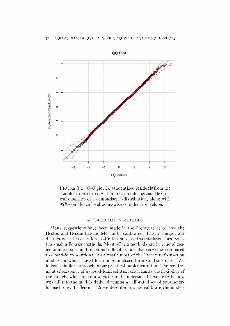
74 COMMODITY DERIVATIVES PRICING WITH INVENTORY EFFECTS
−3 −2 −1 0 1 2 3
−3
−2
−1
01
23
QQ Plot
t Quantiles
Stu
dent
ized
Res
idua
ls(f
it)
Figure 3.1. Q-Q plot for studentized residuals from thesample of data tted with a linear model against theoret-ical quantiles of a comparison t-distribution, along with95%-condence level point-wise condence envelope.
4. Calibration methods
Many suggestions have been made in the literature as to how theHeston and Heston-like models can be calibrated. The rst importantdistinction is between Monte-Carlo and closed/semi-closed form solu-tions using Fourier methods. Monte-Carlo methods are in general eas-ier to implement and much more exible, but also very slow comparedto closed-form solutions. As a result most of the literature focuses onmodels for which closed-form or semi-closed-form solutions exist. Wefollow a similar approach in our practical implementation. The require-ment of existence of a closed-form solution often limits the exibility ofthe models, which is not always desired. In Section 4.1 we describe howwe calibrate the models daily, obtaining a calibrated set of parametersfor each day. In Section 4.2 we describe how we calibrate the models

COMMODITY DERIVATIVES PRICING WITH INVENTORY EFFECTS 75
for each maturity, daily, yielding a calibrated set of parameters for eachdistinct maturity on each day. Naturally, the latter approach is muchmore exible than the former but it also requires a very liquid dataset,with several strikes traded in each maturity. Furthermore, the latterapproach is not guaranteed to (and will almost surely not) yield cali-brated parameter values that are consistent across maturities on eachday. In particular, the calibrated value of V0 could be dierent for eachmaturity on each day. It being substantially dierent across maturi-ties on each day might be a sign of model misspecication. A similarinterpretation applies to the long-run value, b (bI or bV depending onthe model). However, we also note that futures contracts with dier-ent maturity can have both dierent spot volatility and long run levelof volatility and as such these parameters are allowed to show somevariation across maturities on the same day. For both the daily andmaturity-wise calibration method we use 80% of the observations forcalibration and check the out-of-sample performance on the remaining20% of the observations.Note that, similarly to a standard approach found in numerous arti-
cles based on cross-sectional calibration, such as an implied-parameterestimation procedure in Bakshi et al. (1997), the calibration procedureis repeated for every observation date and thus allows the parameters touctuate through time. While one can also see studies relying on statis-tical estimation under the physical measure P making the assumptionof constant parameter values throughout the entire sampling period,our main focus is derivatives pricing and realistic performance assess-ment, not statistical inference. Hence, it is germane to benchmark themodels using the methodology compatible with the one used in theindustry and it is important to conform to the prevailing market con-ventions in order to provide a fair and practically relevant assessment.This is also emphasized in the sequential and adaptive calibration lit-erature, see Lindström et al. (2008).
4.1. Daily Calibration. In our daily calibrations we follow most ofthe existing literature and assume one parameter-set for all optionstraded on the given day. This set can be obtained in a number of ways.In this paper we follow Bakshi et al. (1997) and Christoersen et al.(2009) and treat the spot volatility V0 as an extra parameter to be cal-ibrated. In Christoersen et al. (2009) the spot variance is calibratedfor each day, while the rest of the parameters in the parameter-setare assumed constant each year10. We allow more exibility in ourcalibration setup and let all parameters vary each day. Let θt denotethe parameter-set at time (day) t; oit,τ the observed European optionprice at t, with maturity τ , and strikes i = 1, 2, ..., I. Further, denote
10Christoersen et al. (2009) implement this using the iterative procedure ofJing-Zhi and Wu (2004).

76 COMMODITY DERIVATIVES PRICING WITH INVENTORY EFFECTS
oit,τ
(θt
)as the model European option prices given θt. Then the ag-
gregate sum of squared pricing errors optimization problem is of theform
θt = argθt
min1
IτN
I∑
i=1
τN∑
τ=τ1
(oit,τ − oit,τ
(θt
))2
, t = 1, 2, ..., T, (4.1)
where T is the number of days in the dataset and τN is the option withthe longest time to maturity.
4.2. Daily Maturity-wise Calibration. From the descriptive statis-tics of implied volatility fromWTI options it is clear that the Samuelsoneect (volatility declines with time-to-maturity) is present in the data.It is also very likely that the options are heterogeneous in other respectsacross the maturity dimension. To allow for such heterogeneity in ourmodels we also calibrate them using what we call a daily maturity-wisecalibration approach. It is similar to the daily calibration except thatwithin each day we further calibrate a set of parameters for each matu-rity. The aggregate sum of squared pricing errors optimization problemis of the form
θt,τ = argθt,τ
min1
I
I∑
i=1
(oit,τ − oit,τ
(θt,τ
))2
, τ = τ1, τ2, ..., τN , t = 1, 2, ..., T.
(4.2)Using this calibration procedure we can analyze how the calibrated pa-rameters vary in the maturity dimension. In the Black-Scholes worldthe model performance can be assessed by considering the impliedvolatility surface. In a similar fashion this calibration procedure allowsus to assess the validity of our model by considering parameters acrossmaturity. For example, for the Heston model the calibrated value ofspot volatility V0 and long-term volatility b should not vary too muchacross maturity. In the FV model b should be constant across maturity,since the long run inventory should be independent of maturity.
5. Results
In this section we present results across the models and calibrationmethods. The all-dominating goal of the calibrations is to investigatewhich models have the best out-of-sample t. We also investigate howthe parameters of the models have changed historically, as well as thecorrelation structure between parameters and ts. In the FI models itis possible to investigate the importance of including inventory data inthe analysis. In the maturity-wise calibrations it is further possible toinvestigate the dierence in parameters as a function of maturity of theoptions. As such the dierent models and dierent calibrations allowsfor analysis of the models in various dimensions.
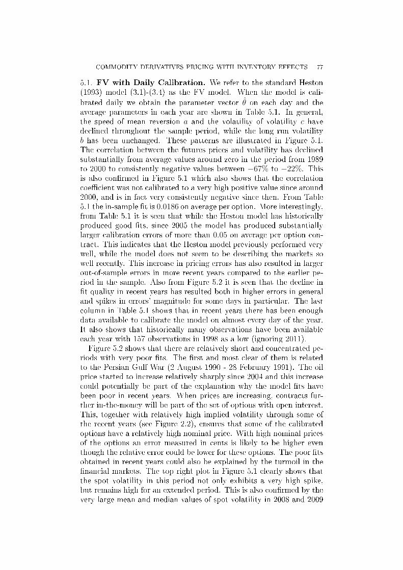
COMMODITY DERIVATIVES PRICING WITH INVENTORY EFFECTS 77
5.1. FV with Daily Calibration. We refer to the standard Heston(1993) model (3.1)-(3.4) as the FV model. When the model is cali-
brated daily we obtain the parameter vector θ on each day and theaverage parameters in each year are shown in Table 5.1. In general,the speed of mean reversion a and the volatility of volatility c havedeclined throughout the sample period, while the long run volatilityb has been unchanged. These patterns are illustrated in Figure 5.1.The correlation between the futures prices and volatility has declinedsubstantially from average values around zero in the period from 1989to 2000 to consistently negative values between −67% to −22%. Thisis also conrmed in Figure 5.1 which also shows that the correlationcoecient was not calibrated to a very high positive value since around2000, and is in fact very consistently negative since then. From Table5.1 the in-sample t is 0.0186 on average per option. More interestingly,from Table 5.1 it is seen that while the Heston model has historicallyproduced good ts, since 2005 the model has produced substantiallylarger calibration errors of more than 0.05 on average per option con-tract. This indicates that the Heston model previously performed verywell, while the model does not seem to be describing the markets sowell recently. This increase in pricing errors has also resulted in largerout-of-sample errors in more recent years compared to the earlier pe-riod in the sample. Also from Figure 5.2 it is seen that the decline int quality in recent years has resulted both in higher errors in generaland spikes in errors' magnitude for some days in particular. The lastcolumn in Table 5.1 shows that in recent years there has been enoughdata available to calibrate the model on almost every day of the year.It also shows that historically many observations have been availableeach year with 157 observations in 1998 as a low (ignoring 2011).Figure 5.2 shows that there are relatively short and concentrated pe-
riods with very poor ts. The rst and most clear of them is relatedto the Persian Gulf War (2 August 1990 - 28 February 1991). The oilprice started to increase relatively sharply since 2004 and this increasecould potentially be part of the explanation why the model ts havebeen poor in recent years. When prices are increasing, contracts fur-ther in-the-money will be part of the set of options with open interest.This, together with relatively high implied volatility through some ofthe recent years (see Figure 2.2), ensures that some of the calibratedoptions have a relatively high nominal price. With high nominal pricesof the options an error measured in cents is likely to be higher eventhough the relative error could be lower for these options. The poor tsobtained in recent years could also be explained by the turmoil in thenancial markets. The top right plot in Figure 5.1 clearly shows thatthe spot volatility in this period not only exhibits a very high spike,but remains high for an extended period. This is also conrmed by thevery large mean and median values of spot volatility in 2008 and 2009

78 COMMODITY DERIVATIVES PRICING WITH INVENTORY EFFECTS
Year a b c ρ V0 In-sample t Out-of-sample t Obs.
1989 5.1474 0.0880 0.7258 -0.2969 0.0647 0.0004 0.0005 2071990 12.9015 0.0476 0.8728 0.0479 0.2845 0.0271 0.0283 2131991 10.6445 0.0488 0.6747 0.0564 0.1295 0.0025 0.0031 2281992 9.1133 0.0342 0.6300 -0.0756 0.0604 0.0008 0.0010 2471993 31.2863 0.0471 0.8643 -0.2944 0.1943 0.0022 0.0024 2311994 11.8673 0.0299 0.4831 -0.0854 0.1589 0.0019 0.0019 2341995 7.8791 0.0140 0.3368 0.0963 0.0694 0.0019 0.0024 2401996 16.5844 0.0197 0.5427 -0.0837 0.2248 0.0059 0.0057 2091997 31.1093 0.0434 0.7238 0.0931 0.3429 0.0151 0.0197 1871998 10.5215 0.0284 0.3888 0.0716 0.2800 0.0140 0.0132 1571999 10.3661 0.0717 0.4550 -0.0793 0.3087 0.0120 0.0126 1812000 3.9926 0.0297 0.4146 -0.1344 0.1896 0.0034 0.0033 2422001 3.1533 0.0361 0.3119 -0.4575 0.2108 0.0088 0.0094 2232002 3.1871 0.0435 0.3468 -0.6159 0.2222 0.0127 0.0120 2322003 8.4717 0.0404 0.5547 -0.6723 0.2429 0.0085 0.0084 2322004 5.2114 0.0341 0.4976 -0.2224 0.1958 0.0135 0.0145 2452005 1.3102 0.0351 0.2906 -0.2828 0.1478 0.0109 0.0109 2512006 5.6137 0.0411 0.3563 -0.5210 0.1326 0.0223 0.0228 2502007 1.6672 0.0246 0.2762 -0.5325 0.1039 0.0260 0.0271 2492008 2.2240 0.0277 0.2822 -0.2286 0.3318 0.0710 0.0721 2422009 2.0372 0.0413 0.3731 -0.6611 0.3579 0.0552 0.0552 2502010 0.7158 0.0480 0.2598 -0.6052 0.1281 0.0615 0.0623 2522011 0.8471 0.0396 0.2559 -0.4941 0.1114 0.0710 0.0708 85
Mean 8.3146 0.0392 0.4741 -0.2677 0.1935 0.0186 0.0191 221
Table 5.1. Mean of the parameter values and ts for each yearusing the number of observations shown in the last column. In-samplet is the minimized value of criterion function Eq. (4.1) and out-of-sample t is the out-of-sample equivalent. The results are for the dailycalibrated FV model.
as reported in Tables 5.1 and 5.2. In fact 2009 has by far the largestmedian spot volatility of 28% which is very high for oil futures.From Table 5.2, which reports medians as opposed to the mean values
considered above, several important points can be made. The speedof mean-reversion of volatility a, long-run volatility b, and volatility ofvolatility c all have outliers and the reported medians are substantiallylower than the mean values. The correlation between futures prices andvolatility ρ on the other hand has largely similar median values as themeans. Medians of ts of the model are substantially lower than theirmeans reported above in Table 5.1. This indicates that the Hestonmodel is in general better than what was suggested by the above meanvalues. However, in recent years the median values have been just aspoor as the mean values, supporting the notion that the Heston modelhas been relatively worse in recent years.Table 5.3 shows the standard deviation of the parameter estimates
and ts. While the model t was relatively poor in recent years interms of mean and median in-sample and out-of-sample ts standarddeviations of ts are only large in 2008 and 2009, when the crisis wasat its peak. In 2010 and 2011 the standard deviation is much in linewith what can be considered normal. The same pattern is seen in thestandard deviation of spot volatility V0. Not surprisingly, the standard
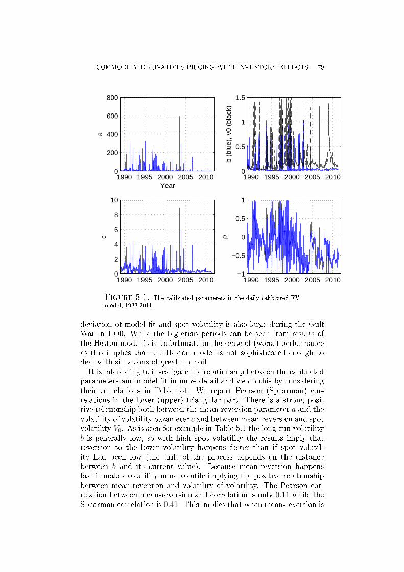
COMMODITY DERIVATIVES PRICING WITH INVENTORY EFFECTS 79
1990 1995 2000 2005 20100
200
400
600
800a
Year1990 1995 2000 2005 2010
0
0.5
1
1.5
b (b
lue)
, v0
(bla
ck)
1990 1995 2000 2005 20100
2
4
6
8
10
c
1990 1995 2000 2005 2010−1
−0.5
0
0.5
1
ρ
Figure 5.1. The calibrated parameters in the daily calibrated FVmodel, 1988-2011.
deviation of model t and spot volatility is also large during the GulfWar in 1990. While the big crisis periods can be seen from results ofthe Heston model it is unfortunate in the sense of (worse) performanceas this implies that the Heston model is not sophisticated enough todeal with situations of great turmoil.It is interesting to investigate the relationship between the calibrated
parameters and model t in more detail and we do this by consideringtheir correlations in Table 5.4. We report Pearson (Spearman) cor-relations in the lower (upper) triangular part. There is a strong posi-tive relationship both between the mean-reversion parameter a and thevolatility of volatility parameter c and between mean-reversion and spotvolatility V0. As is seen for example in Table 5.1 the long-run volatilityb is generally low, so with high spot volatility the results imply thatreversion to the lower volatility happens faster than if spot volatil-ity had been low (the drift of the process depends on the distancebetween b and its current value). Because mean-reversion happensfast it makes volatility more volatile implying the positive relationshipbetween mean-reversion and volatility of volatility. The Pearson cor-relation between mean-reversion and correlation is only 0.11 while theSpearman correlation is 0.41. This implies that when mean-reversion is

80 COMMODITY DERIVATIVES PRICING WITH INVENTORY EFFECTS
1990 1995 2000 2005 20100
0.2
0.4
0.6
0.8
1In
sam
ple
func
tion
valu
e
1990 1995 2000 2005 20100
0.2
0.4
0.6
0.8
1
Out
of s
ampl
e fu
nctio
n va
lue
Figure 5.2. In-sample and out-of-sample t in the daily calibratedFV model, 1988-2011. In-sample t is the minimized value of criterionfunction Eq. (4.1) and out-of-sample t is the out-of-sample equivalent.
large then futures and volatility are more strongly correlated, but moreso in the non-linear Spearman correlation than in the linear Pearsoncorrelation sense.It is further interesting that the long-run variance parameter b does
not seem to be correlated with the other parameters and t measuresin the linear Pearson sense, but is relatively strongly correlated with allthe remaining parameters and both t measures in the non-linear (rank-ing) Spearman sense. Not surprisingly, the correlation between the in-and out-of-sample t is almost unity implying that when the modelhas poor in-sample t it also has poor out-of-sample t. In- and out-of-sample t are strongly correlated with the parameters of the modelin terms of Spearman correlation. If volatility is high, as indicated byspot volatility and/or high long-run variance, then the model performsworse in explaining data. This could imply that the Heston model isnot the correct model for underlying volatility and that one should lookfor a richer model. However, it could also imply that the calibrationprocedure is too strict and indeed we show in Section 5.3 that when we

COMMODITY DERIVATIVES PRICING WITH INVENTORY EFFECTS 81
Year a b c ρ V0 In-sample t Out-of-sample t Obs.
1989 3.9232 0.0695 0.7099 -0.2880 0.0602 0.0002 0.0002 2071990 11.0749 0.0358 0.9108 -0.0690 0.1299 0.0007 0.0009 2131991 6.9445 0.0384 0.7377 0.0646 0.0536 0.0007 0.0007 2281992 6.7691 0.0277 0.6054 -0.0569 0.0419 0.0003 0.0005 2471993 8.1073 0.0234 0.5676 -0.2477 0.0594 0.0006 0.0006 2311994 4.8918 0.0157 0.3895 -0.1876 0.1062 0.0007 0.0008 2341995 3.0107 0.0128 0.2751 0.0707 0.0520 0.0006 0.0007 2401996 8.9506 0.0122 0.4378 -0.1530 0.1371 0.0016 0.0015 2091997 4.3124 0.0140 0.3226 0.1786 0.1114 0.0109 0.0088 1871998 7.1159 0.0118 0.4032 0.1296 0.2199 0.0029 0.0026 1571999 2.1947 0.0160 0.2568 -0.1003 0.1869 0.0041 0.0039 1812000 3.4040 0.0238 0.4117 -0.1456 0.1708 0.0018 0.0017 2422001 1.6462 0.0221 0.2603 -0.4111 0.1484 0.0028 0.0029 2232002 1.8769 0.0244 0.2871 -0.6297 0.1837 0.0035 0.0033 2322003 2.6057 0.0290 0.4696 -0.6524 0.1503 0.0048 0.0049 2322004 2.9314 0.0315 0.4537 -0.1892 0.1656 0.0073 0.0075 2452005 1.2046 0.0341 0.2756 -0.1709 0.1428 0.0071 0.0076 2512006 0.7804 0.0414 0.2351 -0.4832 0.0861 0.0139 0.0145 2502007 1.2084 0.0247 0.2361 -0.5524 0.0949 0.0209 0.0211 2492008 1.5418 0.0277 0.2694 -0.1808 0.2183 0.0537 0.0553 2422009 1.8724 0.0415 0.3882 -0.6621 0.2810 0.0424 0.0430 2502010 0.7071 0.0481 0.2548 -0.6219 0.1262 0.0577 0.0574 2522011 0.8211 0.0404 0.2549 -0.5298 0.1042 0.0707 0.0660 85
Median 2.7992 0.0274 0.3473 -0.2650 0.1293 0.0042 0.0039 232
Table 5.2. Medians of the parameter values and ts for the dailycalibrated FV model, 1988-2011, using the number of observationsshown in the last column. In-sample t is the minimized value of crite-rion function Eq. (4.1) and out-of-sample t is the out-of-sample equiv-alent. The results are for the FV model calibrated daily.
apply the maturity-wise approach to calibration we obtain much betterts and the model explains the data well both in high and low volatilityregimes. Table 5.4 further shows that if mean-reversion, volatility ofvolatility and/or correlation between futures prices and volatility arehigh then the model explains data better.
5.2. FI with Daily Calibration. For our slight modication of theFV (or Heston, 1993) model, the FI model, we present median pa-rameter values and model ts in Table 5.5. Instead of calibrating thespot volatility we take I0 as being the inventory observed from data.While this gives us one parameter less to calibrate, this simplicationcomes at a cost in terms of model t. Comparing model t in Table5.5 to the t in Table 5.1 the FI model on average produces more than4 times larger errors and this is particularly pronounced in the morerecent data. Considering I0 two likely explanations for this can be men-tioned. First, I0 in the FI model is remarkably constant compared toV0 in the FV model implying that the more volatile V0 provides a betterdescription of data. Second, comparing the level of the two series, V0
in the FV model is in general smaller than I0 in the FI model and sincethe long run level of volatility in FV and inventory in the FI modelare more or less equal, the FI model requires a stronger mean reversion

82 COMMODITY DERIVATIVES PRICING WITH INVENTORY EFFECTS
Year a b c ρ V0 In-sample t Out-of-sample t Obs.
1989 4.4140 0.0892 0.1721 0.1736 0.0258 0.0007 0.0012 2071990 14.9255 0.0847 0.3672 0.3700 0.3076 0.0877 0.0875 2131991 26.1520 0.0872 0.4640 0.2694 0.2071 0.0098 0.0151 2281992 18.0561 0.0547 0.3042 0.1245 0.1084 0.0027 0.0032 2471993 41.9794 0.1155 0.6280 0.2522 0.2570 0.0047 0.0049 2311994 27.0343 0.0919 0.4496 0.3704 0.1893 0.0038 0.0043 2341995 30.4145 0.0064 0.4305 0.2014 0.1028 0.0122 0.0150 2401996 29.2010 0.0671 0.4592 0.3580 0.2990 0.0124 0.0130 2091997 47.1391 0.1279 0.7862 0.3864 0.4073 0.0211 0.0336 1871998 17.0151 0.1171 0.2802 0.4465 0.2437 0.0396 0.0312 1571999 23.5707 0.1860 0.7245 0.2971 0.3672 0.0178 0.0207 1812000 4.8341 0.0581 0.1904 0.1745 0.0722 0.0070 0.0071 2422001 10.4572 0.0967 0.3579 0.2156 0.1604 0.0291 0.0337 2232002 8.2570 0.1078 0.3280 0.2407 0.1496 0.0308 0.0313 2322003 43.2342 0.0651 0.7123 0.2105 0.2117 0.0105 0.0104 2322004 12.5346 0.0287 0.4252 0.3481 0.1872 0.0210 0.0270 2452005 0.8448 0.0081 0.0900 0.2589 0.0238 0.0128 0.0151 2512006 21.5158 0.0100 0.5482 0.1526 0.2108 0.0268 0.0276 2502007 1.1299 0.0045 0.1037 0.2413 0.0281 0.0240 0.0298 2492008 1.4395 0.0091 0.0869 0.1489 0.3067 0.1009 0.1014 2422009 1.1065 0.0108 0.0800 0.1130 0.1975 0.0885 0.0848 2502010 0.1414 0.0050 0.0291 0.0648 0.0200 0.0258 0.0288 2522011 0.2206 0.0054 0.0404 0.1266 0.0200 0.0319 0.0333 85
Mean 16.6629 0.0599 0.3490 0.2371 0.1760 0.0270 0.0287 221
Table 5.3. Standard deviations of the parameter values and ts forthe daily calibrated FV model, 1988-2011, using the number of obser-vations shown in the last column. In-sample t is the minimized valueof criterion function Eq. (4.1) and out-of-sample t is the out-of-sampleequivalent. The last row shows the mean in the full sample period. Theresults are for the FV model calibrated daily.
a b c ρ V0 In-sample t Out-of-sample ta 1.0000 -0.2698 0.8003 0.4062 0.1370 -0.4994 -0.4904b -0.0373 1.0000 0.2417 -0.2638 -0.0736 0.2689 0.2783c 0.8694 -0.0417 1.0000 0.2193 0.0874 -0.3744 -0.3617ρ 0.1124 -0.0087 0.1150 1.0000 -0.1615 -0.3985 -0.3990v0 0.6053 -0.0644 0.5449 0.0398 1.0000 0.4799 0.4677In sample t -0.0072 0.1732 -0.0218 -0.1408 0.1892 1.0000 0.9455Out of sample t 0.0004 0.1638 -0.0151 -0.1435 0.1901 0.9556 1.0000
Table 5.4. Pearson correlations between the parameters of themodel as well as in- and out-of-sample ts are in the lower triangu-lar part and Spearman correlations are in the upper triangular part.In-sample t is the minimized value of criterion function Eq. (4.1) andout-of-sample t is the out-of-sample equivalent. The results are for theFV model calibrated daily.
parameter, which in turn also implies a larger volatility of volatilityparameter. This indicates that the restriction put on I0 is severe andmight not be desirable. Interestingly, both models produce largely sim-ilar correlation parameters. Also, the optimization algorithm involvedwith the calibration of the FI model converges to an interior solutionmore often than the FV model, which is particularly pronounced in1996-1999.

COMMODITY DERIVATIVES PRICING WITH INVENTORY EFFECTS 83
Year a b c ρ I0 In-sample t Out-of-sample t Obs.
1989 378.3763 0.0582 5.9055 -0.6922 0.3382 0.0009 0.0008 1701990 136.7611 0.0864 2.1597 -0.0937 0.3664 0.0505 0.0524 2011991 232.8515 0.0392 3.5857 0.1026 0.3450 0.0061 0.0059 2271992 441.8741 0.0301 4.4650 -0.2497 0.3366 0.0012 0.0014 2461993 210.6376 0.0228 2.2198 -0.5951 0.3409 0.0018 0.0024 2231994 40.4327 0.0300 1.4962 -0.0562 0.3344 0.0037 0.0042 2501995 62.5868 0.0193 1.1418 0.1763 0.3189 0.0040 0.0053 2401996 27.3183 0.0156 0.3359 0.0598 0.3045 0.0083 0.0075 2421997 26.5049 0.0223 1.0023 0.1131 0.3098 0.0170 0.0208 2361998 13.2298 0.0126 0.4674 0.1549 0.3334 0.0115 0.0117 1961999 9.7787 0.0373 0.6524 0.0073 0.3223 0.0139 0.0159 2432000 11.2853 0.0407 0.8557 -0.1316 0.2920 0.0095 0.0095 2472001 14.1320 0.0496 1.1101 -0.2895 0.3046 0.0211 0.0219 2242002 7.6185 0.0493 0.8310 -0.4439 0.3066 0.0212 0.0220 2382003 14.2638 0.0490 1.1521 -0.6559 0.2810 0.0233 0.0242 2312004 11.5694 0.0458 0.9583 -0.2296 0.2886 0.0325 0.0337 2442005 12.0088 0.0631 0.7992 -0.3830 0.3153 0.1233 0.1231 2512006 40.4466 0.0567 2.0305 -0.5059 0.3347 0.1102 0.1113 2502007 20.7905 0.0383 1.2003 -0.4821 0.3284 0.1727 0.1734 2462008 8.7981 0.0438 0.6865 -0.2495 0.3043 0.3365 0.3355 1982009 3.1734 0.0520 0.5392 -0.5641 0.3484 0.2347 0.2347 2292010 16.1174 0.0703 1.4491 -0.7086 0.3532 0.4371 0.4415 2502011 20.5523 0.0570 1.5020 -0.4870 0.3495 0.5147 0.5083 83
Mean 74.2761 0.0424 1.5429 -0.2621 0.3230 0.0822 0.0830 225
Table 5.5. Mean of the parameter values and ts for the dailycalibrated FI model, 1988-2011, using the number of observations shownin the last column. In-sample t is the minimized value of criterionfunction Eq. (4.1) and out-of-sample t is the out-of-sample equivalent.
In Figure 5.3 we show time series of the parameters in the model.From the top left plot it is immediate that as for the FV model themean-reversion parameter is much larger and much more volatile in theearly part of the sample period and much more stable on a lower levelin more recent data. In the FI model this is even more pronounced.In the top-right section of the plot we can see that inventory I0 is ona much higher level than the parameter for long-run inventory b. Thissuggests that the interpretation of the latent equation in the Heston(1993) model as being inventory rather than volatility might not betrue. On the other hand it is remarkable how stable the parameterestimate of long run inventory is compared to inventory. This seemsmuch more plausible than the erratic behavior thereof observed in theFV model. This stability is also desirable for forecasting and hedgingas will be apparent later. Compared to the FV model the volatility ofinventory is much more volatile early in the sample, while it behavesmuch more similarly in the recent data. As noted above correlationbetween futures prices and inventory seems to behave similarly in thetwo models.Similarly to the FV model, the FI model produces relatively large
pricing errors during the Gulf War and in particular during the nancialcrisis (see Figure 5.4). Further, since the nancial crisis the FI model

84 COMMODITY DERIVATIVES PRICING WITH INVENTORY EFFECTS
1990 1995 2000 2005 20100
200
400
600
800
1000a
Year1990 1995 2000 2005 2010
0
0.2
0.4
0.6
0.8
b (b
lue)
, I0
(bla
ck)
1990 1995 2000 2005 20100
5
10
15
20
c
1990 1995 2000 2005 2010−1
−0.5
0
0.5
1
ρ
Figure 5.3. Time series of the calibrated parameters (a, b, c, I0,and ρ) in the daily calibrated FI model.
has performed substantially and consistently worse than the FV modelin terms of both in- and out-of-sample t. However, the mis-pricingin the FI model seems to go up sharply already in 2005 (in contrastwith the FV model, Figure 5.2) and therefore the worse performanceof the FI model does not seem to be related solely to the nancialcrisis. Rather, it was around 2005 that the oil prices started to increasesharply, and maybe this (possibly with associated rise in volatility)presents a possible explanation, since the inventory data does not seemto be the driver of the increase.When considering the medians in Table 5.6 rather than means it
is immediate that the median of the mean-reversion parameter a andvolatility of volatility c in the full sample are much lower than themean. When considering median ts it is worth noting that the FImodel "only" produces about three times larger errors than the FVmodel, while means were about 4-5 times higher. Again the reason forthis lies in the fact that the FI model exhibits substantial mis-pricingonly in recent years and this mis-pricing has a larger impact on meants as compared to median ts.

COMMODITY DERIVATIVES PRICING WITH INVENTORY EFFECTS 85
1990 1995 2000 2005 20100
0.2
0.4
0.6
0.8
1In
sam
ple
func
tion
valu
e
1990 1995 2000 2005 20100
0.2
0.4
0.6
0.8
1
Out
of s
ampl
e fu
nctio
n va
lue
Figure 5.4. The t in the daily calibrated FI model. In-sample tis the minimized value of criterion function Eq. (4.1) and out-of-samplet is the out-of-sample equivalent.
The standard deviations reported in Table 5.7 conrm what was alsonoted from Figure 5.3. The mean-reversion parameter and volatilityof volatility parameter are much less stable in the FI than in the FVmodel. Contrary to this, the long-run level of inventory is much morestable than the long-run level of variance. It is tempting to concludethat this implies that the FV model is able to identify mean reversionand volatility of volatility with more certainty than the FI model whilethe reverse holds for the long-run value of either volatility or inventory.However, since the observed inventory level is almost constant and thelong run value of inventory is much lower than this value, interpretingb as the long-run value of inventory does not seem correct.Considering the correlation matrix in Table 5.8 we focus on the dif-
ferences between results for the FI and the FV model. The relationshipbetween volatility of inventory (volatility) and correlation between fu-tures prices and inventory (volatility) in the FI (FV) model has changedsign as compared to the FV model. The most signicant dierence be-tween the correlation matrix in the FI and that in the FV model is that
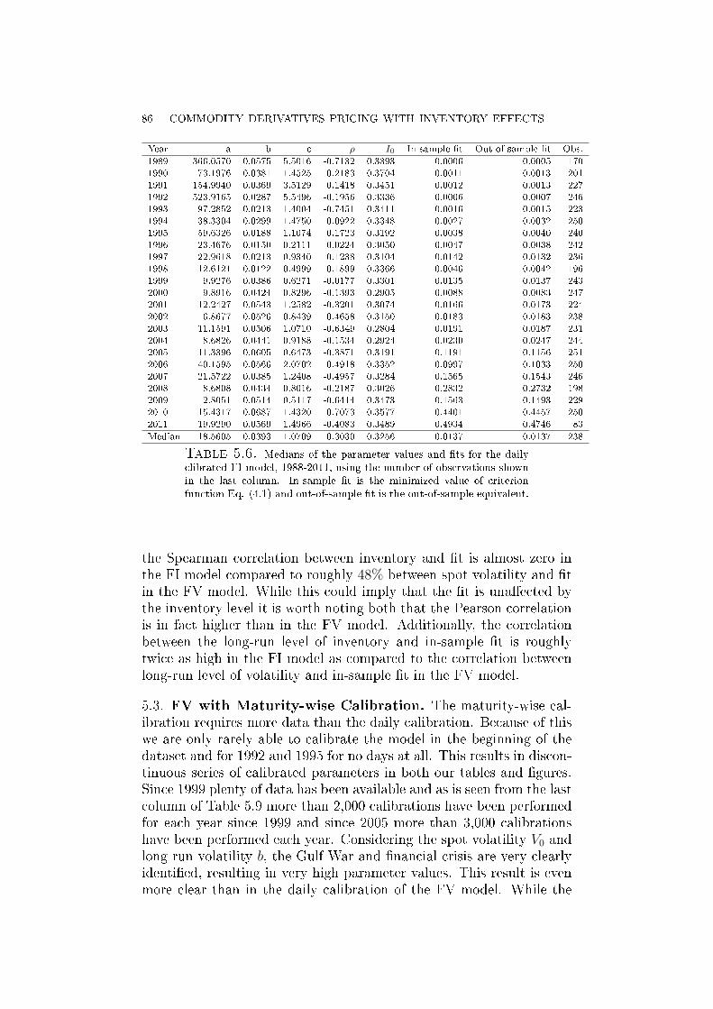
86 COMMODITY DERIVATIVES PRICING WITH INVENTORY EFFECTS
Year a b c ρ I0 In-sample t Out-of-sample t Obs.
1989 366.0570 0.0575 5.5016 -0.7132 0.3393 0.0006 0.0005 1701990 73.1976 0.0381 1.4525 -0.2183 0.3704 0.0011 0.0013 2011991 154.9940 0.0369 3.5129 0.1418 0.3451 0.0012 0.0013 2271992 523.9165 0.0287 5.5496 -0.1956 0.3336 0.0006 0.0007 2461993 97.2852 0.0213 1.4004 -0.7451 0.3411 0.0016 0.0015 2231994 38.3304 0.0299 1.4750 -0.0922 0.3348 0.0027 0.0032 2501995 59.6326 0.0188 1.1074 0.1723 0.3192 0.0038 0.0040 2401996 23.4676 0.0150 0.2111 0.0224 0.3050 0.0047 0.0038 2421997 22.9618 0.0213 0.9340 0.1238 0.3104 0.0142 0.0132 2361998 12.6121 0.0122 0.4999 0.1899 0.3366 0.0046 0.0042 1961999 9.9276 0.0386 0.6271 -0.0177 0.3301 0.0135 0.0137 2432000 9.8916 0.0424 0.8296 -0.1393 0.2905 0.0088 0.0083 2472001 12.2427 0.0543 1.2582 -0.3201 0.3074 0.0166 0.0173 2242002 6.8677 0.0526 0.8439 -0.4658 0.3150 0.0183 0.0183 2382003 11.1591 0.0506 1.0710 -0.6349 0.2804 0.0191 0.0187 2312004 8.6826 0.0441 0.9188 -0.1534 0.2924 0.0230 0.0247 2442005 11.3396 0.0605 0.6473 -0.3871 0.3191 0.1191 0.1156 2512006 40.1595 0.0566 2.0702 -0.4918 0.3352 0.0997 0.1033 2502007 21.5722 0.0385 1.2408 -0.4957 0.3284 0.1565 0.1543 2462008 8.6808 0.0434 0.8016 -0.2187 0.3026 0.2832 0.2732 1982009 2.8051 0.0514 0.5117 -0.6414 0.3473 0.1563 0.1493 2292010 15.4317 0.0687 1.4320 -0.7073 0.3577 0.4401 0.4457 2502011 19.9290 0.0569 1.4966 -0.4083 0.3489 0.4934 0.4746 83
Median 18.5605 0.0393 1.0709 -0.3030 0.3256 0.0137 0.0137 238
Table 5.6. Medians of the parameter values and ts for the dailyclibrated FI model, 1988-2011, using the number of observations shownin the last column. In-sample t is the minimized value of criterionfunction Eq. (4.1) and out-of-sample t is the out-of-sample equivalent.
the Spearman correlation between inventory and t is almost zero inthe FI model compared to roughly 48% between spot volatility and tin the FV model. While this could imply that the t is unaected bythe inventory level it is worth noting both that the Pearson correlationis in fact higher than in the FV model. Additionally, the correlationbetween the long-run level of inventory and in-sample t is roughlytwice as high in the FI model as compared to the correlation betweenlong-run level of volatility and in-sample t in the FV model.
5.3. FV with Maturity-wise Calibration. The maturity-wise cal-ibration requires more data than the daily calibration. Because of thiswe are only rarely able to calibrate the model in the beginning of thedataset and for 1992 and 1995 for no days at all. This results in discon-tinuous series of calibrated parameters in both our tables and gures.Since 1999 plenty of data has been available and as is seen from the lastcolumn of Table 5.9 more than 2,000 calibrations have been performedfor each year since 1999 and since 2005 more than 3,000 calibrationshave been performed each year. Considering the spot volatility V0 andlong-run volatility b, the Gulf War and nancial crisis are very clearlyidentied, resulting in very high parameter values. This result is evenmore clear than in the daily calibration of the FV model. While the

COMMODITY DERIVATIVES PRICING WITH INVENTORY EFFECTS 87
Year a b c ρ I0 In-sample t Out-of-sample t Obs.
1989 235.5709 0.0184 1.7810 0.2910 0.0075 0.0012 0.0011 1701990 205.5189 0.1322 1.8910 0.5213 0.0166 0.1252 0.1282 2011991 208.3927 0.0130 1.9947 0.4349 0.0074 0.0245 0.0234 2271992 421.0125 0.0054 2.0000 0.4039 0.0097 0.0028 0.0035 2461993 344.3255 0.0063 1.9529 0.3657 0.0106 0.0014 0.0024 2231994 13.9851 0.0046 0.3105 0.4450 0.0055 0.0026 0.0032 2501995 15.2735 0.0027 0.3457 0.3696 0.0114 0.0017 0.0043 2401996 14.4331 0.0040 0.2981 0.2965 0.0056 0.0091 0.0089 2421997 13.9402 0.0060 0.3626 0.3127 0.0099 0.0129 0.0227 2361998 4.6193 0.0051 0.2082 0.4055 0.0114 0.0486 0.0416 1961999 5.5878 0.0182 0.3382 0.2443 0.0157 0.0072 0.0125 2432000 5.7438 0.0094 0.2980 0.1629 0.0073 0.0058 0.0060 2472001 10.1553 0.0225 0.5908 0.2644 0.0129 0.0142 0.0154 2242002 3.8919 0.0167 0.3291 0.1905 0.0164 0.0168 0.0260 2382003 10.3236 0.0165 0.5704 0.1230 0.0065 0.0228 0.0232 2312004 7.3229 0.0111 0.2867 0.3409 0.0120 0.0236 0.0287 2442005 5.2591 0.0132 0.4810 0.1698 0.0119 0.0513 0.0527 2512006 16.6361 0.0113 0.5660 0.1013 0.0085 0.0468 0.0503 2502007 7.8940 0.0044 0.3361 0.2194 0.0147 0.0698 0.0770 2462008 6.6220 0.0122 0.4627 0.2208 0.0106 0.1931 0.1987 1982009 1.4713 0.0202 0.2444 0.3120 0.0126 0.1814 0.1811 2292010 6.9822 0.0065 0.2874 0.0954 0.0114 0.0666 0.0716 2502011 7.5125 0.0028 0.3029 0.3015 0.0091 0.1182 0.1283 83
Mean 66.8833 0.0153 0.6931 0.2828 0.0107 0.0420 0.0447 225
Table 5.7. Standard deviations of the parameter values and ts forthe FI model calibrated daily, 1988-2011, using the number of observa-tions shown in the last column. In-sample t is the minimized value ofcriterion function Eq. (4.1) and out-of-sample t is the out-of-sampleequivalent.
a b c ρ I0 In-sample t Out-of-sample ta 1.0000 -0.1698 0.7490 -0.0100 0.3651 -0.5954 -0.5774b -0.0678 1.0000 0.3318 -0.4108 0.0627 0.5076 0.5083c 0.8542 0.0655 1.0000 -0.2302 0.3575 -0.2642 -0.2458ρ -0.0609 -0.1367 -0.1536 1.0000 -0.1584 -0.2455 -0.2505I0 0.2418 0.0918 0.3168 -0.0795 1.0000 -0.0897 -0.0748In sample t -0.1845 0.3406 -0.1555 -0.2449 0.2481 1.0000 0.9710Out of sample t -0.1844 0.3423 -0.1548 -0.2456 0.2484 0.9907 1.0000
Table 5.8. Pearson correlations between the parameters of themodel as well as the in- and out-of-sample ts in the lower triangularpart and Spearman correlations in the upper triangular part. In-samplet is the minimized value of criterion function Eq. (4.1) and out-of-sample t is the out-of-sample equivalent. The results are for the FImodel calibrated daily.
long-run volatility was substantially below spot volatility on averagein the daily calibration this is not so in the maturity-wise calibrationwhere these values seem of the same level in general. This makes theinterpretation of the latent factor in the Heston (1993) model as be-ing volatility more plausible, and the model more credible. While theresults in the daily calibration implied that the mean-reversion param-eter and the volatility of volatility parameter decreased throughout thesample period this is not replicated in the maturity-wise calibration.

88 COMMODITY DERIVATIVES PRICING WITH INVENTORY EFFECTS
Mean-reversion and volatility of volatility seem either constant or per-haps even increasing throughout the sample period. However, one hasto be somewhat cautious in the interpretation of mean-reversion andlong-run volatility in maturity-wise calibration since the options arecalibrated for one maturity at a time, which eliminates one dimensionfrom the model.In practice investors care about how the model ts the data and in
particular about how it performs in terms of out-of-sample t. FromTable 5.9 it is seen that the maturity-wise calibration improves sub-stantially over the daily calibration method in terms of both in- andout-of-sample t. The average in-sample t in the maturity-wise cal-ibration is 0.0054 compared to 0.0186 in the daily calibration. Thatis, the daily calibration results in more than three times higher errors.This is particularly impressive since the bulk of observations in thematurity-wise calibration is in the end of the sample, where the He-ston model has the worst performance. It is also worth noting thateven though the maturity-wise calibration, in general, also producesthe largest errors in the last years of the sample, this feature is muchless pronounced than was the case in the FV model with daily cali-bration. A natural explanation for this is that recently more contractswith long maturities are trading, which increases the need for a moreexible model and therefore favors the maturity-wise calibration rela-tively more in this period. The out-of-sample MSE is also improvedfrom 0.0191 in the daily calibration to 0.0071 in the maturity-wise cal-ibration, an improvement of 63%.When the medians in Table 5.10 are considered instead of means the
alignment in the level of spot volatility and long-run volatility is main-tained and the long-run volatility is still slightly higher than the spotvolatility. In medians the convergence rate a and volatility of volatilityc are now either stable or slightly decreasing through the sample period.This is dierent from the conclusion drawn from considering the meansbut more in line with what has been observed in the daily calibrationof the FV model. More importantly, the maturity-wise calibration isstill strongly outperforming the daily calibration both in terms of in-sample MSE and out-of-sample MSE. This improvement amounts toroughly 60% lower magnitude of errors. The strong performance ofthe maturity-wise FV model relative to the daily FV model is evenmore pronounced in recent years. Thus the maturity-wise FV modelproduces average MSE from 2007 to 2011 of 0.004 while the daily FVmodel produces MSE of 0.049 or a reduction of the MSE of more than90%.From Table 5.11 it is seen that all parameters of the model except
spot volatility have a higher standard deviation in the maturity-wisecalibrated FV model than in the daily calibrated FV model. This isnot surprising since each maturity on each day is in principle a contract

COMMODITY DERIVATIVES PRICING WITH INVENTORY EFFECTS 89
Year a b c ρ v0 In-sample t Out-of-sample t Obs.
1990 10.8314 0.5352 2.4666 0.3155 0.4520 0.0313 0.0414 4311991 15.4419 0.3441 1.7193 0.2888 0.2613 0.0023 0.0030 3031993 7.6720 0.2040 0.8425 -0.3849 0.0877 0.0003 0.0005 741994 8.8503 0.2052 0.6785 0.0045 0.0971 0.0003 0.0006 1521996 11.4053 0.2333 0.9619 -0.0082 0.1203 0.0028 0.0065 7171997 10.2040 0.1474 0.6013 0.1476 0.1266 0.0026 0.0083 4951998 8.3572 0.1365 0.5893 0.1526 0.1538 0.0020 0.0027 10251999 8.7915 0.1544 0.6685 -0.0898 0.1585 0.0021 0.0023 20372000 12.7659 0.1375 1.0070 -0.1689 0.1671 0.0017 0.0020 25732001 11.5890 0.1763 1.1435 -0.3288 0.1849 0.0023 0.0041 23512002 7.3007 0.2061 0.9860 -0.4931 0.1578 0.0028 0.0089 24852003 9.8856 0.2472 1.2063 -0.5210 0.1160 0.0027 0.0036 22772004 20.6173 0.2121 1.2062 -0.1804 0.1439 0.0027 0.0033 27092005 13.7142 0.1373 1.0645 -0.1761 0.1297 0.0032 0.0040 36122006 22.5366 0.1292 1.0425 -0.2876 0.0850 0.0043 0.0055 37062007 30.5766 0.1195 1.1565 -0.3607 0.1115 0.0067 0.0074 35732008 54.1089 0.2397 1.8441 -0.1405 0.2595 0.0122 0.0173 37262009 10.4117 0.2924 1.5628 -0.4961 0.2389 0.0077 0.0089 36592010 9.5330 0.1765 1.1787 -0.4991 0.0850 0.0069 0.0076 38482011 36.3341 0.1789 1.2463 -0.2754 0.0966 0.0118 0.0131 1253
Mean 18.8212 0.1893 1.1943 -0.2796 0.1538 0.0054 0.0071 2050
Table 5.9. The mean of the parameter values and ts for each yearusing the number of observations shown in the last column. In-sample tis the minimized value of criterion function Eq. (4.2) and out-of-samplet is the out-of-sample equivalent. The last row shows the mean in thefull sample period. The results are for the FV model calibrated for eachmaturity on each daily.
Year a b c ρ v0 In-sample t Out-of-sample t Obs.
1990 6.2494 0.4404 2.3284 0.3085 0.3882 0.0013 0.0016 4311991 4.2678 0.2021 1.1704 0.2294 0.1257 0.0005 0.0005 3031993 5.8979 0.1191 0.4662 -0.3585 0.0876 0.0002 0.0003 741994 5.3089 0.1075 0.5161 0.0990 0.0888 0.0002 0.0002 1521996 4.3281 0.1183 0.8659 0.0998 0.0822 0.0003 0.0003 7171997 6.7790 0.0582 0.4139 0.0992 0.1025 0.0001 0.0001 4951998 4.3707 0.0904 0.4241 0.1101 0.1398 0.0001 0.0002 10251999 3.7365 0.1044 0.4138 -0.0624 0.1337 0.0002 0.0003 20372000 6.8550 0.0884 0.9230 -0.1226 0.1393 0.0004 0.0004 25732001 5.2409 0.1307 1.0065 -0.2782 0.1346 0.0006 0.0006 23512002 3.8265 0.1378 0.8443 -0.4463 0.1442 0.0004 0.0005 24852003 5.0761 0.1323 1.0150 -0.5134 0.0837 0.0006 0.0006 22772004 3.9077 0.1322 0.9704 -0.0914 0.0882 0.0007 0.0007 27092005 5.0268 0.1204 0.9041 -0.1163 0.0981 0.0006 0.0006 36122006 2.7680 0.0933 0.7248 -0.2309 0.0537 0.0011 0.0012 37062007 3.8751 0.0842 0.8033 -0.3255 0.0539 0.0024 0.0026 35732008 3.3370 0.1744 1.1290 -0.0790 0.1233 0.0060 0.0062 37262009 3.4065 0.2269 1.2402 -0.4539 0.1479 0.0033 0.0034 36592010 3.4187 0.1348 0.9857 -0.4837 0.0667 0.0034 0.0034 38482011 2.0433 0.1198 0.7996 -0.3622 0.0537 0.0051 0.0056 1253
Median 4.1453 0.1230 0.9070 -0.2692 0.0955 0.0011 0.0011 2314
Table 5.10. The median of the parameter values and ts for thematurity-wise calibrated FV model, 1988-2011, using the number ofobservations shown in the last column. In-sample t is the minimizedvalue of criterion function Eq. (4.2) and out-of-sample t is the out-of-sample equivalent.

90 COMMODITY DERIVATIVES PRICING WITH INVENTORY EFFECTS
in itself with its own set of parameters which could be, and indeed is,dierent from the contracts with other maturities on the same day. Inthe daily calibration one nds parameters for the same type of contracteach day. This contract is a weighted average of all maturities oneach day, but is not likely to vary too much from day to day andthe calibrated parameters will therefore have lower standard deviation.This type of argument can also be applied to the standard deviation ofMSE. In that context it is somewhat surprising that while the standarddeviation of in-sample MSE is lower for the maturity-wise calibratedFV model than for the daily calibrated FV model it is higher for out-of-sample MSE. We believe this result is present mainly due to theMSE being much higher out-of-sample than in-sample in 1997, 2002and 2008 see Figures 5.4 and 5.6.
Year a b c ρ v0 In-sample t Out-of-sample t Obs.
1990 13.1208 0.3560 1.6384 0.3229 0.3299 0.1125 0.1600 4311991 28.3876 0.3091 1.8589 0.3002 0.3451 0.0133 0.0180 3031993 7.1529 0.2278 0.7068 0.2926 0.0519 0.0002 0.0005 741994 13.7997 0.2497 0.5260 0.4139 0.0611 0.0008 0.0026 1521996 23.2164 0.2559 0.6983 0.3833 0.1957 0.0177 0.0585 7171997 18.5136 0.2061 0.4756 0.2608 0.1667 0.0097 0.1017 4951998 80.6161 0.1591 0.6125 0.2893 0.1000 0.0240 0.0279 10251999 68.1876 0.1688 0.7504 0.3103 0.1443 0.0117 0.0149 20372000 38.2668 0.1578 0.8085 0.2872 0.1566 0.0067 0.0211 25732001 40.9422 0.1622 0.8921 0.2517 0.1701 0.0136 0.0519 23512002 22.2400 0.1913 0.7675 0.2645 0.1227 0.0151 0.1396 24852003 40.0187 0.2596 0.9062 0.2778 0.1319 0.0299 0.0499 22772004 131.2668 0.2238 1.3877 0.3619 0.2112 0.0185 0.0228 27092005 75.4589 0.1036 1.1805 0.2351 0.1511 0.0089 0.0123 36122006 148.8299 0.1414 1.4515 0.2524 0.1502 0.0144 0.0161 37062007 199.4782 0.1469 1.5911 0.2811 0.2063 0.0326 0.0431 35732008 292.3869 0.2254 2.5837 0.2418 0.3195 0.0184 0.1078 37262009 20.1198 0.2110 1.0385 0.1970 0.2473 0.0142 0.0161 36592010 21.6243 0.1438 0.7854 0.1861 0.0947 0.0101 0.0101 38482011 241.6098 0.1960 2.2907 0.3002 0.1762 0.0150 0.0181 1253
Mean 98.6876 0.1802 1.2400 0.2622 0.1800 0.0172 0.0416 2050
Table 5.11. Standard deviations of the parameter values and tsfor the maturity-wise calibrated FV model, 1988-2011, using the numberof observations shown in the last column. In-sample t is the minimizedvalue of criterion function Eq. (4.2) and out-of-sample t is the out-of-sample equivalent.
Figure 5.5 shows the parameter averages across maturities for eachday through the sample period. Since the maturity-wise model doesnot have enough data to be calibrated often enough in the early sampleperiod it is not clear whether it is able to identify the impact of theGulf War on the oil prices but the nancial crisis seems to be identiedclearly in terms of higher volatility of volatility and high spot volatility.All parameters of the model seem relatively volatile, which is similar towhat was obtained in the daily calibration. The correlation coecientalso shows the same pattern as in the daily calibration with declines

COMMODITY DERIVATIVES PRICING WITH INVENTORY EFFECTS 91
between 1995 and 2005, followed by a sharp increase and again a periodwith declines until the end of 2010.
1990 1995 2000 2005 20100
200
400
600
800
a
1990 1995 2000 2005 20100
0.5
1
1.5
b (b
lue)
, v0
(bla
ck)
1990 1995 2000 2005 20100
5
10
15
c
1990 1995 2000 2005 2010−1
−0.5
0
0.5
1ρ
Figure 5.5. The average of the calibrated parameters (a, b, c, v0,ρ) across maturity in the maturity-wise calibrated FV model.
When considering the in- and out-of-sample MSE in Figure 5.6 thematurity-wise calibration approach generally produces substantiallysmaller average MSE all through the sample period. Even the largespikes are mostly substantially lower than the spikes observed in thedaily calibration. It is also noted that the calibration methods largelyagree on the periods in which poor ts are obtained and that the tis generally worse in recent years. Finally, as in the daily calibrationthere is a relationship between in- and out-of-sample MSE, but it is notas clear-cut as in the daily calibration and will be investigated furtherbelow.Tables 5.12 - 5.14 contain the mean, median and standard deviations,
respectively, of the calibration results across maturity of the optioncontracts. These tables show several interesting results. First, theSamuelson eect is clearly observed both in the long-run volatility band the spot volatility V0, which both show a clear declining pattern inmaturity. This is in accordance with the results for implied volatility
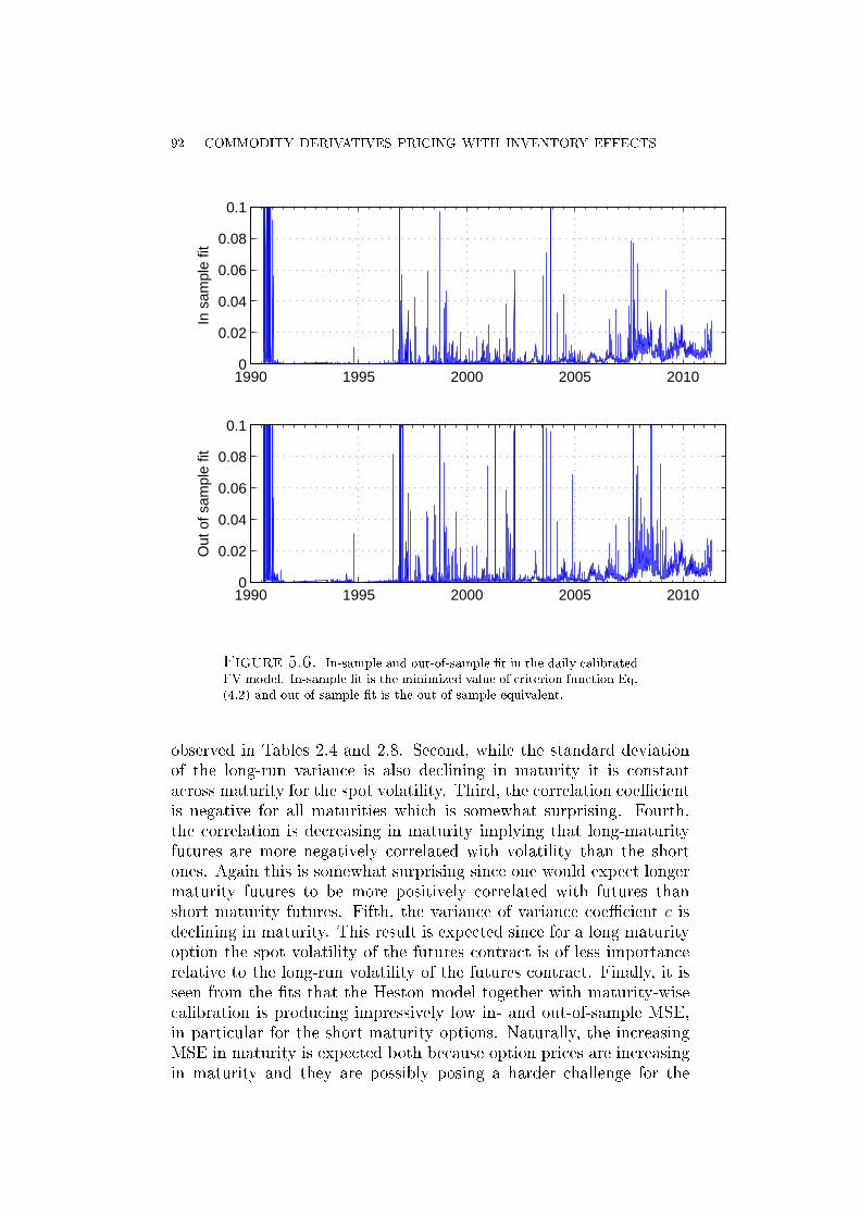
92 COMMODITY DERIVATIVES PRICING WITH INVENTORY EFFECTS
1990 1995 2000 2005 20100
0.02
0.04
0.06
0.08
0.1In
sam
ple
fit
1990 1995 2000 2005 20100
0.02
0.04
0.06
0.08
0.1
Out
of s
ampl
e fit
Figure 5.6. In-sample and out-of-sample t in the daily calibratedFV model. In-sample t is the minimized value of criterion function Eq.(4.2) and out-of-sample t is the out-of-sample equivalent.
observed in Tables 2.4 and 2.8. Second, while the standard deviationof the long-run variance is also declining in maturity it is constantacross maturity for the spot volatility. Third, the correlation coecientis negative for all maturities which is somewhat surprising. Fourth,the correlation is decreasing in maturity implying that long-maturityfutures are more negatively correlated with volatility than the shortones. Again this is somewhat surprising since one would expect longermaturity futures to be more positively correlated with futures thanshort maturity futures. Fifth, the variance of variance coecient c isdeclining in maturity. This result is expected since for a long maturityoption the spot volatility of the futures contract is of less importancerelative to the long-run volatility of the futures contract. Finally, it isseen from the ts that the Heston model together with maturity-wisecalibration is producing impressively low in- and out-of-sample MSE,in particular for the short-maturity options. Naturally, the increasingMSE in maturity is expected both because option prices are increasingin maturity and they are possibly posing a harder challenge for the

COMMODITY DERIVATIVES PRICING WITH INVENTORY EFFECTS 93
model (e.g., the impact of interest rates (and stochasticity thereof)might gain higher importance for longer maturities).
Maturity a b c ρ V0 In-sample t Out-of-sample t Obs.
14 - 30 14.2604 0.2014 1.2395 -0.1669 0.1821 0.0010 0.0012 206431 - 90 14.1051 0.2403 1.3249 -0.1594 0.1748 0.0023 0.0031 744391 - 180 23.3084 0.2237 1.3721 -0.2095 0.1648 0.0031 0.0041 9905181 - 360 20.1342 0.1798 1.2134 -0.3232 0.1460 0.0047 0.0072 14022361 - 720 16.5323 0.1228 0.9066 -0.4200 0.1473 0.0096 0.0113 3052721 - 16.3133 0.0987 0.7044 -0.4528 0.1109 0.0165 0.0201 4520
Table 5.12. Means of the parameter values and ts for maturityintervals. In-sample t is the minimized value of criterion function Eq.(4.2) and out-of-sample t is the out-of-sample equivalent. The resultsare for the FV model calibrated for each maturity, daily; 1988-2011.
Maturity a b c ρ V0 In sample t Out of sample t Obs.
14 - 30 5.5763 0.1386 0.5170 -0.1046 0.1409 0.0002 0.0002 206431 - 90 6.3487 0.1433 1.1571 -0.1354 0.1282 0.0003 0.0003 744391 - 180 5.3136 0.1400 1.1199 -0.1772 0.1044 0.0006 0.0006 9905181 - 360 3.8649 0.1249 0.9237 -0.3114 0.0831 0.0017 0.0018 14022361 - 720 2.0939 0.0906 0.6152 -0.4637 0.0749 0.0044 0.0048 3052721 - 0.6491 0.0841 0.3418 -0.4553 0.0428 0.0124 0.0127 4520
Table 5.13. Medians of the parameter values and ts for maturityintervals. In sample t is the minimized value of criterion function Eq.(4.2) and out of sample t is the out of sample equivalent. The resultsare for the FV model calibrated for each maturity, daily; 1988-2011.
Maturity a b c ρ V0 In sample t Out of sample t Obs.
14 - 30 27.1559 0.2213 1.2464 0.3768 0.1719 0.0038 0.0081 206431 - 90 59.6075 0.2508 1.1468 0.3334 0.1959 0.0225 0.0385 744391 - 180 173.7776 0.2194 1.5769 0.3058 0.2152 0.0203 0.0371 9905181 - 360 144.3759 0.1699 1.4525 0.2921 0.2000 0.0183 0.0817 14022361 - 720 123.5895 0.1147 1.2117 0.3257 0.1891 0.0355 0.0581 3052721 - 112.2546 0.0717 1.2401 0.3032 0.1982 0.0198 0.0411 4520
Table 5.14. Standard deviations of the parameter values and tsfor maturity intervals. In sample t is the minimized value of criterionfunction Eq. (4.2) and out of sample t is the out of sample equivalent.The results are for the FV model calibrated for each maturity, daily;1988-2011.
In general, most results are as expected, but it is quite surprisingthat the correlation coecient ρ is persistently negative and even moreso for long maturity contracts. This implies one of the following threethings. Either the Heston model is not applicable to this market, thecalibration method is not general enough or the standard intuition inthe literature is simply not correct (there might be a dynamic term-structure present, as opposed to a static, constant, relationship).Table 5.15 shows the Pearson (lower triangle) and Spearman (up-
per triangle) correlations between calibrated values. Compared to the

94 COMMODITY DERIVATIVES PRICING WITH INVENTORY EFFECTS
daily calibration of the Heston model the most remarkable dierenceis that the correlations between the parameter values and both in- andout-of-sample ts are generally much closer to zero. This is particularlytrue for Spearman correlations. This could imply that the maturity-wise calibration method is more applicable than the daily calibrationsince, e.g., we do not observe the counter-intuitive high negative corre-lation between MSE and volatility of volatility. On the other hand thevery plausible positive correlation between MSE and both long termvolatility b and spot volatility V0 is no longer observed.
a b c ρ V0 In sample t Out of sample ta 1.0000 -0.3951 0.7056 0.0389 0.4864 -0.1269 -0.1267b -0.0644 1.0000 0.2104 0.0968 -0.2097 -0.0777 -0.0828c 0.7724 0.0349 1.0000 0.0666 0.2064 -0.0040 -0.0164ρ -0.0083 0.1078 0.0135 1.0000 0.0022 -0.3383 -0.3306v0 0.2557 -0.0599 0.3918 -0.0142 1.0000 -0.0820 -0.0875In sample t 0.0935 -0.0047 0.0891 -0.0626 0.0480 1.0000 0.8829Out of sample t 0.0457 0.0010 0.0368 -0.0399 0.0190 0.3672 1.0000
Table 5.15. Pearson correlations between the parameters of themodel as well as the in- and out-of-sample ts are in the lower triangleand Spearman correlations are in the upper triangle. In-sample t isthe minimized value of criterion function Eq. (4.2) and out-of-samplet is the out-of-sample equivalent. The results are for the FV modelcalibrated for each maturity on each day, 1988-2011.
5.4. FI with Maturity-wise Calibration. We also perform the maturity-wise calibration of the FI model and show mean and median resultsin Tables 5.16 and 5.17 respectively. Compared to the daily calibra-tion of the FI model the maturity-wise calibration clearly shows muchmore plausible values of long-run inventory, although they are still lowrelative to what could be expected. In the daily calibration the meanand median long-run inventory is 0.042 and 0.039, respectively, whilein the maturity-wise calibration they are 0.102 and 0.073, respectively.Relative to both the maturity-wise FV and the daily FI calibrationresults the correlation coecient is more negative and the volatility ofthe inventory coecient is higher than the comparable coecient inthe maturity-wise FV model and daily FI model. In terms of MSE thematurity-wise FI model is performing substantially better than boththe daily calibrated Heston model and the daily calibrated FI model.As expected from the decrease in the degrees of freedom, it does notperform as well as the fully exible maturity-wise FV model, but itdoes require one parameter less to calibrate and is therefore substan-tially faster to calibrate. The recent increase in MSE does not seem tobe mitigated by using the maturity-wise FI model, but considering thestandard deviations in Table 5.17 they are considerably lower than inthe daily FI model and of the same level as for the maturity-wise FVmodel.

COMMODITY DERIVATIVES PRICING WITH INVENTORY EFFECTS 95
Year a b c ρ I0 In sample t Out of sample t Obs.
1990 31.0833 0.5397 4.2385 0.3020 0.3584 0.0380 0.0476 4761991 58.3646 0.2231 3.2498 0.3575 0.3363 0.0024 0.0031 3141993 89.6291 0.0406 1.6952 -0.3811 0.3403 0.0004 0.0006 731994 92.9658 0.0413 2.0800 -0.0034 0.3322 0.0003 0.0005 1471996 61.4850 0.0535 1.8079 0.0834 0.3034 0.0029 0.0068 7251997 61.3646 0.0415 1.5185 0.1679 0.3067 0.0025 0.0114 4801998 34.3794 0.0671 1.1548 0.2030 0.3343 0.0014 0.0020 10121999 31.3028 0.0737 1.2678 -0.1076 0.3203 0.0020 0.0021 20322000 33.1787 0.0715 1.4614 -0.2158 0.2916 0.0017 0.0020 25372001 31.9642 0.1256 1.8171 -0.4345 0.3048 0.0024 0.0043 23162002 25.7675 0.1007 1.6144 -0.5862 0.3063 0.0030 0.0095 23312003 33.4869 0.1045 2.0158 -0.6326 0.2802 0.0025 0.0029 19552004 28.5783 0.0734 1.5956 -0.1994 0.2895 0.0035 0.0039 25782005 29.0759 0.0787 1.6367 -0.2711 0.3158 0.0044 0.0052 34252006 51.0910 0.0537 1.8451 -0.4073 0.3347 0.0075 0.0085 30212007 45.3949 0.0513 1.7250 -0.4614 0.3273 0.0128 0.0131 29292008 54.0528 0.1572 2.8176 -0.1852 0.3063 0.0162 0.0207 37112009 33.3459 0.2019 2.6648 -0.6543 0.3469 0.0114 0.0129 35302010 30.5345 0.0800 1.8158 -0.7624 0.3532 0.0132 0.0145 36732011 33.6606 0.0588 1.5343 -0.4172 0.3496 0.0254 0.0275 1162
Mean 37.4641 0.1029 1.9136 -0.3671 0.3195 0.0081 0.0100 1921
Table 5.16. Means of the parameter values and ts for thematurity-wise calibrated FI model, 1988-2011, using the number of ob-servations shown in the last column. In sample t is the minimized valueof criterion function Eq. (4.2) and out of sample t is the out of sampleequivalent.
Year a b c ρ I0 In sample t Out of sample t Obs.
1990 19.4043 0.4471 3.9256 0.3017 0.3520 0.0017 0.0019 4761991 40.4067 0.0886 2.1032 0.3594 0.3361 0.0006 0.0007 3141993 55.1889 0.0326 1.7483 -0.4455 0.3398 0.0004 0.0003 731994 69.1561 0.0427 2.1728 0.0691 0.3325 0.0002 0.0002 1471996 39.0844 0.0501 1.4209 0.1144 0.3031 0.0005 0.0006 7251997 43.8047 0.0386 1.0842 0.0969 0.3056 0.0002 0.0002 4801998 19.4456 0.0513 0.5158 0.1620 0.3366 0.0002 0.0002 10121999 18.2893 0.0724 0.6956 -0.0696 0.3244 0.0003 0.0003 20322000 20.7928 0.0653 1.2940 -0.1875 0.2905 0.0005 0.0005 25372001 21.9648 0.0879 1.5648 -0.4217 0.3075 0.0009 0.0009 23162002 16.3658 0.0991 1.3811 -0.5915 0.3121 0.0006 0.0006 23312003 22.9859 0.0836 1.7779 -0.7088 0.2793 0.0010 0.0010 19552004 16.0027 0.0700 1.3300 -0.0970 0.2930 0.0017 0.0016 25782005 18.6844 0.0802 1.4029 -0.1886 0.3191 0.0015 0.0016 34252006 31.8064 0.0543 1.6040 -0.3703 0.3351 0.0033 0.0033 30212007 25.9830 0.0504 1.4730 -0.4176 0.3253 0.0059 0.0059 29292008 13.1673 0.0923 1.5082 -0.1043 0.3059 0.0112 0.0106 37112009 15.1589 0.1554 2.0187 -0.6490 0.3445 0.0047 0.0048 35302010 16.5357 0.0803 1.5803 -0.8138 0.3578 0.0081 0.0081 36732011 14.7857 0.0577 1.2886 -0.4089 0.3489 0.0146 0.0158 1162
Median 20.1660 0.0730 1.5123 -0.3659 0.3204 0.0021 0.0021 2174
Table 5.17. Medians of the parameter values and ts for thematurity-wise calibrated FI model, 1988-2011, using the number of ob-servations shown in the last column. In sample t is the minimized valueof criterion function Eq. (4.2) and out of sample t is the out of sampleequivalent.

96 COMMODITY DERIVATIVES PRICING WITH INVENTORY EFFECTS
Year a b c ρ I0 In sample t Out of sample t Obs.
1990 43.6488 0.3727 2.9743 0.2899 0.0154 0.1189 0.1618 4761991 62.5614 0.3402 3.8631 0.3240 0.0072 0.0131 0.0176 3141993 82.6866 0.0257 1.3444 0.4107 0.0081 0.0003 0.0007 731994 64.2251 0.0207 1.5225 0.4443 0.0050 0.0002 0.0008 1471996 54.4340 0.0264 1.4646 0.4525 0.0056 0.0171 0.0598 7251997 46.0429 0.0198 1.3753 0.3353 0.0111 0.0124 0.1315 4801998 37.1053 0.0704 1.2850 0.3680 0.0102 0.0146 0.0161 10121999 32.2426 0.0342 1.1879 0.3806 0.0158 0.0093 0.0139 20322000 30.7622 0.0321 1.1680 0.3561 0.0071 0.0061 0.0210 25372001 31.5536 0.1461 1.2730 0.2903 0.0124 0.0099 0.0513 23162002 23.3769 0.0392 1.1560 0.2735 0.0162 0.0127 0.1452 23312003 29.2982 0.1126 1.0902 0.3119 0.0066 0.0051 0.0053 19552004 39.7091 0.0301 0.9620 0.4147 0.0114 0.0169 0.0081 25782005 79.1426 0.0255 1.0608 0.3061 0.0116 0.0127 0.0138 34252006 186.2625 0.0155 1.1661 0.3370 0.0085 0.0234 0.0217 30212007 83.4274 0.0189 1.0424 0.3389 0.0149 0.0375 0.0400 29292008 163.1970 0.1928 3.3945 0.2712 0.0106 0.0232 0.1061 37112009 131.1122 0.1894 2.3823 0.2328 0.0126 0.0213 0.0247 35302010 41.0712 0.0232 0.9115 0.2012 0.0113 0.0214 0.0230 36732011 188.3536 0.0153 1.1675 0.4476 0.0090 0.0325 0.0359 1162
Mean 80.7267 0.0766 1.4970 0.3125 0.0113 0.0192 0.0420 1921
Table 5.18. Standard deviations of the parameter values and tsfor the maturity-wise calibrated FI model, 1988-2011, using the numberof observations shown in the last column. In sample t is the minimizedvalue of criterion function Eq. (4.2) and out of sample t is the out ofsample equivalent.
Tables 5.19 - 5.21 contain the means, medians and standard devia-tions of the calibrated parameters and MSEs across option maturity.The long-run inventory parameter b is declining in maturity. This isa pattern similar to the one observed for the long-run volatility in thematurity-wise-calibrated FV model. Also similarly to what was foundin the maturity-wise calibration of the FV model, the correlation be-tween futures prices and inventory is decreasing in maturity and is neg-ative in both mean and median for all maturity intervals considered.Again, this observation is much more in line with intuition, compared tothe result for the FV model, since we expect inventory to be much moreimportant for longer-maturity options than shorter-maturity ones. Wefurther note that the in- and out-of-sample MSEs are roughly 50%higher in terms of means and 100% higher in terms of median thanin the maturity-wise FV model for all maturities. Finally, from thelast column it is seen that compared to the maturity-wise FV modelthe most observations are lost for high maturity. This implies thatthe maturity-wise FI model fails to be calibrated more often for longmaturity contracts than the maturity-wise FV model. This is some-what surprising since we expect inventory data to be relatively moreimportant for longer maturity options as compared to shorter maturityoptions. The standard deviation of long-run inventory is substantiallylower for long-maturity options than the long-run value of variance inthe maturity-wise FV model. Again, this is likely caused by inventory

COMMODITY DERIVATIVES PRICING WITH INVENTORY EFFECTS 97
being much more important for longer-maturity than shorter-maturityoptions.
Maturity a b c ρ I0 In sample t Out of sample t Obs.
14 - 30 66.6358 0.1381 2.2543 -0.1503 0.3173 0.0014 0.0016 208231 - 90 43.9847 0.1290 2.1687 -0.1806 0.3180 0.0034 0.0044 751691 - 180 33.9969 0.1111 2.0514 -0.2807 0.3176 0.0046 0.0056 9935181 - 360 25.8629 0.0926 1.7227 -0.4635 0.3198 0.0078 0.0110 13479361 - 720 23.6522 0.0681 1.3424 -0.5759 0.3191 0.0148 0.0169 2481721 - 76.7612 0.0596 1.9115 -0.6720 0.3300 0.0324 0.0343 2934
Table 5.19. Mean of the parameter values and ts for maturityintervals. In sample t is the minimized value of criterion function Eq.(4.2) and out of sample t is the out of sample equivalent. The resultsare for the FI model calibrated for each maturity, daily.
Maturity a b c ρ I0 In sample t Out of sample t Obs.
14 - 30 51.9867 0.0458 1.7462 -0.1046 0.3178 0.0003 0.0003 208231 - 90 31.0978 0.0732 1.9623 -0.1654 0.3191 0.0005 0.0006 751691 - 180 21.5408 0.0847 1.6918 -0.2653 0.3187 0.0013 0.0014 9935181 - 360 15.3046 0.0759 1.4115 -0.4998 0.3208 0.0039 0.0041 13479361 - 720 11.6316 0.0576 1.0899 -0.7304 0.3189 0.0085 0.0085 2481721 - 12.4088 0.0595 1.1346 -0.8678 0.3310 0.0236 0.0225 2934
Table 5.20. Medians of the parameter values and ts for maturityintervals. In sample t is the minimized value of criterion function Eq.(4.2) and out of sample t is the out of sample equivalent. The resultsare for the FI model calibrated for each maturity, daily.
Maturity a b c ρ I0 In sample t Out of sample t Obs.
14 - 30 52.6184 0.2862 2.4127 0.3654 0.0251 0.0063 0.0098 208231 - 90 41.1026 0.2008 2.1421 0.3721 0.0249 0.0253 0.0457 751691 - 180 37.7982 0.0994 1.7733 0.3795 0.0254 0.0220 0.0371 9935181 - 360 34.8985 0.0582 1.3095 0.3773 0.0249 0.0188 0.0826 13479361 - 720 46.5355 0.0342 1.0293 0.4266 0.0240 0.0270 0.0510 2481721 - 328.2601 0.0191 2.2921 0.3918 0.0242 0.0416 0.0479 2934
Table 5.21. Standard deviations of the parameter values and tsfor maturity intervals. In sample t is the minimized value of criterionfunction Eq. (4.2) and out of sample t is the out of sample equivalent.The results are for the FI model calibrated for each maturity, daily.
Figure 5.7 shows the parameter averages across maturities for eachday through the sample period. As the maturity-wise FV model thematurity-wise FI model clearly identies the nancial crisis with highspot volatility. From the top right plot we clearly see that the inventoryis much more stable than the spot volatility calibrated in the maturity-wise FV model. As was seen in the daily calibrations, the long-runinventory level b in the maturity-wise FI model is much more stablethan the long-run volatility value in the maturity-wise FV model. Thisstability is an advantage for the FI model, but is not replicated for anyof the other parameters. As in the daily calibration when comparing the

98 COMMODITY DERIVATIVES PRICING WITH INVENTORY EFFECTS
time series properties of the maturity-wise FI model with the maturity-wise FV model they are largely similar for a, b and ρ. Also consideringthe time-series properties of the MSE in Figure 5.8 we note that theMSE time-series is shifted down compared to the daily FI model inFigure 5.4 and still seems to produce high MSE in similar periods asthe daily FI and the maturity-wise FV model. (Figure 5.6)
1990 1995 2000 2005 20100
200
400
600
800
a
1990 1995 2000 2005 20100
0.5
1
1.5
b (b
lue)
, I0
(bla
ck)
1990 1995 2000 2005 20100
10
20
30
c
1990 1995 2000 2005 2010−1
−0.5
0
0.5
1
ρ
Figure 5.7. The time-series of the average of the calibrated pa-rameters across maturity in the FI model calibrated for each maturityon each day.
Table 5.22 for the maturity-wise FI model correspond to Table 5.15for the maturity-wise FV model.The results are largely similar to those observed in the maturity-wise
FV model but there is one important dierence. Initial inventory ispositively correlated with MSE while spot volatility is only very weaklycorrelated with MSE. The positive correlation between inventory andMSE suggests that the model is better for low inventory than highinventory (i.e., the model ts better in the case of scarcity). Thisobservation is in accordance with the theory suggesting that inventoryis more important for option prices when it is low than when it is high.

COMMODITY DERIVATIVES PRICING WITH INVENTORY EFFECTS 99
1990 1995 2000 2005 20100
0.02
0.04
0.06
0.08
0.1In
sam
ple
fit
1990 1995 2000 2005 20100
0.02
0.04
0.06
0.08
0.1
Out
of s
ampl
e fit
Figure 5.8. The time series of in-sample and out-of-sample t inthe maturity-wise calibrated FI model. In-sample t is the minimizedvalue of criterion function Eq. (4.2) and out-of-sample t is the out-of-sample equivalent.
a b c ρ I0 In sample t Out of sample ta 1.0000 -0.0140 0.6718 0.0618 0.0235 -0.2854 -0.2770b 0.0126 1.0000 0.5645 -0.0659 0.0106 0.0149 0.0096c 0.5308 0.4936 1.0000 -0.0204 0.0962 0.0025 -0.0037ρ 0.0010 0.0744 0.0020 1.0000 -0.1981 -0.3273 -0.3239I0 0.0180 0.0868 0.0729 -0.1738 1.0000 0.2725 0.2614In sample t 0.1004 0.0293 0.0281 -0.1118 0.1322 1.0000 0.8902Out of sample t 0.0383 0.0245 0.0135 -0.0579 0.0554 0.3615 1.0000
Table 5.22. Pearson correlations between the parameters of themodel as well as in and out of sample ts are in the lower triangle andSpearman correlations are in the upper triangle. In sample t is theminimized value of criterion function Eq. (4.2) and out of sample t isthe out of sample equivalent. The results are for the FI model calibratedfor each maturity on each day.
6. Model Performance
In this section we present the performance of the models in two dis-tinct dimensions. First, we leave out a number of observations when
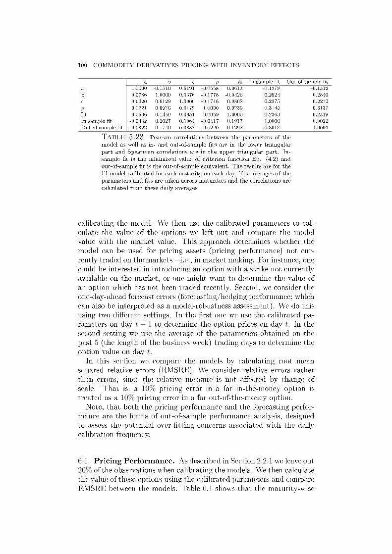
100 COMMODITY DERIVATIVES PRICING WITH INVENTORY EFFECTS
a b c ρ I0 In sample t Out of sample ta 1.0000 -0.1510 0.6191 -0.0558 0.0613 -0.1278 -0.1312b 0.0786 1.0000 0.5376 -0.1778 -0.0426 0.2924 0.2840c 0.6620 0.6129 1.0000 -0.1746 0.0808 0.2375 0.2242ρ 0.0221 0.0976 -0.0179 1.0000 -0.0239 -0.3145 -0.3137I0 0.0536 0.1459 0.0851 0.0059 1.0000 0.2363 0.2319In sample t -0.0332 0.2027 0.1064 -0.0417 0.1917 1.0000 0.9022Out of sample t -0.0322 0.1740 0.0837 -0.0220 0.1298 0.8018 1.0000
Table 5.23. Pearson correlations between the parameters of themodel as well as in- and out-of-sample ts are in the lower triangularpart and Spearman correlations are in the upper triangular part. In-sample t is the minimized value of criterion function Eq. (4.2) andout-of-sample t is the out-of-sample equivalent. The results are for theFI model calibrated for each maturity on each day. The averages of theparameters and ts are taken across maturities and the correlations arecalculated from these daily averages.
calibrating the model. We then use the calibrated parameters to cal-culate the value of the options we left out and compare the modelvalue with the market value. This approach determines whether themodel can be used for pricing assets (pricing performance) not cur-rently traded on the markets i.e., in market making. For instance, onecould be interested in introducing an option with a strike not currentlyavailable on the market, or one might want to determine the value ofan option which has not been traded recently. Second, we consider theone-day-ahead forecast errors (forecasting/hedging performance; whichcan also be interpreted as a model-robustness assessment). We do thisusing two dierent settings. In the rst one we use the calibrated pa-rameters on day t− 1 to determine the option prices on day t. In thesecond setting we use the average of the parameters obtained on thepast 5 (the length of the business week) trading days to determine theoption value on day t.In this section we compare the models by calculating root mean
squared relative errors (RMSRE). We consider relative errors ratherthan errors, since the relative measure is not aected by change ofscale. That is, a 10% pricing error in a far in-the-money option istreated as a 10% pricing error in a far out-of-the-money option.Note, that both the pricing performance and the forecasting perfor-
mance are the forms of out-of-sample performance analysis, designedto assess the potential over-tting concerns associated with the dailycalibration frequency.
6.1. Pricing Performance. As described in Section 2.2.1 we leave out20% of the observations when calibrating the models. We then calculatethe value of these options using the calibrated parameters and compareRMSRE between the models. Table 6.1 shows that the maturity-wise
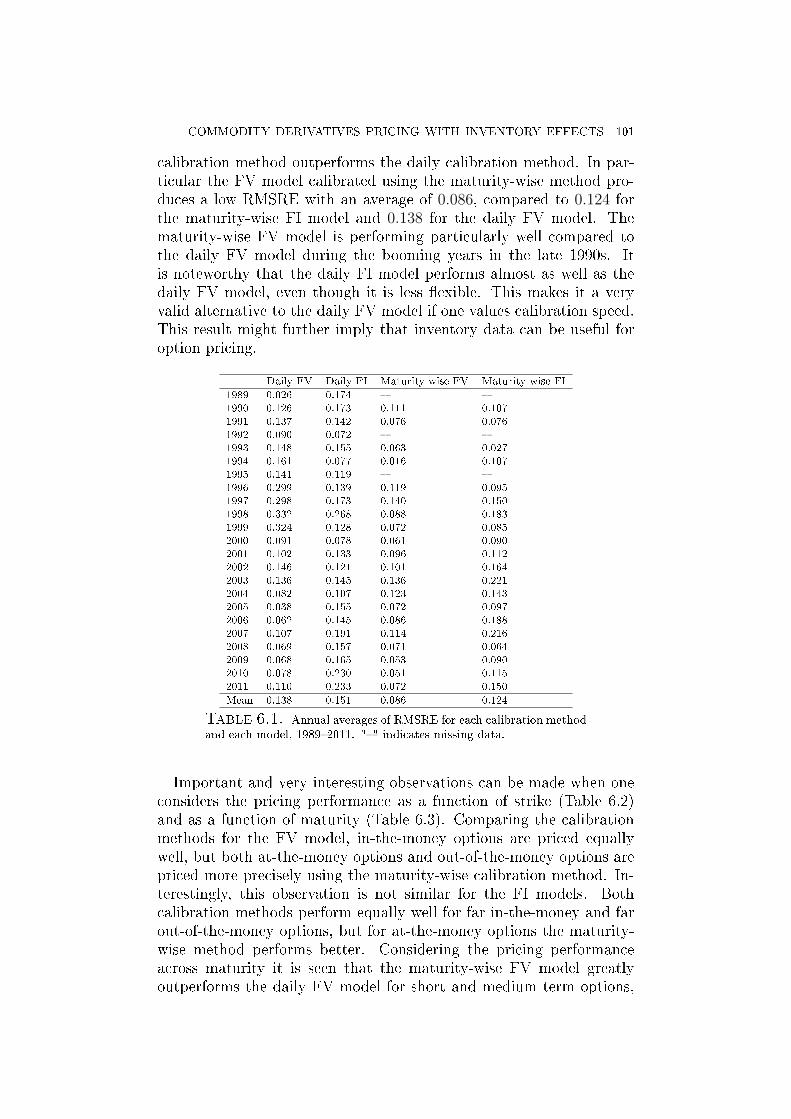
COMMODITY DERIVATIVES PRICING WITH INVENTORY EFFECTS 101
calibration method outperforms the daily calibration method. In par-ticular the FV model calibrated using the maturity-wise method pro-duces a low RMSRE with an average of 0.086, compared to 0.124 forthe maturity-wise FI model and 0.138 for the daily FV model. Thematurity-wise FV model is performing particularly well compared tothe daily FV model during the booming years in the late 1990s. Itis noteworthy that the daily FI model performs almost as well as thedaily FV model, even though it is less exible. This makes it a veryvalid alternative to the daily FV model if one values calibration speed.This result might further imply that inventory data can be useful foroption pricing.
Daily FV Daily FI Maturity-wise FV Maturity-wise FI
1989 0.026 0.174 1990 0.126 0.173 0.111 0.1071991 0.137 0.142 0.076 0.0761992 0.090 0.072 1993 0.148 0.155 0.063 0.0271994 0.161 0.077 0.016 0.1071995 0.141 0.119 1996 0.299 0.139 0.119 0.0951997 0.298 0.173 0.140 0.1501998 0.332 0.268 0.088 0.1831999 0.324 0.128 0.072 0.0852000 0.091 0.078 0.061 0.0902001 0.102 0.133 0.096 0.1122002 0.146 0.121 0.101 0.1642003 0.136 0.145 0.136 0.2212004 0.082 0.107 0.123 0.1432005 0.038 0.155 0.072 0.0972006 0.062 0.145 0.086 0.1882007 0.107 0.191 0.114 0.2162008 0.069 0.157 0.071 0.0642009 0.068 0.165 0.053 0.0902010 0.078 0.230 0.051 0.1152011 0.110 0.233 0.072 0.150
Mean 0.138 0.151 0.086 0.124
Table 6.1. Annual averages of RMSRE for each calibration methodand each model, 19892011. "" indicates missing data.
Important and very interesting observations can be made when oneconsiders the pricing performance as a function of strike (Table 6.2)and as a function of maturity (Table 6.3). Comparing the calibrationmethods for the FV model, in-the-money options are priced equallywell, but both at-the-money options and out-of-the-money options arepriced more precisely using the maturity-wise calibration method. In-terestingly, this observation is not similar for the FI models. Bothcalibration methods perform equally well for far in-the-money and farout-of-the-money options, but for at-the-money options the maturity-wise method performs better. Considering the pricing performanceacross maturity it is seen that the maturity-wise FV model greatlyoutperforms the daily FV model for short and medium term options,

102 COMMODITY DERIVATIVES PRICING WITH INVENTORY EFFECTS
while for longer term options performance is equal. Considering theFI model the maturity-wise calibration outperforms daily calibrationfor short maturity options while it is worse for long maturity options.The weak performance of the daily FI model for short maturity optionsis expected since inventories play only a small role for short maturityoptions.Considering the FV model, these results suggest that the maturity-
wise calibration method should always be preferred for pricing shortmaturity options and out-of-the-money options, while for long matu-rity options and far in-the-money options one can use the computa-tionally cheaper daily calibration method without much loss of pricingperformance.
Moneyness Daily FV Daily FI Maturity-wise FV Maturity-wise FI
K/F < 0.8 0.083 0.129 0.080 0.1310.8 < K/F < 0.9 0.081 0.163 0.082 0.1360.9 < K/F < 1 0.106 0.177 0.085 0.1341 < K/F < 1.1 0.122 0.179 0.075 0.1241.1 < K/F < 1.2 0.132 0.179 0.080 0.1441.2 < K/F 0.141 0.187 0.105 0.185
Mean 0.111 0.169 0.084 0.142
Table 6.2. Averages of RMSRE for each strike interval for bothcalibration methods and both models.
Time-to-maturity Daily FV Daily FI Maturity-wise FV Maturity-wise FI
τ < 30 0.133 0.404 0.029 0.03230 < τ < 90 0.125 0.261 0.052 0.04890 < τ < 180 0.111 0.111 0.073 0.072180 < τ 0.100 0.101 0.100 0.186
Mean 0.117 0.220 0.063 0.084
Table 6.3. Averages of RMSRE for each time to maturity intervalfor both calibration methods and both models.
Overall, we conclude that the daily FI model is fares well for farITM or long-maturity options (with the less parsimonious FV modelsperforming even better), while the maturity-wise FV model is denitelypreferable for far OTM or short-maturity options. This might reectthe broader presence of the fundamental market participants tradingthese instruments with moneyness reecting the intrinsic contractvalue and long-maturity contracts important for, e.g., fuel hedging bythe airlines.
6.2. Forecasting Performance. In practice the choice between mod-els often ultimately depends on their forecasting performance. In thissection we consider one-day-ahead forecasting performance using boththe parameter-set on the previous day and the average of the parameter-sets over the most recent ve trading days. In Table 6.4 we present the
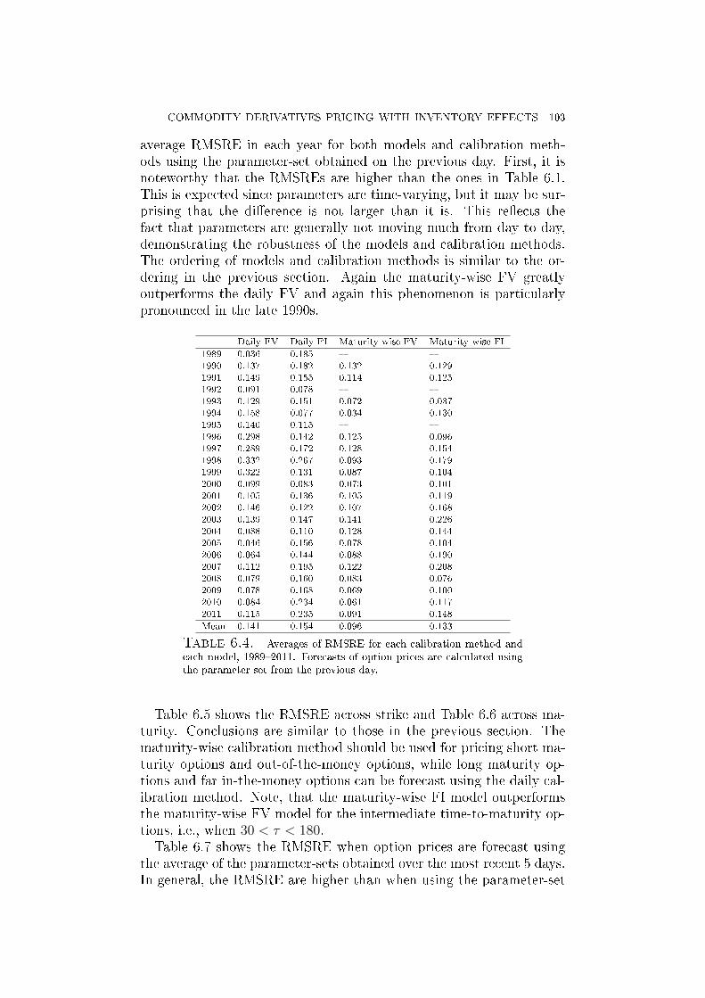
COMMODITY DERIVATIVES PRICING WITH INVENTORY EFFECTS 103
average RMSRE in each year for both models and calibration meth-ods using the parameter-set obtained on the previous day. First, it isnoteworthy that the RMSREs are higher than the ones in Table 6.1.This is expected since parameters are time-varying, but it may be sur-prising that the dierence is not larger than it is. This reects thefact that parameters are generally not moving much from day to day,demonstrating the robustness of the models and calibration methods.The ordering of models and calibration methods is similar to the or-dering in the previous section. Again the maturity-wise FV greatlyoutperforms the daily FV and again this phenomenon is particularlypronounced in the late 1990s.
Daily FV Daily FI Maturity-wise FV Maturity-wise FI
1989 0.036 0.185 1990 0.137 0.182 0.132 0.1291991 0.149 0.155 0.114 0.1251992 0.091 0.078 1993 0.129 0.151 0.072 0.0371994 0.158 0.077 0.034 0.1301995 0.140 0.115 1996 0.298 0.142 0.125 0.0961997 0.289 0.172 0.128 0.1541998 0.332 0.267 0.093 0.1791999 0.322 0.131 0.087 0.1042000 0.099 0.083 0.073 0.1012001 0.105 0.136 0.105 0.1192002 0.146 0.122 0.107 0.1682003 0.139 0.147 0.141 0.2262004 0.088 0.110 0.128 0.1442005 0.046 0.156 0.078 0.1042006 0.064 0.144 0.088 0.1902007 0.112 0.195 0.122 0.2082008 0.079 0.160 0.083 0.0762009 0.078 0.168 0.069 0.1002010 0.084 0.234 0.061 0.1172011 0.115 0.235 0.091 0.148
Mean 0.141 0.154 0.096 0.133
Table 6.4. Averages of RMSRE for each calibration method andeach model, 19892011. Forecasts of option prices are calculated usingthe parameter-set from the previous day.
Table 6.5 shows the RMSRE across strike and Table 6.6 across ma-turity. Conclusions are similar to those in the previous section. Thematurity-wise calibration method should be used for pricing short ma-turity options and out-of-the-money options, while long maturity op-tions and far in-the-money options can be forecast using the daily cal-ibration method. Note, that the maturity-wise FI model outperformsthe maturity-wise FV model for the intermediate time-to-maturity op-tions, i.e., when 30 < τ < 180.Table 6.7 shows the RMSRE when option prices are forecast using
the average of the parameter-sets obtained over the most recent 5 days.In general, the RMSRE are higher than when using the parameter-set

104 COMMODITY DERIVATIVES PRICING WITH INVENTORY EFFECTS
Daily FV Daily FI Maturity-wise FV Maturity-wise FI
K/F < 0.8 0.089 0.133 0.088 0.1360.8 < K/F < 0.9 0.089 0.164 0.092 0.1440.9 < K/F < 1 0.109 0.177 0.089 0.1381 < K/F < 1.1 0.123 0.181 0.083 0.1291.1 < K/F < 1.2 0.136 0.183 0.097 0.1411.2 < K/F 0.149 0.196 0.117 0.174
Mean 0.116 0.172 0.094 0.144
Table 6.5. Averages of RMSRE for each strike interval for bothcalibration methods and each model. Forecasts of option prices arecalculated using the parameter-set from the previous day.
Daily FV Daily FI Maturity-wise FV Maturity-wise FI
τ < 30 0.138 0.403 0.064 0.06630 < τ < 90 0.131 0.264 0.070 0.06690 < τ < 180 0.116 0.116 0.081 0.079180 < τ 0.102 0.105 0.106 0.186
Mean 0.122 0.222 0.080 0.099
Table 6.6. Averages of RMSRE for each time to maturity intervalfor both calibration methods and each model. Forecasts of option pricesare calculated using the parameter-set from the previous day.
from the past day. This suggests that while the model parameters donot change much from day to day, they still change suciently muchthat using information from as far as ve days back is not relevant. Thisshows the importance of using the most recent information (and under-scores the desirability of the daily calibration frequency in practice).The performance loss is particularly pronounced for the maturity-wisecalibration methods and probably reects the fact that in the maturity-wise calibration method parameters are less stable than they are in thedaily calibration, since they are calibrated to contracts with a specicmaturity. The daily-calibrated FI model is now performing much bet-ter than any other model. This reects the fact that parameters aremore stable in the FI model as compared to the FV model. This sta-bility is a desired feature for hedging, since the costs of rebalancing arereduced with less frequent rebalancing.Tables 6.8 - 6.9 show RMSRE across the strike and maturity di-
mensions. For the models calibrated using the daily method the RM-SREs are relatively stable across the strike dimension, while for thematurity-wise calibration they are remarkably lower for at-the-moneyoptions as compared to in- and out-of-the money options. Yet, for anymodel and any calibration method the RMSRE are as low as thoseobserved when using the parameter-set from the previous day. Thisis also the case when considering the RMSRE across maturity for allmodels. In general, these tables suggest that rather than using theaverage of parameter-sets over the most recent period one should usethose calibrated on the previous day.

COMMODITY DERIVATIVES PRICING WITH INVENTORY EFFECTS 105
Daily FV Daily FI Maturity-wise FV Maturity-wise FI
1989 0.052 0.095 1990 0.323 0.188 0.162 3.6281991 0.189 0.162 0.357 2.4521992 0.151 0.056 1993 0.431 0.085 0.077 1.1841994 0.320 0.081 0.133 1.3171995 0.121 0.087 1996 0.416 0.148 0.345 1.8091997 0.575 0.154 0.311 1.4151998 0.523 0.338 0.142 1.0171999 0.455 0.161 0.181 1.6412000 0.149 0.092 0.225 2.4122001 0.180 0.189 0.212 2.0542002 0.241 0.158 0.201 2.1252003 0.156 0.177 0.315 2.3362004 0.128 0.116 0.363 4.2892005 0.055 0.159 0.168 6.5132006 0.067 0.145 0.351 7.2142007 0.126 0.195 0.496 7.5882008 0.084 0.161 0.395 15.0242009 0.089 0.169 0.180 11.1062010 0.093 0.238 0.232 11.1652011 0.121 0.242 0.516 13.141
Mean 0.219 0.156 0.268 4.972
Table 6.7. Averages of RMSRE for each for each calibrationmethod and each model, 19892011. Forecasts of option prices are cal-culated using the average of the parameter set on the past 5 days.
Daily FV Daily FI Maturity-wise FV Maturity-wise FI
K/F < 0.8 0.114 0.139 0.425 17.0610.8 < K/F < 0.9 0.134 0.171 0.397 10.1210.9 < K/F < 1 0.150 0.182 0.256 7.3701 < K/F < 1.1 0.170 0.190 0.257 7.2401.1 < K/F < 1.2 0.210 0.201 0.395 9.4791.2 < K/F < 1.3 0.208 0.215 0.424 13.6411.3 < K/F 0.164 0.183 0.359 10.819
Table 6.8. Averages of RMSRE for each strike interval for bothcalibration methods and each model. Forecasts of option prices arecalculated using the average of the parameter set on the past 5 days.
Daily FV Daily FI Maturity-wise FV Maturity-wise FI
τ < 30 0.148 0.408 0.250 8.04230 < τ < 90 0.153 0.272 0.344 7.87390 < τ < 180 0.158 0.131 0.414 8.065180 < τ 0.169 0.115 0.300 11.969
Mean 0.157 0.232 0.327 8.987
Table 6.9. Averages of RMSRE for each time to maturity intervalfor both calibration methods and each model. Forecasts of option pricesare calculated using the average of the parameter set on the past 5 days.
Overall, we conclude that when the forecasts of option prices arecalculated using the parameter-set from the previous day the maturity-wise models are preferred to daily models and FV models are in general

106 COMMODITY DERIVATIVES PRICING WITH INVENTORY EFFECTS
preferred to FI models. However, we note good performance of the dailyFI model for long-maturity options.When the forecasts of option prices are calculated using the average
of the parameter-set on the past 5 days, the daily models are preferredto maturity-wise models. On average, the daily FI model performs thebest here, which might be related to fundamental factors mentioned inSection 6.1.In general, forecasting the option prices using the parameter-set from
the previous day with the maturity-wise FV model results in the bestperformance.
7. The Black-Scholes Model Benchmark
In the previous sections we have shown that inventory data can beuseful for calibration in terms of t, forecasting and pricing. In orderto investigate this further, we also include the results for the Black-Scholes-Merton (BSM) model (or, the in context of our underlying, aBlack (1976) model) as a benchmark.
7.1. BSMwith Maturity-wise Calibration. The mean and medianstandard deviations are behaving as expected they are around theexpected levels and they clearly show both the dot-com crisis around2001-2002 and the recent credit crisis around 2008-2009. The in-sampleand out-of-sample t errors are signicantly higher (about an orderof magnitude) than for any of our other models, which is of courseexpected, due to the extra exibility in the other models compared toBSM. This demonstrates the relative importance of stochastic volatility(or inventory) over the constant volatility assumption. It is remarkablethat the in-sample t has been very poor since the nancial crisis.Among practitioners, it has been observed that many of the standardtools have not worked well in the recent years perhaps this is just aconrmation of that observation. Out-of-sample t is also much worsein recent years which is very clearly seen in the median results.There is a large dierence between mean and median results for in-
and out-of-sample ts. This indicates that for a lot of the observationsthe model is performing very poorly.
7.2. BSM with Daily Calibration. Again, the σ values are aroundthe expected level. However, in the daily calibration the σ values donot seem to capture the well-known increase in the volatility in 2008-2009 and only weakly capture the volatility increase in the 2001-2002crisis. However, the 2008-2009 crisis is clearly aecting the RMSE.Comparing results with those for the maturity-wise calibration the
RMSEs are substantially higher, which was also the case for all thepreviously discussed models. Naturally, this is still partially a resultof the added exibility of the maturity-wise method, but it conrmsand highlights that using the maturity-wise calibration one can obtain

COMMODITY DERIVATIVES PRICING WITH INVENTORY EFFECTS 107
Year σ In sample t Out of sample t Obs.
1990 0.6049 0.0322 2.4889 111.00001991 0.3545 0.0028 0.2427 138.00001993 0.2397 0.0006 0.7125 52.00001994 0.2436 0.0004 0.6753 126.00001996 0.2724 0.0019 0.6389 442.00001997 0.2206 0.0036 1.1124 366.00001998 0.2633 0.0011 1.0681 843.00001999 0.2884 0.0017 0.6388 1553.00002000 0.3042 0.0025 0.3043 1504.00002001 0.3614 0.0054 0.2648 1275.00002002 0.3540 0.0097 0.6896 1591.00002003 0.3137 0.0156 0.0168 1219.00002004 0.3013 0.0107 0.0483 1510.00002005 0.3117 0.0319 0.1006 2246.00002006 0.2594 0.0774 0.0943 2549.00002007 0.2453 0.0890 0.1545 2247.00002008 0.3394 0.0767 0.5570 1779.00002009 0.3982 0.1868 0.2645 1558.00002010 0.2990 0.2332 0.3830 2139.00002011 0.2803 0.2363 0.2448 847.0000
0.3056 0.0692 0.3421 1204.7500
Table 7.1. The mean of the parameter values and ts for each yearusing the number of observations shown in the last column. In-sample tis the minimized value of criterion function Eq. (4.2) and out-of-samplet is the out-of-sample equivalent. The last row shows the mean in thefull sample period. The results are for the BSM model calibrated foreach maturity on each day.
Year σ In sample t Out of sample t Obs.
1990 0.1633 0.1029 17.5010 111.00001991 0.1631 0.0060 1.1298 138.00001993 0.1080 0.0005 1.9332 52.00001994 0.0959 0.0003 2.0229 126.00001996 0.0869 0.0101 5.0996 442.00001997 0.1160 0.0133 2.4754 366.00001998 0.1502 0.0033 2.3745 843.00001999 0.1197 0.0058 1.9187 1553.00002000 0.0843 0.0072 2.9820 1504.00002001 0.1088 0.0102 6.0607 1275.00002002 0.0685 0.0143 14.3895 1591.00002003 0.0552 0.0125 0.0159 1219.00002004 0.0616 0.0123 0.4902 1510.00002005 0.0541 0.0594 0.6588 2246.00002006 0.0274 0.0855 0.3301 2549.00002007 0.0361 0.0810 3.0003 2247.00002008 0.1293 0.1113 7.4808 1779.00002009 0.1236 0.1754 2.6764 1558.00002010 0.0339 0.1534 3.8603 2139.00002011 0.0351 0.1909 0.2040 847.0000
0.0740 0.0667 3.3796 1204.7500
Table 7.2. Standard deviations of the parameter values and ts forthe maturity-wise calibrated BSM model, 1988-2011, using the numberof observations shown in the last column. In sample t is the minimizedvalue of criterion function Eq. (4.2) and out of sample t is the out ofsample equivalent.
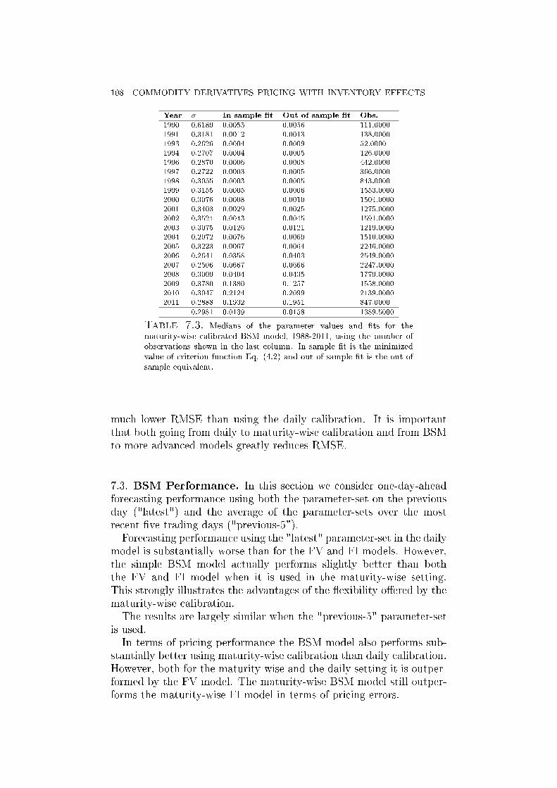
108 COMMODITY DERIVATIVES PRICING WITH INVENTORY EFFECTS
Year σ In sample t Out of sample t Obs.
1990 0.6189 0.0055 0.0056 111.00001991 0.3181 0.0012 0.0013 138.00001993 0.2626 0.0004 0.0009 52.00001994 0.2707 0.0004 0.0005 126.00001996 0.2870 0.0006 0.0008 442.00001997 0.2722 0.0003 0.0005 366.00001998 0.3055 0.0003 0.0005 843.00001999 0.3155 0.0005 0.0006 1553.00002000 0.3076 0.0008 0.0010 1504.00002001 0.3403 0.0029 0.0025 1275.00002002 0.3524 0.0043 0.0045 1591.00002003 0.3075 0.0126 0.0121 1219.00002004 0.2972 0.0076 0.0069 1510.00002005 0.3223 0.0067 0.0064 2246.00002006 0.2641 0.0358 0.0403 2549.00002007 0.2506 0.0667 0.0666 2247.00002008 0.3009 0.0404 0.0435 1779.00002009 0.3780 0.1380 0.1257 1558.00002010 0.3047 0.2124 0.2099 2139.00002011 0.2888 0.1932 0.1951 847.0000
0.2981 0.0139 0.0158 1389.5000
Table 7.3. Medians of the parameter values and ts for thematurity-wise calibrated BSM model, 1988-2011, using the number ofobservations shown in the last column. In sample t is the minimizedvalue of criterion function Eq. (4.2) and out of sample t is the out ofsample equivalent.
much lower RMSE than using the daily calibration. It is importantthat both going from daily to maturity-wise calibration and from BSMto more advanced models greatly reduces RMSE.
7.3. BSM Performance. In this section we consider one-day-aheadforecasting performance using both the parameter-set on the previousday ("latest") and the average of the parameter-sets over the mostrecent ve trading days ("previous-5").Forecasting performance using the "latest" parameter-set in the daily
model is substantially worse than for the FV and FI models. However,the simple BSM model actually performs slightly better than boththe FV and FI model when it is used in the maturity-wise setting.This strongly illustrates the advantages of the exibility oered by thematurity-wise calibration.The results are largely similar when the "previous-5" parameter-set
is used.In terms of pricing performance the BSM model also performs sub-
stantially better using maturity-wise calibration than daily calibration.However, both for the maturity-wise and the daily setting it is outper-formed by the FV model. The maturity-wise BSM model still outper-forms the maturity-wise FI model in terms of pricing errors.

COMMODITY DERIVATIVES PRICING WITH INVENTORY EFFECTS 109
Year σ In sample t Out of sample t Obs.
1989 0.2251 0.0012 0.4290 201.00001990 0.3258 0.0740 0.2206 159.00001991 0.2246 0.0107 0.0104 198.00001992 0.1824 0.0024 0.0314 243.00001993 0.1753 0.0054 0.0061 173.00001994 0.2192 0.0136 0.0141 219.00001995 0.1596 0.0131 0.0144 234.00001996 0.1748 0.0464 0.0467 189.00001997 0.2072 0.0512 0.0579 139.00001998 0.2099 0.1015 0.1106 151.00001999 0.2942 0.0691 0.0706 161.00002000 0.2905 0.0866 0.0860 241.00002001 0.3143 0.1034 0.1014 221.00002002 0.3281 0.1113 0.1101 227.00002003 0.3019 0.1113 0.1124 226.00002004 0.2831 0.2334 0.2337 238.00002005 0.3009 0.4141 0.4061 250.00002006 0.2536 0.2280 0.2274 237.00002007 0.2275 0.5660 4.4852 220.00002008 0.2200 0.7521 6.8730 33.00002010 0.2758 0.8537 15.9218 114.00002011 0.2493 0.8631 0.8533 20.0000
0.2494 0.1552 0.8632 186.0909
Table 7.4. Means of the parameter values and ts for the daily cli-brated BSM model, 1988-2011, using the number of observations shownin the last column. In-sample t is the minimized value of criterionfunction Eq. (4.1) and out-of-sample t is the out-of-sample equivalent.
We see that the BSM is only performing quite well for at-the-moneyoptions, while it performs the worst of all models using any calibrationmethod for the far in-the-money options.BSM performs about equally well in the maturity-wise setting inde-
pendently of maturity. Since both the FV and FI models are performingsubstantially better for short-maturity options than for long-maturityoptions, these models are greatly outperforming the BSM model forshort-maturity options while the BSM model performs no worse thanthe FV model and better than the FI model for long-maturity options.In conclusion, BSM works quite well for ATM options (equally well
independent of time-to-maturity). However, it performs signicantlyworse than the more advanced models for all the other types of options in particular for the far in-the-money options. This shows that sto-chastic volatility or, alternatively, inventory data, are useful for pricingoptions out-of-sample, both in the cross-section (pricing performance)and ahead in time (forecasting performance).
8. Conclusion
We conrm the empirical results in the literature and nd a negativerelationship between inventory and futures prices. At the same time, we

110 COMMODITY DERIVATIVES PRICING WITH INVENTORY EFFECTS
Year σ In sample t Out of sample t Obs.
1989 0.0757 0.0010 1.5669 201.00001990 0.1800 0.1437 1.1272 159.00001991 0.0581 0.0277 0.0298 198.00001992 0.0246 0.0048 0.4489 243.00001993 0.0259 0.0079 0.0106 173.00001994 0.0172 0.0062 0.0077 219.00001995 0.0117 0.0050 0.0088 234.00001996 0.0303 0.0291 0.0316 189.00001997 0.0201 0.0289 0.0413 139.00001998 0.0237 0.0434 0.0559 151.00001999 0.0372 0.0303 0.0357 161.00002000 0.0183 0.0504 0.0541 241.00002001 0.0463 0.0916 0.0894 221.00002002 0.0232 0.0480 0.0553 227.00002003 0.0277 0.0991 0.0979 226.00002004 0.0351 0.1700 0.1743 238.00002005 0.0160 0.1291 0.1416 250.00002006 0.0186 0.1027 0.1077 237.00002007 0.0090 0.1791 19.9639 220.00002008 0.0035 0.1164 24.5729 33.00002010 0.0144 0.1038 36.8647 114.00002011 0.0019 0.0529 0.0770 20.0000
0.0335 0.0668 2.4958 186.0909
Table 7.5. Standard deviations of the parameter values and tsfor the BSM model calibrated daily, 1988-2011, using the number ofobservations shown in the last column. In-sample t is the minimizedvalue of criterion function Eq. (4.1) and out-of-sample t is the out-of-sample equivalent.
nd an interesting non-linear time-structure of the stochastic inventoryprocess.Using a maturity-wise calibration approach improves substantially
on both in- and out-of-sample pricing errors compared to a daily cali-bration.Using the maturity-wise calibration approach the FI model only per-
forms slightly worse than the FV model, which contains one extra pa-rameter to calibrate especially worth noting is an interesting trade-obetween parameter stability (and, consequently, hedging-performance,which we attribute to parsimony) and pricing-performance.We nd that the FI model often performs well in cases associated
with fundamentals-driven prices, i.e., for the contracts of high intrinsicvalue or with long-maturity (where inventories may be an importantlong-term factor).We believe that the extended, three-factor models might oer a good
platform for further study of the necessary ne-tuning of the modeledrelationships between the price, volatility, and inventory in order toachieve the optimal performance for a given market and application.

COMMODITY DERIVATIVES PRICING WITH INVENTORY EFFECTS 111
Year σ In sample t Out of sample t Obs.
1989 0.2362 0.0009 0.0009 201.00001990 0.2318 0.0068 0.0060 159.00001991 0.2033 0.0022 0.0022 198.00001992 0.1761 0.0008 0.0009 243.00001993 0.1737 0.0016 0.0018 173.00001994 0.2185 0.0139 0.0126 219.00001995 0.1587 0.0124 0.0118 234.00001996 0.1637 0.0424 0.0384 189.00001997 0.2110 0.0483 0.0465 139.00001998 0.2058 0.0940 0.0999 151.00001999 0.2783 0.0662 0.0648 161.00002000 0.2930 0.0756 0.0709 241.00002001 0.3119 0.0608 0.0594 221.00002002 0.3272 0.1019 0.0986 227.00002003 0.2912 0.0736 0.0765 226.00002004 0.2771 0.1779 0.1692 238.00002005 0.2998 0.3989 0.3833 250.00002006 0.2526 0.2159 0.2128 237.00002007 0.2284 0.5406 0.5527 220.00002008 0.2198 0.7520 0.7361 33.00002010 0.2696 0.8706 0.8768 114.00002011 0.2496 0.8674 0.8470 20.0000
0.2429 0.0608 0.0619 210.0000
Table 7.6. Medians of the parameter values and ts for the dailyclibrated BSM model, 1988-2011, using the number of observationsshown in the last column. In-sample t is the minimized value of crite-rion function Eq. (4.1) and out-of-sample t is the out-of-sample equiv-alent.
BSM
1989 0.041990 0.191991 0.171992 0.061993 0.111994 0.141995 0.141996 0.261997 0.261998 0.351999 0.222000 0.222001 0.222002 0.222003 0.252004 0.242005 0.202006 0.172007 0.282008 0.352009 0.342010 0.212011 0.26
Mean 0.21
Table 7.7. Averages of RMSRE for BSM model, 19892011. Fore-casts of option prices are calculated using the parameter-set from theprevious day.

112 COMMODITY DERIVATIVES PRICING WITH INVENTORY EFFECTS
BSM
1989 0.0511990 0.1941991 0.1821992 0.0641993 0.1121994 0.1401995 0.1361996 0.2581997 0.2481998 0.3501999 0.2192000 0.2232001 0.2232002 0.2202003 0.2502004 0.2412005 0.2032006 0.1622007 0.2742008 0.3392009 0.3282010 0.2042011 0.254
Mean 0.212
Table 7.8. Averages of RMSRE for BSM model, 19892011. Fore-casts of option prices are calculated using the average of the parameterset on the past 5 days.
References
Bakshi, G., C. Cao, and Z. Chen (1997). Empirical performance ofalternative option pricing models. Journal of Finance 52 (5), 200349.
Barone-Adesi, G. and R. E. Whaley (1987). Ecient analytic approxi-mation of american option values. Journal of Finance 42 (2), 30120.
Benhamou, E., E. Gobet, and M. Miri (2010). Time dependent hestonmodel. SIAM Journal on Financial Mathematics 1 (1), 289.
Bessembinder, H., J. F. Coughenour, P. J. Seguin, and M. M. Smoller(1995). Mean reversion in equilibrium asset prices: Evidence fromthe futures term structure. Journal of Finance 50 (1), 36175.
Black, F. (1976). The pricing of commodity contracts. Journal ofFinancial Economics 3 (1-2), 167179.
Brennan, M. J. (1958). The supply of storage. The American EconomicReview 48 (1), 5072.
Brennan, M. J. (1991). The Price of Convenience and the Valuationof Commodity Contingent Claims. In: Lund, D., and Oksendal, B.(eds), Stochastic Models and Option Values. North Holland.
Broadie, M., M. Chernov, and M. Johannes (2007). Model specica-tion and risk premia: Evidence from futures options. Journal ofFinance 62 (3), 14531490.

COMMODITY DERIVATIVES PRICING WITH INVENTORY EFFECTS 113
Christoersen, P., S. Heston, and K. Jacobs (2009). The shape andterm structure of the index option smirk: Why multifactor stochasticvolatility models work so well. Management Science 55 (12), 19141932.
Cortazar, G. and E. S. Schwartz (1994). The valuation of commodity-contingent claims. The Journal of Derivatives 1 (4), 2739.
Fama, E. F. and K. R. French (1987). Commodity futures prices: Someevidence on forecast power, premiums, and the theory of storage. TheJournal of Business 60 (1), 5573.
Fama, E. F. and K. R. French (1988). Business cycles and the behaviorof metals prices. Journal of Finance 43 (5), 107593.
Gabillon, J. (1991). The term structures of oil futures prices. OxfordInstitute for Energy Studies.
Geman, H. (2005). Commodities and Commodity Derivatives : Mod-elling and Pricing for Agriculturals, Metals and Energy. Wiley Fi-nance.
Geman, H., N. El Karoui, and J. C. Rochet (1995). Changes ofnuméraire, changes of probability measures and pricing of options.Journal of Applied Probability 32, 443458.
Geman, H. and V. Nguyen (2005). Soybean inventory and forwardcurve dynamics. Management Science 51 (7), 10761091.
Geman, H. and S. Ohana (2009). Forward curves, scarcity and pricevolatility in oil and natural gas markets. Energy Economics 31 (4),576585.
Gibson, R. and E. S. Schwartz (1990). Stochastic convenience yieldand the pricing of oil contingent claims. Journal of Finance 45 (3),95976.
Heston, S. L. (1993). A closed-form solution for options with stochasticvolatility with applications to bond and currency options. Review ofFinancial Studies 6 (2), 32743.
Jing-Zhi and L. Wu (2004). Specication analysis of option pricingmodels based on time-changed lévy processes. The Journal of Fi-nance 59 (3), 14051439.
Ju, N. and R. Zhong (1999). An approximate formula for pricing amer-ican options. The Journal of Derivatives 7 (2), 3140.
Kaldor, N. (1939). Speculation and economic stability. Review of Eco-nomic Studies 7 (1), 127.
Lindström, E., J. Ströjby, M. Brodén, M. Wiktorsson, and J. Holst(2008, February). Sequential calibration of options. Comput. Stat.Data Anal. 52, 28772891.
Ng, V. K. and S. C. Pirrong (1994). Fundamentals and volatility:Storage, spreads, and the dynamics of metals prices. The Journal ofBusiness 67 (2), 20330.
Ross, S. (1997). Hedging long run commitments: Exercises in incom-plete market pricing. Economic Notes 26 (2), 99132.

114 COMMODITY DERIVATIVES PRICING WITH INVENTORY EFFECTS
Routledge, B. R., D. J. Seppi, and C. S. Spatt (2000). Equilibriumforward curves for commodities. Journal of Finance 55 (3), 12971338.
Schwartz, E. S. (1997). The stochastic behavior of commodity prices:Implications for valuation and hedging. Journal of Finance 52 (3),92373.
Telser, L. G. (1958). Futures trading and the storage of cotton andwheat. Journal of Political Economy 66 (3), 233255.
Trolle, A. B. and E. S. Schwartz (2009). Unspanned stochastic volatil-ity and the pricing of commodity derivatives. Review of FinancialStudies 22 (11), 44234461.
Working, H. (1949). The theory of the price of storage. AmericanEconomic Review 39, 12541262.
Zhu, J. (2000). Modular Pricing of Options. Springer, New York.

COMMODITY DERIVATIVES PRICING WITH INVENTORY EFFECTS 115
9. Appendix A: Three-Factor Models and their
Semi-Closed-Form Solutions
9.1. FVI model. In the above model formulation we implementedinventory in the price dynamics through a deterministic formula. Analternative approach, and a more exible one, is to include inventoryas a third factor such that the model (FVI) can be formulated as
dFt =√VtF
βt dW
Ft ,
dVt = aV (bV It − Vt) dt+ cV√VtdW
Vt ,
dIt = aI (bI − It) dt+ cIIγt dW
It ,[
W F ,W V]t
= ρFV t,[W F ,W I
]t
= ρFIt,[W V ,W I
]t
= ρV It.
In this model we let inventories inuence the dynamics of the futuresthrough the long run value of stochastic volatility and through thecorrelation dynamics.
9.2. Heston model. The Heston (1993) model assumes that S, theprice of the asset, is determined by:
dSt = µSt dt+√νtSt dW
St (9.1)
dνt = κ(θ − νt) dt+ ξ√νt dW
νt (9.2)
d[W S,W ν ]t = ρtdt, (9.3)
where ν, the instantaneous variance, is a CIR process. Note, thatthe particular form of the drift term in a CIR process induces mean-reversion of the volatility process (which ts the empirical evidencebetter than a non-reverting non-zero drift).Benhamou et al. (2010) consider a time-dependent Heston model,
with time-varying θt and ξt.
9.3. FVV model. We consider a model for the price of a future con-tract in a Heston type model augmented by an additional process forvolatility (which can alternatively be an inventory factor, leading toanother variation of FVI model). In the case for stocks the model haspreviously been considered in a very general setup in Zhu (2000) and isapplied for calibrating stock options in Christoersen et al. (2009) in aless general setup. As in Christoersen et al. (2009) we make simplify-ing assumptions on the correlation structure and formulate the model

116 COMMODITY DERIVATIVES PRICING WITH INVENTORY EFFECTS
as
dFt =√V 1t dW
QF1,t +
√V 2t dW
QF2,t
dV 1t = aV 1
(bV 1 − V 1
t
)dt+ cV 1
√V 1t dW
QV 1,t
dV 2t = aV 2
(bV 2 − V 2
t
)dt+ cV 2
√V 2t dW
QV 2,t
d[WQF1,W
QV 1]t = ρF1V 1dt
d[WQF2,W
QV 2]t = ρF2V 2dt
d[WQF1,W
QV 2]t = 0
d[WQF2,W
QV 1]t = 0
d[WQF1,W
QF2]t = 0
d[WQV 1,W
QV 2]t = 0
The correlation matrix ρ of the random sources(WQF1,W
QF2,W
QV 1,W
QV 2
)
can be summarized as
ρ :=
1 0 ρF1V 1 00 1 0 ρF2V 2
ρF1V 1 0 1 00 ρF2V 2 0 1
.
European call options are valued via Fourier analysis and formulaspresented in Christoersen et al. (2009).
9.4. FVL model. We consider a model for the price of a future con-tract in a Heston type model augmented by a latent process. Themodel is formulated in the risk-neutral world as
dFt =√Vt dW
QF,t,
dVt = aV (bV − Vt) dt+ cV√VtdW
QV,t, (9.4)
dLt = aL (bL − Lt) dt+ cL√LtdW
QL,t,
d[WQF ,W
QV ]t = ρFV dt,
d[WQF ,W
QL ]t = ρFLdt,
d[WQV ,W
QL ]t = ρV Ldt.
9.4.1. The Option Valuation Formulas. The correlation matrix ρ of the
random sources(WQF ,W
QV ,W
QL
)is
ρ :=
1 ρV L ρFVρV L 1 ρFLρFV ρFL 1
,

COMMODITY DERIVATIVES PRICING WITH INVENTORY EFFECTS 117
and introducing Wiener processes Wα and Wβ both mutually indepen-
dent and independent of WQL , W
QV , and W
QF the Cholesky decomposi-
tion yields
1 0 0
ρV L√
1− ρV L2 0
ρFVρFL−ρFV ρV L√
1−ρV L2
√(ρFL−ρFV ρV L)2
ρV L2−1− ρFV 2 + 1
which allows us to write
WQV = WQ
V ,
WQL = ρV LW
QV +
√1− ρ2
V LWα = ρV LWQV + ραWα, (9.5)
WQF = ρFVW
QV +
ρFL − ρFV ρV L√1− ρ2
V L
WQL +
√ρ2FL + ρ2
FV + ρ2V L − 2ρFLρFV ρV L − 1
ρ2V L − 1
Wβ
= ρFVWQV + ργW
QL + ρβWβ, (9.6)
where
ρα =√
1− ρ2V L,
ρβ =
√ρ2FL + ρ2
FV + ρ2V L − 2ρFLρFV ρV L − 1
ρ2V L − 1
,
ργ =ρFL − ρFV ρV L√
1− ρ2V L
.
Dene Xt = ln (Ft); applying Ito's lemma yields
dXt = −1
2Vtdt+
√VtdW
QF,t. (9.7)
We dene the Radon-Nikodym derivative of change from the risk-neutral measure Q to the measure QF associated with numeraire Ft;see Geman et al. (1995)
gFt :=dQF
dQ|Ft =
β0FtβtF0
= exp
−∫ t
0
r (s) ds
FtF0
, (9.8)
where
βt := exp
∫ t
0
rds
.
We know that a discounted price process of European-style option ona futures contract F with strike price K is a martingale under the

118 COMMODITY DERIVATIVES PRICING WITH INVENTORY EFFECTS
risk-neutral measure Q, i.e.(Cβ
)∈M (Q). Hence
C (F0, T ;K)
β0
= EQ0
[C (FT , T ;K)
βT
]
= EQ0
[(FT −K)+
βT
].
Rearranging, we have (where we drop conditioning since we are at timet = 0)
C (F0, T ;K) = EQ
[β0
βT(FT −K) · 1(FT>K)
]
= EQ
[β0
βTFT · 1(FT>K)
]− EQ
[β0
βTK · 1(FT>K)
],
Let Bt,T := EQt
[βtβT
]denote the value of a zero-coupon bond at time
t and maturity at time T . Then the Radon-Nikodym derivative tochange from the risk-neutral measure Q to the forward measure QB isdened by
gBt :=dQB
dQ|Ft =
β0BT,T
βTB0,T
. (9.9)
Note BT,T = 1. We can now apply the Radon-Nikodym derivative from(9.8) to the rst term and the Radon-Nikodym derivative from (9.9) tothe second term
C (F0, T ;K) = EQ[F0g
FT · 1(FT>K)
]− EQ
[B0,Tg
BTK · 1(FT>K)
]
= F0EQ[gFT · 1(FT>K)
]−B0,TKE
Q[gBT · 1(FT>K)
]
= F0QF (XT > k)−B0,TKQ
B (XT > k) , (9.10)
where k = ln (K) and Q∗ (XT > k) is the probability that the optionnishes in-the-money (ITM), under the Q∗ measure.Using the inverse Fourier transform, the European-style call option
valuation formula (9.10) can be written as (where we insert the ITMprobabilities)
C (F0, T ;K) = F0QF (XT > k)−B0,TKQ
B (XT > k) ,
where
QF (XT > k) =1
2+
1
π
∫ ∞
0
Re
[ϕF (φ)
exp(−iφk)
iφ
]dφ
and
QB (XT > k) =1
2+
1
π
∫ ∞
0
Re
[ϕB (φ)
exp(−iφk)
iφ
]dφ.

COMMODITY DERIVATIVES PRICING WITH INVENTORY EFFECTS 119
Similarly, the European-style put option valuation formula becomes(where we insert the OTM probabilities)
P (F0, T ;K) = B0,TKQB (XT < k)− F0Q
F (XT < k) ,
where
QF (XT < k) =1
2− 1
π
∫ ∞
0
Re
[ϕF (φ)
exp(−iφk)
iφ
]dφ
and
QB (XT < k) =1
2− 1
π
∫ ∞
0
Re
[ϕB (φ)
exp(−iφk)
iφ
]dφ.
Note that we can also obtain the pricing formula for put options byusing put-call parity.
9.4.2. Characteristic function ϕF . To calculate the option prices weare interested ITM/OTM probabilities under the QF measure. Thecharacteristic function under the probability measure QF is dened by
ϕF (φ) := EQF [exp iφXT] .Using the Radon-Nikodym derivative (9.8), we can obtain the the char-acteristic function under the original risk-neutral measure
ϕF (φ) = EQ[gFT exp iφXT
]. (9.11)
Since we assume a constant interest rate
gFT = exp −rT +XT −X0 ,and substituting this into (9.11) yields
ϕF (φ) ≡ EQ [exp −rT +XT −X0 exp iφXT]= EQ [exp −rT −X0 + (1 + iφ)XT] . (9.12)
From (9.7) we know that we can formulate XT as
XT = X0 −1
2
∫ T
0
Vtdt+
∫ T
0
√VtdW
QF,t.
Substituting this into (9.12) yields
ϕF (φ) = EQ
[exp iφX0 − rT exp
(1 + iφ)
(−1
2
∫ T
0
Vtdt+
∫ T
0
√VtdW
QF,t
)]
= EQ
[exp
RF
exp
AF∫ T
0
Vtdt+BF
∫ T
0
√VtdW
QF,t
],
where RF = iφX0−rT , AF = −12BF , and BF = (1 + iφ). Substituting
(9.6) for dWQF,t yields
ϕF (φ) = EQ
[exp
RF
exp
AF∫ T
0Vtdt+BFρFV
∫ T0
√VtdW
QV,t
+BFργ∫ T
0
√VtdW
QL,t +BFρβ
∫ T0
√VtdWβ
].

120 COMMODITY DERIVATIVES PRICING WITH INVENTORY EFFECTS
Substituting (9.5) for dWQL,t yields
ϕF (φ) = EQ
exp
RF
exp
AF∫ T
0Vtdt+BFρFV
∫ T0
√VtdW
QV,t
+BFργρV L∫ T
0
√VtdW
QV,t
+BFργρα∫ T
0
√VtdWα +BFρβ
∫ T0
√VtdWβ
= EQ
[exp
RF
exp
AF∫ T
0Vtdt+
(BFρFV +BFργρV L
) ∫ T0
√VtdW
QV,t
+BFργρα∫ T
0
√VtdWα +BFρβ
∫ T0
√VtdWβ
]
= EQ
[exp
RF
exp
AF∫ T
0Vtdt+BF
V
∫ T0
√VtdW
QV,t
+BFα
∫ T0
√VtdWα +BF
β
∫ T0
√VtdWβ
],
where BFV = BFρFV +BFργρV L, B
Fα = BFργρα, and B
Fβ = BFρβ. We
can now rewrite the characteristic function as11
ϕF (φ) = EQ
exp
RF
expBFV
∫ T0
√VtdW
QV,t
× expAF∫ T
0Vtdt+BF
α
∫ T0
√VtdWα +BF
β
∫ T0
√VtdWβ
,
and since Wα and Wβ are independent Wiener processes and I1(T ) =∫ T0
√VtdWα and I2(T ) =
∫ T0
√VtdWβ are martingales under Q measure
it follows (where the E operator acts solely and separately under the
11To show this several observations need to be made. In general, consider twodependent stochastic variables, X and Y and dene µX := E
[eX]= eµX . Further
dene variables Zi, i = 1, 2, 3, mutually independent and independent of X and Y .Then
E[eZ1XeY XeZ2XeZ3X
]= E
[E[eZ1XeY XeZ2XeZ3X |X
]]
= E[E[eY X |X
]E[eZ1XeZ2XeZ3X |X
]]
= E
[E[eY X |X
]E
[3∏
i=1
eZiX |X]]
= E
[E[eY X |X
] 3∏
i=1
eµZiµX
]
= E
[E
[eY X
3∏
i=1
eµZiµX |X
]]
= E
[eY X
3∏
i=1
eµZiµX
].
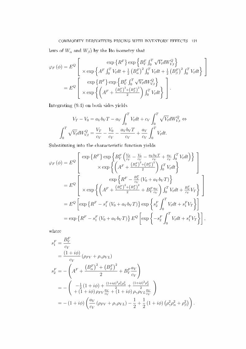
COMMODITY DERIVATIVES PRICING WITH INVENTORY EFFECTS 121
laws of Wα and Wβ) by the Ito isometry that
ϕF (φ) = EQ
exp
RF
expBFV
∫ T0
√VtdW
QV,t
× expAF∫ T
0Vtdt+ 1
2
(BFα
)2 ∫ T0Vtdt+ 1
2
(BFβ
)2 ∫ T0Vtdt
= EQ
expRF
expBFV
∫ T0
√VtdW
QV,t
× exp
(AF +
(BFα )2+(BFβ )
2
2
)∫ T0Vtdt
.
Integrating (9.4) on both sides yields
VT − V0 = aV bV T − aV∫ T
0
Vtdt+ cV
∫ T
0
√VtdW
QV,t ⇔
∫ T
0
√VtdW
QV,t =
VTcV− V0
cV− aV bV T
cV+aVcV
∫ T
0
Vtdt.
Substituting into the characteristic function yields
ϕF (φ) = EQ
expRF
expBFV
(VTcV− V0
cV− aV bV T
cV+ aV
cV
∫ T0Vtdt
)
× exp
(AF +
(BFα )2+(BFβ )
2
2
)∫ T0Vtdt
= EQ
expRF − BFV
cV(V0 + aV bV T )
× exp
(AF +
(BFα )2+(BFβ )
2
2+BF
VaVcV
)∫ T0Vtdt+
BFVcVVT
= EQ
[exp
RF − sF1 (V0 + aV bV T )
exp
sF2
∫ T
0
Vtdt+ sF1 VT
]
= expRF − sF1 (V0 + aV bV T )
EQ
[exp
−sF2
∫ T
0
Vtdt+ sF1 VT
],
where
sF1 =BFV
cV
=(1 + iφ)
cV(ρFV + ργρV L)
sF2 = −(AF +
(BFα
)2+(BFβ
)2
2+BF
V
aVcV
)
= −(−1
2(1 + iφ) +
(1+iφ)2ρ2γρ
2α
2+
(1+iφ)2ρ2β
2+ (1 + iφ) ρFV
aVcV
+ (1 + iφ) ργρV LaVcV
)
= − (1 + iφ)
(aVcV
(ρFV + ργρV L)− 1
2+
1
2(1 + iφ)
(ρ2γρ
2α + ρ2
β
)).

122 COMMODITY DERIVATIVES PRICING WITH INVENTORY EFFECTS
We need to calculate the following expectation
y (VT , T ) = EQ
[exp
−sF2
∫ T
0
Vtdt+ sF1 VT
].
According to the Feynman-Kac theorem the expected value satisesthe one-dimensional PDE
∂y
∂T= −sF2 V y + aV (bV − V )
∂y
∂V+
1
2σ2V
∂2y
∂V 2,
with the boundary condition
y (V0, 0) = expsF1 V0
.
The solution to this PDE is given by
y = exp H1 (T )V0 +H2 (T ) ,where
H1 =1
ψ2
[ψ1s
F1
(1 + e−ψ1T
)−(1− e−ψ1T
) (2sF2 + aV s
F1
)]
H2 =2aV bVc2V
ln
[2ψ1
ψ2
exp
1
2(aV − ψ1)T
],
and
ψ1 =√a2V + 2c2
V sF2
ψ2 = 2ψ1e−ψ1T +
(aV + ψ1 − c2
V sF1
) (1− e−ψ1T
).
9.4.3. Characteristic function ϕB. To calculate the option prices weare interested ITM/OTM probabilities under the QB measure. Thecharacteristic function under the probability measure QB is dened by
ϕB (φ) := EQB [exp iφXT] .Using gBT we can obtain the the characteristic function under the orig-inal risk-neutral measure Q
ϕB (φ) = EQ[gBT exp iφXT
], (9.13)
since we assume a constant interest rate
gBT =β0BT,T
βTB0,T
=β0
βTβT
βTβ0
βT
= 1,
and substituting this into (9.13) yields
ϕB (φ) ≡ EQ [exp iφXT] (9.14)
Integrating (9.7) we know that
XT = X0 −1
2
∫ T
0
Vtdt+
∫ T
0
√VtdW
QF,t.

COMMODITY DERIVATIVES PRICING WITH INVENTORY EFFECTS 123
Substituting into (9.14) gives
ϕB (φ) = EQ
[exp
iφ
(X0 −
1
2
∫ T
0
Vtdt+
∫ T
0
√VtdW
QF,t
)],
= EQ
[exp iφX0 exp
−1
2iφ
∫ T
0
Vtdt+ iφ
∫ T
0
√VtdW
QF,t
],
Substituting (9.6) for dWQF,t yields
ϕB (φ) = EQ
[exp iφX0 exp
−1
2iφ∫ T
0Vtdt
+iφ∫ T
0
√Vt
(ρFV dW
QV,t + ργdW
QL,t + ρβdWβ
)]
= EQ
[exp iφX0 exp
−1
2iφ∫ T
0Vtdt+ iφρFV
∫ T0
√VtdW
QV,t
+iφργ∫ T
0
√VtdW
QL,t + iφρβ
∫ T0
√VtdWβ
].
Substituting (9.5) for dWQL,t yields
ϕB (φ) = EQ
exp iφX0 exp
−12iφ∫ T
0Vtdt+ iφρFV
∫ T0
√VtdW
QV,t
+iφργρV L∫ T
0
√VtdW
QV,t
+iφργρα∫ T
0
√VtdWα + iφρβ
∫ T0
√VtdWβ
= EQ
exp iφX0 exp
−12iφ∫ T
0Vtdt
+ (iφρFV + iφργρV L)∫ T
0
√VtdW
QV,t
+iφργρα∫ T
0
√VtdWα + iφρβ
∫ T0
√VtdWβ
= EQ
[exp iφX0 exp
AB∫ T
0Vtdt+BB
V
∫ T0
√VtdW
QV,t
+BBα
∫ T0
√VtdWα +BB
β
∫ T0
√VtdWβ
],
where AB = −12iφ, BB
V = iφρFV + iφργρV L, BBα = iφργρα, and B
Bβ =
iφρβ. We can now rewrite the characteristic function as
ϕB (φ) = EQ
exp iφX0 exp
BBV
∫ T0
√VtdW
QV,t
× expAB∫ T
0Vtdt+BB
α
∫ T0
√VtdWα +BB
β
∫ T0
√VtdWβ
and since Wα and Wβ are Brownian motions and I1(T ) =∫ T
0
√VtdWα
and I2(T ) =∫ T
0
√VtdWβ are martingales with I2(0) = 0 it follows that
ϕB (φ) = EQ
exp iφX0 exp
BBV
∫ T0
√VtdW
QV,t
× expAB∫ T
0Vtdt+ 1
2
(BBα
)2 ∫ T0Vtdt+ 1
2
(BBβ
)2 ∫ T0Vtdt
= EQ
exp iφX0 expBBV
∫ T0
√VtdW
QV,t
× exp
(AB +
(BBα )2+(BBβ )
2
2
)∫ T0Vtdt
.

124 COMMODITY DERIVATIVES PRICING WITH INVENTORY EFFECTS
Integrating (9.4) on both sides yields
VT − V0 = aV bV T − aV∫ T
0
Vtdt+ cV
∫ T
0
√VtdW
QV,t ⇔
∫ T
0
√VtdW
QV,t =
VTcV− V0
cV− aV bV T
cV+aVcV
∫ T
0
Vtdt.
Substituting into the characteristic function yields
ϕB (φ) = EQ
exp iφX0 expBBV
(VTcV− V0
cV− aV bV T
cV+ aV
cV
∫ T0Vtdt
)
× exp
(AB +
(BBα )2+(BBβ )
2
2
)∫ T0Vtdt
= EQ
expiφX0 −BB
VV0
cV−BB
VaV bV TcV
× exp
(AB +
(BBα )2+(BBβ )
2
2+BB
VaVcV
)∫ T0Vtdt+
BBVcVVT
= expiφX0 − sB1 (V0 + aV bV T )
EQ
[exp
−sB2
∫ T
0
Vtdt+ sB1 VT
],
where
sB1 =BBV
cV
=iφ
cV(ρFV + ργρV L)
sB2 = −(AB +
(BBα
)2+(BBβ
)2
2+BB
V
aVcV
)
= −(−1
2iφ+
(iφ)2 ρ2γρ
2α + (iφ)2 ρ2
β
2+ (iφρFV + iφργρV L)
aVcV
)
= −iφ(aVcV
(ρFV + ργρV L)− 1
2+
1
2iφ(ρ2γρ
2α + ρ2
β
)).
We need to calculate the following expectation
yB (VT , T ) = EQ
[exp
−sB2
∫ T
0
Vtdt+ sB1 VT
].
According to the Feynman-Kac theorem the expected value must sat-isfy the one-dimensional PDE
∂yB
∂T= −sB2 V yB + aV (bV − V )
∂yB
∂V+
1
2σ2V
∂2yB
∂V 2
with the boundary condition
yB (V0, 0) = expsB1 V0
.
The solution to this PDE is given by
y = expHB
1 (T )V0 +HB2 (T )
,

COMMODITY DERIVATIVES PRICING WITH INVENTORY EFFECTS 125
where
HB1 =
1
ψB2
[ψB1 s
B1
(1 + e−ψ
B1 T)−(
1− e−ψB1 T) (
2sB2 + aV sB1
)]
HB2 =
2aV bVc2V
ln
[2ψB1ψB2
exp
1
2
(aV − ψB1
)T
],
and
ψB1 =√a2V + 2c2
V sB2
ψB2 = 2ψB1 e−ψB1 T +
(aV + ψB1 − c2
V sB1
) (1− e−ψB1 T
).

DEPARTMENT OF ECONOMICS AND BUSINESS AARHUS UNIVERSITY
BUSINESS AND SOCIAL SCIENCES www.econ.au.dk
PhD Theses since 1 July 2011 2011-4 Anders Bredahl Kock: Forecasting and Oracle Efficient Econometrics 2011-5 Christian Bach: The Game of Risk 2011-6 Stefan Holst Bache: Quantile Regression: Three Econometric Studies 2011:12 Bisheng Du: Essays on Advance Demand Information, Prioritization and Real Options
in Inventory Management 2011:13 Christian Gormsen Schmidt: Exploring the Barriers to Globalization 2011:16 Dewi Fitriasari: Analyses of Social and Environmental Reporting as a Practice of
Accountability to Stakeholders 2011:22 Sanne Hiller: Essays on International Trade and Migration: Firm Behavior, Networks
and Barriers to Trade 2012-1 Johannes Tang Kristensen: From Determinants of Low Birthweight to Factor-Based
Macroeconomic Forecasting 2012-2 Karina Hjortshøj Kjeldsen: Routing and Scheduling in Liner Shipping 2012-3 Soheil Abginehchi: Essays on Inventory Control in Presence of Multiple Sourcing 2012-4 Zhenjiang Qin: Essays on Heterogeneous Beliefs, Public Information, and Asset
Pricing 2012-5 Lasse Frisgaard Gunnersen: Income Redistribution Policies 2012-6 Miriam Wüst: Essays on early investments in child health 2012-7 Yukai Yang: Modelling Nonlinear Vector Economic Time Series 2012-8 Lene Kjærsgaard: Empirical Essays of Active Labor Market Policy on Employment 2012-9 Henrik Nørholm: Structured Retail Products and Return Predictability 2012-10 Signe Frederiksen: Empirical Essays on Placements in Outside Home Care

2012-11 Mateusz P. Dziubinski: Essays on Financial Econometrics and Derivatives Pricing

ISBN 9788790117931