essays on financial incentives
TRANSCRIPT

University of Kentucky University of Kentucky
UKnowledge UKnowledge
Theses and Dissertations--Finance and Quantitative Methods Finance and Quantitative Methods
2019
ESSAYS ON FINANCIAL INCENTIVES ESSAYS ON FINANCIAL INCENTIVES
Tyson D. Van Alfen University of Kentucky, [email protected] Digital Object Identifier: https://doi.org/10.13023/etd.2019.118
Right click to open a feedback form in a new tab to let us know how this document benefits you. Right click to open a feedback form in a new tab to let us know how this document benefits you.
Recommended Citation Recommended Citation Van Alfen, Tyson D., "ESSAYS ON FINANCIAL INCENTIVES" (2019). Theses and Dissertations--Finance and Quantitative Methods. 9. https://uknowledge.uky.edu/finance_etds/9
This Doctoral Dissertation is brought to you for free and open access by the Finance and Quantitative Methods at UKnowledge. It has been accepted for inclusion in Theses and Dissertations--Finance and Quantitative Methods by an authorized administrator of UKnowledge. For more information, please contact [email protected].

STUDENT AGREEMENT: STUDENT AGREEMENT:
I represent that my thesis or dissertation and abstract are my original work. Proper attribution
has been given to all outside sources. I understand that I am solely responsible for obtaining
any needed copyright permissions. I have obtained needed written permission statement(s)
from the owner(s) of each third-party copyrighted matter to be included in my work, allowing
electronic distribution (if such use is not permitted by the fair use doctrine) which will be
submitted to UKnowledge as Additional File.
I hereby grant to The University of Kentucky and its agents the irrevocable, non-exclusive, and
royalty-free license to archive and make accessible my work in whole or in part in all forms of
media, now or hereafter known. I agree that the document mentioned above may be made
available immediately for worldwide access unless an embargo applies.
I retain all other ownership rights to the copyright of my work. I also retain the right to use in
future works (such as articles or books) all or part of my work. I understand that I am free to
register the copyright to my work.
REVIEW, APPROVAL AND ACCEPTANCE REVIEW, APPROVAL AND ACCEPTANCE
The document mentioned above has been reviewed and accepted by the student’s advisor, on
behalf of the advisory committee, and by the Director of Graduate Studies (DGS), on behalf of
the program; we verify that this is the final, approved version of the student’s thesis including all
changes required by the advisory committee. The undersigned agree to abide by the statements
above.
Tyson D. Van Alfen, Student
Dr. William C. Gerken, Major Professor
Dr. Kenneth Troske, Director of Graduate Studies
ESSAYS ON FINANCIAL INCENTIVES
DISSERTATION
A dissertation submitted in partialful�llment of the requirements forthe degree of Doctor of Philosophyin the Gatton College of Business
and Economics at theUniversity of Kentucky
ByTyson D. Van AlfenLexington, KY
Director: Dr. William C. Gerken, Professor of Finance
2019
Copyright c© Tyson D. Van Alfen, 2019.

ABSTRACT OF DISSERTATION
ESSAYS ON FINANCIAL INCENTIVES
In my �rst chapter, I use a novel dataset of customer reviews from Amazon.comto study the impact of managerial myopia on product market reputation. Usingexogenous variation due to the timing of CEO equity vesting events, I show thatshort-term incentive shocks predict declines in reputation. A changing productmarket lineup and a deterioration of existing products are two mechanisms throughwhich reputation is a�ected. The e�ect is larger when the CEO has other short-termconcerns and when the �rm has a low reputation in the product market. However,higher advertising expenses mitigate the negative reputational e�ect among consumers.Using an alternative empirical methodology, I �nd that higher short-term ownershipin the �rm is also associated with declining product market reputation, while higherlong-term ownership is associated with increasing reputation. My second chapteruses a di�erent setting to examine the consequences of personal wealth incentives.We test whether household wealth shocks a�ect professional misconduct by �nancialadvisors. We use a panel of advisors' home addresses and examine within-advisorvariation relative to other advisors who work at the same �rm and live in the sameZIP code. We show that advisors increase misconduct following declines in theirhomes' values. The increased misconduct is due, in part, to willful actions, such aschurning. We show that advisors' housing returns explain misconduct targeting out-of-state customers, breaking the link between customer and advisor housing shocks.Further, the results are stronger for advisors with lower career risk from committingmisconduct.
KEYWORDS: Financial incentives, Product markets, Misconduct, Reputation, Bro-kers and advisors, Real estate
Author's signature: Tyson D. Van Alfen
Date: April 29, 2019
ESSAYS ON FINANCIAL INCENTIVES
ByTyson D. Van Alfen
Director of Dissertation: William C. Gerken
Director of Graduate Studies: Kenneth Troske
Date: April 29, 2019

ACKNOWLEDGMENTS
First, I wish to thank the complete Dissertation Committee: Will Gerken, KristineHankins, Chris Cli�ord, Frank Scott, and Sayed Saghaian. Their willingness to sup-port me in this program has been indispensable. In particular, I would like to extenda special thank you to Will Gerken for the countless hours that he has generouslydonated in support of my academic and professional development throughout theyears. Any success of mine is due in large part to his patient guidance and men-torship. I would also like to thank Kristine Hankins for her valuable insights andguidance along the way. Chapter 1 exists because of her Corporate Finance Seminar,and her incisive explanations of empirical methods and topics over the years couldnot have been better. Chris Cli�ord provided me with fantastic recommendationson projects over the years, and I would also like to thank him for the career advicethat he gave me during the job market. I must also express my gratitude to SteveDimmock. I have had the pleasure of working on Chapter 2 with him and Will,and it has been incredible to learn about the academic process from someone withhis expertise. Finally, I am grateful to my fellow PhD students, the Department ofFinance and Quantitative Methods, the Gatton College of Business and Economics,and countless others for their educational, �nancial, and practical support.
Chapter 1 has bene�ted from comments and discussions with Je� Coles, Fred Bere-skin, and David Moore, as well as seminar participants at the Financial ManagementAssociation, Midwest Finance Association, James Madison University, Southern Illi-nois University Carbondale, and the University of Kentucky.
Chapter 2 has bene�ted from comments and discussions with Jules van Binsbergen,Ben Charoenwong, Damian Damianov, Jordan Nickerson, Amine Ouazad, MichaelaPagel, Veronika Pool, and Tracy Wang, as well as seminar participants at CEAR-RSIHousehold Finance, European Finance Association, Financial Management Associ-ation, NTU Finance, University of Washington Summer Finance, Western FinanceAssociation, Cambridge University, Commodity Futures Trading Commission, HongKong University of Science and Technology, University of Kentucky, University ofNew South Wales, and West Virginia University.
Lastly, I would like to thank Kelsey Turcotte for her endless support. Her encourage-ment has made every step of this process more manageable, rewarding, and enjoyable.
iii

TABLE OF CONTENTS
Acknowledgments . . . . . . . . . . . . . . . . . . . . . . . . . . . . . . . . . . iii
Table of Contents . . . . . . . . . . . . . . . . . . . . . . . . . . . . . . . . . . iv
List of Tables . . . . . . . . . . . . . . . . . . . . . . . . . . . . . . . . . . . . vi
List of Figures . . . . . . . . . . . . . . . . . . . . . . . . . . . . . . . . . . . vii
Chapter 1 Managerial Myopia and Product Market Reputation: Evidencefrom Amazon.com Reviews . . . . . . . . . . . . . . . . . . . . . . 1
1.1 Introduction . . . . . . . . . . . . . . . . . . . . . . . . . . . . . . . . 11.2 Data . . . . . . . . . . . . . . . . . . . . . . . . . . . . . . . . . . . . 5
1.2.1 Amazon Data . . . . . . . . . . . . . . . . . . . . . . . . . . . 51.2.2 Equity Vesting Data . . . . . . . . . . . . . . . . . . . . . . . 71.2.3 Institutional Ownership Classi�cation and Controls . . . . . . 8
1.3 Identi�cation Strategy . . . . . . . . . . . . . . . . . . . . . . . . . . 91.3.1 Panel Speci�cations . . . . . . . . . . . . . . . . . . . . . . . . 9
1.4 Empirical Analysis . . . . . . . . . . . . . . . . . . . . . . . . . . . . 101.4.1 Main Results . . . . . . . . . . . . . . . . . . . . . . . . . . . 101.4.2 Mechanism . . . . . . . . . . . . . . . . . . . . . . . . . . . . 111.4.3 Cross-Sectional Variation in Myopia and Reputation . . . . . 121.4.4 Institutional Ownership . . . . . . . . . . . . . . . . . . . . . 12
1.5 Conclusion . . . . . . . . . . . . . . . . . . . . . . . . . . . . . . . . . 13Chapter 1 Tables . . . . . . . . . . . . . . . . . . . . . . . . . . . . . . . . 14Chapter 1 Figures . . . . . . . . . . . . . . . . . . . . . . . . . . . . . . . . 22
Chapter 2 Real Estate Shocks and Financial Advisor Misconduct . . . . . . . 232.1 Introduction . . . . . . . . . . . . . . . . . . . . . . . . . . . . . . . . 232.2 Data and Sample Construction . . . . . . . . . . . . . . . . . . . . . 27
2.2.1 Financial Advisor Data . . . . . . . . . . . . . . . . . . . . . . 272.2.2 Financial Advisor's Homes and Real Estate Price Shocks . . . 292.2.3 Real Estate Shocks and Misconduct by Financial Advisors . . 31
2.3 Identi�cation Strategy . . . . . . . . . . . . . . . . . . . . . . . . . . 312.3.1 Di�erences-in-Di�erences . . . . . . . . . . . . . . . . . . . . . 322.3.2 Cumulative House Price Changes . . . . . . . . . . . . . . . . 32
2.4 Main Results . . . . . . . . . . . . . . . . . . . . . . . . . . . . . . . 332.4.1 Changes in Misconduct and House Price Shocks during the Fi-
nancial Crisis . . . . . . . . . . . . . . . . . . . . . . . . . . . 332.4.2 Misconduct and Cumulative House Price Changes . . . . . . . 342.4.3 A Placebo Test . . . . . . . . . . . . . . . . . . . . . . . . . . 35
iv

2.5 Addressing Concerns about Commonality in Customer and AdvisorShocks . . . . . . . . . . . . . . . . . . . . . . . . . . . . . . . . . . . 362.5.1 ZIP-Year Fixed E�ects . . . . . . . . . . . . . . . . . . . . . . 362.5.2 Branch-Year and Branch-ZIP-Year Fixed E�ects . . . . . . . . 372.5.3 Out-of-State Customers . . . . . . . . . . . . . . . . . . . . . 372.5.4 Regulatory Actions and Employment Separation After Allega-
tions . . . . . . . . . . . . . . . . . . . . . . . . . . . . . . . . 382.6 Cross-Sectional Variation in Termination Risk . . . . . . . . . . . . . 392.7 Active versus Passive Misconduct . . . . . . . . . . . . . . . . . . . . 402.8 Robustness Tests . . . . . . . . . . . . . . . . . . . . . . . . . . . . . 41
2.8.1 Alternative Types of Misconduct . . . . . . . . . . . . . . . . 412.8.2 Imputed Housing Returns and Advisor Financial Distress . . . 41
2.9 Conclusion . . . . . . . . . . . . . . . . . . . . . . . . . . . . . . . . . 42Chapter 2 Tables . . . . . . . . . . . . . . . . . . . . . . . . . . . . . . . . 44Chapter 2 Figures . . . . . . . . . . . . . . . . . . . . . . . . . . . . . . . . 53
Appendices . . . . . . . . . . . . . . . . . . . . . . . . . . . . . . . . . . . . . 58Appendix A: Example Observation for Chapter 1 . . . . . . . . . . . . . . 58Chapter 1 Internet Appendix . . . . . . . . . . . . . . . . . . . . . . . . . 59Chapter 2 Internet Appendix . . . . . . . . . . . . . . . . . . . . . . . . . 62
References . . . . . . . . . . . . . . . . . . . . . . . . . . . . . . . . . . . . . . 69
Vita . . . . . . . . . . . . . . . . . . . . . . . . . . . . . . . . . . . . . . . . . 74
v
LIST OF TABLES
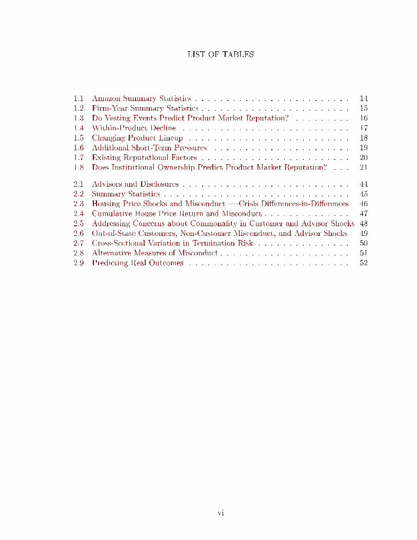
1.1 Amazon Summary Statistics . . . . . . . . . . . . . . . . . . . . . . . . . 141.2 Firm-Year Summary Statistics . . . . . . . . . . . . . . . . . . . . . . . . 151.3 Do Vesting Events Predict Product Market Reputation? . . . . . . . . . 161.4 Within-Product Decline . . . . . . . . . . . . . . . . . . . . . . . . . . . 171.5 Changing Product Lineup . . . . . . . . . . . . . . . . . . . . . . . . . . 181.6 Additional Short-Term Pressures . . . . . . . . . . . . . . . . . . . . . . 191.7 Existing Reputational Factors . . . . . . . . . . . . . . . . . . . . . . . . 201.8 Does Institutional Ownership Predict Product Market Reputation? . . . 21
2.1 Advisors and Disclosures . . . . . . . . . . . . . . . . . . . . . . . . . . . 442.2 Summary Statistics . . . . . . . . . . . . . . . . . . . . . . . . . . . . . . 452.3 Housing Price Shocks and Misconduct � Crisis Di�erences-in-Di�erences 462.4 Cumulative House Price Return and Misconduct . . . . . . . . . . . . . . 472.5 Addressing Concerns about Commonality in Customer and Advisor Shocks 482.6 Out-of-State Customers, Non-Customer Misconduct, and Advisor Shocks 492.7 Cross-Sectional Variation in Termination Risk . . . . . . . . . . . . . . . 502.8 Alternative Measures of Misconduct . . . . . . . . . . . . . . . . . . . . . 512.9 Predicting Real Outcomes . . . . . . . . . . . . . . . . . . . . . . . . . . 52
vi

LIST OF FIGURES
1.1 Number of Reviews Posted on Amazon.com in Selected Categories . . . . 22
2.1 Real Estate Price Shocks by Year . . . . . . . . . . . . . . . . . . . . . . 532.2 Crisis Price Changes in Metro Atlanta . . . . . . . . . . . . . . . . . . . 542.3 Misconduct by Ventile of Annual House Price Changes . . . . . . . . . . 552.4 Misconduct Timing around Real Estate Shocks . . . . . . . . . . . . . . 562.5 Coe�cient of Pseudo Cumulative Return in Placebo Samples . . . . . . . 57
vii

Chapter 1 Managerial Myopia and Product Market Reputation:
Evidence from Amazon.com Reviews
1.1 Introduction
The relevance of intangible assets has been steadily increasing in recent decades.In 2016, U.S. companies had over $8 trillion of intangible assets, about half of thecombined market capitalization of the S&P 500 at the time.1 While the use of intan-gible assets has been increasing, much of the current research on �rm investment stillfocuses on investment in physical assets.
Executives have long understood the value of intangible assets such as intellectualproperty, training, client relationships, and reputation. John Stuart, the CEO ofQuaker Oats in the early 20th century, once said �If this business were split up, Iwould be glad to take the brands, trademarks and goodwill and you could have allthe bricks and mortar�and I would fare better than you.� Empirical research onintangible assets, however, has historically been constrained due to the di�culty invaluing many of these assets and the relative lack of data, issues which have becomeeasier to address with modern data. Using a novel dataset of crowd-sourced customerreviews from Amazon.com, I explore an important intangible asset, product marketreputation, and show how it is impacted by managerial incentives.
Product market reputation is an amalgam of consumer opinions. It encompassesfactors such as quality, customer service, and corporate social responsibility, and itplays an important role in the decision making process of consumers. For example,customers are willing to pay higher prices and are more loyal to the �rm when the�rm has a high reputation.2 Technology consumers who have a preference for theApple ecosystem are typically aware they pay an �Apple premium,� but perceivedintangible factors such as reputation are usually cited as the justi�cation for payingthis premium. On the other hand, a low reputation harms the �rm. After admittingto using illegal software to cheat on emissions testing, Volkswagen experienced aconsumer exodus, and sales have still not fully recovered. Ceteris paribus, a positivereputation is a valuable asset for �rms.
Given the growth in the importance of intangible assets, an understanding of theirdeterminants leads to a better understanding of �rm behavior. In much the sameway executives decide to invest in physical capital, they may also decide to invest inintangible capital such as reputation. However, the characteristics of product marketreputation are notably di�erent than physical capital, so it may be the case thatinvestment in reputation is handled di�erently by executives. For instance, reputationis harder to value and �rms cannot resell it in the same way they can resell physicalcapital. It is also more di�cult for �rms to use intangible capital as collateral inlending arrangements.
1https://www.wsj.com/articles/accountings-21st-century-challenge-how-to-value-intangible-assets-1458605126
2See, e.g., Larkin (2013) and Melnik and Alm (2002)
1

In this paper I study the impact of CEO short-term incentives on product marketreputation. Speci�cally, using multiple measures of short-termism, or myopia, I �ndthat the product market reputation of a �rm is negatively impacted in the yearsfollowing CEO short-term incentive shocks. In my primary tests I use the plausiblyexogenous vesting of stock and options grants to the CEO as shocks to the incentivestructure. These vesting schedules are typically set up years in advance and aretherefore unlikely to be related to contemporaneous product market conditions. Yetthese vesting events create distortions in the incentive structure faced by managementsince they are usually accompanied by large amounts of insider selling (Edmans, Fang,and Lewellen, 2017). Executives even admit to a surprising degree that they arewilling to sacri�ce positive NPV projects when they have concerns about the near-term stock price (Graham, Harvey, and Rajgopal, 2005). I �nd that when stock veststo the CEO, the product market reputation, as measured by the average number ofstars on Amazon.com, declines by approximately 10% in the subsequent year.
A variety of mechanisms exist through which management can a�ect reputationin the product market. They may change product quality directly by adjusting theinputs used in the manufacturing process (e.g., substituting a metal component for aplastic one). Relatedly, they might also change the customer experience by increas-ing or decreasing the amount of support they provide for their products followingpurchases (e.g., outsourcing a call center). In additional tests, I incorporate product�xed e�ects to show that the myopic incentive shocks cause within-product declinesin reputation, consistent with a cost cutting mechanism.
Another potential mechanism through which reputation might be a�ected relatesto the product market composition. Firms choose when to release new products andwhen to retire old products, and the release of a new product to the market is apotentially risky event. If the product is well-received it obviously bodes well for thecompany, but a poorly received product can result in lower sales and lower reputation.A CEO that faces short-term stock price incentives could become more risk averseand delay the release of new products, reducing the rate of product releases in theevent year. Indeed I �nd that in years in which the CEO has a vesting event the�rm is more likely to reduce the rate at which they introduce new products, causinga reduction in the number of total products o�ered by the �rm.
While �rm reputation in the product market has been explored theoretically fordecades, only recently has the data allowed empirical investigation. Fortunately, therise in online shopping, and more speci�cally the availability of crowd-sourced cus-tomer reviews, now makes empirical measurement of widespread customer perceptionsmore feasible. I create the measure of product market reputation using a large sampleof user-submitted product reviews on Amazon.com, a large online retailer. In addi-tion to information on product identi�ers, the review submission date, the customerrating of the product (out of �ve stars), and the text of the review, I also collectthe brand and �rm information from each product's Amazon page. This allows meto match products to companies. This process yields information on approximately400,000 products,3 for which approximately 4.3 million reviews were written.
3A product is de�ned as a unique Amazon Standard Identi�cation Number (ASIN).
2

The Amazon.com data is particularly well-suited for this setting since productsremain on the site even after they are discontinued, thus avoiding survivorship bias.I am also able to observe reviews that were designated as Helpful by the other cus-tomers. I limit my analysis to these Helpful reviews in robustness tests, and myresults hold: a short-term incentive shock causes product market reputation to de-cline among the most helpful consumers.
As an alternative methodology, I use the �rm's ownership composition as a proxyfor the degree of short-termism. Previous work has shown that �rms with Transient(i.e., short-term) owners are on average more preoccupied with near-term results,while �rms with Dedicated (long-term) owners are not (Bushee, 2001). These supple-mentary results are consistent with the primary �ndings: �rms with CEOs who haveimmediate concerns about the stock price experience a decline in product marketreputation.
I then investigate whether there is a di�erential e�ect across existing incentivestructures. CEOs that are closer to retirement may have less of an incentive to careabout long-run �rm value, which in turn could mean that they are more likely to bea�ected by these incentive shocks. A similar e�ect may exist for highly levered �rms.Matsa (2011) shows that CEOs of highly levered supermarket �rms, with near-termcash �ow concerns for debt service, reduce quality to conserve cash. Consistent withthese hypotheses, I �nd that the negative reputational shock in the product marketis largest for �rms with CEOs nearing retirement and �rms with relatively higherleverage.
The reputational e�ect may also vary across other reputational factors. If invest-ment in reputation faces diminishing marginal returns, then the shock to short-termincentives should have more severe consequences for �rms who already have a lowreputation. This e�ect would be consistent with the �ndings of Larkin (2013) if rep-utation begets loyalty. She shows that higher brand loyalty is associated with a moreinelastic demand curve on the part of the consumers, which in turn allows the �rmto support more leverage and maintain less cash since the cost of �nancial distress islower due to lower cash �ow volatility. However, if reputation, unlike physical capital,is a fragile asset, then short-term decisions could result in more severe reputationalconsequences for �rms with high reputation.
My results are consistent with the �rst hypothesis. Firms with low reputation aremore likely to experience further reductions in product market reputation followingvesting events. This hypothesis is also supported by subsequent results that show thee�ect is mitigated when �rms spend more on advertising. Higher advertising expensescould support the inelastic demand discussed by Larkin (2013) and safeguard the �rmagainst these reputational consequences. The results also lend support to the notionof diminishing marginal returns to investment in intangible capital.
I contribute to the literature in a number of ways. First, I build and use anovel dataset that allows me to measure product market reputation, an importantintangible asset. Prior work has examined consequences of reputation. Using a sampleof corporate donations, Lev, Petrovits, and Radhakrishnan (2010) �nd that when�rms are seen as philanthropic it positively predicts sales growth, particularly for�rms whose primary customers are individuals and not other �rms. Their results
3
are consistent with the �ndings of Melnik and Alm (2002) who show that vendorswith a higher reputation are able to sell an identical product for a higher price.Gerken, Starks, and Yates (2018) show that mutual fund customers are more likelyto purchase a fund from the same family when they have had a positive experiencewith the family in the past, consistent with the bene�ts to positive reputation.4 Whilethis strand of research focuses on the consequences of reputation, I instead contributeto the literature by helping to explain how reputation is a�ected and how it can bemanaged.
I also contribute to the literature on executive compensation. It is importantto understand how compensation contracts interact with reputation in the productmarket if we are to have a better understanding of the compensation arrangements.When the incentives of the manager are not aligned with the shareholders, the man-ager may make decisions for short-term personal gain at the expense of long-termshareholder value (see Jensen and Meckling, 1976; Narayanan, 1985). While researchhas documented the impact of myopia on physical investment (Edmans, Fang, andLewellen, 2017; Moore, 2018), mergers and acquisitions (Gaspar, Massa, and Matos,2005), and earnings forecasts (Ajinkya, Bhojraj, and Sengupta, 2005), I am the �rstto my knowledge to document how CEO incentive structures relate to reputationamong consumers.
Reviews from customers o�er unique and informative data about the �rm thatthe market cannot �nd in �nancial statements, news articles, or management guid-ance. Though each individual review may not convey anything material, in aggregate,research has demonstrated the value of these crowdsourced measures. Giles (2005)examines the error rate in Wikipedia entries, a crowd-sourced knowledge base, andcompares it to the error rate in the Encyclopedia Britannica. Despite the potentialfor contribution by uneducated sources, he �nds the Wikipedia error rate to be almostidentical to the error rate of Encyclopedia Britannica. A similar relation has beenshown with earnings forecasts. Jame, Johnston, Markov, and Wolfe (2016) �nd thatcrowdsourced earnings estimates provide incremental value and can be used in tan-dem with other more traditional information to better forecast a company's earnings.This provides additional support to the hypothesis that customer reviews provide aunique and important insight into the operation of the company.
In one of the �rst papers to use Amazon.com reviews, McAuley and Leskovec(2013) use the reviews data to improve recommender system algorithms. Huang(2018) instead connects the data to stock returns and �nds that abnormal changes toreviews predict stock returns, earnings surprises, and revenue surprises. While Huang(2018) highlights another outcome of this measure, I contribute by studying factorsthat a�ect reputation among consumers.
I also contribute to the growing discussion in the literature on product markets.Sheen (2014) uses data on product quality from Consumer Reports to show that,following a merger, the quality of products between the two companies converges
4Related work examines other types of intangible assets. For example, Cli�ord and Gerken (2018)�nd that the advisor-client relationship in the market for �nancial advice is an important intangibleasset that signi�cantly impacts advisor behavior when ownership of the asset is transmitted fromemployer to employee.
4

and the price falls relative to competitors. Cavallo (2018) examines the growth of theonline product market and its macroeconomic implications. I instead study �rm-levelchanges to better understand the microeconomic implications.
Lastly, I contribute to the literature that explores the consequences of varyingownership structures. Bushee (1998) �nds that �rms with high Dedicated institutionalownership (owners with a long time horizon and low portfolio diversity) are morefocused on the long-term and are less likely to cut R&D in order to reverse an earningsdecline. The opposite is true for Transient ownership (owners with a short timehorizon and high portfolio diversity). Similarly, long-term institutional ownershiphas been shown to predict �rm pro�tability and stock market performance (Cella,2009; Cli�ord, 2008). Consistent with this literature, I �nd the investment horizonof institutional owners predicts future changes in product market reputation.
1.2 Data
1.2.1 Amazon Data
My measure of product market reputation comes from customer reviews posted onAmazon.com, one of the largest retailers in the world.5 Individual shoppers who usethe Amazon site are able to leave feedback about their experiences with products.This feedback usually consists of a small amount of text and a rating, or numberof stars out of �ve they assign the product. Speci�cally, each observation in mydata contains the Amazon Standard Identi�cation Number (ASIN) which uniquelyidenti�es the product, a user identi�er, the text of the written review, the number ofstars (out of �ve) that the user assigned to the product, the date and time the reviewwas published, and Helpful votes. When a person publishes a review on the platformother users are then able to upvote the review or downvote the review.6
I use reviews from 20 of the Amazon product categories: Arts, Automotive, Baby,Beauty, Cell Phones and Accessories, Clothing and Accessories, Electronics, GourmetFoods, Health, Home and Kitchen, Industrial and Scienti�c, Musical Instruments,O�ce Products, Patio, Pet Supplies, Shoes, Sports and Outdoors, Tools and HomeImprovement, Toys and Games, and Watches. I speci�cally avoid using reviews fromthe Music, Movies, and Video categories because of the di�cult nature of disentan-gling the reputation of the artist from the reputation of the company selling theproduct.
Since not all reviews convey new or especially valuable information, many of mytests limit the measure of reputation to only Helpful reviews. I use Helpful reviews inmuch of my analysis because of the noise that can arise from other reviews. Shoppersat Amazon.com will occasionally notice reviews that are either unhelpful, uninformed,fake, or simply posted in the wrong place.7 Illegitimate reviews are a minor concern
5The product reviews are similar to those used in McAuley and Leskovec (2013) and Huang(2018).
6Since the time of data collection Amazon has changed this process to only allow upvotes.7There have been companies that have emerged as posters of fake reviews for sellers (e.g.,
www.buyamazonreviews.com). The sellers that purchase these reviews though are smaller and
5

considering Amazon's aggressive legal pursuit of those who write fake reviews.8 Eventhough this noise a�ects only a small subsample of the reviews, I use Helpful ratingsas a robustness.
Chen, Dhanasobhon, and Smith (2008) study reviews on Amazon.com and �ndthat helpful reviews in�uence the purchasing decisions of consumers more than otherreviews. Using helpful reviews then provides me with a more precise measure, thoughthe cost of using the measure is a reduction of power in the tests.
For each ASIN, I scrape the Amazon site using a Python script for the nameof either the �rm that sells the product or the brand that is associated with theproduct. The initial dataset consists of approximately 4.3 million reviews writtenon about 400,000 products from 1999 to 2012.9 Though the data spans more thana decade, most of the observations are concentrated in the second half of the timeseries, representing the rise in popularity of the site.
I am unable to collect company information for about 3.5% of the products becausethey do not have a functioning web page, and only 1.8% of the products do not havecompany or brand information listed on the page. Though a small portion of theproducts do not have a functioning web page, survivorship bias is a minor concernsince the vast majority of discontinued products remain on the Amazon site and canbe referenced at any time.
An example observation is given in Appendix A. At the top of the product de-scription, just below the product name, there is a byline with the name of the pro-ducer/brand. In this example observation the product is the iPod Classic, and Appleis listed as the maker of the product. At the time, over 3,000 reviews had been writtenfor this iPod, with an average review of about 4.5 stars over the life of the product.The average rating displayed on the Amazon Website is a proprietary weighted aver-age of all reviews of the product, with weight given to more recent and more helpfulreviews. In order to test within-�rm variation in product market reputation, I buildan annual measure of reputation using only the reviews written in the year.
Below the product description is an example review of the product. Alex (thereviewer) gives the product �ve stars because of the impressive storage space and thereliability relative to other products. Above Alex's star rating there is also a line thatsays 1,651 people out of 1,696 voted the review as helpful.
For many products the name of the �rm is not listed on the byline. Instead itcontains either a subsidiary or a brand (e.g., Gillette razors are manufactured andsold by the company Proctor & Gamble). For these observations I use a combinationof LexisNexis and Google searches to identify the parent company. I do this fora majority of the reviews with brand and subsidiary information instead of �rminformation.
usually private companies. Since my analysis focuses on larger public companies this does notpose an issue.
8http://www.wsj.com/articles/amazon-sues-sellers-for-o�ering-fake-goods-on-its-site-1479243852
9I drop Amazon.com, the company, from my sample since it has been shown that Amazonmanipulates its product market positions in relation to products from competitors on the site (Zhuand Liu, 2018).
6

Figure 1.1 plots the number of reviews posted in the Amazon.com markets throughtime. The number of reviews posted on Amazon exploded throughout the decadeending in 2007, before plateauing at about 50,000 reviews each year. The dark bluebars represent the total number of reviews posted each year. The lighter beige barsrepresent the number of reviews that are designated as Helpful each year. In orderfor a review to be designated as Helpful at least 50 percent of the voters must classifyit as such. It is important to note here that the decline in helpful reviews after 2007is mechanical and not related to changing review quality through time. A reviewwritten in 2007 had years to collect votes, whereas a review written in 2012 only hadmonths to collect user votes.
I then match the product reviews data with data from the Center for Researchon Security Prices (CRSP) and Compustat using company names. Prior to the namematch I clean the names by dropping punctuation (e.g., �.�, �-�, �&�) and certain words(e.g., �corporation�, �incorporated�). I only keep observations that match perfectlyon these cleaned names.
Table 1.1 presents summary statistics on the Amazon data. Panel A presentsinformation on the products in the sample, and Panel B presents information onthe �rms in the sample. The initial sample covers approximately 400,000 products.However, many of the products are sold by private companies, and many observationsdo not survive the perfect name match. I also require that the �rm be included inthe ISS Incentive Lab data which contains information on executive compensation.The ISS Incentive Lab data covers the S&P 500 as well as a �signi�cant portion ofthe S&P 400�. After imposing these �lters the dataset covers approximately 12,000products from 90 companies from 1999 to 2012. The mean product has an averagerating of 3.95 stars out of �ve and has about 26 reviews (half of which are Helpful).The typical product has a lifetime on the site of �ve years.10
In Panel B, the median �rm has 94 products, introduces 3.7 products each year,and drops 2.4 products each year. The typical �rm also has over 200 reviews writtenabout its products and has an average rating of just under 4 stars. These variablesare highly skewed.
The Amazon dataset of reviews was originally scraped in 201311, so any productsthat were introduced on Amazon.com and then subsequently removed prior to 2013would not be in my sample and could potentially bias my results. There are tworeasons this concern is signi�cantly lessened. First, I incorporate tests which includeproduct �xed e�ects, which limit my analysis to within-product reputation responsesto myopia.
Second, Amazon tends to leave products on its site even when they are no longersold. In the data there are many instances of unsuccessful products that were onlysold on Amazon for a short period of time. Though they would not be include in mytests, examples can be found of products that received a single review but remain onthe Amazon site for years. I do, however, �nd few instances of product removal. But
10I use the year of the �rst review as the year the product was introduced, and I consider aproduct discontinued when it no longer receives ratings.
11For more information about the scraping process and original use of the data in a recommendersystems setting, see McAuley and Leskovec (2013)
7
even if these cases were widespread, it would bias my estimates downward. If myopiaa�ects reputation in a signi�cant enough way to cause the product to drop out of mysample then my estimates on the treatment e�ect would be too low.
1.2.2 Equity Vesting Data
My primary measure of changes to the CEO incentive structure is their vesting ofstock and options. As part of the compensation plan a CEO will frequently beawarded equity and option grants that vest at regular intervals. Many times thevesting payment will only take place if certain accounting goals have been met. Theseperformance-based grants are frequently intricate and elaborate. For the sake ofsimplicity I omit these types of payments from my analysis. I instead focus on time-based grants since these contracts are typically awarded years in advance and are notbased on any performance criteria.
Within time-based plans, grants can vest with either a cli� schedule or a ratableschedule. Ratable schedules pay a portion of the grant on a recurring basis (typicallyannually) while cli� schedules pay a lump sum on the vesting date. I limit my analysisto the most plausibly exogenous subset of vesting payments: time-based grants witha cli� schedule. I also require that these grants be awarded at least a year in advanceof the vesting date. Many of these grants vest 3-5 years after the award date.
Previous work has already used similar measures as a proxy for the CEO's short-term concern for the stock price. CEOs typically sell a large amount of equity inyears in which they receive vesting payments. It is this large degree of selling thatcreates the incentive to focus on the short-term stock price. Moore (2018) �nds that�rms are more likely to repurchase stock if the CEO has vesting equity in the period,and Edmans et al. (2017) use similar vesting data to show that the rate of investmentin R&D and CAPEX is reduced when CEO equity vests.
I create three vesting event variables to measure shocks to short-term incentives.Any Vesting Event (CEO) is set to 1 in any year in which the �rm's CEO has eithera stock vesting event or an option vesting event that is time-based with a cli� vestingschedule. I then decompose this measure into its two components: Any Stock Vesting(CEO) and Any Option Vesting (CEO). I make similar variables for vesting eventsfor any of the executives at the �rm.12 Panel A of Table 1.2 reports the percent of�rm-years a�ected by each type of vesting event. In my sample approximately onefourth of �rm-years have a CEO vesting event, 17% have a stock vesting event, and11% have an option vesting event. While some form of vesting is likely occurringevery year for large companies, the frequency of these vesting events is much lowersince I focus on the events that are the most plausibly exogenous.
1.2.3 Institutional Ownership Classi�cation and Controls
As an alternative measure of short-termism I use institutional ownership as catego-rized by Bushee (2001). He examines the portfolio diversity as well as the portfolio
12In untabulated results I use a measure that includes awards for all executives. The inferencesremain the same, though the magnitude of the e�ect is approximately two thirds the size.
8

turnover of institutions to identify transient owners (high diversity, high turnover),dedicated owners (low diversity, low turnover), and quasi indexers (high diversity, lowturnover). I obtain these classi�cations from his website and merge them into theThompson Reuters 13F holdings data to build a �rm-year measure of each type ofowner. Panel B of Table 1.2 reports summary statistics on the ownership variables.In the �nal sample, the average �rm-year has just over 50% of its shares owned byQuasi Indexers, approximately 15% owned by Transient institutions, and under 4%owned by Dedicated institutions.
From CRSP, I use data on returns, prices, volume, and shares outstanding. I alsomerge with Compustat to get data on assets, liabilities, advertising expense, cash,sales, R&D, and book value per share. Summary statistics for control variables arealso reported in Table 1.2.
Following Sheen (2014), I include LN(Market Cap), Leverage, R&D, and OperatingMargin as controls in my analysis. I also use Book-to-Market and 12-month Return.LN(Market Cap) is the natural log of price times shares outstanding. Leverage istotal liabilities divided by total assets. R&D is research and development expensesscaled by the previous year's sales. Operating Margin is operating income beforedepreciation scaled by the previous year's sales. Book-to-Market is the book valueper share divided by the price per share. 12-month Return is the return on thecompany's stock over the prior 12 months.
For the interacted tests I also include Bad Reputation which is an indicator equalto 1 if the �rm is in the lowest quartile of reputation for the year as measured byAmazon.com reviews, High Leverage which is an indicator variable equal to 1 if the�rm is above the median leverage ratio for the year, Old CEO which is an indicatorvariable equal to 1 if the CEO is over 50 years of age, and High Advertising whichis an indicator variable equal to 1 if the �rm is in the top quartile of advertisingexpenses.
1.3 Identi�cation Strategy
In order to test the causal e�ect of myopia on product market reputation, I use stockand option vesting events. The timing of these vesting events has been shown to beplausibly exogenous to contemporanous factors since they are usually set up yearsin advance. I use the subset of events that is most exogenous as a parsimoniousindicator variable. Many of the grants awarded to CEOs are based on performancemeasures, but some are strictly time-based grants that vest according to a predeter-mined schedule. I restrict my sample to time-based grants.
Within time-based grants, awards can vest with either a cli� schedule or a ratableschedule. Since cli� schedules have the largest portion of the award further into thefuture, the future payments are arguably more exogenous to the �rm conditions atthe time of vesting. In order for an endogeneity problem to exist, the compensa-tion committee would have to be able to accurately and systematically forecast �rmconditions and the reputational environment years in the future. This is unlikely.
9

1.3.1 Panel Speci�cations
My primary dependent variable is one-year ahead product market reputation. Asrobustness checks I also use two-years ahead reputation and a reputation measurebuilt using only Helpful reviews. I use a forward looking dependent variable sinceSheen (2014) �nds that following a merger the quality of products between the twocompanies converges, but this convergence takes about two to three years to mate-rialize. Changes made to the product lineup cannot be immediately re�ected in theproduct market since changes take time to make their way through the manufactur-ing process. However, this change would occur more rapidly when a �rm is not alsoconcerned about combining the resources of another company.
The model I formally test is:
Reputationi,j,t+1 = β0 + β1Vesting Eventi,t + γXi,t + θi + φt + εi,t (1.1)
where i indexes the �rm, j indexes the product, t indexes the year, Xi,t is a vector ofcontrol variables, θi represents the time-invariant �rm �xed e�ect, and φt is the year�xed e�ect that accounts for annual factors that could impact all observations in ayear. Reputation is measured as the average number of stars (out of 5) assigned to thatproduct in the subsequent year. In other speci�cations I decompose Vesting Eventinto its stock and option components, and in later tests I replace the Vesting Eventindicator variable with varying measures of institutional ownership types. Standarderrors are clustered by product in order to address the potentially correlated errorterms within the groups.13
In my second set of tests I attempt to understand the mechanism through whichreputation is a�ected. A �rm could respond by changing the existing products orchanging the product lineup by increasing/decreasing the number of products theyintroduce/drop each year. In order to test the �rst hypothesis I rerun Equation (1.1)including product �xed e�ects (which subsume the �rm �xed e�ect).
In order to determine whether the product lineup is changing, I employ a �rm-yearpanel and estimate the following model:
∆Characteristici,t = β0 + β1Vesting Eventi,t + γXi,t + θi + εi,t (1.2)
where i indexes the �rm, t indexes the year, Xi,t is a vector of control variables,and θi represents the time-invariant �rm �xed e�ect. Characteristici,t is either Num-ber of Products, Number of New Products, or Number of Dropped Products dependingon the speci�cation. In some speci�cations I again decompose Vesting Event intoits stock and option components. Standard errors are clustered by �rm in order toaddress the potentially correlated error terms within the groups. Given that the de-pendent variable measures the change in the characteristic and that the model uses�rm �xed e�ects, the β1 estimate measures how the event impacts the rate of changeof the characteristic.
My �nal set of tests explore the di�erential e�ect that myopia has across severalmeasures: High Leverage, Old CEO, High Advertising, and Bad Reputation. I use
13See Bertrand, Du�o, and Mullainathan (2004) and Petersen (2009).
10
the exogenous speci�cation of Equation (1.1), but include estimates on the interactedcoe�cients as well.
1.4 Empirical Analysis
1.4.1 Main Results
My �rst set of tests, using the vesting events as exogenous shocks to myopic incen-tives, are presented in Table 1.3. In the �rst two speci�cations the outcome variableof interest is product market reputation in the subsequent year. The next two spec-i�cations examine the e�ect two years ahead, and the �nal two limit the measureof reputation to only include Helpful reviews. Odd numbered speci�cations use AnyVesting Event as the shock to myopia, while the even numbered speci�cations splitthe indicator into its stock and option components. As stated in the discussion ofEquation (1.1), �rm and year �xed e�ects are included, and standard errors, clusteredby product, are reported in parentheses.
Results are consistent across all speci�cations.14 The estimate on Any VestingEvent is negative and statistically signi�cant at the one percent level in all threespeci�cations. The magnitude of the Stock Vesting estimate is slightly larger (thoughthe di�erence is not signi�cantly di�erent from zero) and also statistically signi�cant.The estimates for the coe�cients on Option Vesting are indistinguishable from zero.These results are consistent with myopia negatively impacting reputation, and theyare also consistent with Edmans et al. (2017) who �nd that the reduction in physicalinvestment is concentrated primarily in the stock vesting.15
The lack of signi�cance on the Option Vesting is not surprising. Many of theseoption vesting events grant the CEO an option that is out of the money. In theseinstances, the CEO does not experience a myopic shock.
The magnitudes on the estimates are also economically meaningful. A stockvesting event to the CEO is associated with an average decline of 0.10 stars in thenext year's average rating, or 10% of the unconditional average interquartile range.
1.4.2 Mechanism
Table 1.4 repeats the analysis using product �xed e�ects instead of �rm �xed e�ectsto test the product deterioration hypothesis. The quantitative results are similar,but the interpretation is slightly di�erent. The tests provide evidence that followingshort-term incentive shocks, individual products deteriorate. Multiple explanationsexist for this deterioration. Two potential explanations are that the manufacturingprocess may be altered, or perhaps the �rm reduced customer service for the productfollowing sales. Either way, the reputation of the product among consumers declines.
Table 1.5 estimates Equation (1.2). Again, even speci�cations decompose thevesting event variable into its stock and option components. Speci�cations (3) and (4)
14See Internet Appendix Table IA1.1 for control variable details.15Internet Appendix Table IA1.2 repeats this analysis using all executives instead of just the
CEO.
11

use two-year ahead reputation as the dependent variable, and speci�cations (5) and(6) limit the reputation measure to only include Helpful reviews. In all speci�cationsstandard errors are clustered at the �rm level and reported in parentheses.
The results are consistent with the risk aversion story. Firms with CEOs who areshocked with a short-term incentive change reduce the number of products they o�er.Speci�cations (3) and (4) show that this reduction in the number of products is dueto a reduction in the rate at which new products are released. Since releasing newproducts is a risky activity, CEOs appear to be reducing their risk-taking to protectthe stock price in vesting years.
1.4.3 Cross-Sectional Variation in Myopia and Reputation
The next set of tests repeats speci�cations (1) and (2) from Table 1.3 with interactedindicator variables. Table 1.6 reports results from testing whether or not there is adi�erential e�ect across �rms with existing short-term pressures. Table 1.7 reports re-sults from testing whether or not there is a di�erential e�ect across other reputationalfactors.
CEOs that are older and closer to retirement have less of an incentive to careabout the long-run �rm prospects, which in turn could mean that they are morelikely to be a�ected by these incentive shocks. Similarly, Matsa (2011) shows thatCEOs of highly levered supermarket �rms, with a near-term concern about cash �owfor debt service, reduce quality to conserve cash. Consistent with these hypotheses,I �nd that the negative reputational shock in the product market is largest for �rmswith an older CEO and �rms with high leverage.
Consistent with the notion of diminishing marginal returns to investment in rep-utation, I �nd that the shock to short-term incentives has more severe consequencesfor �rms who already have a bad reputation. This is consistent with the �ndings ofLarkin (2013) that higher brand loyalty is associated with a more inelastic demandcurve on the part of the consumers. Firms with a high reputation are able to �weathera storm� better than poorly-perceived �rms. This hypothesis is also supported bythe results that show the e�ect is mitigated when �rms spend more on advertising.Higher advertising expenses appear to safeguard the �rm against these reputationalconsequences.
1.4.4 Institutional Ownership
In the last set of tests I use an alternative empirical strategy, looking instead at in-stitutional ownership and its e�ect on product market reputation. Several papershave used institutional ownership as a measure of �rm myopia.16 I decompose insti-tutional ownership into separate components since the time horizon of the owner hasbeen shown to a�ect �rm behavior. Bushee (2001) classi�es institutional owners intoTransient, Dedicated, and Quasi Indexers. These classi�cation are available on hisWebsite. Table 1.8 presents the results.
16See, e.g., Cella (2009), Bushee (1998), Derrien, Kecskés, and Thesmar (2013).
12

The two measures of interest are Dedicated Ownership and Transient Ownership.Dedicated Ownership measures the fraction of shares outstanding that are ownedby institutional owners with long investing horizons and low levels of diversi�cation,while Transient Ownership measures the fraction of shares outstanding that are ownedby institutional owners with short investing horizons and high levels of diversi�cation.Investors classi�ed as Quasi Indexers have long investing horizons and high levels ofdiversi�cation.
Increases to Dedicated Ownership predict higher product market reputation. Theopposite result holds for Transient Ownership. Limiting the measure of reputation toHelpful reviews, the interpretation and inferences hold. When a �rm has an increasein owners with a short-term focus its product market reputation declines.
The institutional ownership speci�cations do face an endogeneity problem, how-ever. It is possible that dedicated institutions are particularly good at targeting �rmswith better future prospects and that institutions are not actually a�ecting myopiaat all. However, Edmans (2009) argues that simply the threat of exit by these largeinstitutions causes management to focus on the long-term. If management decidesto act myopically then these institutions will �vote with their feet� and add sellingpressure to the stock, thus reducing the incentive to act myopically. At a minimumthese tests provide additional evidence in support of the conclusions reached in theprimary analysis.
1.5 Conclusion
In this paper I examine a �rm's product market consequences when its managementhas myopic, or short-term, incentives. Speci�cally, I �nd that the �rm's productmarket reputation is negatively impacted when the �rm's management has short-term vesting incentives in the current year. In my primary tests I use the exogenousvesting of options and stock grants to the �rm's CEO. These vesting events are set upyears in advance and are therefore unlikely to be related to current product marketoutcomes. I �nd evidence that this decline is driven by a deteriorating of existingproducts (cost cutting) as well as changes to the �rm's product lineup (risk aversion).
I �nd that the negative reputational shock in the product market is largest for�rms with an older CEO and �rms with high leverage. Consistent with the notionof diminishing marginal returns to investment in reputation, I �nd that the shock toshort-term incentives has more severe consequences for �rms who already have a badreputation, though higher advertising expenses appear to safeguard the �rm againstthese reputational consequences.
I use the composition of the �rm's ownership as an alternative empirical method-ology to estimate the degree of short-term focus. Previous work has shown that�rms with transient owners are on average more preoccupied with near-term results,while �rms with more dedicated ownership are not. These results con�rm the initial�ndings that a �rm's myopic focus negatively impacts its reputation in the productmarket.
13

Table 1.1: Amazon Summary Statistics
This table presents summary statistics on Amazon variables. Product variables arein Panel A while �rm variables are in Panel B. Average Rating measures the averagenumber of stars (out of �ve) assigned by users to either the product or the �rm.Average Rating from Helpful uses only reviews that were classi�ed as Helpful byAmazon voters. Also included are the number of reviews, number of helpful reviews,number of products, average product lifespan, and the average number of productsintroduced and dropped each year by the typical �rm.
Panel A: Product variablesMean Q1 Median Q3 N
Average Rating 3.952 3.500 4.091 4.500 12,309Average Rating from Helpful 3.951 3.500 4.111 4.714 11,340Reviews 26.07 3 7 20 12,309Helpful Reviews 13.97 2 4 11 12,309Product Life (years) 5.540 3 5 7 12,309
Panel B: Firm variablesMean Q1 Median Q3 N
Products 869.2 15 94 748 90Yearly New Products 23.21 0.895 3.734 21.96 90Yearly Dropped Products 16.94 0.429 2.417 16.52 90Average Rating 3.904 3.667 4.008 4.199 90Average Rating from Helpful 3.856 3.580 3.948 4.200 90Reviews 3,745 24 220.5 4,203 90Helpful Reviews 2,007 9 124.5 2,137 90
14

Table 1.2: Firm-Year Summary Statistics
This table presents summary statistics on the measures of short-term incentives aswell as other variables used in the analysis. Panel A presents the percent of �rm-yearsa�ected by vesting events as de�ned in the paper. Any Vesting Event (CEO) is setto 1 in a year where a time-based grant with a cli� schedule vests to the CEO. Thegrant must be set up at least one year in advance. Any Vesting Event (All Execs) isde�ned similarly, but includes vesting to all executives. The measures are also splitinto their stock and option components. The mean, median, 25th percentile, and 75th
percentile, along with the number of associated �rm-years, are reported in Panel Bfor other variables used in the analysis. See the data section for detailed variablede�nitions.
Panel A: Vesting events%
Any Vesting Event (CEO) 24.8Any Vesting Event (All Execs) 36.4Any Stock Vesting (CEO) 17.0Any Stock Vesting (All Execs) 26.4Any Option Vesting (CEO) 11.3Any Option Vesting (All Execs) 15.8
Panel B: Firm controlsMean Q1 Median Q3 N
Market Cap (millions) 30,672 2,152 5,128 19,903 698Book-to-Market 0.374 0.218 0.348 0.517 698Leverage 0.598 0.437 0.593 0.730 69812-month Return 0.122 -0.172 0.0683 0.308 698Advertising Expense 0.0410 0.00997 0.0247 0.0515 482Operating Margin 0.164 0.112 0.153 0.222 698R&D 0.0616 0.0155 0.0320 0.0868 698Short Interest Ratio 0.0384 0.0139 0.0266 0.0475 671Dedicated Ownership 0.0376 0.00001 0.00160 0.0591 620Transient Ownership 0.163 0.0886 0.139 0.213 620Quasi Index Ownership 0.518 0.413 0.532 0.639 620
15

Table 1.3: Do Vesting Events Predict Product Market Reputation?
This table presents the results from estimating Equation (1.1) and its variants. The dependent variable in columns (1) and (2)is measured as the average number of stars (out of 5) assigned to the product in the subsequent year. The second and thirdsets of speci�cations use two-year ahead product market reputation and the reputation as measured by the Helpful reviews,respectively. Any Vesting Event is an indicator variable set to 1 in any year in which the �rm's CEO has either a stock vestingevent or an option vesting event. Any Stock Vesting and Any Option Vesting decompose Any Vesting Event accordingly. Seethe data section for detailed variable de�nitions. Control variables are included in the speci�cations and de�ned in the text.Indicators for �xed e�ects are reported at the bottom of the table, and standard errors, clustered at the product level, arereported in parentheses. Asterisks represent the conventional levels of statistical signi�cance.
Reputationt+1 Reputationt+2 Helpful Reputationt+1
(1) (2) (3) (4) (5) (6)
Any Vesting Event -0.067∗∗∗ -0.071∗∗∗ -0.070∗∗∗
(0.018) (0.021) (0.017)
Stock Vesting -0.101∗∗∗ -0.114∗∗∗ -0.098∗∗∗
(0.020) (0.024) (0.020)
Option Vesting 0.022 0.035 -0.008(0.029) (0.037) (0.031)
Controls Yes Yes Yes Yes Yes YesFirm FE Yes Yes Yes Yes Yes YesYear FE Yes Yes Yes Yes Yes YesR2 0.063 0.063 0.064 0.064 0.066 0.067Observations 52,924 52,924 40,646 40,646 50,168 50,168
16

Table 1.4: Within-Product Decline
This table repeats the analysis from Table 1.3 using product �xed e�ects instead of �rm �xed e�ects. Control variables areincluded in the speci�cations and de�ned in the text. Indicators for �xed e�ects are reported beneath the panels. Standarderrors (reported in parentheses) are clustered at the product level. Asterisks represent the conventional levels of statisticalsigni�cance.
Reputationt+1 Reputationt+2 Helpful Reputationt+1
(1) (2) (3) (4) (5) (6)
Any Vesting Event -0.054*** -0.017 -0.045***(0.016) (0.018) (0.014)
Stock Vesting -0.079*** -0.038* -0.059***(0.019) (0.022) (0.016)
Option Vesting 0.031 0.030 0.014(0.027) (0.031) (0.026)
Controls Yes Yes Yes Yes Yes YesProduct FEs Yes Yes Yes Yes Yes YesYear FEs Yes Yes Yes Yes Yes YesR2 0.528 0.529 0.542 0.542 0.687 0.687Observations 50,400 50,400 38,961 38,961 48,032 48,032
17

Table 1.5: Changing Product Lineup
This table presents results from estimating variants of Equation (1.2). ∆ Products is the one-year change in the number ofproducts listed by the �rm. ∆ New Products is the change in the number of new products listed on Amazon by the companyin the year. ∆ Dropped Products is the change in the number of products that were reviewed in the previous year but not thecurrent year. Control variables are included in the speci�cations and de�ned in the text. Indicators for �xed e�ects are reportedbelow. Standard errors (reported in parentheses) are clustered at the �rm level. Asterisks represent the conventional levels ofstatistical signi�cance.
∆ Products ∆ New Products ∆ Dropped Products(1) (2) (3) (4) (5) (6)
Any Vesting Event -4.12* -1.70 0.52(2.23) (1.25) (0.72)
Stock Vesting -8.41*** -2.90** 0.77(2.53) (1.23) (0.68)
Option Vesting 2.14 0.97 0.54(3.68) (2.18) (1.77)
Controls Yes Yes Yes Yes Yes YesFirm FEs Yes Yes Yes Yes Yes YesR2 0.13 0.14 0.05 0.05 0.27 0.27Observations 732 732 647 647 647 647
18
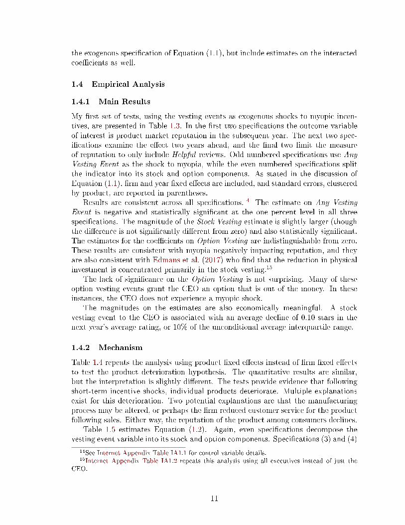
Table 1.6: Additional Short-Term Pressures
This table presents estimates from versions of speci�cations (1) and (2) from Table 1.3.The dependent variable is one-year-ahead product market reputation and is measuredas the average number of stars (out of 5) assigned to the product. Near Retirementis an indicator variable equal to 1 if the CEO is over 50 years of age. High Leverageis an indicator variable equal to 1 if the �rm is above the annual median leverageratio. Any Vesting Event is an indicator variable set to 1 in any year in whichthe �rm's CEO has either a stock vesting event or an option vesting event. AnyStock Vesting and Any Option Vesting decompose Any Vesting Event accordingly.Control variables are included in the speci�cations and de�ned in the text, thoughthey are omitted for brevity. Indicators for �xed e�ects are reported at the bottomof the table, and standard errors, clustered by product, are reported in parentheses.Asterisks represent the conventional levels of statistical signi�cance.
Reputationt+1
(1) (2) (3) (4)
Any Vesting Event -0.0296 -0.0196(0.0225) (0.0302)
Stock Vesting Event -0.0358 -0.0385(0.0283) (0.0318)
Any × Near Retirement -0.1226***(0.0383)
Stock × Near Retirement -0.1225***(0.0418)
Any × High Leverage -0.0663*(0.0340)
Stock × High Leverage -0.0952***(0.0362)
Near Retirement -0.0460* -0.0464*(0.0269) (0.0272)
High Leverage -0.0769*** -0.0781***(0.0183) (0.0182)
Controls Yes Yes Yes YesFirm FEs Yes Yes Yes YesYear FEs Yes Yes Yes YesR2 0.066 0.066 0.063 0.063Observations 37,107 37,107 52,924 52,924
19

Table 1.7: Existing Reputational Factors
This table presents estimates from versions of speci�cations (1) and (2) from Table 1.3.The dependent variable is one-year-ahead product market reputation and is measuredas the average number of stars (out of 5) assigned to the product. Low Reputation isan indicator variable equal to 1 if the �rm is in the lowest annual quartile of reputationas measured by Amazon.com reviews. High Advertising is an indicator variable equalto 1 if the �rm is in the top annual quartile of advertising expenses. Any VestingEvent is an indicator variable set to 1 in any year in which the �rm's CEO has eithera stock vesting event or an option vesting event. Any Stock Vesting and Any OptionVesting decompose Any Vesting Event accordingly. Control variables are includedin the speci�cations and de�ned in the text, though they are omitted for brevity.Indicators for �xed e�ects are reported at the bottom of the table, and standarderrors, clustered by product, are reported in parentheses. Asterisks represent theconventional levels of statistical signi�cance.
Reputationt+1
(1) (2) (3) (4)
Any Vesting Event -0.0638*** -0.0572***(0.0176) (0.0212)
Stock Vesting Event -0.0903*** -0.1003***(0.0203) (0.0244)
Any × Low Reputation -0.2379**(0.1008)
Stock × Low Reputation -0.2065**(0.1031)
Any × High Advertising 0.0822**(0.0405)
Stock × High Advertising 0.1206**(0.0498)
Low Reputation -0.2413*** -0.2420***(0.0314) (0.0312)
High Advertising 0.0575 0.0666(0.0411) (0.0407)
Controls Yes Yes Yes YesFirm FEs Yes Yes Yes YesYear FEs Yes Yes Yes YesR2 0.065 0.065 0.053 0.053Observations 52,924 52,924 46,382 46,382
20

Table 1.8: Does Institutional Ownership Predict Product Market Reputation?
This table presents estimates of the e�ect of institutional ownership on product market reputation. The dependent variablein columns (1) and (2) is measured as the average number of stars (out of 5) assigned to the product in the subsequent year.The second and third sets of speci�cations use two-year ahead product market reputation and the reputation as measured bythe Helpful reviews, respectively. Transient, Dedicated, and Quasi Indexer measure the fraction of shares outstanding thatare owned by institutional owners who have been classi�ed as such as in Bushee (2001). Control variables are included inthe speci�cations and de�ned in the text, though they are omitted for brevity. Indicators for �xed e�ects are reported at thebottom of the table, and standard errors, clustered at the product level, are reported in parentheses. Asterisks represent theconventional levels of statistical signi�cance.
Reputationt+1 Reputationt+2 Helpful Reputationt+1
(1) (2) (3) (4) (5) (6) (7) (8) (9)
Transient -0.174*** -0.017 -0.367***(0.064) (0.079) (0.069)
Dedicated 0.953*** 0.738*** 1.118***(0.123) (0.137) (0.126)
Quasi Indexer -0.262*** -0.495*** -0.099*(0.052) (0.067) (0.054)
Controls Yes Yes Yes Yes Yes Yes Yes Yes YesFirm FEs Yes Yes Yes Yes Yes Yes Yes Yes YesYear FEs Yes Yes Yes Yes Yes Yes Yes Yes YesR2 0.067 0.067 0.067 0.060 0.060 0.061 0.080 0.081 0.080Observations 79,319 79,319 79,319 61,951 61,951 61,951 75,342 75,342 75,342
21
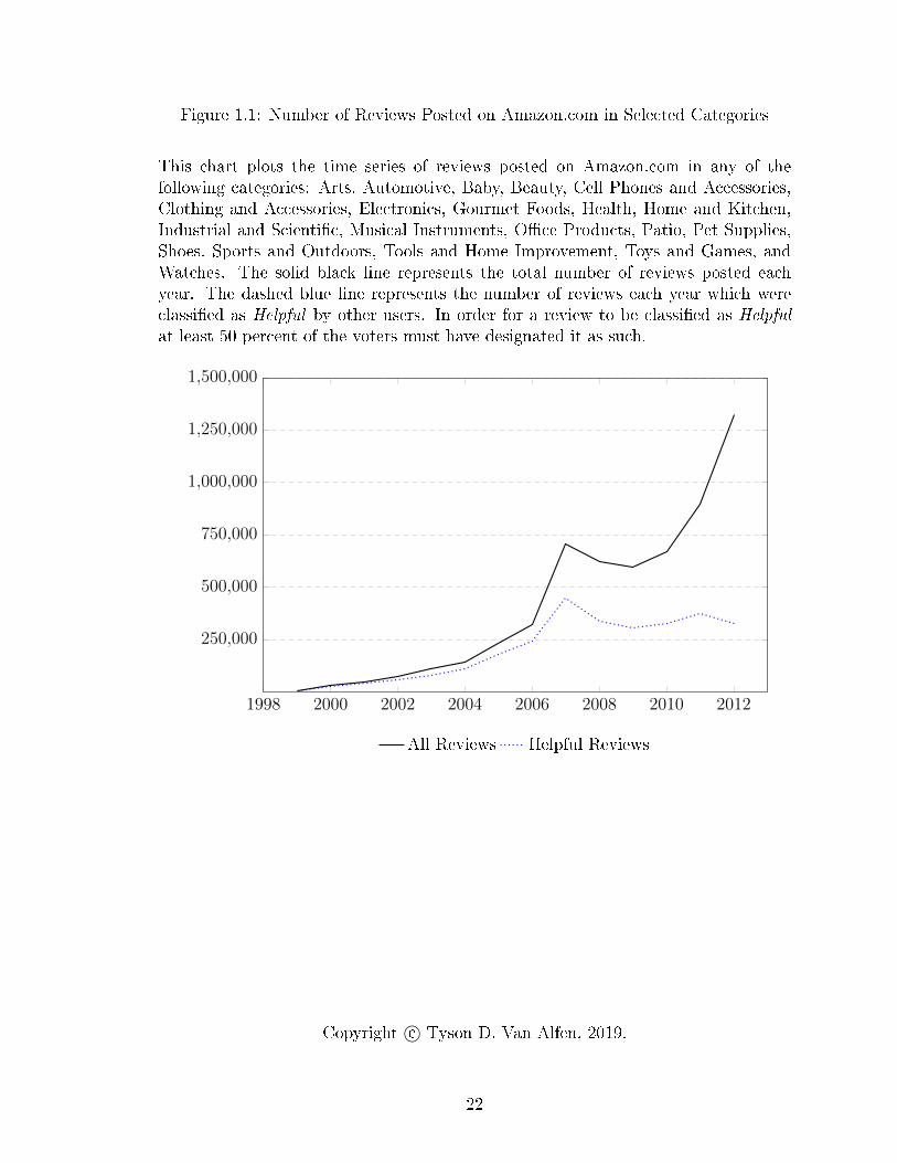
Figure 1.1: Number of Reviews Posted on Amazon.com in Selected Categories
This chart plots the time series of reviews posted on Amazon.com in any of thefollowing categories: Arts, Automotive, Baby, Beauty, Cell Phones and Accessories,Clothing and Accessories, Electronics, Gourmet Foods, Health, Home and Kitchen,Industrial and Scienti�c, Musical Instruments, O�ce Products, Patio, Pet Supplies,Shoes, Sports and Outdoors, Tools and Home Improvement, Toys and Games, andWatches. The solid black line represents the total number of reviews posted eachyear. The dashed blue line represents the number of reviews each year which wereclassi�ed as Helpful by other users. In order for a review to be classi�ed as Helpfulat least 50 percent of the voters must have designated it as such.
1998 2000 2002 2004 2006 2008 2010 2012
250,000
500,000
750,000
1,000,000
1,250,000
1,500,000
All Reviews Helpful Reviews
Copyright c© Tyson D. Van Alfen, 2019.
22

Chapter 2 Real Estate Shocks and Financial Advisor Misconduct
2.1 Introduction
Do household level �nancial shocks cause employees to commit �nancial misconduct?Anecdotal evidence has long suggested a relation between �nancial well-being anddeviant behavior. Indeed, over two thousand years ago Aristotle called poverty the�parent� of crime. More recently, in a series of interviews with professionals convictedof white collar crimes, Cressey (1971) found that �nancial pressure nearly always pre-ceded misconduct. Interpreting the observed relation between �nancial pressure andmisconduct is challenging, however, because �nancial pressure is often the result ofthe individual's own choices. For example, Cressey (1971) found that �nancial pres-sure was primarily due to gambling, alcoholism, drug use, and extravagant spending.Thus, it is unclear if negative �nancial shocks cause misconduct or if they are bothsymptoms of the same underlying personality traits or preferences.
Theory also does not provide de�nitive guidance, because the e�ect of wealthshocks on misconduct is ambiguous without strong assumptions about utility. Onthe one hand, �nancial misconduct is a risky activity; it could create illicit gains,but could result in penalties and negative career consequences.1 Under decreasingabsolute risk aversion, negative wealth shocks increase sensitivity to risk, implyingless willingness to engage in misconduct. On the other hand, Block and Heineke(1975) show that, if individuals have ethical preferences, the relation between wealthand misconduct is considerably more complicated, and the e�ect of a wealth shockdepends upon whether ethical behavior is a normal or an inferior good. Their modelfurther shows that understanding the relation between wealth and misconduct iscritical for evaluating policy responses.
Ultimately, whether �nancial pressure causes misconduct is an empirical questionthat can only be tested with exogenous wealth shocks. In this paper, we use plausiblyexogenous shocks to �nancial advisors' wealth based on housing price shocks. We usea series of �xed e�ect strategies to exploit within advisor, within ZIP code, and within�rm-year variation to identify whether household wealth shocks a�ect the propensityof �nancial advisors to engage in misconduct.
We examine the �nancial advisory industry for several reasons. First, advisorshave large e�ects on household �nancial well-being. Hung, Clancy, Dominitz, Talley,Berribi, and Suvankulov (2008) show that the majority of individual investors consultan advisor for �nancial decisions, and Foerster, Linnainmaa, Melzer, and Previtero(2017) show advisors strongly in�uence household portfolio choice. Given this keyrole in facilitating household access to �nancial markets, it is critical that householdsare able to trust their advisor with their money (Gennaioli, Shleifer, and Vishny,2015). Second, advisors are primarily compensated through commissions, which cre-
1Prior studies showing negative career consequences for �nancial misconduct include Egan,Matvos, and Seru (2018a) for �nancial advisors, Karpo�, Lee, and Martin (2008) for corporateexecutives, and Fich and Shivdasani (2007) for corporate directors.
23

ates con�icts of interest and incentives for misconduct.2 Empirical studies such asDimmock, Gerken, and Graham (2018) and Egan, Matvos, and Seru (2018a) showthat misconduct in this industry is common. A surprisingly high fraction of advisorshave a history of exploiting their clients through activities such as churning, unautho-rized trading, misrepresentation, and selling unsuitable investments. Third, the datafor this industry allow us to link misconduct to speci�c individuals within a �rm.
Our data come from detailed mandatory disclosure �lings made by �nancial ad-visors, which identify �nancial misconduct committed by speci�c advisors as well astheir employment histories (see Dimmock, Gerken, and Graham, 2018; Egan, Matvos,and Seru, 2018a,b). In addition, these mandated �lings also include the advisors'home addresses and the dates of residency. We combine the advisor addresses withZIP code level house price indexes created by Zillow and impute a purchase price andtime-series of house price returns for each advisor in the sample.3
We use house price returns as exogenous shocks to �nancial advisors' personalwealth. For our purposes, we require a shock that is both unanticipated and eco-nomically meaningful. Cheng, Raina, and Xiong (2014) analyze whether midlevelmanagers working in securitized �nance believed there was a housing bubble in 2004�2006 by examining the managers' personal home transactions; they �nd no evidencethat these individuals anticipated the housing crisis. A large literature shows thathousing price �uctuations have large, economically meaningful e�ects on consumption(see Campbell and Cocco, 2007; Carroll, Otsuka, and Slacalek, 2011; Mian, Rao, andSu�, 2013; DeFusco, 2018). Gan (2010) shows that housing shocks a�ect consumptioneven for households that do not re�nance, and argues this is consistent with changesin precautionary savings due to real estate wealth e�ects. Thus, real estate shocksappear to be both unexpected and economically meaningful.
Following other studies on risk taking by professionals around the housing cri-sis (Bernstein, McQuade, and Townsend, 2018; Pool, Sto�man, Yonker, and Zhang,2018), we estimate di�erences-in-di�erences models, in which we regress changes inan advisor's misconduct on his housing price shock during the �nancial crisis. Thesespeci�cations include �rm �xed e�ects, which control for potential confounding vari-ation among employees within a �rm (e.g., if within-�rm incentives to commit mis-conduct change during the �nancial crisis). The results show that advisors who su�erlarger housing price declines subsequently increase their commission of misconduct.For example, advisors who su�er a price decline of 10% or more increase misconductby 41% relative to advisors with smaller price declines.
We then extend the di�erences-in-di�erences results to �xed e�ect panel regres-sions using cumulative housing returns since purchase. In these tests, the unit ofobservation is advisor-year, which allows us to use housing price declines that oc-
2See Bergstresser, Chalmers, and Tufano (2009), Hackethal, Haliassos, and Jappelli (2012),Inderst and Ottaviani (2012), Mullainathan, Noeth, and Schoar (2012), Chalmers and Reuter (2015),and Hoechle, Ruenzi, Schaub, and Schmid (2018).
3In robustness tests, we show that the imputed house price returns are a highly signi�cantpredictor of actual bankruptcies �led by �nancial advisors. We also have a subsample of advisorsfor whom we have residence-speci�c Zillow valuation estimates. We �nd that the average time seriescorrelation between the residence-speci�c price changes and the ZIP code price changes is 0.803.
24

curred at any point during the 1999�2013 period. These speci�cations include ad-visor, �rm-year, and ZIP code �xed e�ects. The advisor �xed e�ects remove theadvisor's overall propensity to commit misconduct, as well as individual characteris-tics such as gender, education, and religious background. The �rm-year �xed e�ectsremove variation from the employing �rms' tolerance of misconduct or its businessmodel (even if these e�ects are time-varying). The �rm-year �xed e�ects also removeany time-series changes that a�ect all advisors, such as the overall economy. The ZIPcode �xed e�ects remove the characteristics of the area, such as demographics, localculture, state-level regulation, etc. The panel regression results are consistent withthe di�erences-in-di�erences test: advisors who su�er negative house price shocksare signi�cantly more likely to commit misconduct. Additional results show that therelation between cumulative housing returns and misconduct is non-linear and thatmisconduct is signi�cantly more sensitive to large losses on housing.
In the next set of tests, we exploit our ability to observe each advisor's cumulativehousing return since purchase. Even advisors living in the same ZIP code at thesame time can have very di�erent cumulative housing returns. For example, considertwo advisors living in the same ZIP code in 2008 but who purchased their homesat di�erent times. Although prices declined in 2008, an advisor who purchased ahome in 1986 would likely have a positive cumulative return, while an advisor whopurchased a home in 2006 would likely have a negative cumulative return. Thisvariation in cumulative returns across advisors in the same ZIP code during the sameyear allows us to include ZIP-year �xed e�ects to remove any local time-varyingconfounding variation, such as shocks to the home prices of the local customer base.In an additional test, we include branch-ZIP-year �xed e�ects. In this speci�cation,the �xed e�ects limit the comparison to advisors who live in the same ZIP code duringthe same year, and who also work at the same branch of the same �rm. Even withthese more stringent �xed e�ects, we continue to �nd that large negative cumulativereturns are associated with higher misconduct.
In our next tests, we use two alternative dependent variables based on misconductreported by non-local parties. This alleviates concerns about the commonality of thehome price shock su�ered by the advisor and the shock su�ered by local customers.First, we limit the dependent variable to include only instances of misconduct forwhich the advisor and the customer live in di�erent states. Second, we de�ne mis-conduct as either a �nalized regulatory sanction or a termination of the advisor by hisemployer (and exclude all advisor-year observations that include a customer-drivencomplaint to ensure this alternative dependent variable is distinct from the primarydependent variable). For both of the alternative dependent variables, we continue to�nd a signi�cant negative relation between cumulative returns and misconduct.
We next examine cross-sectional variation in the risk that an advisor is terminatedfor misconduct. Egan, Matvos, and Seru (2018a,b) show there is large variation in thelikelihood an advisor is terminated after committing misconduct � some �rms aremore tolerant of misconduct and women are punished more severely than men. Allelse equal, higher career risk implies a lower expected return to misconduct, reducingthe incentive to commit misconduct. Consistent with this intuition, we �nd that therelation between cumulative housing returns and misconduct is stronger for advisors
25

who are less likely to be terminated if misconduct is detected.We next explore the mechanism through which housing losses a�ect professional
misconduct. The relation could be caused by active misconduct, in which advisorsdeliberately exploit clients for �nancial gain. Alternatively, the relation could becaused by passive misconduct, in which advisors harm clients through inattentionwhen they are distracted due to �nancial distress. To test these competing mecha-nisms, we categorize misconduct as active (misrepresentation, churning, unauthorizedtrading, etc.) or passive (negligence or omission of key facts). We �nd evidence ofpassive misconduct, but more importantly we �nd highly signi�cant evidence of activemisconduct; following housing losses, advisors deliberately exploit their clients.
In additional tests, we show that the results are robust to alternative de�nitionsof misconduct. We also validate our key independent variable by showing that ourmeasure of housing price shocks accurately predicts actual bankruptcy �lings andunderwater home sales by �nancial advisors.
Our paper is related to the recent literature on misconduct by �nancial advisors.Dimmock, Gerken, and Graham (2018) show evidence of peer e�ects in misconduct;�nancial advisors are more likely to commit misconduct if they are exposed to co-workers with a history of misconduct. Egan, Matvos, and Seru (2018a) study howmisconduct a�ects the labor market for �nancial advisors and �nd that certain �rmsspecialize in misconduct while others strive to maintain clean reputations. Egan,Matvos, and Seru (2018b) study gender di�erences in the punishment for misconductand �nd that following misconduct female advisors are more likely to be terminatedand less likely to �nd new positions. Charoenwong, Kwan, and Umar (2018) showthat variation in regulatory oversight a�ects the propensity of advisors to engagein misconduct. Cli�ord and Gerken (2018) show that the assignment of propertyrights to client relationships reduces misconduct by advisors. In our paper, we showthat willingness to engage in misconduct is a pliable characteristic of the individualadvisor; advisors are more likely to commit misconduct when they are under personal�nancial pressure. Understanding such causes of �nancial misconduct is importantfor designing and implementing monitoring and regulatory systems.
Our paper is also related to several recent studies that show how personal �nancialissues a�ect professional behavior. Pool, Sto�man, Yonker, and Zhang (2018) showthat mutual fund managers who su�er negative shocks to their home's value subse-quently reduce portfolio risk and tracking error. Bernstein, McQuade, and Townsend(2018) show that workers who su�ered larger losses on their house values duringthe �nancial crisis subsequently undertook less risky and less innovative projects.Maturana and Nickerson (2018) show that when teachers declare bankruptcy, theirstudents' scores on standardized tests fall. Our paper also studies the e�ect of house-hold �nancial losses on professional behavior, but we study misconduct rather thanportfolio risk or productivity.
Our results show there are wealth e�ects in ethical behavior � a �nding that hasimplications for interpreting economic models of crime and misconduct (see Blockand Heineke, 1975). Extant empirical studies of crime and economic shocks largelyfocus on labor markets, where the key issue is how labor market shocks a�ect thesubstitution between time spent on labor versus criminal activity (see Chal�n and
26
McCrary, 2017). Relative to these studies, our setting has two unique features. First,the wealth shock is not directly related to the return on labor or on misconduct.Second, we study misconduct at work, and so the allocation of time between laborand misconduct is not a relevant issue. These features allow us to clearly identifywealth e�ects in ethical behavior, independent from the issue of time allocation.
We also document another important externality of housing price shocks. Asidefrom the direct wealth e�ects of housing price declines, several papers documentless obvious adverse consequences. Campbell, Giglio, and Pathak (2011) show thatforeclosures have spillover e�ects that reduce the value of neighboring houses. Mian,Rao, and Su� (2013) highlight the decline in consumption following the housingcrisis. We show another externality � investors su�er increased active misconductand passive mismanagement as a result of their �nancial advisors' real estate priceshocks.
2.2 Data and Sample Construction
Our �nancial advisor data come from a panel of mandatory disclosures made in FormU4 �lings. All registered representatives4 in the U.S. are required to �le and updatethese forms following any material changes. FINRA assigns each advisor a uniqueindividual permanent identi�er that allows us to track advisors even if they switchemployers. We obtain this panel through a combination of Freedom of InformationAct (FOIA) requests �led with state regulators by the authors, third-party dataobtained from a vendor (Meridian IQ), and the FINRA BrokerCheck Website.5 SeeDimmock, Gerken, and Graham (2018) and Egan, Matvos, and Seru (2018a,b) fordetailed explanations of the data and industry.
The �nancial advisor data include residential addresses for the 1999�2013 period,as well as all misconduct disclosures made during the 1999�2017 period. The sampleincludes 428,108 advisors with complete residential histories. We combine the advisordata with ZIP code level housing price data from Zillow. However, because Zillowdoes not provide the necessary data for all ZIP codes,6 our �nal sample contains329,418 advisors.
2.2.1 Financial Advisor Data
The Form U4 data includes each advisor's employment history, licenses, quali�ca-tions, and any mandated disclosures. Advisors are required to disclose certain infor-mation about customer complaints, regulatory actions, civil and criminal legal cases,terminations, and bankruptcies. Table 2.1 summarizes this disclosure information.
4�Registered representative� is the term FINRA uses for these individuals. Following the recentacademic literature, in this paper we use the term �nancial advisor. These individuals are alsocommonly referred to as brokers or �nancial planners.
5The BrokerCheck website allows investors to access a subset of the data reported in the FormU4 �lings. BrokerCheck does not report the advisors' home addresses. See https://brokercheck.finra.org/.
6Since the Zillow data is also limited to the United States we are unable to include foreignaddresses.
27

Columns (1) and (2) report the number of advisor-years with the disclosure and thepercentage, respectively. Column (3) reports the percent of advisors who make adisclosure at any time during the sample period.
Following Dimmock, Gerken, and Graham (2018), our primary measure of mis-conduct is based on validated customer complaints. Customer complaints are formalcomplaints, in which a customer demands compensation for damages caused by anadvisor's misconduct. Although some customer complaints allege negligence, mostcomplaints allege improper behavior taken to increase the advisor's compensation.Financial advisors are compensated primarily based on the amount of revenue theygenerate for their �rm (see Hung, Clancy, Dominitz, Talley, Berribi, and Suvankulov,2008), which creates strong incentives for advisors to generate trading commissionsor to sell products with high distribution fees. Theoretical models show that theseincentives encourage misconduct7 and empirical tests �nd support for the models'predictions.8
After a customer �les a complaint, it can be resolved through arbitration, settle-ment, or withdrawal. Following Dimmock, Gerken, and Graham (2018), we createthe variable Misconduct based on customer disputes for which either the arbitrationpanel rules in the customer's favor or the dispute is settled for at least a certainminimum cash payment to the customer.9 Thus, this variable includes only customercomplaints that are validated either through an arbitration decision or a sizable mon-etary payment (i.e., we do not include customer complaints that are withdrawn orunresolved as of the end of our sample). Table 2.1 shows that 0.63% of advisor-yearsand 4.66% of advisors in our �nal sample report at least one Misconduct event.
Table 2.1 also summarizes additional disclosures that are used in several robust-ness tests. Out-of-State Misconduct is a subcategory of the main Misconduct vari-able, which includes only cases in which the customer and advisor live in di�erentstates. Regulatory reports �nalized regulatory sanctions from entities such as theSEC, FINRA, or state regulators. Employment Separation After Allegations reportswhether the advisor has ever been terminated or permitted to resign following alle-gations of misconduct.10
In robustness tests, we follow Egan, Matvos, and Seru (2018a) and combine Mis-conduct with Regulatory, Employment Separation After Allegations, and certain civil
7See Inderst and Ottaviani (2009, 2012) and Stoughton, Wu, and Zechner (2011).8See Bergstresser, Chalmers, and Tufano (2009), Hackethal, Inderst, and Meyer (2011), Hack-
ethal, Haliassos, and Jappelli (2012), Mullainathan, Noeth, and Schoar (2012), Chalmers and Reuter(2015), and Hoechle, Ruenzi, Schaub, and Schmid (2018).
9Financial advisors must report settlements of $10,000 or more before May 19, 2009 and set-tlements of $15,000 or more afterwards. Settlements smaller than these thresholds need not bedisclosed, as they are potentially �nuisance� settlements and do not represent valid complaints.
10Employment Separation After Allegations occurs if the advisor is discharged, voluntarily resigns,or is permitted to resign after allegations accusing the advisor of: �(1) violating investment-relatedstatutes, regulations, rules, or industry standards of conduct; (2) fraud or wrongful taking of prop-erty; or (3) failure to supervise in connection with investment-related statutes, regulations, rules,or industry standards of conduct.� For more details see https://www.finra.org/sites/default/files/AppSupportDoc/p015111.pdf.
28

law and criminal disclosures,11 to create the variable EMS Misconduct. The summarystatistics show that 6.11% of advisors in our �nal sample report at least one eventunder the broader Egan, Matvos, and Seru (2018a) de�nition.
Table 2.1 shows that 1.55% of advisors report a bankruptcy and 0.53% of advisorsreport a compromise with creditors in relation to selling a home for less than theoutstanding mortgage amount (i.e., underwater sale). We use these variables aschecks of the validity of our primary measure of �nancial distress.
Panel A of Table 2.2 reports additional summary statistics related to advisormisconduct. For advisors with a settled or awarded customer complaint, the average(median) alleged damages is $659,666 ($19,000) and the average (median) settlementamount is $239,485 ($15,754). For advisors with regulatory sanctions, the average(median) penalty is $13,125 ($5,000). Note that for approximately 40% of the caseswe are unable to observe settlement, award, or penalty amounts. In addition tothe misconduct information, Table 2.2 summarizes additional information from theForm U4 �lings. The median advisor has 10 years of industry experience, and in allregressions we control for the logarithm of this variable.
2.2.2 Financial Advisor's Homes and Real Estate Price Shocks
The Form U4 disclosures include residence histories of the advisors' home addressesand ZIP codes.12 Each advisor must report the address and dates of occupation foreach residency throughout the sample period. E.g., an advisor who has resided in thesame house since July of 1960 would report a move-in date of July 1960 even thoughthe sample period does not begin until 1999. We do not observe whether the advisorrents or owns the home. However, robustness tests reported in Internet Appendix1 that use proxies for the likelihood of ownership suggest it is unlikely that rentingmaterially a�ects our results.13
We �led FOIA requests with all state regulators, however, numerous states didnot supply home addresses. As a result, we have home addresses only for advisorswho register in the District of Columbia, Florida, Georgia, Hawaii, Indiana, Iowa,New Jersey, Oregon, Rhode Island, Tennessee, Texas, Washington, or West Virginia.
11The civil law disclosures report court issued injunctions regarding investment-related activity,�ndings of a violation of any investment-related statute or regulation, and actions brought by astate or foreign �nancial regulatory authority that are dismissed by a court pursuant to a settlementagreement. The criminal disclosures report any felony convictions or charges, as well as certainmisdemeanors such as bribery, perjury, fraud, or wrongful taking of property even if these occuroutside of their �nancial advisory role.
12Section 11 of the Uniform Application for Securities Industry Registration (Form U4) asksadvisors to �provide their residential addresses for the past �ve (5) years. Leave no gaps greaterthan three (3) months between addresses. Begin by entering your current residential address. Enter`Present' as the end date for your current address. Post O�ce boxes are not acceptable. Reportchanges as they occur.�
13If measurement error from incorrectly assigning housing returns to renters is pure measurementerror, it will result in attenuation bias our results will understate the true e�ect. If, however, rentingis disproportionately associated with areas that had the largest price declines and is also positivelycorrelated with increased misconduct following price declines, this could bias upwards our results(although it is not obvious why this correlation pattern would occur).
29

Because advisors must register with each state in which they plan to do business, andmany advisors register in all states, we have home addresses of advisors in all 50 states(e.g., we have home addresses for 69,167 advisors who live in New York and are reg-istered in at least one state that provided data). Thus, although our sample of homeaddresses is not comprehensive, it covers all major real estate markets. Importantly,the selection mechanism is the state regulator's interpretation of The Privacy Act of1974 as it relates to our FOIA request. It is not obvious that this selection mechanismwould be systematically related to the correlation between local housing shocks andmisconduct by �nancial advisors, and thus we do not see reasonable concerns relatedto selection bias.
We match the advisor residences to the Zillow ZIP code house price indexes. Thecombined advisor-residence-Zillow price dataset spans 13,679 ZIP codes, which col-lectively contain 74.7% of the U.S. population. Using the Zillow ZIP code indexes,we impute a purchase price and annual price changes for each advisor-residence com-bination.14 This approach is similar to that in Bernstein, McQuade, and Townsend(2018), who also impute individual house price shocks using ZIP code level priceindexes.15 In Internet Appendix 2, we also use the House Price Index produced bythe Federal Housing Finance Agency16 as an alternative measure of real estate pricesand �nd similar results. For advisors who report multiple residences at the sametime (e.g., vacation homes), we use the purchase-price-weighted average return for allresidences. In Internet Appendix 3 we show our results are robust to using only thehighest value residence or excluding all advisor-years with multiple residencies.
Panel B of Table 2.2 shows that the average house in the sample has an imputedpurchase price of $320,539 and a current price of $373,679. On average, the advisorshave lived in their current house for 5.8 years. Panel C reports the distribution ofannual house price changes. The median annual price change is $3,700, which is1.72% of the beginning of year value. As the percentiles show, there is considerablevariation and many advisor-year observations experience negative returns.
We use the imputed purchase price and imputed annual returns to calculate thecumulative return17 for each advisor-year. Importantly, this varies across advisorseven within a �xed ZIP code depending upon when the advisors purchased theirhouse. For example, suppose Advisor A purchased a home in 2000 at an imputedprice of $200,000. House prices then doubled by 2007, when Advisor B purchaseda house at an imputed price of $400,000. The next year, house prices declined by25% to $300,000. The cumulative return for Advisor A is +50%, but the cumulativereturn for Advisor B is -25%. Panel B of Table 2.2 shows that the median cumulative
14Pool, Sto�man, Yonker, and Zhang (2018) use house level imputed values from Zillow, insteadof ZIP code level imputation. This is feasible in their study as they have fewer than 1,000 individuals.This approach is not feasible for us given our large sample size.
15Bernstein, McQuade, and Townsend (2018) use the indexes developed by Bogin, Doerner, andLarson (2018), but report that robustness results using the Zillow indexes are similar.
16See https://www.fhfa.gov/DataTools/Downloads/pages/house-price-index.aspx.17Our use of cumulative returns is similar to that of Gerardi, Herkenho�, Ohanian, and Willen
(2018) who use cumulative returns (based on state-level housing indexes) as an instrument forhousing equity, who argue that cumulative returns avoid the endogeneity problems of loan-to-valueratios (driven by homeowner's borrowing choices).
30

return is 9.72%, but the variation is large and many advisor-year observations havenegative cumulative returns. In our baseline speci�cation, we focus on cumulativereturns for several reasons. First, it is natural to evaluate the current price relativeto the purchase price, due to the salience of the purchase price. Second, mortgages area function of purchase prices and so cumulative returns are important determinantsof whether an advisor is underwater. Third, because of variation in the timing ofpurchases, cumulative returns vary across advisors within a ZIP code in any givenyear, which allows for the inclusion of more stringent �xed e�ects in some tests.
To summarize the time-series and regional variation in real estate prices during oursample period, Figure 2.1 shows the percentage of �nancial advisors who experiencean annual price decline of at least 10% during our sample period. The �gure plotsresults for the entire U.S. as well as for a few select states. There is a clear time-seriespattern. Negative real estate price shocks are concentrated around the housing marketcrash of 2007�2009, although there is some variation across states in the timing ofthe crash. For example, the peak of the housing market crash occurred earlier inNevada than in Illinois. There is also considerable cross-sectional variation: in 2008real estate price shocks of 10% or worse a�ected more than 96% of advisors in Nevadabut fewer than 6% of advisors in Texas. The �gure also shows that price declines arenot limited to the �nancial crisis period; many advisors experience substantial pricedeclines in 2010 and 2011. Indeed, 70,537 advisors experience a 10% annual housingprice decline outside of the 2007�2009 period.
There is also large cross-sectional variation within states and even within metropoli-tan statistical areas (MSA), as documented by Bogin, Doerner, and Larson (2018)and Edlund, Machado, and Sviatschi (2019). For example, Figure 2.2 displays ZIP-code level declines in housing prices for the Atlanta metropolitan area in 2008: thehardest hit ZIP codes lost as much as 27%, while other (often nearby) ZIP codes hadnegligible losses.
2.2.3 Real Estate Shocks and Misconduct by Financial Advisors
Figure 2.3 and Figure 2.4 present simple visual summaries of the unconditional rela-tion between real estate shocks and misconduct by �nancial advisors. In Figure 2.3,we categorize the advisor-year observations into ventiles based on the advisor's an-nual house price change, with the average return within each ventile shown along thex-axis. We then plot the average misconduct rate for each ventile. The dashed lineshows the unconditional average for the entire sample and the gray shaded area showsthe 95% con�dence interval (with standard errors clustered by individual and by ZIPcode). The annual return switches from negative to positive in the seventh ventile;the misconduct rate increases as returns decline in the negative return region and islargely �at in the positive return region except for a small but insigni�cant increasefor the highest return ventiles.
In Figure 2.4, we plot the average misconduct rate in event time for the sample ofadvisors who experience an annual house price shock of -10% or worse.18 The average
18If an advisor experiences multiple shocks of -10% or worse we include only the �rst shock inthe �gure.
31
misconduct rate is �at in the years before the shock, rises sharply in the year of theshock, remains high for the next two years, and then reverts in the subsequent year.Thus, the simple visual evidence in both �gures is consistent with a relation betweenreal estate shocks and misconduct. Of course, this simple visual evidence should beinterpreted cautiously, as the �gures do not control for potential confounding factors,such as year e�ects, advisor characteristics, or regional di�erences � issues we discussin the next section.
2.3 Identi�cation Strategy
Identifying whether wealth shocks cause �nancial advisors to commit misconduct iscomplicated because of various unobservable factors that a�ect both housing pricesand misconduct. For example, Las Vegas has a high rate of �nancial misconduct andalso su�ered large price declines during the �nancial crisis. This does not necessarilyindicate a causal relation; possibly the type of person who chooses to live in LasVegas is also the type of person who commits misconduct. To remove the potentiale�ect of such unobservable variation, we use two identi�cation strategies. First, weuse ZIP-code level housing return shocks and estimate a di�erences-in-di�erencesmodel. Second, in our primary speci�cation we use individual-speci�c housing returnshocks based on cumulative housing returns since purchase and multiple �xed e�ectsto remove confounding variation.
2.3.1 Di�erences-in-Di�erences
Following the identi�cation strategy used by Bernstein, McQuade, and Townsend(2018) and Pool, Sto�man, Yonker, and Zhang (2018), we examine cross-sectionalvariation around the 2008 �nancial crisis. Although the crisis a�ected all advisors inour sample, as Figure 2.1 and Figure 2.2 show, there was signi�cant cross-sectionalvariation in its e�ect on local real estate prices. To exploit this variation, we estimatethe following di�erences-in-di�erences speci�cation:
∆Misconducti = βCrisis Price Changez + γlog(Experience)i + δf + δlr + εi (2.1)
where i indicates a �nancial advisor, z indicates a ZIP code, f indicates a �nan-cial advisory �rm, and lr indicates the decile of the advisor's length of residency intheir current home. The dependent variable, ∆Misconducti, measures the change inthe number of misconduct events committed by advisor i over the three year post-crisis period (2008�2010)19 compared to the three year pre-period, (2005�2007).20
19To avoid survival bias, we include advisors who exit the industry during this three year period.The results are robust if we instead exclude these advisors from the sample.
20Internet Appendix Table 4 shows the results are robust to using alternative time periods. Incolumn (1), we follow Pool, Sto�man, Yonker, and Zhang (2018), who de�ned the pre-period as2005�2006 and the post-period as 2009�2010. In column (2), we follow Bernstein, McQuade, andTownsend (2018), who de�ned the pre-period as 2005�2007 and the post-period as 2008�2012. Incolumn (3), we treat 2008 as a gap year and de�ne the post-period as 2009�2011.
32

log(Experience)i is the natural logarithm of the number of years that the advisor hasworked in the industry.
In this speci�cation, time-invariant e�ects are di�erenced away at the advisor level.Advisors in ZIP codes una�ected by the housing price collapse provide a controlfor any time-varying change in the level of misconduct (e.g., a general increase inmisconduct or the detection of misconduct around the �nancial crisis). The �rm-level �xed e�ects control for any �rm-speci�c changes in misconduct (e.g., perhaps�rms in areas more severely a�ected by the crisis changed in response to the crisis).The length-of-residency decile �xed e�ects control for any e�ects related to how longan advisor has lived in his house.
2.3.2 Cumulative House Price Changes
Our second identi�cation strategy is a panel approach using cumulative housing re-turns.21 As described earlier, we construct the Cumulative Return for each advisor-year, using the change in the advisor's house price since purchase, and estimate thefollowing speci�cation:
Misconducti,t = βCumulative Return i,t +γlog(Exp.)i,t +δi +δz +δf,t +δlr + εi,t (2.2)
where Misconducti,t is an indicator variable equal to one if the advisor reports avalidated customer complaint during the current year.22 Cumulative Return i,t is thecumulative price change since purchase for advisor i, which varies across advisors inthe same ZIP code at a given point in time. In addition to log(Exp.)i, we rely onadvisor, ZIP code, �rm-year, and length of residence decile �xed e�ects to removepotential sources of confounding variation.
First, the �nancial advisor �xed e�ect, δi, removes all time-invariant character-istics of the advisor, including his overall propensity to commit misconduct, andalso reduces the e�ect of advisor characteristics that are largely �xed throughout thesample, such as education and religious background. This �xed e�ect also removesthe time-invariant part of the advisor's business activities, such as customer charac-teristics, the types of products sold, etc. The advisor �xed e�ect also removes anytime-invariant real estate preferences.
Second, the ZIP code �xed e�ect, δz, removes the time-invariant characteristicsof the area in which the advisor lives. This is important as Parsons, Sulaeman,and Titman (2018) show there are large di�erences in misconduct rates across cities.This �xed e�ect also removes stable demographic and economic characteristics of theneighborhood.
Third, the �rm-year �xed e�ect, δf,t, removes the time-invariant characteristicsof the �rm that employs the advisor, as well as time-varying �rm characteristicssuch as changes in the �rm's product o�erings or monitoring procedures. Removing
21In Internet Appendix 5, we employ panel regressions with annual housing price returns. Theresults are similar, in that we �nd a signi�cant negative relation between housing price returns andmisconduct.
22Robustness tests reported in Internet Appendix 6 show the results are robust to using anindicator variable for misconduct occurring in the subsequent year or during a three-year window.
33

�rm e�ects is important as Egan, Matvos, and Seru (2018a) show that certain �rmsspecialize in committing misconduct. The �rm-year �xed e�ects also subsume year-e�ects, removing the common time-series variation in housing returns and misconduct(e.g., it would remove any common time-series relation between asset prices andcomplaint rates).
Fourth, the length-of-residency �xed e�ects, δlr, remove variation across advisorsbased on how long they have lived in their current residence. The length-of-residencyis potentially important for several reasons. The loan-to-value ratio typically de-creases with length of residency, and di�erences in leverage ratios may a�ect �nancialadvisors' actions. Further, longer residency may be associated with deeper commu-nity ties, increasing the reputational cost of engaging in misconduct.
2.4 Main Results
2.4.1 Changes in Misconduct and House Price Shocks during the Finan-
cial Crisis
Table 2.3 reports results from di�erences-in-di�erences speci�cations, in which thereis one observation per advisor. The dependent variable is the change in misconduct,de�ned as the number of instances of misconduct during the three-year period23 2008�2010 less the number during 2005�2007. The key independent variables are based onthe advisor's housing price shock during the �nancial crisis (the house return in2008). In column (1), the independent variable is Crisis Price Change which is thepercentage price change of the advisor's house. In columns (2), (3), and (4) theindependent variables are indicators equal to one if the return on the advisor's housewas equal to or less than -5%, -10%, or -15%, respectively. All columns include acontrol for the logarithm of years of industry experience. All speci�cations include�rm �xed e�ects to absorb any variation common to an advisory �rm such as itsproduct o�erings, internal monitoring procedures, etc., as well as length of residence�xed e�ects to absorb any variation related to how long an advisor has lived in hishouse. The standard errors are clustered by ZIP code.
The results in all four columns show a signi�cant relation between house priceshocks and changes in misconduct; misconduct increases for advisors who su�er thelargest house price declines during the �nancial crisis. The economic magnitudesimplied by the results are large relative to the baseline frequency of misconduct. Forexample, the coe�cient estimate in column (3) implies that an advisor whose houseprice dropped by 10% or more increases misconduct by 24.6% relative to the baselinefrequency of misconduct.
23Figure 2.4 shows that misconduct rates are higher for a three-year period following a real estateprice shock. Accordingly, and following the existing literature on �nancial advisor misconduct aroundshocks (e.g., Dimmock, Gerken, and Graham, 2018; Charoenwong, Kwan, and Umar, 2018), we usea three-year window for misconduct.
34

2.4.2 Misconduct and Cumulative House Price Changes
Table 2.4 reports results from panel regressions in which the unit of observation isadvisor-year. The dependent variable is an indicator variable equal to one if theadvisor commits misconduct in the current year. The key independent variable isCumulative Return, which is the cumulative percentage return on the advisor's housesince purchase. In column (1), we do not include advisor �xed e�ects, and insteadcontrol for the advisor characteristics: age, gender, previous misconduct, and licensing(Series 6, 7, 24, 65, and 66).24 In columns (2) and (3), we include advisor �xed-e�ects.All speci�cations include controls for the logarithm of years of industry experienceand �rm-year, length of residence, and ZIP �xed e�ects. In column (3), we testwhether the e�ect of returns on misconduct is non-linear. In this speci�cation, weadd an interaction term, Cumulative Return × IExtreme, where IExtreme indicates acumulative return worse than -20%. The standard errors are clustered by advisor andZIP code.
Column (1) of Table 2.4 reports the simplest of the three speci�cations. We reportthis speci�cation, which does not include individual �xed e�ects, because it is easier tointerpret and to show the results are not dependent upon the inclusion of these �xede�ects. The negative coe�cient shows that advisors with worse cumulative returnsare signi�cantly more likely to commit misconduct. The inclusion of �rm-year �xede�ects means that the speci�cation limits the comparison to advisors who work forthe same �rm during the same year � even within this limited comparison group,advisors with worse returns commit more misconduct. The speci�cation also includesZIP and length of residency �xed e�ects, meaning that the �ndings for CumulativeReturn are relative to other advisors living in the same area and advisors with similarlengths of residency.
The speci�cation reported in column (2), which we use as our benchmark speci�-cation for the remainder of the paper, includes individual �xed e�ects. In this spec-i�cation, an advisor is e�ectively benchmarked against his own behavior throughoutthe sample. The results show that, even relative to his average misconduct behaviorthroughout the sample, an advisor is more likely to commit misconduct when hisCumulative Return is low. The results imply that a one standard deviation decreasein cumulative returns (35.8 percentage points change) results in an 7.5 basis point in-crease in the likelihood of misconduct, which is a 12% increase relative to the baselinemisconduct rate.
The speci�cation reported in column (3) includes an interaction term,(Cumulative Return − (−20%)) × IExtreme, where IExtreme indicates a cumulativereturn worse than -20%. We include this speci�cation with a cuto� of -20% for tworeasons. First, as Kau, Keenan, and Kim (1994) show, the probability of �nancialdistress increases non-linearly with the size of the cumulative loss, with the probabil-ity increasing sharply well below a cumulative return of 0% (i.e., for small losses downpayments provide some protection). Second, many homeowners likely have only animprecise estimate of their home's value based on their neighbors' home sales, local
24For brevity, we report the coe�cients on these control variables in Internet Appendix TableIA2.7 instead of in Table 2.4.
35

news stories, observing new construction, etc. But it is unlikely the homeowner knowsprecisely when their return switches from slightly positive to slightly negative. Byusing a large negative cumulative return, we focus on individuals who almost surelyknow they have su�ered large losses. The results in column (3) show the relationbetween cumulative housing returns and misconduct is non-linear. The increase inmisconduct is much greater for large negative returns, indicating that misconduct issigni�cantly more sensitive to large losses on housing.
2.4.3 A Placebo Test
As a robustness test, we employ a bootstrap-placebo procedure. For each repetitionof this procedure, we randomly match each ZIP code with another ZIP code froma di�erent state. We then assign each advisor-year the cumulative housing returnfrom the matched ZIP code-year based on the advisor's year of purchase. The matchbetween ZIP codes is �xed for all years within a single repetition of the bootstrapprocedure. For example, suppose that in 2006 an advisor named Bob lived in ahouse in ZIP code 48823 that he purchased in 2000. Further suppose that, for thisrepetition of the bootstrap, ZIP code 48823 was randomly assigned returns from ZIPcode 78722. Then, in 2006 Bob would be assigned the six-year cumulative housingreturn from ZIP code 78722. If Bob continued living in the same house, then in2007 he would be assigned the seven-year cumulative housing return from ZIP code78722. Other advisors in ZIP code 48823 would also be assigned returns from ZIPcode 78722, but their cumulative housing returns would vary depending on theiryear of purchase. Using these pseudo-cumulative housing returns, we estimate thespeci�cation reported in column (2) of Table 2.4. We repeat this procedure 10,000times.
This procedure assigns random cumulative returns for each advisor-year observa-tion, but crucially, preserves all other time-series and cross-sectional relations in thepanel. The time-series relations are preserved because the advisor's pseudo cumula-tive return is drawn from the same randomly assigned ZIP code for each year. Thecross-sectional relations between advisors in a single ZIP code are preserved becausetheir pseudo cumulative returns are all drawn from the same randomly assigned ZIPcode. Further, any e�ects caused purely by the length of residency are preserved.For example, suppose that advisors with greater length of residency generally: (1)have higher cumulative returns and (2) are less likely to increase misconduct follow-ing house price shocks because of deeper community ties. This relation would bepreserved in the placebo test because the pseudo cumulative return is a function oflength of residency.
Figure 2.5 plots a histogram of the coe�cient estimates on the Pseudo-CumulativeReturn variable. The actual coe�cient estimate of -0.2082 lies over six standarddeviations below the mean of the bootstrapped coe�cients (-0.010), and none of the10,000 placebo estimates are below the actual coe�cient estimate. Thus, the placeboresults suggest that it is the actual loss su�ered by the advisor that drives the relationbetween housing returns and misconduct.
36

2.5 Addressing Concerns about Commonality in Customer and Advisor
Shocks
As is most studies of fraud and misconduct, we observe detected misconduct not actualmisconduct. This creates the possibility of bias if variation in the detection rate iscorrelated with the independent variable of interest. In our study, a possible concernis that a customer's propensity to �le a complaint against her advisor varies with thecustomer's real estate returns. That is, if a customer is under �nancial pressure dueto losses on her home, she may become more likely to �le a complaint against heradvisor. In this section, we present a number of tests that address this concern.
2.5.1 ZIP-Year Fixed E�ects
Column (1) of Table 2.5 is similar to the baseline speci�cation, but includes ZIP-year�xed e�ects instead of ZIP �xed e�ects. These �xed e�ects exploit the fact thatcumulative housing returns vary across advisors in the same ZIP code during thesame year, based on when the advisors purchased their homes combined with theprice path of housing in that ZIP code. The ZIP-year �xed e�ects remove variationthat is common to all advisors in the same ZIP code during the year, such as localhousing price shocks during the year, the economic and demographic characteristics ofthe local customer base, and any other local commonalities including the propensity oflocal customers to �le complaints. In this speci�cation, the variation in the dependentvariable is limited to the time-series increase in misconduct by an advisor relative tothe time-series increase of other advisors who live in the same ZIP code in thatyear. The variation in the key independent variable is limited to the cross-sectionalvariation across advisors living in the same ZIP code at that point in time.
This speci�cation is quite conservative and likely removes much of the variationof interest, but it eliminates potential confounding e�ects. For example, suppose thatdishonest advisors prefer to live in exciting metropolitan areas that have volatile realestate prices. These advisors commit misconduct regardless of local housing returns.Further suppose that customers are more likely to detect misconduct following amarket downturn because of price declines, greater vigilance, or other reasons. Sucha combination of events could create a spurious relation between housing returns andmisconduct, however, it would be removed by the inclusion of the ZIP-year �xede�ects.
The results in column (1) show that the relation between misconduct and cu-mulative housing returns remains negative and signi�cant. Even after including theZIP-year �xed e�ects, we �nd that advisors with worse cumulative returns are signif-icantly more likely to commit misconduct. Further, the magnitude of the coe�cientis similar to that in the baseline speci�cation.
2.5.2 Branch-Year and Branch-ZIP-Year Fixed E�ects
Column (2) of Table 2.5 includes branch-year �xed e�ects, which subsume the �rm-year �xed e�ects in the baseline speci�cation. This speci�cation removes any variation
37

common to advisors who work at the same branch25 of the same �rm during the year,including local housing price shocks, the economic circumstances of the �rm's localcustomer base, local monitoring and oversight, and the �rm's product o�erings. Evenwith these more stringent �xed e�ects, the results show a signi�cant relation betweenhousing returns and misconduct.
Column (3) of Table 2.5 includes branch-year-ZIP �xed e�ects, which subsumeboth the �rm-year and zip-year �xed e�ects. This speci�cation e�ectively limits thecomparison to be between advisors who work for the same branch of the same �rmand live in the same ZIP code during the year. These are very restrictive �xede�ects that remove many sources of potentially confounding variation. The cost ofincluding these �xed e�ects, however, is that we likely remove variation of interestand that we must drop more than half the observations due to insu�cient variationwithin the �xed e�ect unit. The results show that, once again, there is a signi�cantnegative relation between Cumulative Return and misconduct. Advisors with worsecumulative returns on their home are signi�cantly more likely to commit misconducteven relative to their local co-workers.
2.5.3 Out-of-State Customers
The previous �xed e�ect speci�cations include ZIP-year and branch-ZIP-year �xede�ects. These �xed e�ects remove all variation common to advisors living in thesame ZIP code during the same year � such as shared variation in the advisors'customer base. It is possible, however, that even after removing ZIP-year variation,there remains a positive correlation between the real estate shocks of advisors andtheir customers. For example, suppose that because of demographic similarity ad-visors who recently purchased a house are disproportionately likely to match withcustomers who also recently purchased a house, resulting in similar cumulative realestate returns even within ZIP-year. In this section, we address the issue of advisor-customer commonality by using an alternative dependent variable.
Although many customer-advisor matches are between geographically proximateindividuals, this is not always the case. In the data, we can observe the state of resi-dence for customers who �le complaints26 and �nd that 15.4% of customer complaintsare out-of-state customer complaints.27 In the results reported in column (1) of Ta-ble 2.6, we limit the dependent variable to include only customer complaints �ledby out-of-state customers. In column (2), we further limit the dependent variableto exclude complaints �led by customers living in bordering states (e.g., for advisorsliving in Florida we would exclude out-of-state complaints �led by customers livingin Alabama and Georgia).
25Following Egan, Matvos, and Seru (2018b), we classify �same branch� advisors as individualswho are employed by the same �rm and live in the same county. This de�nition di�ers from that ofDimmock, Gerken, and Graham (2018) who use business address information that is not providedby all states.
26Unfortunately, we do not observe the state of residence for customers who do not �le complaints.27As multiple customers can �le a complaint in a year, 27.3% of advisor-years with Misconduct
include at least one out-of-state complaint.
38
In both columns, the results show that the relation between the advisor's Cumu-lative Return and misconduct remains signi�cant even with this restricted dependentvariable. This test breaks the link between the local real estate price shock suf-fered by the advisor and the shock su�ered by the (geographically distant) customer,suggesting that it is not the customers' real estate losses that drive our results.
2.5.4 Regulatory Actions and Employment Separation After Allegations
In this section, we present another test to address the potential concern that, evenafter the inclusion of the �xed e�ects, an advisor's Cumulative Return is correlatedwith his customer's housing returns, or more generally, correlated with time-variationin his customer's propensity to �le complaints. Speci�cally, in column (3) of Table 2.6the dependent variable is set equal to one if the advisor discloses a regulatory actionor an employment separation after allegations. For this test, we exclude all advisor-year observations that include a customer complaint to ensure the regulatory actionsand employment separations are not responses to customer complaints (e.g., if a �rmterminated an advisor because of a customer complaint).28
Government regulation of �nancial advisors is conducted by state governments.We include state-year �xed e�ects to remove the state regulator's overall propensityto take actions in a given year.29 We also continue to include �rm-year �xed e�ects toremove each �rm's propensity to terminate its employees during a given year. These�xed e�ects remove the most obvious sources of confounding variation � as there isno obvious reason to expect that a state regulator or �rm would disproportionatelytarget advisors with worse cumulative housing returns.
The results in column (3) show that, even when misconduct is limited to excludecustomer complaints, advisors with worse Cumulative Return are signi�cantly morelikely to commit misconduct. Overall, the results in Table 2.6 support the argumentthat wealth shocks a�ect the propensity of �nancial advisors to commit misconduct.
2.6 Cross-Sectional Variation in Termination Risk
In this section, we test how cross-sectional variation in termination risk a�ects therelation between real estate shocks and misconduct. Prior studies show that thereis large variation in the likelihood that an advisor is terminated after committingmisconduct (e.g., Egan, Matvos, and Seru, 2018a,b). Higher termination risk impliesa lower expected return to committing misconduct. Thus, all else held equal, weexpect advisors with higher termination risk will be less likely to increase misconductfollowing a real estate shock.
28We hand checked a subsample of regulatory actions and employment separations that occurwithout customer complaints. Examples of the stated reasons include �incorrect reporting of infor-mation into company system,� �holding non-approved seminars,� �sale of non-approved products,�and �use of non-approved marketing materials.�
29FINRA is responsible for some regulation at the national level, but national level e�ects willbe subsumed by the state-year �xed e�ects.
39
Egan, Matvos, and Seru (2018a) show large across-�rm variation in tolerance formisconduct. We measure each advisor's termination risk based on the fraction ofthe other advisors working at the �rm who have a history of prior misconduct. Ifthis fraction is above the sample average, we set the indicator variable High Firm-Year equal to one.30 The results, reported in column (1) of Table 2.7, show thatthe coe�cient on the interaction term Cumulative Return × High Firm-Y ear issigni�cant and negative. Even after controlling for �rm-year �xed e�ects, the e�ectof a real estate shock on misconduct is greater when the career risk associated withcommitting misconduct is smaller.
The speci�cation in column (2) of Table 2.7 is conceptually similar to that incolumn (1), but here we consider tolerance for misconduct at a �ner geographiclevel. For this test, we create an indicator variable High Branch-Year, which is setto one if an above average proportion of the advisor's fellow employees who workat the same branch have a history of past misconduct. This variable allows for thepossibility that a �rm's tolerance for misconduct in a given year could vary acrossbranches due to the local manager, state regulators, or other reasons. The coe�cienton the interaction term is signi�cant and negative; advisors are more likely to commitmisconduct following a real estate shock when they work for a branch with a hightolerance for misconduct.
Column (3) of Table 2.7 considers individual-level career risk from committingmisconduct, rather than �rm or branch level career risk. Egan, Matvos, and Seru(2018b) show that, relative to men, women are more likely to be terminated for mis-conduct and less likely to �nd new employment following termination. Accordingly,women face relatively more severe career risk for committing misconduct. As in Egan,Matvos, and Seru (2018b), 25% of advisors in our sample are female. The coe�cienton the interaction term CumulativeReturn×Female is signi�cant and positive. In-deed, for females the net e�ect of Cumulative Return is not signi�cant. Overall, theresults in this section show that the relation between real estate shocks and miscon-duct is stronger when there is less career risk from committing misconduct.
2.7 Active versus Passive Misconduct
Throughout the paper, we have interpreted misconduct as an active choice. That is,that advisors deliberately exploit their clients for �nancial gain. If advisors deriveutility from ethical behavior,31 and ethical behavior is a normal good, then advisors'
30We do not include the advisor's own history of misconduct when constructing this variablebecause of biases that occur in �xed e�ect regressions in which an independent variable is a functionof lagged values of the dependent variable. See Nickell (1981) for further discussion. Because theadvisor's own history of misconduct is not included in this variable, its direct e�ect is not fullysubsumed by the �rm-year �xed e�ect, and so it is included in the regression. However, due to itshigh correlation with the �rm-year �xed e�ects, the coe�cient on the direct e�ect is unreliable dueto multicollinearity. However, the issue of multicollinearity does not a�ect the coe�cient on theinteraction term, which is the coe�cient of interest.
31Deriving utility from ethical behavior implies an advisor may forgo at least some opportunitiesto commit misconduct even when the misconduct has a positive �nancial net present value. Forformal modeling of ethical preferences, see Block and Heineke (1975) and Morrison and Thanassoulis
40
�consumption� of ethical behavior will decrease when wealth decreases. Alternatively,as advisors approach the bankruptcy boundary the �nancial penalties associated withdetected misconduct may no longer provide a deterrent (for further discussion seeBlock and Lind, 1975).
In this section, we consider an alternative possibility � that real estate shocksresult in �passive� misconduct through inattention or negligence. Passive misconductcould increase following real estate shocks if the advisor becomes distracted and lesse�ective at work due to �nancial pressure (e.g., Maturana and Nickerson, 2018, showthat students' standardized test scores su�er when their teacher undergoes �nancialdistress). Note that active and passive misconduct are not mutually exclusive, andboth could occur even for the same individual.
We separate misconduct into active and passive categories by parsing the text�elds in the advisors' disclosure statements and classifying misconduct based on keywords. Active Misconduct includes misrepresentation, unauthorized trading, fee orcommission related misconduct, churning, and fraud. These are acts of commission(intentional actions) that will enrich the advisor if undetected. Passive Misconductincludes negligence and omission of key facts. These include acts of omission, andare more consistent with carelessness or inattention instead of enrichment. There aresome categories of misconduct, such as unsuitability and violations of �duciary duty,that we do not classify. Of advisor-years with misconduct events, 53.6% are classi�edas active, 17.0% as passive, and the remainder cannot be unambiguously classi�ed.
In column (1) of Table 2.8 the dependent variable includes only Active Misconduct.The coe�cient on Cumulative Return is signi�cant and negative. The result showsthat, following a decline in the value of their home, advisors are more likely to commitactive misconduct � taking deliberate actions to exploit customers for �nancial gain.The results in column (2) show there is also evidence of passive misconduct.
2.8 Robustness Tests
2.8.1 Alternative Types of Misconduct
In this subsection we present several robustness tests that are similar to the baselinespeci�cation, but use alternative de�nitions of misconduct. In column (3) of Table 2.8the dependent variable is an indicator variable equal to one if the advisor committedmisconduct involving mutual funds. Mutual funds are a relatively straightforward�nancial product, and are typically regulated and distributed at the national level. Incontrast, other �nancial products may vary across states due to regulator di�erences(e.g., annuities and some insurance products) or may be distributed primarily in alimited geographic area (e.g., local micro-cap stocks). Limiting the dependent variableto include only mutual funds reduces the possibility that some type of assortativematching of local products to local customers could confound our analysis. Consistentwith the baseline speci�cation, column (3) �nds a signi�cant negative coe�cient onCumulative Return.
(2017).
41
In column (4) of Table 2.8 the dependent variable is set equal to one if thereis an incident of misconduct in which the damages exceed $100,000. A potentialconcern with the results is that the advisors' actions are unrelated to their own realestate returns but that customers become more likely to �le complaints followingnegative real estate shocks (given the �xed e�ects, this concern would also requirewithin-ZIP-year commonality in real estate returns between advisors and customers).This possibility is most plausible for borderline cases with relatively small dollardamages, as it is unlikely that customers would tolerate severe misconduct regardlessof real estate wealth. The results show that, even with this restrictive de�nition ofmisconduct, there is a signi�cant negative relation between the advisor's cumulativereal estate returns and large cases of misconduct.
In column (5) of Table 2.8, we de�ne misconduct following Egan, Matvos, andSeru (2018a) who use a broader measure of misconduct that, in addition to customercomplaints, also includes regulatory actions, terminations by an employing �rm, andcriminal and civil disclosures. The results are similar to those in the baseline speci�-cation. Overall, the results in Table 2.8 show that advisors who su�er declines in thevalue of their home are more likely to commit misconduct of all types.
2.8.2 Imputed Housing Returns and Advisor Financial Distress
Throughout the paper we use imputed house price returns to measure wealth shocks to�nancial advisors. As a validation test of this measure, we test whether imputed houseprice returns predict actual �nancial distress. FINRA requires �nancial advisorsto disclose any bankruptcy �ling or other �compromise with creditors� in which �acreditor agrees to accept less than the full amount owed�32 for a 10 year period(because advisors no longer need to disclose these events after 10 years, for thesetests the sample period begins in 2008). We use these disclosures to create twomeasures of �nancial distress.
In column (1) of Table 2.9, the dependent variable is an indicator equal to oneif the advisor �les for bankruptcy in the next year. Aside from this change to thedependent variable, the speci�cation is identical to the baseline speci�cation. Theresults show that advisors with worse cumulative housing returns are signi�cantlymore likely to declare bankruptcy. Further, the implied economic magnitudes of theestimates are large relative to the baseline rate of bankruptcy; the coe�cient estimateimplies that a one standard deviation decline in Cumulative Return is associated withan 0.11 percentage point increase in the probability of bankruptcy (a 36.4% increaserelative to the baseline rate of bankruptcy).
In column (2) of Table 2.9, the dependent variable is an indicator equal to one ifthe advisor discloses a �compromise with creditors� related to an underwater sale (ahouse sale in which the proceeds are less than the debts secured by the property andthe advisor does not pay the lender the di�erence) in the next year. This providesa very direct measure of �nancial distress related to housing returns. The resultsshow that advisors with worse cumulative house returns are signi�cantly more likely
32See www.finracompliance.com/wp-content/uploads/2015/04/Finra-U4-U5-QnA.pdf for amore detailed de�nition of the reporting requirements.
42

to disclose underwater home sales. Further, the implied magnitudes are large; thecoe�cient estimate implies that a one standard deviation decline in Cumulative Re-turn is associated with a 0.14 percentage point increase in underwater sales (a 130.4%increase relative to the baseline rate). Overall, the results in Table 2.9 provide evi-dence that our imputed measure of housing price returns captures meaningful wealthshocks for �nancial advisors.
2.9 Conclusion
We test whether household level �nancial shocks a�ect the propensity of employees toengage in �nancial misconduct. We measure �nancial shocks using �nancial advisors'housing price declines and measure misconduct using validated customer complaintsdisclosed in mandatory regulatory �lings. We �nd that advisors who su�er largehousing price declines become signi�cantly more likely to commit misconduct � andthat many of these misconduct events are willful actions such as churning and unau-thorized trading. We also show that advisors' housing returns explain misconducttargeting out-of-state customers, breaking the link between customer and advisorhousing shocks.
Our �ndings show that the willingness to commit misconduct is a pliable charac-teristic of the individual; advisors are more likely to commit misconduct when theyare under �nancial pressure. The results provide useful information for �rms design-ing compliance and monitoring systems and for regulators allocating limited auditingresources.
Our �nding that misconduct increases following negative wealth shocks suggestsimportant welfare implications. Although our empirical tests di�erence out aggregatetime-series e�ects, to the extent wealth e�ects in misconduct are generalizable toaggregate wealth shocks, there are two implications. First, the willingness to commitmisconduct will rise in states of the world in which marginal utility is highest, makingthe direct losses from misconduct particularly painful. Second, misconduct erodestrust and causes people to exit markets (see Giannetti and Wang, 2016; Gurun,Sto�man, and Yonker, 2018) precisely when expected returns are the highest.
43
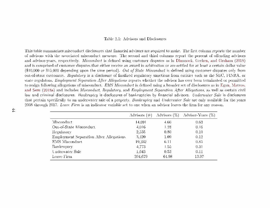
Table 2.1: Advisors and Disclosures
This table summarizes misconduct disclosures that �nancial advisors are required to make. The �rst column reports the numberof advisors with the associated misconduct measure. The second and third columns report the percent of o�ending advisorsand advisor-years, respectively. Misconduct is de�ned using customer disputes as in Dimmock, Gerken, and Graham (2018)and is comprised of customer disputes that either receive an award in arbitration or are settled for at least a certain dollar value($10,000 or $15,000 depending upon the time period). Out-of-State Misconduct is de�ned using customer disputes only fromout-of-state customers. Regulatory is a disclosure of �nalized regulatory sanctions from entities such as the SEC, FINRA, orstate regulators. Employment Separation After Allegations reports whether the advisor has ever been terminated or permittedto resign following allegations of misconduct. EMS Misconduct is de�ned using a broader set of disclosures as in Egan, Matvos,and Seru (2018a) and includes Misconduct, Regulatory, and Employment Separation After Allegations, as well as certain civillaw and criminal disclosures. Bankruptcy is disclosures of bankruptcies by �nancial advisors. Underwater Sale is disclosuresthat pertain speci�cally to an underwater sale of a property. Bankruptcy and Underwater Sale are only available for the years2008 through 2017. Leave Firm is an indicator variable set to one when an advisor leaves the �rm for any reason.
Advisors (#) Advisors (%) Advisor-Years (%)
Misconduct 14,691 4.66 0.63Out-of-State Misconduct 4,016 1.28 0.16Regulatory 2,535 0.80 0.10Employment Separation After Allegations 3,420 1.09 0.12EMS Misconduct 19,232 6.11 0.85Bankruptcy 4,773 1.55 0.31Underwater Sale 1,643 0.53 0.11Leave Firm 204,679 64.98 13.97
44
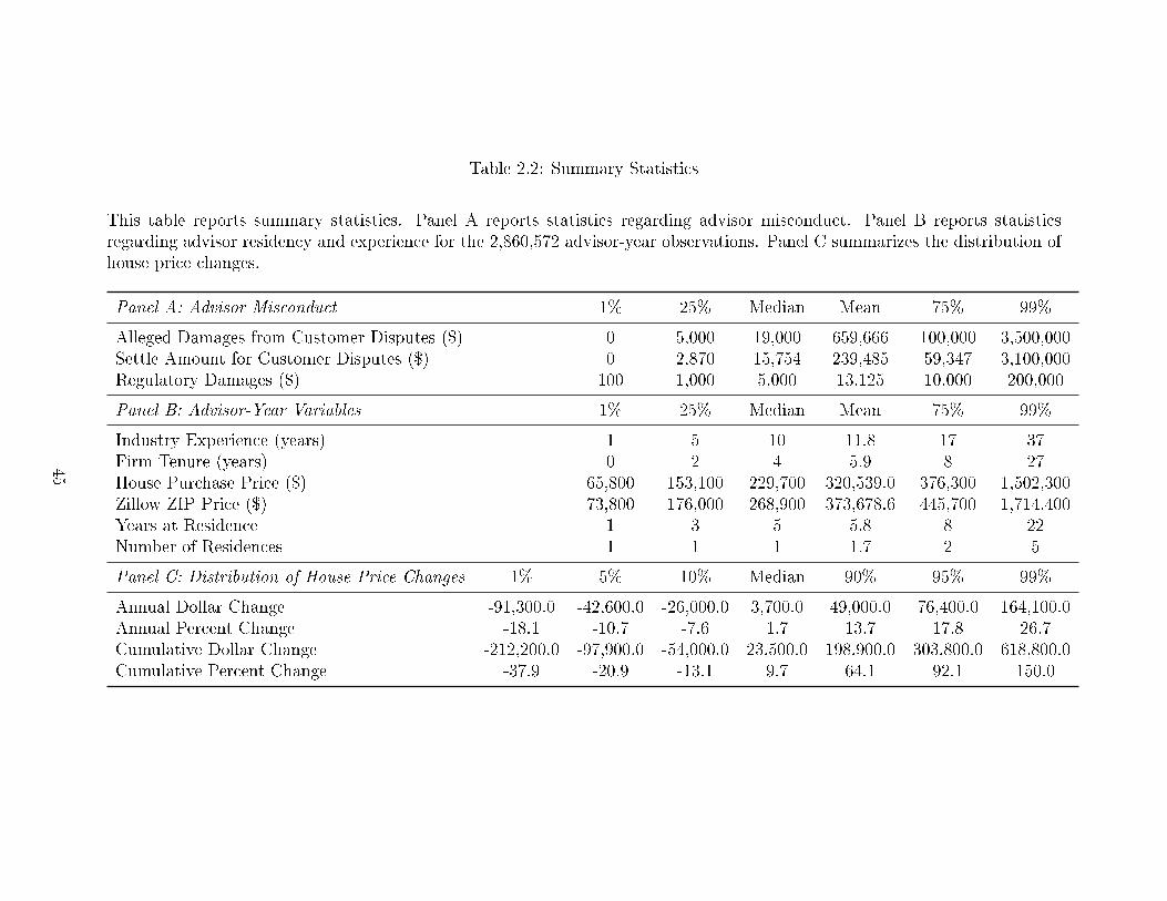
Table 2.2: Summary Statistics
This table reports summary statistics. Panel A reports statistics regarding advisor misconduct. Panel B reports statisticsregarding advisor residency and experience for the 2,860,572 advisor-year observations. Panel C summarizes the distribution ofhouse price changes.
Panel A: Advisor Misconduct 1% 25% Median Mean 75% 99%
Alleged Damages from Customer Disputes ($) 0 5,000 19,000 659,666 100,000 3,500,000Settle Amount for Customer Disputes ($) 0 2,870 15,754 239,485 59,347 3,100,000Regulatory Damages ($) 100 1,000 5,000 13,125 10,000 200,000
Panel B: Advisor-Year Variables 1% 25% Median Mean 75% 99%
Industry Experience (years) 1 5 10 11.8 17 37Firm Tenure (years) 0 2 4 5.9 8 27House Purchase Price ($) 65,800 153,100 229,700 320,539.0 376,300 1,502,300Zillow ZIP Price ($) 73,800 176,000 268,900 373,678.6 445,700 1,714,400Years at Residence 1 3 5 5.8 8 22Number of Residences 1 1 1 1.7 2 5
Panel C: Distribution of House Price Changes 1% 5% 10% Median 90% 95% 99%
Annual Dollar Change -91,300.0 -42,600.0 -26,000.0 3,700.0 49,000.0 76,400.0 164,100.0Annual Percent Change -18.1 -10.7 -7.6 1.7 13.7 17.8 26.7Cumulative Dollar Change -212,200.0 -97,900.0 -54,000.0 23,500.0 198,900.0 303,800.0 618,800.0Cumulative Percent Change -37.9 -20.9 -13.1 9.7 64.1 92.1 150.0
45
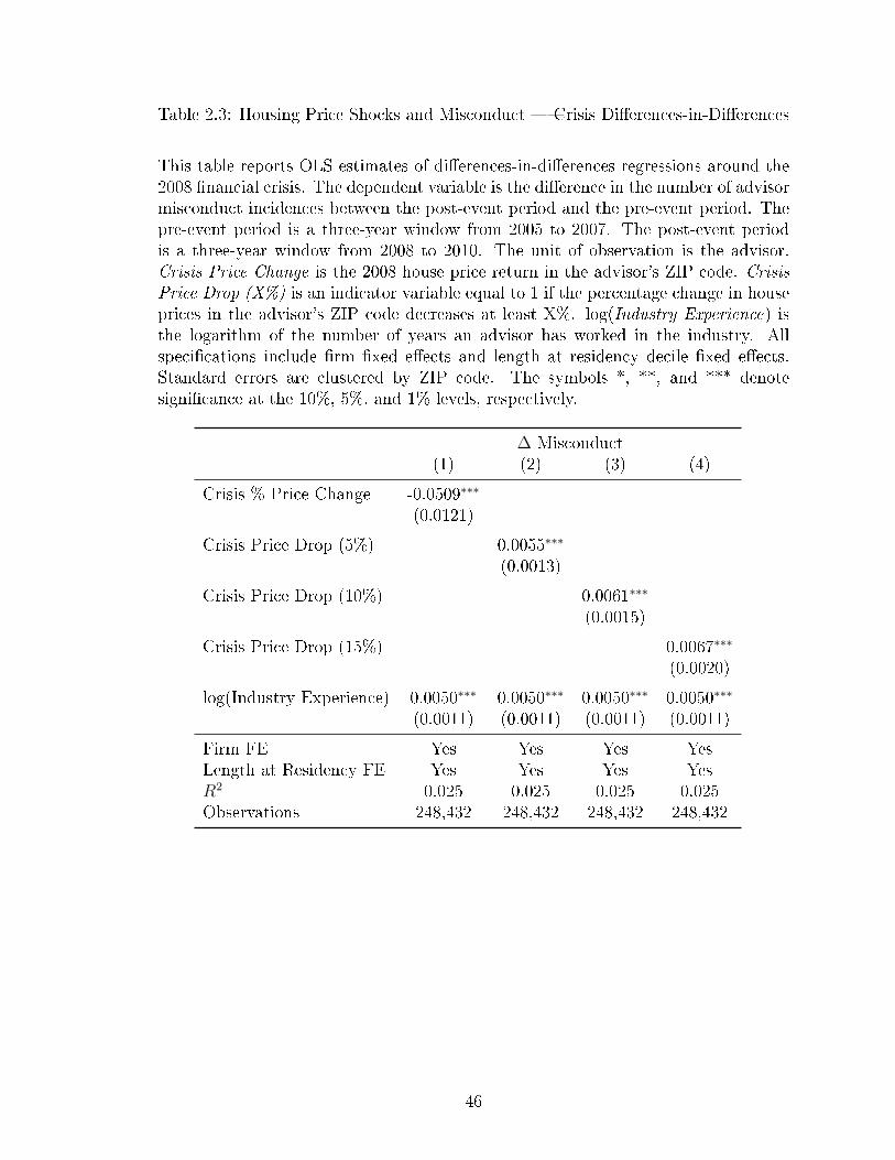
Table 2.3: Housing Price Shocks and Misconduct � Crisis Di�erences-in-Di�erences
This table reports OLS estimates of di�erences-in-di�erences regressions around the2008 �nancial crisis. The dependent variable is the di�erence in the number of advisormisconduct incidences between the post-event period and the pre-event period. Thepre-event period is a three-year window from 2005 to 2007. The post-event periodis a three-year window from 2008 to 2010. The unit of observation is the advisor.Crisis Price Change is the 2008 house price return in the advisor's ZIP code. CrisisPrice Drop (X%) is an indicator variable equal to 1 if the percentage change in houseprices in the advisor's ZIP code decreases at least X%. log(Industry Experience) isthe logarithm of the number of years an advisor has worked in the industry. Allspeci�cations include �rm �xed e�ects and length at residency decile �xed e�ects.Standard errors are clustered by ZIP code. The symbols *, **, and *** denotesigni�cance at the 10%, 5%, and 1% levels, respectively.
∆ Misconduct(1) (2) (3) (4)
Crisis % Price Change -0.0509∗∗∗
(0.0121)
Crisis Price Drop (5%) 0.0055∗∗∗
(0.0013)
Crisis Price Drop (10%) 0.0061∗∗∗
(0.0015)
Crisis Price Drop (15%) 0.0067∗∗∗
(0.0020)
log(Industry Experience) 0.0050∗∗∗ 0.0050∗∗∗ 0.0050∗∗∗ 0.0050∗∗∗
(0.0011) (0.0011) (0.0011) (0.0011)
Firm FE Yes Yes Yes YesLength at Residency FE Yes Yes Yes YesR2 0.025 0.025 0.025 0.025Observations 248,432 248,432 248,432 248,432
46

Table 2.4: Cumulative House Price Return and Misconduct
This table reports estimates from regressions of misconduct on an advisor's cumula-tive house price return since purchase. The unit of observation is the advisor-year.The dependent variable is an indicator variable for advisor misconduct (multipliedby 100). Cumulative Return is the aggregated cumulative price change divided bythe purchase price. In column (3), the speci�cation also includes an interaction term,(Cumulative Return − (−20%)) × IExtreme, where IExtreme indicates a cumulativereturn worse than -20%. log(Industry Experience) is the logarithm of the number ofyears an advisor has worked in the industry. Speci�cation (1) includes advisor controlvariables and �rm×year, ZIP code, and length at residency decile �xed e�ects. Thelatter speci�cations replace the advisor controls with advisor �xed e�ects. Standarderrors, clustered by advisor and ZIP code, are reported in parentheses. The symbols*, **, and *** denote signi�cance at the 10%, 5%, and 1% levels, respectively.
Misconduct(1) (2) (3)
Cumulative Return -0.0847∗∗∗ -0.2082∗∗∗ -0.1951∗∗∗
(0.0205) (0.0303) (0.0310)
Cumulative Return×IExtreme -0.4664∗
(0.2777)
log(Industry Experience) 0.2382∗∗∗ 0.4914∗∗∗ 0.4916∗∗∗
(0.0079) (0.0219) (0.0219)
Advisor Controls Yes No NoAdvisor FE No Yes YesLength at Residency FE Yes Yes YesFirm×Year FE Yes Yes YesZIP FE Yes Yes YesR2 0.032 0.146 0.146Observations 2,882,302 2,860,572 2,860,572
47
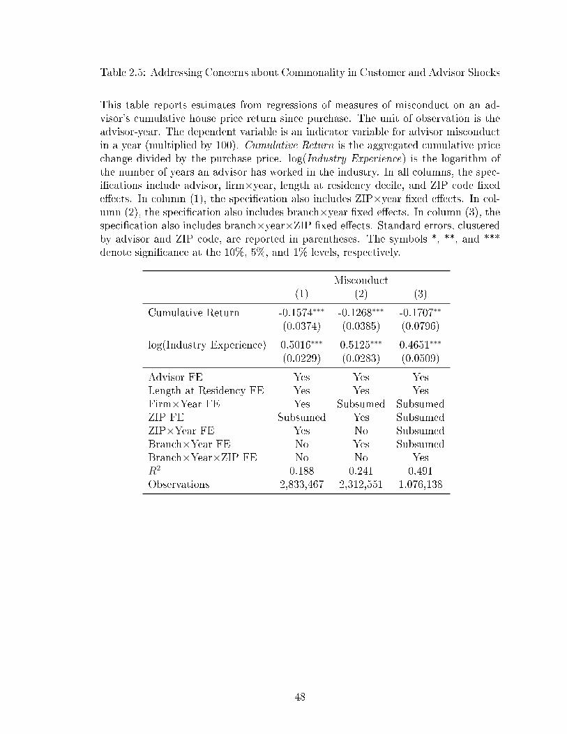
Table 2.5: Addressing Concerns about Commonality in Customer and Advisor Shocks
This table reports estimates from regressions of measures of misconduct on an ad-visor's cumulative house price return since purchase. The unit of observation is theadvisor-year. The dependent variable is an indicator variable for advisor misconductin a year (multiplied by 100). Cumulative Return is the aggregated cumulative pricechange divided by the purchase price. log(Industry Experience) is the logarithm ofthe number of years an advisor has worked in the industry. In all columns, the spec-i�cations include advisor, �rm×year, length at residency decile, and ZIP code �xede�ects. In column (1), the speci�cation also includes ZIP×year �xed e�ects. In col-umn (2), the speci�cation also includes branch×year �xed e�ects. In column (3), thespeci�cation also includes branch×year×ZIP �xed e�ects. Standard errors, clusteredby advisor and ZIP code, are reported in parentheses. The symbols *, **, and ***denote signi�cance at the 10%, 5%, and 1% levels, respectively.
Misconduct(1) (2) (3)
Cumulative Return -0.1574∗∗∗ -0.1268∗∗∗ -0.1707∗∗
(0.0374) (0.0385) (0.0796)
log(Industry Experience) 0.5016∗∗∗ 0.5125∗∗∗ 0.4651∗∗∗
(0.0229) (0.0283) (0.0509)
Advisor FE Yes Yes YesLength at Residency FE Yes Yes YesFirm×Year FE Yes Subsumed SubsumedZIP FE Subsumed Yes SubsumedZIP×Year FE Yes No SubsumedBranch×Year FE No Yes SubsumedBranch×Year×ZIP FE No No YesR2 0.188 0.241 0.491Observations 2,833,467 2,312,551 1,076,138
48

Table 2.6: Out-of-State Customers, Non-Customer Misconduct, and Advisor Shocks
This table reports estimates from regressions of measures of misconduct on an ad-visor's cumulative house price return since purchase. The unit of observation is theadvisor-year. In column (1), the dependent variable equals one if advisor misconductis reported by clients who live in a di�erent state than the advisor. In column (2),the dependent variable equals one if advisor misconduct is reported by clients wholive in a state that does not border the advisor's state. In column (3), the depen-dent variable equals one if a regulator or �rm reported incidences of misconduct. Incolumn (3), we exclude sample observations if a client also reports an incident ofmisconduct in the same year. In each column, we multiply the dependent variableby 100. Cumulative Return is the aggregated cumulative price change divided by thepurchase price. log(Industry Experience) is the logarithm of the number of years anadvisor has worked in the industry. In all columns, the speci�cations include advisor,�rm×year, length at residency decile, and ZIP code �xed e�ects. In column (3), thespeci�cation also includes state×year �xed e�ects. Standard errors, clustered by ad-visor and ZIP code, are reported in parentheses. The symbols *, **, and *** denotesigni�cance at the 10%, 5%, and 1% levels, respectively.
Out-of-State Distant Regulator orCustomer Customer Firm Actions
(1) (2) (3)
Cumulative Return -0.0463∗∗∗ -0.0351∗∗∗ -0.0441∗∗
(0.0149) (0.0126) (0.0181)
log(Industry Experience) 0.1064∗∗∗ 0.0736∗∗∗ 0.0643∗∗∗
(0.0100) (0.0084) (0.0134)
Advisor FE Yes Yes YesLength at Residency FE Yes Yes YesFirm×Year FE Yes Yes YesZIP FE Yes Yes YesState×Year FE No No YesR2 0.140 0.140 0.179Observations 2,860,572 2,860,604 2,842,344
49

Table 2.7: Cross-Sectional Variation in Termination Risk
This table reports estimates from regressions of misconduct on an advisor's cumula-tive house price return since purchase, interacted with indicator variables. The unitof observation is the advisor-year. The dependent variable is an indicator variable foradvisor misconduct (multiplied by 100). High Firm-Year is an indicator variable setto one if the �rm-year has an above average misconduct rate (excluding the advisor'sown misconduct). High Branch-Year is an indicator variable set to one if the branch-year has an above average misconduct rate (excluding the advisor's own misconduct).Branch is de�ned as a �rm-county. Female is an indicator variable for gender. PriorMisconduct is set to one if the advisor has ever had an incidence of misconduct inthe past. All speci�cations include advisor, �rm×year, length at residency decile,and ZIP code �xed e�ects. Standard errors, clustered by advisor and ZIP code, arereported in parentheses. The symbols *, **, and *** denote signi�cance at the 10%,5%, and 1% levels, respectively.
(1) (2) (3) (4)
Cumulative Return -0.1641∗∗∗ -0.1347∗∗∗ -0.2839∗∗∗ -0.0669∗∗∗
(0.0306) (0.0310) (0.0355) (0.0187)
High Firm-Year 5.1985∗∗∗
(0.3923)
C. Return×High Firm-Year -0.0849∗
(0.0467)
High Branch-Year 0.0671∗∗∗
(0.0239)
C. Return×High Branch-Year -0.1559∗∗∗
(0.0447)
C. Return×Female 0.3020∗∗∗
(0.0423)
Prior Misconduct 2.2214∗∗∗
(0.0647)
C. Return×Prior Misconduct -0.3556∗∗∗
(0.1265)
log(Industry Experience) 0.4892∗∗∗ 0.4900∗∗∗ 0.4922∗∗∗ 0.2696∗∗∗
(0.0219) (0.0219) (0.0220) (0.0066)
Advisor FE Yes Yes Yes NoLength at Residency FE Yes Yes Yes YesFirm×Year FE Yes Yes Yes YesZIP FE Yes Yes Yes YesR2 0.146 0.146 0.146 0.031Observations 2,860,572 2,860,572 2,843,273 2,882,302
50
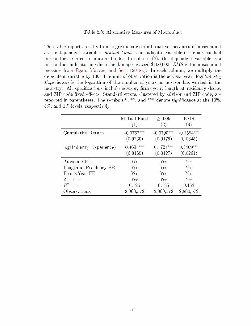
Table 2.8: Alternative Measures of Misconduct
This table reports results from regressions with alternative measures of misconductas the dependent variables. Mutual Fund is an indicator variable if the advisor hadmisconduct related to mutual funds. In column (2), the dependent variable is amisconduct indicator in which the damages exceed $100,000. EMS is the misconductmeasure from Egan, Matvos, and Seru (2018a). In each column, we multiply thedependent variable by 100. The unit of observation is the advisor-year. log(IndustryExperience) is the logarithm of the number of years an advisor has worked in theindustry. All speci�cations include advisor, �rm×year, length at residency decile,and ZIP code �xed e�ects. Standard errors, clustered by advisor and ZIP code, arereported in parentheses. The symbols *, **, and *** denote signi�cance at the 10%,5%, and 1% levels, respectively.
Mutual Fund ≥100k EMS(1) (2) (3)
Cumulative Return -0.0767∗∗∗ -0.0795∗∗∗ -0.2584∗∗∗
(0.0230) (0.0179) (0.0345)
log(Industry Experience) 0.4694∗∗∗ 0.1724∗∗∗ 0.5469∗∗∗
(0.0169) (0.0127) (0.0261)
Advisor FE Yes Yes YesLength at Residency FE Yes Yes YesFirm×Year FE Yes Yes YesZIP FE Yes Yes YesR2 0.126 0.135 0.163Observations 2,860,572 2,860,572 2,860,572
51

Table 2.9: Predicting Real Outcomes
This table tests whether our cumulative return measure reliably predicts negative �nancial outcomes for advisors. The unitof observation is the advisor-year. In column (1), the dependent variable, Bankruptcy, is an indicator equal to one if theadvisor reports a bankruptcy or other compromise with creditors. In column (2), the dependent variable, Underwater Sale,is an indicator equal to one if the advisor reports an underwater home sales (for which the advisor does not make the lenderwhole). Termination is an indicator equal to one if the advisor was terminated or permitted to resign following allegations ofmisconduct. Leave Firm is an indicator equal to one if the advisor left the �rm for any reason. In all columns, the dependentvariable is multiplied by 100. For data availability reasons, columns (1) and (2) are only estimated starting in 2008. log(IndustryExperience) is the logarithm of the number of years an advisor has worked in the industry. All speci�cations include advisor,�rm×year, length at residency decile, and ZIP code �xed e�ects. Standard errors, clustered by advisor and ZIP code, arereported in parentheses. The symbols *, **, and *** denote signi�cance at the 10%, 5%, and 1% levels, respectively.
Bankruptcy Underwater Sale Termination Leave Firm(1) (2) (3) (4)
Cumulative Return -0.3120∗∗∗ -0.3962∗∗∗ -0.0247∗∗ -1.7784∗∗∗
(0.0703) (0.0536) (0.0114) (0.1205)
log(Industry Experience) -0.1137∗∗ 0.0939∗∗∗ 0.0603∗∗∗ -1.0217∗∗∗
(0.0515) (0.0300) (0.0100) (0.1099)
Advisor FE Yes Yes Yes YesLength at Residency FE Yes Yes Yes YesFirm×Year FE Yes Yes Yes YesZIP FE Yes Yes Yes YesR2 0.263 0.274 0.140 0.380Observations 1,272,337 1,272,337 3,486,167 3,486,167
52

Figure 2.1: Real Estate Price Shocks by Year
This �gure plots the fraction of �nancial advisors whose residence experiences a year-over-year decline in price of at least 10% during the sample period, as measured bythe Zillow ZIP code level house price index. We plot this measure separately for theentire U.S. (black) and select states.
1998 2000 2002 2004 2006 2008 2010 2012 2014
0.2
0.4
0.6
0.8
1.0
Fractionof
shocked
advisors
Entire US Nevada Texas Illinois
53
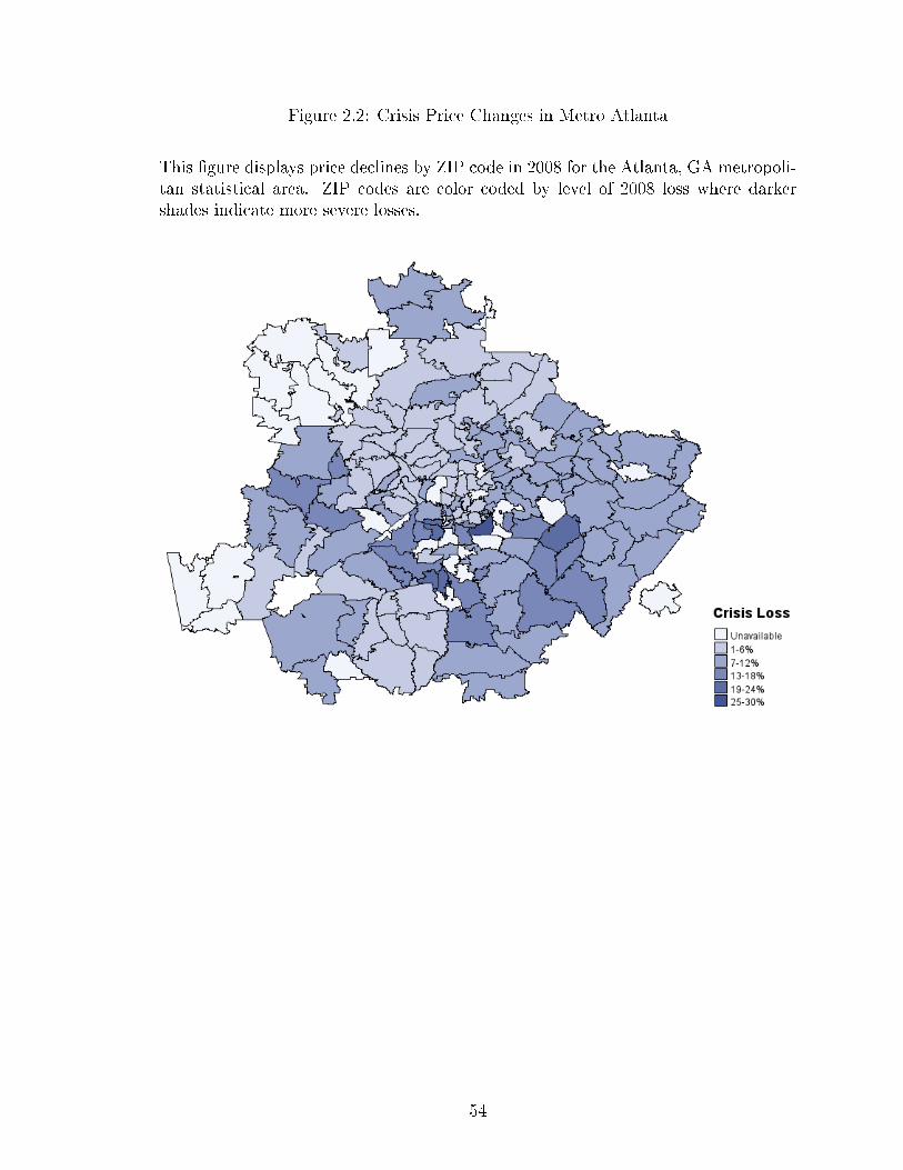
Figure 2.2: Crisis Price Changes in Metro Atlanta
This �gure displays price declines by ZIP code in 2008 for the Atlanta, GA metropoli-tan statistical area. ZIP codes are color coded by level of 2008 loss where darkershades indicate more severe losses.
54
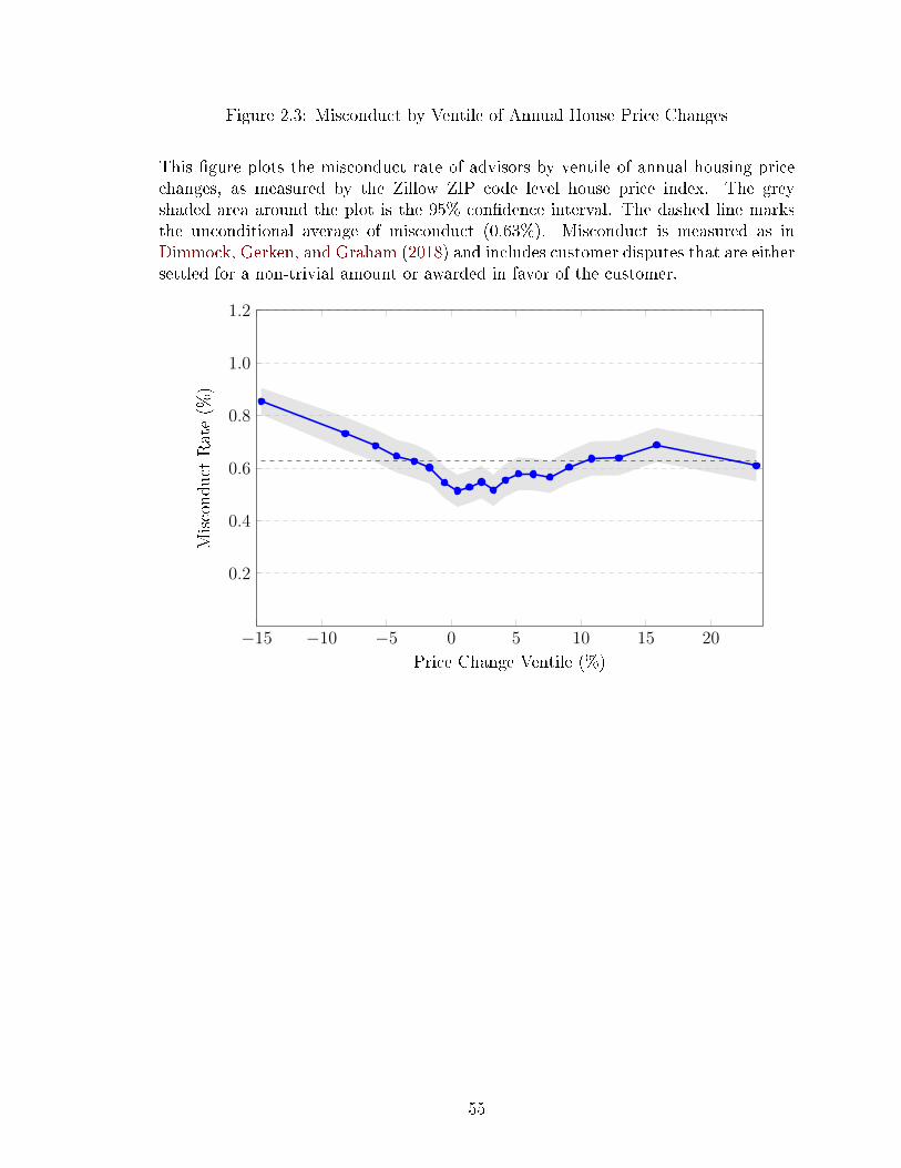
Figure 2.3: Misconduct by Ventile of Annual House Price Changes
This �gure plots the misconduct rate of advisors by ventile of annual housing pricechanges, as measured by the Zillow ZIP code level house price index. The greyshaded area around the plot is the 95% con�dence interval. The dashed line marksthe unconditional average of misconduct (0.63%). Misconduct is measured as inDimmock, Gerken, and Graham (2018) and includes customer disputes that are eithersettled for a non-trivial amount or awarded in favor of the customer.
−15 −10 −5 0 5 10 15 20
0.2
0.4
0.6
0.8
1.0
1.2
Price Change Ventile (%)
Misconduct
Rate(%
)
55

Figure 2.4: Misconduct Timing around Real Estate Shocks
This �gure plots the average misconduct rate in event time, where the event is a 10%or worse decline in an advisor's house price, as measured by the Zillow ZIP code levelhouse price index. The �gure plots three years before and three years after the event.The grey shaded area around the plot is the 95% con�dence interval. The dashed linemarks the unconditional average of misconduct (0.63%). Misconduct is measured asin Dimmock, Gerken, and Graham (2018) and includes customer disputes that areeither settled for a non-trivial amount or awarded in favor of the customer.
−3 −2 −1 0 1 2 3
0.2
0.4
0.6
0.8
1.0
1.2
Event Time (years)
Misconduct
Rate(%
)
56
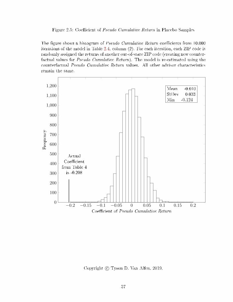
Figure 2.5: Coe�cient of Pseudo Cumulative Return in Placebo Samples
The �gure shows a histogram of Pseudo Cumulative Return coe�cients from 10,000iterations of the model in Table 2.4, column (2). For each iteration, each ZIP code israndomly assigned the returns of another out-of-state ZIP code (creating new counter-factual values for Pseudo Cumulative Return). The model is re-estimated using thecounterfactual Pseudo Cumulative Return values. All other advisor characteristicsremain the same.
−0.2 −0.15 −0.1 −0.05 0 0.05 0.1 0.15 0.20
100
200
300
400
500
600
700
800
900
1,000
1,100
1,200
Coe�cient of Pseudo Cumulative Return
Frequency
ActualCoe�cientfrom Table 4is -0.208
Mean = -0.010StDev = 0.033Min = -0.124
Copyright c© Tyson D. Van Alfen, 2019.
57

Appendix A: Example Observation for Chapter 1
58

Chapter 1 Internet Appendix
59

Table IA1.1: Details on Estimates for All Control Variables
This table presents all results from estimating Equation (1.1) and its variants. SeeTable 1.3. The dependent variable in columns (1) and (2) is measured as the averagenumber of stars (out of 5) assigned to the product in the subsequent year. Columns(3) and (4) use reputation as measured by the Helpful reviews. Any Vesting Eventis an indicator variable set to 1 in any year in which the �rm's CEO has either astock vesting event or an option vesting event. Any Stock Vesting and Any OptionVesting decompose Any Vesting Event accordingly. See the data section for detailedvariable de�nitions. Control variables are included in the speci�cations and de�nedin the text. Indicators for �xed e�ects are reported at the bottom of the table, andstandard errors, clustered at the product level, are reported in parentheses. Asterisksrepresent the conventional levels of statistical signi�cance.
Reputationt+1 Helpful Reputationt+1
(1) (2) (3) (4)
Any Vesting Event -0.067∗∗∗ -0.070∗∗∗
(0.018) (0.017)
Stock Vesting -0.101∗∗∗ -0.098∗∗∗
(0.020) (0.020)
Option Vesting 0.022 -0.008(0.029) (0.031)
Book-to-Market 0.061 0.062 -0.011 -0.011(0.041) (0.041) (0.044) (0.044)
Operating Margin 0.061 0.067 0.115 0.119(0.106) (0.106) (0.115) (0.115)
Leverage -0.150 -0.137 -0.163 -0.154(0.117) (0.117) (0.123) (0.123)
LN(Market Cap) -0.069∗∗∗ -0.068∗∗∗ -0.052∗∗ -0.052∗∗
(0.019) (0.019) (0.023) (0.023)
12-month Return 0.010 0.008 0.005 0.004(0.014) (0.014) (0.014) (0.014)
R&D 0.798∗∗ 0.854∗∗∗ 1.167∗∗∗ 1.210∗∗∗
(0.311) (0.313) (0.380) (0.384)
Controls Yes Yes Yes YesFirm FE Yes Yes Yes YesYear FE Yes Yes Yes YesR2 0.063 0.063 0.066 0.067Observations 52,924 52,924 50,168 50,168
60
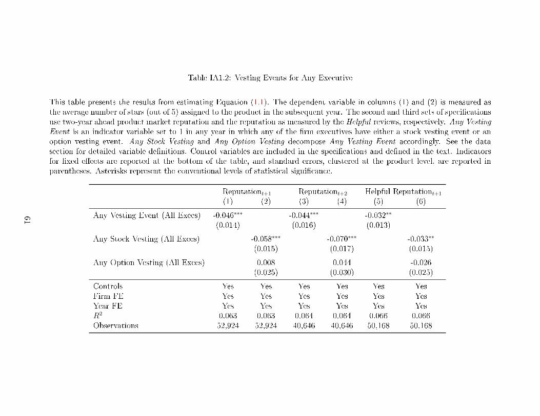
Table IA1.2: Vesting Events for Any Executive
This table presents the results from estimating Equation (1.1). The dependent variable in columns (1) and (2) is measured asthe average number of stars (out of 5) assigned to the product in the subsequent year. The second and third sets of speci�cationsuse two-year ahead product market reputation and the reputation as measured by the Helpful reviews, respectively. Any VestingEvent is an indicator variable set to 1 in any year in which any of the �rm executives have either a stock vesting event or anoption vesting event. Any Stock Vesting and Any Option Vesting decompose Any Vesting Event accordingly. See the datasection for detailed variable de�nitions. Control variables are included in the speci�cations and de�ned in the text. Indicatorsfor �xed e�ects are reported at the bottom of the table, and standard errors, clustered at the product level, are reported inparentheses. Asterisks represent the conventional levels of statistical signi�cance.
Reputationt+1 Reputationt+2 Helpful Reputationt+1
(1) (2) (3) (4) (5) (6)
Any Vesting Event (All Execs) -0.046∗∗∗ -0.044∗∗∗ -0.032∗∗
(0.014) (0.016) (0.013)
Any Stock Vesting (All Execs) -0.058∗∗∗ -0.070∗∗∗ -0.033∗∗
(0.015) (0.017) (0.015)
Any Option Vesting (All Execs) 0.008 0.044 -0.026(0.025) (0.030) (0.025)
Controls Yes Yes Yes Yes Yes YesFirm FE Yes Yes Yes Yes Yes YesYear FE Yes Yes Yes Yes Yes YesR2 0.063 0.063 0.064 0.064 0.066 0.066Observations 52,924 52,924 40,646 40,646 50,168 50,168
61

Chapter 2 Internet Appendix
Table IA2.1: Home Ownership
This table reports estimates from regressions of misconduct on an advisor's cumu-lative house price change since purchase for subsamples of our dataset. The unit ofobservation is the advisor-year. The dependent variable is an indicator variable foradvisor misconduct in the current year (multiplied by 100). Cumulative Return is theaggregated cumulative price change divided by the purchase price. In column (1),we exclude ZIP codes with low levels of home ownership (<50%) as reported in theAmerican Community Survey. In column (2), we exclude multi-dwelling unit (MDU)addresses (e.g., apartment buildings). log(Industry Experience) is the logarithm ofthe number of years an advisor has worked in the industry. All speci�cations includeadvisor, �rm×year, length at residency decile, and ZIP code �xed e�ects. Standarderrors, clustered by advisor and ZIP code, are reported in parentheses. The symbols*, **, and *** denote signi�cance at the 10%, 5%, and 1% levels, respectively.
Dependent Variable: Misconduct(1) (2)
Cumulative Return -0.2054*** -0.2076***(0.0364) (0.0332)
log(Industry Experience) 0.5174*** 0.5007***(0.0249) (0.0240)
Advisor FE Yes YesLength at Residency FE Yes YesFirm×Year FE Yes YesZIP FE Yes YesExclude Low Ownership ZIPs Yes NoExclude MDUs No YesR-squared 0.151 0.151Observations 2,342,187 2,522,052
62

Table IA2.2: Federal Housing Price Index
This table reports estimates from regressions of misconduct on an advisor's cumula-tive house price return since purchase. The unit of observation is the advisor-year.Column (1) reports OLS estimates of di�erences-in-di�erences regressions around the2008 �nancial crisis. The dependent variable is the di�erence in the number of advisormisconduct incidences between the post-event period and the pre-event period. Thepre-event period is a three-year window from 2005 to 2007. The post-event periodis a three-year window from 2008 to 2010. The dependent variable for columns (2)and (3) is an indicator variable for advisor misconduct (multiplied by 100). CrisisPrice Change is the 2008 house price return in the advisor's ZIP code. CumulativeReturn is the aggregated cumulative price change divided by the purchase price. Bothmeasures of house price returns use the House Price Index produced by the FederalHousing Finance Agency instead of Zillow estimates. log(Industry Experience) is thelogarithm of the number of years an advisor has worked in the industry. The presenceof control variables and �xed e�ects is indicated at the bottom of the table. Standarderrors, clustered by advisor and ZIP code, are reported in parentheses. The symbols*, **, and *** denote signi�cance at the 10%, 5%, and 1% levels, respectively.
Dependent Variable: ∆Misconduct Misconduct Misconduct(1) (2) (3)
Crisis Price Change -0.0491***(0.0106)
Cumulative Return -0.0427*** -0.0706***(0.0118) (0.0210)
log(Industry Experience) 0.0046*** 0.2473*** 0.4952***(0.0011) (0.0067) (0.0181)
Advisor Controls No Yes NoAdvisor FE Yes No YesFirm FE Yes Subsumed SubsumedFirm×Year FE No Yes YesLength at Residency FE Yes Yes YesZIP FE No Yes YesR2 0.025 0.029 0.131Observations 252,183 3,737,534 3,716,283
63
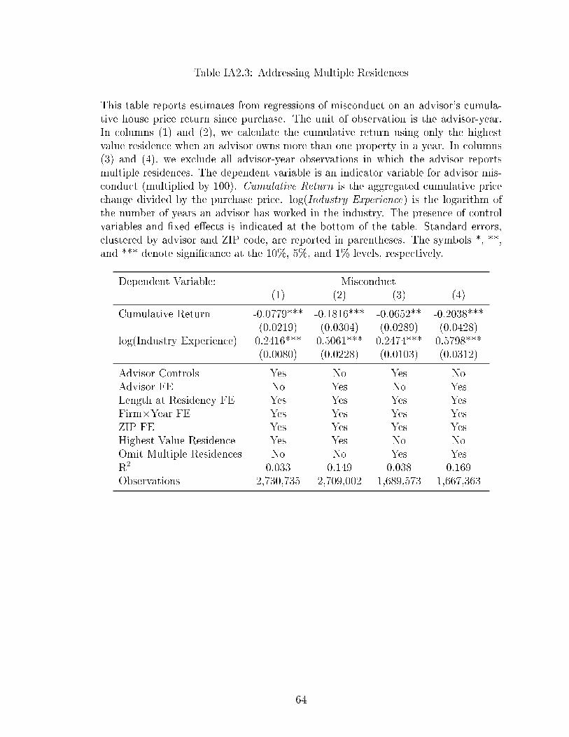
Table IA2.3: Addressing Multiple Residences
This table reports estimates from regressions of misconduct on an advisor's cumula-tive house price return since purchase. The unit of observation is the advisor-year.In columns (1) and (2), we calculate the cumulative return using only the highestvalue residence when an advisor owns more than one property in a year. In columns(3) and (4), we exclude all advisor-year observations in which the advisor reportsmultiple residences. The dependent variable is an indicator variable for advisor mis-conduct (multiplied by 100). Cumulative Return is the aggregated cumulative pricechange divided by the purchase price. log(Industry Experience) is the logarithm ofthe number of years an advisor has worked in the industry. The presence of controlvariables and �xed e�ects is indicated at the bottom of the table. Standard errors,clustered by advisor and ZIP code, are reported in parentheses. The symbols *, **,and *** denote signi�cance at the 10%, 5%, and 1% levels, respectively.
Dependent Variable: Misconduct(1) (2) (3) (4)
Cumulative Return -0.0779*** -0.1816*** -0.0652** -0.2038***(0.0219) (0.0304) (0.0289) (0.0428)
log(Industry Experience) 0.2416*** 0.5061*** 0.2474*** 0.5798***(0.0080) (0.0228) (0.0103) (0.0312)
Advisor Controls Yes No Yes NoAdvisor FE No Yes No YesLength at Residency FE Yes Yes Yes YesFirm×Year FE Yes Yes Yes YesZIP FE Yes Yes Yes YesHighest Value Residence Yes Yes No NoOmit Multiple Residences No No Yes YesR2 0.033 0.149 0.038 0.169Observations 2,730,735 2,709,002 1,689,573 1,667,363
64

Table IA2.4: Alternate Di�erences in Di�erences Speci�cations
This table reports OLS estimates of di�erences-in-di�erences regressions around the�nancial crisis. The dependent variable is the di�erence in the number of advisormisconduct incidences between the post-event period and the pre-event period. Incolumn (1), we follow Pool, Sto�man, Yonker, and Zhang (2018), who de�ne thepre-period as 2005�2006 and the post-period as 2009�2010. In column (2), we followBernstein, McQuade, and Townsend (2018), who de�ne the pre-period as 2005�2007and the post-period as 2008�2012. Column (3) is similar to our main speci�cationin Table 3, except that we introduce a gap year: the pre-event period is a three-yearwindow from 2005 to 2007, and the post-event period is a three-year window from 2009to 2011. The unit of observation is the advisor. Crisis Price Change is the 2008 houseprice return in the advisor's ZIP code. log(Industry Experience) is the logarithm ofthe number of years an advisor has worked in the industry. All speci�cations include�rm �xed e�ects and length at residency decile �xed e�ects. Standard errors areclustered by ZIP code. The symbols *, **, and *** denote signi�cance at the 10%,5%, and 1% levels, respectively.
Dependent Variable: ∆MisconductPSYZ BMT Gap Year(1) (2) (3)
Crisis Price Change -0.0289*** -0.0678*** -0.0366***(0.0103) (0.0147) (0.0120)
log(Industry Experience) 0.0022** 0.0119*** 0.0035***(0.0009) (0.0014) (0.0011)
Firm FE Yes Yes YesLength at Residency FE Yes Yes YesR2 0.022 0.030 0.027Observations 248,432 247,514 248,432
65
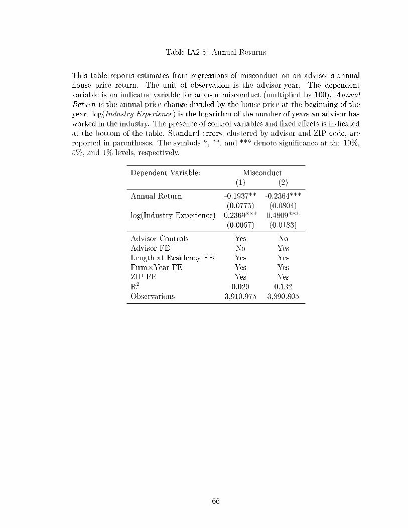
Table IA2.5: Annual Returns
This table reports estimates from regressions of misconduct on an advisor's annualhouse price return. The unit of observation is the advisor-year. The dependentvariable is an indicator variable for advisor misconduct (multiplied by 100). AnnualReturn is the annual price change divided by the house price at the beginning of theyear. log(Industry Experience) is the logarithm of the number of years an advisor hasworked in the industry. The presence of control variables and �xed e�ects is indicatedat the bottom of the table. Standard errors, clustered by advisor and ZIP code, arereported in parentheses. The symbols *, **, and *** denote signi�cance at the 10%,5%, and 1% levels, respectively.
Dependent Variable: Misconduct(1) (2)
Annual Return -0.1937** -0.2364***(0.0775) (0.0804)
log(Industry Experience) 0.2369*** 0.4809***(0.0067) (0.0183)
Advisor Controls Yes NoAdvisor FE No YesLength at Residency FE Yes YesFirm×Year FE Yes YesZIP FE Yes YesR2 0.029 0.132Observations 3,910,975 3,890,805
66

Table IA2.6: One-Year Ahead & Three-Year Misconduct
This table reports estimates from regressions of misconduct on an advisor's cumula-tive house price return since purchase. The unit of observation is the advisor-year.In columns (1) and (2), the dependent variable is an indicator variable for advisormisconduct (multiplied by 100) in the subsequent year. In columns (3) and (4), thedependent variable is an indicator variable for advisor misconduct (multiplied by 100)in the three year window from t=0 to t=2. Cumulative Return is the aggregated cu-mulative price change divided by the purchase price. log(Industry Experience) is thelogarithm of the number of years an advisor has worked in the industry. The presenceof control variables and �xed e�ects is indicated at the bottom of the table. Standarderrors, clustered by advisor and ZIP code, are reported in parentheses. The symbols*, **, and *** denote signi�cance at the 10%, 5%, and 1% levels, respectively.
Dependent Variable: Misconduct1 Misconduct0�2(1) (2) (3) (4)
Cumulative Return -0.0516** -0.1451*** -0.1454*** -0.3605***(0.0207) (0.0306) (0.0508) (0.0691)
log(Industry Experience) 0.2006*** 0.4569*** 0.5668*** 1.2585***(0.0082) (0.0224) (0.0209) (0.0519)
Advisor Controls Yes No Yes NoAdvisor FE No Yes No YesLength at Residency FE Yes Yes Yes YesFirm×Year FE Yes Yes Yes YesZIP FE Yes Yes Yes YesR2 0.031 0.149 0.054 0.326Observations 2,882,302 2,860,572 2,882,302 2,860,572
67

Table IA2.7: Estimates for All Control Variables
This table reports the full control variable estimates from the regression of misconducton an advisor's cumulative house price return since purchase from Column (1) ofTable 2.4. See Table 2.4 for details.
Dependent Variable: Misconduct
Cumulative Return -0.0847∗∗∗
(0.0205)
log(Industry Experience) 0.2382∗∗∗
(0.0079)
Female -0.3237∗∗∗
(0.0106)
Age -0.0014∗∗
(0.0007)
Series 6 0.0141(0.0157)
Series 7 0.0956∗∗∗
(0.0168)
Series 24 -0.0891∗∗∗
(0.0168)
Series 65 0.2749∗∗∗
(0.0163)
Series 66 0.1010∗∗∗
(0.0147)
Firm×Year, ZIP, Missing Demographic & Length at Residency FE Yes
R2 0.032Observations 2,882,302
68
References
Ajinkya, Bipin, Sanjeev Bhojraj, and Partha Sengupta, 2005, The association be-tween outside directors, institutional investors and the properties of managementearnings forecasts, Journal of Accounting Research 43, 343�376.
Bergstresser, Daniel, John Chalmers, and Peter Tufano, 2009, Assessing the costsand bene�ts of brokers in the mutual fund industry, Review of Financial Studies22, 4129�4156.
Bernstein, Shai, Timothy McQuade, and Richard R. Townsend, 2018, Do householdwealth shocks a�ect productivity? Evidence from innovative workers during thegreat recession, Working paper.
Bertrand, Marianne, Esther Du�o, and Sendhil Mullainathan, 2004, How much shouldwe trust di�erences-in-di�erences estimates?, Quarterly Journal of Economics 119,249�275.
Block, Michael K., and John M. Heineke, 1975, A labor theoretic analysis of thecriminal choice, American Economic Review 65, 314�325.
Block, Michael K., and Robert C. Lind, 1975, Crime and punishment reconsidered,Journal of Legal Studies 4, 241�247.
Bogin, Alexander N., William M. Doerner, and William D. Larson, 2018, Local houseprice dynamics: New indices and stylized facts, Real Estate Economics forthcom-ing.
Bushee, Brian J., 1998, The in�uence of institutional investors on myopic R&D in-vestment behavior, Accounting review 305�333.
Bushee, Brian J, 2001, Do institutional investors prefer near-term earnings over long-run value?, Contemporary Accounting Research 18, 207�246.
Campbell, John Y., and Joao F. Cocco, 2007, How do house prices a�ect consump-tion? Evidence from micro data, Journal of Monetary Economics 54, 591�621.
Campbell, John Y., Stefano Giglio, and Parag Pathak, 2011, Forced sales and houseprices, American Economic Review 101, 2108�2131.
Carroll, Christopher D., Misuzu Otsuka, and Jiri Slacalek, 2011, How large are hous-ing and �nancial wealth e�ects? A new approach, Journal of Money, Credit andBanking 43, 55�79.
Cavallo, Alberto, 2018, More amazon e�ects: Online competition and pricing behav-iors, Working Paper.
69
Cella, Cristina, 2009, Institutional investors and corporate investment, Working Pa-per.
Chal�n, Aaron, and Justin McCrary, 2017, Criminal deterrence: A review of theliterature, Journal of Economic Literature 55, 5�48.
Chalmers, John, and Jonathan Reuter, 2015, Is con�icted investment advice betterthan no advice?, Working Paper 18158, NBER.
Charoenwong, Ben, Alan Kwan, and Tarik Umar, 2018, Regulator jurisdiction andinvestment advisor misconduct, Working paper.
Chen, Pei-yu, Samita Dhanasobhon, and Michael D. Smith, 2008, All reviews are notcreated equal: The disaggregate impact of reviews and reviewers at Amazon.com,Working Paper.
Cheng, Ing-Haw, Sahil Raina, and Wei Xiong, 2014, Wall street and the housingbubble, American Economic Review 104, 2797�2829.
Cli�ord, Christopher P, 2008, Value creation or destruction? Hedge funds as share-holder activists, Journal of Corporate Finance 14, 323�336.
Cli�ord, Christopher P., and William C. Gerken, 2018, Investment in human capitaland labor mobility: Evidence from a shock to property rights, Working Paper.
Cressey, Donald R., 1971, Other Peoples' Money: A Study of the Social Psychologyof Embezzlement (Glencoe: Free Press).
DeFusco, Anthony A., 2018, Homeowner borrowing and housing collateral: Newevidence from expiring price controls, Journal of Finance 73, 523�573.
Derrien, François, Ambrus Kecskés, and David Thesmar, 2013, Investor horizons andcorporate policies, Journal of Financial and Quantitative Analysis 48, 1755�1780.
Dimmock, Stephen G., William C. Gerken, and Nathaniel P. Graham, 2018, Is fraudcontagious? Career network and fraud by �nancial advisors, Journal of Finance73, 1417�1450.
Edlund, Lena, Cecilia Machado, and Maria Sviatschi, 2019, Bright minds, big rent:Gentri�cation and the rising returns to skill, Working paper 21729, NBER.
Edmans, Alex, 2009, Blockholder trading, market e�ciency, and managerial myopia,The Journal of Finance 64, 2481�2513.
Edmans, Alex, Vivian W Fang, and Katharina A Lewellen, 2017, Equity vesting andinvestment, Review of Financial Studies 30, 2229�2271.
Egan, Mark, Gregor Matvos, and Amit Seru, 2018a, The market for �nancial advisermisconduct, Journal of Political Economy forthcoming.
70
Egan, Mark, Gregor Matvos, and Amit Seru, 2018b, When Harry �red Sally: Thedouble standard in punishing misconduct, Working Paper.
Fich, Eliezer M., and Anil Shivdasani, 2007, Financial fraud, director reputation, andshareholder wealth, Journal of Financial Economics 86, 306�336.
Foerster, Stephen, Juhani T. Linnainmaa, Brian T. Melzer, and Alessandro Previtero,2017, Retail �nancial advice: Does one size �t all?, Journal of Finance 72, 1441�1482.
Gan, Jie, 2010, Housing wealth and consumption growth: Evidence from a large panelof households, Review of Financial Studies 23, 2229�2267.
Gaspar, José-Miguel, Massimo Massa, and Pedro Matos, 2005, Shareholder invest-ment horizons and the market for corporate control, Journal of Financial Eco-nomics 76, 135�165.
Gennaioli, Nicola, Andrei Shleifer, and Robert Vishny, 2015, Money doctors, Journalof Finance 70, 91�114.
Gerardi, Kristopher, Kyle F. Herkenho�, Lee E. Ohanian, and Paul S. Willen, 2018,Can't pay or won't pay? Unemployment, negative equity, and strategic default,Review of Financial Studies 31, 1098�1131.
Gerken, William C., Laura T. Starks, and Michael C. Yates, 2018, The importance offamily: The role of mutual fund family reputation in investment decision, WorkingPaper.
Giannetti, Mariassunta, and Tracy Yue Wang, 2016, Corporate scandals and house-hold stock market participation, Journal of Finance 71, 2591�2636.
Giles, Jim, 2005, Internet encyclopaedias go head to head, Nature 438, 900�901.
Graham, John R., Campbell R. Harvey, and Shiva Rajgopal, 2005, The economicimplications of corporate �nancial reporting, Journal of Accounting and Economics40, 3�73.
Gurun, Umit G., Noah Sto�man, and Scott E. Yonker, 2018, Trust busting: Thee�ect of fraud on investor behavior, Review of Financial Studies 31, 1341�1376.
Hackethal, Andreas, Michael Haliassos, and Tullio Jappelli, 2012, Financial advisors:A case of babysitters?, Journal of Banking & Finance 36, 509�524.
Hackethal, Andreas, Roman Inderst, and Ste�en Meyer, 2011, Trading on advice,Working paper.
Hoechle, Daniel, Stefan Ruenzi, Nic Schaub, and Markus Schmid, 2018, Financialadvice and bank pro�ts, Review of Financial Studies 31, 4447�4492.
71

Huang, Jiekun, 2018, The customer knows best: The investment value of consumeropinions, Journal of Financial Economics 128, 164�182.
Hung, Angela A., Noreen Clancy, Je� Dominitz, Eric Talley, Claude Berribi, andFarrukh Suvankulov, 2008, Investor and industry perspectives on investment advi-sors and broker-dealers, Technical Report RAND Center for Corporate Ethics andGovernance .
Inderst, Roman, and Marco Ottaviani, 2009, Misselling through agents, AmericanEconomic Review 99, 883�908.
Inderst, Roman, and Marco Ottaviani, 2012, How (not) to pay for advice: A frame-work for consumer �nancial protection, Journal of Financial Economics 105, 393�411.
Jame, Russell, Rick Johnston, Stanimir Markov, and Michael Wolfe, 2016, The valueof crowdsourced earnings forecasts, Journal of Accounting Research 54, 1077�1110.
Jensen, Michael C., and William H. Meckling, 1976, Theory of the �rm: Managerialbehavior, agency costs and ownership structure, Journal of Financial Economics3, 305�360.
Karpo�, Jonathan M., D. Scott Lee, and Gerald S. Martin, 2008, The consequencesto managers for �nancial misrepresentation, Journal of Financial Economics 43,581�612.
Kau, James B., Donald C. Keenan, and Taewon Kim, 1994, Default probabilities formortgages, Journal of Urban Economics 35, 278�296.
Larkin, Yelena, 2013, Brand perception, cash �ow stability, and �nancial policy,Journal of Financial Economics 110, 232�253.
Lev, Baruch, Christine Petrovits, and Suresh Radhakrishnan, 2010, Is doing goodgood for you? How corporate charitable contributions enhance revenue growth,Strategic Management Journal 31, 182�200.
Matsa, David A, 2011, Running on empty? Financial leverage and product quality inthe supermarket industry, American Economic Journal: Microeconomics 3, 137�73.
Maturana, Gonzalo, and Jordan Nickerson, 2018, Real e�ects of worker's �nancialdistress: Evidence from teacher spillovers, Working paper.
McAuley, Julian, and Jure Leskovec, 2013, Hidden factors and hidden topics: Un-derstanding rating dimensions with review text, in Proceedings of the 7th ACMConference on Recommender Systems , 165�172, ACM.
Melnik, Mikhail I., and James Alm, 2002, Does a seller's ecommerce reputation mat-ter? Evidence from eBay auctions, Journal of Industrial Economics 50, 337�349.
72

Mian, Atif, Kamalesh Rao, and Amir Su�, 2013, Household balance sheets, consump-tion, and the economic slump, Quarterly Journal of Economics 128, 1687�1726.
Moore, David, 2018, Managerial self-interest and strategic repurchases: Evidencefrom equity vesting schedules, Working Paper.
Morrison, Alan D., and John Thanassoulis, 2017, Ethical standards and culturalassimilation in �nancial services, Working paper.
Mullainathan, Sendhil, Markus Noeth, and Antoinette Schoar, 2012, The market for�nancial advice: An audit study, Working Paper 17929, NBER.
Narayanan, M.P., 1985, Managerial incentives for short-term results, Journal of Fi-nance 40, 1469�1484.
Nickell, Stephen, 1981, Biases in dynamic models with �xed e�ects, Econometrica 49,1417�1426.
Parsons, Christopher, Johan Sulaeman, and Sheridan Titman, 2018, The geographyof �nancial misconduct, Journal of Finance 73, 2087�2137.
Petersen, Mitchell A, 2009, Estimating standard errors in �nance panel data sets:Comparing approaches, The Review of Financial Studies 22, 435�480.
Pool, Veronika Krepely, Noah Sto�man, Scott E. Yonker, and Hanjiang Zhang, 2018,Do shocks to personal wealth a�ect risk taking in delegated portfolios?, Review ofFinancial Studies forthcoming.
Sheen, Albert, 2014, The real product market impact of mergers, Journal of Finance69, 2651�2688.
Stoughton, Neal M, YouchangWu, and Josef Zechner, 2011, Intermediated investmentmanagement, Journal of Finance 66, 947�980.
Zhu, Feng, and Qihong Liu, 2018, Competing with complementors: An empirical lookat Amazon.com, Strategic Management Journal forthcoming.
73

Tyson D. Van Alfen
Education
M.S., Financial Economics, Utah State University 2013B.S., Finance and Economics, Utah State University 2012
Working Papers
Managerial myopia and product market reputation: Evidence from Amazon.com re-views
� SSRN link� Presented at the Midwest Finance Association, Eastern Finance Association(scheduled), Financial Management Association Doctoral Student Consortium,Financial Management Association Special PhD Paper Presentations, JamesMadison University, Southern Illinois University Carbondale, and the Universityof Kentucky.
Real Estate Shocks and Financial Advisor Misconduct� with Stephen G. Dimmock and William C. Gerken� SSRN link� Presented at the Western Finance Association*, Washington Summer FinanceConference*, European Finance Association*, NTU Finance Conference*, CEAR-RSI Household Finance Workshop*, Financial Management Association, Finan-cial Intermediation Research Society, West Virginia University*, Hong KongUniversity of Science and Technology*, University of Kentucky, University ofNew South Wales, Cambridge University*, and the Commodity Futures TradingCommission. (* indicates presentation by coauthor)
� Media mentions: Citywire (link)
Professional Activities
Referee� 2019: Journal of Pension Economics and Finance, Paci�c-Basin Finance Journal� 2015: Review of Financial Economics
Presentations� 2019: Midwest Finance Association, Financial Intermediation Research Society(scheduled), Eastern Finance Association (scheduled)
� 2018: Financial Management Association, FMA Special PhD Paper Presenta-tions, FMA Doctoral Student Consortium, Appalachian State University, Com-modity Futures Trading Commission, James Madison University, Southern Illi-nois University Carbondale, University of Kentucky
Discussions� 2019: Eastern Finance Association (scheduled)
74

� 2016: Financial Management Association� 2015: Financial Management Association
Conference Participation� 2019: American Finance Association, Midwest Finance Association, EasternFinance Association (scheduled), Financial Intermediation Research Society(scheduled), Financial Management Association (scheduled)
� 2018: Western Finance Association, Financial Management Association� 2017: American Finance Association, Financial Management Association, Com-monwealth Computational Summit
� 2016: American Finance Association, Financial Management Association� 2015: American Finance Association, Financial Management Association
Teaching Experience
University of Kentucky
� FIN 410: Investment Analysis· Average evaluation: 4.8/5.0 Summer 2017; Fall 2017; Spring 2018· Average evaluation: 3.9/4.0 Summer 2014, 2015
� Introduction to Web Scraping with Python (PhD) 2015· One-day seminar
Utah State University
� ECN 2010: Introduction to Microeconomics Summer 2013· Average evaluation: 4.8/5.0
� ECN 6330: Applied Econometrics (MBA) Summer 2013· Average evaluation: 4.6/5.0
Awards
Graduate Student Teacher of the Year, Gatton College 2019Luckett Fellowship 2018Gatton Fellowship 2013, 2014, 2015, 2016Max Steckler Fellowship 2016CFA Institute Recognition Scholarship 2013
Certifications
Passed Level 1 of the CFA Exam 2014Bloomberg Essentials Certi�cation (Bloomberg Terminal) 2011
� Equities, Fixed Income, FX, and Commodities
75