University of Nebraska - Lincoln University of Nebraska - Lincoln

DigitalCommons@University of Nebraska - Lincoln DigitalCommons@University of Nebraska - Lincoln

Dissertations, Theses, and Student Research from the College of Business Business, College of

2-2011

ESSAYS ON INTERNATIONAL TRADE AND FOREIGN DIRECT ESSAYS ON INTERNATIONAL TRADE AND FOREIGN DIRECT

INVESTMENT INVESTMENT

Wanasin Sattayanuwat University of Nebraska - Lincoln

Follow this and additional works at: https://digitalcommons.unl.edu/businessdiss

Part of the Business Commons

Sattayanuwat, Wanasin, "ESSAYS ON INTERNATIONAL TRADE AND FOREIGN DIRECT INVESTMENT" (2011). Dissertations, Theses, and Student Research from the College of Business. 18. https://digitalcommons.unl.edu/businessdiss/18

This Article is brought to you for free and open access by the Business, College of at DigitalCommons@University of Nebraska - Lincoln. It has been accepted for inclusion in Dissertations, Theses, and Student Research from the College of Business by an authorized administrator of DigitalCommons@University of Nebraska - Lincoln.

ESSAYS ON INTERNATIONAL TRADE AND FOREIGN DIRECT

INVESTMENT

by

Wanasin Sattayanuwat

A DISSERTATION

Presented to the faculty of

The Graduate College at the University of Nebraska

In Partial Fulfillment of Requirements

For the Degree of Doctor of Philosophy

Major: Economics

Under the Supervision of Professor Craig R MacPhee

Lincoln, Nebraska

February 2011

ESSAYS ON INTERNATIONAL TRADE AND FOREIGN DIRECT INVESTMENT

Wanasin Sattayanuwat, Ph.D.

University of Nebraska, February 2011

Advisor: Professor Craig R MacPhee

This dissertation comprises three separate essays on international trade and foreign direct

investment. We present the gravity model with Poisson pseudo-maximum likelihood (PPML)

estimation to investigate the effect of transportation costs on trade, the effect of RTAs on intra-

and extra-regional trade in developing RTAs and the role of institutions on FDI in ASEAN.

The second chapter is a review of the log of gravity model and econometric specification. PPML

approach applied to the gravity model is initially suggested Silva and Tenreyro (2006). They have

shown that the log-normal gravity equation suffers from three problems: the bias created by the

logarithmic transformation, the failure of the homoscedasticity assumption, and the way zero

values are treated. They show that the proposed PPML estimation technique being capable of

solve those problems.

In the first essay, we study the effect of new measures of transport performance on international

trade among 15 counties in southern and eastern Africa and on the international trade of those

countries with six other regions in the world. The results indicate that a 10 percent reduction in

transport costs increase trade volumes by about 10 percent. We also find that coefficients for each

of seven transport performance do not differ significantly across years. Our results indicate that

intra-regional trade of the SEA countries has higher sensitivity to distance and to transport

performance than the worldwide trade of those countries. In addition there is no indication that

the trade of landlocked SEA countries has higher sensitivity to the transport performance than the

trade of coastal SEA countries.

In our second essay, we investigate the effects of RTAs on world and regional trade patterns,

concentrating on data for the 12 RTAs covering 1981-2008. The effects of RTAs are captured by

dummies that reflect intra-bloc trade and import extra-bloc trade and export extra-bloc trade

separately. We find considerable variation in the trade effects associated with different

arrangements. Also our finding indicates that the result for pooled regression and the result for

individual regressions are different.

In the third essay, we investigate the impact of institutional ‗quality‘ on bilateral FDI in ASEAN

covering 1995 - 2005. We found that security of transactions and contracts and the quality of

public governance have a strong relation to increase FDI inflow in ASEAN countries.

i

DEDICATION

MY AUNT: Yue Xiang Li (李月湘)

ii

ACKNOWLEDGEMENTS

I am grateful to my advisor, Professor Craig R MacPhee, and to my dissertation committee

members, Professors Hendrik van den Berg, Mary G. McGarvey, and E. Wesley F. Peterson for

their guidance. All the remaining errors are mine.

iii

Contents

Dedication…………………………………………………………………………………………i

Acknowledgments…………………………………………………………………………………ii

Table of Contents………………………………………………………………………………….iii

List of Table……………………………………………………………………………………….vi

Chapter 1: Introduction…………….…………………………………………………………1

Chapter 2: The log of Gravity Model......................................................................................4

2.1 Log of Gravity Model……………………………………………………………………....….4

2.2 Econometric Specification……………………………………………………………………..7

2.2.1 Problems with the Specification of the Gravity model………………………………….7

2.2.2 Poisson Estimation………………………………………………………………………8

2.2.3 The implementation of the PPML estimator…………………………….......................10

2.2.4 Expectation and Interpretation…………………………………………...……………10

2.3 Specification Tests……………………………………………………………………………12

2.3.1 RESET test……………………………………………………………………………..12

2.3.2 Chow tests……………………………………………………………………………...13

Chapter 3: International Trade and Transportation Costs in Southern and Eastern

Africa…………………………………………………………………………………...………..14

3.1 Introduction……………………………………………………………………...……………14

3.2 Review of Measurement of International Transport Costs…………………………………...16

3.3 New Measures of Transport Performance……………………………………………………18

(1) Price……………………………………………...……………………………………….18

(2) Time…………………………………...………………………………………………….18

(3) Variability in transport time (varhrs and varpct)…………….…………………………..19

(4) Transport Cost (Cost 1)…………………………………………………………………..19

(5) Transport Cost (Cost 2)…………………………………………..………………………19

(6) Hassle Index (Has)……………………………………………………………………….19

iv

3.4 Gravity Model of Trade…………………………………………………………………….21

3.5 Data…………………………………………………………………………………………22

3.5.1 Import Data…………………………………………………………………………..22

3.5.2 Data for other control variables……………………………………………………....23

3.6 Results……………………………………………………………………………………….25

3.7 Conclusion…………………………………………………………….……………………..33

3.8 Appendix…………………………………………………………………………………….34

Chapter 4: International Trade and Regional Trade Agreement……………………42

4.1 Introduction…………………………………………………………………………………42

4.2 Review of the RTAs…………………………………………………………………………44

4.3 Gravity model of the impact of RTAs…………....................................................................46

4.4 Data…………………………………………………………………………………………52

4.4.1 Trade Data……………………………………………………………………………52

4.4.2 Data of Regional Integration…………………………………...…………………….52

4.4.3 Data of Other Control Variables………………………...……………………………52

4.5 Results and Discussion………………………………………………………………….......54

4.5.1 AFTA (ASEAN Free Trade Area)……………………...……………………………54

4.5.2 ANDEAN (Andean Community)……………………………………………....……55

4.5.3 CEMAC (Economic and Monetary Community of Central Africa)………………..55

4.5.4 CIS (Commonwealth of Independent States)………………………….……………55

4.5.5 EAC (East African Community)…………………………………………………….56

4.5.6 ECOWAS (Economic and Monetary Community of Central Africa)………………56

4.5.7 GCC (Gulf Cooperation Council)……………………………………………………56

4.5.8 MERCOSUR (Southern Common Market)…………………………………………57

4.5.9 PAFTA (Pan-Arab Free Trade Area)………………………………………………...57

4.5.10 SADC (Southern Africa Development Community)………………………………57

4.5.11 SAPTA (Southern Asian Preferential Trade Agreement)…………………………..57

4.5.12 MAEMU (West Africa Economic and Monetary Union)………………………….58

v

4.6 Conclusion…………………………………………………………………………….….…62

4.7 Appendix……………………………………………………………………………….…....63

Chapter 5: Institutional Determinants of Foreign Direct Investment in ASEAN…65

5.1 Introduction………………………………………………………………………………….65

5.2 Review of Literature………………………………………………………………………….68

5.3 Gravity Model of FDI…………………………………………………………….…………..71

5.4 Data…………………………………………………………………………………………..73

5.4.1 FDI Data……………………………………………………………………………….73

5.4.2 Institutional Data………………………………………………………………………73

5.4.3 Data on other control variables………………………………………………...………76

5.5 Results………………………………………………….……………………………..………79

5.6 Conclusion…………………………………………………………………...……………….87

5.7 Appendix………………………………………………………………………………...……88

Bibliography……………………………………………………………………………………99

vi

List of Tables

Table 3-1: Correlation Matrix for distance and six transport performance variables……………21

Table 3-2: Summary Statistics……………………………………………………………………24

Table 3-3: Gravity model regression with measures of transport performance (Panel 1999-

2008)……………………………………………………………………………………………...27

Table 3-4: Chow Test for Each Transport Performance whether trade follow the same size of a

regression coefficient for each year (1999 – 2008)………………………………………………28

Table 3-5: Gravity model regression with measures of transport performance (SEA 1999-

2008)……………………………………………………………………………………………...29

Table 3-6: Gravity model regression with measures of transport performance (landlocked SEA

1999-2008)……………………………………………………………………………………….31

Table 3-7: Gravity model regression with measures of transport performance (Coastal SEA 1999-

2008)………………………………………………………...……………………………………32

Table A3-1: Regression with measures of transport performance (Panel 1999-2008) _NO FIXED

EFFECT…………………………………………………………………………………………..34

Table A3-2: Gravity model regression with Transport Price on Cross Section…………………35

Table A3-3: Gravity model regression with Transport Time on Cross Section…………………36

Table A3-4: Gravity model regression with Variability in percent on Cross Section…………...37

Table A3-5: Gravity model regression with Variability in hours on Cross Section…………….38

Table A3-6: Gravity model regression with Cost 1 on Cross Section…………………………...39

Table A3-7: Gravity model regression with Cost 2 on Cross Section…………………………...40

Table A3-8: Gravity model regression with Hassle Index on Cross Section…………………….41

Table 4-1: Selected RTAs in Developing Countries……………………………………………...43

Table 4-2: Typology of Trade Creation and Diversion…………………………………………...48

Table 4-3: Trade Creations / Trade Diversions and the Typology of Blocs……………………...49

Table 4-4: A survey of the recent literature using three regional dummy variables……………..50

Table 4-5: Summary Statistics……………………………………………………………………53

Table 4-6: Intra and Extra-bloc Effects of Trade Agreement…………………………………….59

Table 4-7: Summary of regression results………………………………………………………..62

Table A4-1: 12 Developing RTAs………………………………………………………………..63

vii

Table 5-1: Percentage of world FDI inflows in developing countries by region (%)…………….66

Table 5-2: Selected recent studies concerning institutions and FDI……………………………...70

Table 5-3: A summary of the database and its structure in 4 sectors and 9 themes……………...75

Table 5-4: Summary Statistics……………………………………………………………………77

Table 5-5: Estimates of Equation (4-3) – Equation (4-4) with IP data…………………………..82

Table 5-6: Institutional Data for 34 best fits……………………………………………………...84

Table 5-7: A summary results in the database and its structure context…………………………86

Table A5-1: -A- Public institutions and civil society…………………………………………….88

Table A5-2: -B- Goods and services……………………………………………………………...90

Table A5-3: -C- Capital Market………………………………………………………………….91

Table A5-4: -D- Labor market and Social relations……………………………………………...92

Table A5-5: Estimates of Equation (5-3) with IP data…………………………………………..93

Table A5-6: Estimates of Equation (5-4) with IP data ………………………………………….96

1

Chapter 1

Introduction

International trade and foreign direct investment (FDI) are main factors of the driving forces for

economic growth. The coefficients estimated by many of the cross-section and time-series studies

for the period running 1970 through 1984 suggest that the growth of real GDP rises by about 0.2

percent points for every 1 percentage point increase in the growth rate of international trade (Van

den Berg & Lewer, 2006). Analysis based on the new data set suggests that over the period the

1950 –1998 periods, countries that liberalized their trade regimes experienced average annual

growth rates that were about 1.5 percentage points higher than before liberalization (Waczing &

Welch, 2008).

This thesis is a collection of three separate essays on international trade and foreign direct

investment. In particular, this dissertation consists of three applications of the gravity-model

using the Poisson pseudo-maximum-likelihood (PPML) technique to estimate the impact of

transportation costs on international trade, the trade effects of regional trade agreements (RTAs)

on intra- and extra-regional trade in developing RTAs and the role of institutions on foreign direct

investment in ASEAN.

In the next chapter, we conduct a review of the gravity model and econometric specification. The

PPML approach applied to the gravity model was initially suggested by Silva and Tenreyro

(2006). They have shown that the log-normal gravity equation suffers from three problems: the

bias created by the logarithmic transformation, the failure of the homoscedasticity assumption,

and the way zero values are treated. They showed that the proposed PPML estimation technique

being capable of solving those problems.

2

In chapter three, we study the effect of new measures of transport performance on international

trade among 15 counties in southern and eastern Africa and on the international trade of those

countries with six other regions in the world. We find that most of the transport variables and

distance have similar negative effects on trade. The results indicate that a 10 percent reduction in

transport costs increases trade volumes by about 10 percent. Our results are substantially smaller

in absolute terms than those found elsewhere in the literatures. We also find that coefficients for

each of seven transport performance measures do not differ significantly across years. Our results

indicate that intra-regional trade of the SEA countries has higher sensitivity to distance and to

transport performance than the worldwide trade of those countries. Whether there is no indication

that the trade of landlocked SEA countries has higher sensitivity to the transport performance

than the trade of coastal SEA countries depends on the specific transport measure used. In

addition, we find that estimates with country and time fixed effects performed better in terms of

explained variance.

In chapter four, we investigate the effects of RTAs on world and regional trade patterns,

concentrating on data for the 12 RTAs covering 1981-2008. The effects of RTAs are captured by

dummies that reflect intra-bloc trade and import extra-bloc trade and export extra-bloc trade

separately. Our first finding is that not all of the RTAs succeed in giving arise to intra-bloc trade

creation. Some RTAs namely SAPTA, GCC, PAFTA, and WAEMU are found to have negative

intra-bloc effects. Our second finding is that of these 12 RTAs in the sample, 7 show import trade

diversion while most of the export extra-bloc trade dummies are not statistically significant. The

third major conclusion is that three of five African RTAs in the sample have generated intra-bloc

trade. Fourth, the results for the pooled regression and the results for individual regressions are

different and the standard errors from the pooled regression are much smaller. Finally our results

confirm that the basic variables of the gravity model show expected signs with high statistical

significance.

3

In chapter five, we investigate the impact of institutional ‗quality‘ on bilateral FDI in ASEAN

covering 1995 - 2005. The detailed Institutional Profile database is used to highlight the main

institutions that matter. We found that security of transactions and contracts are closely related to

increase FDI inflow in ASEAN countries. This means that security of traditional property rights,

law on bankruptcies, the security of transactions, the protection of intellectual property, lender

guarantees: banking system (mortgages etc), existence and observance of labor legislation and

measures, and labor inspectorate and labor courts—all are important institutions attracting FDI.

In addition, the results indicate that good public governance has a positive relationship with FDI

inflows. This category of institutions covers transparency, corruption control, efficiency of

administration, and independence of the justice system. However we also find a negative

relationship between some good institutions and FDI.

4

Chapter 2

The Log of Gravity Model

2.1 Log of Gravity Model

Economists have found that forces similar to gravity influence the volumes of international trade

among countries. The gravity model of trade is based on the idea that the volume of bilateral trade

is positively related to country‘s size as measured by income levels, and negatively related to the

distance between them. Specifically, the gravity equation posits that the value of the volume of

trade (which can be bilateral, imports or exports) between country i and j, , is (Rivera-Batiz

and Oliva, 2003, section 3.6):

(1) Positively related to both countries‘ sizes as measured by income level and , and

(2) Negatively related to the distance between the trading partners, which serves as a proxy

for many trade resistance factors, including transport and communication costs.

The name gravity model derives from the following formula‘s resemblance to Newton‘s law1

= A

,

where A is a constant, and are the income levels of countries i and j, and is the distance

between the countries. is a measure of bilateral trade, such as the exports from countries i to j.

The gravity model2 was first introduced by Tinbergen (1962). Anderson (1979) was the first

attempt to provide theoretical foundations of the gravity model. Later scholars have tried to

1 The theory of gravitational forces in physics tells us that the gravitational attraction exerted on an object by a body,

such as the earth, declines with the distance between the object attracted and the center of the attracting body. Also the

gravitational attraction increases with the mass of the attracting body. Furthermore, the theory tells us that gravitational

force act on both bodies involved. For instance, the earth attracts the moon and the moon also attracts the earth. These

considerations have been enshrined in Isaac Newton‘s law of universal gravitation. Newton‘s law states that every

particle in the universe attracts every other particle with a force that is proportional to the product of their masses, and

inversely proportional to the square of the distance between the particles (Rivera-Batiz & Oliva, 2003).

5

demonstrate that the gravity model can be derived from various trade theory models. Bergstrand

(1985) developed a gravity model based on the Armington assumption of product differentiation

by national origin. Bergstrand (1989) developed a gravity model with monopolistic competition.

Deardorff (1998) showed that gravity equations can be derived in a very general setting that is

independent of any particular trade model. Oguledo and MacPhee (1994) derived a gravity model

from a linear expenditure system. Evenett and Keller (2002) examined whether the Heckscher-

Ohlin theory and an increasing returns model can account for the gravity equation. Harrigan

(2003) reviewed the literature on gravity and the volume of trade. Recently Helpman et al. (2008)

developed a gravity model in the context of firm heterogeneity.

In its simplest form, the stochastic version of the gravity equation for trade is used in empirical

studies as follows:

=

, (2-1)

where and are two countries‘ GDP, and are two countries‘ population, is the

distance between two countries, is an error factor and , , , , and are unknown

parameters.

Taking logarithms of both sides of equation (2-1), the multiplicative form (2-1) of the basic

gravity model changes to a log linear form:

ln ( )= ln ( ) + ln ( ) + ln ( ) + ln ( ) + ln ( ) + ln ( ) + ln ( ) (2-2)

Recently Anderson and van Wincoop (2003) and Feenstra (2004) showed that the traditional

specification of the gravity model suffers from omitted variable bias, as it does not take into

account the effect of relative prices on trade patterns. They note that bilateral trade intensity not

only depends on bilateral trade costs (affected by spatial distance, language differences, trade

2 Bergeijk and Brakman (2010) made a good review of the gravity model in international trade.

6

restrictions and so on), but also on weighted multilateral trade cost indices (reflecting the prices

of import-competing goods in the importing country and export opportunities in the exporting

country).

As shown by Anderson and van Wincoop (2003) and Feenstra (2004), a country-specific fixed-

effects specification of the gravity model is in line with the theoretical concerns regarding the

correct specification of the model and yields consistent parameter estimates for the variables of

interest. These country-specific-fixed-effects absorb all other time-invariant factors that affect

international trade volumes. In particular, when bilateral exports grow faster than GDP, the extent

to which total exports grow faster than GDP is an individual country fixed effect, not a country-

pair fixed effect. This suggestion is consistent with Matyas (1997) who noted that the correct

econometric representation of the gravity model is in the form of a triple-index model; time fixed

effect, importer fixed effect and exporter fixed effect. The time fixed effect makes it possible to

monitor common business cycles or globalization trends over the whole sample.

Later, Cheng and Wall (2005) showed that a country-pair fixed effect model (FE) is preferred to a

country fixed effect model (XFE). However, Cheng and Wall (2005) also showed that the

differences of coefficients of both models are small. The main reason for this is that the standard

errors from the XFE model are much larger.

This dissertation will follow Matyas (1997) and Anderson and van Wincoop (2003), using the

form of a triple-index model.

The log-normal fixed effects specification of the basic gravity model is as follows:

ln( )= ln( ) + ln( ) + ln( ) + ln( ) + ln( ) + ln( ) + + + + ln( ) (2-3)

where is the fixed effect of the importing country (importer dummy), is the fixed effect of

the exporting country (exporter dummy) and t is the time fixed effect. We will apply this

7

estimation procedure as well. We will use equation (2-3) with additional target variables to

examine policies such as the effects of transport costs (chapter 3), regional trade agreements

(RTAs) (chapter 4), and institutions (chapter 5).

2.2 Econometric Specification

2.2.1 Problems with the Specification of the Gravity model

In an influential paper, Silva and Tenreyro (2006) have focused critically on the traditional

econometric approach to its estimation, raising serious concerns about bias, and showing that the

extent of this bias could be large. They have shown that the log-normal gravity equation suffers

from three problems: the bias created by the logarithmic transformation, the failure of the

homoscedasticity assumption, and the way zero values are treated. These problems normally

result in biased and inefficient estimates.

(1) The logarithmic transformation has an effect on the nature of the estimation process,

since the log-normal model generates estimates of ln( ) but not of . Jensen‘s inequality

implies that E(ln( )) lnE( ), that is, the expected value of the logarithm of a random

variable is different from the logarithm of its expected value.

(2) The log-normal model is based on the assumption that the error terms exhibit

homoscedasticity3.

(3) The log-normal model cannot deal with zero-valued trade flows since the logarithm of

zero is undefined. By tradition, the most common ways to deal with this problem are to drop the

pairs with zero trade4 or use + 1 as the dependent variable. But zero-valued flows may be the

result of rounding errors and using + 1 lacks a theoretical justification. Furthermore, the logs

of + 1 are large negative numbers. Thus this approach confers unduly large weights on the

3 In this dissertation, it is remarkable to observe that heterogeneous factors may influence bilateral trade (chapter 3 and

4) or investment (chapter 5). For instance, an exporting country would export different amounts of a certain good to

two countries, even if GDP‘s of these two countries are identical and they have the same distance from the exporter. 4 This approach clearly results in biased parameter estimates since the trade between two countries could be null

because of their economic, culture and geographic features. As argued by Coe and Hoffmaister (1999), ―omitting those

observations represent a non-random screening of the data that may lead to biased or inconsistent estimates,‘

8

adjusted zero-valued observation. Silva and Tenreyro (2006) avoid this problem by expressing

the dependent variable in levels instead of logs.

Accordingly, Silva and Tenreyro (2006) propose the Poisson pseudo-maximum-likelihood

(PPML) estimation technique and assess its performance using Monte Carlo simulations of the

aggregated trade flows collected for 136 countries comparing OLS on ln( ), OLS on ln( + 1),

ET-Tobit5 on ln( ) and NLS

6. Siliverstovs and Schumacher (2009) confirm the

performance of the PPML in comparison to the traditional estimation method using both the

aggregated trade flows and the trade flows broken down by 25 three-digit ISIC Rev.2 industries

as well as for manufacturing as a whole.

2.2.2 Poisson Estimation

We adopt the Silva and Tenreyro (2006, p47) specification in equation (14) of their paper.

E[ ] = ( ) = exp( ) = exp[ln ( ) + ln ( ) + ln ( ) + ln ( ) + ln ( ) +

ln ( ) + + + t] (2-4)

Now by applying the Poisson specification to the fixed effects specification of the gravity model

of trade (see Woodridge, 2002, section 19.2).

Pr[ ] =

, = 0,1,… where is T factorial (2-5)

Note that the Poisson model assumes equidispersion, the conditional variance of is equal to

( ).

Var ( ) = E[ ] = ( ). (2-6)

Then can be estimated by means of maximum likelihood. The log-likelihood function is the

sum of the appropriate log probabilities, interpreted as a function of .

5 Tobit of Eaton and Tamura (1994). 6 Non-linear least square.

9

Log L( ) =

) + ( ) – log !] (2-7)

The first order conditions of maximizing log L( ) with respect to are given by

)] =

= 0 (2-8)

where = – ).

Since (2-4) implies that E( | ) = 0, we can interpret (2-8) as the sample moment conditions

corresponding to the set of orthogonality conditions E( ) = 0. As a result, the estimator that

maximizes (2-7) is generally consistent under condition (2-4), even if given does not have

a Poisson distribution.

A pseudo-maximum-likelihood (PML) estimator based on equation (2-8) gives the same weight

to all observations. Silva and Tenreyro (2006) suggest that this is because under the assumption

of equation (2-6), all observations have the same information on the parameters of interest as the

additional information on the curvature of the conditional mean coming from observations with

large ( ) is offset by their larger variance.

The estimator defined by equation (2-8) is numerically equal to the Poisson pseudo-maximum-

likelihood (PPML) estimator. Since all that is needed for this estimator to be consistent is the

correct specification of the conditional mean, that is, E[ ] = exp( ). Therefore, the data

do not have to be Poisson at all and the dependent variable can be zero.

In sum, the PPML version of the gravity model does not face the problems outlined in the above

section. First the linking function is log-linear ( ) instead of log-log (ln ). Second, in the

presence of heteroskedasticity Poisson regression estimates are consistent and more efficient than

the traditional gravity estimations. Third, because of its multiplicative form the Poisson

estimation provides a natural way to deal with zero-valued trade flows.

10

2.2.3 The implementation of the PPML estimator

This paper employs standard STATA econometric programs. The dependent variable is expressed

in levels. The independent variables, except dummy variables, are used in logarithmic form.

Within STATA11 (StataCorp., 2009), the PPML estimation can be executed using the following

command:

poisson ln( ) ln( ) ln( ) ln( ) ln( ) , robust

All inference is based on a White robust covariance matrix estimator.

The research in this dissertation uses the PPML estimation to investigate the effect of

transportation costs on trade (chapter 3), the effect of RTAs on intra- and extra-regional trade in

developing RTAs (chapter 4) and the role of institutions on FDI in ASEAN (chapter 5). In the

gravity model community, since the PPML estimator by Silva and Tenreyro (2006) has been

developed recently, it has not been used much compared to the traditional estimatiors.

Kepaptsoglou, Karlaftis and Tsamboulas (2010) reviewed the empirical literature on gravity

models analyzing the effects of FTAs on trade undertaken in the last decade (1999-2009). They

find that with over 55 papers published within the last decade, there are only two papers using the

PPML technique.

2.2.4 Expectation and Interpretation

Expectations for all explanatory variables would be indicated as follows. and would have

positive coefficients, since the positive correlations between GDP and export country and import

country are expected. Coefficient on would be expected to be negative, given that greater

distances increase transportation costs.

and would possibly be positive or negative, depending on whether the dominant effect is an

absorption effect or economies of scale. On one hand, a large population may certainly indicate a

11

big domestic market and large resource endowment, so that the bigger absorption effect of this

domestic market causes less reliance on international trade transactions. In this case, a negative

sign would be justified (Oguledo & MacPhee, 1994). On the other hand, a large domestic market

allows the advantages of economies of scales to be fully exploited. It follows that opportunities

for trade with foreign partners in a wide variety of goods will increase, and the expected sign of

this coefficient would be positive (Kien & Hashimoto, 2005).

The parameter estimates on the , , , and can be interpreted as importer total income

elasticity, exporter total income elasticity, importer total population elasticity, exporter total

population elasticity and distance elasticity, respectively.

Suppose that is a continuous explanatory variable. The impact of a marginal change in

upon the expected value of (keeping all other variables constant) is given by

= exp ( β ) (2-9)

which has the same sign as the coefficient . Then from equation (2-4), equation (2-9) can be

converted into a semi-elasticity.

=

=

(2-10)

For example, in equation (2-4), is that on average percentage change in induced by a 1%

change in holding other factors constant. In fact this represents elasticity.

For a dummy variable, we can compare the conditional means of , given =0 and given

= 1, keeping the other variables constant.

= , (2-11)

12

where denotes the vector , excluding its k-th element.

For example, assuming the parameter estimate , the interpretation requires a simple

transformation, [(exp( )-1)*100%]7. For example assume that is the coefficient estimate of

the RTA dummy variable and negative. This can be interpreted that two members trade

[(exp( )-1)*100%] less than the amount they trade without the RTA.

2.3 Specification Tests

2.3.1 RESET test (Ramsey 1969)

We perform a RESET test (Ramsey, 1969) to check the adequacy of the estimated models with

and without fixed country and time effects. Under the null hypothesis of no misspecification, the

coefficient on the additional regressor is zero. In the case of fixed effect, the implementation is as

follows:

(1) Run poisson on ln( ) ln( ) ln( ) ln( ) ln( ) ln( ) ,

robust

(2) Predict and generate

(3) Run poisson on ln( ) ln( ) ln( ) ln( ) ln( )

,

robust

(4) Test the significance of

(This is equivalent to a t-test on

.)

In the case without fixed effects, we follow the above implementation by excluding .

7 Halvorson and Palmquist (1980) initially showed a derivation of the formula.

13

2.3.2 Chow tests

We perform a Chow test to check whether coefficient sizes of a target variable are the same

across time periods. Under the null hypothesis, the sizes of a regression coefficient are the same

across years. For instance, years are cover from year1 to year10. The implementation is as

follows:

(1) Run poisson on ln( ) ln( ) ln( ) ln( ) ln( ) ln( )

ln( )*y1 ln( )*y2 ln( )*y2 ln( )*y2 ln( )*y2 ln( )*y2 *y2 *y2

*y2 …… ln( )*y10 ln( )*y10 ln( )*y10 ln( )*y10 ln( )*y10

ln( )*y10 *y10 *y10 *y10 , robust

(2) Test the coefficient of ln( )*y2 = ln( )*y3 = ln( )*y4 = ln( )*y5 = ln( )*y6

= ln( )*y7 = ln( )*y8 = ln( )*y9 = ln( )*y10

14

Chapter 3

International Trade and Transportation Costs in Southern and Eastern Africa

3.1 Introduction

Transportation costs are one of the main components of trade costs8 and are cited as an important

determinant of the volume of trade9. The cost of transportation in international trade can be

defined as all shipping expenses of internationally traded good from origin point to destination

place. Transport costs are important because they reduce the gains from trade. Radelet and Sachs

(1998) showed that countries with lower transport costs have more manufactured exports and

more overall economic growth than countries with higher transport costs. They found that

doubling shipping cost is associated with slower annual growth by 1.5 percentage points. Limao

and Venables (2001) found that an increase in international transport costs of 10 percent could

reduce the volume of trade by about 20 percent.

Transport costs have become relatively more important as an impediment to international trade

since trade liberalization has run its course. World Trade Organization (WTO, 2004) comments:

―the effective rate of protection provided by transport cost is in many cases higher than that

provided by tariffs‖. Hummels (2007) reviewed the literature on transportation cost and tariffs.

He estimated that transport expenditures on the median good were half as much as tariff duties for

U.S. imports in 1985, equal to tariff duties in 1965 and were three times higher than tariffs by

2004. A study of the World Bank (2001)10

showed that for 168 out of 216 trading partners of the

8 Anderson & Wincoop (2004) found that (170% is calculated from 2.7 = 1.21*1.08*1.06*1.07*1.14*1.03*1.55*) trade

costs (170%) include all costs incurred in getting a good to a final user other than the marginal cost of producing the

good itself, such as transportation costs (21%) (Both freight costs (11%) and transit costs (9%)), tariffs and nontariff

barriers (8%), information costs barrier (6%), language barrier (7%), costs associated with the use of different

currencies (14%), Security barrier (3%), and wholesale and retail distribution costs (55%). Number in the parenthesis is

the tax equivalent of trade costs for industrialized countries. 9 The empirical results, studying among several OECD countries between the late 1950s and the late 1980s, suggest

that 67% of the growth of world trade can be explained by income growth, 25% by tariff-rate reductions, and 8% by

transport-cost declines (Baier & Bergstrand, 2001). 10 Data refer to 1998 from U.S. Bureau of Census.

15

United States, transport costs barriers outweighed tariff barriers. Note that the United States is

actually a notable outlier in that it pays much less for transportation than other countries.

Moreover, transport costs vary across regions. Freight costs in developing countries are on

average 70 percent higher than in developed countries11

(UNCTAD, 2003). Hummel (2007) noted

that in 2000 transportation expenditures per dollar of trade for major Latin American countries

were 1.5 to 2.5 times higher than for the United States.

Despite the increased recognition of the importance of transport costs in international trade, most

empirical gravity trade research uses distance as a proxy for transportation costs. This is due to

lack of availability of direct transport cost data. Also the negative association of distance and

trade is perhaps the most remarkable correlation in the gravity model.

However, recent studies show that distance may not be a good proxy for transport costs. For

instance Grossman (1998) argues that for plausible values of transport costs, the estimated

coefficient on the distance variable in gravity trade equations should be considerably smaller than

is typically reported. Limao and Venables (2001)12

found that distance alone explained only 10

percent of the variation of transport costs. Kuwamori (2006)13

indicated that using distance as the

only proxy for transport costs was insufficient and underestimates the impact of distance on

transport costs. Furthermore, commodity level exercises in Kuwanmori‘s paper (2006) shown that

impact varies across commodities. Martinez-Zarzoso and Nowak-Lehmann (2007)14

found that

distance was not a good proxy for transportation costs. Clark (2007)15

argued that trade and

production activities are found to drop rapidly over the first third of the distance scale, rise over

11 Freight costs by region (percentage of import value), 2001: World 6.1 %, Developed Countries 5.1%, Developing

Countries 8.7%, Africa 12.7%, Latin America 8.6%, Asia 8.4% and Pacific 11.7% (UNCTAD, 2003). 12 Limao and Venables (2001) estimated the transport cost equation using CIF/FOB measures calculated from the

IMF‘s Direction of Trade Statistics (DOT) for the year 1990 covering 103 countries. 13 Kuwanmori (2006) estimated the transport cost using

from Foreign Trade Statistics of the Philippines for

the period from 1991 to 1996. 14 Martinez-Zarzoso and Nowak-Lehmann D. (2007) used data on Spanish export to Poland and Turkey in 2003. 15 Clark (2007) investigates the relationship between distance and both the extent of trade and foreign production. He

uses the data on industries which are identified through their use of the Offshore Assembly Provisions in the US tariff

code.

16

the middle portion of the scale, reach a peak in the final third of the scale, and decline thereafter.

This implies that transport costs will not always increase monotonically with distance. Thus,

these studies suggest that using distance as a proxy for transport costs should be reconsidered.

The remainder of the chapter is organized as follows. A review of Africa‘s transport cost is

presented in next section. Section 3.3 presents the specification of the gravity model for

international trade. Section 3.4 describes the data. Section 3.5 presents the empirical results and

section 3.6 concludes.

3.2 Review of Measurement of International Transport Costs

There is no single source of data that provides a definitive picture of bilateral costs of transport.

One source of data which matches partner reports of trade is from the International Monetary

Fund (IMF). This data set contains the ratios of carriage, insurance, and freight (CIF) to free on

board (FOB) values. The ratio yields a difference equal to transport costs16

. However, these data

are subject to many serious problems which have been successively mentioned by scholars. For

instance, the IMF data are of extremely low quality and rely on extensive imputation. Second, as

aggregate data they are subject to compositional effects that mask the true time series in transport

costs. Shifts in the types of good traded, or the sets of partners with whom a country trades, will

affect measured costs even if the unit cost of shipping remains unchanged. These compositional

effects are likely to be quite important – trade in manufactured goods has grown much more

rapidly than bulk trade (agricultural and mining products) (Hummels, 2000). Third, since the

FOB value is measured alongside the ship at the exporting country it excludes costs incurred by a

land-locked country in transiting its neighbors (Amjadi & Yeats, 1995). Geraci and Prewo (1977)

were among the first to question the usefulness of these ratios as a proxy of transportation costs.

16 Transport and insurance charges for exports between country i and country j =

. These ratios have been

used by several authors to assess the effect of transportation costs on trade; see (Hummels & Lugovskyy, 2006). Even

UNCTAD‘s Review of Maritime Transport relies heavily on IMF CIF/FOB ratios to calculate ad valorem shipping

costs on a worldwide basis.

17

Recently Hummels and Lugovskyy (2006) directly investigated whether these data are usable.

They found that the IMF CIF/FOB ratios are error-ridden in levels, and contain no useful

information for time-series or cross-commodity variation. However, there are alternative sources

for these ratios. For instance Martinea-Zarzoso (2005) used CIF/FOB rations obtained from the

International Transport Data Base17

. Kuwanmori (2006) used the data from Foreign Trade

Statistics of the Philippines.

In addition to the IMF CIF/FOB ratios, the US import Waterborne Databank has been used by

Sanchez, Hoffmann, Micco, Pizzolitto, Sgut & Wilmsmeier (2003) and Clark, Dollar and Micco

(2004). Limao and Venables (2001) used shipping company quotes for the cost of transporting a

standard container (40 feet) from Baltimore (USA) to 64 destinations. Martinez-Zarzoso and

Suarez-Burguet (2005) used data on maritime and overland transport of the ceramic sector

obtained from interviews held with Spanish logistics operators. Nowak-Lehmann, Herzer,

Martinez-Zarzoso, and Vollmer (2007) created a transport cost index consisting of two

components: (1) the actual distance via available sea routes (not great circle distance) between

departure port and arrival port18

and (2) A freight cost index19

. Jacks and Pendakur (2010)20

use

data on transport cost from the United Kingdom and her trading partners. In so far as we know,

however, there has been no previous information available on the transport performance among

the countries of southern and eastern Africa and among those countries and other regions.

17 Data were provided by Jan Hoffmann while he was working for the Economic Commission for Latin America and

the Caribbean (ECLAC). 18 http://www.maritimechain.com/port/port_distance.asp (Free access). This website provides data on distance in

nautical miles and time taken (number of days). 19 Found in Busse (2003). Average ocean freight and port charges per short ton of imports and exports cargo 20 This paper has not clarified how the transport cost of the United Kingdom and her trading partners was constructed.

18

3.3 New Measures of Transport Performance

The new variables in this study measure several aspects of transport performance documented in

a forthcoming report for the Public-Private Infrastructure Advisory Facility of the World Bank.

The data are price, time and variability while estimates of the value of time and the implicit cost

of variability were made using the data in a logit model of choice among transport corridors and

sub-corridors. The logit model is presented in Kent and Cook (2007) and their applications to the

data are described in Nathan Associates (2010). These data were also used in compound variables

to formulate more comprehensive measures of transport costs discussed below.

(1) Price

Price is the average explicit charge for transporting a standard 40-foot container between major

shipping points for each country and region. Price for trade of coastal countries is the sum of the

explicit charges for export through the nearest major port plus the import charges for clearing the

nearest port of the destination country. For landlocked countries, the price included explicit

charges for land transport of containers to and from major shipping points as well as overseas

shipment charges where applicable. Whenever alternative corridors or modes such as rail and

truck were available, average charges were calculates using weights based on recent traffic

history.

(2) Time

Time elapsed in the transport of goods is measured in hours and includes loading at the origin,

transfer between modes, border crossing, en route activities such as vehicle weight controls, port

processing and handling, customs procedures, and maritime shipping whenever applicable. For

coastal countries transit time is calculated from shipper reports as the length of time from the

point of origin through the nearest major port and clearing the port in the destination country.

Transit time for landlocked countries is the weighted average of time for corridor transit by land

and any applicable overseas shipments through export and import ports.

19

(3) Variability in transport time (varhrs and varpct)

Variability in transport time is measured by calculating the average of the absolute deviations

from the mean transit time to find a measure of variability in hours (varhrs). Since this measure of

variability is highly correlated with the average time, we divided variability in hours by the mean

time to obtain a percentage measure of variability (varpct). For the coastal countries the

variability is calculated as the time-weighted average of the deviations for both ports and

shipping. For the landlocked countries the variability is based on deviations for land

transportation plus overseas shipping where applicable.

(4) Transport Cost (Cost 1)

To develop more comprehensive measures of transport performance, we estimated the cost to

shippers as the sum of the explicit freight charge plus an estimated value of the transit time. The

cost is the price as defined above plus the transit time multiplied by $9, which is the revealed

value of time from the logit model estimated for the region.

(5) Transport Cost (Cost 2)

The cost of variable transit time was estimated to be $2 per hour (Nathan Associates, 2010) and

this permitted us to formulate another transport performance variable that we call Cost 2. This

variable is the sum of the price, the value of time, and the product of the average variability in

hours and two dollars.

(6) Hassle Index (has)

A hassle variable was created in order to see if there were negative trade effects from bureaucratic

impediments. This variable quantified the paperwork and delay in the import and export process

that exists in the countries at the beginning and end of each transport corridor. This variable is

constructed from data in the Doing Business indices of the World Bank21

. The number of days of

import processing and the number of days for export processing for both countries from the data

in the Doing Business are added together.

21

www.doingbusiness.org/EconomyRankings/.

20

The data on price, time, and variability were obtained through interviews with freight forwarders

in 15 countries of southern and eastern Africa: Angola, Botswana, Burundi, Democratic Republic

of Congo, Ethiopia, Kenya, Malawi, Mozambique, Namibia, Rwanda, South Africa, Tanzania,

Uganda, Zambia, and Zimbabwe. They were asked for averages for each corridor and sub-

corridor and each transport mode between major shipping points. In some cases overland

transport costs were based on listed freight rates for road or rail transport in a given year. Where

price was not available for the land portion of the corridor in a given year, the price was

interpolated from the data in other years. Rail price indices were also created for certain countries

based on shipper reports. These observations were checked for reliability by comparing them with

selected interviews of transporters and with published data from the Port Management

Association of Eastern and Southern Africa (PMAESA) (2006), Giersing (2006), and the East

African Community (2007). The same trade data were used to weight the price, time and

variability observations for each corridor and mode when more than one was used in shipping

between any two points. Freight forwarders did not distinguish among far flurry ports in the same

region (say Baltimore or Long Beach in North America). Therefore, the transport performance

measures for the external trade of southern and eastern Africa were reported only for trade with

six regions: East Asia, Europe, Middle East, North America, South America, and South Asia.

Respective ports were Hong Kong, Rotterdam (The Netherlands), Suez (Egypt), Baltimore (the

U.S. state of Maryland), Santos (Brazil), Nhava Shiva (India).

Table 3-1 reports correlation matrixes for distance and six transport performance variables. We

find high correlation in many pairs of variables. Therefore we test each of seven transport

performance variables and distance separately.

21

Table 3-1: Correlation Matrix for distance and six transport performance variables

Distance Price Time Varpct Varhrs Cost1 Cost2 Hassle

Distance 1.0000

Price 0.1189 1.0000

Time 0.4679 0.6208 1.0000

Varpct -0.2329 0.0629 -0.0099 1.0000

Varhrs 0.2631 0.5650 0.8523 0.4664 1.0000

Cost1 0.7854 0.3799 0.7593 -0.1030 0.5735 1.0000

Cost2 0.3201 0.8420 0.9264 0.1663 0.8890 0.6426 1.0000

Hassle -0.5835 0.1314 -0.1424 0.2575 0.0066 -0.4010 -0.0009 1.0000

Source: Authors‘ calculation

3.4 Gravity Model of Trade

The estimated import gravity model equation has the following form:

= f ( , , , , , , , , , , , )

(3-1)

where

is imports from country/region j by country/region i in year t,

is gross domestic product of importer in year t,

is gross domestic product of exporter in year t,

is population size of importer in year t,

is population size of exporter in year t,

is dummy variable for common language country i and country j,

is dummy variable for common border between country i and country j,

is distance between country i and country j,

is tariff rate of importer county i in year t,

, , , are dummy variables for country i and country j that share

22

membership affinities in year after entry into force22

, namely Common Market for Eastern and

Southern Africa (1996), East African Community (2001), Southern African Customs Union

(2008), and Southern African Development Community (2005), respectively,

are alternative variables for transport or distance listed as follows:

is variability in shipment time in hours,

is percent variability in shipment time,

and are cost of transport as defined above,

is distance which is direct-line miles between major ports of entry,

is average transit time defined above,

is average charge for shipping a 40-foot container defined above,

is hassle index defined above.

We estimate various specifications of equation (3-1). We provide estimations for pooled data over

10 years and individual years, 15 SEA countries, landlocked SEA countries, and coastal SEA

countries over 10 years. Since transport variables were highly correlated, we consequently

entered them separately into alternative regressions.

3.5 Data

3.5.1 Import Data

We use bilateral import value into SEA countries and other six regions from Direction of Trade

Statistics (DOT) – International Monetary Fund (IMF) which is our main database. Some missing

IMF data are replaced by the COMTRADE. Both sources contain information in millions of

nominal US dollars. The data covers the period from 1998 to 2008. The six regions consist of

22 Year in parenthesis is the year after entry into force.

23

East Asia, Europe, Middle East, North America, South America and South Asia23

. Zero import

observations represent about 11 percent of the sample.

3.5.2 Data for other control variables

The data on GDP, GDP per capita, and population size are from World Economic Outlook

Database – IMF. Language data are from the Wikipedia website (http://en .wikipedia.org/wiki).

Information on preferential trade agreements is from the Regional Trade Agreements Information

System (RTA-IS), World Trade Organization (WTO). Data for tariffs are from the United

Nations TRANIS data, World Integrated Trade Solution (WITS) Database.

We report the summary statistics for all variables in table 3-2

23 East Asia: Hong Kong; Macro; China; Japan; Korea, Dem. Rep., Korea, Rep.; Mongolia; Taiwan.

Europe: Albania, Austria, Belarus, Belgium, Bosnia and Herzegovina, Bulgaria, Croatia, Czech Republic, Denmark,

Estonia, Finland, France, Germany, Greece, Hungary, Iceland, Ireland, Italy, Latvia, Lithuania, Luxembourg,

Macedonia, Malta, Moldova, Netherlands, Norway, Poland, Portugal, Romania, Russian Federation, Serbia, Slovak

Republic, Slovenia, Spain, Sweden, Switzerland, Ukraine, United Kingdom.

Middle East: Algeria; Armenia; Azerbaijan; Bahrain; Cyprus; Djibouti; Egypt; Georgia; Iran, I.R. of; Iraq; Israel;

Jordan; Kazakhstan; Kuwait; Kyrgyz Republic; Lebanon; Libya; Mauritania; Morocco; Oman; Qatar; Saudi Arabia;

Sudan; Syrian Arab R.; Tajikistan; Tunisia; Turkey; Turkmenistan; United Arab Emirates; Uzbekistan; Yemen,

Republic of.

North America: Canada; United States; Mexico

South America: Argentina; Bolivia; Brazil; Chile; Colombia; Ecuador; Guyana; Paraguay; Peru; Suriname; Uruguay;

Venezuela

South Asia: Afghanistan; Bangladesh; India; Maldives; Nepal; Pakistan; Sri Lanka

24

Table 3-2: Summary Statistics

Definition Mean Std. Dev. Min Max

Imports in millions of $US. 7,383.944 42,338.66 0 64,9428.4

Importer Population (millions)

Importer GDP of $US (billions)

Exporter Population (millions)

Exporter GDP of $US (billions)

246.0452

1,799.979

246.5163

1,799.324

438.7541

4,105.308

438.5485

4,105.592

1.572

0.595

1.572

0.595

1,585.24

21,414.7

1,585.24

21,414.7

Language

Adjacency

Importer‘s Tariff

Importer Landlocked

0.485714

0.152381

12.47622

0.42857

0.49985

0.35943

6.05182

0.49492

0

0

2.7291

0

1

1

41

1

COMESA

EAC

SACU

SADC

0.17143

0.01039

0.00519

0.14026

0.37692

0.10141

0.07189

0.34729

0

0

0

0

1

1

1

1

Distance in direct-line b/w ports (Miles)

Price of shipping 40-foot container in $US

Time in transit (hours)

Variability as percent of mean time

Variability of transit time in hours

Transp.Cost1 incl.time is $US

Transp.Cost2 incl.time and variability

Hassle Index

3,134.043

7,045.395

882.2415

222.6821

1,957.677

34,478.58

17,136.44

141.5667

2,366.254

4,730.321

656.9624

79.37049

1,755.647

28,340.17

11,364.78

46.24092

110

284

24

40

58

770

926

25

11,220

23,539

2961

864

10,058

124,203

51,877

250

Number of Observation 4620

Source: Authors‘ calculation

25

3.6 Results

We check the adequacy of the estimated models with and without fixed country and time effects

by performing a RESET test (Ramsey, 1969). We report the regressions with fixed effects in table

3-3 and without fixed effects in appendix A3-1. The p-values of RESET tests are reported at the

bottom of each table. We find that regressions with fixed effects performed better in terms of

explained variance. In five of eight cases without fixed effects, the test rejects the hypothesis that

the coefficient on the test variable is 0.00. This means that the model estimated without fixed

effects is inappropriate. In the fixed effect regression, only two cases are rejected by a RESET

test. However the coefficients of transport performance variables are not different from one

another. This study follows the results from the estimated models with fixed country and time

effects.

Overall the model explains a high proportion – higher than 90 percent – of the total variation of

imports. Most of the basic-gravity-model-variables are significant with expected signs namely

importer‘s population, importer‘s GDP, exporter‘s GDP, common language. RTA variable is

significant and positive, only EAC while SACU is significant and negative implying that EAC

and SACU agreement seems to have increased and decreased trade among its members,

respectively. The effects of the landlocked dummy were associated with higher trade.

We find that most of the transport variables and distance have similar negative effects on trade.

Six of eight transport performances are significant and negative namely distance, transport price,

transport time, variability in transport time in hours, cost1 and cost2. In the case of percentage

variability in transport time, the result indicates is positive, not significant and misspecification in

both regressions with and without fixed effect.

The coefficients of the transport variables, which are elasticities, are -1.045, -0.630, -1.027, -0.377, -

1.063, and -0.965, respectively. Of six significant transport variables, cost2 is the most

comprehensive measure of transport performance among the new estimates used for this study

26

and it has highly significant expected negative effects on trade flows. The coefficient on cost2 is -

1.063 suggesting that a 10.00 percent decrease in cost2 is associated with a 10.63 percent increase

in trade. The effects of distance and some of the transport performance variables are very similar

namely transport time, cost1 and cost2 which are around 1.00 in absolute terms. In comparison

with other studies, Martinez-Zarzoso and Nowak-Lehmann D. (2007) surveyed the literature24

and concluded that ―a 10 percent reduction in transport costs increases trade volumes by more

than 20 percent.‖ Their results are substantially larger in absolute terms than those found in the

present study.

There are two possible explanations for the difference between our results and others. The first is

that the PPML estimator reduces the size of our transport coefficients. According to Silva and

Tenreyro (2006), the traditional estimator for the gravity model exaggerates the size of the

coefficients. The second involves measurement of the value of transport costs. As described

above in section 3-2, most previous studies used CIF/FOB ratios as a proxy for transport costs. In

sum our pooled sample between SEA countries and six regions over 1998 – 2008 strongly

confirms the importance of transport variables. We find the elasticity of trade flows with respect

to transport costs of about -1.00.

In the case of hassle index, the results indicate positive effect in both regression with and without

fixed effect and the p-values of RESET tests show that regressions without fixed effects

performed better.

24

(Limao & Venables, 2001); (Micco & Perez, 2002); (Clark, Dollar, & Micco, 2004); (Egger, 2005); (Combes &

Lafourcade, 2005); (Martinez-Zarzoso & Suarez-Burguet, 2005)

27

Table 3-3: Gravity model regression with measures of transport performance (Panel 1999-2008) Distance Transport

price

Transport

time

Variability

in percent

Variabilit

y in hours

Cost 1 Cost 2 Hassle

Index

Importer‘s

Population

1.269

(0.820)

1.224

(0.677)

2.738***

(0.741)

2.365**

(0.740)

3.014***

(0.726)

2.548***

(0.730)

2.314***

(0.688)

1.056

(0.976)

Importer‘s GDP 0.697***

(0.183)

0.381**

(0.124)

0.269*

(0.131)

0.265

(0.142)

0.228

(0.128)

0.273*

(0.130)

0.287*

(0.121)

0.728***

(0.220)

Exporter‘s

Population

1.527*

(0.665)

0.0329

(0.784)

0.768

(0.787)

0.738

(0.803)

1.027

(0.790)

0.572

(0.765)

0.399

(0.750)

1.401

(1.003)

Exporter‘s GDP 0.447**

(0.151)

0.697***

(0.161)

0.603***

(0.172)

0.596***

(0.166)

0.563***

(0.161)

0.622***

(0.173)

0.628***

(0.160)

0.479**

(0.182)

Language 0.237***

(0.0579)

-0.0782

(0.146)

-0.664***

(0.163)

-0.434**

(0.157)

-0.308*

(0.149)

-0.464**

(0.163)

-0.233

(0.145)

0.431***

(0.0715)

Adjacency -0.850***

(0.143)

1.977***

(0.179)

1.486***

(0.158)

2.315***

(0.174)

1.883***

(0.172)

1.769***

(0.167)

1.721***

(0.165)

0.408***

(0.110)

Importer‘s Tariff 0.00511

(0.0427)

0.00413

(0.0521)

0.0127

(0.0579)

0.00452

(0.0578)

0.00728

(0.0549)

0.00918

(0.0578)

0.0114

(0.0531)

0.0216

(0.0637)

Importer

Landlocked

2.149*

(0.917)

1.618*

(0.718)

2.321**

(0.795)

2.366**

(0.782)

2.776***

(0.775)

2.573***

(0.771)

2.264**

(0.735)

1.481

(1.065)

COMESA 0.629**

(0.202)

-0.125

(0.219)

-0.376*

(0.189)

-0.519

(0.277)

-0.508*

(0.229)

-0.396*

(0.192)

-0.382*

(0.187)

0.626*

(0.250)

EAC 2.889***

(0.261)

1.623***

(0.287)

1.133***

(0.260)

1.710***

(0.336)

1.561***

(0.285)

1.493***

(0.261)

1.513***

(0.258)

4.405***

(0.296)

SACU -5.619***

(0.623)

-6.168***

(0.287)

-6.162***

(0.542)

-6.168***

(0.544)

-6.027***

(0.547)

-6.036***

(0.546)

-6.065***

(0.555)

-5.029***

(0.577)

SADC 1.304***

(0.191)

-0.030

(0.172)

-0.0722

(0.147)

0.0486

(0.168)

0.0229

(0.157)

-0.0141

(0.162)

-0.0413

(0.162)

3.195***

(0.182)

Distance -1.045***

(0.0755)

Transport Price -0.630***

(0.072)

Transport Time -1.027***

(0.0871)

Variability in

percent

0.0657

(0.0675)

Variability in

hours

-0.377***

(0.0696)

Cost 1 -1.063***

(0.0995)

Cost 2 -0.965***

(0.0938)

Hassle Index 0.587*

(0.257)

Constant -2.223

(3.618)

0.639

(3.329)

-4.884

(3.211)

-10.27**

(3.296)

-9.829**

(3.298)

-0.407

(3.322)

0.123

(3.262)

-13.85**

(4.992)

Number of Obs. 4620 3900 3900 3900 3900 3900 3900 3900

Pseudo R-sq 0.986 0.930 0.935 0.925 0.928 0.933 0.933 0.981

RESET test p-

values

0.5175 0.1069 0.0168 0.0001 0.4726 0.2207 0.2608 0.0004

IMPORTER – FIXED EFFECT, EXPORTER – FIXED EFFECT and TIME FIXED EFFECT

Standard errors in parentheses *p<0.05, **p<0.01 and ***p<0.001

28

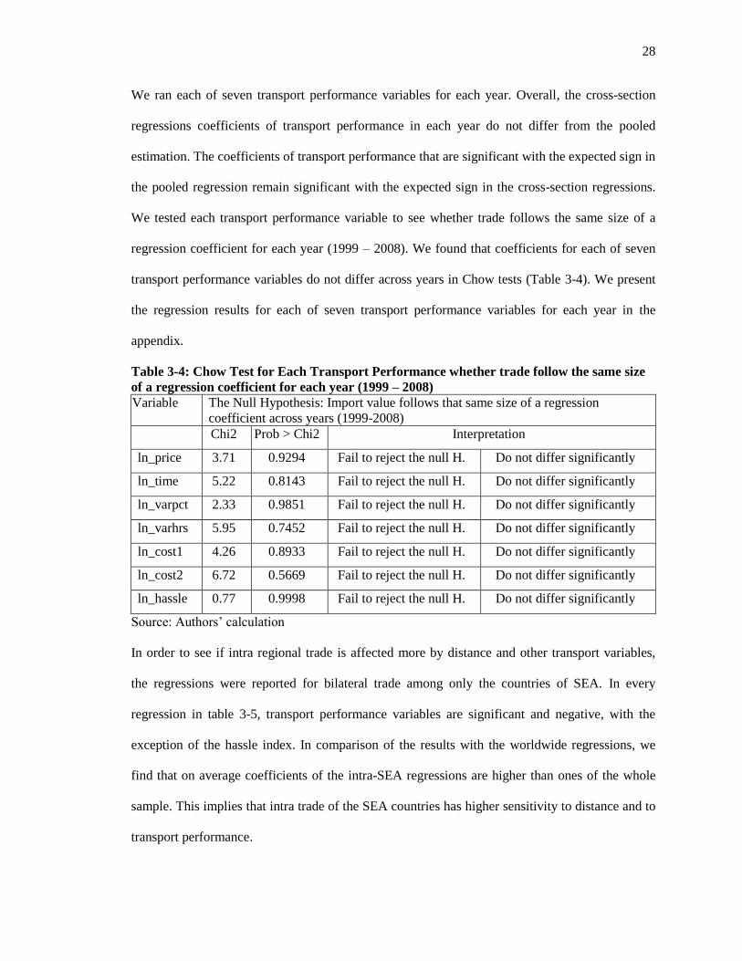
We ran each of seven transport performance variables for each year. Overall, the cross-section

regressions coefficients of transport performance in each year do not differ from the pooled

estimation. The coefficients of transport performance that are significant with the expected sign in

the pooled regression remain significant with the expected sign in the cross-section regressions.

We tested each transport performance variable to see whether trade follows the same size of a

regression coefficient for each year (1999 – 2008). We found that coefficients for each of seven

transport performance variables do not differ across years in Chow tests (Table 3-4). We present

the regression results for each of seven transport performance variables for each year in the

appendix.

Table 3-4: Chow Test for Each Transport Performance whether trade follow the same size

of a regression coefficient for each year (1999 – 2008)

Variable The Null Hypothesis: Import value follows that same size of a regression

coefficient across years (1999-2008)

Chi2 Prob > Chi2 Interpretation

ln_price 3.71 0.9294 Fail to reject the null H. Do not differ significantly

ln_time 5.22 0.8143 Fail to reject the null H. Do not differ significantly

ln_varpct 2.33 0.9851 Fail to reject the null H. Do not differ significantly

ln_varhrs 5.95 0.7452 Fail to reject the null H. Do not differ significantly

ln_cost1 4.26 0.8933 Fail to reject the null H. Do not differ significantly

ln_cost2 6.72 0.5669 Fail to reject the null H. Do not differ significantly

ln_hassle 0.77 0.9998 Fail to reject the null H. Do not differ significantly

Source: Authors‘ calculation

In order to see if intra regional trade is affected more by distance and other transport variables,

the regressions were reported for bilateral trade among only the countries of SEA. In every

regression in table 3-5, transport performance variables are significant and negative, with the

exception of the hassle index. In comparison of the results with the worldwide regressions, we

find that on average coefficients of the intra-SEA regressions are higher than ones of the whole

sample. This implies that intra trade of the SEA countries has higher sensitivity to distance and to

transport performance.

29

Table 3-5: Gravity model regression with measures of transport performance (SEA 1999-2008)

Distance Transport

price

Transport

time

Variability

in percent

Variability

in hours

Cost 1 Cost 2 Hassle

Index

Importer‘s

Population

-3.611**

(1.275)

-1.907

(1.378)

-3.184*

(1.368)

-2.544

(1.337)

-3.343*

(1.370)

-2.207

(1.362)

-2.308

(1.357)

-2.614*

(1.273)

Importer‘s GDP 0.619***

(0.152)

0.434*

(0.172)

0.531***

(0.156)

0.431**

(0.163)

0.551***

(0.154)

0.477**

(0.167)

0.490**

(0.165)

0.472**

(0.172)

Exporter‘s

Population

6.775**

(2.120)

7.579**

(2.437)

6.941**

(2.403)

7.393**

(2.516)

6.715**

(2.404)

7.383**

(2.415)

7.285**

(2.409)

6.737**

(2.277)

Exporter‘s GDP 0.573*

(0.272)

0.544

(0.283)

0.525*

(0.263)

0.504

(0.300)

0.529*

(0.261)

0.546*

(0.275)

0.548*

(0.273)

0.580*

(0.295)

Language -2.739***

(0.390)

-1.129***

(0.244)

-1.367***

(0.200)

-1.525***

(0.291)

-1.266***

(0.204)

-1.100***

(0.227)

-1.072***

(0.227)

-1.697***

(0.269)

Adjacency 0.327*

(0.134)

1.039***

(0.135)

0.940***

(0.126)

0.940***

(0.107)

0.788***

(0.122)

1.064***

(0.126)

1.053***

(0.125)

1.177***

(0.137)

Importer‘s Tariff 0.204*

(0.0999)

0.266**

(0.103)

0.219*

(0.0987)

0.231*

(0.0995)

0.207*

(0.0971)

0.258*

(0.102)

0.254*

(0.102)

0.218*

(0.105)

Importer

Landlocked

-3.577**

(1.386)

-1.143

(1.459)

-4.654**

(1.536)

-1.446

(1.447)

-4.370**

(1.518)

-1.992

(1.461)

-2.144

(1.458)

-2.930

(1.971)

COMESA -1.322***

(0.228)

0.169

(0.277)

-0.0257

(0.252)

0.395

(0.211)

0.351

(0.257)

0.0578

(0.260)

0.0826

(0.259)

-0.0908

(0.223)

EAC 0.958***

(0.230)

1.986***

(0.250)

1.214***

(0.229)

2.663***

(0.282)

1.513***

(0.241)

1.763***

(0.238)

1.755***

(0.237)

2.189***

(0.244)

SACU -4.456***

(0.621)

-3.938***

(0.552)

-3.970***

(0.502)

-4.075***

(0.546)

-4.027***

(0.485)

-3.864***

(0.545)

-3.848***

(0.543)

-3.999***

(0.555)

SADC 0.173

(0.137)

0.308

(0.163)

0.0198

(0.144)

0.213

(0.149)

-0.0294

(0.141)

0.220

(0.160)

0.192

(0.159)

0.394*

(0.159)

Distance -1.429***

(0.124)

Transport Price -0.574***

(0.112)

Transport Time -1.259***

(0.139)

Variability in

percent

-2.331***

(0.345)

Variability in

hours

-1.205***

(0.121)

Cost 1 -0.891***

(0.132)

Cost 2 -0.938***

(0.128)

Hassle Index 2.115

(2.966)

Constant 9.178

(5.667)

-6.812

(7.374)

2.121

(6.447)

4.807

(7.862)

3.809

(6.401)

-2.270

(7.095)

-1.204

(7.018)

-17.30

(15.07)

Number of Obs. 2310 2100 2100 2100 2100 2100 2100 2310

Pseudo R-sq 0.901 0.893 0.904 0.893 0.907 0.897 0.899 0.882

IMPORTER – FIXED EFFECT, EXPORTER – FIXED EFFECT and TIME FIXED EFFECT

Standard errors in parentheses *p<0.05, **p<0.01 and ***p<0.001

30

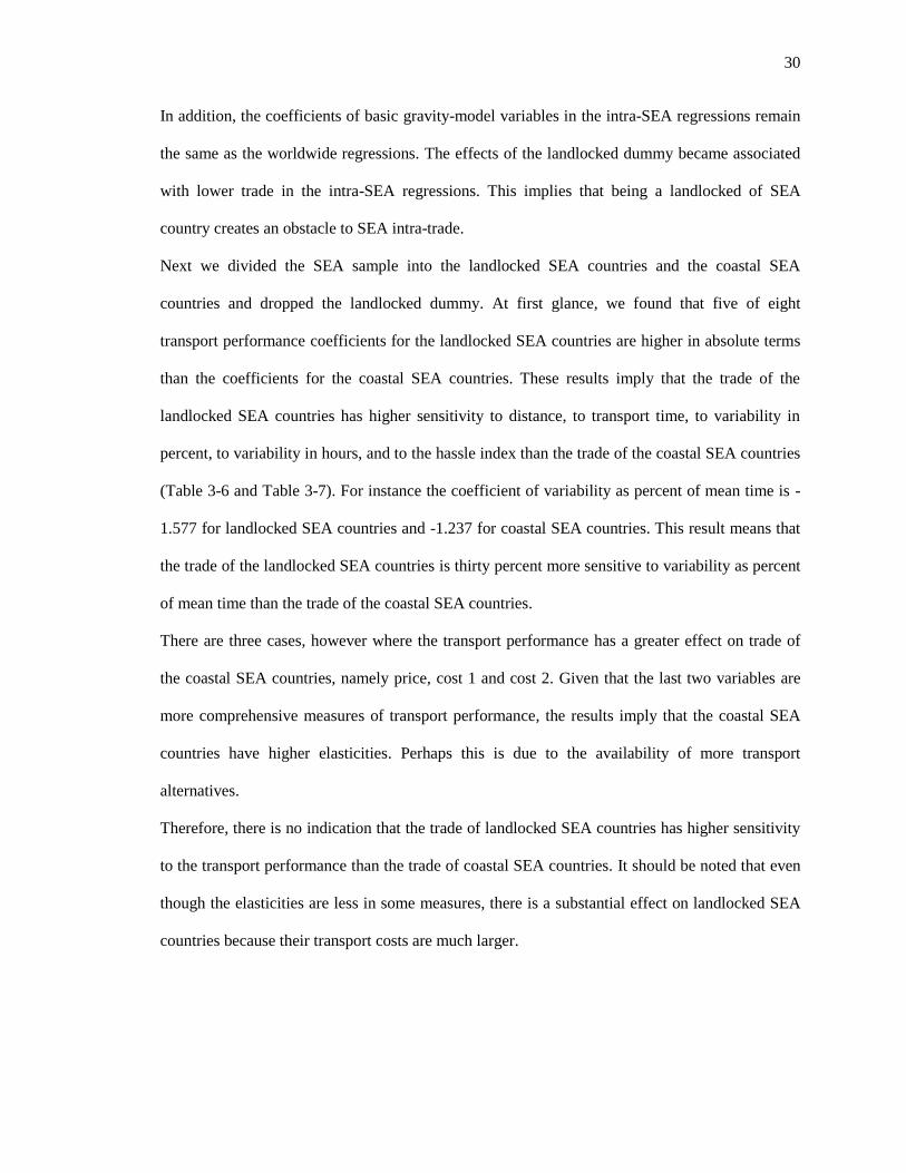
In addition, the coefficients of basic gravity-model variables in the intra-SEA regressions remain

the same as the worldwide regressions. The effects of the landlocked dummy became associated

with lower trade in the intra-SEA regressions. This implies that being a landlocked of SEA

country creates an obstacle to SEA intra-trade.

Next we divided the SEA sample into the landlocked SEA countries and the coastal SEA

countries and dropped the landlocked dummy. At first glance, we found that five of eight

transport performance coefficients for the landlocked SEA countries are higher in absolute terms

than the coefficients for the coastal SEA countries. These results imply that the trade of the

landlocked SEA countries has higher sensitivity to distance, to transport time, to variability in

percent, to variability in hours, and to the hassle index than the trade of the coastal SEA countries

(Table 3-6 and Table 3-7). For instance the coefficient of variability as percent of mean time is -

1.577 for landlocked SEA countries and -1.237 for coastal SEA countries. This result means that

the trade of the landlocked SEA countries is thirty percent more sensitive to variability as percent

of mean time than the trade of the coastal SEA countries.

There are three cases, however where the transport performance has a greater effect on trade of

the coastal SEA countries, namely price, cost 1 and cost 2. Given that the last two variables are

more comprehensive measures of transport performance, the results imply that the coastal SEA

countries have higher elasticities. Perhaps this is due to the availability of more transport

alternatives.

Therefore, there is no indication that the trade of landlocked SEA countries has higher sensitivity

to the transport performance than the trade of coastal SEA countries. It should be noted that even

though the elasticities are less in some measures, there is a substantial effect on landlocked SEA

countries because their transport costs are much larger.

31

Table 3-6: Gravity model regression with measures of transport performance (landlocked SEA 1999-2008)

Distance Transpor

t price

Transport

time

Variability

in percent

Variabilit

y in hours

Cost 1 Cost 2 Hassle

Index

Importer‘s

Population

-2.286

(1.536)

-0.720

(1.700)

-1.445

(1.701)

-1.003

(1.682)

-1.532

(1.708)

-0.768

(1.698)

-0.807

(1.697)

-1.509

(1.496)

Importer‘s GDP 0.731***

(0.184)

0.494*

(0.210)

0.534**

(0.195)

0.485*

(0.200)

0.541**

(0.191)

0.527*

(0.205)

0.535**

(0.204)

0.605**

(0.211)

Exporter‘s

Population

6.556*

(2.739)

7.153*

(3.427)

6.578

(3.417)

7.085*

(3.583)

6.523

(3.470)

6.785*

(3.415)

6.697*

(3.413)

7.186*

(2.935)

Exporter‘s GDP 0.201

(0.252)

0.107

(0.291)

0.109

(0.298)

0.0726

(0.276)

0.103

(0.289)

0.123

(0.297)

0.127

(0.298)

0.258

(0.275)

Language -0.470**

(0.173)

-0.544

(0.321)

-0.207

(0.233)

-0.602*

(0.285)

-0.212

(0.234)

-0.121

(0.286)

-0.0557

(0.276)

-1.043***

(0.306)

Adjacency -0.0293

(0.140)

1.263***

(0.148)

0.912***

(0.147)

1.176***

(0.114)

0.781***

(0.143)

1.191***

(0.150)

1.167***

(0.150)

1.234***

(0.142)

Importer‘s Tariff 0.0941

(0.135)

0.324*

(0.153)

0.228

(0.143)

0.306*

(0.145)

0.213

(0.142)

0.303*

(0.150)

0.296*

(0.149)

0.222

(0.150)

COMESA -1.631***

(0.270)

0.381

(0.290)

0.200

(0.266)

0.690***

(0.208)

0.536

(0.276)

0.267

(0.284)

0.279

(0.283)

0.0875

(0.233)

EAC 0.343

(0.258)

1.627***

(0.334)

0.309

(0.322)

1.923***

(0.290)

0.267

(0.299)

1.036**

(0.347)

0.889*

(0.351)

1.797***

(0.284)

SACU

SADC -0.198

(0.157)

0.161

(0.199)

-0.0838

(0.177)

0.109

(0.191)

-0.115

(0.175)

0.755

(0.193)

0.0536

(0.191)

0.253

(0.205)

Distance -2.125***

(0.160)

Transport Price -0.273**

(0.105)

Transport Time -1.038***

(0.136)

Variability in

percent

-1.577**

(0.550)

Variability in

hours

-1.071***

(0.117)

Cost 1 -

0.710***

(0.131)

Cost 2 -

0.796***

(0.137)

Hassle Index -15.48***

(3.860)

Constant 6.500

(5.837)

-12.61

(8.230)

-7.305

(7.404)

-4.648

(10.40)

-5.670

(7.469)

-8.583

(8.035)

-7.610

(7.972)

73.86***

(20.24)

Number of Obs. 1386 1260 1260 1260 1260 1260 1260 1386

Pseudo R-sq 0.933 0.906 0.917 0.908 0.918 0.910 0.911 0.905

IMPORTER – FIXED EFFECT, EXPORTER – FIXED EFFECT and TIME FIXED EFFECT

Standard errors in parentheses *p<0.05, **p<0.01 and ***p<0.001

32

Table 3-7: Gravity model regression with measures of transport performance (Coastal SEA 1999-

2008) Distance Transport

price

Transport

time

Variability

in percent

Variabilit

y in hours

Cost 1 Cost 2 Hassle

Index

Importer‘s

Population

-11.67***

(3.001)

-11.03***

(3.073)

-11.03***

(3.073)

-10.63***

(3.028)

-10.95***

(3.063)

-10.75***

(3.029)

-10.77***

(3.030)

-11.62***

(3.012)

Importer‘s GDP 0.547**

(0.184)

0.511**

(0.196)

0.511**

(0.196)

0.461*

(0.197)

0.507**

(0.195)

0.486*

(0.192)

0.490*

(0.192)

0.534**

(0.182)

Exporter‘s

Population

0.140

(2.290)

1.229

(2.377)

1.229

(2.377)

1.476

(2.367)

1.172

(2.379)

1.841

(2.338)

1.750

(2.345)

0.178

(2.299)

Exporter‘s GDP 1.086***

(0.258 )

0.999***

(0.261)

0.999***

(0.261)

0.987***

(0.257)

1.000***

(0.258)

0.974***

(0.255)

0.978***

(0.255)

1.092***

(0.259)

Language -1.354***

(0.299)

-0.887**

(0.271)

-1.244***

(0.266)

-1.067***

(0.260)

-1.148***

(0.264)

-1.047***

(0.265)

-1.036***

(0.264)

-1.206***

(0.262)

Adjacency 0.996***

(0.204)

0.975***

(0.167)

0.951***

(0.165)

1.131***

(0.179)

0.926***

(0.159)

0.907***

(0.162)

0.907***

(0.159)

1.211***

(0.198)

Importer‘s

Tariff

0.0786

(0.112)

0.0987

(0.112)

0.100

(0.114)

0.101

(0.113)

0.0989

(0.113)

0.098***

(0.113)

0.0975

(0.112)

0.0774

(0.112)

COMESA -0.806*

(0.346)

0.145

(0.267)

0.142

(0.300)

-0.0862

(0.243)

0.283

(0.292)

0.182

(0.273)

0.213

(0.272)

-0.172

(0.255)

EAC 3.063***

(0.473)

3.396***

(0.367)

3.260***

(0.406)

3.944***

(0.376)

3.461***

(0.389)

3.320***

(0.378)

3.362***

(0.377)

3.873***

(0.348)

SACU -3.498***

(0.714)

-3.631***

(0.740)

-3.783***

(0.727)

-3.724***

(0.797)

-3.830***

(0.748)

-3.693***

(0.742)

-3.721***

(0.749)

-3.581***

(0.756)

SADC -0.306*

(0.142)

-0.315*

(0.143)

-0.406**

(0.152)

-0.323*

(0.148)

-0.398**

(0.151)

-0.362*

(0.147)

-0.370*

(0.147)

-0.271

(0.139)

Distance -0.529*

(0.243)

Transport Price -1.076***

(0.187)

Transport Time -0.990***

(0.177)

Variability in

percent

-1.237***

(0.429)

Variability in

hours

-0.868***

(0.157)

Cost 1 -1.267***

(0.203)

Cost 2 -1.242***

(0.197)

Hassle Index 10.16**

(3.250)

Constant 44.37***

(12.65)

42.77**

(13.22)

43.32**

(13.30)

42.77**

(13.46)

43.18**

(13.27)

46.51***

(13.30)

46.71***

(13.29 )

-12.98

(20.48)

Number of Obs. 924 840 840 840 840 840 840 924

Pseudo R-sq 0.940 0.946 0.945 0.944 0.945 0.946 0.946 0.941

IMPORTER – FIXED EFFECT, EXPORTER – FIXED EFFECT and TIME FIXED EFFECT

Standard errors in parentheses *p<0.05, **p<0.01 and ***p<0.001

33

3.7 Conclusion

This chapter studies the effect of new measures of transport performance on international trade

among 15 counties in southern and eastern Africa and on the international trade of those countries

with six other regions in the world. The RESET test indicates estimates with country and time

fixed effects performed better in terms of explained variance. We find that most of the transport

variables and distance have similar negative effects on trade. The results indicate that a 10 percent

reduction in transport costs increases trade volumes by about 10 percent. Our results are

substantially smaller in absolute terms to those found elsewhere in the literatures. We also find

that coefficients for each of seven transport performance measures do not differ significantly

across years

The PPML estimator indicates that intra-regional trade of the SEA countries has higher sensitivity

to distance and to transport performance than the worldwide trade. In addition we find that that

being landlocked of SEA countries show an obstacle to SEA intra-trade but there is no indication

that the trade of landlocked SEA countries has higher sensitivity to the transport performance

than the trade of coastal SEA countries.

34

3.8 Appendix

Table A3-1: Regression with measures of transport performance (Panel 1999-2008) _NO FIXED EFFECT

Distance Transport

price

Transport

time

Variability

in percent

Variability

in hours

Cost 1 Cost 2 Hassle

Index

Importer‘s

Population

-0.171***

(0.0483)

-0.172***

(0.0562)

0.045

(0.0606)

0.042

(0.0582)

0.005

(0.0589)

0.012

(0.0606)

-0.113*

(0.0565)

-0.188***

(0.0467)

Importer‘s GDP 0.851***

(0.0304)

0.994***

(0.0293)

0.843***

(0.0367)

0.882***

(0.0355)

0.829***

(0.0362)

0.899***

(0.0345)

0.885***

(0.0304)

1.042***

(0.0403)

Exporter‘s

Population

0.221***

(0.0382)

-0.029

(0.0578)

0.073

(0.0623)

0.020

(0.0563)

0.0072

(0.0568)

0.074

(0.0639)

-0.004

(0.0566)

0.165***

(0.0453)

Exporter‘s GDP 0.697***

(0.0246)

0.964***

(0.2788)

0.858***

(0.0312)

0.888***

(0.0322)

0.832***

(0.0323)

0.896***

(0.0285)

0.871***

(0.0271)

0.907***

(0.0424)

Language -0.566***

(0.0673)

0.227

(0.1066)

-0.356**

(0.1117)

0.033

(0.1239)

-0.022

(0.1205)

-0.280*

(0.1152)

-0.137

(0.1097)

0.364***

(0.1026)

Adjacency -0.807***

(0.1643)

2.388***

(0.3630)

1.480***

(0.2505)

2.753***

(0.3892)

2.123***

(0.2982)

1.368***

(0.1728)

1.714***

(0.2406)

-0.072

(0.1336)

Importer‘s Tariff -0.059

(0.0547)

0.031

(0.0602)

0.005

(0.0713)

0.015

(0.0712)

-0.017

(0.0687)

0.001

(0.0652)

-0.002

(0.0582)

-0.082

(0.0719)

Importer

Landlocked

-0.914***

(0.1152)

0.113

(0.0882)

-0.054

(0.0893)

-0.058

(0.0988)

0.025

(0.0918)

0.192*

(0.0862)

0.169*

(0.0817)

-0.502**

(0.1452)

COMESA -0.213

(0.2013)

0.137

(0.2078)

-0.245

(0.1909)

-0.085

(0.2496)

0.013

(0.1922)

-0.594**

(0.2047)

-0.336

(0.2055)

0.409

(0.2753)

EAC 1.890***

(0.2969)

1.903***

(0.4108)

1.104***

(0.2832)

1.989***

(0.4806)

1.484***

(0.3526)

1.331***

(0.2303)

1.789***

(0.2669)

4.139***

(0.3514)

SACU -5.308***

(0.5598)

-6.081***

(0.5300)

-6.199***

(0.5191)

-6.269***

(0.5353)

-6.269***

(0.5267)

-5.889***

(0.5304)

-6.051***

(0.5182)

-4.568***

(0.5767)

SADC -0.949***

(0.2043)

1.554***

(0.3784)

0.889***

(0.2685)

1.868***

(0.4113)

1.298***

(0.3265)

0.252

(0.1790)

0.894***

(0.2589)

3.141***

(0.2177)

Distance -1.00***

(0.0770)

Transport Price -0.747***

(0.0563)

Transport Time -1.141***

(0.0933)

Variability in

percent

-0.313***

(0.0571)

Variability in

hours

-0.459***

(0.0519)

Cost 1 -1.220***

(0.0722)

Cost 2 -1.204***

(0.0766)

Hassle Index 0.923***

(0.1417)

Constant 6.804***

(0.7249)

2.317***

(0.6622)

4.056***

(0.7017)

-2.576***

(0.5537)

0.137

(0.6204)

8.853***

(0.7085)

8.491***

(0.8499)

-8.899***

(1.0514)

Number of Obs. 4620 3900 3900 3900 3900 3900 3900 4620

Pseudo R-sq 0.971 0.866 0.8710 0.8476 0.8616 0.8788 0.8802 0.9647

RESET p-val. 0.0000 0.0000 0.0000 0.0000 0.0031 0.0296 0.2336 0.4650 NO IMPORTER – FIXED EFFECT, NO EXPORTER – FIXED EFFECT and NO TIME FIXED EFFECT

Standard errors in parentheses *p<0.05, **p<0.01 and ***p<0.001

35

Table A3-2: Gravity model regression with Transport Price on Cross Section

1999 2000 2001 2002 2003 2004 2005 2006 2007 2008

Importer‘s

Population

-1.437**

(0.437)

-0.502

(0.798)

1.472

(8.679)

0.423

(1.323)

-0.751

(0.904)

-0.744

(0.961)

-0.269

(0.776)

0.244

(0.570)

-0.126

(0.490)

0.427

(0.567)

Importer‘s GDP 1.744*

(0.802)

0.679

(1.166)

-2.863

(14.97)

-0.845

(1.230)

1.275

(0.801)

1.600

(1.256)

0.955

(1.061)

0.418

(0.594)

0.728

(0.425)

0.351

(0.403)

Exporter‘s

Population

-1.335

(0.975)

-1.413

(0.799)

6.066

(6.660)

0.353

(0.892)

-0.174

(0.622)

-0.740

(0.760)

-1.638*

(0.738)

-1.146*

(0.532)

-1.356*

(0.559)

-0.671

(0.497)

Exporter‘s GDP 1.480*

(0.689)

1.383

(0.847)

-12.14

(12.01)

-1.042

(0.973)

-0.224

(0.553)

0.259

(1.185)

0.990

(0.653)

0.786*

(0.356)

0.522

(0.354)

0.548*

(0.266)

Language -0.222

(0.387)

-0.253

(0.332)

0.322

(0.406)

0.0398

(0.314)

0.00826

(0.375)

0.107

(0.367)

0.00449

(0.382)

-0.0533

(0.372)

0.00205

(0.355)

0.053

(0.294)

Adjacency 0.893

(0.473)

1.765***

(0.492)

1.767***

(0.502)

2.032***

(0.431)

2.106***

(0.421)

1.918***

(0.435)

1.841***

(0.529)

2.012***

(0.570)

1.926***

(0.484)

1.853***

(0.474)

Importer‘s Tariff 0.644

(0.452)

0.315

(0.617)

0.0173

(0.356)

-0.0966

(0.514)

-0.00213

(0.314)

0.0668

(0.659)

-0.325

(0.532)

1.173

(0.893)

-0.667

(0.703)

1.773*

(0.903)

Importer

Landlocked

0.230

(0.468)

0.344

(0.886)

-1.141

(5.886)

-0.341

(0.474)

0.448

(0.391)

0.581

(0.502)

0.456

(0.441)

0.392

(0.304)

0.301

(0.295)

0.364

(0.250)

COMESA 0.524

(0.387)

-0.0065

(0.421)

-0.305

(0.455)

0.112

(0.425)

0.400

(0.429)

0.136

(0.397)

0.620

(0.626)

0.296

(0.625)

-0.558

(0.502)

-0.666

(0.510)

EAC 2.979***

(0.756)

2.214**

(0.744)

2.512***

(0.748)

1.735*

(0.703)

1.390*

(0.628)

1.625*

(0.707)

1.630*

(0.795)

1.680*

(0.818)

2.049**

(0.693)

2.274**

(0.746)

SACU -9.776***

(0.733)

-6.734***

(1.302)

-6.979***

(1.419)

-6.833***

(1.308)

-6.496***

(1.301)

-6.656***

(1.326)

-6.034***

(1.274)

-5.185***

(1.285)

SADC 0.240

(0.508)

-0.700

(0.624)

-0.0276

(0.593)

-0.415

(0.531)

-0.684

(0.691)

0.644

(0.412)

0.607

(0.437)

0.690

(0.487)

0.338

(0.374)

0.530

(0.421)

Transport Price -0.690***

(0.203)

-0.591**

(0.194)

-0.659***

(0.175)

-0.641***

(0.162)

-0.718***

(0.168)

-0.625***

(0.186)

-0.791**

(0.243)

-0.742***

(0.223)

-0.655**

(0.249)

-0.7688***

(0.190)

Constant 7.292*

(3.253)

6.701

(4.961)

8.648

(5.032)

7.032*

(3.305)

7.232**

(2.611)

5.793

(3.453)

9.226*

(4.012)

3.568

(4.516)

9.775*

(4.275)

1.452

(4.002)

Number of Obs. 390 390 390 390 390 390 390 390 390 390

Pseudo R-sq 0.951 0.943 0.939 0.941 0.938 0.941 0.931 0.928 0.937 0.939

IMPORTER – FIXED EFFECT, EXPORTER – FIXED EFFECT and TIME FIXED EFFECT

The Null Hypothesis: Import value follows that same size of a regression coefficient across years (1999-2008)

Chi2 = 3.71, Prob > Chi2 = 0.9294, and Fail to reject the null Hypothesis.

Standard errors in parentheses *p<0.05, **p<0.01 and ***p<0.001

3

5

36

Table A3-3: Gravity model regression with Transport Time on Cross Section

1999 2000 2001 2002 2003 2004 2005 2006 2007 2008

Importer‘s

Population

-1.543***

(0.319)

-0.00935

(0.837)

-2.804

(7.926)

-0.198

(1.219)

-1.322

(0.819)

-1.328

(0.899)

-0.600

(0.694)

0.126

(0.503)

-0.243

(0.401)

0.307

(0.456)

Importer‘s GDP 1.393*

(0.655)

-0.0128

(1.142)

4.502

(13.67)

-0.208

(1.167)

1.819*

(0.760)

2.717*

(1.166)

1.698

(1.083)

0.898

(0.534)

1.120**

(0.383)

0.752*

(0.306)

Exporter‘s

Population

-1.339

(0.934)

-1.295

(0.816)

5.124

(6.795)

0.204

(0.854)

-0.337

(0.625)

-0.954

(0.781)

-1.500*

(0.732)

-1.129*

(0.529)

-1.175*

(0.549)

-0.622

(0.488)

Exporter‘s GDP 1.479*

(0.732)

1.215

(0.884)

-10.37

(12.34)

-0.893

(0.984)

0.190

(0.625)

0.562

(1.257)

1.409

(0.737)

0.955**

(0.359)

0.730*

(0.336)

0.681**

(0.230)

Language -0.824

(0.511)

-0.785*

(0.381)

-0.225

(0.493)

-0.576

(0.362)

-0.748

(0.473)

-0.386

(0.434)

-0.761

(0.431)

-0.710

(0.407)

-0.593

(0.380)

-0.517

(0.297)

Adjacency 0.248

(0.442)

1.190*

(0.464)

1.293**

(0.481)

1.514***

(0.394)

1.677***

(0.369)

1.750***

(0.425)

1.563***

(0.462)

1.679***

(0.480)

1.542***

(0.416)

1.272***

(0.383)

Importer‘s Tariff 0.561

(0.396)

0.725

(0.674)

0.151

(0.339)

0.142

(0.596)

0.299

(0.304)

0.328

(0.768)

0.0226

(0.480)

1.312

(0.850)

-0.400

(0.593)

2.308*

(0.924)

Importer

Landlocked

-0.868*

(0.353)

-0.288

(0.825)

1.006

(5.361)

-0.921*

(0.375)

-0.236

(0.338)

0.341

(0.439)

-0.0439

(0.418)

-0.173

(0.297)

-0.213

(0.235)

-0.128

(0.247)

COMESA -0.0237

(0.397)

-0.471

(0.445)

-0.574

(0.418)

-0.247

(0.416)

-0.0269

(0.419)

-0.128

(0.419)

0.237

(0.592)

0.0167

(0.548)

-0.809*

(0.403)

-0.909*

(0.402)

EAC 2.752***

(0.515)

2.023***

(0.532)

2.169***

(0.554)

1.470**

(0.503)

1.092*

(0.527)

1.049

(0.621)

0.877

(0.744)

0.875

(0.811)

1.263

(0.671)

1.469

(0.777)

SACU -9.561***

(0.822)

-6.614***

(1.327)

-7.043***

(1.421)

-6.918***

(1.324)

-6.703***

(1.314)

-6.823***

(1.334)

-6.148***

(1.237)

-5.229***

(1.238)

SADC -0.0318

(0.460)

-0.836

(0.575)

-0.144

(0.536)

-0.526

(0.479)

-0.691

(0.598)

0.393

(0.406)

0.402

(0.418)

0.476

(0.471)

0.117

(0.331)

0.430

(0.387)

Transport Time -1.128***

(0.192)

-1.008***

(0.199)

-0.857***

(0.241)

-0.948***

(0.187)

-1.024***

(0.200)

-0.776***

(0.217)

-1.081***

(0.227)

-1.104***

(0.232)

-1.086***

(0.237)

-1.308***

(0.184)

Constant 10.72***

(2.585)

7.394

(4.805)

6.598

(4.549)

8.505**

(3.067)

8.191***

(2.376)

4.615

(3.405)

7.329*

(3.544)

3.269

(3.829)

9.389**

(3.382)

1.004

(3.604)

Number of Obs. 390 390 390 390 390 390 390 390 390 390

Pseudo R-sq 0.956 0.949 0.942 0.945 0.942 0.943 0.935 0.934 0.943 0.950

IMPORTER – FIXED EFFECT, EXPORTER – FIXED EFFECT and TIME FIXED EFFECT

The Null Hypothesis: Import value follows that same size of a regression coefficient across years (1999-2008)

Chi2 = 5.22 , Prob > Chi2 = 0.8143 , and Fail to reject the null Hypothesis.

Standard errors in parentheses *p<0.05, **p<0.01 and ***p<0.001 36

37

Table A3-4: Gravity model regression with Variability in percent on Cross Section

1999 2000 2001 2002 2003 2004 2005 2006 2007 2008

Importer‘s

Population

-1.312**

(0.465)

-0.423

(0.774)

-0.951

(9.211)

0.132

(1.394)

-0.999

(1.014)

-0.839

(1.129)

-0.214

(0.976)

0.272

(0.689)

-0.0212

(0.604)

0.366

(0.632)

Importer‘s GDP 1.451

(0.880)

0.369

(1.190)

1.369

(15.83)

-0.628

(1.281)

1.404

(0.829)

1.752

(1.404)

0.857

(1.370)

0.342

(0.732)

0.648

(0.514)

0.377

(0.451)

Exporter‘s

Population

-1.275

(0.858)

-1.706**

(0.644)

5.505

(6.267)

0.280

(0.913)

-0.223

(0.612)

-0.700

(0.836)

-1.332

(0.814)

-1.183*

(0.526)

-1.115

(0.598)

-0.809

(0.461)

Exporter‘s GDP 1.305*

(0.660)

1.549*

(0.751)

-11.22

(11.19)

-1.254

(0.935)

-0.224

(0.553)

-0.0198

(1.217)

-0.895

(0.769)

0.708

(0.392)

0.492

(0.357)

-0.506*

(0.250)

Language -0.520

(0.488)

-0.508

(0.384)

-0.0421

(0.486)

-0.298

(0.394)

-0.411

(0.482)

-0.144

(0.432)

-0.493

(0.432)

-0.487

(0.411)

-0.450

(0.375)

-0.372

(0.318)

Adjacency 1.318**

(0.439)

2.046***

(0.468)

2.181***

(0.486)

2.325***

(0.425)

2.459***

(0.430)

2.251***

(0.476)

2.334***

(0.560)

2.479***

(0.585)

2.337***

(0.490)

2.256***

(0.464)

Importer‘s Tariff 0.868

(0.484)

0.317

(0.582)

0.265

(0.411)

-0.0718

(0.542)

0.240

(0.382)

0.250

(0.687)

-0.0235

(0.604)

1.210

(0.868)

-0.297

(0.781)

1.524

(0.830)

Importer

Landlocked

-0.320

(0.516)

-0.170

(0.875)

0.0416

(6.227)

-0.758

(0.503)

-0.0642

(0.423)

0.202

(0.539)

-0.0309

(0.528)

-0.103

(0.363)

-0.0246

(0.290)

-0.00847

(0.289)

COMESA 0.399

(0.474)

-0.255

(0.537)

-0.580

(0.599)

-0.159

(0.548)

0.0437

(0.581)

-0.219

(0.648)

0.0644

(0.851)

-0.249

(0.847)

-1.008

(0.676)

-1.239

(0.710)

EAC 2.493**

(0.850)

2.073*

(0.860)

2.256*

(0.908)

1.587

(0.857)

1.263

(0.806)

1.580

(0.859)

1.640

(1.014)

1.725

(1.028)

2.212*

(0.862)

2.623**

(0.878)

SACU -9.662***

(0.698)

-6.651***

(1.283)

-6.762***

(1.411)

-6.807***

(1.297)

-6.590***

(1.276)

-6.716***

(1.301)

-6.162***

(1.279)

-5.239***

(1.266)

SADC 0.0921

(0.521)

-0.711

(0.601)

-0.0849

(0.608)

-0.405

(0.519)

-0.765

(0.715)

0.672

(0.448)

0.611

(0.502)

0.673

(0.512)

0.345

(0.445)

0.564

(0.456)

Variability in

percent

-0.0526

(0.159)

-0.0505

(0.170)

0.0752

(0.169)

-0.0370

(0.165)

-0.0490

(0.183)

0.0115

(0.181)

0.0723

(0.179)

0.0642

(0.180)

0.169

(0.193)

0.0871

(0.166)

Constant 1.928

(3.032)

3.290

(5.047)

1.247

(5.193)

3.216

(3.648)

2.143

(3.359)

0.601

(3.578)

1.302

(4.400)

-2.345

(4.384)

1.903

(4.533)

-3.918

(3.687)

Number of Obs. 390 390 390 390 390 390 390 390 390 390

Pseudo R-sq 0.947 0.940 0.935 0.936 0.931 0.937 0.922 0.920 0.932 0.932

IMPORTER – FIXED EFFECT, EXPORTER – FIXED EFFECT and TIME FIXED EFFECT

The Null Hypothesis: Import value follows that same size of a regression coefficient across years (1999-2008)

Chi2 = 2.33 , Prob > Chi2 = 0.9851 , and Fail to reject the null Hypothesis.

Standard errors in parentheses *p<0.05, **p<0.01 and ***p<0.001 37

38

Table A3-5: Gravity model regression with Variability in hours on Cross Section

1999 2000 2001 2002 2003 2004 2005 2006 2007 2008

Importer‘s

Population

-1.623***

(0.399)

-0.199

(0.813)

-1.152

(8.469)

-0.0724

(1.281)

-1.428

(0.883)

-1.291

(0.989)

-0.628

(0.844)

-0.0471

(0.602)

-0.308

(0.528)

0.214

(0.534)

Importer‘s GDP 1.580*

(0.767)

0.244

(1.140)

1.474

(14.55)

-0.531

(1.197)

1.676*

(0.749)

2.345

(1.242)

1.329

(1.218)

0.674

(0.626)

0.950*

(0.456)

0.670

(0.379)

Exporter‘s

Population

-1.682

(0.938)

-1.701*

(0.749)

5.927

(7.062)

0.246

(0.938)

-0.479

(0.622)

-0.996

(0.823)

-1.642*

(0.807)

-1.361*

(0.546)

-1.326*

(0.618)

-0.833

(0.494)

Exporter‘s GDP 1.709*

(0.833)

1.578

(0.893)

-12.08

(12.65)

-1.199

(1.007)

0.0135

(0.603)

0.334

(1.237)

1.173

(0.783)

0.875*

(0.405)

0.689

(0.388)

0.703**

(0.265)

Language -0.397

(0.432)

-0.369

(0.331)

0.090

(0.452)

-0.221

(0.342)

-0.332

(0.425)

-0.121

(0.410)

-0.374

(0.395)

-0.354

(0.387)

-0.270

(0.352)

-0.173

(0.285)

Adjacency 0.662

(0.417)

1.477**

(0.475)

1.695***

(0.509)

1.749***

(0.416)

1.900***

(0.407)

1.935***

(0.432)

1.906***

(0.495)

1.977***

(0.530)

1.941***

(0.473)

1.764***

(0.426)

Importer‘s Tariff 0.542

(0.446)

0.689

(0.645)

0.236

(0.395)

-0.00707

(0.567)

0.261

(0.349)

0.239

(0.723)

-0.0904

(0.601)

1.159

(0.907)

-0.339

(0.812)

1.757

(0.923)

Importer

Landlocked

-0.521

(0.418)

-0.0261

(0.838)

-0.0151

(5.717)

-0.876

(0.448)

-0.221

(0.375)

0.141

(0.481)

-0.357

(0.511)

-0.467

(0.365)

-0.317

(0.312)

-0.409

(0.298)

COMESA 0.242

(0.397)

-0.278

(0.448)

-0.488

(0.490)

-0.0936

(0.433)

0.0465

(0.443)

-0.266

(0.499)

0.0109

(0.708)

-0.302

(0.691)

-1.040

(0.554)

-1.300*

(0.551)

EAC 2.692***

(0.637)

2.132***

(0.640)

2.307**

(0.723)

1.617**

(0.623)

1.304*

(0.578)

1.480*

(0.693)

1.464

(0.853)

1.621

(0.873)

2.076**

(0.724)

2.404**

(0.755)

SACU -9.558***

(0.777)

-6.550***

(1.315)

-6.777***

(1.422)

-6.728***

(1.320)

-6.465***

(1.301)

-6.526***

(1.335)

-5.949***

(1.263)

-4.972***

(1.269)

SADC 0.0259

(0.459)

-0.784

(0.556)

-0.112

(0.548)

-0.479

(0.471)

-0.731

(0.589)

0.558

(0.398)

0.552

(0.424)

0.660

(0.478)

0.396

(0.378)

0.764

(0.428)

Variability in

hours

0.539***

(0.157)

-0.496**

(0.155)

-0.325

(0.185)

-0.478***

(0.145)

-0.501**

(0.165)

-0.339

(0.178)

-0.420*

(0.188)

-0.453*

(0.192)

-0.339

(0.199)

-0.439**

(0.148)

Constant 7.729*

(3.087)

5.089

(4.914)

4.725

(4.849)

6.871*

(3.426)

6.845*

(2.946)

3.814

(3.669)

6.003

(4.455)

2.330

(4.529)

6.158

(4.578)

-1.019

(3.785)

Number of Obs. 390 390 390 390 390 390 390 390 390 390

Pseudo R-sq 0.951 0.945 0.937 0.941 0.937 0.939 0.926 0.925 0.934 0.937

IMPORTER – FIXED EFFECT, EXPORTER – FIXED EFFECT and TIME FIXED EFFECT

The Null Hypothesis: Import value follows that same size of a regression coefficient across years (1999-2008)

Chi2 = 5.95 , Prob > Chi2 = 0.7452 , and Fail to reject the null Hypothesis.

Standard errors in parentheses *p<0.05, **p<0.01 and ***p<0.001 38

39

Table A3-6: Gravity model regression with Cost 1 on Cross Section

1999 2000 2001 2002 2003 2004 2005 2006 2007 2008

Importer‘s

Population

-1.420***

(0.394)

-0.242

(0.822)

-0.271

(8.395)

0.266

(1.284)

-0.915

(0.877)

-0.921

(0.960)

-0.349

(0.744)

0.140

(0.546)

-0.188

(0.449)

0.332

(0.516)

Importer‘s GDP 1.670*

(0.728)

0.450

(1.131)

0.161

(14.47)1

-0.658

(1.204)

1.425

(0.792)

1.940

(1.243)

1.095

(1.047)

0.538

(0.569)

0.806*

(0.399)

0.456

(0.362)

Exporter‘s

Population

-1.289

(0.922)

-1.353

(0.768)

6.479

(6.205)

0.451

(0.816)

-0.0934

(0.563)

-0.638

(0.702)

-1.343

(0.688)

-0.999*

(0.485)

-1.128*

(0.523)

-0.475

(0.473)

Exporter‘s GDP 1.574*

(0.688)

1.446

(0.806)

-12.80

(11.23)

-1.149

(0.921)

-0.172

(0.533)

0.0904

(1.097)

0.963

(0.625)

0.704*

(0.317)

0.473

(0.304)

0.490*

(0.224)

Language -0.629

(0.529)

-0.584

(0.410)

-0.0625

(0.511)

-0.359

(0.399)

-0.486

(0.499)

-0.208

(0.439)

-0.524

(0.428)

-0.515

(0.410)

-0.393

(0.381)

-0.319

(0.301)

Adjacency 0.719

(0.425)

1.577***

(0.469)

1.744***

(0.488)

1.942***

(0.417)

2.047***

(0.409)

1.965***

(0.442)

1.751***

(0.493)

1.887***

(0.530)

1.731***

(0.454)

1.527***

(0.425)

Importer‘s Tariff 0.653

(0.433)

0.512

(0.655)

0.111

(0.359)

-0.00244

(0.582)

0.137

(0.326)

0.290

(0.757)

-0.141

(0.490)

1.175

(0.884)

-0.566

(0.603)

2.113*

(0.931)

Importer

Landlocked

-0.262

(0.412)

0.0681

(0.840)

-0.411

(5.695)

-0.713

(0.433)

0.00492

(0.355)

0.289

(0.480)

0.0356

(0.395)

-0.0659

(0.265)

-0.0735

(0.197)

-0.0036

(0.210)

COMESA 0.00302

(0.403)

-0.417

(0.438)

-0.590

(0.458)

-0.226

(0.432)

0.00390

(0.441)

-0.152

(0.440)

0.233

(0.588)

-0.00267

(0.567)

-0.813*

(0.414)

-0.921*

(0.425)

EAC 2.958***

(0.652)

2.200***

(0.666)

2.273**

(0.711)

1.576*

(0.664)

1.220*

(0.602)

1.332*

(0.677)

1.360

(0.759)

1.445

(0.787)

1.824**

(0.639)

2.228*

(0.731)

SACU -9.580***

(0.732)

-6.568***

(1.298)

-6.812***

(1.407)

-6.767***

(1.309)

-6.415***

(1.292)

-6.524***

|(0.492)

0.264

(0.356)

0.584

(0.426)

SADC 0.141

(0.474)

-0.704

(0.595)

-0.0968

(0.566)

-0.457

(0.512)

-0.733

(0.659)

0.529

(0.411)

0.550

(0.429)

0.640

(0.492)

0.264

(0.356)

0.584

(0.426)

Cost 1 -1.138***

(0.201)

-1.018***

(0.218)

-0.761**

(0.269)

-0.875***

(0.203)

-0.955***

(0.223)

-0.744**

(0.254)

-1.145***

(0.267)

-1.119***

(0.27)

-1.138***

(0.296)

-1.363***

(0.207)

Constant 12.28***

(2.995)

10.31*

(4.983)

9.275

(5.144)

9.891***

(3.356)

10.11***

(2.864)

6.980

(3.956)

12.34**

(3.968)

7.888

(4.754)

14.35***

(4.118)

6.462

(4.234)

Number of Obs. 390 390 390 390 390 390 390 390 390 390

Pseudo R-sq 0.954 0.947 0.939 0.942 0.938 0.941 0.933 0.930 0.941 0.946

IMPORTER – FIXED EFFECT, EXPORTER – FIXED EFFECT and TIME FIXED EFFECT

The Null Hypothesis: Import value follows that same size of a regression coefficient across years (1999-2008)

Chi2 = 5.95 , Prob > Chi2 = 0.7452, and Fail to reject the null Hypothesis.

Standard errors in parentheses *p<0.05, **p<0.01 and ***p<0.001

39

40

Table A3-7: Gravity model regression with Cost 2 on Cross Section

1999 2000 2001 2002 2003 2004 2005 2006 2007 2008

Importer‘s

Population

-1.621***

(0.382)

-0.362

(0.819)

0.0574

(8.186)

0.192

(1.251)

-1.101

(0.841)

-1.107

(0.908)

-0.523

(0.714)

0.0311

(0.521)

-0.290

(0.432)

0.281

(0.492)

Importer‘s GDP 1.808*

(0.702)

0.525

(1.110)

-0.545

(14.12)

-0.682

(1.178)

1.512*

(0.766)

2.126

(1.186)

1.305

(1.015)

0.668

(0.542)

0.927*

(0.380)

0.569

(0.349)

Exporter‘s

Population

-1.449

(0.960)

-1.357

(0.839)

5.946

(6.816)

0.346

(0.867)

-0.274

(0.603)

-0.859

(0.737)

-1.588*

(0.703)

-1.153*

(0.508)

-1.314*

(0.553)

-0.587

(0.496)

Exporter‘s GDP 1.700*

(0.761)

1.393

(0.907)

-11.90

(12.32)

-1.043

(0.995)

-0.0268

(0.583)

0.373

(1.171)

1.171

(0.663)

0.854*

(0.345)

0.629

(0.339)

0.640*

(0.253)

Language -0.376

(0.438)

-0.373

(0.346)

0.103

(0.455)

-0.181

(0.348)

-0.255

(0.422)

-0.0752

(0.398)

-0.245

(0.377)

-0.259

(0.377)

-0.153

(0.348)

-0.0765

(0.278)

Adjacency 0.536

(0.432)

1.478**

(0.473)

1.605**

(0.490)

1.819***

(0.411)

1.925***

(0.399)

1.876***

(0.414)

1.699***

(0.465)

1.809***

(0.509)

1.723***

(0.450)

1.542***

(0.414)

Importer‘s Tariff 0.561

(0.419)

0.529

(0.658)

0.123

(0.357)

-0.0563

(0.561)

0.140

(0.318)

0.192

(0.736)

-0.199

(0.507)

1.136

(0.895)

-0.585

(0.662)

1.952*

(0.937)

Importer

Landlocked

-0.146

(0.379)

0.187

(0.833)

-0.622

(5.557)

-0.657

(0.424)

0.0610

(0.345)

0.288

(0.462)

-0.0964

(0.406)

-0.173

(0.266)

-0.123

(0.222)

-0.292

(0.238)

COMESA 0.0522

(0.413)

-0.313

(0.432)

-0.515

(0.437)

-0.134

(0.416)

0.0654

(0.417)

-0.163

(0.413)

0.213

(0.565)

-0.0577

(0.545)

-0.811*

(0.412)

-1.022*

(0.419)

EAC 3.168***

(0.643)

2.285***

(0.643)

2.395***

(0.676)

1.676**

(0.622)

1.341*

(0.564)

1.434*

(0.653)

1.391

(0.732)

1.527*

(0.760)

1.879**

(0.622)

2.202**

(0.695)

SACU -9.606***

(0.771)

-6.595***

(1.312)

-6.879***

(1.416)

-6.771***

(1.319)

-6.453***

(1.318)

-6.533***

(1.348)

-5.956***

(1.277)

-5.013***

(1.295)

SADC 0.144

(0.475)

-0.745

(0.594)

-0.111

(0.557)

-0.483

(0.503)

-0.737

(0.623)

0.537

(0.392)

0.527

(0.396)

0.632

(0.471)

0.306

(0.337)

0.637

(0.413)

Cost 2 -1.127***

(0.227)

-0.958***

(0.225)

-0.781**

(0.262)

-0.869***

(0.208)

-0.949***

(0.219)

-0.744**

(0.247)

-1.050***

(0.262)

-1.042***

(0.268)

-0.976**

(0.302)

-1.181***

(0.215)

Constant 12.97***

(3.278)

9.997*

(5.009)

9.991

(5.164)

10.40**

(3.377)

10.78***

(2.911)

7.682

(4.002)

12.26**

(4.118)

7.722

(4.802)

13.29**

(4.472)

5.583

(4.346)

Number of Obs. 390 390 390 390 390 390 390 390 390 390

Pseudo R-sq 0.954 0.947 0.940 0.943 0.939 0.941 0.934 0.931 0.940 0.944

IMPORTER – FIXED EFFECT, EXPORTER – FIXED EFFECT and TIME FIXED EFFECT

The Null Hypothesis: Import value follows that same size of a regression coefficient across years (1999-2008)

Chi2 = 0.77, Prob > Chi2 = 0.9998 , and Fail to reject the null Hypothesis.

Standard errors in parentheses *p<0.05, **p<0.01 and ***p<0.001

40

41

Table A3-8: Gravity model regression with Hassle Index on Cross Section

1999 2000 2001 2002 2003 2004 2005 2006 2007 2008

Importer‘s

Population

-0.580

(0.859)

0.853

(0.995)

3.558

(9.265)

0.783

(1.235)

-0.343

(1.005)

0.0756

(0.898)

0.217

(0.768)

0.285

(0.583)

0.197

(0.539)

0.334

(0.535)

Importer‘s GDP 1.334

(1.040)

0.151

(1.215)

-6.474

(16.34)

-1.029

(1.208)

1.183

(0.885)

0.868

(1.374)

0.668

(1.056)

0.175

(0.573)

0.461

(0.454)

0.198

(0.405)

Exporter‘s

Population

-2.020

(1.321)

-1.518

(0.995)

12.78

(7.650)

0.951

(1.213)

0.185

(0.913)

0.226

(0.899)

-0.718

(0.926)

-0.873

(0.676)1

-0.482

(0.650)

-0.518

(0.551)

Exporter‘s GDP 2.381*

(1.130)

1.992

(1.044)

-24.56

(13.66)

-2.043

(1.066)

-0.960

(0.681)

-0.939

(1.142)

0.630

(0.856)

0.422

(0.442)

0.407

(0.402)

0.311

(0.279)

Language 0.424

(0.218)

0.305

(0.212)

0.477*

(0.220)

0.309

(0.216)

0.239

(0.210)

0.340

(0.195)

0.408*

(0.177)

0.430*

(0.196)

0.470*

(0.196)

0.520*

(0.207)

Adjacency 0.613

(0.383)

0.685

(0.375)

0.261

(0.390)

0.390

(0.410)

0.562

(0.361)

0.509

(0.340)

0.498

(0.301)

0.387

(0.312)

0.329

(0.298)

0.403

(0.244)

Importer‘s Tariff -0.299

(0.666)

0.783

(0.528)

-0.0995

(0.463)

0.0666

(0.603)

-0.221

(0.360)

0.271

(0.355)

0.154

(0.619)

-0.0908

(0.833)

0.434

(0.712)

-0.576

(0.961)

Importer

Landlocked

-0.181

(0.600)

0.425

(0.763)

-2.935

(6.473)

-0.683

(0.557)

0.025

(0.479)

0.152

(0.589)

0.0893

(0.479)

-0.0924

(0.408)

0.0248

(0.366)

-0.0608

(0.362)

COMESA 1.667*

(0.735)

1.480

(0.838)

0.844

(0.827)

1.362

(0.777)

2.324**

(0.866)

0.637

(0.535)

1.048

(0.746)

0.793

(0.714)

0.00288

(0.607)

-0.188

(0.587)

EAC 3.974***

(1.040)

4.252***

(1.064)

4.788***

(1.060)

4.280***

(1.034)

3.141**

(1.012)

4.463***

(0.712)

4.072***

(0.862)

4.081***

(0.822)

4.839***

(0.739)

4.825***

(0.702)

SACU -8.434***

(1.012)

-5.512***

(1.474)

-5.357***

(1.537)

-5.989***

(1.401)

-5.652***

(1.405)

-5.448***

(1.408)

-4.912***

(1.361)

-3.976**

(1.313)

SADC 3.144***

(0.664)

2.905***

(0.722)

2.940***

(0.752)

2.976***

(0.672)

2.383**

(0.851)

3.837***

(0.445)

3.458***

(0.501)

3.295***

(0.515)

3.238***

(0.497)

3.173***

(0.439)

Hassle Index 0.986

(0.737)

1.110

(0.737)

0.318

(0.841)

0.567

(0.855)

0.876

(0.760)

0.942

(0.782)

0.866

(0.731)

0.620

(0.735)

0.479

(0.729)

0.510

(0.594)

Constant -5.650

(7.378)

-12.58

(7.856)

0.671

(9.840)

-5.246

(8.043)

-6.327

(6.962)

-8.935

(7.475)

-8.089

(6.898)

-3.977

(6.919)

-5.820

(6.497)

-2.689

(6.015)

Number of Obs. 420 420 420 420 420 420 420 420 420 420

Pseudo R-sq 0.983 0.983 0.982 0.980 0.981 0.983 0.983 0.982 0.983 0.985

IMPORTER – FIXED EFFECT, EXPORTER – FIXED EFFECT and TIME FIXED EFFECT

The Null Hypothesis: Import value follows that same size of a regression coefficient across years (1999-2008)

Chi2 = , Prob > Chi2 = , and Fail to reject the null Hypothesis.

Standard errors in parentheses *p<0.05, **p<0.01 and ***p<0.001 41

42

Chapter 4

International Trade and Regional Trade Agreement

4.1 Introduction

At the beginning of the 1990s, the WTO recognized 40 regional and bilateral agreements that

were in force. Twenty years later, this number has grown to 20225

. Of these 202 regional and

bilateral trade agreements reported to the WTO, 109 are bilateral agreements; 57 are agreements

between a country or a regional grouping with another regional grouping; and 36 are pure

regional trade agreements (RTAs). This paper is intended to investigate the performance of the

main RTAs in developing countries

RTAs are forms of trade pacts between countries. They eliminate tariffs, quotas and other barriers

for a number of goods traded among involved members. The aim of RTAs is to increase trade

between member countries as a result of relaxing or removing existing institutional and economic

barriers. However, it is important to note that RTAs can also be harmful, both to member

countries and nonmember countries, especially when they are pursued not as a complement, but

as a substitute for multilateral liberalization. In such cases, increased protection of vested interests

can turn the agreements into closed blocs, discouraging multilateralism, and distorting the pattern

of international trade (Tumbarello, 2007).

The primary objective of this chapter is to investigate the effect of RTAs on intra- and extra-

regional trade flows by a comparison of trade patterns before and after the start of the RTA

process in developing countries. This chapter considers not only intra-RTA trade but also the

effect of RTAs on non-member trade. Ideally, we would like to include all possible RTAs in a

single regression to avoid bias in the results. Unfortunately it requires more computational

25 (Updated October 2010) This number count only single RTA name for instance EC treaty started in 1957, enlarged to

9 members in 1972, enlarged to 10 members, 12 members, 15 members, 25 members, 27 members in 1979, 1985,

1994, 2004 and 2006 respectively. The total number of RTA in WTO record is 225.

43

capacity which is limited26

. With these capacity limitations, we are able to study only certain

large developing RTAs. However Hamilton and Winters (1992) gave an example that many small

RTAs formed of low and middle income countries have little effect on world trade flows.

In this chapter, we focus on 12 of the pure RTAs shown in table 4-1. These twelve RTAs are the

major RTAs of developing countries and cover various regions. Individual member countries are

listed in the appendix.

Table 4-1: Selected RTAs in Developing Countries Agreement Type Region

AFTA

CAN

CEMAC

CIS

EAC

ECOWAS

GCC

MERCOSUR

PAFTA

SADC

SAPTA

WAEMU

ASEAN Free Trade Area

Andrean Community

Economic and Monetary Community of Central Africa

Commonwealth of Independent States

East African Community

Economic Community of West Africa

Gulf Cooperation Council

Southern Common Market

Pan-Arab Free Trade Area

Southern African Development Community

Southern Asian Preferential Trade Arrangement

West African Economic and Monetary Union

FTA

CU

CU

FTA

CU

CU

CU

CU&EIA

FTA

FTA

PTA

CU

South East Asia

Western Hemisphere

Sub-Saharan African

Europe and Central Asian

Sub-Saharan African

Sub-Saharan African

Middle East

Western Hemisphere

Middle East & North Africa

Sub-Saharan African

South Asia

Sub-Saharan African

Source: Authors‘ collected

The chapter is organized as follows: the next section provides a literature review of RTA

research. Section 4.3 describes the methodology and the gravity model of the impact of RTAs,

while section 4.4 discusses the results and section 4.5 presents conclusions.

26 If we do not include exporter fixed effect, importer fixed effect and time fixed effect, we would be able to include

more possible RTAs into single regression.

44

4.2 Review of the effects of RTAs

The tools to assess the effects of RTA fall into two categories: ex post and ex ante. Ex ante

analyses are based on computable general equilibrium models (CGE) and are used to predict the

effects of a RTA before it is formed. Assessments of resource allocation effects and welfare

changes are based on estimated parameters and data corresponding to the period preceding the

formation of the RTA. Ex post analyses utilize data available after the RTA has been formed.

These studies often focus on the effect of RTAs on the trade shares of members and nonmembers

(Rivera-Batiz & Oliva, 2003).

However each approach has an inherent weakness. CGE analyses suffer from a number of

theoretical and practical difficulties such as assuming fixed terms of trade, assuming many

elasticities of substitution, assuming comprehensive across-the-board elimination of tariffs and

ignoring many of the potentially trade-restrictive non-tariff measures. By contrast, ex post

studying based on econometric methods cannot establish welfare effects directly (Dee & Gali,

2005). The gravity model, the economic model used in this chapter, is the key ex post technique

for evaluation of the effects of RTAs.

The debate over the welfare effects of RTAs and their likely impacts on the multilateral trading

system can be divided into three categories. One school of thought views RTAs as reducing

global welfare and creating ―stumbling blocks‖ to multilateral free trade ( (Bhagwati & Krueger,

1995) (Bhagwati & Panagariya, 1996) (Srinivasan , 1998)). The other school of thought argues

that RTAs are likely to raise global welfare and can act as ―building blocks‖ to multilateral free

trade (Ethier, 1998). This can be thought of two sides of the same coin. On the one hand, RTA

leads some to fear that regionalism corrupts and undermines progress toward global trade

liberalization expounded by the WTO. On the other hand, any trade liberalization is good

whatever its source and RTAs act as a second-best means of achieving trade liberalization when

45

multilateral progress is delayed. Another issue is that there are natural trading blocs among

neighboring countries – low transportation costs contribute to welfare gains when these countries

form a RTA (Krugman, 1993). Also there are some concerns associated with the proliferation of

RTAs such as a costly hub-and-spoke structure of trades27

and spaghetti bowl phenomenon28

.

In order to minimize the risks that RTAs can have negative welfare effects, they should have a

well-designed comprehensive framework. Best practice in designing RTAs should include low

external barriers and a continued commitment to MFN liberalization. Open access to

membership, consistency among different agreements and comprehensive coverage of goods with

little exclusion all are important factors. In addition, symmetrical and simple rules of origin with

transparent and consistent regulations, behind-the-border reforms to promote synergies and

strengthen the supply response, and the establishment of dispute settlement provisions must to be

included in the RTA framework as well (Bank, 2006).

The welfare effects of RTAs have been assessed in terms of trade creation and trade diversion.

Viner‘s (1950) classic analysis of custom union focus on the trade effects of exogenously

determined external tariff structures in a perfect competition model with constant returns to scale.

Trade creation takes place when the imports and exports of members of a preferential

arrangement expand due to the elimination of internal trade barriers. High-price products that are

produced locally at relatively high costs can be imported from low-cost members. Trade diversion

occurs when trade shifts from outside trading partners to members of the preferential

27

Such a structure can emerge when the largest RTA member (Hub) signs individual agreements with a wide range of

peripheral countries (Spokes), among which market access remains restricted. Such arrangements can marginalize the

spokes, where market access conditions are less advantageous than in the hub, which enjoys improved access to all of

the spokes. Such a game may generate lower gain among the spoke members, which will accrue mainly to the hub

country (Deltas, Desmet, & Facchini, 2006). 28 ‗Spaghetti bowl phenomenon‘was first used by Jagdish Bhagwati in "U.S. Trade Policy: The Infatuation with Free

Trade Agreements" in Jagdish Bhagwati and Anne O. Krueger, The Dangerous Drift to Preferential Trade Agreements,

AEI Press, 1995. This term refers to the potential problems arising from lack of coherence among different overlapping

agreements. There has been little effort toward regulatory harmonization and consistency among agreements. As a

result, restrictive and inconsistent rules of origin across agreements can complicate outsourcing decisions by firms and

add fragility to the trading system. Furthermore, the outcome of a trade dispute between two members has the potential

to spill over to other countries in the regional trade relations. In the absence of a regional dispute settlement

mechanism, there is a potential risk of disruption in intra-regional trade (Tumbarello, 2007).

46

arrangement. A product that is available at a relatively low price from a more efficient outsider is

produced at a higher cost and sold at a higher price within arrangement. Trade diversion induced

inefficient production within the arrangement and lowers consumer surplus. The balance between

trade diversion and trade creation is one of the key elements determining the net welfare effects

of a preferential arrangement (Rivera-Batiz & Oliva, 2003).

Viner‘s (1950) definition relates to price so the net trade effects from the gravity model cannot be

used to access precisely the effects on economic welfare. The next section will show the gravity

model approach to investigate the trade creation and the trade diversion effects of RTAs.

4.3 Gravity model of the impact of RTAs

The following is a brief review of gravity model approaches to study the impact of RTAs. The

first extended gravity model‘s use of a regional dummy to capture the RTA‘s effect on intra trade

initially was done by Aitken (1973). Later Bayoumi and Eichengreen (1995) and Frankel (1997)

added a second dummy to test the RTA effect on the trade of bloc members with nonmembers.

Recently Soloaga and Winters (2001) incorporated three dummy variables in order to offer a

simple and clear distinction between the trade creation and trade diversion. The first dummy

captures the trade creation. The second and the third dummy variables capture the import trade

diversion and the export trade diversion, respectively. They argued that both are needed because

bloc member‘s imports and exports could follow different patterns after the formation of a RTA.

Here we follow the specification of Soloaga and Winters (2001) who separate dummies for

member‘s imports from nonmembers and their exports to nonmembers.

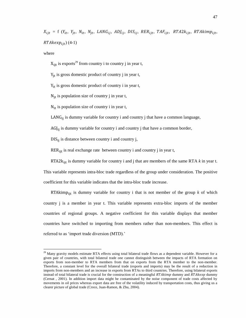
47

= f ( , , , , , , , , , , ,

) (4-1)

where

is exports29

from country i to country j in year t,

is gross domestic product of country j in year t,

is gross domestic product of country i in year t,

is population size of country j in year t,

is population size of country i in year t,

is dummy variable for country i and country j that have a common language,

is dummy variable for country i and country j that have a common border,

is distance between country i and country j,

is real exchange rate between country i and country j in year t,

is dummy variable for country i and j that are members of the same RTA k in year t.

This variable represents intra-bloc trade regardless of the group under consideration. The positive

coefficient for this variable indicates that the intra-bloc trade increase.

is dummy variable for country i that is not member of the group k of which

country j is a member in year t. This variable represents extra-bloc imports of the member

countries of regional groups. A negative coefficient for this variable displays that member

countries have switched to importing from members rather than non-members. This effect is

referred to as ‗import trade diversion (MTD).‘

29

Many gravity models estimate RTA effects using total bilateral trade flows as a dependent variable. However for a

given pair of countries, with total bilateral trade one cannot distinguish between the impacts of RTA formation on

exports from non-member to RTA members from that on exports from the RTA member to the non-member.

Therefore, a constant level for the overall bilateral trade (exports and imports) may be the result of a reduction in

imports from non-members and an increase in exports from RTAs to third countries. Therefore, using bilateral exports

instead of total bilateral trade is crucial for the construction of a meaningful dummy and dummy

(Cernat , 2001). In addition import data might be contaminated by the noise component of trade costs affected by

movements in oil prices whereas export data are free of the volatility induced by transportation costs, thus giving us a

clearer picture of global trade (Croce, Juan-Ramon, & Zhu, 2004).

48

is a dummy variable for country i that is a member of the group k of which

country j is not a member in year t. This variable represents extra-bloc exports of the member

countries of regional groups. A negative coefficient for this variable indicates that the RTA has

resulted in the member countries preferring to export to members rather than non-members. This

effect is referred to as ‗export trade diversion (XTD).‘

RTA dummies equal one since the date of a country‘s entry into the RTA30

. These three RTA

variables will allow us to determine the trade creation and diversion effects imputable to the

different groups and to see if they constitute building blocks or stumbling blocks to economic

progress. Trotignon (2010) draws up a typology of trade creation and diversion and systematizes

the summation of the three coefficients to all of the groups under examination as follows (Table

4-2 and Table 4-3):

Table 4-2: Typology of Trade Creation and Diversion

Designation Effect of Regional Grouping

Intra-bloc trade creation (ITC) Stimulating effect on trade between partners

Export trade creation (XTC) Stimulating effect on exports to the rest of the world

Import trade creation (MTC) Stimulating effect on imports from the rest of the world

Import trade diversion (MTD) Imports from the rest of the world are replaced by intra-bloc

trade

Export trade diversion (XTD) Exports to the rest of the world are replaced by intra-bloc trade

Source: Trotignon (2010), table 3, pp241

30

Since the number of members in some RTAs was not constant over the sample period and since some countries

acceded at a later stage, we had included in the three RTA dummies the countries according to the year when they

joined the agreement. According to Dee and Gali (2005), our RTA dummies are defined in dynamic form. In contrast,

antimonde form takes a nonzero value for all the years in the sample, irrespective of when the RTA was formed. Dee

and Gali (2005) compared between dynamic form and antimonde and they found that dynamic form play an important

role in their trade creation and trade diversion results.

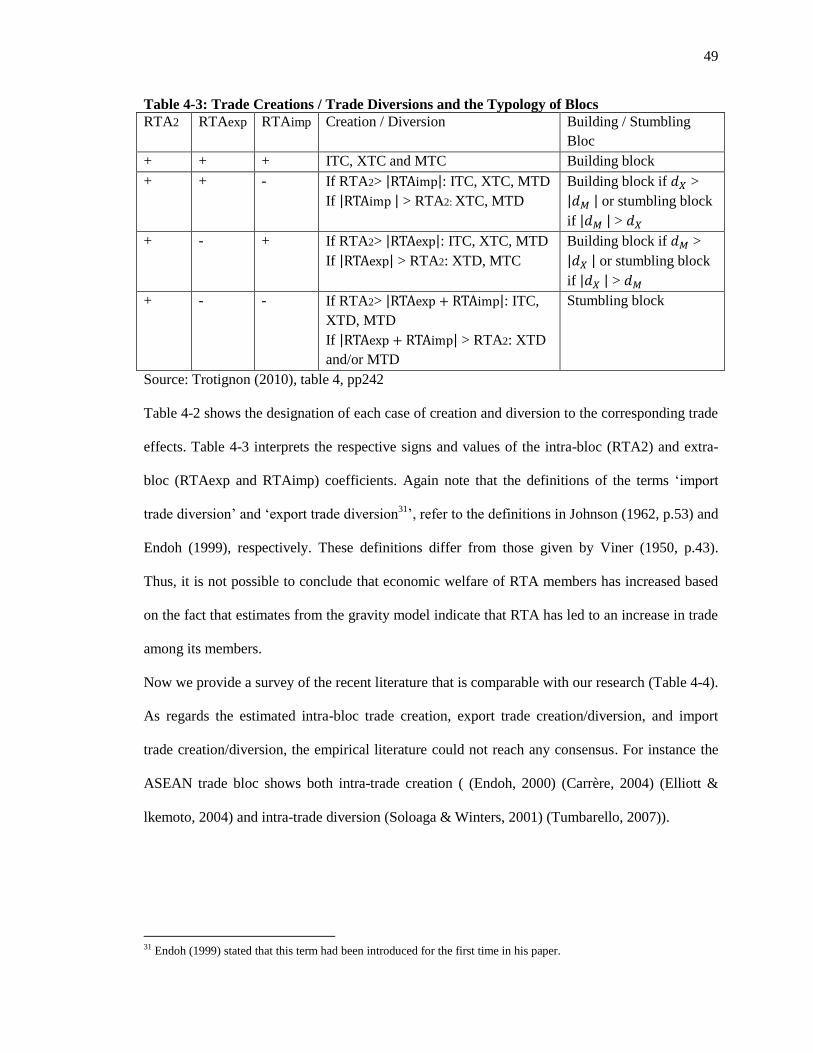
49

Table 4-3: Trade Creations / Trade Diversions and the Typology of Blocs

RTA2 RTAexp RTAimp Creation / Diversion Building / Stumbling

Bloc

+ + + ITC, XTC and MTC Building block

+ + - If RTA2> : ITC, XTC, MTD

If > RTA2: XTC, MTD

Building block if >

or stumbling block

if >

+ - + If RTA2> : ITC, XTC, MTD

If > RTA2: XTD, MTC

Building block if >

or stumbling block

if >

+ - - If RTA2> : ITC,

XTD, MTD

If > RTA2: XTD

and/or MTD

Stumbling block

Source: Trotignon (2010), table 4, pp242

Table 4-2 shows the designation of each case of creation and diversion to the corresponding trade

effects. Table 4-3 interprets the respective signs and values of the intra-bloc (RTA2) and extra-

bloc (RTAexp and RTAimp) coefficients. Again note that the definitions of the terms ‗import

trade diversion‘ and ‗export trade diversion31

‘, refer to the definitions in Johnson (1962, p.53) and

Endoh (1999), respectively. These definitions differ from those given by Viner (1950, p.43).

Thus, it is not possible to conclude that economic welfare of RTA members has increased based

on the fact that estimates from the gravity model indicate that RTA has led to an increase in trade

among its members.

Now we provide a survey of the recent literature that is comparable with our research (Table 4-4).

As regards the estimated intra-bloc trade creation, export trade creation/diversion, and import

trade creation/diversion, the empirical literature could not reach any consensus. For instance the

ASEAN trade bloc shows both intra-trade creation ( (Endoh, 2000) (Carrère, 2004) (Elliott &

lkemoto, 2004) and intra-trade diversion (Soloaga & Winters, 2001) (Tumbarello, 2007)).

31 Endoh (1999) stated that this term had been introduced for the first time in his paper.

50

Table 4-4: A survey of the recent literature using three regional dummy variables

Study Empirical

Approach

Period / #

of

countries

RTAs and Results

Endoh (1999) OLS 1960-1994 CMEA: RTA2=(+), RTAexp= (-), RTAimp= (-)

EEC: RTA2= (+), RTAexp= (+), RTAimp= (+)

LAFTA:RTA2= (-), RTAexp= (-), RTAimp = (-)

Endoh (2000) OLS 1995 ASEAN: RTA2 = (+), RTAexp= (+), RTAimp = (+)

APEC

EAEC RTA2 = (+), RTAexp= (+), RTAimp = (+)

Soloaga & Winters

(2001)

Tobit 1980-1996

/ 58

countries

ANDEAN: RTA2=(+), RTAexp=(-), RTAimp=(-)

ASEAN: RTA2 =(-), RTAexp=(+), RTAimp=(+)

CACM: RTA2 =(+), RTAexp=(-), RTAimp=(-)

EU: RTA2=(-), RTAexp=(+), RTAimp=(+)

EFTA: RTA2=(n), RTAexp=(+), RTAimp=(+)

GULFCOOP: RTA2=(+), RTAexp (-), RTAimp=(n)

LAIA: RTA2= (+), RTAexp=(-), RTAimp=(-)

MERCOSUR:RTA2=(+), RTAexp=(n), RTAimp=(-)

NAFTA: RTA2=(n), RTAexp=(n), RTAimp=(+)

Carrere (2004) Hausman-

Taylor

1962-1996 ANDEAN: RTA2=(+), RTAexp=(-), RTAimp (-)

MERCOSUR:RTA2=(+), RTAexp=(+), RTAimp=(-)

ASEAN: RTA2=(+), RTAexp=(+), RTAimp = (+)

CEMAC: RTA2=(+), RTAexp=(-), RTAimp=(-)

UEMOA: RTA2=(+), RTAexp=(-), RTAimp=(-)

ECOWAS: RTA2=(+), RTAexp=(-), RTAimp=(+)

SADC: RTA2=(+), RTAexp=(+), RTAimp=(-)

COMESA: RTA2=(n), RTAexp=(-), RTAimp=(n)

Croce, Juan-Ramon

and Zhu (2004)

Nonlinear 1978-2001

/ 64

countries

ANDEAN: RTA2=(n), RTAexp=(+), RTAimp=(n)

CACM : RTA2=(n), RTAexp (n), RTAimp=(-)

MERCOSUR:RTA2=(+), RTAexp=(-), RTAimp=(-)

NAFTA : RTA2= (+), RTAexp=(-), RTAimp=(-)

Elliott & lkemoto

(2004)

1982-1999 ASEAN RTA2 =(+), RTAexp=(+), RTAimp=(+)

EU: RTA2=(+), RTAexp=(+), RTAimp=(+)

NAFTA: RTA2=(+), RTAexp= (-), RTAimp = (-)

Kien & Hashimoto

(2005)

Hausman-

Taylor

1988-2002

/ 39

countries

AFTA: RTA2=(+), RTAexp=(+), RTAimp=(+)

EU: RTA2=(-), RTAexp=(n), RTAimp=(-)

MERCOSUR:RTA2=(+), RTAexp =(-),RTAimp=(+)

NAFTA: RTA2=(+), RTAexp=(-), RTAimp=(+)

Tumbarello (2007) 1984-2005

/ 182

countries

ASEAN: RTA2 =(-), RTAexp=(+), RTAimp=(+)

APEC: RTA2=(+), RTAexp=(+), RTAimp=(+)

CER: RTA2=(+), RTAexp=(+), RTAimp=(-)

EU-15: RTA2=(-), RTAexp=(+), RTAimp=(+)

EAEC: RTA2=(n), RTAexp=(+), RTAimp=(-)

MERCOSUR:RTA2=(+), RTAexp=(+), RTAimp=(-)

NAFTA: RTA2=(n), RTAexp=(-), RTAimp=(n)

SAPTA: RTA2=(n), RTAexp=(+), RTAimp=(+)

= intra trade, = export-extra trade, = import-extra trade, (+) = positive and statistically

significant, (-) = negative and statistically significant, (n) = not significant.

AFTA = ASEAN Free Trade Area, ANDEAN = ANDEAN Pact, ASEAN = the Association of

Southeast Asian Nation, APEC = the Asia Pacific Economic Cooperation, CACM = the Central

American Common Market, CEMAC = the Economic and Monetary Community of Central

Africa, CER = the Australia-New Zealand Closer Economic Relation, CMEA = the Council of

Mutual Economic Assistance, COMESA = the Common Market for Eastern and Southern Africa,

51

EAEC = East Asia Economic Caucus, EEC = the European Economic Community, ECOWAS =

the Economic Community of West African States, EFTA = the European Free Trade Association,

EU-15 = the European Union-comprising 15 members, GULFCOOP = Gulf Cooperation

Council, LAIA = the Latin American Integration Association, LAFTA = the Latin American Free

Trade Association, MERCOSUR = the Southern Common Market, NAFTA = the North

American Free Trade Agreement, SADC = the Southern African Development Community,

SAPTA= the Agreement on South Asian Association for Regional Cooperation Preferential

Trading Arrangement, UEMOA = the Economic and Monetary Union of West Africa,

The equation (4-1) comprising the three RTA variables will allow us to give an overall evaluation

of the process of regional integration vis-à-vis multilateral trade. We estimate two types of

specifications of equation (4-1). The first estimate includes three RTA dummy variables for 12

RTAs in a single regression in order to examine the effect of trade creation and the effect of trade

diversion in the interdependent context with other FTAs in the world. The second estimates each

RTA separately (12 separate regressions).

52

4.4 Data

4.4.1 Trade Data: The World Integrated Trade Solution (WITS) – the World Bank.

4.4.2 Data of Regional Integration: The Regional Trade Agreements Information System

(RTA-IS) – the World Trade Organization (WTO)

4.4.3 Data of Other Control Variables: The data on GDP, GDP per capita, and population

size are from World Economic Outlook Database – IMF. Language data are from Wikipedia

website (http://en .wikipedia.org/wiki). Data for tariffs is from United Nations TRANIS data,

World Integrated Trade Solution (WITS) Database. Exchange rate is obtained from IFS-IMF.

Note that ER is the exchange rate of the importer countries‘ currency measured by foreign

currency per unit of domestic currency. Hence, an increase (decrease) in ER indicates

appreciation (depreciation) of the domestic currency.

We report the summary statistics for all variables in table 4-5

53

Table 4-5: Summary Statistics

Definition Mean Std. Dev. Min Max

Exports in millions of $US. 201.7043 3,220.013 0 354,687

Importer Population (millions)

Importer GDP of $US (billions)

Exporter Population (millions)

Exporter GDP of $US (billions)

46.16.341

207.8676

36.35258

210.0203

156.8944

1,037.469

130.7271

909.7945

0.041

0.072

0.04

0.03

1,328.02

14,441

1,328.02

14,441

Importer‘s Tariff

Importer‘s Exchange Rate (Nati. per $US)

Distance

Contiguity

Language

14.5904

0.46887

8,084.103

0.0184

0.1608

11.35392

1.601

4,469.764

0.1344

0.3673

0

0

10.478

0

0

106.5

30.694

19,904.45

1

1

AFTA2

AFTA_imp

AFTA_exp

0.0029

0.0547

0.0457

0.0542

0.2274

0.2090

0

0

0

1

1

1

ADEAN2

ADEAN_imp

ADEAN_exp

0.0009

0.0370

0.0271

0.0308

0.1888

0.1624

0

0

0

1

1

1

CEMAC2

CEMAC_imp

CEMAC_exp

0.0004

0.0150

0.0176

0.0198

0.1216

0.1317

0

0

0

1

1

1

CIS2

CIS_imp

CIS_exp

0.0024

0.0359

0.0510

0.0486

0.1859

0.2200

0

0

0

1

1

1

EAC2

EAC_imp

EAC_exp

0.0005

0.0202

0.0155

0.0225

0.1406

0.1236

0

0

0

1

1

1

ECOWAS2

ECOWAS_imp

ECOWAS_exp

0.0068

0.0799

0.0621

0.0824

0.2712

0.2413

0

0

0

1

1

1

GCC2

GCC_imp

GCC_exp

0.0004

0.0141

0.0114

0.0211

0.1177

0.1059

0

0

0

1

1

1

MERCOSUR2

MERCOSUR_imp

MERCOSUR_exp

0.0005

0.0285

0.0205

0.0233

0.1664

0.1419

0

0

0

1

1

1

PAFTA2

PAFTA_imp

PAFTA_exp

0.00566

0.05813

0.05406

0.0750

0.2339

0.2261

0

0

0

1

1

1

SADC2

SADC_imp

SADC_exp

0.00212

0.03600

0.02507

0.0460

0.1863

0.1563

0

0

0

1

1

1

SAPTA2

SAPTA_imp

SAPTA_exp

0.00125

0.03800

0.02647

0.0353

0.1912

0.1605

0

0

0

1

1

1

WAEMU2

WAEMU_imp

WAEMU_exp

0.00128

0.03289

0.02115

0.0358

0.1783

0.1439

0

0

0

1

1

1

Number of OBS. 315,742

54

4.5 Results and Discussion

The results of the thirteen estimates are presented in Table 4-6. The first regression includes all

12 RTAs in a single pooled regression. The rest of the regression considers each RTA separately.

Since there appear to be missing observations of many control variables, this provides an

unbalanced panel. In the pooled estimation there are 315,742 observations containing 165

exporters and 158 importers over the period 1981-2008.

The model explains a high proportion –94 percent – of the total variation of world exports in the

single pooled regression and – between 79 to 96 percent in the each RTA separated regression.

Most of the basic variables of the gravity model – the level of GDP of exporter and importer,

importer‘s tariff, importer‘s exchange rate, distance, contiguity and language—have the expected

sign and are statistically significant. The coefficients of population for exporter and importer are

mixed. The coefficient on exporter GDP and importer GDP for example, is generally between 0.4

and 0.7, suggesting that trade increases as economic capacity grows. Distance variables and

common border variable always show the traditional negative sign and a positive sign,

respectively.

The PPML result suggests that during 1981-2008, RTA regimes had not brought the same

impacts in every regional trade grouping. Also PPML shows a different outcome for the pooled

regression and individual regressions. This study focuses on the result from pooled regression

because it examines the interrelationship among RTAs that allows comparing the trade impact of

these RTAs. Also the result for the pooled regression on average has a lower standard error

compared to the results for individual regressions.

4.5.1 AFTA (ASEAN Free Trade Area)

Two dummies; AFTA2 and AFTA_imp are positive and statistically significant. This means that

countries located within these regions give rise to intra-bloc trade creation and import trade

55

creation. Results show that the intra-regional trade for AFTA has increased to a higher level of

0.53. This means that AFTA members have trade with each other that is about 6932

percent higher

than without AFTA. This result shows that even though this study includes ASEAN new-comers

Cambodia, Lao P.D.R., Myanmar, and Vietnam, AFTA still fostered trade flows among

members. These new-comer members still have MFN tariff rates above those of other AFTA

members and they have a low trade share in the region.

A positive sign for the AFTA_imp variable suggests that AFTA members have not diverted their

imports from non-members to members. One plausible explanation for this is the fact that AFTA

members followed a long period of multilateral trade liberalization during the 1980s and 1990s.

In other words regional integration efforts proceeded in parallel with multilateral liberalization.

4.5.2 ANDEAN (Andean Community)

The RTA among the five countries (i.e., Bolivia, Columbia, Ecuador, Peru and Venezuela) seems

to have not significantly changed the trade pattern of their members during 1981-2008. This can

be seen from the insignificant coefficient of the ANDEAN2 and ANDEAN_exp. Only

ANDEAN_imp dummy is significant and negative. This implies import trade diversion.

4.5.3 CEMAC (Economic and Monetary Community of Central Africa)

Only CEMAC_imp dummy is significant in this RTA. This implies that CEMAC is associated

with import trade diversion. However, the CEMAC2-dummy is not significant in the pooled

regression but is negative and significant in the CEMAC individual regression. This implies that

under CEMAC there has been intra-trade diversion.

4.5.4 CIS (Commonwealth of Independent States)

The results suggest that CIS is associated with intra-bloc trade creation, export trade diversion

and import trade diversion. PPML shows that the intra-regional trade has increased about 100

percent. On the other hand, the results suggest that CIS members have preferred imports from

their members and exports to their members. On balance, the sum of the coefficients of three

32 [( -1)*100%]

56

dummy variables (1.008 + (-0.454) + (-0.416)) is equal to 0.138. This implies that CIS tends to

generate more trade among its members than any non-CIS random country pairs. In sum, the

results place CIS as a stumbling block to multilateral trade integration.

4.5.5 EAC (East African Community)

The results show that the EAC is related to intra-bloc trade creation, export trade diversion and

import trade diversion. The EAC agreement seems to have increased trade among its members

around 226 percent. This is shown by the positive and significant coefficient of the EAC2-

dummy. However EAC_import and EAC_export dummy are negative and significant. On

balance, the sum of the coefficients of three dummy variable (2.267 + (-0.421) + (-0.445)) is

equaled to 1.401. This indicates that EAC seems to have more intra-trade flows among its

members than non EAC random country pairs. In sum the results identify EAC as favorable to

trade regionalization.

4.5.6 ECOWAS (Economic Community of West Africa)

The results indicate that ECOWAS displays intra-bloc trade creation and import trade diversion.

If two countries are the members of ECOWAS, trade between them is 128 percent more than

without ECOWAS. Also ECOWAS appears to have 15.6 percent more imports among its

members than without ECOWAS. These results are similar to those of Carrere (2004) who

studied the period 1962-1996.

4.5.7 GCC (Gulf Cooperation Council)

GCC appears to have intra-bloc trade diversion and import trade creation. If two countries are

members of GCC, then trade flows between them average 112 percent less than two similar

countries. However the coefficient of GCC_imp dummy can be interpreted to mean that the GCC

agreement increases imports between its members and the rest of the world by approximately

16.5 percent. Our result is consistent with Al-Atrash and Yousef (2000). They presented evidence

that membership in GCC does not increase trade among member countries.

57

4.5.8 MERCOSUR (Southern Common Market)

The results indicate intra-bloc trade creation and import trade diversion. If two countries are

members of MERCOSUR, then trade flows between them average 68 percent higher than two

similar countries. On the other hand, the coefficient of MERCOSUR_imp dummy can be

interpreted to mean that the MERCOSUR decreases imports between its members and the rest of

the world by about 45 percent. Our result is consistent with Soloaga and Winters (2001) and

Croce, Juan-Ramon and Zhu (2004). They also found that trade integration and trade diversion

went hand in hand in MERCOSUR.

4.5.9 PAFTA (Pan-Arab Free Trade Area)

PAFTA appears to have intra-trade diversion and export trade creation. PPML indicates that if

two countries are members of PAFTA, then trade flows between them are 42 percent lower than

two similar countries.

4.5.10 SADC (Southern Africa Development Community)

SADC is the only RTA in this sample with three dummies (SADC2, SADC_exp and SADC_imp)

that are positive and statistically significant in the pooled regression. This means that countries

located within this region give rise to intra-bloc trade creation, import trade creation and export

trade creation. The result shows that SADC members have traded with each other about 208

percent higher than without the RTA.

In sum, PPML places SADC as a building block, favorable to both regional integration and

globalization.

4.5.11 SAPTA (Southern Asian Preferential Trade Agreement)

The result is associated with intra-bloc trade diversion and import trade diversion. SAPTA does

not seem to have fostered trade flows among members to any greater extent than trade with

nonmembers. PPML indicates that the intra-regional trade for SAPTA has decreased to a lower

level of 0.55, implying that SAPTA members have traded with each other about 42 percent less

than the level predicted in the benchmark context. Also SAPTA membership appears to have

58

been associated with import trade diversion. This can be seen from the negative coefficient of the

SAPTA_imp dummy. Our result is consistent with the World Bank (2004) report on South Asia‘s

trade. It argued that an RTA in South Asia would lead to substantial trade diversion rather than

trade creation and considers an RTA in the region as a stumbling bloc to multilateral trade

liberalization.

The World Bank report (2004) provided the reasons for the minimal impact during the earlier

years of the SAPTA as follow: (a) the extreme reluctance to make any meaningful concessions in

the earlier years. (b) The political problems between India and Pakistan exemplified by Pakistan‘s

short list of products that can be imported from India. This relationship has hamstrung SAPTA

and led all the South Asian countries to look for bilateral trade agreements with each other. (c)

India‘s import licensing system which continued to effectively ban imports of all consumer goods

from all destinations. The ban was lifted for the SAPTA countries only in 1998. It finally

disappeared for the rest of the world in April 2010. (d) The controls of India‘s agricultural

parastatals over imports and exports of major primary commodities.

4.5.12 WAEMU (West Africa Economic and Monetary Union)

In the case of the MAEMU PPML identified only intra-bloc trade diversion. PPML indicates that

the intra-regional trade for MAEMU has decreased to a lower level of 1.66, implying that SAPTA

members have traded with each other about 81 percent lower the level predicted in the benchmark

context.

59

Table 4-6: Intra and Extra-bloc Effects of Trade Agreement

All AFTA CAN CEMAC CIS EAC Exporter GDP 0.782***

(0.0506)

0.585***

(0.0577)

0.657***

(0.0850)

0.854***

(0.100)

0.076

(0.0732 )

0.460***

(0.0126)

Importer GDP 0.796**

(0.00967)

0.798***

(0.0715)

0.971***

(0.0822)

0.938***

(0.101)

0.337***

(0.0758 )

0.449***

(0.0201)

Exporter Pop. -0.0118***

(0.0437)

-0.147

(0.0854)

2.330***

(0.3331)

3.123***

(0.780)

0.781

(0.442) 1.133***

(0.0276)

Importer Pop. 0.0376**

(0.0116)

-0.230***

(0.0516)

-0.0689

(0.1043)

0.327

(0.266)

0.219**

(0.0736)

0.276

(0.0697)

Importer Tariff -0.0847***

(0.0177)

-0.235***

(0.0455)

-0.180**

(0.0684)

-0.0245

(0.147)

-0.141**

(0.0476)

0.0407

(0.0151)

Exchange Rate 0.00929

(0.00490)

-0.0895*

(0.0379)

-0.00431

(0.0091)

-0.0464

(0.0248)

0.0314

(0.0333)

-0.0611***

(0.00361)

Distance -0.644***

(0.0115)

-0.711***

(0.0292)

-1.717***

(0.0910)

0.257

(0.202)

-0.791***

(0.0559) -2.883***

(0.0352)

Contiguity 0.855***

(0.0318)

-0.0159

(0.0512)

0.120

(0.1195)

4.213***

(0.330)

0.255***

(0.0670)

-0.196

(0.0267)

Language 0.561***

(0.0220)

0.133***

(0.0358)

0.542*

(0.2734)

-0.280**

(0.108)

0.819***

(0.0979)

0.0269

(0.0106)

AFTA2 0.529***

(0.0793)

0.733***

(0.166)

AFTA_exp 0.0214

(0.0647)

0.591***

(0.153)

AFTA_imp 0.758***

(0.0352)

0.389*

(0.157)

ADEAN2 0.363

(0.209)

0.567*

(0.2679)

ADEAN_exp 0.0211

(0.204)

0.295*

(0.2679)

ADEAN_imp -0.497***

(0.0271)

0.264

(0.1357)

CEMAC2 -0.608

(0.355)

-2.116***

(0.382)

CEMAC_exp 0.279

(0.174)

-1.245***

(0.248)

CEMAC_imp -0.533***

(0.0811)

-0.885***

(0.183)

CIS2 1.008***

(0.172)

2.258***

(0.438)

CIS_exp -0.454**

(0.158)

1.219***

(0.224)

CIS_imp -0.416***

(0.0546)

1.288***

(0.227)

EAC2 2.267***

(0.154)

0.508*

(0.0331)

EAC_exp

-0.421**

(0.135)

0.361*

(0.0307)

EAC_imp -0.445***

(0.0560)

0.420**

(0.0280)

Standard errors in parentheses *p<0.05 **p<0.01 ***p<0.001

60

Table 4-6: Intra and Extra-bloc Effects of Trade Agreement (Cont.2/3) All ECOWAS GCC MERCOSUR PAFTA SADC

Exporter GDP 0.632***

(0.0754)

0.599***

(0.898)

0.456***

(0.0545)

0.568***

(0.0692)

0.537***

(0.122)

Importer GDP 0.608***

(0.0417)

1.163***

(0.503)

0.932***

(0.029)

1.152***

(0.0303)

0.711***

(0.159)

Exporter Pop. 1.273***

(0.274)

0.302

(0.192)

0.631**

(0.222)

0.0718

(0.121)

0.653

(0.438)

Importer Pop. 0.291***

(0.0684)

-0.113*

(0.057)

-0.253***

(0.0371)

-0.399***

(0.0322)

-0.728

(0.419)

Importer Tariff 0.00987

(0.0860)

0.269***

(0.046)

0.163***

(0.0438)

0.139***

(0.0405)

0.125

(0.0693)

Exchange Rate -0.0573***

(0.0156)

-0.297***

(0.043)

-0.012

(0.0112)

-0.178***

(0.0243)

0.0152

(0.0125)

Distance -0.0922

(0.0592)

-1.338***

(0.066)

-0.470***

(0.0265)

-1.096***

(0.0295)

-0.481***

(0.122)

Contiguity 0.888***

(0.117)

-0.447***

(0.095)

0.453***

(0.0818)

-0.699***

(0.0775)

1.606***

(0.176)

Language 1.166***

(0.0495)

0.353***

(0.067)

0.107*

(0.0518)

0.344***

(0.0438)

0.307**

(0.114)

ECOWAS2 1.284***

(0.208)

1.713***

(0.206)

ECOWAS_exp 0.0989

(0.191)

0.618

(0.735)

ECOWAS_imp -0.156**

(0.0535)

0.172

(0.105)

GCC2 -1.120***

(0.132)

-0.823***

(0.160)

GCC_exp 0.0925

(0.0977)

0.203

(0.135)

GCC_imp 0.165**

(0.0558)

-0.352***

(0.101)

MERCOSUR2 0.685***

(0.0962)

0.961***

(0.107)

MERCOSUR_exp 0.0448

(0.0679)

0.294**

(0.0999)

MERCOSUR_imp -0.452***

(0.0583)

0.583***

(0.0935)

PAFTA2 -0.421***

(0.0937)

-0.271*

(0.122)

PAFTA_exp 0.258**

(0.0928)

0.548***

(0.108)

PAFTA_imp 0.0491

(0.0351)

0.0346

(0.0988)

SADC2 2.087***

(0.180)

0.413

(0.219)

SADC_exp 0.717***

(0.132)

0.601***

(0.172)

SADC_imp 0.130*

(0.0618)

-0.0122

(0.153)

Standard errors in parentheses *p<0.05 **p<0.01 ***p<0.001

Table 4-6: Intra and Extra-bloc Effects of Trade Agreement (Cont.3/3)

All AFTA CAN CEMAC CIS EAC ECOWAS GCC MERCOSU

R

PAFTA SADC SAPTA WAEMU

Exporter GDP 0.774***

(0.0592)

0.762***

(0.161)

Importer GDP 0.824***

(0.121)

0.565***

(0.0676)

Exporter Pop. -0.203*

(0.0947)

1.043**

(0.357)

Importer Pop. 0.236

(0.186)

-0.114

(0.0664)

Importer Tariff -0.20***

(0.0603)

-0.13*

(0.0601)

Exchange Rate -0.115**

(0.0359)

-0.265***

(0.0422)

Distance -1.067***

(0.0306)

-0.0907

(0.0705)

Contiguity -0.322***

(0.0838)

0.914***

(0.135)

Language -0.479***

(0.0661)

0.599***

(0.107)

SAPTA2 -0.555**

(0.174)

-0.270**

(0.0892)

SAPTA_exp 0.0866

(0.0796)

0.396***

(0.0739)

SAPTA_imp -0.601***

(0.0435)

-0.0851

(0.0549)

WAEMU2 -1.668***

(0.162)

1.883***

(0.226)

WAEMU_exp -0.0839

(0.114)

0.779***

(0.187)

WAEMU_imp -0.0893

(0.0717)

1.239***

(0.165)

Constant 2.226***

(0.233)

4.455***

(0.704)

-0.246

(1.688)

-24.30***

(4.610)

0.743

(2.191)

15.26***

(0.478)

-10.28***

(1.470)

4.782***

(0.961)

-2.241

(1.230)

5.993***

(0.629)

-3.184

(3.167)

4.955***

()

-10.23***

(1.930)

All regressions include exporter fixed effect, importer fixed effect and time fixed.

N

Pseudo R-sq

315,742

0.941

36,243

0.960

23,816

0.949

18,853

0.877

30,068

0.953

24,261

0.877

59,732

0.888

26,584

0.923

18,306

0.963

68,897

0.880

50,106

0.882

63,131

0.936

35,925

0.798

Standard errors in parentheses *p<0.05 **p<0.01 ***p<0.001

61

62

4.6 Conclusion

Using a modified gravity equation, this chapter investigates the effects of RTAs on world and

regional trade patterns, concentrating on data for the 12 RTAs covering 1981-2008. The effects of

RTAs are captured by dummies that reflect intra-bloc trade and import extra-bloc trade and export

extra-bloc trade separately. Our first main finding is that not all of the RTAs succeed in giving rise

to intra-bloc trade creation. Some RTAs namely SAPTA, GCC, PAFTA, and WAEMU are found

to have negative intra-bloc effects. Our second finding is that of these 12 RTAs in the sample, 7

show import trade diversion while most of the export extra-bloc trade dummies are not statistically

significant. The third finding is that three of five African RTAs in the sample have generated intra-

bloc trade. Next, our finding is that the result for pooled regression and the result for individual

regressions are different. Finally our result confirms that the basic variables of the gravity model

show expected sign with high statistical significance (Table 4-7).

Table 4-7: Summary of regression results

Region RTA Type Regression Results

South East Asia AFTA FTA RTA2= (+), RTAexp= (n), RTAimp= (+)

South-Asia SAPTA PTA RTA2= (-), RTAexp= (n), RTAimp= (-)

Western Hemisphere ANDEAN CU RTA2= (n), RTAexp= (n), RTAimp= (-)

Western Hemisphere MERCOSUR CU &

EIA

RTA2= (+), RTAexp= (n), RTAimp= (-)

Europe and Central Asian CIS FTA RTA2= (+), RTAexp= (-), RTAimp= (-)

Middle East GCC CU RTA2= (-), RTAexp= (n), RTAimp= (+)

Middle East & North Africa PAFTA FTA RTA2= (-), RTAexp= (+), RTAimp= (n)

Sub-Saharan African CEMAC CU RTA2= (n), RTAexp= (n), RTAimp= (-)

Sub-Saharan African EAC CU RTA2= (+), RTAexp= (-), RTAimp= (-)

Sub-Saharan African ECOWAS CU RTA2= (+), RTAexp= (n), RTAimp= (-)

Sub-Saharan African SADC FTA RTA2= (+), RTAexp= (+), RTAimp= (+)

Sub-Saharan African WAEMU CU RTA2= (-), RTAexp= (n), RTAimp= (n)

Source: Authors‘ results

63

4.7 Appendix

Table A4-1: 12 Developing RTAs

AFTA

(ASEAN Free Trade

Agreement)

ANDEAN

(Andean Community )

CEMAC

(Economic and Monetary

Community of Central Africa)

Brunei Draussalam (1992)

Indonesia (1992)

Malaysia (1992)

Philippines (1992)

Singapore (1992)

Thailand (1992)

Vietnam (1995)

Laos (1997)

Myanmar (1997)

Cambodia (1999)

Bolivia (1988)

Columbia (1988)

Ecuador (1988)

Peru (1988)

Venezuela (1988)

Cameroon (1999)

Central of African Rep. (1999)

Chad (1999)

Congo, Republic of (1999)

Equatorial Guinea (1999)

Gabon (1999)

CIS

(Commonwealth of

Independent States)

EAC

(East African Community)

ECOWAS

(Economic Community of

West Africa)

Armenia (1995)

Azerbaijan (1995)

Belarus (1995)

Georgia (1995)

Kazakhstan (1995)

Kyrgyz Republic (1995)

Moldova (1995)

Russia (1995)

Tajikistan (1995)

Ukraine (1995)

Uzbekistan (1995)

Burundi (2000)

Kenya (2000)

Rwanda (2000)

Tanzania (2000)

Uganda (2000)

Benin (1993)

Burkina Faso (1993)

Cape Verde (1993)

Côte d'Ivoire (1993)

Gambia (1993)

Ghana (1993)

Guinea (1993)

Guinea-Bissau (1993)

Liberia (1993)

Mali (1993)

Niger (1993)

Nigeria (1993)

Senegal (1993)

Sierra Leone (1993)

Togo (1993)

Source: World Trade Organization

64

Table A4-1: 12 Developing RTAs (Cont.)

GCC

(Gulf Cooperation Council)

MERCOSUR

(Southern Common Market)

PAFTA

(Pan-Arab Free Trade Area)

Bahrain (2003)

Kuwait (2003)

Oman (2003)

Qatar (2003)

Saudi Arabia (2003)

United Arab Emirates (2003)

Argentina (1991) (Dummy

1992)

Brazil (1991)

Paraguay (1991)

Uruguay (1991)

Algeria (1998)

Bahrain (1998)

Egypt (1998)

Iraq (1998)

Jordan (1998)

Kuwait (1998)

Lebanon (1998)

Libya (1998)

Morocco (1998)

Oman (1998)

Qatar (1998)

Saudi Arabia ( 1998)

Syrian Arab Republic (1998)

Tunisia (1998)

United Arab Emirates (1998)

SADC

(Southern Africa Development

Community)

SAPTA

(Southern Asian Preferential

Trade Agreement)

WAEMU

(West Africa Economic and

Monetary Union)

Angola (2000) (Dummy 2001)

Botswana (2000)

Congo, Dem.Rep.of (2000)

Lesotho (2000)

Madagascar (2004)

Malawi (2000)

Mauritius (2000)

Mozambique (2000)

Seychelles (2001-2004, 2008)

South Africa (2000)

Swaziland (2000)

Tanzania (2000)

Zambia (2000)

Zimbabwe (2000)

Bangladesh (1995) (Dummy 1996)

Bhutan (1995)

India (1995)

Maldives (1995)

Nepal (1995)

Pakistan (1995)

Sri Lanka (1995)

Benin (2000)

Burkina Faso (2000)

Côte d'Ivoire (2000)

Guinea – Bissau (2000)

Mali (2000)

Niger (2000)

Senegal (2000)

Togo (2000)

Source: World Trade Organization

65

Chapter 5

Institutional Determinants of Foreign Direct Investment in ASEAN

5.1 Introduction

Foreign direct investment (FDI) inflows have grown faster than world income since the 1960s and

have risen much faster than world trade since the mid 1970s. Over the last couple of decades

worldwide FDI flows have increased by a factor of almost 10 while trade flows around the world

only doubled during a similar period. World FDI inflows have about tripled from $341 billion in

1995 to $973 billion in 2005 and world FDI inflows peaked at $1.38 trillion in 2000. These flows

have been concentrated in the developed countries which have accounted for more than 60 percent

of global FDI inflows, with the exception of 2004 when their share was 56 percent (Table 5-1).

Among the developing countries, ASEAN33

has been an important recipient of FDI. As a

percentage of World FDI, ASEAN in-flows jump from 1.7 percent in 2000 to 4.1 percent in 2005

but these flows have dropped from their highs in 1995 when ASEAN accounted for about 8.3

percent of world inflows34

. ASEAN is also one of the few developing-country areas that reports

bilateral FDI flows that constitute the dependent variable in this study.

33 The Association of Southeast Asian Nations (ASEAN) was founded in 1967. The five original members in 1976 –

Indonesia, Malaysia, the Philippines, Singapore, and Thailand – welcomed Brunei in 1984, Vietnam in 1995, Laos and

Myanmar in 1997, and Cambodia in 1999. ASEAN started implementing intra-regional economic cooperation in 1976.

In terms of an ASEAN economic integration, there are three pillars namely the ASEAN Free Trade Area (AFTA), the

ASEAN Investment Area (AIA) and the ASEAN Framework Agreements on Services (AFAS). ASEAN are widely

different from each other: ranging from land-locked, poor, rural Laos to the developed island city-state of Singapore. In

2009, the aggregate population was about 591 million growing at 1.2 percent annually. GDP for the region in 2009 was

$1,499 billion, so per capita GDP was $2,533. But that masked extreme variation from about $419 in Myanmar to

$36,631.2 in Singapore. (ASEAN Secretariat website, http://www.aseansec.org/19226.htm, accessed on January 01,

2011)

34 One possible explanation is this downward trend might be related to the Asian crisis. This crisis began in Thailand

with its currency crisis in 1997, which immediately had a great impact on other ASEAN countries. ASEAN countries

faced serious problems including negative economic growth, demand decline and stagnant FDI. However this downward

trend did not only affected ASEAN but also other region such as Africa, Central America, China and South Asia (Table

5-1).

66

Table 5-1: Percentage of world FDI inflows in developing countries by region (%)

Region 1995 1998 2000 2002 2004 2005

World (US$) 341,189 705,330 1,381,675 629,675 734,892 973,329

Total Developed Countries 64.8% 71.8% 80.9% 70.3% 56.4% 63.0%

Total Developing Countries 34.0% 27.6% 18.9% 28.9% 40.7% 32.3%

Africa35

1.7% 1.4% 0.7% 2.5% 3.0% 3.9%

South America36

5.5% 7.5% 4.2% 4.5% 5.1% 4.6%

Central America37

(8) 3.0% 2.3% 1.5% 4.1% 3.7% 2.6%

Caribbean38

(23) 0.2% 2.3% 1.5% 0.8% 4.2% 0.7%

China 10.6% 6.4% 2.9% 8.4% 8.3% 7.4%

Hong Kong + Korea

+Taiwan

2.7% 2.8% 5.5% 2.3% 6.1% 4.3%

South Asia39

(9) 0.8% 0.6% 0.4% 1.7% 1.4% 1.5%

ASEAN40

(10) 8.3% 3.2% 1.7% 2.7% 4.8% 4.1%

South-East Europe & the

Common wealth of Independent

States41

(20)

1.2% 1.1% 0.5% 1.8% 4.1% 3.2%

Source: UNCTAD (http://www.unctad.org/Templates/Page.asp?intItemID=3277&lang=1)

Note: Number in parenthesis is number of countries in each region

For ASEAN member countries, FDI remains one of the important keys to development. ASEAN

sought the deepening of intra-ASEAN economic cooperation and integration to attract FDI. Signed

in 1998, the ASEAN Investment Area (AIA) is a means of facilitating free flows of direct

investment, technology and skilled labor. The AIA opened up to ASEAN investors in 2010 and is

to be extended to all world investors by 2020. More recently, the AIA has been deepened through

the ASEAN Comprehensive Investment Agreement (ACIA), which was implemented in 2007.

35 Africa (56) : Algeria, Egypt, Libyan Arab Jamahiriya, Morocco, Sudan, Tunisia, Benin, Burkina Faso, Cape Verde,

Côte d' Ivoire, Gambia, Ghana, Guinea, Guinea-Bissau, Liberia, Mali, Mauritania, Niger, Saint Helena, Senegal, Sierra

Leone, Togo, Burundi, Cameroon, Central African Rep., Chad, Congo, Congo (Democratic Rep. of), Equatorial Guinea,

Gabon, Rwanda, São Tomé and Principe, Comoros, Djibouti, Eritrea, Ethiopia, Kenya, Madagascar, Mauritius, Mayotte,

Reunion, Seychelles, Somalia, Uganda, United Rep. of Tanzania, Angola, Botswana, Lesotho, Malawi, Mozambique,

Namibia, South Africa, Swaziland, Zambia, Zimbabwe. 36 South America (14): Argentina, Bolivia, Brazil, Chile, Colombia, Ecuador, Falkland Islands (Malvinas), French

Guiana, Guyana, Paraguay, Peru, Suriname, Uruguay, Venezuela. 37 Central America (8): Belize, Costa Rica, El Salvador, Guatemala, Honduras, Mexico, Nicaragua, Panama. 38 Caribbean (23): Anguilla, Antigua & Barbuda, Aruba, Bahamas, Barbados, British Virgin Island, Cayman Islands,

Cuba, Dominica, Dominica Rep., Grenada, Haiti, Jamaica, Martinique, Montserrat, Netherlands Antilles, Puerto Rico,

St. Kitts & Nevis, St. Lucia, St. Vincent & the Grenadines, Trinidad & Tobago, Turks & Caicos Islands. 39 South Asia (9): Afghanistan, Bangladesh, Bhutan, India, Iran, Maldives, Nepal, Pakistan, Sri Lanka. 40 ASEAN (10): Brunei Darussalam, Cambodia, Indonesia, Lao, Malaysia, Myanmar, Philippines, Singapore, Thailand,

Timor-Leste, Vietnam. 41 South-East Europe & the Common wealth of Independent States: Albania, Bosnia-Herzegovina., Croatia, Macedonia

Yugoslavia, Serbia & Montenegro, Armenia, Azerbaijan, Belarus, Georgia, Kazakhstan, Moldova, Russian Fed.,

Tajikistan, Turkmenistan, Turkmenistan, Ukraine, Uzbekistan.

67

This agreement covers further steps towards liberalization, protection, facilitation and promotion

of investments. Furthermore, it shortens the deadline to from 2020 to 2015 to achieve a free and

open investment environment. The objective of ACIA is to boost FDI inflows as a means to foster

economic growth through production and employment increases as well as spillover effects

(Uttama & Peridy, 2009).

Recently the literature has focused on the effects of institutions on FDI. There are several reasons

why the quality of institutions may matter for attracting FDI. One is rooted in the results of the

productivity and growth literature. Recent empirical evidence tends to confirm that cross-country

differences in growth and productivity are related to differences in institutions (Talbott & Roll,

2001). Good institutions may attract foreign investors. Another reason is based on studies by

North. According to North (1987), the fundamental causes of economic growth are the institutions

that lower transaction cost. Thus, poor institutions can bring additional transaction costs to FDI. A

third reason is high sunk costs. The high sunk costs associated with investing offshore, along with

weak enforcement of regulations and ineffective legal systems, has progressively forced

multinational firms to be increasingly selective as to where they will invest (Mishra & Daly,

2007).

Given the importance of foreign investment for ASEAN economies and given the importance of

institutions for attracting FDI, it is worthwhile studying the links between institutions and FDI.

This chapter contributes to the existing literature in several ways. First, we examine the role of

institutions in ASEAN over the period 1995 – 2005 by estimating a gravity equation for bilateral

FDI flows. Second I follow Santo Sila and Tenreyro (2006) and use a Poisson model pseudo –

maximum – likelihood (PPML) estimation technique. This estimation technique is robust to

different patterns of heteroskedasticity and provides a natural way to deal with zeros in the data.

Third the model incorporates more detail on institutions by using a new database constructed by

the French Ministry of Finance network in 51 foreign countries including ASEAN-6.

68

The remainder of the paper is organized as follows. A brief review of the literature is presented in

section 5.2. Section 5.3 presents the specification of the gravity model for FDI. Section 5.4

describes the data. Section 5.5 discusses the econometric specification for the gravity model

generated by the occurrence of zero FDI flows. Section 6 presents the empirical results and section

7 concludes.

5.2 Review of Literature

Several recent studies have focused on the role of institutions in determining the location of FDI in

this decade. Benassy-Quere et al. (2007) use data on bilateral FDI stocks from OECD countries

and find that bureaucracy, low corruption, information, banking sector and legal institutions have a

significant positive effect on FDI. They use the Institutional Profile database and the Fraser

database on institutional variables. Mishra and Daly (2007) study the effect of the quality of

institutions in the OECD and Asian host countries on outward FDI stocks of the OECD countries

using the International Country Risk Guide database (ICRG). They find that legal systems, popular

observance of law, strength and quality of bureaucracy and government stability in the host

countries have an overall positive and significant effect on source countries‘ outward FDI stocks.

Naude and Krugell (2007) use the World Bank database World Governance Indicators (

(Kaufman, Kraay, & Zoido-Lobaton, 1999)) to study institutional effects on FDI in Africa. They

find that political stability, accountability, regulatory burden and rule of law matter for FDI.

Asiedu (2006) using the data from ICRG finds that good infrastructure promotes FDI in Africa. In

contrast, corruption and political instability have the opposite effect. Aizenman and Mark M.

Spiegel (2006) find that the share of FDI to gross fixed investment as well as the ratio of FDI to

private domestic investment is negatively and significantly correlated with the level of corruption

and FDI is more sensitive than domestic investment to the level of institutional quality. Globerman

and Shapiro (2003) find that countries that fail to achieve a minimum threshold of effective

governance are unlikely to receive any US FDI. They also find that given that a country is a

69

recipient of US FDI, governance infrastructure as well as the nature of the legal system is an

important determinant of the amount received. Globerman and Shapiro (2002) use institutional

data from the World Bank, UNDP and Environmental sustainability Index. Their results indicate

that governance infrastructure is an important determinant of both FDI inflows and outflows. Stein

and Daude (2002) use ICRG data find that inward FDI to be significantly influenced by political

instability and violence, government effectiveness, regulatory burden, rule of law and graft.

All in all, recent evidence surveyed in Table 5-2 confirms a straightforward picture. The quality of

institutions is an important determinant of FDI activity. This suggests that institutional changes in

ASEAN may have influenced the variance of FDI in ASEAN42

. The next section therefore applies

a gravity model of FDI with institutional variables and refined empirical techniques to check

whether a robust result can be obtained for ASEAN.

42

It is surprising that there is a lack of research on the institutional determinants of FDI in ASEAN. A search of the

EconLit database typing ‗foreign direct investment‘ and ‗ASEAN‘ and ‗institutions‘ as keywords yielded zero journal

articles the institutional determinants of FDI to ASEAN.

70

Table 5-2: Selected recent studies concerning institutions and FDI Study Empirical

Approach

Sample Data for

Institution43

Other Control Variables44 Conclusion

Desbordes and

Vicard (2009)

Poisson , OLS OECD

1991-2000

ICRG, KEDS GDPH, GDPS, GDPCAPH,

GDPCAPS, DIST, LANG, BIT

Positive & sig.

link b/w instit.

& FDI

Benassy-

Quere et al.

(2007)

Three step

precedure

OECD

1985-2000

IP and Fraser GDPH, GDPS, GDPCAPH,

DIST, Contiguity, LANG

Positive & sig.

link b/w instit.

& FDI

Mishra and

Daly (2007)

2SLS OECD

1991-2001

ICRG SGDP, DIST, TRADE,

ADIFSKILL

Positive & sig.

link b/w instit.

& FDI

Naude and

Krugell (2007)

GMM Africa 1970-

1990

KKZL Lag of (FDI/GDP) Negative &

Positive & Sig.

Asiedu (2006) FE Africa 22

countries

1984-2000

ICRG NATEXP, GDP, INFLT, LIT,

INFR, Political Risk

Positive & sig.

link b/w instit.

& FDI

Aizenman and

Mark M.

Spiegel (2006)

Weighted least

squares

A cross

country

1990-99

Business

International‘s

index

GDP, DISTUS, DISTGERM,

SKILL, SKILLGDP, INVC,

PROT

Positive & sig.

link b/w instit.

& FDI

Globerman

and Shapiro

(2003)

A two-stage

estimation: 1st

stage is probit

and 2nd stage

is OLS

A cross

country

1995-1997

KKZL RGDP, HDI, FIXUS, DEXR,

PROX

Positive & sig.

link b/w instit.

& FDI

Globerman

and Shapiro

(2002)

OLS A cross

country

1995-97,

FDI in. &

FDI out.

KKZL, HDI,

ESI

Lag GDP Positive & sig.

link b/w instit.

& FDI

Stein and

Daude (2002)

OLS, 2SLS &

Robustness

(Poisson,

Tobit)

A cross

country

2002

Outward

FDI stock

KKZL,

ICRG, WBEC

SGDP, SQDIFGDP,

ADIFGDP*ADIFSKILL,

ADIFSKILL, DIST, TARIFF,

TARIFF*SQDIFSKILL

Positive & sig.

link b/w instit.

& FDI

Hausmann and

Fernandez

(2000)

OLS A cross

country

1996-98

KKLP, La

Porta

GDPCAP, GDP, TRADE2 Positive & sig.

link b/w instit.

& FDI

43

Business International‘s Index from the Tanzi and Davoodi (1997) (http://www.transparency.org/), ESI =

Environment Sustainability Index by the World Economic Forum in conjunction w/ Columbia and Yale Universities,

Fraser = the Fraser Institute database, HDI = UN Human Development Index by the United Nation, ICRG =

International Country Risk Guide, IP =the Institutional Profiles database, KEDS = the Kansas Events Data System by

Gary King (http://gking.harvard.edu.), KKZL = Kaufmann et al. (1999a, b), La Porta = the La Porta et al. (1997, 1998a,

1998b), WBEC = Business Environment Survey from the World Bank. 44

ADIFGDP = the absolute difference b/w the host country and the source country GDPs, ADIFSKILL = the absolute

difference b/w the countries‘ endowments of skilled labor, DEXR = Exchange rate change, DIST = the distance b/w the

capital of the host country and the source country, DISTUS and DISTGER = the log of distance from the US and

Germany, respectively, FIXUS =countries with fixed exchange rate dummy,GDPH and GDPS = the log of the host

country GDP and the source country GDP, respectively, GDPCAPH and GDPCAPS = the log of the host country and

the source country GDP per cap, INVC = investment costs and protectionism from Markusen and Maskus (2002) based

on the World Competitiveness Report of the World Economic Forum, INFLT = Inflation, INFR = the # of telephone

main lines per 1,000, LIT= the % of adults who are literate, NATEXP = the share of minerals & oil in total exports,

PROX = a dummy that equals 1 if the country is contiguous with the US, Political Risk = Coups Assassinations and

Revolutions from the Cross-national Time Series Data Archive, RGDP = real GDP, SGDP = the sum of the logs of the

host country and the source country GDPs ($), SKILL = the ratio of skilled to unskilled labor in country i, SKILLGDP =

the ratio of skilled labor w/ the size of the local economy, SQDIFGDP = the squared difference in the GDPs of the host

and the source country, SQDIFSKILL = the squared difference b/w the countries‘ endowments of skilled labor,

TRADEa = the ratio of trade to GDP, TRADEb = the ratio of export to GDP, TARIFF = average tariff

71

5.3 Gravity Model of FDI

The empirical specifications of this paper are based on Kleinert and Toubal‘s (2010) gravity model

of FDI and based on Blonigen (2005)‘s review of the empirical literature on FDI determinants. We

add institutional variable (INST) into their models. The next two equations are the gravity model

of FDI following Kleinert and Toubal‘s (2010) work. The further two equations are equation (5-1)

and (5-2) that include Blonigen (2005) four variables.

Equation (5-1) gives the standard gravity equation for FDI as derived from the horizontal

models45

.

= f( , , , ) (5-1)

where subscript i, j and t denotes home country, host country and time, respectively. Y indicates

GDP and D indicate distance between home and host country. The horizontal models predict the

coefficients of the home and host country GDP to be one. The distance coefficient β is predicted to

be negative. The regression model derived from the vertical model is given by

= f( , , , , + , ) (5-2)

where = (( ) / ( )), L denotes the factor price of low-skilled labor

and S indicates the factor price of high-skilled labor. The vertical model predicts the coefficient ϑ

of the sum of home and host countries GDP to be one, the coefficient ζ to be negative, and ξ to be

positive. Additionally the distance coefficient β is predicted to be negative while the coefficient

of the relative factor endowment RFE should be positive.

45

Shatz and Venables (2000) distinguished between two main reasons why foreign direct investors would like to locate

in a foreign country. The first one is to better serve the local market and is called ‗horizontal‘ or ‗market seeking‘

(market access motivation) since it implies a duplication of production plants. Here the main motivation is to economise

on tariffs, transport costs and to tap a new market. FDI to establish a horizontal MNE is a substitute for international

trade and is mainly driven by market size. The second reason is to have access to lower-cost inputs. This type of FDI is

called ‗vertical‘ or ‗production cost-minimizing‘ (resource access motivation) since there is fragmentation. The

motivation is to economise on production factors to maximize the profits on each part of the good production.

72

Blonigen (2005) reviews the empirical literature on FDI determinant and he concludes that

exchange rate effects, taxes, institutions, trade protection, and trade effects matter for the firm‘s

FDI decision. Thus, we include exchange rate (ER), trade openness (OP), average tariff (TARF),

corporate income tax (TAX) into the equation (1) and equation (2), respectively.

= f( , , , , , , , ) (5-3)

= f( , , , , + , , , , , ) (5-4)

Accordingly, we use equation (5-3) and (5-4) to study the influence of institutions of FDI in

ASEAN. Given the high degree of correlation among the institutional variables, we include them

in the regressions one at a time in order to avoid problems of multicollinearity. The details of

institutional variables are shown in the next section.

73

5.4 Data

5.4.1 FDI Data

We use bilateral FDI inflows into ASEAN countries from the Statistics of Foreign Direct

Investment in ASEAN, Eighth Edition, (2006) covering the period from 1995 to 2005. To our

knowledge, this is the only database that covers bilateral FDI inflows to all ASEAN countries and

one of the few such databases extant among developing-country groups. The dataset covers 39

source (home) countries46

and 9 host countries47

which include all ASEAN members. Since some

host countries namely Brunei Darussalam, Cambodia, and Lao PDR have not data on many control

variable, this study can cover only ASEAN6, namely; Indonesia, Malaysia, the Philippines,

Singapore, Thailand, and Vietnam. There also are the negative divestment figures (352

observations). We treat them as zero observations. Thus, forty-two percent of the bilateral

dependent-variable observations are zero FDI inflows.

5.4.2 Institutional Data

In order to assess the role of institutions as a determinant of the amount and the location of FDI,

we primarily use a database called Institutional Profiles that describes both formal and informal

institutions at a highly detailed level. The database was built by researchers from the French

Ministry for the Economy, Industry and Employment (MINEIE), and the French Development

Agency (AFD) and was constructed from a world survey conducted with MINEIE and AFD

agencies present in the countries covered in the database.

A total of 356 questions were asked concerning public institutions, good and services, capital

markets, and labor markets. In each case, a set of questions were asked covering nine institutional

46 Source (Home) countries are Japan, USA, Canada, Austria, Belgium, Denmark, Finland, France, Germany, Greece,

Ireland, Italy, Luxembourg, Netherlands, Portugal, Spain, Sweden, United Kingdom, China, India, Pakistan, Republic of

Korea, Hong Kong, Taiwan (China), Brunei Darussalam, Cambodia, Indonesia, Lao PDR, Malaysia, the Philippines,

Singapore, Thailand, Vietnam, Australia, New Zealand, Argentina, Brazil, Mexico, Panama. 47 Host countries are Brunei Darussalam, Cambodia, Indonesia, Lao PDR, Malaysia, the Philippines, Singapore,

Thailand, Vietnam

74

functions namely: (1) political institutions, (2) safety, law and order, (3) public governance, (4)

market freedom, (5) investment on future, (6) ability to reform, (7) security of transaction and

contracts, (8) regulation, and (9) openness and social cohesion. The responses to each question

ranked 0, 1, 2, 3 and 4. Higher values indicate better institutions (0 very bad to 4 very good)

(Meisel & Aoudia, 2007). Table 5-3 shows the structure of the institutional field.

We access the Institutional Profiles Database (IPD) from the Centre D‘ etudes Prospective Et D‘

information Internationals (CEPII). The IPD is based on a survey conducted in 2001 and in 2006.

The 2001 IPD covered 51 countries and 2006 IPD extended to 85 countries (including the 51

countries in the 2001 IPD). Both IPD included ASEAN countries. We use 2001 IPD for FDI over

the period 1995-2000 and use 2006 IPD for FDI over the period 2001-200548

.

48

http://www.cepii.fr/anglaisgraph/bdd/institutions.htm

75

Table 5-3: A summary of the database and its structure in 4 sectors and 9 themes

Institutional themes

in the columns

Institutional

environment

Markets

Institutional themes

in the row

-A- Public

institutions, Civil

society

-B- Good and

services

-C- Capital

market

-D- Labor

markets and

social relations

1. Political institutions Public rights and

liberties

Trade union

freedom and

pluralism

2. Safety, law and

order

Safety of persons

and goods

3. Public governance Transparency,

corruption control,

efficiency of

administration,

independence of

the justice system

Business start-ups

4. Markets‘ operating

freedom

Share of the

private sector,

privatization,

price distortions

introduced by the

government

Share of the

private sector,

freedom of

interest rates,

independence of

the central bank

Share of public-

sector,

employment,

flexibility of the

formal labor

market

5. Technological

environment,

Expectations

Innovations and

the authorities‘

strategic vision

Businesses‘

technological

environment

Venture-capital Vocational

training

6. Security of

transactions and

contracts

Security of

property rights

and contracts,

commercial

justice,

bankruptcy law

Information on

the quality of

goods, the

situation of firms,

intellectual

property

Guarantee

systems,

obligation to

provide

information

Respect for labor

laws

7. Regulations and

corporate

governance

Regulation of

competition

Regulation of

competition,

corporate

governance

Regulation of

competition,

prudential rules,

supervision

Social dialogue

8. Openness to the

outside world

Circulation of

persons and

information

Trade openness Financial

openness

Circulation of

workers

9. Social cohesion Social

equilibrium,

equality of

treatment, social

mobility,

solidarity

Micro-leading Market

segmentation and

social mobility

Source: http://www.cepii.fr/anglaisgraph/bdd/institutions.htm

76

The advantages of this database consist of the following. First, the respondents are relatively

homogenous since all of them are French civil servants working in each of the country surveyed

(Benassy-Quere, Coupet, & Mayer, 2007). Second, the IP database is focused from the start on the

issues of long-term growth and development49

(Meisel & Aoudia, 2007). Third, the IP database

covers a large number of institutional aspects50

. Here we work at the first level of aggregation, i.e.

on 96 institutional variables. Since institution variables are often correlated with one another, it is

generally not possible to include several institutions in the single equation. Thus here we introduce

each of the 96 institution variables in estimation where the institutional variable is limited to only

one variable – the institutional characteristic of the host country.

5.4.3 Data on other control variables

The nominal GDP and GDP per capita (GDPCAP) are in US dollars. OP is total trade as

percentage of GDP. Data on GDP, GDPCAP and OP have been taken from the World

Development Indicators database of the World Bank. Time-invariant bilateral characteristics

(distance, contiguity and common language) are obtained from the Centre D‘ etudes Prospective

Et D‘ information Internationals (CEPII). The labor (RFE) is given as the share of home country

skilled labor in total skilled labor of the two countries, , and the share of home‘s

unskilled labor, . These are obtained from the World Development Indicators data

base of the World Bank. Exchange rate (ER) is obtained from International Financial Statistics of

the International Monetary Fund. Average Applied Tariff Rates (TARF) is obtained from the

World Bank51

. Corporate income tax (TAX) is obtained from KPMG‘s Corporate Tax Rate

Survey. Summary statistics are shown in Table 5-4. Note that ER is the exchange rate of the host

49

Other databases have different focuses. For instance, the Freedom House provides an institutional database focusing

on the evaluation of freedom in the world. See: http://www.freedomhouse.org. 50

Meisel and Aoudia (2007) compared the IPD to the six governance indicators used by the World Bank Institute

(WBI), using two principal components analyses (PCAs). They shown that the IPD covers a much vaster institutional

field of governance described by the WBI‘s indicators. 51 Permanent URL for this page: http://go.worldbank.org/LGOXFTV550

77

countries currency measured by foreign currency per domestic currency. Hence, increase

(decrease) in ER indicates appreciation (depreciation) of domestic currency.

Table 5-4: Summary Statistics

Definition Mean Std. Dev. Min Max

FDI inflow (millions $) 97.4001 371.2228 0 7921.7

Home GDP ($)

Host GDP ($)

Distance

Sum of GDP

Relat. Factor Endow.

1.23e+11

2.46e+18

8039.443

2.46e+18

1.10995

5.15e+10

1.51e+19

5011.799

1.51e+19

.2363716

6.52e+10

1.28e+09

315.5433

6.65e+10

.3841963

2.86e+11

1.21e+20

19276.41

1.21e+20

1.628932

Exchange Rate ($)

Openness

Tariff

Cor.Tax

.192495

109.3162

7.950982

29.25455

.2390435

52.11392

5.037481

3.488309

.000098

52.26474

0

20

.7092199

220.4073

19.8

39

a100 |

a150

a101

a151

a102

2.534088

2.181818

2.279975

2.090909

2.073962

.4473202

.6944681

.7612833

.6450922

1.017186

1.831356

1

.7844934

1

1

3.31462

3

3.482011

3

4

a103

a104

a200

a201

a250

2.857187

1.808739

2.677994

3.30303

1.742424

1.113117

.754306

.764064

.7583328

.5855616

1

1

1.724172

2

1

4

3

4

4

3

a300

a301

a350

a302

a351

2.301153

2.670741

2.666667

1.97079

1.914955

.6404134

.7265597

.4714985

1.007908

.642332

1.486292

1

2

1

0

3.804364

4

3

4

2.55948

a303

a352

a304

a353

a354

2.035783

2.257576

1.905337

1.65839

2.515152

.9468231

.5855616

1.069132

.884989

.49987

1

1

1

0

2

4

3

4

3.416303

3

a305

a307

a355

a356

a510

2.632386

2.126225

2

1.603782

2.827094

.5699807

.6610501

.4264865

.7803479

.74874

1.98194

1

1

.5044457

1.287388

3.657241

2.987386

3

3.011151

4

a511

a512

a513

a515

a600

2.484349

2.969697

2.650331

3.136364

2.273547

.678694

.9371338

.7893345

.7957214

1.257895

1

1

1.321426

2

0

3.369358

4

4

4

4

a601

a602

a603

a604

a605

2.834367

3.056628

2.724789

3.106061

2.384438

.6694054

.6812405

.5778828

.6000957

.7761187

1.760475

2

2

2

1

4

4

3.724256

4

3.520639

78

Table 5-4: Summary Statistics (Cont.)

Definition Mean Std. Dev. Min Max

a606

a607

a650

a800

a803

a900

a901

2.414379

1.865376

2.484848

3.28475

2.041404

2.645441

2.937086

1.106463

.6051027

.49987

.4539458

.8179781

.6944467

.8457546

.5001568

1.321279

2

2.631551

.3238837

1.657739

1.635442

4

3.006459

3

4

3.676116

3.663048

4 a902

a903

a904

2.256295

3.395547

1.566359

.9002647

.2913632

.6925173

1

2.91706

.6156725

3.556741

4

3.074262

b300

b400

b403

b451

b452

2.485392

2.227273

2.814514

2.324815

2.325502

.7456693

.5979804

.7179933

.5404238

.5633388

1.26435

1

1.821388

1.247295

1.351357

3.650182

3

4

3.251163

3

b500

b600

b602

b603

b604

2.485392

2.571295

2.681818

1.789318

2.11881

.7456693

.7310437

.8378965

.9331637

.9702582

1.26435

1.40037 1

1 .869822

3.650182

4

4

4

4

b700

b701

b702

b704

b710

2.513475

2.712121

1.166667

2.84349

2.5

.7245253

.9174442

1.0674

.7403552

.857404

1

1

0

2

1

4

4

3

4

4

b800

c400

c402

c453

c500

3.330639

2.575758

2.536851

1.201027

2.333333

.6681107

.8716164

.6660507

.7769575

1.034956

1.536682

1

.9167659

0

1

4

4

3.189826

2.556332

4

c501

c502

c600

c601

c602

1.893939

2.110525

2.670279

2.969697

2.791219

1.338841

.7809544

.6751578

8069574

1.10792

0

.4433451

1 .

1

.4894912

4

3.601135

3.522806

4

4

c603

c700

c702

c703

c704

2.893939

3.090909

3.034074

2.783178

2.53363

.8728013

.8831338

.8716067

1.005175

.9110422

1

1

1

1

1

4

4

4

4

4

c750

c800

c850

c900

d100

2.523042

1.843268

2.541977

1.777043

1.920497

.8330718

.5777314

.9208475

1.042111

.8023954

1

.7804589

1

0

.9410718

3.683491

2.912283

4

3.546893

3.777451

d101

d401

d450

d500

d600

2.681818

3.415177

.3378381

2.132177

2.128788

1.316353

.4063758

.5510506

.9328717

.9018223

1

2.612047

0

1

1

4

4

1.513412

3.549703

4

d601

d602

d603

d700

d701

1.77248

2.419554

1.880171

3.333333

2.148489

.9172066

.5458017

.9179229

.7455046

.7510727

0

1.698813

0

2

.7702506

3.55462

3.395849

3

4

3.420785

79

Table 5-4: Summary Statistics (Cont.)

Definition Mean Std. Dev. Min Max

d800

d900

d901

d902

d903

d950

2.54147

2.648517

2.637021

3.046968

2.590909

.3973346

.5210922

.4501034

.7113352

.6995445

1.124708

.7317732

1.461837

1.671897

1.461863

1.629265

1

0

3.494708

3.280305

4

3.697942

4

2

5.5 Results

In order to avoid the problems of multicollinearity, we include institutional variables in the

regressions one at a time. Estimates which are institutional coefficients and their standard errors

are similar between specification (5-3) which derived from the horizontal FDI model and

specification (5-4) which derived from the vertical FDI model. The results are reported in table 5-5

for the total 34 best fits (out of 96 regressions). Note that all specifications include a full set of

time, home, and host country fixed effects. The robust standard errors have been computed. The

model explains a high proportion – approximately 70 percent – of the total variation of FDI inflow

to ASEAN. In most cases, the coefficient of the institutional variables is significant at the one

percent level and positive. Taking into account control variables in specification (5-3) and in

specification (5-4), distance, corporate income tax, and home country GDP have a significant and

expected sign. We present all detail of regression results.

In most of 34 best fits, the estimates have the predicted sign. This means that good institutions in

the host country have a positive impact on bilateral FDI in ASEAN. Variables namely political

rights and functioning of political institutions, quality of local authorities, transparency of public

action, lack of corruption, good government-citizen relations, effectiveness of public action,

security of traditional property rights, law on bankruptcies, the security of transactions, ,

intellectual property, arrangements for fall into this category. Furthermore the results highlights

the importance of share of public sector in GDP, the protection of intellectual property,

competition between businesses: competition regulation arrangements, liberalize the credit sector,

80

dissemination of technology, innovation, lender guarantees, banking and financial supervision, the

regulation of the financial system, reforms to make the formal labor market more flexible, labor

legislation and measures, and labor inspectorate for inward FDI. These results confirm that good

institutions promote inward FDI.

The quality of some institutions in the host country has a sizable impact on inward FDI. In table 4-

6, we present the institutional data for our 34 best fits. For instance, host countries that had

improvements in level of transparency of public action (A350) such as Indonesia and Thailand

from in 2001 with a variable equal to 2 to in 2006 with a variable equal to 3, they are estimated to

receive 38.1352

percent more FDI. On the other hand, host countries that had decline in level of

transparency of public action such as Malaysia and Philippines from a variable equal to 3 in 2001

to 2 in 2006, they are estimated to 27.6053

percent less FDI. For arrangements for the protection of

intellectual property (B604), comparing Vietnam with a lowest level (a variable equal to 1) to

Singapore with the highest level (a variable equal to 4), PPML leads to a 325 percent more FDI

received if Vietnam are able to improve their level to Singapore level.

In addition our results indicate that good institutions discourage FDI. The institutions that fall in

this category consist of public freedoms and the autonomy of the civil society, internal public

security, running of the customs administration, free movement of persons and information,

implementation of the privatization program, openness of the privatization program, dissemination

of technology, information on the structure of shareholdings in local firms, insurance companies,

competition within the banking system, openness to foreign capital and loans, and rigidity of the

formal labor market. However these results should not be interpreted to mean in order to attract

FDI, ASEAN countries should reduce qualities of those institutions. They are able to interpret that

there is no direct positive effect of those institutional variables on FDI.

52 38.13 percent = [exp(1*0.323)-1]*100% 53

-27.60 percent = [exp(-1*0.323)-1]*100%

81

Comparing our results to the other empirical studies, we find that there are only two studies that

indicate a negative relation between institutions in the host country and FDI inflow54

: Naude and

Krugell (2007) and Benassy-Quere, Coupet and Mayer (2007). The latter use the same source of

institutional variables as we do in this study. They found two cases having negative link between

institutions and FDI inflow and those two cases are not significance in our study. In our

regressions there are two cases having negative impact between institutions and inward FDI that

shown positive relation in Benassy-Quere, Coupet and Mayer (2007). In Naude and Krugell

(2007), they used KKZL data and found that political stability and accountability have a negative

impact. However, they have no addition explanation for these relations.

Finally in table 4-6 we summarize the results in framework of institutional themes. We found that

security of transactions and contracts have strong relation to increase FDI inflow in ASEAN

countries. In addition, public governance has a second rank of promoting FDI in ASEAN.

54

As shown in our table 5-2, most of the recent studies indicated positive link between institutions and inward FDI.

Table 5-5: Estimates of Equation (5-3) – Equation (5-4) with IP data

Code Institutions

Eq.(5-3) Eq.(5-4)

Coeff. se R-sq Coeff. se R-sq

1 A100 Political rights and functioning of political institutions 1.579*** (0.428) 0.739 1.582*** (0.433) 0.730

2 A101 Public freedoms and the autonomy of the civil society -1.311* (0.616) 0.726 -1.292* (0.622) 0.727

3 A103 Centralization - decentralization: devolution of local authorities 2.248*** (0.479) 0.732 2.334*** (0.481) 0.728

4 A200 Internal public security -0.890* (0.395) 0.727 -0.952* (0.392) 0.728

5 A350 Evolution of transparency of public action in the past 3 years 0.323* (0.141) 0.727 0.362* (0.142) 0.729

6 A302 (Lack of) Corruption / Corruption 1.135*** (0.328) 0.730 1.226*** (0.326) 0.731

7 A351 Evolution of petty and large-scale corruption in the past 3 years 0.574** (0.211) 0.727 0.594** (0.209) 0.729

8 A303 Government-citizen relations 0.302* (0.151) 0.727

9 A304 Effectiveness of public action: tax system 0.994** (0.361) 0.728 1.102** (0.363) 0.730

10 A305 Running of the customs administration -1.307*** (0.361) 0.730 -1.373*** (0.360) 0.731

11 A600 Security of traditional property rights 0.814*** (0.233) 0.730 0.844*** (0.232) 0.731

12 A606 Law on bankruptcies 0.544* (0.257) 0.726 0.541* (0.257) 0.727

13 A650 Evolution of the security of transactions in the past 3 years 0.536* (0.271) 0.726 0.584* (0.266) 0.727

14 A800 Free movement of persons, information, etc -0.773* (0.316) 0.728 -0.847** (0.317) 0.729

15 B400 Share of public sector in GDP 0.564* (0.262) 0.728

16 B451 Implementation of the privatization program -1.113*** (0.311) 0.729 -1.131*** (0.310) 0.730

17 B452 Openness of the privatization program -0.881* (0.412) 0.726 -0.880* (0.413) 0.727

18 B500 Technological environment, dissemination of technology -0.967* (0.450) 0.726 -0.975* (0.449) 0.727

82

Table 5-5: Estimates of Equation (5-3) – Equation (5-4) with IP data (Cont.)

Code Institutions

Eq.(5-3) Eq.(5-4)

Coeff. se R-sq Coeff. se R-sq

19 B603 Intellectual property 2.265*** (0.646) 0.729 2.351*** (0.642) 0.731

20 B604 Arrangements for the protection of intellectual property 0.483* (0.223) 0.728

21 B702 Competition between businesses: competition regulation

arrangements

0.561** (0.178) 0.728 0.561** (0.180) 0.729

22 B710 Information on the structure of shareholdings in local firms -0.453* (0.223) 0.726 -0.489* (0.219) 0.727

23 C453 Reforms to liberalize the credit sector in the past 3 years 0.251* (0.119) 0.727

24 C500 Dissemination of technology, innovation 0.466* (0.194) 0.728 0.516** (0.196) 0.729

25 C502 Insurance companies, pension funds -0.899** (0.326) 0.728 -0.975** (0.324) 0.729

26 C602 Lender guarantees: banking system (mortgages etc) 0.393* (0.192) 0.726 0.408* (0.190) 0.727

27 C700 Competition within the banking system -0.703** (0.258) 0.727 -0.707** (0.257) 0.728

28 C703 Banking and financial supervision 0.319* (0.145) 0.727 0.358* (0.146) 0.729

29 C750 Reforms of the regulation of the financial system in the past 3

years

0.559* (0.190) 0.727 0.560** (0.191) 0.729

30 C800 Openness to foreign capital and loans -0.876** (0.338) 0.727 -0.906** (0.334) 0.729

31 D401 Rigidity of the formal labor market (private and public) -0.532** (0.185) 0.728 -0.572** (0.184) 0.730

32 D450 Have there been reforms to make the formal labor market more

flexible in the past 3 years

0.609** (0.221) 0.727 0.606** (0.223) 0.728

33 D601 Existence and observance of labor legislation and measures 0.720** (0.247) 0.728 0.771** (0.244) 0.729

34 D603 Labor inspectorate, labor courts, etc 0.432** (0.143) 0.729 0.455** (0.142) 0.730

Notes: All regressions include home country dummies, host country dummies and time dummies. The robust standard errors are in parentheses.

* p<0.05, ** p<0.01, *** p<0.001

83

Table 5-6: Institutional Data for 34 best fits

Code Variables Themes Indonesia Malaysia Philippines Singapore Thailand Vietnam

2001 2006 2001 2006 2001 2006 2001 2006 2001 2006 2001 2006

A100 Political rights and functioning of political institutions Political Instit. 2.24 3.32 3.00 3.19 2.39 2.41 2.45 2.85 2.62 2.41 1.83 1.85

A101 Public freedoms and the autonomy of the civil society Political Instit. 2.67 2.03 2.34 2.16 2.48 3.23 2.52 2.05 2.39 2.63 0.92 0.78

A103 Centralization – decentralization: devolution of local

authorities

Political Instit. 3.00 4.00 2.65 2.74 4.00 4.00 2.00 2.00 1.00 1.00 4.00 4.00

A200 Internal public security Safety, Law, Order 1.78 1.94 2.59 3.23 1.72 2.29 4.00 4.00 2.40 2.35 2.59 3.43

A302 Corruption (corrupt.) Public Governance 1.00 1.48 2.51 2.00 2.00 1.00 4.00 4.00 1.51 1.52 1.48 1.00

A303 Government-citizen relations Public Governance 1.00 1.49 3.00 2.00 2.00 1.00 3.49 4.00 1.00 2.00 1.49 2.00

A304 Effectiveness of public action: tax system Public Governance 1.00 1.66 2.64 2.34 1.30 1.00 4.00 4.00 1.30 1.66 1.00 1.00

A305 Running of the customs administration Public Governance 3.00 2.32 2.66 3.00 2.00 2.00 3.66 3.65 2.33 2.34 1.98 2.69

A350 Evolution of transparency of public act. in the past 3 yrs Public Governance 2.00 3.00 3.00 2.00 3.00 2.00 3.00 3.00 2.00 3.00 3.00 3.00

A351 Evolution of petty & large-scale corrupt. in the past 3 yrs Public Governance 2.00 2.54 2.56 2.00 2.56 0.00 2.00 2.00 2.00 1.47 2.00 1.54

A600 Security of traditional property rights Security of Transaction

& contracts

2.06 3.00 3.53 2.51 3.00 3.00 0.00 0.00 4.00 3.00 2.00 1.00

A606 Law on bankruptcies Security of Transaction

& contracts

1.00 3.00 2.50 3.00 2.00 4.00 3.50 4.00 2.50 2.47 0.50 1.00

A650 Evolution of the security of transactions in the past 3 yrs Security of Transaction

& contracts

2.00 3.00 3.00 3.00 2.00 2.00 2.00 2.00 3.00 3.00 2.00 3.00

A800 Free movement of persons, information Openness to the outside

world

3.81 3.17 2.89 3.12 3.82 4.00 3.23 2.94 3.82 3.15 2.63 2.74

B400 Share of public sector in GDP Markets' Operating

Freedom

2.00 3.00 2.00 2.00 3.00 3.00 2.00 2.00 2.00 3.00 1.00 1.00

B451 Implementation of the privatization program Markets' Operating

Freedom

1.94 1.25 1.97 2.01 2.72 3.00 2.49 3.25 2.47 2.49 1.69 2.76

B452 Openness of the privatization program Markets' Operating

Freedom

2.99 1.65 2.35 1.35 3.00 3.00 2.00 2.29 3.00 2.35 2.00 1.65

B500 Technological environment, dissemination of technology Technological

Environment

2.26 2.28 2.64 3.28 2.26 2.91 3.63 3.65 1.64 2.63 1.26 1.63

B603 Intellectual property Security of Transaction

& contracts

1.00 1.49 1.49 1.48 2.00 1.49 4.00 3.48 1.50 1.49 1.00 1.00

B604 Arrangements for the protection of intellectual property Security of Transaction

& contracts

2.00 2.52 2.00 1.00 2.00 2.00 4.00 4.00 2.00 2.00 0.87 1.00

84

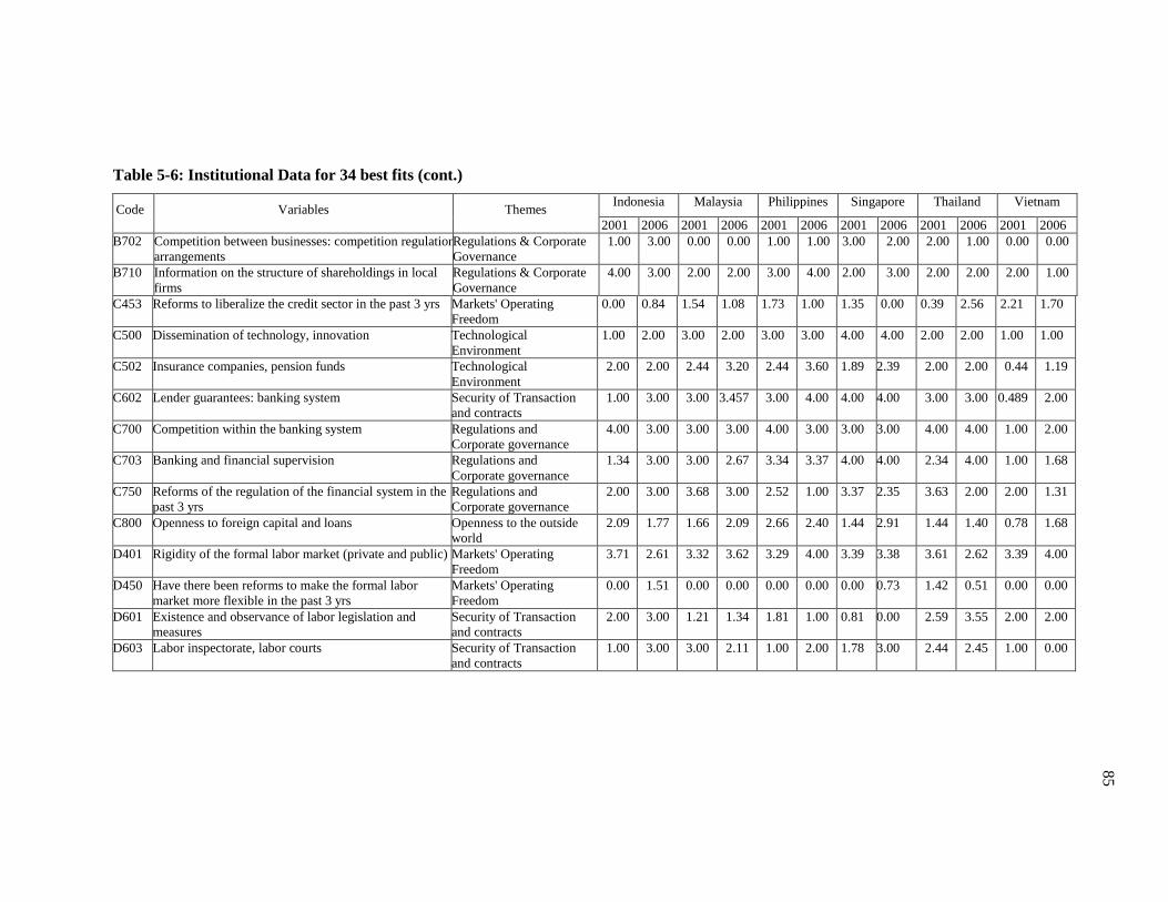
Table 5-6: Institutional Data for 34 best fits (cont.)

Code Variables Themes Indonesia Malaysia Philippines Singapore Thailand Vietnam

2001 2006 2001 2006 2001 2006 2001 2006 2001 2006 2001 2006

B702 Competition between businesses: competition regulation

arrangements

Regulations & Corporate

Governance

1.00 3.00 0.00 0.00 1.00 1.00 3.00 2.00 2.00 1.00 0.00 0.00

B710 Information on the structure of shareholdings in local

firms

Regulations & Corporate

Governance

4.00 3.00 2.00 2.00 3.00 4.00 2.00 3.00 2.00 2.00 2.00 1.00

C453 Reforms to liberalize the credit sector in the past 3 yrs Markets' Operating

Freedom

0.00 0.84 1.54 1.08 1.73 1.00 1.35 0.00 0.39 2.56 2.21 1.70

C500 Dissemination of technology, innovation Technological

Environment

1.00 2.00 3.00 2.00 3.00 3.00 4.00 4.00 2.00 2.00 1.00 1.00

C502 Insurance companies, pension funds Technological

Environment

2.00 2.00 2.44 3.20 2.44 3.60 1.89 2.39 2.00 2.00 0.44 1.19

C602 Lender guarantees: banking system Security of Transaction

and contracts

1.00 3.00 3.00 3.457 3.00 4.00 4.00 4.00 3.00 3.00 0.489 2.00

C700 Competition within the banking system Regulations and

Corporate governance

4.00 3.00 3.00 3.00 4.00 3.00 3.00 3.00 4.00 4.00 1.00 2.00

C703 Banking and financial supervision Regulations and

Corporate governance

1.34 3.00 3.00 2.67 3.34 3.37 4.00 4.00 2.34 4.00 1.00 1.68

C750 Reforms of the regulation of the financial system in the

past 3 yrs

Regulations and

Corporate governance

2.00 3.00 3.68 3.00 2.52 1.00 3.37 2.35 3.63 2.00 2.00 1.31

C800 Openness to foreign capital and loans Openness to the outside

world

2.09 1.77 1.66 2.09 2.66 2.40 1.44 2.91 1.44 1.40 0.78 1.68

D401 Rigidity of the formal labor market (private and public) Markets' Operating

Freedom

3.71 2.61 3.32 3.62 3.29 4.00 3.39 3.38 3.61 2.62 3.39 4.00

D450 Have there been reforms to make the formal labor

market more flexible in the past 3 yrs

Markets' Operating

Freedom

0.00 1.51 0.00 0.00 0.00 0.00 0.00 0.73 1.42 0.51 0.00 0.00

D601 Existence and observance of labor legislation and

measures

Security of Transaction

and contracts

2.00 3.00 1.21 1.34 1.81 1.00 0.81 0.00 2.59 3.55 2.00 2.00

D603 Labor inspectorate, labor courts Security of Transaction

and contracts

1.00 3.00 3.00 2.11 1.00 2.00 1.78 3.00 2.44 2.45 1.00 0.00

85

Table 5-7: A summary results in the database and its structure context

Institutional

themes in the

columns

Institutional

environment Markets

Institutional

themes in the row

-A- Public institutions,

Civil society

-B- Good and

services

-C- Capital market -D- Labor markets and

social relations

(1).Political

institutions

A100(+), A101(-),

A151(-), A102 (-),

A103(+)

(2).Safety, law and

order

A200(-)

(3).Public

governance

A350(+), A302(+),

A351(+)

A303(+), A304(+),

A305(-)

(4).Markets‘

operating freedom

B400(+), B451(-),

B452(-)

C453(+) D401(-), D450(+)

(5).Technological

environment,

Expectations

B500(-) C500(+), C502(-)

(6).Security of

transactions and

contracts

A600(+), A606(+),

A650(+)

B603(+), B604(+) C602(+) D601(+), D603(+)

(7).Regulations

and corporate

governance

B702(+), B710(-) C700(-), C703(+),

C750(+)

(8).Openness to

the outside world

A800(-) C800(-)

(9).Social

cohesion

C900(-)

Note: (+) and (-) denote statistically significant and positive, and negative, respectively. 86

87

5.6 Conclusion

In this chapter, we visit the impact of institutional ‗quality‘ on bilateral FDI in ASEAN during

1995 - 2005. The detailed Institutional Profile database is used to highlight the main institutions

that matter. We found that security of transactions and contracts have strong relation to increase

FDI inflow in ASEAN countries. These categories of institutions consist of security of traditional

property rights, law on bankruptcies, the security of transactions, the protection of intellectual

property, lender guarantees: banking system (mortgages etc), existence and observance of labor

legislation and measures, and labor inspectorate and labor courts. In addition, the results indicate

that good public governance has a positive relationship with FDI inflows. This category of

institutions covers transparency, corruption control, efficiency of administration, and

independence of the justice system. However we also find a negative relationship between good

institutions and FDI. These results do not imply that FDI flows would be increased by

institutional inefficiency. They only show that there is no direct positive effect of those

institutional variables on FDI.

88

5.7 Appendix

Table A5-1: -A- Public institutions and civil society

Code The Variable Names

1.Political Institutions

A100 Political rights and functioning of political institutions

A150 Evolution of political rights in the past 3 years

A101 Public freedoms and the autonomy of the civil society

A151 Evolution of freedoms and civil society autonomy in the past 3 years

A102 Concentration of the media

A103 Centralization - decentralization: devolution of local authorities

A104 Centralization - decentralization: autonomy in tax matters

2.Safety, law and order

A200 Internal public security

A201 External public security

A250 Evolution of the security in the past 3 years

3.Public governance

A300 Transparency of public action in the economic field

A301 Transparency of economic policy (fiscal, taxation, monetary, exchange-rate, etc)

A350 Evolution of transparency of public action in the past 3 years

A302 Corruption / Corruption

A351 Evolution of petty and large-scale corruption in the past 3 years

A303 Government-citizen relations

A352 Evolution in the effectiveness of public action as a whole in the past 3 years

A304 Effectiveness of public action: tax system

A353 Tax reforms in the past 3 years

A354 Evolution of the efficiency of the tax system in the past 3 years

A305 Running of the customs administration

A307 Running of the justice system

A355 Evolution of the independence and efficiency of the justice system in the past 3

years

A356 Public administration reforms in the past 3 years

5.Technological environment

A510 Capacity of the political authorities

A511 Society's aptitude for adaptation and innovation

A512 Long-term strategic vision of the authorities

A513 The authorities' strategies

A515 investment in the future of the population

6.Security of transactions and contracts

A600 Security of traditional property rights

A601 Security of property rights: formal property rights

A602 Form of contracts between private agents

89

A603 Security of contracts between private agents

A604 Government respect for contracts

A605 Settlement of economic disputes: justice in commercial matters

A606 Law on bankruptcies

A607 Application of law on bankruptcies

A650 Evolution of the security of transactions in the past 3 years

8.Openness to the outside world

A800 Free movement of persons, information, etc

A803 External pressure

9.Social cohesion

A900 equality of treatment: segregation based on traditions and beliefs

A901 Access without discrimination to healthcare and public and private employment

A902 Subsidies for primary products (social safety net)

A903 Traditional forms of solidarity

A904 Institutional solidarity

90

Table A5-2: -B- Goods and services

Code The Variable Names

3.Public governance

B300 Administrative business start-up formalities

4.Markets’ operating freedom

B400 Share of public sector in GDP

B403 Administered prices and market prices

B451 Implementation of the privatisation programme

B452 Openness of the privatisation programme

5.Technological environment

B500 Technological environment, dissemination of technology

6.Security of transactions and contracts

B600 Information on the situation of firms

B602 Information on the quality of the goods: international norms and standards

B603 Intellectual property

B604 Arrangements for the protection of intellectual property

7.Regulations and corporate governance

B700 Competition: productive sector: ease of market entry for new firms

B701 Competition in distribution (household consumption)

B702 Competition between businesses: competition regulation arrangements

B704 Interpenetration of local capital (private and/or public)

B710 Information on the structure of shareholdings in local firms

8.Openness to the outside world

B800 Convertibility and WTO membership

91

Table A5-3: -C- Capital Market

Code The Variable Names

4.Markets’ operating freedom

C400 Share of banking sector in private hands in 2001

C402 Level of government intervention in allocation of leading

C453 Reforms to liberalise the credit sector in the past 3 years

5.Technological Environment

C500 Dissemination of technology, innovation

C501 Innovation: venture capital

C502 Insurance companies, pension funds

6.Security of Transactions and Contracts

C600 Traditional credit systems (informal or quasi-informal)

C601 Information on the situation of the banks

C602 Lender guarantees: banking system (mortgages etc)

C603 Compulsory publication of information by firms at the time of share issues

7.Regulations and corporate governance

C700 Competition within the banking system

C702 Prudential rules: difference between local and international standards

C703 Banking and financial supervision

C704 Internal control of banks

C750 Reforms of the regulation of the financial system in the past 3 years

8.Openness to the outside world

C800 Openness to foreign capital and loans

C850 Reforms to open up the financial system in the past 3 years?

9.Social cohesion

C900 Micro-lending

92

Table A5-4: -D- Labor market and Social relations

Code The Variable Names

1.Political institutions

D100 Freedom of association

D101 Trade union plurality and autonomy

4.Markets’ operating

D401 Rigidity of the formal labor market (private and public)

D450 Have there been reforms to make the formal labor market more flexible in the past 3

years.

5.Technological environment

D500 Adult vocational training

6.Security of transactions and contracts

D600 Informal labor market

D601 Existence and observance of labor legislation and measures

D602 Employment contract protection

D603 Labor inspectorate, labor courts, etc

7.Regulations and corporate governance

D700 Wage bargaining for non-managerial staff

D701 Social dialogue

8.Openness to the outside world

D800 Openness to employment of foreign executives

9.Social cohesion

D900 Segmentation of the labor market

D901 Social mobility: Recruitment and promotion in the public and private sector

D902 Social mobility: Young graduates from higher education

D903 Child labor

D950 Have there been reforms aimed at de-segmentation of the labor market in the past 3

yrs?

Table A5-5: Estimates of Equation (5-3) with IP data

A100 A101 A103 A200 A350 A302 A351 A304 A305 A600 A606 A650

Home

GDP

0.648

(0.365)

0.651

(0.366)

0.644

(0.365)

0.647

(0.366)

0.648

(0.368)

0.644

(0.367)

0.648

(0.368)

0.647

(0.368)

0.643

(0.363)

0.646

(0.364)

0.650

(0.364)

0.652

(0.368)

Host

GDP

-2.519*

(1.012)

-0.882

(0.919)

3.182***

(0.953)

0.191

(0.869)

-0.443

(0.842)

-1.742

(0.904)

-2.082

(1.155)

-0.900

(0.838)

-0.696

(0.769)

-1.108

(0.757)

-0.0791

(0.825)

-0.829

(0.912)

Dist. -0.391**

(0.125)

-0.392**

(0.125)

-0.391**

(0.121)

-0.391**

(0.120)

-0.390**

(0.120)

-0.390**

(0.120)

-0.391**

(0.125)

-0.390**

(0.119)

-0.390***

(0.119)

-0.391**

(0.119)

-0.391**

(0.122)

-0.391**

(0.123)

Ex. 1.876**

(0.648)

0.915

(0.598)

2.393***

(0.615)

0.534

(0.545)

0.752

(0.542)

1.520**

(0.577)

1.454*

(0.690)

1.042

(0.539)

1.223*

(0.499)

1.321**

(0.491)

0.626

(0.521)

0.757

(0.569)

Op. -0.512

(0.486)

-0.314

(0.505)

-0.933

(0.501)

-0.941

(0.516)

-1.336*

(0.594)

-1.530**

(0.572)

-1.370*

(0.565)

-1.399*

(0.579)

-0.655

(0.504)

-0.493

(0.499)

-0.0981

(0.576)

-1.030

(0.539)

Tariff 0.369

(0.450)

0.835

(0.439)

0.121

(0.430)

0.359

(0.393)

0.279

(0.402)

-0.269

(0.443)

-0.394

(0.542)

0.208

(0.402)

0.557

(0.395)

1.050*

(0.447)

1.339*

(0.592)

0.588

(0.424)

Cor.

Tax

-3.568*

(1.513)

-2.613

(1.416)

-4.311**

(1.540)

-3.475*

(1.484)

-2.896*

(1.393)

-3.692*

(1.478)

-2.749

(1.471)

-3.232*

(1.422)

-4.656*

(1.553)

-3.777**

(1.441)

-2.860*

(1.386)

-2.060

(1.410)

Instit. 1.579***

(0.428)

-1.311*

(0.616)

2.248***

(0.479)

-0.890*

(0.395)

0.323*

(0.141)

1.135***

(0.328)

0.574***

(0.211)

0.994**

(0.361)

-1.307***

(0.361)

0.814***

(0.233)

0.544*

(0.257)

0.536*

(0.271)

R-sq 0.729 0.726 0.732 0.727 0.727 0.730 0.727 0.728 0.730 0.730 0.726 0.726

N 2204 2204 2204 2204 2204 2204 2204 2204 2204 2204 2204 2204

93

Table A5-5: Estimates of Equation (5-3) with IP data (Cont.)

A800 B451 B452 B500 B603 B702 B710 C500 C502 C602 C700 C703

Home

GDP

0.647

(0.367)

0.644

(0.363)

0.649

(0.367)

0.652

(0.367)

0.646

(0.368)

0.650

(0.366)

0.651

(0.369)

0.648

(0.367)

0.646

(0.367)

0.652

(0.367)

0.646

(0.362)

0.648

(0.367)

Host

GDP

-0.277

(0.830)

-0.768

(0.838)

-1.189

(1.161)

-1.008

(0.935)

-2.821*

(1.117)

-1.819

(0.933)

-1.224

(1.075)

-0.487

(0.805)

-0.755

(0.856)

-0.713

(0.855)

0.463

(0.905)

-0.292

(0.835)

Dist. -0.390**

(0.120)

-0.391**

(0.123)

-0.392**

(0.127)

-0.392**

(0.124)

-0.391**

(0.124)

-0.392**

(0.124)

-0.391**

(0.124)

-0.391**

(0.119)

-0.390**

(0.120)

-0.391**

(0.123)

-0.391**

(0.121)

-0.390**

(0.120)

Ex. 0.745

(0.535)

1.202*

(0.548)

1.104

(0.729)

0.887

(0.592)

1.919**

(0.676)

1.428*

(0.599)

0.928

(0.633)

0.791

(0.518)

0.978

(0.553)

0.740

(0.553)

0.546

(0.528)

0.682

(0.538)

Op. -1.217*

(0.557)

-0.277

(0.522)

-0.608

(0.494)

-0.677

(0.486)

-1.447**

(0.548)

-0.500

(0.485)

-1.211*

(0.590)

-1.107*

(0.534)

-1.376*

(0.574)

-0.738

(0.489)

0.0888

(0.614)

-1.263*

(0.581)

Tariff 0.271

(0.396)

0.187

(0.422)

-0.0513

(0.574)

0.694

(0.433)

-0.480

(0.506)

0.659

(0.434)

0.219

(0.476)

0.709

(0.412)

-0.065

(0.432)

0.825

(0.443)

1.102*

(0.498)

0.382

(0.395)

Cor.

Tax

-3.305*

(1.433)

-4.934**

(1.697)

-3.112*

(1.502)

-2.260

(1.415)

-3.275*

(1.516)

-2.992*

(1.460)

-2.074

(1.434)

-2.860*

(1.381)

-3.404*

(1.449)

-2.176

(1.399)

-4.123**

(1.580)

-2.888*

(1.388)

Instit. -0.773*

(0.316)

-1.113***

(0.311)

-0.881*

(0.412)

-0.967*

(0.450)

2.265***

(0.646)

0.561**

(0.178)

-0.453*

(0.223)

0.466*

(0.194)

-0.899**

(0.326)

0.393*

(0.192)

-0.703**

(0.258)

0.319*

(0.145)

R-sq 0.728 0.729 0.726 0.726 0.729 0.728 0.726 0.728 0.728 0.726 0.727 0.727

N 2204 2204 2204 2204 2204 2204 2204 2204 2204 2204 2204 2204

94

Table A5-5: Estimates of Equation (5-3) with IP data (Cont.)

C750 C800 D401 D450 D601 D603

Home

GDP

0.650

(0.367)

0.646

(0.363)

0.645

(0.366)

0.650

(0.366)

0.646

(0.367)

0.646

(0.364)

Host GDP -2.108

(1.093)

0.499

(0.901)

-0.590

(0.831)

-1.500

(0.942)

-1.058

(0.896)

-0.305

(0.778)

Distance -0.392**

(0.125)

-0.391**

(0.119)

-0.390**

(0.120)

-0.392**

(0.125)

-0.390**

(0.121)

-0.390***

(0.118)

Ex Rate 1.506*

(0.672)

0.490

(0.530)

0.962

(0.540)

1.235*

(0.605)

1.110

(0.575)

0.923

(0.490)

Openness -0.738

(0.489)

-0.420

(0.520)

-1.222*

(0.544)

-0.454

(0.486)

-1.416*

(0.572)

-0.619

(0.502)

Tariff 0.287

(0.472)

0.862

(0.443)

0.0288

(0.414)

0.700

(0.435)

-0.280

(0.464)

0.956*

(0.441)

Cor. Tax -2.843

(1.478)

-3.945*

(1.535)

-3.753*

(1.487)

-2.797

(1.444)

-3.401*

(1.459)

-3.861**

(1.455)

Instit. 0.559**

(0.190)

-0.876**

(0.338)

-0.532**

(0.185)

0.609**

(0.221)

0.720*

(0.247)

0.432**

(0.143)

R-sq 0.727 0.727 0.728 0.727 0728 0.729

N 2204 2204 2204 2204 2204 2204

95

Table A5-6: Estimates of Equation (5-4) with IP data

A100 A101 A103 A200 A350 A302 A351 A303 A304 A305 A600 A606

Home GDP 1.246*

(0.527)

1.237*

(0.532)

1.266*

(0.521)

1.267*

(0.525)

1.274*

(0.528)

1.282*

(0.525)

1.264*

(0.537)

1.268*

(0.532)

1.278*

(0.525)

1.269*

(0.514)

1.256*

(0.517)

1.237*

(0.524)

Host GDP -2.354*

(1.010)

-0.717

(0.914)

-3.078**

(0.953)

0.387

(0.866)

-0.282

(0.837)

-1.642

(0.895)

-1.955

(1.137)

-0.00791

(0.863)

-0.765

(0.833)

-0.528

(0.769)

-0.937

(0.762)

0.0847

(0.826)

Distance -0.400***

(0.120)

-0.399***

(0.120)

-0.401***

(0.117)

-0.400***

(0.115)

-0.401***

(0.115)

-0.401***

(0.116)

-0.401***

(0.120)

-0.401***

(0.116)

-0.401***

(0.114)

-0.400***

(0.114)

-0.400***

(0.114)

-0.399***

(0.117)

Sum of

GDP

-0.627

(0.399)

-0.621

(0.404)

-0.631

(0.393)

-0.634

(0.396)

-0.627

(0.398)

-0.636

(0.394)

-0.634

(0.404)

-0.624

(0.402)

-0.628

(0.396)

-0.636

(0.389)

-0.622

(0.392)

-0.618

(0.399)

Relat.

Factor

Endow.

0.557

(0.700)

0.423

(0.699)

1.036

(0.684)

0.916

(0.669)

1.216

(0.676)

1.270

(0.678)

0.818

(0.698)

1.109

(0.679)

1.313

(0.675)

1.021

(0.659)

0.956

(0.660)

0.524

(0.686)

Ex Rate 1.876**

(0.642)

0.905

(0.590)

2.467***

(0.615)

0.545

(0.539)

0.797

(0.536)

1.608**

(0.572)

1.486*

(0.681)

0.564

(0.553)

1.113*

(0.535)

1.264*

(0.492)

1.351**

(0.487)

0.622

(0.515)

Openness -0.467

(0.480)

-0.290

(0.498)

-0.839

(0.494)

-0.879

(0.513)

-1.299*

(0.586)

-1.470**

(0.562)

-1.316*

(0.551)

-1.225*

(0.611)

-1.348*

(0.571)

-0.557

(0.503)

-0.391

(496)

-0.0574

(0.564)

Tariff 0.389

(0.445)

0.847

(0.433)

0.141

(0.428)

0.372

(0.391)

0.282

(0.399)

-0.289

(0.440)

-0.395

(0.534)

0.389

(0.403)

0.213

(0.399)

0.590

(0.392)

1.102*

(0.441)

1.354*

(0.583)

Cor. Tax -3.577*

(1.495)

-2.615

(1.400)

-4.404**

(1.507)

-3.631*

(1.455)

-3.043*

(1.360)

-3.860**

(1.442)

-2.784

(1.451)

-2.544

(1.334)

-3.405*

(1.387)

-4.850**

(1.521)

-3.871**

(1.408)

-2.877*

(1.366)

Instit. 1.582***

(0.433)

-1.292*

(0.622)

2.334***

(0.481)

-0.952*

(0.392)

0.362*

(0.142)

1.226***

(0.326)

0.594**

(0.209)

0.302*

(0.151)

1.102**

(0.363)

-1.373***

(0.360)

0.844***

(0.232)

0.541*

(0.257)

R-sq 0.730 0.727 0.728 0.728 0.729 0.731 0.729 0.727 0.730 0.731 0.731 0.727

N 2204 2204 2204 2204 2204 2204 2204 2204 2204 2204 2204 2204

96

Table A5-6: Estimates of Equation (5-4) with IP data (cont.)

A650 A800 B400 B451 B452 B500 B603 B604 B702 B710 C453 C500

Home

GDP

1.255*

(0.536)

1.273*

(0.525)

1.269*

(0.532)

1.259*

(0.521)

1.249*

(0.535)

1.244*

(0.535)

1.270*

(0.532)

1.264*

(0.528)

1.242*

(0.529)

1.258*

(0.539)

1.266*

(0.528)

1.268*

(0.525)

Host

GDP

-0.710

(0.908)

-0.0962

(0.826)

-0.256

(0.864)

-0.630

(0.833)

-1.054

(1.146)

-0.840

(0.932)

-2.709*

(1.102)

0.0472

(0.828)

-1.647

(0.932)

-1.127

(1.061)

0.334

(0.877)

-0.316

(0.804)

Distanc

e

-0.401***

(0.118)

-0.400***

(0.115)

-0.401***

(0.116)

-0.399***

(0.119)

-0.399**

(0.123)

-0.400***

(0.120)

-0.401***

(0.120)

-0.401***

(0.115)

-0.400***

(0.120)

-0.401***

(0.119)

-0.400***

(0.116)

-0.401***

(0.114)

Sum of

GDP

-0.616

(0.407)

-0.631

(0.396)

-0.622

(0.402)

-0.648

(0.394)

-0.638

(0.403)

-0.618

(0.406)

-0.635

(0.401)

-0.619

(0.400)

-0.621

(0.401)

-0.621

(0.408)

-0.632

(0.399)

-0.620

(0.397)

Relat.

Factor

Endow.

0.912

(0.680)

1.144

(0.671)

1.168

(0.679)

0.515

(0.684)

0.345

(0.699)

0.628

(0.696)

0.960

(0.695)

1.127

(0.666)

0.571

(0.698)

0.885

(0.693)

0.933

(0.673)

1.220

(0.664)

Ex Rate 0.790

(0.565)

0.781

(0.528)

0.671

(0.549)

1.218*

(0.539)

1.106

(0.714)

0.889

(0.587)

1.972**

(0.668)

0.580

(0.526)

1.425*

(0.593)

0.970

(0.628)

0.493

(0.554)

0.835

(0.511)

Openne

ss

-0.987

(0.532)

-1.162*

(0.551)

-1.282*

(0.613)

-0.235

(0.517)

-0.592

(0.488)

-0.622

(0.482)

-1.381*

(0.537)

-0.988

(0.535)

-0.453

(0.479)

-1.172*

(0.577)

-1.020

(0.544)

-1.033

(0.529)

Tariff 0.618

(0.420)

0.278

(0.394)

0.395

(0.403)

0.195

(0.418)

-0.0415

(0.565)

0.718

(0.427)

-0.481

(0.500)

0.809

(0.423)

0.679

(0.428)

0.221

(0.471)

0.290

(0.404)

0.764

(0.409)

Cor.

Tax

-2.078

(1.394)

-3.482*

(1.400)

-2.474

(1.341)

-5.007**

(1.677)

-3.116*

(1.489)

-2.275

(1.398)

-3.330*

(1.490)

-2.634*

(1.328)

-3.001*

(1.442)

-2.089

(1.421)

-3.175*

(1.399)

-2.987*

(1.348)

Instit. 0.584*

(0.266)

-0.847**

(0.317)

0.564*

(0.262)

-1.131***

(0.310)

-0.880*

(0.413)

-0.975*

(0.449)

2.351***

(0.642)

0.483*

(0.223)

0.561*

(0.180)

-0.489*

(0.219)

0.251*

(0.119)

0.516**

(0.196)

R-sq 0.727 0.727 0.728 0.730 0.727 0.727 0.731 0.728 0.729 0.727 0.727 0.729

N 2204 2204 2204 2204 2204 2204 2204 2204 2204 2204 2204 2204

97

Table 5-5: Estimates of Equation (5-4) with IP data (cont.)

C502 C602 C700 C703 C750 C800 D401 D450 D601 D603

Home

GDP

1.277*

(0.526)

1.247*

(0.534)

1.245*

(0.519)

1.272*

(0.527)

1.246*

(0.534)

1.257*

(0.519)

1.276*

(0.523)

1.240*

(0.531)

1.276*

(0.528)

1.262*

(0.516)

Host GDP -0.603

(0.851)

-0.554

(0.857)

0.611

(0.899)

-0.116

(0.831)

-1.940

(1.085)

0.691

(0.898)

-0.427

(0.828)

-1.329

(0.940)

-0.921

(0.889)

-0.112

(0.780)

Distance -0.401***

(0.115)

-0.400***

(0.118)

-0.398***

(0.116)

-0.401***

(0.115)

-0.400***

(0.121)

-0.399***

(0.115)

-0.400***

(0.115)

-0.400***

(0.120)

-0.401***

(0.117)

-0.400***

(0.113)

Sum of

GDP

-0.635

(0.396)

-0.616

(0.405)

-0.633

(0.395)

-0.626

(0.398)

-0.625

(0.404)

-0.633

(0.394)

-0.637

(0.394)

-0.621

(0.403)

-0.638

(0.397)

-0.626

(0.391)

Relat.

Factor

Endow.

1.140

(0.675)

0.750

(0.684)

0.449

(0.683)

1.196

(0.674)

0.571

(0.704)

0.755

(0.663)

1.096

(0.672)

0.512

(0.699)

1.059

(0.679)

1.027

(0.654)

Ex Rate 1.028

(0.547)

0.751

(0.549)

0.547

(0.520)

0.720

(0.531)

1.504*

(0.665)

0.493

(0.523)

1.004

(0.534)

1.229*

(0.598)

1.158*

(0.568)

0.949*

(0.484)

Openness -1.326*

(0.565)

-0.672

(0.486)

0.124

(0.603)

-1.221*

(0.574)

-0.692

(0.483)

-0.345

(0.518)

-1.161*

(0.537)

-0.415

(0.481)

-1.366*

(0.561)

-0.515

(0.502)

Tariff -0.0809

(0.429)

0.860*

(0.436)

1.119*

(0.491)

0.396

(0.393)

0.307

(0.467)

0.896*

(0.438)

0.0242

(0.412)

0.718

(0.429)

-0.301

(0.459)

1.012*

(0.437)

Cor. Tax -3.569*

(1.416)

-2.198

(1.381)

-4.159**

(1.559)

-3.035*

(1.356)

-2.850

(1.460)

-4.065**

(1.506)

-3.939**

(1.454)

-2.802*

(1.427)

-3.536*

(1.426)

-4.010**

(1.422)

Instit. -0.975**

(0.324)

0.408*

(0.190)

-0.707*

(0.257)

0.358*

(0.146)

0.560**

(0.191)

-0.906**

(0.334)

-0.572**

(0.184)

0.606**

(0.223)

0.771**

(0.244)

0.455**

(0.142)

R-sq 0.729 0.727 0.728 0.729 0.729 0.729 0.730 0.728 0.729 0.730

N 2204 2204 2204 2204 2204 2204 2204 2204 2204 2204

98

99

Bibliography

Aitken, N. D. (1973). The Effect of the EEC and EFTA on European Trade: a Temporal Cross

Section Analysis. American Economic Review, 63, 881-892.

Aizenman, J., & Spiegel, M. M. (2006). Institutional Efficieny, Monitoring Costs, and the

Investment Share of FDI. Review of International Economics, 14(4), 683-697.

Al-Atrash, H., & Yousef, T. (2000). Intra-Arab Trade: Is it Too Little. IMF Working

Paper(WP/00/10).

Amjadi, A., & Yeats, A. J. (1995, December). Have Transport Costs Contributed to the Relative

Decline of Sub-Saharan African Exports? Some Preliminary Empirical Evidence. The

World Bank, International Economics Department. Washington D.C.: International Trade

Division.

Anderson, J. E. (1979). A Theoretical Foundation for the Gravity Equation. American Economic

Review(69), 106-116.

Anderson, J. E., & van Wincoop, E. (2003, Mar.). Gravity with Gravitas: ASolution to the Border

Puzzle. The American Economic Review, 93(1), 170-192.

Anderson, J. E., & Wincoop, E. v. (2004, September). Trade Costs. Journal of Economic

Literature, 42(3), 691-751.

Asiedu, E. (2006). Foreign Direct Investment in Africa: The role of Natural Resources, Market

Size, Government Policy Instability. The World Economy, 29(1), 63-77.

Baier, S. L., & Bergstrand, J. H. (2001). The growth of world trade: tariffs, transport costs, and

income similarity. Journal of International Economics, 53, 1-27.

Baltagi, B. H., Egger , P., & Pfaffermayr, M. (2003). A generalized design for bilateral trade flow

models. Economics Letters, 80(3), 391-397.

Bank, A. D. (2006). Asian Development Outlook. Asian Development Bank.

Bayoumi, T., & Eichengreen, B. (1995). Is regionalism simply a diversion? Evidence from the

evolution of the EC and EFTA. CEPR Discussion Paper No.1294.

Benassy-Quere, A., Coupet, M., & Mayer, T. (2007). Institutional Determinants of Foreign Direct

Investment. The World Economy, 30(5), 764-782.

Bergeijk, P. A., & Brakman, S. (2010). Introduction: the comback of the gravity equation. In P.

Bergeijk, & S. Brakman, The gravity model in international trade: advances and

applications. Cambridge University Press.

Bergstrand , J. H. (1985). The Gravity Equation in International Trade: Some Microeconomic

Foundations and Empirical Evidence. Review of Economics and Statistics, 67(3), 475-81.

100

Bergstrand , J. H. (1989). The Generalized Gravity Equation, Monopolistic Competition, and

Factor Proportions Theory in International Trade. Review of Economics and Statistics,

71(1), 143-53.

Bhagwati , J., & Panagariya, A. (1996). The Economics of Preferential Trade Agreement.

Washington DC.: AEI Press.

Bhagwati, J., & Krueger, A. (1995). The Dangerous Drift to Preferntail Trade Agreements.

Washington DC.: AEI Press.

Blonigen, B. A. (2005). A Review of the Empirical Literature of FDI Determinants. Atlantic

Economic Journal, 33, 383-403.

Busse , M. (2003). Tariffs, Transport Costs and the WTO Doha Round: The Case of Developing

Countries. The Estey Center Journal of International Law and Trade Policy, 4(1), 15-31.

Carrère, C. (2004). African Regional Agreements: Impact on Trade with or without Currency

Unions. Journal of African Economies, 13(2), 199-239.

Carrere, C. (2006). Revisiting the Effects of Regional Trade Agreements on Trade Flows with

Proper Specification of the Gravity Model. European Economic Review, 50, 223-247.

Caves, R. E. (1996). Multinational Enterprise and Economic Analysis (Second ed.). NY:

Canbridge University Press.

Cernat , L. (2001). Assessing Regional Trade Arrangements: Are South-South RTAs More Trade

Diverting? Global Economy Quarterly, 2, 235-260.

Cheng , I.-H., & Wall, H. J. (2005, January/February). Controlling for Heterogeneity in Gravity

Models of Trade and Integration. Federal Reserve Bank of St.Louis Review, 87(1), 49-63.

Clark, D. P. (2007). Distance, Production, and Trade. Journal of International Trade and

Economic Development, 16(3), 359-371.

Clark, X., Dollar, D., & Micco, A. (2004). Port efficiency, maritime transport costs and bilateral

trade. Journal of Development Economics, 75, 417-450.

Coe, D., & Hoffmaister, A. (1999). Norht-South Trade: Is Africa Unusual? Journal of Afircan

Economies, 8(2), 228-256.

Combes, P. P., & Lafourcade, M. (2005). Transport costs: Measures, determinants and regional

policy implications for France. Journal of Economic Geography, 5(3), 319-349.

Croce, E., Juan-Ramon, V. H., & Zhu, F. (2004, June). Performance of Western Hemisphere

Trading Blocs: A Cost-Corrected Gravity Approach. IMF Working Paper(WP/04/109).

Dauae, C., & Stein, E. (2007). The Quality of Institutions and Foreign Direct Investment.

Economics and Politics, 19(3), 317-344.

101

Daude, C., & Stein, E. (2007, November). The Quality of Institutions and Foreign Direct

Investment. Economics and Politics, 19(3), 317-344.

Deardorff, A. V. (1998). Determinants of bilateral trade: does gravity work in a neoclassical

world? In J. A. Frankel, The Regionalization of the World Economy. Chicago: University

of Chicago Press.

Dee, P., & Gali, J. (2005). The Trade and Investment Effects of Preferential Trading

Arrangements. In T. Ito, & A. K. Rose, International Trade in East Asia (pp. 133-176).

University of Chicago Press.

Deltas, G., Desmet, K., & Facchini, G. (2006). Hub-and-Spoke Free Trade Areas. CEPR

Discussion Paper, No. 5960.

Desbordes, R., & Vicard, V. (2009). Foreign direct investment and bilateral investmnet treaties:

An international political perspective. Journal of Comparative Economic, 37(3), 372-386.

di Giovanni, J. (2005). What drives capital flows? The case of cross-border activity and financial

deepening. Journal of International Economics, 65, 127-49.

Eaton, J., & Tamura, A. (1994). Bilateralism and Regionalism in Japanese and US Trade and

Direct Foreign Investment Patterns. Journal of the Japanese and International

Economics, 8, 478-510.

Egger, P. (2005). On the impact of transportation costs on trade in a mulilateral world. Southern

Economic Journal, 71(3), 592-606.

Elliott, R. J., & lkemoto, K. (2004). AFTA and the Asian Crisis: Help or Hindrance to ASEAN

Intra-Regional Trade? Asian Economic Journal, 18(1), 1-23.

Endoh, M. (1999). Trade creation and trade diversion in the EEC, the LAFTA and the CMEA:

1960-1994. Applied Economics, 31, 207-216.

Endoh, M. (2000). The Transition of Postwar Asia-Pacific Trade Relations. Journal of Asian

Economics, 10, 571-587.

Ethier, W. J. (1998). The new regionalism. The Economic Journal, 108, 1149-1161.

Evenett , S. J., & Keller, W. (2002, April). On Theories Explaining the Success of the Gravity

Equation. The Journal of Political Economiy, 110(2), 281-316.

Feenstra, R. C. (2004). Advance International Trade: Theory and Evidence. Princeton, NJ:

Princeton University Press.

Foroutan, F., & Pritchett, L. (1993). Intra-Sub-Saharan African Trade: Is It Too Little? Journal of

African Economies, 74-105.

Frankel , J. A. (1997). Regional Trading Blocs in the World Economic System. Washington, DC.:

Institute for International Economics.

102

Geraci , V. J., & Prewo, W. (1977). Bilateral Trade Flows and Transport Costs. The Review of

Economics and Statistics, 59(1), 67-74.

Globerman, S., & Shapiro, D. (2002). Global Foreign Direct Investmnet Flows: The Role of

Governance Infrastructure. World Development, 30(11), 1899-1919.

Globerman, S., & Shapiro, D. (2003). Governance infrastructure and US foreign direct

investmnet. Journal of International Business Studies, 34(1), 19-39.

Grossman, G. M. (1998). Comment. In J. A. Frankel, The Regionalization of the World Economy

(pp. 29-31). Chicago, IL: University of Chicago Press.

Gujarati, D. N. (2002). Basic Econometrics. (4, Ed.) McGraw-Hill/Irwin.

Halvorsen, R., & Palmquist, R. (1980). The interpretation of dummy variables in semilogarithmic

equations. American Economic Review, 70(3), 474-475.

Hamilton, C. B., & Winters, L. A. (1992). Opening up international trade with Eastern Europe.

Economic Policy, 14, 77-116.

Harrigan, J. (2003). Specialization and the volume of trade: do the data obey the laws? In K.

Choi, & J. Harrigan, The Handbook of International Trade. New York: Basil Blackwell.

Hausmann, R., & Fernandez-Arias, R. (2000). Foreign Direct Investment: Good Cholesterol?

Annual Meeting of the Board of Governors, Inter-American Development Bank and Inter-

American Investment Corporation. Inter-american Development Bank.

Helpman, E., & Krugman, P. R. (1985). Market Structure and Foreign Trade; Increasing

Returns, Imperfect Competition and the International Economy. Cambridge: MIT Press.

Helpman, E., Melitz, M., & Rubinstein, Y. (2008, May). Estimating Trade Flows: Trading

Partners and Trading Volumes. Quarterly Journal of Economics, CXXIII(2), 441-487.

Herrera , E. G. (2010, September). Retrieved November 12, 2010, from

http://www.ugr.es/~teoriahe/RePEc/gra/wpaper/thepapers10_05.pdf

Hummels, D. (2000). Have International Transportation Costs Declined?

Hummels, D. (2007). Transportation Costs and International trade in the Second Era of

Globalizaiton. The Journal of Economic Perspectives, 21(3), 131-154.

Hummels, D., & Lugovskyy, V. (2006). Are Matched Partner Trade Statistics a Usable Measure

of Transportation Costs? Review of International Economics, 14(1), 69-86.

Jacks, D. S., & Pendakur, K. (2010, November). Global Trand and the Maritime Transport

Revolution. The Review of Economics and Statistics, 92(4), 745-755.

Jacks, D. S., Meissner, C. M., & Novy, D. (2008). Trade Costs, 1870-2000. American Economic

Review: Papers & Proceedings, 98(2), 529-534.

103

Johnson, H. G. (1962). Money, Trade and Economic Growth: Survey Lectures in Economic

Theory. London: George Allen and Unwin.

Kaufman, D., Kraay, A., & Zoido-Lobaton, P. (1999). Aggregating Governance Indicators. World

Bank Working Paper, 2195.

Kaufman, D., Kraay, A., & Zoido-Lobaton, P. (1999). Governance Matters. World Bank Working

paper , 2196.

Kaufmann, D., Kraay, A., & Mastruzzi, M. (2009). Governance Matters VII: Governance

Indicators for 1996-2008. World Bank Policy Research.

Kepaptsoglou, K., Karlaftis, M. G., & Tsamboulas, D. (2010). The Gravity Model Specification

flor Modeling Internaitonal Trade Flows and Free Trade Agreement Effects: A 10-Year

Review of Empirical Studies. The Open Economics Journal, 3, 1-13.

Kien, N. T., & Hashimoto, Y. (2005). Economic Analysis of ASEAN Free Trade Area-By A

Country Panel Data. Retrieved December 2010, from http://www2.econ.osaka-

u.ac.jp/library/global/dp/0512.pdf

Kleinert , J., & Toubal, F. (2010). Gravity for FDI. Review of International Economics, 18(1), 1-

13.

Krugman, P. (1993). Regionalism versus multilateralism: Analytical notes. In J. De Melo, & A.

Panagariya, New Dimensions in Regioanl Integration (pp. 58-80). Cambridge: Cambridge

University Press.

Kuwamori, H. (2006, May). The Role of Distance in determining International Transport Costs:

Evidence from Philippine Impact Data. Institute of Developing Economies. Japan

External Trade Organization.

La Porta, R., Lopez-de-Silanes, & Vishny, R. (1998). The Quality of Government. NBER

Working Paper, 6727.

La Porta, R., Lopez-deSilanes, F., & Vishny, R. (1997). Legal Determinants of External Finance.

Journal of Finance, 52(3), 1131-1150.

Limao, N., & Venables, A. (2001). Infrastructure, grographical disadvantage, trapsort costs and

trade. The World Bank Economic Review, 15(3), 451-479.

Markusen, J. R., & Maskus, K. E. (2002). Discriminating Among Alternative Theories of The

Multinational Enterprise. Review of International Economics, 10(4, Nov), 695-707.

Martinez-Zarzoso , I., & Suarez-Burguet, C. (2005). Transport Costs and Trade: Empirical

Evidence for Latin American Imports from the European Union. Journal of Trade and

Economic Development, 14(3), 353-371.

104

Martinez-Zarzoso, I., & D., F. N.-L. (2007). Is Distance a Good Proxy for Transport Costs?: The

Case of Competing Transport Modes. Journal of International Trade & Economic

Development, 16(3), 411-434.

Matyas, L. (1997). Proper econometric specification of the gravity model. The World Economy,

20, 262-302.

Meisel, N., & Aoudia, J. O. (2007, September). A new institutional database: Institutional

Profiles 2006. DGTPE Working Papers.

Micco, A., & Perez, N. (2002). Determinants of Maritime Transport Costs. Inter-American

Development Bank.

Mishra, A., & Daly, K. (2007, June). Effect of Quality of Institutions on Outward Foreign Direct

Invesment. Journal of International Trade and Economic Development, 16(2), 231-244.

Naude, W. A., & Krugell, W. F. (2007). Investigating geography and institutions as determinants

of foreign direct investment in Africa using panel data. Applied Economics, 39, 1223-

1233.

Nijman, T., & Verbeck, M. (1992). Incomplete Panels and Selection Bias. In The Econometrics of

Panel Data: Handbook of Theory and Applications (pp. 262-302). Dordrecht: Kluwer

Academic Publishers.

North, D. C. (1987). Institutions, Transactions Costs and Economic Growth. Economic Inquiry,

25(3), 419-428.

Nowak-Lehmann, F., Herzer, D., Martinez-Zarzoso, I., & Vollmer, S. (2007). The Impact of a

Customs Union between Turkey and the EU on Turkey's Exports to the EU. Journal of

Common Market Studies, 45(3), 719-743.

Oguledo, V. I., & MacPhee, C. R. (1994). Gravity Models: A Reformulation and an Application

to Discriminatory Trade Arrangements. Applied Economics, 26(2), 107-20.

Radelet, S., & Sachs, J. (1998, January 1). Shipping Costs, Manufactured Exports and Economic

Growth. Retrieved December 5, 2010, from The Earth Institute, Columbia University:

http://admin.earth.columbia.edu/sitefiles/file/about/director/pubs/shipcost.pdf

Ramsey, J. B. (1969). Tests for Specification Errors in Classical Linear Least Squares Regression

Analysis. Journal of the Royal Statistical Society. Series B (Methodological), 31(2), 350-

371.

Redding, S., & Venables, A. J. (2000). Economic Geography and International Inequality. CEPR

Discussion Paper 2568.

Rivera-Batiz, L. A., & Oliva, M.-A. (2003). International trade: theory, strategies, and evidence.

USA: Oxford University Press.

105

Rose, A. K., & van Wincoop, E. (2001). National Money as a Barrier to International Trade: The

Real Case for Currency Union. American Economic Review, 91(2), 389-390.

Sanchez, R. J., Hoffmann, J., Micco, A., Pizzolitto, G. V., Sgut, M., & Wilmsmeier, G. (2003).

Port Efficiency and International Trade: Port Efficiency as a Determinant of Maritime

Transport Costs. Maritime Economics & Logistics, 5, 199-218.

Siliverstovs, B., & Schumacher, D. (2009). Estimating gravity equations: to log or not to log?

Empir Econ, 36, 645-669.

Silva, J. S., & Tenreyro, S. (2006). The Log of Gravity. Review of Economics and Statistics,

88(4), 641-658.

Soloaga, I., & Winters, L. A. (2001). How Has Regionalism in the 1990s Affected Trade? North

American Journal of Economics and Finance, 12, 1-29.

Soloaga, I., & Winters, L. A. (2001). Regionalism in The Nineties: What Effect on Trade? The

North American Journal of Economics and Finance, 12, 1-29.

Srinivasan , T. (1998). Developing Countries and the Multilateral Tradeing System. Boulder,

CO.: Westview Press.

StataCorp. (2009). Stata Statistical Software: Release 11. College Station, TX: StataCorp LP.

Talbott, J., & Roll, R. W. (2001, November 13). Why Many Developing Countries Just Aren't.

Retrieved December 15, 2010, from Social Science Research Network:

http://www.cipe.org/programs/roundtables/webevents/pdf/talbot.pdf

Tang, D. (2005, June). Effects of the Regional Trading Arrangements on Trade: Evidence from

the NAFTA, ANZCER and ASEAN Countries, 1989-2000. Journal of Trade and

Economic Development, 14(2), 241-265.

Tanzi, V., & Davoodi, H. (1997, October). Corruption, Public Investment, and Growth. IMF

Working Paper, WP/97/139.

The World Bank . (2001). Global Economic Prospects and the Developing Countries 2002:

Making Trade Work for the Poor. Washington, D.C.

The World Bank. (2004). Trade Policies in South Asia: An Overview (In Three Volumes) Volume

ll: An Overview. Washington, D.C.: The World Bank.

Tinbergen, J. (1962). Shaping the world economy: Suggestions for an international economic

policy. New York: Twentieth Century Fund.

Trotignon, J. (2010, June). Does Regional Integration Promote the Mulitilateralization of Trade

Flows? A Gravity Model Using Panel Data. Journal of Economic Integration, 25(2), 223-

251.

106

Tumbarello, P. (2007, March). Are Regional Trade Agreements in Asia Stumbling or Building

Blocks? Implications for the Mekong-3 Countries. IMF Working Paper.

UNCTAD. (2003). Review of Maritime Transport, 2003. New York and Geneva: United Nations.

Uttama, N. P., & Peridy, N. (2009). The Impact of Regional Integration and Third-Country

Effects on FDI: Evidence from ASEAN. ASEAN Economic Bulletin, 26(3), 239-252.

Van den Berg, H. (2001). Economic Growth and Development (1 ed.). McGraw-Hill/Irwin.

Van den Berg, H., & Lewer, J. J. (2006). International Trade and Economic Growth.

M.E.Sharpe.

Viner, J. (1950). The Customs Union Issue. New York: Carnegie Endowment for International

Peace.

Waczing , R., & Welch, K. H. (2008). Trade Liberalization and Growth: New Evidence. World

Bank Econ Rev, 22(2), 187-231.

Wooldridge , J. M. (2001). Econometric Analysis of Cross Section and Panel Data. The MIT

Press.

WTO. (2004). World Trade Report 2004 Exploring the linkage between the domestic policy

environment and international trade.

WTO. (2010). International Trade Statistics 2010. World Trade Organization.