Essays on Labor and Development Economics

Ashna Arora

Submitted in partial fulfillment of the

requirements for the degree of

Doctor of Philosophy

in the Graduate School of Arts and Sciences

COLUMBIA UNIVERSITY

2018

c� 2018

Ashna Arora

All rights reserved

ABSTRACT

Essays on Labor and Development Economics

Ashna Arora

This dissertation studies the impact of institutional interventions on labor markets in the United

States, Norway and India. The labor markets studied are diverse, and include the criminal sector

in the United States, the healthcare sector in Norway and the market for workfare employment in

rural India.

Chapter 1 studies whether juvenile o↵enders are deterred by the threat of criminal sanctions.

Existing research, which studies adolescent crime as a series of on-the-spot decisions, finds that

deterrence estimates are negligible at best. This paper first presents a model that allows the

return from crime to increase with previous criminal involvement. The predictions of the model are

tested using policy variation in the United States over the period 2006-15. The results show that

when criminal capital accumulates, juveniles may respond in anticipation of increases in criminal

sanctions. Accounting for these anticipatory responses can overturn the conclusion that harsh

sanctions do not deter juvenile crime.

Chapter 2 studies the impact of a graduate’s first job on her career trajectory, and how job-

seeking graduates respond to the persistence of these “first job e↵ects”. For identification, we

exploit a natural experiment in Norway, where doctors’ first jobs were allocated through a random

serial dictatorship mechanism until 2013. We use administrative data on individual outcomes to

confirm empirically that the residency allocation mechanism e↵ectively randomized choice sets of

hospitals across medical graduates. We then use the resulting variation in individual doctors choice

sets to show that first jobs a↵ect doctors’ earnings, place of residence, and specialization in the

long run.

Chapter 3 evaluates the e↵ects of encouraging the selection of local politicians in India via

community-based consensus, as opposed to a secret ballot election. I find that financial incentives

aimed at encouraging consensus-based elections and discouraging political competition crowd in

younger, more educated political representatives. However, these incentives also lead to worse gov-

ernance as measured by a fall in local expenditure and regressive targeting of workfare employment.

These results can be explained by the fact that community-based processes are prone to capture

by the local elite, and need not improve the quality of elected politicians or governance.

Table of Contents

List of Figures ii

List of Tables iv

Acknowledgements vi

Dissertation Committee vii

Chapter 1 Juvenile Crime and Anticipated Punishment 1

1 Introduction 2

2 Setting and Data 8

3 Theoretical Framework 15

4 Empirical Strategy 26

5 Results 28

6 Conclusion 37

7 References 38

8 Appendix 56

Chapter 2 The Career Impact of First Jobs: Evidence and Labor

Market Design Lessons from Randomized Choice Sets 65

1 Introduction 66

2 Setting 68

3 Data 71

4 Empirical Strategy 73

5 Results 77

6 Conclusion 83

7 References 84

8 Appendix 95

i

Chapter 3 Election by Community Consensus: E↵ects on Political

Selection and Governance 105

1 Introduction 106

2 Setting and Data 109

3 Empirical Strategy 117

4 Results 120

5 Conclusion 133

6 References 134

7 Appendix 138

ii

List of Figures

Chapter 1

Saddle Path Under Age-Independent Sanctions 20

Criminal Capital Accumulation Under Anticipated Adult Sanctions 21

ct And kt Under Anticipated Adult Sanctions 22

Response To An Increase In T 24

Crime Response To An Increase In T 25

Crime Reporting Increases At Age Of Criminal Majority

Proportion Of Arrests By Age 2006-14 43

Gang Membership-Age Profile 44

Criminal Involvement-Age Profile 45

Impact Of An Increase In The Age Of Criminal Majority

On O↵enses Related To Street Gangs 46

Impact Of An Increase In The Age Of Criminal Majority

On O↵enses Related To Street Gangs (Crime Index) 47

Impact Of An Increase In The Age Of Criminal Majority

17-Year Olds Versus 13-16 Year Olds 48

Juvenile And Adult Arrest Rates 1980-2014 57

Proportion Of O↵enses By Age 2006-14 58

Criminal Capital Accumulation Under Anticipated Adult Sanctions 59

ct And kt Under Anticipated Adult Sanctions 59

Age Profiles Of Gang Membership And Criminal Involvement 60

Chapter 2

Number Of Individuals And Hospitals By Lottery 86

Doctor Observations Post-Residency 86

First Stage Refinements 87

Long-Run E↵ects 88

Decomposing FJEs 89

iii

Lottery Participants By Gender And Country Of Birth 95

Number Of Residency Options For Lottery Participants 95

Number Of Hospitals And Hospital Size Over Time 96

Returns To Specialization 97

Alternative First Stage Refinements 98

Long-Run E↵ects: Demographic Heterogeneity 99

Chapter 3

Number Of Seats Increase With GP Population 111

Electoral Competition 122

Candidate & Politician Selection E↵ects 125

Gp Expenditure & Income 128

Workfare Employment: Creation And Targeting 131

Council Member Reservations & GP Population 139

Distribution Of GP Population 140

iv

List Of Tables

Chapter 1

Impact Of An Increase In The Age Of Criminal Majority On Juveniles Aged 13-17 49

Impact By Age Group 50

Impact By O↵ense Type: O↵enses Related To Street Gangs 51

Impact By O↵ense Type: Other O↵enses 52

Impact Of Acm Increase On Gang-Related Crime Index By Demographic Group 53

Social Costs Of Increase In Juvenile O↵ending 54

Seventeen Year Olds: Change In Annual Cost Of Incarceration 55

States Age Of Criminal Majority Over Time 61

Jurisdictions Bordering Treatment And Control States 62

Robustness Checks: Impact Of An Increase In The Age Of Criminal Majority On The

Juvenile Arrest Rate For Gang Related O↵enses 63

Robustness Checks: Impact Of An Increase In The Age Of Criminal Majority On The

Juvenile Crime Index For Gang Related O↵enses 64

Chapter 2

Hospital Characteristics 90

Doctor Characteristics 91

Randomization Via Lottery 92

Preferences (MRS) For Hospital Characteristics: Male X Norwegian X Rural 93

Preferences (MRS) For Long-Term Hospital Characteristics 94

Correlation Across Hospital Characteristics 96

Salary Variation With Firm And Individual Characteristics 100

Preferences For Hospital Characteristics: Male X Norwegian X Rural 101

Long-Term Hospital Salary 102

Long-Term Specialization 103

Long-Term Rural Location 104

v

Chapter 3

Samras Incentive Amounts By GP Type 114

E↵ects On Electoral Competition 123

E↵ects On Candidate Pool 126

E↵ects On Politician Identity 127

E↵ects On Income And Expenditure 129

E↵ects On Employment Creation And Targeting 132

Baseline Covariates: Demographics & Public Goods 141

Rule Based E↵ects: Council Size And Reservations For Women 142

E↵ects Of Additional Members On Electoral Competition 142

E↵ects Of Additional Members On Candidate Pool 142

E↵ect Of Additional Members On Politician Identity 143

E↵ects Of Additional Members On Income And Expenditure 143

E↵ects Of Additional Members On Employment Creation 144

vi

Acknowledgements

I am deeply indebted to my advisors Suresh Naidu and Bernard Salanie for being exceptionally

generous with their time, and for passing on their infectious enthusiasm for research. I am also

grateful for the advice, insight and support provided by Francois Gerard, Jonas Hjort and Rodrigo

Soares throughout the process of writing this dissertation.

This dissertation was vastly improved by insightful comments and discussions with Pierre-Andre

Chiappori, Christopher Cotton, Kunjal Desai, Siddharth Hari, Nandita Krishnaswamy, Aditya Ku-

valekar, Sun Kyoung Lee, Nikhil Patel, Lorenzo Pessina, Cristian Pop-Eleches, Daniel Rappoport,

Miikka Rokkanen, Christoph Rothe, Divya Singh, Miguel Urquiola, Eric Verhoogen, Scott Weiner,

Danyan Zha and Jonathon Zytnick.

Finally, I thank my family for their abundance of (over)confidence in me.

vii

Dissertation Committee

Suresh Naidu

Department of Economics and School of International and Public A↵airs

Columbia University

Bernard Salanie

Department of Economics

Columbia University

Francois Gerard

Department of Economics

Columbia University

Jonas Hjort

Graduate School of Business

Columbia University

Rodrigo Soares

School of International and Public A↵airs

Columbia University

viii

Chapter 1

Juvenile Crime and Anticipated Punishment⇤

Ashna Arora†

Abstract

Are juvenile offenders deterred by the threat of criminal sanctions? Recent research suggests

that they are not. This conclusion is based on the finding that criminal behavior decreases only

marginally as individuals cross the age of criminal majority, the age at which they are trans-

ferred from the juvenile to the more punitive adult criminal justice system. Using a model of

criminal capital accumulation, I show theoretically that these small reactions close to the age

threshold mask larger responses away from, or in anticipation of, the age threshold. I exploit

recent policy variation in the United States to show evidence consistent with this prediction -

arrests of 13-16-year-olds rise significantly for offenses associated with street gangs, including

drug, homicide, robbery, theft, burglary and vandalism offenses, when the age of criminal ma-

jority is raised from seventeen to eighteen. In contrast, and consistent with previous work, I

find that arrests of 17-year-olds do not increase systematically in response. I provide sugges-

tive evidence that this null effect is likely due to a simultaneous increase in under-reporting

of crime by 17-year-olds when the age of criminal majority is raised to eighteen. Last, I use a

back-of-the-envelope calculation to show that for every 17-year-old diverted from adult punish-

ment, jurisdictions bore social costs on the order of $65,000 due to the corresponding increase in

juvenile offending. In sum, this paper demonstrates that when criminal capital accumulates, ju-

veniles may respond in anticipation of increases in criminal sanctions, and accounting for these

anticipatory responses can overturn the conclusion that harsh sanctions do not deter juvenile

crime.

⇤I am deeply grateful to Francois Gerard, Jonas Hjort, Suresh Naidu and Bernard Salanié for guidance and support.

For helpful comments, I would like to thank Brendan O’ Flaherty, Ilyana Kuziemko, Charles Loeffler, Justin McCrary,

Lorenzo Pessina, Daniel Rappoport, Rodrigo Soares, Eric Verhoogen, Scott Weiner and numerous participants at the

Applied Microeconomics and Development Colloquia at Columbia University. All errors are my own.†Department of Economics, Columbia University. Email: aa3332@columbia.edu

1

1 Introduction

Recent research in economics and criminology suggests that the threat of punitive sanctions does

not deter young offenders from engaging in crime (Chalfin & McCrary 2014). This finding has

informed the public policy shift towards increasing rehabilitation efforts and reducing punitive

sanctions for younger offenders. This shift is reflected in states across the U.S., many of which

have recently increased the age of criminal majority - the age at which young delinquents are

transferred to the adult criminal justice system.

The view that punitive sanctions do not deter young offenders is not supported by qualita-

tive evidence. For instance, young offenders report consciously desisting from criminal activity

close to the age of criminal majority, driven by the differences they perceive in the treatment of

juvenile and adult criminals (Glassner et al. 1983, Hekman et al. 1983).1 While this divergence

may be driven by methodological differences, it may also be explained by two limitations of the

empirical literature. One, adolescent crime is modeled as a series of on-the-spot decisions, with no

dependence on previous criminal involvement. Two, if crime is underreported at a higher rate for

juveniles (those below the age of criminal majority) than adults, previous estimates may be picking

up the combined effect of deterrence and under-reporting.

This paper addresses both of these concerns. I first formalize a theoretical model in which

individuals not only evaluate the costs and benefits of crime in each period, but also accumulate

criminal capital as they commit crime. Each period, returns to crime increase with accumulated

criminal capital and decrease in potential sanctions. When the age of criminal majority (henceforth,

ACM) is raised from seventeen to eighteen, this framework predicts that individuals younger than

seventeen should also increase criminal activity, not just 17-year-olds. This suggests that we may

be able to deal with the issue of under-reporting, since we do not need to rely exclusively on

estimates based on 17-year-old offending.2

1Similarly, law enforcement officials often voice concerns about the potential for heightened juve-nile gang recruitment and violence in response to raising the age of criminal majority. For instance,see https://home.chicagopolice.org/community/gang-awareness/ and https://www.dnainfo.com/new-york/20170330/new-york-city/raise-the-age-juvenile-justice-16-17-year-old-charged-adults

2Focusing on 13-16-year-olds has the additional advantage of not being confounded by incapacitation effects. Sincejuvenile sentences are often shorter than adult sentences, reported increases in 17-year-old crime may be driven byreduced incapacitation, or shorter sentences. This confound does not affect 13-16-year-olds, who face identical sentences

2

I present evidence consistent with these predictions using recent variation in the ACM in the

United States. To examine juvenile offending that benefits from criminal capital, I use crimes most

commonly associated with street gangs, which provide an environment for juveniles in the U.S.

to build criminal experience and access additional criminal opportunities. Using a difference-in-

difference-in-difference framework, I show that arrest rates of 13-16-year-olds for these crimes

increase significantly when the ACM is raised from seventeen to eighteen. Arrest rates for 17-year-

olds do not increase significantly, consistent with previous work. I provide suggestive evidence

that this may be due to a simultaneous increase in under-reporting of crime committed by 17-year-

olds.

A back-of-the-envelope calculation shows that for every 17-year-old diverted from adult sanc-

tions, jurisdictions bore social costs on the order of $65,000 due to the increase in juvenile offending.

A comparison with existing estimates of the benefits of having fewer 17-year-olds with criminal

records indicates that raising the ACM was likely a move in the right direction. However, my

estimates suggest that raising the ACM can cause an increase in juvenile crime, particularly when

we look for reactions in anticipation of the age threshold. This qualifies the conclusion that raising

the ACM is always a good strategy. These estimates are of particular relevance today, as states like

Connecticut, Illinois, Massachusetts and Vermont have introduced legislation to increase the ACM

even further to twenty-one.

The theoretical framework used in this paper is motivated by research which shows that crim-

inal experience increases the return to future offending (Bayer et al. 2009, Pyrooz et al. 2013, Car-

valho & Soares 2016, Sviatschi 2017).3 In each period, rational, forward-looking individuals weigh

the costs and benefits of crime to maximize lifetime utility. Benefits include both the immediate

return to crime and the increase in future return to crime (via the accumulation of criminal capital).

This framework generates two main predictions. First, criminal involvement will decrease as

adolescents approach the ACM. This is because the value of criminal capital diminishes consid-

erably once adolescents are treated as adults and face higher criminal sanctions. This decline in

after the ACM change.3Juveniles may also lose human capital while incarcerated (Hjalmarsson 2008, Aizer & Doyle 2015), increasing the

return to criminal capital and perpetuating long-term offending.

3

the net return to future offending causes criminal activity to decline even before adolescents have

reached the ACM.4 Second, when the ACM is raised from seventeen to eighteen, this framework

predicts that all individuals below eighteen should increase criminal activity, not just 17-year-olds.

This is because the value of criminal capital increases for each age group that faces an extended

period of low sanctions. This increase in the net return to future offending causes criminal activity

to increase among 17-year-olds, as well as individuals younger than seventeen.

In light of these predictions, I turn to the empirical analysis. As a first step, I use the Na-

tional Longitudinal Survey of Youth (1997-2001) to document patterns of criminal involvement

and gang-membership by age, separating states by their ACM. Cross-sectional variation in the

ACM across states is used to provide evidence consistent with the two main predictions of the

model. One, criminal involvement and gang membership (used as a proxy for criminal capital)

decline as adolescents approach the ACM. Two, this decline starts at a later age in states that set

the ACM at eighteen, as compared to those that set it at seventeen. These patterns are consistent

with the model, but remain suggestive.

For the core of the empirical analysis, I use recent variation in the ACM in Connecticut, Mas-

sachusetts, New Hampshire and Rhode Island to estimate the causal impact of the ACM on ado-

lescent crime. Estimates are based on a difference-in-difference-in-difference strategy, which lever-

ages variation in the policy across age groups, states and time. I first show that the overall arrest

rate for 13-17-year-olds increases when the ACM is raised from seventeen to eighteen. This in-

crease is driven by offenses associated with a medium or high level of street gang involvement.5

Second, arrest rates increase for each age group under seventeen; the estimate for 17-year-olds,

however, does not increase significantly. Next, I examine offense-specific arrest rates, and find that

juvenile arrests for drug, homicide, robbery, theft, burglary and vandalism increase by over fifteen

per cent of the mean. Arrest rates for offenses that are not associated with street gangs, such as

driving under the influence and liquor law violations, do not increase for any of the age groups

4Criminologists have hypothesized that offenders may desist from criminal activity as they approach the age ofmajority (Reid 2011). Abrams (2012) also documents reactions in anticipation of gun-law changes, rationalized by amodel of forward-looking behavior in which individuals respond by not making investments related to a criminalcareer.

5These are identified using the FBI’s 2015 National Gang Report, in which agencies identify crimes most commonlyassociated with street gangs, and include homicide, assault, robbery, theft, vandalism and drug offenses.

4

under eighteen. Finally, I examine demographic heterogeneity in response patterns and find that

these effects are mainly driven by arrests of White (including Hispanic) male adolescents. This is

consistent with effective treatment differing across race groups - if youth of color are dispropor-

tionately charged in adult courts (Juszkiewicz 2009), raising the ACM may change their incentives

less than those of White youth. In sum, these results show that deterrence effects are not negligible,

particularly for serious offending.6

I also provide suggestive evidence that the null effect on 17-year-olds may be due to a simul-

taneous increase in under-reporting of crime when the ACM is raised to eighteen. I show that re-

ported crime increases sharply as individuals surpass the ACM, which varies across states within

the U.S.7 I use the National Incident Based Reporting System (NIBRS) data for the years 2006-14 to

show that reported crime increases sharply at age seventeen in states that set the ACM at seven-

teen, while this increase appears at age eighteen in states that set the ACM at eighteen. This pattern

shows up irrespective of whether we use arrests or offenses known to measure criminal activity,

and even when we restrict attention to the most serious crimes. These findings are consistent with

the fact that local law enforcement officials exercise discretion over how to handle offenders, and

that additional requirements must be met to hold juveniles in custody including a strict 48 hour

deadline to file charges.8

Deterrence estimates are likely to enter the calculus of state governments deciding where to set

the ACM. Proponents of raising the ACM usually argue that crime rates will be lower in the long

run because incarceration in juvenile facilities reduces recidivism. However, this benefit must be

weighed against the costs of reduced deterrence, as documented in this paper. Further, juvenile

incarceration is an expensive proposition, outstripping the costs of adult prison in the states under

consideration by a factor of two or three.9 A back-of-the-envelope calculation indicates that the

increase in juvenile crime cost the average law enforcement jurisdiction around $340,000 in social

costs, including both the costs of heightened offending and additional incarceration expenses. On

6This is consistent with Bushway et al. (2013)’s findings that seasoned offenders were more responsive to fluctuationsin law enforcement practices (Oregon 2000 - 2005).

7This is analogous to the strategies employed in Costa et al. (2016) and Loeffler & Chalfin (2017).8Greenwood (1995), Chalfin & McCrary (2014) also note that juveniles may be arrested at different rates than adults.9For instance, in Connecticut and Massachusetts, the cost per inmate in juvenile facilities is three times that in adult

facilities (Justice Policy Institute 2014).

5

the benefit side, the increase in the ACM meant that the average law enforcement agency subjected

5.4 fewer 17-year-olds to adult sanctions. Therefore, policymakers should evaluate whether divert-

ing a 17-year-old from adult sanctions is worth $65,000 in benefits associated with the absence of a

criminal record like lower recidivism and higher employment. Recent studies that report increased

annual earnings of around $6,000 in response to the clearing of a criminal record indicate that this

may well be the case (Chapin et al. 2014, Selbin et al. 2017). The takeaway that this paper seeks to

highlight, however, is that the social costs associated with raising the ACM can be sizable, contrary

to the findings of previous studies.

This paper contributes to the literature on whether sanctions can deter crime in general, and

adolescent crime in particular. The evidence on whether harsh sanctions can deter crime is mixed

(Nagin 2013, Chalfin & McCrary 2014, O’ Flaherty & Sethi 2014). Past studies have shown that it

is be possible to deter adult criminals - sentence enhancements in the U.S. were shown to deter

crimes involving firearms and drunk driving (Abrams 2012, Hansen 2015), poor prison conditions

were found to deter adult crime (Katz et al. 2003),10 California’s three strikes law reduced felony

arrests among offenders with two strikes (Helland & Tabarrok 2007) and sentence enhancements

in Italy were found to reduce adult recidivism (Drago et al. 2009). Levitt (1998) also showed that

as individuals transition from the juvenile to the adult system, crime falls by more in states where

the adult system is more punitive relative to the juvenile system, indicative of a deterrence effect.

However, more recent research on young offenders finds that the increase in sanction severity

at the ACM does not deter crime. These studies leverage the discontinuity in sanction severity at

the ACM (Hjalmarsson 2009, Hansen & Waddell 2014, Costa et al. 2016, Lee & McCrary 2017) or ex-

ploit variation in the ACM over time (Loeffler & Grunwald 2015b, Loeffler & Chalfin 2017, Damm

et al. 2017) to identify deterrence effects.11 Since these studies implicitly assume that the return

to crime is independent of previous criminal experience, the only test for deterrence is whether

offending rates for those above the ACM are lower than those below.12 Further, if crime report-

10Shapiro (2007) and Drago et al. (2011) show, however, that poor prison conditions do not lower recidivism in theU.S. and Italy respectively.

11An exception is Oka (2009) who shows that juveniles in Japan reduced criminal offending in response to a reductionin the ACM.

12Damm et al. (2017) also test for role-model effects on age groups below the age of criminal responsibility, the age atwhich individuals are transferred from the social service system to the criminal justice system. However, individuals

6

ing increases once individuals cross the ACM, this test will lead to an underestimate of deterrence

effects. This paper shows that accounting for changes in reporting behavior requires looking at

cohorts away from the ACM to measure deterrence effects, and that these can be sizable.

This paper also seeks to contribute to the literature on how individuals think and behave in or-

der to develop alternative approaches to criminal deterrence. These approaches include Cognitive

Behavioral Therapy (CBT) which helps adolescents develop alternative ways of processing and re-

acting to information in order to reduce criminal activity (Heller et al. 2017). The Gang Resistance

Education And Training (G.R.E.A.T.) program, implemented in middle schools across America,

also employs CBT techniques and has been found to reduce gang involvement, but has not sig-

nificantly reduced violent offending (Pyrooz 2013). While interventions like CBT target those who

have not managed to extricate themselves from violent networks, I focus on the fact that some ado-

lescents may already possess the forward-looking behavior associated with reduced automaticity.

It is possible that these adolescents respond to the higher ACM by staying in gangs longer, and

continuing to offend at higher rates until a later age.

The results of this paper also contribute to the broader literature on how individuals account

for future events when making decisions. Within the crime literature and closely related to the

mechanism discussed in this paper, Imai & Krishna (2004), Mocan et al. (2005) and Munyo (2015)

show that the threat to future employment can serve as an effective deterrent for criminal activ-

ity. O’Flaherty (1998) shows that those who confront a long sequence of criminal opportunities

will act differently from those who confront a single opportunity. Studies in public finance and

labor economics also show that individuals react in anticipation of events like the exhaustion of

unemployment benefits (Mortensen 1977, Lalive et al. 2006), job losses (Hendren 2016) and even

access to higher education (Khanna 2016). My findings are also consistent with an extensive mar-

gin response - juveniles who wish to reduce offending may leave criminal lifestyles such as gang

membership entirely, rather than continue on as gang members who reduce offending once they

cross the age threshold.

The rest of this paper is organized into five sections. Section 2 provides background informa-

between the age of criminal responsibility and the age of majority in Denmark benefit from a number of sentencingpolicies and options not available for adults (Kyvsgaard 2004), which makes it difficult to compare to the treatment inthe US setting. Oka (2009), however, finds deterrence effects for the age group immediately below the ACM in Japan.

7

tion on juvenile crime trends and law enforcement approaches to juvenile delinquency since the

1990s. Section 3 lays out a theoretical framework in which individuals accumulate criminal capital,

and generates predictions on the response to changes in the ACM. Section 4 describes how these

predictions are tested in the data. Section 5 exploits policy variation in the Northeastern states in

the U.S. to show causal evidence consistent with the theoretical framework and presents a partial

cost-benefit analysis. Section 6 concludes.

2 Setting and Data

This section provides a brief description of juvenile crime trends in the U.S., policy responses to

these trends, and the data sets used in the empirical analysis. Policy changes in the Northeastern

states in the U.S. are described at some length, because they are used to identify the impact of

the ACM on juvenile offending. I also provide suggestive evidence that criminal activity is more

likely to be recorded (and hence, observable to the researcher) if the offender in question is above

the ACM. Accounting for this variation in observability is one of the key contributions of this

paper.

Juvenile Crime: Trends & Policy Responses

The roots of the juvenile justice system in the U.S. can be traced back to the nineteenth century,

when the desire to remove juveniles from overcrowded adult prisons led to the development of

separate facilities for abandoned and delinquent juveniles, as well as alternative options like out-

of-home placement and probation. The juvenile justice system in the U.S. today comprises of

both separate facilities for housing juveniles as well as a separate system of juvenile courts, in

which the focus is on protecting and rehabilitating youthful offenders, usually disbursed via the

individualized attention of a judge (as opposed to a jury). Incarceration lengths are shorter and

conditions are better in juvenile than adult facilities (Myers 2003, Lee & McCrary 2017). It is also

easier to expunge or seal criminal records if the offense was committed as a juvenile (Litwok 2014).

However, there exists substantial variation in the definition of juveniles within the U.S. The age

of criminal majority - the lowest age at which offenders can be treated as adults by the criminal

8

justice system13 - has varied considerably across time and space within the U.S. Table A.1 displays a

complete list of states by the age of criminal majority in 2017, and whether it has had a different age

of criminal majority in the past. While the majority of states set the ACM at seventeen or eighteen,

the ACM has varied from nineteen in 1993 Wyoming to sixteen in Connecticut, New York and

North Carolina in the 2010s. Recently, Connecticut, Illinois and Vermont have even proposed bills

to raise the age of criminal majority to twenty-one.

Trends in juvenile crime help explain some of the variation in the ACM over time. Figure A.1

plots juvenile and arrest rates in the U.S. for the period 1980-2013. Noticing the sharp increase in

juvenile arrest rates in the 1990s (a trend that was not mirrored by adult arrest rates) states began

to "get tough on juvenile crime", passing laws that increased the severity of juvenile sanctions.

Between 1992 and 1975, all but three states passed legislation easing the transfer of juveniles into

the adult system, instituted mandatory minimum sentences for serious offenses, reduced juvenile

record confidentiality, increased victim rights or simply raised the age of criminal majority (Snyder

& Sickmund 2006). As shown in Table A.1, New Hampshire, Wisconsin and Wyoming lowered

their ACMs during this period. However, the simultaneous enactment of policy changes in other

states makes it hard to disentangle the effect of the ACM from the effect of all of these other policies.

Since the identification assumptions necessary for a difference-in-difference analysis are unlikely

to be satisfied in this context, the empirical analysis focuses on more recent changes in states’

ACMs.

ACM Changes in the 2000s

This section describes recent changes to the ACM across states in the U.S. As Figure A.1 shows,

juvenile crime rates have fallen consistently since the 1990s. This decline has lent support to the

legislative push to raise the ACM in states that set it below eighteen. Many of these changes were

also catalyzed by the passage of the 2003 Prison Rape Elimination Act (PREA), a federal law aimed

at preventing sexual assault in prison facilities. The PREA goes into effect in 2018, and requires

offenders under eighteen to be housed separately from adults in correctional facilities, irrespective

13Some states have statutory exclusion laws in place, which allow offenders younger than the ACM to be tried asadults for serious felonies like murder.

9

of the state’s ACM. Naturally, this requirement will be more costly to implement in states that set

the ACM below eighteen and incarcerate 16 and 17-year-olds along with older inmates in adult

facilities.

The Northeastern states of Connecticut, Massachusetts, New Hampshire, New York, Rhode Is-

land and Vermont provide an arguably ideal setting in which to study the impact of ACM changes.

The first reason is that there existed tremendous heterogeneity in the ACM within these states in

2003. Connecticut and New York set the ACM at sixteen, Massachusetts and New Hampshire

at seventeen, and Rhode Island and Vermont at eighteen.14 Second, each of these states has intro-

duced legislation to change the ACM since the passage of the PREA, and five have been successful.

This lends credibility to the assumption that the actual timing of legislation passage was unrelated

to local crime trends. Last, their geographical proximity makes it likely that unobserved factors

are similar across the states.

Two other states recently raised the ACM - Illinois raised the age for misdemeanors in 2010

and for all felonies in 2014, while Mississippi raised the age for misdemeanors and some felonies

in 2011. Three reasons prevent the inclusion of these states into the study sample. First, the law

change is not identical to that of the Northeast, since the ACM is raised only for a subset of offenses

each time. Second, data is unavailable for most agencies in Illinois. Third, traditional control

groups are unavailable, since none of these states’ neighbors introduced legislation to change the

ACM during the study period. Therefore, I focus on the Northeastern states as the primary setting

for the empirical analysis, and show that the main results are robust to the inclusion of additional

states in Section 5.5.

Arrest and Offense Data: Proxies for Criminal Activity

Criminal activity is not directly observable, so researchers rely on proxies like arrest and offense

data generated by local law enforcement agencies. A shared concern of papers that use such data

is that many steps lie between the criminal offense and the generation of an official report (Loeffler

14A state’s ACM is usually an artifact of the time period in which it established its juvenile justice system. For instance,New York set its ACM at sixteen in 1909, while other states settled upon higher ACMs over the ensuing decades.

10

& Chalfin 2017, Costa et al. 2016), such as the victim’s decision to file an official report.15 Official

data cannot reflect, for instance, the amount of crime which is not reported to the police16 or crime

that goes unreported due to the discretionary practices of individual officers.

Studies examining the effects of age-based criminal sanctions particularly worry that offense

and arrest reports are more likely to be generated if offenders are treated as adults by the criminal

justice system.17 This is because law enforcement officials must comply with additional supervi-

sory requirements while juveniles are held in custody - unlike adults, juveniles cannot be dropped

off at the local or county jail. Furthermore, juveniles can only be detained for forty eight hours

while charges are filed in juvenile court. These additional costs make it less likely that juvenile of-

fenders are officially arrested or charged, and therefore, less likely that their offenses are included

in official crime statistics. This is problematic for studies that compare individuals on either side

of the ACM, because reported crime will be higher for individuals that face lower incentives to

commit crime (individuals above the ACM). If the drop in actual crime is largely offset by the in-

creased probability of a crime being reported, we are likely to find very small deterrence estimates.

The latter effect may even dominate the former, leading to a rise in reported crime exactly when

the incentives to commit crime decrease. Costa et al. (2016) examine biases in criminal statistics

by testing for discontinuous increases in crime as individuals surpass the age of criminal majority

in Brazil. They find a significant increase in non-violent crimes by individuals just above the age

threshold, which suggests that under-reporting falls once offenders can be charged criminally as

adults. An analogous strategy is followed by Loeffler & Chalfin (2017), who show that arrests

dip sharply for 16-year-olds in Connecticut, as they are transitioned from the adult to the juvenile

justice system.

I use an analogous argument to provide evidence suggestive of reduced under-reporting at the

ACM in the U.S. I show that reported crime increases sharply at age seventeen in states that set

the ACM at seventeen, while this increase appears at age eighteen in states that set the ACM at

15How crime statistics are generated is also a long-standing concern in criminology - see Black (1970), Black (1971)and Smith & Visher (1981).

16The National Crime Victimization Surveys from 2006-10 reported that less than half of all violent victimizations arereported to the police. Moreover, crimes against victims in the age group 12 to 17 were most likely to go unreported.

17For instance, see Loeffler & Grunwald (2015a) and Loeffler & Chalfin (2017).

11

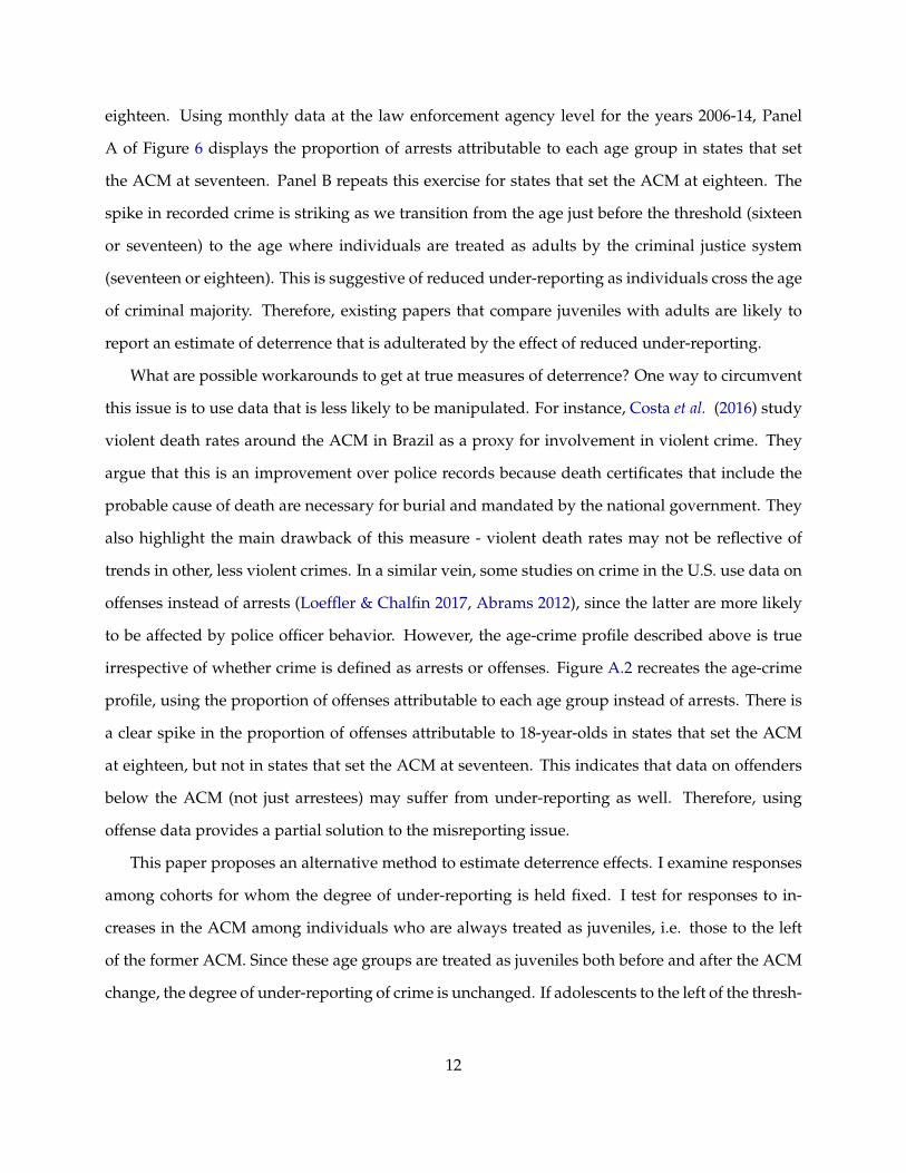
eighteen. Using monthly data at the law enforcement agency level for the years 2006-14, Panel

A of Figure 6 displays the proportion of arrests attributable to each age group in states that set

the ACM at seventeen. Panel B repeats this exercise for states that set the ACM at eighteen. The

spike in recorded crime is striking as we transition from the age just before the threshold (sixteen

or seventeen) to the age where individuals are treated as adults by the criminal justice system

(seventeen or eighteen). This is suggestive of reduced under-reporting as individuals cross the age

of criminal majority. Therefore, existing papers that compare juveniles with adults are likely to

report an estimate of deterrence that is adulterated by the effect of reduced under-reporting.

What are possible workarounds to get at true measures of deterrence? One way to circumvent

this issue is to use data that is less likely to be manipulated. For instance, Costa et al. (2016) study

violent death rates around the ACM in Brazil as a proxy for involvement in violent crime. They

argue that this is an improvement over police records because death certificates that include the

probable cause of death are necessary for burial and mandated by the national government. They

also highlight the main drawback of this measure - violent death rates may not be reflective of

trends in other, less violent crimes. In a similar vein, some studies on crime in the U.S. use data on

offenses instead of arrests (Loeffler & Chalfin 2017, Abrams 2012), since the latter are more likely

to be affected by police officer behavior. However, the age-crime profile described above is true

irrespective of whether crime is defined as arrests or offenses. Figure A.2 recreates the age-crime

profile, using the proportion of offenses attributable to each age group instead of arrests. There is

a clear spike in the proportion of offenses attributable to 18-year-olds in states that set the ACM

at eighteen, but not in states that set the ACM at seventeen. This indicates that data on offenders

below the ACM (not just arrestees) may suffer from under-reporting as well. Therefore, using

offense data provides a partial solution to the misreporting issue.

This paper proposes an alternative method to estimate deterrence effects. I examine responses

among cohorts for whom the degree of under-reporting is held fixed. I test for responses to in-

creases in the ACM among individuals who are always treated as juveniles, i.e. those to the left

of the former ACM. Since these age groups are treated as juveniles both before and after the ACM

change, the degree of under-reporting of crime is unchanged. If adolescents to the left of the thresh-

12

old increase criminal activity when the ACM is moved further away from them, reported crime

should increase. Furthermore, this response is a deterrence effect, since juveniles are responding

to the expectation of lower sanctions in the future by increasing offending in the current period.

Street Gangs in the U.S. & Gang-Related Crime

This section uses criminological studies and national gang surveys to characterize youthful in-

volvement in street gangs in the United States. Crimes most likely to be related to street gangs are

the focus of the empirical analysis. The objective of this separation exercise is not to suggest that

other crimes cannot react to the ACM change - in fact, they may react strongly if there is enough

overlap between "gang" and "non-gang" crimes. Instead, the aim is to test whether the types of

crime that fit the framework of criminal capital accumulation actually do respond to the ACM

change.

Gangs18 are a growing problem in the United States. Following a steady decline until the early

2000s, annual estimates of gang prevalence and gang-related violent, property and drug crimes

have steadily increased (National Gang Center 2012, Egley et al. 2010).19 Street gangs are central

to the discussion of juvenile crime for two reasons. One, a large proportion of gang members are

juveniles - the 2011 National Youth Gang Survey estimates that over a third of all gang members

are under the age of eighteen, and Pyrooz & Sweeten (2015) estimate that there are over a million

juvenile gang members in the U.S. today. Two, gang members contribute disproportionately to

overall crime, particularly to violent adolescent crime. For instance, Thornberry (1998) and Fagan

(1990) documented that while gang membership ranged from 14 to 30 per cent across six cities -

Rochester, Seattle, Denver, San Diego, Los Angeles and Chicago - gang members contributed to at

least sixty percent of drug dealing offenses and sixty percent of general delinquency and serious

violence.20

Which crimes are most commonly associated with street gangs in the U.S.? Past work has

18The FBI National Crime Information Center defines a gang as three or more persons that associate for the purposeof criminal or illegal activity.

19Also see https://www.usnews.com/news/articles/2015/03/06/gang-violence-is-on-the-rise-even-as-overall-violence-declines

20Crime definitions varied by city. Recent research has also shown that this heightened delinquency cannot simply beattributed to individual selection effects (Barnes et al. 2010), and is likely to be associated with gang affiliation itself.

13

shown that gang members are not crime specialists (National Gang Center 2012, Thornberry 1998,

Fagan 1990, Klein & L. Maxson 2010). This finding is confirmed by the FBI’s 2015 National Gang

Report, which collected information from law enforcement agencies about the degree of street gang

involvement in various criminal activities.21 I define gang-related offenses as those for which street

gang involvement is reported as moderate or high in this report. These include eleven UCR offense

categories - homicide, robbery, assault, burglary, theft (including motor vehicle theft), stolen prop-

erty offenses, forgery and fraud, vandalism, weapon law violations and drug offenses.22

Street gangs in the U.S. provide an environment in which juveniles can accumulate criminal

experience and access additional criminal opportunities, lending support to the assumptions of

the theoretical framework. Additionally, previous involvement with law enforcement makes gang

members more likely to be informed about changes in the ACM. These two features indicate that

gang-related crime should react in line with the predictions of the model. Therefore, I use gang-

related offenses to test the main predictions of the model. I also examine responses among offense

categories with at most a low level of street gang involvement - arson, embezzlement, gambling,

offenses against the family and children, driving under the influence and liquor laws, disorderly

conduct (including drunkenness), and suspicion (including vagrancy and loitering).23 The absence

of an increase in "non-gang" crimes is used to rule out the hypothesis that general crime trends are

driving the deterrence results found for "gang-related" crimes.

Data

Local law enforcement agencies in the United States choose to report crime statistics to federal

agencies in one of two ways - the Uniform Crime Reports (UCR) and the National Incident Based

Reporting System (NIBRS). This paper makes use of both of these data sources; the UCR covers

more law enforcement agencies in the U.S., while the NIBRS presents a more detailed picture of

21The survey question asked respondents to indicate whether gang involvement in various criminal activities in theirjurisdiction was High, Moderate, Low, Unknown or None.

22This crime pattern is broadly corroborated by Klein & L. Maxson (2010).23I exclude from the empirical analysis the following offense categories - sex offenses, since the UCR definition of

offenses classified as rape changed in 2013; runaways, a status offense which only applies to juveniles and would beexpected to mechanically increase when 17-year-olds are treated as juveniles; uncategorized crimes, due to the lack ofinterpretability for these results. These three categories account for around 27% of total arrests.

14

crime within the agencies that it covers.

The Uniform Crime Reports have been compiled by the Federal Bureau of Investigation (FBI)

since 1930. UCR data contain monthly data on criminal activity within the agency’s jurisdiction,

with subtotals by arrestee age and sex under each offense category.24 As of 2015, law enforce-

ment agencies representing over ninety per cent of the U.S. population have submitted their crime

data via the UCR. This study uses monthly data at the law enforcement agency level for the six

Northeastern states during 2006-15.

The National Incident Based Reporting System (NIBRS) collects information on each crime

occurrence known to the police, and generates data as a by-product of local, state and federal au-

tomated records management systems. Importantly, offender profiles are generated independent

of arrest using victim and witness statements. This allows us to examine separately whether re-

porting behavior, not just arrest behavior, is influenced by the age of the offender. As of 2012, law

enforcement agencies representing twenty eight per cent of the population have submitted their

crime data via the NIBRS.

To examine how juveniles accumulate criminal experience by offending and associating with

delinquent peers, I use the National Longitudinal Survey of Youth 1997 (NLSY97). The NLSY97

is a nationally representative sample of approximately 9,000 youths who were twelve to sixteen

years old as of December 31, 1996. This dataset includes self-reports on gang membership and

criminal involvement (property, drug, assault and theft offenses) in the preceding twelve months

for each year between 1997 and 2001. I use these responses as representative of the age at which

the respondent spent the majority of the previous twelve months, and create age profiles for gang

membership and criminal involvement, separating states by their ACM.25

3 Theoretical Framework

This section presents a model of criminal behavior in which individuals are aware of the existence

of the ACM and internalize that current criminal activity increases the return to future criminal

24In an incident wherein multiple offenses were committed, only the crime that has the highest rank order in the listof ordered categories will be counted in the monthly totals.

25Pyrooz & Sweeten (2015) create gang membership by age profiles, but do not separate states by their ACM.

15

offending. This framework isolates a deterrence response by identifying cohorts that increase

criminal activity in response to the change in the ACM, and then pinpoints cohorts for which

under-reporting confounds are unlikely to be an issue.

Life-Cycle Model of Crime with an Anticipated Threshold

In Becker (1968)’s seminal framework, individuals undertake criminal activity if the benefits of

crime outweigh the costs. I extend this model to allow individuals to accumulate criminal capital

as they undertake criminal activity over their life course in a continuous time framework.26 In line

with recent work27 criminal capital increases the return to future crime.28 Individuals can only

benefit from criminal capital by committing more crime in the future.

Adolescents are indexed by age t and have preferences that are represented by an intertempo-

rally separable utility function u(ct, kt, st). At each at age, adolescents decide how much criminal

activity ct to undertake, knowing that they will face criminal sanctions st if caught. The return to

criminal activity is an increasing, concave function of criminal capital kt.

u(ct, kt, st) = R(kt).ct � Prob(Caught).st

Rk � 0 Rkk 0

ct � 0

The probability of facing criminal sanctions p(.) is assumed to be an increasing convex function of

criminal activity ct.29

26This is similar to the discrete time framework of Munyo (2015) in which both work- and crime-specific human cap-ital evolve with past choices. Also related are Lee & McCrary (2017), who use a dynamic extension of Becker (1968) andthe static model of time allocation by Grogger (1998) in which individuals allocate time between leisure, formal workand criminal activity. However, the return to crime is assumed to be independent of previous criminal involvement inboth of these studies.

27Pyrooz et al. (2013) and Carvalho & Soares (2016) show that embeddedness and wages in gangs increase withparticipation in gang-related crime. Also see Levitt & Venkatesh (2000) who find that gang members are motivated bythe symbolic value attached to upward mobility in drug gangs, as well as the tournament for future riches.

28This insight is also similar to that of the rational addiction literature, which argues that individual decision makingreflects knowledge of inter-temporal complementarities in consumption. See Becker & Murphy (1988) for a theoreticalexposition.

29This assumption is motivated by the fact that serious offenses are more likely to be reported to the police. Forinstance, the 2010 National Victimization Survey reports that less than 15 per cent of motor vehicle thefts were notreported to the police, while the analogous estimate for all other thefts was over 65 per cent.

16

u(ct, kt, st) = R(kt).ct � p(ct).st

pc � 0 pcc � 0

Criminal activity adds to an individual’s stock of criminal capital, which depreciates at the rate �.

Therefore, the change in criminal capital at each age is current criminal activity ("investment") less

depreciation.

kt = ct � �kt

0 < � < 1

Sanctions s for criminal offenses are a function of age t, and increase sharply as adolescents surpass

the ACM T .

st =

8>>><

>>>:

SJ t < T

SA t � T

0 < SJ < SA

Individuals are forward-looking and maximize lifetime utility. Future flow utility is discounted at

the rate ⇢ 2 (0, 1). The inter-temporal separability of the utility function allows us to write lifetime

utility Ut as the discounted sum of flow utilities ut.

Ut =R1t e�⇢(⌧�t)u(c⌧ , k⌧ , s⌧ )d⌧

At each age t, individuals choose how much crime to undertake ct to maximize lifetime utility,

subject to the criminal capital accumulation equation.

Vt = MaxctR1t e�⇢(⌧�t)u(c⌧ , k⌧ , s⌧ )d⌧

s.t. kt = ct � �kt

To solve this maximization problem, we first set up the current value Hamiltonian. Assume for

now that sanctions st do not vary with t (or that s = SJ = SA). The initial level of criminal capital

k0 is given.30

30k0 determines the return to criminal activity for an individual with no criminal experience, and may be influencedby the criminal experience of one’s peer group or access to criminal opportunities.

17

H(ct, kt) = u(ct, kt,SJ ) + �t(ct � �kt)

ct, the control variable, can be chosen freely; kt is the state variable, since its value is determined by

past decisions; �t, the costate variable, is the shadow value of the state variable kt. The Maximum

Principle generates three conditions characterizing the optimum path for (ct, kt,�t):

Hc = 0 =) R(kt)� pc(ct)SJ + �t = 0 (2a)

Hk = ⇢�t � �t =) Rk(kt)ct � ��t = ⇢�t � �t (2b)

limt!1e�⇢t�tkt 0 (2c)

Equation (2a) pins down the optimal level of criminal activity at each age, and can be rewritten as

pc(ct)SJ = R(kt) + �t

Individuals choose ct to equate the marginal cost of crime pc(ct)SJ with the marginal benefits of

crime. Benefits from crime consist of the current return R(kt) plus the value of an additional unit

of criminal capital in the future �t.

Equation (2b) can be integrated to obtain the following expression

�t =R1t e�(⇢+�)(⌧�t)Rk(k⌧ )c⌧d⌧

�t represents the shadow value of criminal capital kt, and is equal to the present discounted value

of future marginal returns to criminal capital. This implies that expectations about future deci-

sions will influence the valuation of criminal capital in the current period. For instance, if criminal

activity is expected to decrease in the future, �t will decrease even if returns to ct are high in the

current period t.

Equation (2c) specifies that the value of criminal capital cannot accumulate at a rate faster than

18

the discount rate on the optimal path. This ensures that optimizing individuals do not accumulate

criminal capital that they do not intend to utilize.

Dynamics Under Fixed Sanctions

For simplicity, I fix R(kt) = k↵t , ↵ 2 (0, 1) and p(ct) = c2t . Re-arranging the capital accumulation

equation and first order conditions, dynamics in the model can be summarized by:

kt = ct � �kt = 12SJ

(k↵t + �t)� �kt

�t = (⇢+ �)�t � ↵ctk↵�1t = (⇢+ �� ↵

2SJk↵�1t )�t � ↵

2SJk2↵�1t

Figure 1 displays the kt = 0 and �t = 0 loci graphically.31 The arrows show how kt and �t must

behave in order to satisfy conditions (2a) and (2b), given their initial values. The kt = 0 and �t = 0

loci intersect at the steady state level of capital of criminal capital - optimizing individuals will not

wish to increase or decrease their stock of criminal capital once they’ve accumulated k = kSSJ . In

the Appendix, I show that that the steady state level of k is given by

kSSJ = [ 12SJ�

{ ↵(⇢+�) + 1}] 1

1�↵

The steady state value of criminal capital decreases in criminal sanctions SJ , depreciation rate �

and the rate at which future utility is discounted ⇢; kSSJ increases with the returns to additional

criminal capital ↵.

This system of differential equations exhibits saddle path stability for a wide range of param-

eter values, described in detail in the Appendix.32 Recall that the initial value of capital k0 is

assumed to be given, while the shadow value of capital �0 is free to adjust. Saddle path stability

means that there is a unique value of �0 (on the saddle path, shown as the dashed line) such that

kt and �t converge to the steady state. If �0 starts below the saddle path, the individual eventually

crosses into the region where both kt and �t are falling indefinitely. If �0 starts above the saddle

path, the individual eventually crosses into the region where both kt and �t are rising indefinitely.

31This figure is drawn using the following parameter values: ↵ = 0.4, � = 0.3, ⇢ = .05, s = 10.32For instance, 0 < ↵ 0.5 is a sufficient condition for saddle path stability.

19

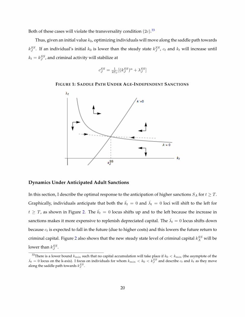
Both of these cases will violate the transversality condition (2c).33

Thus, given an initial value k0, optimizing individuals will move along the saddle path towards

kSSJ . If an individual’s initial k0 is lower than the steady state kSSJ , ct and kt will increase until

kt = kSSJ , and criminal activity will stabilize at

cSSJ = 12SJ

[(kSSJ )↵ + �SSJ ]

FIGURE 1: SADDLE PATH UNDER AGE-INDEPENDENT SANCTIONS

Dynamics Under Anticipated Adult Sanctions

In this section, I describe the optimal response to the anticipation of higher sanctions SA for t � T .

Graphically, individuals anticipate that both the kt = 0 and �t = 0 loci will shift to the left for

t � T , as shown in Figure 2. The kt = 0 locus shifts up and to the left because the increase in

sanctions makes it more expensive to replenish depreciated capital. The �t = 0 locus shifts down

because ct is expected to fall in the future (due to higher costs) and this lowers the future return to

criminal capital. Figure 2 also shows that the new steady state level of criminal capital kSSA will be

lower than kSSJ .

33There is a lower bound kmin

such that no capital accumulation will take place if k0 < kmin

(the asymptote of the�t

= 0 locus on the k-axis). I focus on individuals for whom kmin

< k0 < kSS

J

and describe ct

and kt

as they movealong the saddle path towards kSS

J

.

20

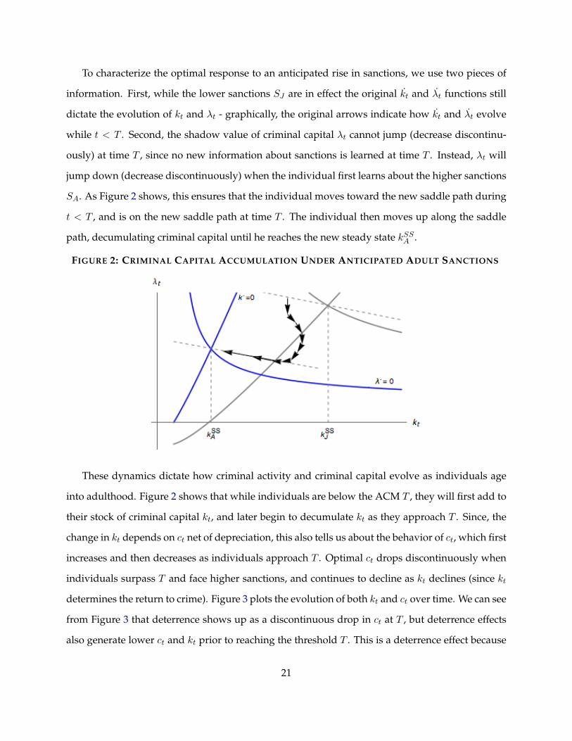
To characterize the optimal response to an anticipated rise in sanctions, we use two pieces of

information. First, while the lower sanctions SJ are in effect the original kt and �t functions still

dictate the evolution of kt and �t - graphically, the original arrows indicate how kt and �t evolve

while t < T . Second, the shadow value of criminal capital �t cannot jump (decrease discontinu-

ously) at time T , since no new information about sanctions is learned at time T . Instead, �t will

jump down (decrease discontinuously) when the individual first learns about the higher sanctions

SA. As Figure 2 shows, this ensures that the individual moves toward the new saddle path during

t < T , and is on the new saddle path at time T . The individual then moves up along the saddle

path, decumulating criminal capital until he reaches the new steady state kSSA .

FIGURE 2: CRIMINAL CAPITAL ACCUMULATION UNDER ANTICIPATED ADULT SANCTIONS

These dynamics dictate how criminal activity and criminal capital evolve as individuals age

into adulthood. Figure 2 shows that while individuals are below the ACM T , they will first add to

their stock of criminal capital kt, and later begin to decumulate kt as they approach T . Since, the

change in kt depends on ct net of depreciation, this also tells us about the behavior of ct, which first

increases and then decreases as individuals approach T . Optimal ct drops discontinuously when

individuals surpass T and face higher sanctions, and continues to decline as kt declines (since kt

determines the return to crime). Figure 3 plots the evolution of both kt and ct over time. We can see

from Figure 3 that deterrence shows up as a discontinuous drop in ct at T , but deterrence effects

also generate lower ct and kt prior to reaching the threshold T . This is a deterrence effect because

21

in the absence of adult sanctions, ct and kt would have converged towards their original steady

state levels (represented by the dotted grey lines).34

FIGURE 3: ct AND kt UNDER ANTICIPATED ADULT SANCTIONS

Notes: The dashed line marks the optimal paths for ct

and kt

if sanctions stay fixed at SJ

.

Comparative Statics

Entry Decisions

In the above analysis, each individual’s non-crime utility was normalized to zero. It is straight-

forward to show that if the outside option (or alternative to crime) improves, individuals are less

likely to commit crime in the first place.

Entry decisions are also influenced by the initial stock of criminal capital k0, since it determines

the payoff to crime. Individuals who begin wth a high initial stock of criminal capital, perhaps

because they live in areas where returns to crime are high or their peers are criminally active, are

predicted to be more likely to begin offending, leading to a self-perpetuating cycle of increases in

criminal capital and criminal activity. This prediction is consistent with papers that document very

large geographic heterogeneity in criminal offending, including the existence of crime "hot spots"

(Eriksson et al. 2016, O’ Flaherty & Sethi 2014).

34It is not necessary that (kt

,�t

) cross the original kt

= 0 locus, as shown in Appendix Figures A.3 and A.4. Here,kt

and ct

continue to increase until age T , but are lower than they would be in the absence of adult sanctions. Thepredicted response to an increase in the age of criminal majority T remains the same.

22

Myopic Juveniles

Individuals who are not forward looking (⇢ = 1) will maximize flow utility, and not lifetime

utility. This means that they will not internalize the future benefits of criminal capital while making

decisions. The maximization problem is a static one (as in Becker 1968), in which individuals

commit crime if the current benefits outweigh the current costs. Therefore, the amount of criminal

activity that individuals at age t with criminal capital kt will undertake is given by

ct =k↵t2st

In this case, criminal activity should decrease sharply when sanctions st rise as individuals cross

the ACM, and the only tests for deterrence are to compare juveniles on either side of the threshold,

or examine the behavior of the "newly juvenile group" (the group between T and T 0) when the age

threshold is moved from T to T 0. However, past estimates of the change in criminal activity at the

threshold have either been small (Lee & McCrary 2017) or negligible (Hjalmarsson 2009, Costa et al.

2016). This paper argues that these small effects could be due to mismeasurement of official data,

but also because individuals who are deterred by the threat of adult sanctions may exit criminal

lifestyles even before reaching the threshold.

Forward-Looking Adolescents

This section focuses on the subset of adolescents who are both informed of the age threshold, and

forward looking (⇢ < 1). The model predicts that that when the ACM is raised from T to T 0, three

groups should increase criminal activity - age groups close to but below T , age groups between

T and T 0, and age groups close to and above T 0. These predictions are tested in Section 5 using

recent ACM variation in the Northeastern states.

The first group to benefit from the ACM rise from T to T 0 is individuals below T 0, since each of

them will face lower sanctions (if caught) for an additional year. In response, individuals will begin

to increase criminal activity and accumulate additional criminal capital, as shown in Figures 4 and

5. For instance, a sixteen year old who would have reduced criminal offending and exited his gang

before he turned seventeen (T ), may postpone exit for an additional year when the ACM is shifted

23

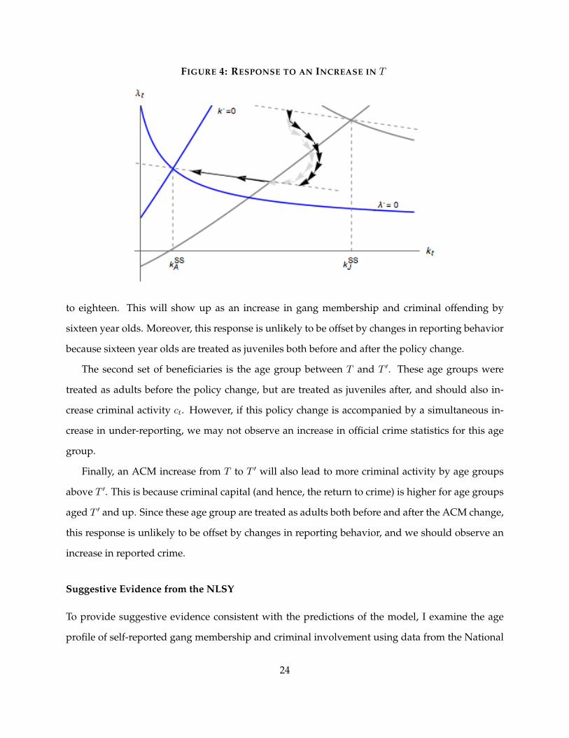
FIGURE 4: RESPONSE TO AN INCREASE IN T

to eighteen. This will show up as an increase in gang membership and criminal offending by

sixteen year olds. Moreover, this response is unlikely to be offset by changes in reporting behavior

because sixteen year olds are treated as juveniles both before and after the policy change.

The second set of beneficiaries is the age group between T and T 0. These age groups were

treated as adults before the policy change, but are treated as juveniles after, and should also in-

crease criminal activity ct. However, if this policy change is accompanied by a simultaneous in-

crease in under-reporting, we may not observe an increase in official crime statistics for this age

group.

Finally, an ACM increase from T to T 0 will also lead to more criminal activity by age groups

above T 0. This is because criminal capital (and hence, the return to crime) is higher for age groups

aged T 0 and up. Since these age group are treated as adults both before and after the ACM change,

this response is unlikely to be offset by changes in reporting behavior, and we should observe an

increase in reported crime.

Suggestive Evidence from the NLSY

To provide suggestive evidence consistent with the predictions of the model, I examine the age

profile of self-reported gang membership and criminal involvement using data from the National

24

FIGURE 5: CRIME RESPONSE TO AN INCREASE IN T

Longitudinal Survey of Youth. A panel of 8,984 adolescents were asked about gang membership

and criminal involvement (property, drug, assault and theft offenses) in the twelve months preced-

ing the interview. I use these self-reports to examine whether (1) gang membership and criminal

involvement decreases as individuals approach the ACM and (2) whether this decrease begins

earlier in states that set the ACM at seventeen instead of eighteen.

The first panel of Figure 7 displays the relationship between gang membership and age for

adolescents in all U.S. states that set their ACM at 17 or 18 (as in Pyrooz & Sweeten 2015). Gang

membership peaks at ages fifteen and sixteen and declines at ages seventeen and above. The

second panel of Figure 7 also shows the age profile of male gang membership, but separates states

by their ACM. Here, we find evidence suggestive of earlier exit in states that set the ACM at

seventeen, consistent with the predictions of the model. In particular, gang membership peaks

earlier (at fifteen) and begins its decline earlier (at sixteen) in states that set the ACM at seventeen.

In states that set the ACM at eighteen, gang membership peaks at sixteen, and then declines at

ages seventeen and eighteen. Figure A.5 shows that including female respondents leads to similar

patterns of gang membership by age.

Figure 8 examines whether the relationship between criminal involvement and age varies with

the ACM. The first panel depicts this relationship for adolescents in all U.S. states that set their

ACM at 17 or 18 - we see a clear upward trend until sixteen, and a sharp decline at seventeen.

25

The second panel also displays the age-crime relationship but separates states by their ACM. Two

points are worth noting about this graph. One, criminal involvement in higher for all age groups

under eighteen. Two, the decline in criminal involvement begins earlier (at age sixteen) in states

that set the ACM at seventeen, and appears later, at age seventeen, in states that set the ACM at

eighteen. Both patterns are consistent with the predictions of the model. Figure A.5 repeats this

analysis for the sample including female respondents and shows that patterns of criminal involve-

ment by age are similar. In Section 5, I show that this pattern of higher criminal involvement for

all age groups under eighteen is at least partly driven by the higher age of criminal majority.

4 Empirical Strategy

This section describes the difference-in-difference-in-difference (DDD) framework used to identify

the impact of an ACM increase on adolescent offending. I restrict attention to the six neighboring

Northeastern states that have introduced legislation to raise the ACM since 2006. These states

can be divided into two groups - those in which the legislation was successful and the ACM was

modified (Connecticut, Massachusetts, New Hampshire and Rhode Island) and those in which the

ACM was left unchanged (New York, Vermont). The DDD technique compares those who were

affected by the ACM increase (adolescents) with individuals that were not (older adults) in the two

groups of states, before and after the ACM change.

Central Specification

I estimate the following DDD specification with age, state and year fixed effects, as well as age-

state, state-year and age-year interactions:

Calsmy = �0 + �1AFFECTa ⇤TREATs ⇤POSTsmy + �a + �s + �y + �as + �sy + �ay + �my + "alsmy

Calsmy is a measure of the crime rate among age group a in location l in state s during month m of

year y. As a measure of the crime rate, I use the number of arrestees aged a per 100,000 residents

in location l. State and age fixed effects (�a and �s) account for permanent differences across states

26

and age groups. Year fixed effects �y account for national crime trends. I also include month fixed

effects �my to control more flexibly for national crime trends.

This specification includes a full set of state-year interactions �sy which control flexibly for

factors that may be changing at the state-year level that could affect my outcomes of interest.

Age-state interactions �as allow for permanent differences across age groups in different states.

Age-year interactions �ay control flexibly for national trends that may affect one age group more

than another. Since treatment varies at the age level within each state, standard errors "alsmy are

clustered at the age-state level.

AFFECTa is an indicator variable that equals one for age groups 21 and under. TREATs is

an indicator variable that equals one if state s raised its ACM during the study period 2006-15.35

POSTsmy is an indicator variable that equals one if the ACM change in state s is in effect in month

m of year y. The coefficient of interest is �1, which is the DDD estimate of the effect of an ACM

increase on adolescent offending.

Event Study Specification

In order to examine the year-by-year impact of the ACM change, I use the following event study

specification:

Calsmy = Âi��n �iAFFECTa ⇤TREATs ⇤POST ismy + �a+ �s+ �y + �as+ �sy + �ay + �my + "alsmy

Calsmy is a measure of the crime rate among age group a as described above. POST ismy are indi-

cator variables that equal 1 if the ACM was increased in state s exactly i years before period t. For

instance, Connecticut raised its ACM from 17 to 18 on July 1, 2012, so the POST 1 dummy equals

1 for Connecticut during July 2012 - June 2013, the POST 2 dummy equals 1 for Connecticut for

the period July 2013 - June 2014, and so on. Also notice that i may take on negative values, which

allows us to test for differences prior to the policy’s implementation. Regressions continue to con-

trol for age, state and year fixed effects, as well as age-state, state-year and age-year interactions.

35Rhode Island lowered its ACM from 18 to 17 for the period July - November 2007. TREATs=Rhode Island

takes onthe value -1, which ensures that �1 can be interpreted as the impact of an increase in the ACM.

27

Standard errors are clustered at the age-state level to adjust for serial correlation.36

Crime Indices

As mentioned above, I use the number of arrests per 100,000 residents as a measure of the local

crime rate. However, this outcome variable may be comprised mostly of a handful of frequently

occurring offenses such as theft, and not account adequately for serious but less frequent offenses

such as homicide. To overcome this drawback of the raw arrest rate, I create a crime index based

on offense-specific arrest rates as an alternative measure of local crime. Each index is defined as the

equally weighted average of the z-scores of its components (offense-specific arrest rates). Z-scores

are calculated by subtracting the control group mean and dividing by the control group standard

deviation.37

I construct two crime indices. The first index uses arrest rates for offenses categories that have

a medium or high level of street gang involvement as per the FBI’s 2015 National Gang Report.

These include drug, homicide, robbery, assault, burglary, theft (including motor vehicle theft and

stolen property offenses), forgery and fraud, vandalism and weapon law violations. The second

index uses arrest rates for offense categories that have at most a low level of street gang involve-

ment. These include arson, embezzlement, gambling, offenses against the family and children,

driving under the influence and liquor laws, disorderly conduct (including drunkenness), and

suspicion (including vagrancy and loitering). The objective of this separation exercise is not to

suggest that other crimes cannot react to the ACM change - in fact, they may react strongly if there

is enough overlap between "gang" and "non-gang" crimes. Instead, the aim is to test whether the

types of crime that benefit from the accumulation of criminal capital actually do respond to the

ACM change.

36Since Rhode Island only changed its ACM for four months before reversing it back, I include it in the control groupfor the event study regressions.

37Results are robust to using scores based on inverse variance weighting and are available on request.

28

5 Results

In this section, I show that postponing the threat of adult sanctions leads to an increase in juvenile

offending. When the age of criminal majority is increased from 17 to 18, individuals aged seven-

teen and under increase criminal activity. This increase is driven by offenses related to street gangs,

including drug, homicide, robbery, theft, vandalism and burglary offenses. A back-of-the-envelope

calculation shows that for every seventeen year old that was transferred to juvenile facilities as a

result of the ACM increase, jurisdictions bore social costs of $65,000 due to the increase in juvenile

offending.

The setting for the empirical tests is a group of neighboring Northeastern States, namely Con-

necticut, Massachusetts, New Hampshire, New York, Rhode Island and Vermont. Each of these

states has experimented with raising the ACM since 2005, lending credibility to the assumption

that the actual timing of ACM changes within these states was exogenous, or unrelated to local

crime trends. These results are based on a balanced panel of agencies that submit data via the

Uniform Crime Reports for the period 2006-15.

5.1 Juvenile Crime

I first test whether increasing the ACM from 17 to 18 led to an increase in overall arrest rates for

13-17-year-olds. These results are presented in the first column of Table 1, which shows that the

monthly arrest rate increased by around 0.31, or 6 per cent of the mean, for each age group in the

range 13-17.

The second column reports analogous estimates for arrest rates for offenses with a medium or

high level of street gang involvement, based off of the FBI’s 2015 National Gang Report. Here we

see that the previously documented increase is entirely driven by offenses associated with street

gangs, for which arrest rates increase by 0.34, or 7 per cent of the mean. Since the above estimate

may be driven by a handful of frequently occurring offenses, I also examine effects on a crime

index based on gang-related offenses (which weights offense categories equally). The lower panel

of Table 1 shows that the gang-related crime index increases, and that this estimate is statistically

significant at the 1 per cent level.

29

The third column reports analogous estimates for offenses with at most a low level of street

gang involvement, such as driving under the influence and liquor law violations. These offense

categories do not respond to the increase in the ACM - the estimated coefficient is small and statis-

tically indistinguishable from zero. Using a crime index based on these offense categories leads to

similar results - the estimated coefficient is negative and statistically indistinguishable from zero.

5.2 Age-Specific Estimates

The previous section presented a broad overview of the average impact of the ACM increase on

juvenile crime. In this section, I present age-specific estimates of the impact of the ACM increase

on both gang-related and other offenses. As predicted by the model, I show that the ACM increase

also leads to an increase in offending by those above the age of eighteen, since these adolescents

are now associated with a higher level of criminal capital, and their return to offending will be

higher than previous cohorts’.

Table 2 displays the estimated impact on arrest rates and crime indices for each age group in

the age range 13-21.38 The first two columns present results for offenses with a medium or high

level of street gang involvement - arrest rates increase for 13-16-year-olds by around 12 per cent

of the mean, and for 18-year-olds by around 8 per cent of the mean. The first panel of Figure 9

displays these age-specific estimates graphically. The smaller, statistically insignificant estimate

for 17-year-olds is particularly conspicuous. However, this finding may be driven by the fact that

seventeen year-olds are simultaneously exposed to lower sanctions as well as an increase in under-

reporting. The latter effect appears to offset the effect of lower sanctions, which can be observed

much more clearly for those aged 13-16 and 18.

Next, I use an event study specification to examine the year-by-year impact of the ACM in-

crease on arrests for gang-related offenses in the age group 13-21. The second panel of Figure 9

displays DDD coefficients for five years before and four years after the policy’s implementation.

We see a clear increase in arrest rates starting in the first year of the ACM change. Further, this

effect increases over time.38The Uniform Crime Reports only report collective data for 13 and 14 year old arrestees.

30

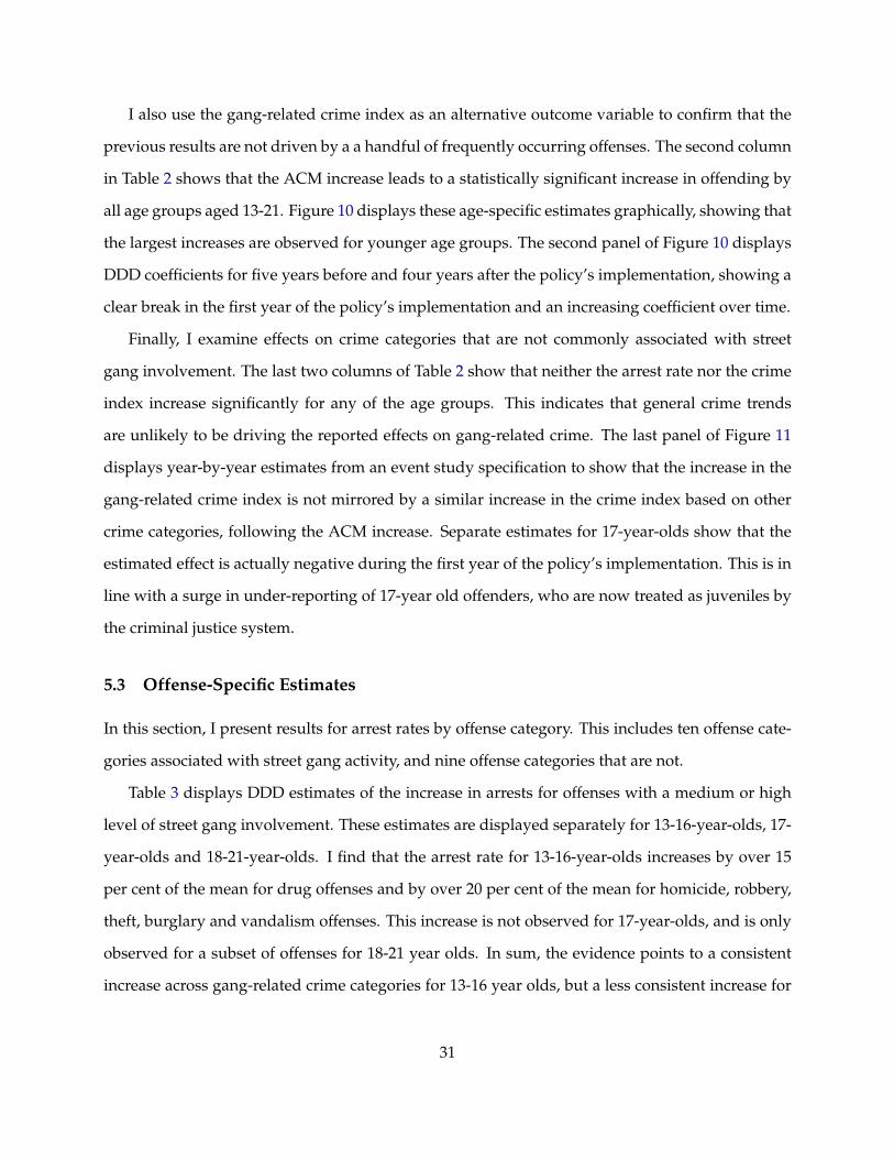
I also use the gang-related crime index as an alternative outcome variable to confirm that the

previous results are not driven by a a handful of frequently occurring offenses. The second column

in Table 2 shows that the ACM increase leads to a statistically significant increase in offending by

all age groups aged 13-21. Figure 10 displays these age-specific estimates graphically, showing that

the largest increases are observed for younger age groups. The second panel of Figure 10 displays

DDD coefficients for five years before and four years after the policy’s implementation, showing a

clear break in the first year of the policy’s implementation and an increasing coefficient over time.

Finally, I examine effects on crime categories that are not commonly associated with street

gang involvement. The last two columns of Table 2 show that neither the arrest rate nor the crime

index increase significantly for any of the age groups. This indicates that general crime trends

are unlikely to be driving the reported effects on gang-related crime. The last panel of Figure 11

displays year-by-year estimates from an event study specification to show that the increase in the

gang-related crime index is not mirrored by a similar increase in the crime index based on other

crime categories, following the ACM increase. Separate estimates for 17-year-olds show that the

estimated effect is actually negative during the first year of the policy’s implementation. This is in

line with a surge in under-reporting of 17-year old offenders, who are now treated as juveniles by

the criminal justice system.

5.3 Offense-Specific Estimates

In this section, I present results for arrest rates by offense category. This includes ten offense cate-

gories associated with street gang activity, and nine offense categories that are not.

Table 3 displays DDD estimates of the increase in arrests for offenses with a medium or high

level of street gang involvement. These estimates are displayed separately for 13-16-year-olds, 17-

year-olds and 18-21-year-olds. I find that the arrest rate for 13-16-year-olds increases by over 15

per cent of the mean for drug offenses and by over 20 per cent of the mean for homicide, robbery,

theft, burglary and vandalism offenses. This increase is not observed for 17-year-olds, and is only

observed for a subset of offenses for 18-21 year olds. In sum, the evidence points to a consistent

increase across gang-related crime categories for 13-16 year olds, but a less consistent increase for

31

other age groups close the ACM.

To show that general crime trends may not explain the effects documented above, I also exam-

ine the effect of the ACM increase on crime categories that are less likely to involve street gangs.

Table 4 displays DDD estimates for nine offense categories, separately for 13-16-year-olds, 17-year-

olds and 18-21-year-olds. There appears to be no consistent response for these offense categories

amongst 13-16 and 17-year-olds, since many of the estimates are negative, and most are statisti-

cally indistinguishable from zero. There is a statistically significant increase in the 18-21-year-old

arrest rate for disorderly conduct and liquor law violations. However, the estimated impact of

the ACM increase on all other offense categories is small (relative to the mean) and statistically

indistinguishable from zero.

5.4 Demographic Heterogeneity

In this section, I examine which gender and race groups are driving the increase in gang-related

juvenile crime. The first panel of Table 5 shows a significant increase in arrest rates for males of

each age except 17, while the second panel shows a less statistically significant pattern for females.

This finding may be due to the low involvement of females in criminal enterprises like gangs -

for instance, the 2011 National Youth Gang Survey reports that the proportion of female gang

members did not exceed 8 per cent over the period 1998-2010.

The UCR data also report the number of arrests of individuals aged seventeen and under by

race. The last panel of Table 5 shows that the deterrence estimates are largely driven by an in-

crease in the arrest rate for White adolescents39 while the response among Black and Asian adoles-

cents is statistically indistinguishable from zero. This is an intriguing finding because the National

Youth Gang Survey reports that in 2011 around 58 per cent of gang members were White/Hispanic

while 35 per cent were Black. However, this pattern is consistent with effective treatment differing

across race groups. If youth of color are disproportionately charged in adult courts, as reported in

Juszkiewicz (2009), raising the ACM may change their incentives less than those of White youth.

In this situation, it would not be surprising to find larger effects for White adolescents and smaller

39Agencies do not separately report arrests for Hispanic arrestees, who can be included in any of the race categories.

32

effects for adolescents belonging to other race groups.

5.5 Robustness Checks

This section shows that the main results are robust to a number of checks such as varying the level

of clustering, using alternative age cohorts as control groups and extending the study sample to all

states in the U.S. The outcomes of interest are the 13-17-year-old arrest rate and crime index based

on gang-related offenses.

Clustering at the Juvenile-State Level

Clustering standard errors at the age-state level allows for serial correlation within each age group,

but not across juvenile age groups within states. I relax this assumption by clustering at the

juvenile-state level, which allows errors to be serially correlated across all juveniles within a given

state, and across all adults within a given state.

Table A.3 shows that clustering standard errors at the juvenile-state level does not materially

change the main results. The first column shows that while the confidence interval is wider, the

estimated increase in the arrest rate remain statistically significant at the 5 per cent level. Table A.4

reports analogous results for the juvenile gang crime index. Once again, the confidence interval

widens, but the estimated increase remains significant at the 5 per cent level.

Alternative Age Groups as Controls

The previous analysis defines individuals aged 22 and above as control groups. The second and

third columns of Table A.3 shows that the estimated increase in juvenile arrests is not driven by

this choice, and is robust to redefining the control group to include only younger or older age

groups. Table A.4 reports analogous results for the juvenile gang crime index. Both sets of results

are robust to clustering at the juvenile-state level.

33

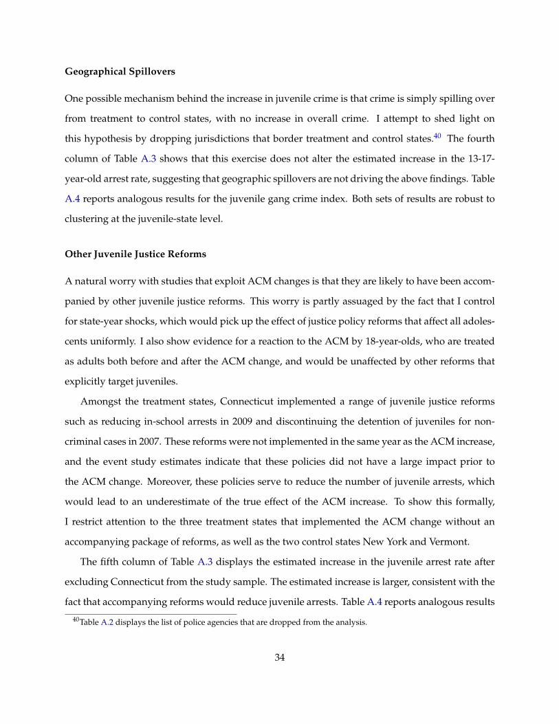
Geographical Spillovers

One possible mechanism behind the increase in juvenile crime is that crime is simply spilling over

from treatment to control states, with no increase in overall crime. I attempt to shed light on

this hypothesis by dropping jurisdictions that border treatment and control states.40 The fourth

column of Table A.3 shows that this exercise does not alter the estimated increase in the 13-17-

year-old arrest rate, suggesting that geographic spillovers are not driving the above findings. Table

A.4 reports analogous results for the juvenile gang crime index. Both sets of results are robust to

clustering at the juvenile-state level.

Other Juvenile Justice Reforms

A natural worry with studies that exploit ACM changes is that they are likely to have been accom-

panied by other juvenile justice reforms. This worry is partly assuaged by the fact that I control

for state-year shocks, which would pick up the effect of justice policy reforms that affect all adoles-

cents uniformly. I also show evidence for a reaction to the ACM by 18-year-olds, who are treated

as adults both before and after the ACM change, and would be unaffected by other reforms that

explicitly target juveniles.

Amongst the treatment states, Connecticut implemented a range of juvenile justice reforms

such as reducing in-school arrests in 2009 and discontinuing the detention of juveniles for non-

criminal cases in 2007. These reforms were not implemented in the same year as the ACM increase,

and the event study estimates indicate that these policies did not have a large impact prior to

the ACM change. Moreover, these policies serve to reduce the number of juvenile arrests, which

would lead to an underestimate of the true effect of the ACM increase. To show this formally,

I restrict attention to the three treatment states that implemented the ACM change without an

accompanying package of reforms, as well as the two control states New York and Vermont.

The fifth column of Table A.3 displays the estimated increase in the juvenile arrest rate after

excluding Connecticut from the study sample. The estimated increase is larger, consistent with the

fact that accompanying reforms would reduce juvenile arrests. Table A.4 reports analogous results

40Table A.2 displays the list of police agencies that are dropped from the analysis.

34

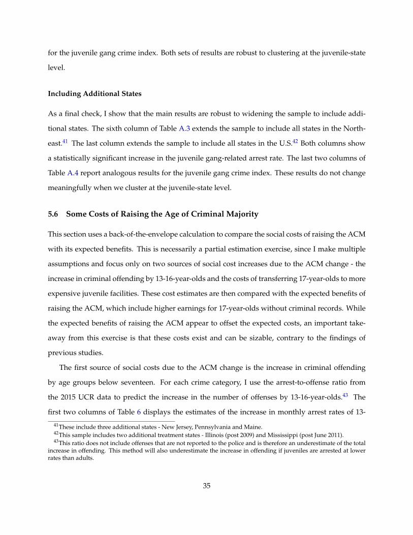
for the juvenile gang crime index. Both sets of results are robust to clustering at the juvenile-state

level.

Including Additional States

As a final check, I show that the main results are robust to widening the sample to include addi-

tional states. The sixth column of Table A.3 extends the sample to include all states in the North-

east.41 The last column extends the sample to include all states in the U.S.42 Both columns show

a statistically significant increase in the juvenile gang-related arrest rate. The last two columns of

Table A.4 report analogous results for the juvenile gang crime index. These results do not change

meaningfully when we cluster at the juvenile-state level.

5.6 Some Costs of Raising the Age of Criminal Majority

This section uses a back-of-the-envelope calculation to compare the social costs of raising the ACM

with its expected benefits. This is necessarily a partial estimation exercise, since I make multiple

assumptions and focus only on two sources of social cost increases due to the ACM change - the

increase in criminal offending by 13-16-year-olds and the costs of transferring 17-year-olds to more

expensive juvenile facilities. These cost estimates are then compared with the expected benefits of

raising the ACM, which include higher earnings for 17-year-olds without criminal records. While

the expected benefits of raising the ACM appear to offset the expected costs, an important take-

away from this exercise is that these costs exist and can be sizable, contrary to the findings of

previous studies.

The first source of social costs due to the ACM change is the increase in criminal offending

by age groups below seventeen. For each crime category, I use the arrest-to-offense ratio from

the 2015 UCR data to predict the increase in the number of offenses by 13-16-year-olds.43 The

first two columns of Table 6 displays the estimates of the increase in monthly arrest rates of 13-

41These include three additional states - New Jersey, Pennsylvania and Maine.42This sample includes two additional treatment states - Illinois (post 2009) and Mississippi (post June 2011).43This ratio does not include offenses that are not reported to the police and is therefore an underestimate of the total

increase in offending. This method will also underestimate the increase in offending if juveniles are arrested at lowerrates than adults.

35

16-year-olds for homicide, assault, robbery, larceny, motor vehicle theft, stolen property, burglary,

vandalism, fraud, forgery and drug offenses following the ACM increase as well as the arrest-

to-offense ratio for each of these crimes. The third column displays McCollister et al. (2010)’s

estimates of societal costs by offense type, which include costs imposed directly on victims and

indirectly on the criminal justice system in the form of legal, police and corrections costs.44 The

fourth column displays the annual increase in costs (including incarceration45) by offense type

due to the uptick in offending, evaluated at the average treatment agency population of 27,200.

Overall, the crime increase among 13-16-year-olds led to an increase of $265,000 in societal costs,

two thirds of which is accounted for by homicide offenses.

The second source of social costs is the transfer of 17-year-olds to juvenile facilities. Juvenile in-

carceration costs in the treatment states average $544 per day (Justice Policy Institute 2014), while

the equivalent estimate for adult incarceration is $198 (Vera Institute of Justice 2017).46 My esti-

mate of the number of such transfers is based on the Office of Juvenile Justice and Delinquency

Prevention’s data on offense-specific probation and incarceration rates for 17-year-olds, displayed

in Table 7.47 The sixth column displays completed sentence lengths specific to each offense cate-

gory (person, property, drug and public order) also reported by the OJJDP. The increase in costs

due to the transfer of 17-year-olds from adult to juvenile facilities is just under $75,000.48

44McCollister et al. (2010) employ cost-of-illness and jury compensation methods to estimate both the tangible andintangible costs of crime. I use their estimates for three reasons - first, they provide the most recent set of estimates;second, they provide cost estimates for more offense categories than Donohue III (2009); third, their estimates for theoverlapping set of offenses are broadly similar to those of other studies like Donohue III (2009) and Cohen et al. (2004).I exclude McCollister et al. (2010)’s estimates of offenders’ productivity losses while incarcerated, since individualsbelow seventeen are unlikely to be a part of the formal labor force. I also supplement these estimated with Mueller-Smith (2016)’s social cost of drug offenses estimate of $2,544. I exclude simple assault and weapon law violations dueto the lack of social cost estimates for these offenses.

45This is likely to be an underestimate, since juvenile incarceration costs over twice as much as adult incarceration. Ialso do not account for the fact that 13-16-year-old offenders who are incarcerated may be more likely to recidivate inthe future.

46Since New Hampshire is not included in the Vera Institute of Justice 2017 report, I use the Vera Institute of Justice2012 estimates assuming that its costs grew at the same rate as Connecticut and Rhode Island, who provided informationin both surveys. Estimates are in 2015 USD.

47Here, I make three assumptions. One, the proportion of 17-year-olds adjudicated delinquent that receive placementsentences (instead of probation sentences) does not change after the increase in the ACM. Two, the cost of probation fora 17-year-old does not change when the ACM is raised to eighteen. Third, the completed duration of incarceration doesnot depend on the ACM, an assumption supported by the findings of Fritsch et al. (1996) and Fagan (Jan/Apr. 1996.).

48If the marginal incarceration cost is around half of the average cost in both juvenile and adult facilities (as found byOwens (2009) in Maryland) the cost increase will be around $37,500.

36

What are the benefits of raising the ACM? Proponents of raising the ACM argue that juvenile

justice policies reduce recidivism. However, recent studies show that incarceration in juvenile fa-

cilities has a large impact on recidivism (Aizer & Doyle 2015) and that adult incarceration may

actually lower recidivism for marginal offenders (Loeffler & Grunwald 2015a). Therefore, I do not

focus on lower recidivism as the primary benefit of raising the age; instead, I estimate the number

of 17-year-olds who will be diverted away from adult prisons and will not receive criminal records.

This estimate is displayed by offense type in the fourth column of Table 7, which sums up to a total

of 5.35 17-year-olds.

The question for policymakers is whether a cost increase of $65,000 per 17-year-old is exceeded

by the potential benefits. There are three reasons why it might - one, the expungement of criminal

records has been shown to increase college completion rates (Litwok 2014), boost employment and

average annual real earnings by around $6,000 (Chapin et al. 2014, Selbin et al. 2017) and reduce

government dependence and increase tax revenues by around $2,200 (Chapin et al. 2014); two, the

transfer to juvenile facilities may lower the risk of assault faced by the average juvenile convict -

McCollister et al. (2010) estimate victim costs alone of over $200,000 for sexual assault and $100,000

for aggravated assault;49 three, if more 17-year-olds receive probation instead of incarceration sen-

tences, Aizer & Doyle (2015) and Bayer et al. (2009)’s findings indicate that we may see an increase

in high school completion rates and a decrease in recidivism. Focusing on the increase of $6,000 in

earnings alone indicates that increasing the ACM may have been a move in the right direction.

6 Conclusion

Recent research shows that criminal involvement can persist into long-term offending, as individ-

uals accumulate skills and experience pertinent to the crime sector (Bayer et al. 2009, Pyrooz et al.

2013, Carvalho & Soares 2016, Sviatschi 2017) or lose human capital valued in the non-crime sector

(Hjalmarsson 2008, Aizer & Doyle 2015). However, existing research on the deterrent effects of the

49It is difficult to quantify the change in assault risk faced by adolescents across different types of facilities. For in-stance, Beck & Hughes (2004) document that rates of reported sexual assault are six times higher in juvenile correctionalfacilities than in adult facilities across the U.S. This is likely driven by state laws specifying that all sexual acts involvingyouth below certain ages are nonconsensual.

37

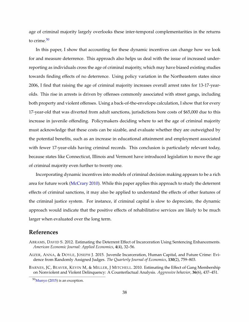
age of criminal majority largely overlooks these inter-temporal complementarities in the returns

to crime.50

In this paper, I show that accounting for these dynamic incentives can change how we look

for and measure deterrence. This approach also helps us deal with the issue of increased under-

reporting as individuals cross the age of criminal majority, which may have biased existing studies

towards finding effects of no deterrence. Using policy variation in the Northeastern states since

2006, I find that raising the age of criminal majority increases overall arrest rates for 13-17-year-

olds. This rise in arrests is driven by offenses commonly associated with street gangs, including

both property and violent offenses. Using a back-of-the-envelope calculation, I show that for every

17-year-old that was diverted from adult sanctions, jurisdictions bore costs of $65,000 due to this

increase in juvenile offending. Policymakers deciding where to set the age of criminal majority

must acknowledge that these costs can be sizable, and evaluate whether they are outweighed by

the potential benefits, such as an increase in educational attainment and employment associated

with fewer 17-year-olds having criminal records. This conclusion is particularly relevant today,

because states like Connecticut, Illinois and Vermont have introduced legislation to move the age

of criminal majority even further to twenty one.

Incorporating dynamic incentives into models of criminal decision making appears to be a rich

area for future work (McCrary 2010). While this paper applies this approach to study the deterrent

effects of criminal sanctions, it may also be applied to understand the effects of other features of

the criminal justice system. For instance, if criminal capital is slow to depreciate, the dynamic

approach would indicate that the positive effects of rehabilitative services are likely to be much

larger when evaluated over the long term.

ReferencesABRAMS, DAVID S. 2012. Estimating the Deterrent Effect of Incarceration Using Sentencing Enhancements.

American Economic Journal: Applied Economics, 4(4), 32–56.

AIZER, ANNA, & DOYLE, JOSEPH J. 2015. Juvenile Incarceration, Human Capital, and Future Crime: Evi-dence from Randomly Assigned Judges. The Quarterly Journal of Economics, 130(2), 759–803.

BARNES, JC, BEAVER, KEVIN M, & MILLER, J MITCHELL. 2010. Estimating the Effect of Gang Membershipon Nonviolent and Violent Delinquency: A Counterfactual Analysis. Aggressive behavior, 36(6), 437–451.

50Munyo (2015) is an exception.

38

BAYER, PATRICK, HJALMARSSON, RANDI, & POZEN, DAVID. 2009. Building Criminal Capital behind Bars:Peer Effects in Juvenile Corrections*. The Quarterly Journal of Economics, 124(1), 105.

BECK, ALLEN J., & HUGHES, TIMOTHY A. 2004. Sexual Violence Reported by Correctional Authorities.Bureau of Justice Statistics Special Report.

BECKER, GARY. 1968. Crime and Punishment: An Economic Approach. Journal of Political Economy, 76.

BECKER, GARY S., & MURPHY, KEVIN M. 1988. A Theory of Rational Addiction. Journal of Political Economy,96(4), 675–700.

BLACK, DONALD J. 1970. Production of crime rates. American sociological review, 733–748.

BLACK, DONALD J. 1971. The Social Organization of Arrest. Stanford Law Review, 23(6), 1087–1111.

BUSHWAY, SHAWN, DEANGELO, GREGORY, & HANSEN, BENJAMIN. 2013. Deterability by age. InternationalReview of Law and Economics, 36, 70 – 81.

CARVALHO, LEANDRO S., & SOARES, RODRIGO R. 2016. Living on the edge: Youth entry, career and exit indrug-selling gangs. Journal of Economic Behavior Organization, 121, 77 – 98.

CHALFIN, AARON, & MCCRARY, JUSTIN. 2014. Criminal Deterrence: A Review of the Literature. J Econ Lit.

CHAPIN, MEYLI, ELHANAN, ALON, RILLERA, MATTHEW, SOLOMON, AUDREY K., & WOODS, TYLER L.2014. A Cost-Benefit Analysis of Criminal Record Expungement in Santa Clara County. UndergraduatePublic Policy Senior Practicum Stanford University, March.

COHEN, MA, RT, RUST, & STEEN S, TIDD ST. 2004. Willingness-to-Pay for Crime Control Programs. Crim-inology, 42, 89–109.

COSTA, FRANCISCO, DE FARIA, JOÃO S, IACHAN, FELIPE, & CABALLERO, BÁRBARA. 2016. Homicidesand the Age of Criminal Responsibility in Brazil: A Density Discontinuity Approach. Available at SSRN:https://ssrn.com/abstract=2670382 or http://dx.doi.org/10.2139/ssrn.2670382.

DAMM, ANNA PIIL, LARSEN, BRITT ØSTERGAARD, NIELSEN, HELENA SKYT, & SIMONSEN, MARIANNE.2017. Lowering the minimum age of criminal responsibility: Consequences for juvenile crime and edu-cation. In: Working Paper.

DONOHUE III, J. 2009. Assessing the relative benefits of incarceration: Overall changes and the benefits onthe margin. In: RAPHAEL, S., & STOLL, M. (eds), Do Prisons Make Us Safer? Russell Sage Foundation.

DRAGO, FRANCESCO, GALBIATI, ROBERTO, & VERTOVA, PIETRO. 2009. The Deterrent Effects of Prison:Evidence from a Natural Experiment. Journal of Political Economy, 117(2), 257–280.

DRAGO, FRANCESCO, GALBIATI, ROBERTO, & VERTOVA, PIETRO. 2011. Prison Conditions and Recidivism.American Law and Economics Review, 13(1), 103–130.

EGLEY, A. JR, HOWELL, J. C., & MOORE, J. P. 2010. Highlights of the 2008 National Youth Gang Survey. In:Department of Justice, Office of Justice Programs. Office of Juvenile Justice and Delinquency Prevention.

ERIKSSON, KARIN HEDEROS, HJALMARSSON, RANDI, LINDQUIST, MATTHEW J., & SANDBERG, ANNA.2016. The importance of family background and neighborhood effects as determinants of crime. Journalof Population Economics, 29(1), 219–262.

FAGAN, J.E. 1990. Social process of delinquency and drug use among urban gangs. Pages 183–219 of: C.R.HUFF. NEWBURY PARK, CA (ed), Gangs in America. Sage Publications.

39

FAGAN, JEFFREY. Jan/Apr. 1996.. The Comparative Advantage of Juvenile vs. Criminal Court Sanctions onRecidivism Among Adolescent Felony Offenders. Law and Policy, Vol. 18 1 and 2.

FRITSCH, ERIC J., CAETI, TORY J., & HEMMENS, CRAIG. 1996. Spare the Needle But Not the Punishment:The Incarceration of Waived Youth in Texas Prisons. Crime and Delinquency, 42, 593.

GLASSNER, BARRY, KSANDER, MARGRET, BERG, BRUCE, & JOHNSON, BRUCE D. 1983. A Note on theDeterrent Effect of Juvenile Vs. Adult Jurisdiction*. Social Problems, 31(2), 219–221.

GREENWOOD, PETER. 1995. Juvenile crime and juvenile justice. In: WILSON, JAMES Q., & PETERSILIA,JOAN (eds), Crime, san francisco: ics edn.

GROGGER, JEFF. 1998. Market Wages and Youth Crime. Journal of Labor Economics, 16(4), 756–791.

HANSEN, BENJAMIN. 2015. Punishment and Deterrence: Evidence from Drunk Driving. American EconomicReview, 105(4), 1581–1617.

HANSEN, BENJAMIN, & WADDELL, GLEN R. 2014. Walk Like a Man: Do Juvenile Offenders Respond toBeing Tried as Adults?”. Unpublished.

HEKMAN, RANDALL J., GOLD, MARTIN, & RUHLAND, DAVID J. 1983. Reducing Crime: It Can Be Done.Juvenile and Family Court Journal, 34(3), 3–7.

HELLAND, ERIC, & TABARROK, ALEXANDER. 2007. Does Three Strikes Deter? A Nonparametric Estima-tion. The Journal of Human Resources, 42(2), 309–330.

HELLER, SARA B., SHAH, ANUJ K., GURYAN, JONATHAN, LUDWIG, JENS, MULLAINATHAN, SENDHIL, &POLLACK, HAROLD A. 2017. Thinking, Fast and Slow? Some Field Experiments to Reduce Crime andDropout in Chicago*. The Quarterly Journal of Economics, 132(1), 1.

HENDREN, NATHANIEL. 2016. Knowledge of Future Job Loss and Implications for Unemployment Insurance.Forthcoming, American Economic Review.

HJALMARSSON, RANDI. 2008. Criminal justice involvement and high school completion. Journal of UrbanEconomics, 63(2), 613 – 630.

HJALMARSSON, RANDI. 2009. Crime and Expected Punishment: Changes in Perceptions at the Age ofCriminal Majority. American Law and Economics Review, 11(1), 209–248.

IMAI, SUSUMU, & KRISHNA, KALA. 2004. Employment, Deterrence, and Crime in a Dynamic Model. Inter-national Economic Review, 45(3), 845–872.

JUSTICE POLICY INSTITUTE, REPORT. 2014. Sticker Shock: Calculating the Full Price Tag for Youth Incarcer-ation.

JUSZKIEWICZ, J. 2009. Youth Crime/Adult Time: Is Justice Served? Building Blocks for Youth Initiative.

KATZ, LAWRENCE, LEVITT, STEVEN, & SHUSTOROVICH, ELLEN. 2003. Prison Conditions, Capital Punish-ment, and Deterrence. American Law and Economics Review, 5(2), 318–343.

KHANNA, GAURAV. 2016. Incentivizing Standards or Standardizing Incentives? Affirmative Action inIndia. Available at SSRN: https://ssrn.com/abstract=2246549.

KLEIN, MALCOLM W., & L. MAXSON, CHERYL. 2010. Street Gang Patterns and Policies. Oxford.

KYVSGAARD, BRITTA. 2004. Youth Justice in Denmark. Crime and Justice, 31, 349–390.

40

LALIVE, RAFAEL, VAN OURS, JAN, & ZWEIMÜLLER, JOSEF. 2006. How Changes in Financial IncentivesAffect the Duration of Unemployment. The Review of Economic Studies, 73(4), 1009–1038.

LEE, DAVID S., & MCCRARY, JUSTIN. 2017. The Deterrence Effect of Prison: Dynamic Theory and Evidence,Forthcoming. Advances in Econometrics.

LEVITT, STEVEN, & VENKATESH, SUDHIR ALLADI. 2000. An Economic Analysis of a Drug-Selling Gang’sFinances. The Quarterly Journal of Economics, 115(3), 755–789.

LEVITT, STEVEN D. 1998. Juvenile Crime and Punishment. Journal of Political Economy, 106(6), 1156–1185.

LITWOK, DANIEL. 2014. Have You Ever Been Convicted of a Crime? The Effects of Juvenile Expungementon Crime, Educational, and Labor Market Outcomes. Unpublished Manuscript.

LOEFFLER, CHARLES E., & CHALFIN, AARON. 2017. Estimating the Crime Effects of Raising the Age ofMajority. Criminology Public Policy, 16(1), 45–71.

LOEFFLER, CHARLES E., & GRUNWALD, BEN. 2015a. Decriminalizing Delinquency: The Effect of Raisingthe Age of Majority on Juvenile Recidivism. The Journal of Legal Studies, 44(2), 361–388.

LOEFFLER, CHARLES E., & GRUNWALD, BEN. 2015b. Processed as an Adult. Journal of Research in Crime andDelinquency, 52(6), 890–922.

MCCOLLISTER, KATHRYN E., FRENCH, MICHAEL T., & FANG, HAI. 2010. The Cost of Crime to Society:New Crime-Specific Estimates for Policy and Program Evaluation. Drug and Alcohol Dependence, 108(1-2),98–109.

MCCRARY, JUSTIN. 2010. Dynamic Perspectives on Crime. Chap. 4 of: Handbook on the Economics of Crime.Chapters. Edward Elgar Publishing.

MOCAN, H. NACI, BILLUPS, STEPHEN C., & OVERLAND, JODY. 2005. A Dynamic Model of DifferentialHuman Capital and Criminal Activity. Economica, 72(288), 655–681.

MORTENSEN, DALE. 1977. Unemployment Insurance and Job Search Decisions. ILR Review, 30(4), 505–517.

MUELLER-SMITH, MICHAEL. 2016. The Criminal and Labor Market Impacts of Incarceration. Unpublishedmanuscript, University of Michigan.

MUNYO, IGNACIO. 2015. The Juvenile Crime Dilemma. Review of Economic Dynamics, 18(2), 201 – 211.

MYERS, DAVID L. 2003. Adult Crime, Adult Time: Punishing Violent Youth in the Adult Criminal JusticeSystem. Youth Violence and Juvenile Justice, 1(2), 173–197.

NAGIN, DANIEL S. 2013. Deterrence: A Review of the Evidence by a Criminologist for Economists. AnnualReview of Economics, 5(1), 83–105.

NATIONAL GANG CENTER, SURVEY. 2012. National Youth Gang Survey Analysis.

O’ FLAHERTY, BRENDAN, & SETHI, RAJIV. 2014. Urban Crime. Available at SSRN:https://ssrn.com/abstract=2467297.

O’FLAHERTY, BRENDAN. 1998. Why Repeated Criminal Opportunities Matter: A Dynamic Stochastic Anal-ysis of Criminal Decision Making. Journal of Law, Economics and Organization, 14(2), 232–55.

OKA, TATSUSHI. 2009. Juvenile crime and punishment: evidence from Japan. Applied Economics, 41(24),3103–3115.

41

OWENS, E. 2009. More time, less crime? Estimating the incapacitative effect of sentence enhancements.Journal of Law and Economics, 52(3), 551–579.

PYROOZ, DAVID. 2013. Gangs, Criminal Offending, and an Inconvenient Truth. 12(08).

PYROOZ, DAVID C., & SWEETEN, GARY. 2015. Gang Membership Between Ages 5 and 17 Years in theUnited States. Journal of Adolescent Health, 56(4), 414–419.

PYROOZ, DAVID C., SWEETEN, GARY, & PIQUERO, ALEX R. 2013. Continuity and Change in Gang Mem-bership and Gang Embeddedness. Journal of Research in Crime and Delinquency, 50(2), 239–271.

REID, SUSAN A. 2011. Age of Responsibility. Chap. 1 of: CHAMBLISS, WILLIAM J. (ed), Juvenile Crime andJustice. SAGE Publications Inc.

SELBIN, JEFFREY, MCCRARY, JUSTIN, & EPSTEIN, JOSHUA. 2017. Unmarked? Criminal Record Clearing andEmployment Outcomes. Journal of Criminal Law and Criminology, 108(1).

SHAPIRO, JESSE. 2007. Do Harsher Prison Conditions Reduce Recidivism? A Discontinuity-based Ap-proach. American Law and Economics Review, 9(1), 1–29.

SMITH, DOUGLAS A., & VISHER, CHRISTY A. 1981. Street-Level Justice: Situational Determinants of PoliceArrest Decisions. Social Problems, 29(2), 167–177.

SNYDER, HOWARD N., & SICKMUND, MELISSA. 2006. Juvenile Offenders and Victims: 2006 National Re-port. Office of Juvenile Justice and Delinquency Prevention.

SVIATSCHI, MARIA MICAELA. 2017. Making a Narco: Childhood Exposure to Illegal Labor Markets andCriminal Life Paths. Unpublished manuscript, Columbia University.

THORNBERRY, T.P. 1998. Membership in youth gangs and involvement in serious and violent offending.In: EDITED BY R. LOEBER, & D.P. FARRINGTON, THOUSAND OAKS, CA (eds), Serious Violent JuvenileOffenders: Risk Factors and Successful Interventions. Sage Publications, Inc.

VERA INSTITUTE OF JUSTICE, REPORT. 2012. The Price of Prisons: What Incarceration Costs Taxpayers.Center on Sentencing and Corrections.

VERA INSTITUTE OF JUSTICE, REPORT. 2017. The Price of Prisons: Examining State Spending Trends, 2010 -2015. Center on Sentencing and Corrections, May.

42

Figures

FIGURE 6: CRIME REPORTING INCREASES AT AGE OF CRIMINAL MAJORITYPROPORTION OF ARRESTS BY AGE 2006-14

(A) AGE OF CRIMINAL MAJORITY = 17

(B) AGE OF CRIMINAL MAJORITY = 18

Notes: Uses monthly NIBRS data at the agency level from 39 states. Confidence intervals in red.

43

FIGURE 7: GANG MEMBERSHIP-AGE PROFILE

(A) ALL STATES

(B) GANG MEMBERSHIP-AGE PROFILE BY AGE OF CRIMINAL MAJORITY

Notes: This graph uses the NLSY97 self-reported data on gang membership by male adolescents. The coefficients areestimates from a regression of gang membership on age-fixed effects.

44

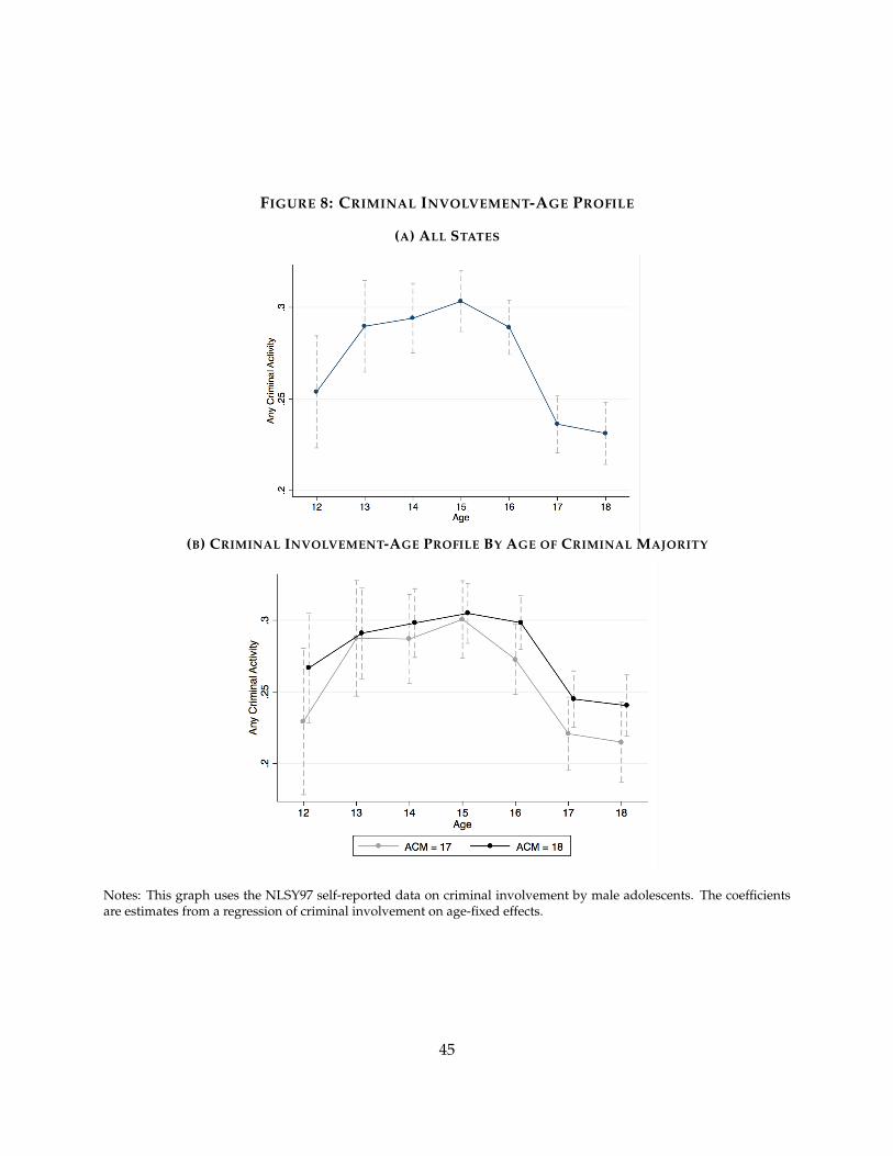
FIGURE 8: CRIMINAL INVOLVEMENT-AGE PROFILE

(A) ALL STATES

(B) CRIMINAL INVOLVEMENT-AGE PROFILE BY AGE OF CRIMINAL MAJORITY

Notes: This graph uses the NLSY97 self-reported data on criminal involvement by male adolescents. The coefficientsare estimates from a regression of criminal involvement on age-fixed effects.

45

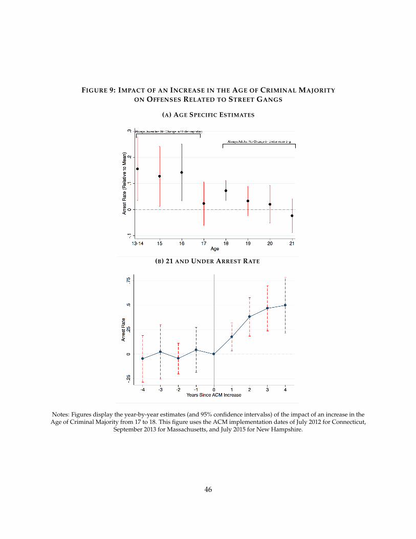
FIGURE 9: IMPACT OF AN INCREASE IN THE AGE OF CRIMINAL MAJORITYON OFFENSES RELATED TO STREET GANGS

(A) AGE SPECIFIC ESTIMATES

(B) 21 AND UNDER ARREST RATE

Notes: Figures display the year-by-year estimates (and 95% confidence intervalss) of the impact of an increase in theAge of Criminal Majority from 17 to 18. This figure uses the ACM implementation dates of July 2012 for Connecticut,

September 2013 for Massachusetts, and July 2015 for New Hampshire.

46

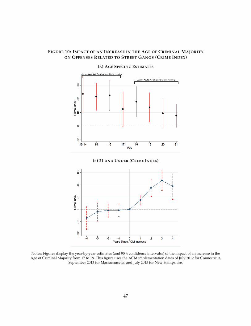
FIGURE 10: IMPACT OF AN INCREASE IN THE AGE OF CRIMINAL MAJORITYON OFFENSES RELATED TO STREET GANGS (CRIME INDEX)

(A) AGE SPECIFIC ESTIMATES

(B) 21 AND UNDER (CRIME INDEX)

Notes: Figures display the year-by-year estimates (and 95% confidence intervalss) of the impact of an increase in theAge of Criminal Majority from 17 to 18. This figure uses the ACM implementation dates of July 2012 for Connecticut,

September 2013 for Massachusetts, and July 2015 for New Hampshire.

47

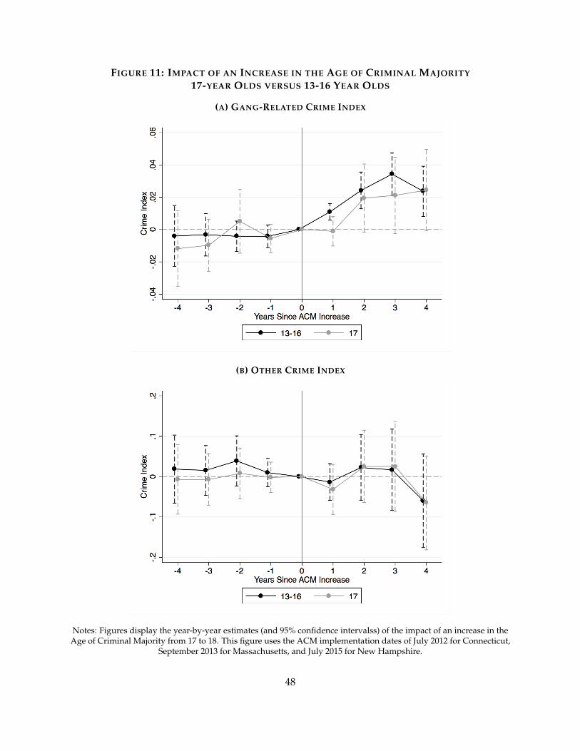
FIGURE 11: IMPACT OF AN INCREASE IN THE AGE OF CRIMINAL MAJORITY17-YEAR OLDS VERSUS 13-16 YEAR OLDS

(A) GANG-RELATED CRIME INDEX

(B) OTHER CRIME INDEX

Notes: Figures display the year-by-year estimates (and 95% confidence intervalss) of the impact of an increase in theAge of Criminal Majority from 17 to 18. This figure uses the ACM implementation dates of July 2012 for Connecticut,

September 2013 for Massachusetts, and July 2015 for New Hampshire.

48

Tables

TABLE 1: IMPACT OF AN INCREASE IN THE AGE OF CRIMINAL MAJORITYON JUVENILES AGED 13-17

Type of Offense All Gang-Related Other

Arrest Rate

DDD Estimate 0.310** 0.337*** -0.026(0.135) (0.109) (0.118)

Mean 5.438 3.925 1.301

Crime Index

DDD Estimate 0.003 0.019*** -0.013(0.015) (.003) (0.030)

Mean 0.004 -0.028 0.037

Observations 945,000 945,000 945,000Notes: Regressions estimate the impact of an increase in the Age of Criminal Majority from 17 to 18. Eachregression controls for state, year and age fixed effects, as well as state-year, age-year and age-state fixed

effects. Standard errors are clustered at the age-state level. *** p<0.01, ** p<0.05, * p<0.1.

49

TABLE 2: IMPACT BY AGE GROUP

Age Group Gang-Related Offenses Other OffensesArrest Rate Index Arrest Rate Index

13-14 0.242** 0.024*** -0.183* -0.015(0.101) (0.007) (0.103) (0.044)

Mean 1.695 -0.0240 0.346 0.0170

15 0.360** 0.022*** -0.219 -0.026(0.173) (0.005) (0.181) (0.041)

Mean 3.020 -0.0170 0.728 0.105

16 0.652** 0.023*** 0.032 -0.010(0.253) (0.006) (0.206) (0.045)

Mean 4.579 -0.0380 1.520 0.0120

17 0.160 0.012* 0.255 -0.007(0.270) (0.007) (0.377) (0.046)

Mean 6.327 -0.0330 2.612 0.0130

18 0.538*** 0.018*** 0.796 0.083(0.151) (0.006) (0.605) (0.152)

Mean 6.887 -0.0330 4.020 0.413

19 0.246 0.014** 0.999 -0.009(0.193) (0.006) (0.617) (0.060)

Mean 6.520 -0.0360 4.188 0.311

20 0.163 0.009* 0.909 0.015(0.232) (0.006) (0.574) (0.045)

Mean 5.803 -0.0380 3.911 0.209

21 -0.104 0.008* 0.432** -0.074(0.187) (0.004) (0.164) (0.305)

Mean 5.505 -0.0410 2.850 1.094

Observations 756,000 756,000 756,000 756,000Notes: Regressions estimate the impact of an increase in the Age of Criminal Majority from 17 to 18. Eachregression controls for state, year and age fixed effects, as well as state-year, age-year and age-state fixed

effects. Standard errors are clustered at the age-state level. *** p<0.01, ** p<0.05, * p<0.1.

50

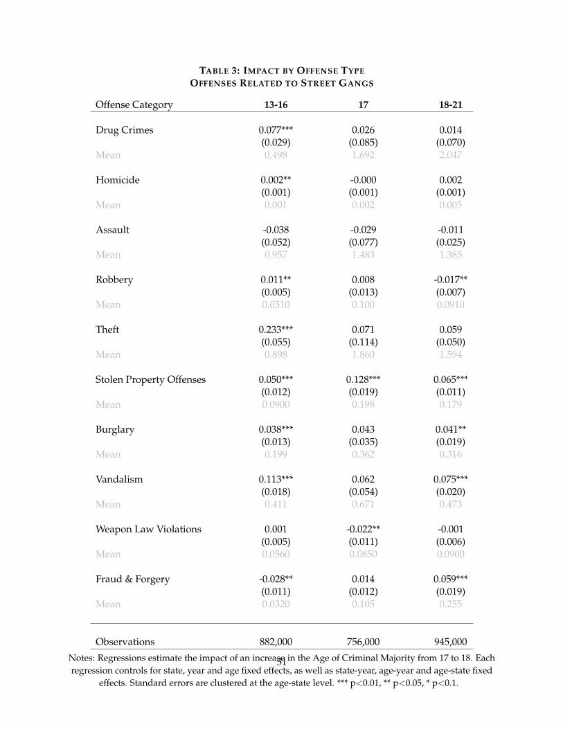
TABLE 3: IMPACT BY OFFENSE TYPEOFFENSES RELATED TO STREET GANGS

Offense Category 13-16 17 18-21

Drug Crimes 0.077*** 0.026 0.014(0.029) (0.085) (0.070)

Mean 0.498 1.692 2.047

Homicide 0.002** -0.000 0.002(0.001) (0.001) (0.001)

Mean 0.001 0.002 0.005

Assault -0.038 -0.029 -0.011(0.052) (0.077) (0.025)

Mean 0.957 1.483 1.385

Robbery 0.011** 0.008 -0.017**(0.005) (0.013) (0.007)

Mean 0.0510 0.100 0.0910

Theft 0.233*** 0.071 0.059(0.055) (0.114) (0.050)

Mean 0.898 1.860 1.594

Stolen Property Offenses 0.050*** 0.128*** 0.065***(0.012) (0.019) (0.011)

Mean 0.0900 0.198 0.179

Burglary 0.038*** 0.043 0.041**(0.013) (0.035) (0.019)

Mean 0.199 0.362 0.316

Vandalism 0.113*** 0.062 0.075***(0.018) (0.054) (0.020)

Mean 0.411 0.671 0.473

Weapon Law Violations 0.001 -0.022** -0.001(0.005) (0.011) (0.006)

Mean 0.0560 0.0850 0.0900

Fraud & Forgery -0.028** 0.014 0.059***(0.011) (0.012) (0.019)

Mean 0.0320 0.105 0.255

Observations 882,000 756,000 945,000Notes: Regressions estimate the impact of an increase in the Age of Criminal Majority from 17 to 18. Eachregression controls for state, year and age fixed effects, as well as state-year, age-year and age-state fixed

effects. Standard errors are clustered at the age-state level. *** p<0.01, ** p<0.05, * p<0.1.

51

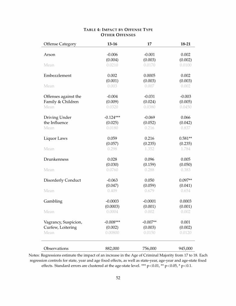
TABLE 4: IMPACT BY OFFENSE TYPEOTHER OFFENSES

Offense Category 13-16 17 18-21

Arson -0.006 -0.001 0.002(0.004) (0.003) (0.002)

Mean 0.0210 0.0170 0.0100

Embezzlement 0.002 0.0005 0.002(0.001) (0.003) (0.003)

Mean 0.003 0.007 0.002

Offenses against the -0.004 -0.031 -0.003Family & Children (0.009) (0.024) (0.005)Mean 0.0320 0.0380 0.0450

Driving Under -0.124*** -0.069 0.066the Influence (0.025) (0.052) (0.042)Mean 0.0180 0.216 0.837

Liquor Laws 0.059 0.216 0.581**(0.057) (0.235) (0.235)

Mean 0.298 1.352 1.784

Drunkenness 0.028 0.096 0.005(0.030) (0.159) (0.050)

Mean 0.0760 0.288 0.383

Disorderly Conduct -0.063 0.050 0.097**(0.047) (0.059) (0.041)

Mean 0.409 0.679 0.654

Gambling -0.0003 -0.0001 0.0003(0.0003) (0.001) (0.001)

Mean 0.0004 0.002 0.002

Vagrancy, Suspicion, -0.008*** -0.007** 0.001Curfew, Loitering (0.002) (0.003) (0.002)Mean 0.00800 0.0150 0.0120

Observations 882,000 756,000 945,000Notes: Regressions estimate the impact of an increase in the Age of Criminal Majority from 17 to 18. Eachregression controls for state, year and age fixed effects, as well as state-year, age-year and age-state fixed

effects. Standard errors are clustered at the age-state level. *** p<0.01, ** p<0.05, * p<0.1.

52

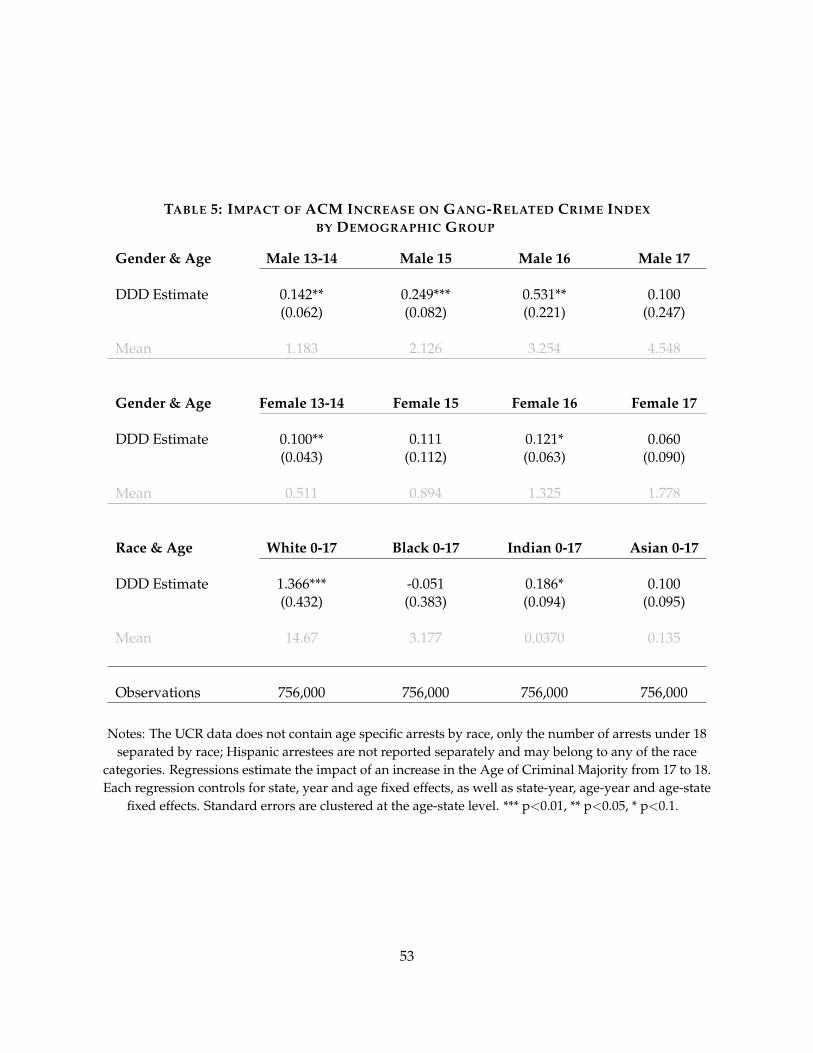
TABLE 5: IMPACT OF ACM INCREASE ON GANG-RELATED CRIME INDEXBY DEMOGRAPHIC GROUP

Gender & Age Male 13-14 Male 15 Male 16 Male 17

DDD Estimate 0.142** 0.249*** 0.531** 0.100(0.062) (0.082) (0.221) (0.247)

Mean 1.183 2.126 3.254 4.548

Gender & Age Female 13-14 Female 15 Female 16 Female 17

DDD Estimate 0.100** 0.111 0.121* 0.060(0.043) (0.112) (0.063) (0.090)

Mean 0.511 0.894 1.325 1.778

Race & Age White 0-17 Black 0-17 Indian 0-17 Asian 0-17

DDD Estimate 1.366*** -0.051 0.186* 0.100(0.432) (0.383) (0.094) (0.095)

Mean 14.67 3.177 0.0370 0.135

Observations 756,000 756,000 756,000 756,000

Notes: The UCR data does not contain age specific arrests by race, only the number of arrests under 18separated by race; Hispanic arrestees are not reported separately and may belong to any of the race

categories. Regressions estimate the impact of an increase in the Age of Criminal Majority from 17 to 18.Each regression controls for state, year and age fixed effects, as well as state-year, age-year and age-state

fixed effects. Standard errors are clustered at the age-state level. *** p<0.01, ** p<0.05, * p<0.1.

53

TABLE 6: SOCIAL COSTS OF INCREASE IN JUVENILE OFFENDING

Offense Arrest Rate Increase Arrest-Offense Unit Cost* Estimated Cost13-16-Year-Olds Ratio 2015 $ 2015 $

Homicide 0.005 61.5 9,717,787 255,060Robbery 0.038 29.3 41,842 17,689Aggravated Assault -0.055 54.0 115,383 -38,193Burglary 0.163 12.9 6,359 26,323MV Theft 0.035 13.1 11,241 9,709Larceny 0.451 21.9 3,706 24,929Stolen Property 0.159 19.4 7,526 20,112Vandalism 0.365 19.4 4,575 28,084Forgery 0.009 19.4 5,066 741Fraud -0.011 19.4 4,809 -892Drug Crimes 0.069 20.0 2,544 5,767

Total $ 264,953***

Notes: Arrest Rate Increase estimates are based on DDD regressions that estimate the impact of an increasein the Age of Criminal Majority from 17 to 18. Cost estimates are evaluated at a population of 27221, the

mean for treatment agencies. *** p<0.01, ** p<0.05, * p<0.1.

54

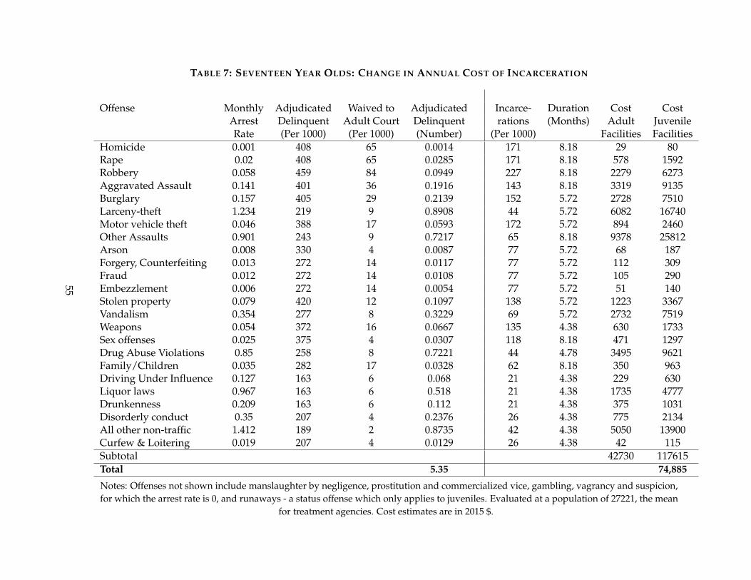
TABLE 7: SEVENTEEN YEAR OLDS: CHANGE IN ANNUAL COST OF INCARCERATION

Offense Monthly Adjudicated Waived to Adjudicated Incarce- Duration Cost CostArrest Delinquent Adult Court Delinquent rations (Months) Adult JuvenileRate (Per 1000) (Per 1000) (Number) (Per 1000) Facilities Facilities

Homicide 0.001 408 65 0.0014 171 8.18 29 80Rape 0.02 408 65 0.0285 171 8.18 578 1592Robbery 0.058 459 84 0.0949 227 8.18 2279 6273Aggravated Assault 0.141 401 36 0.1916 143 8.18 3319 9135Burglary 0.157 405 29 0.2139 152 5.72 2728 7510Larceny-theft 1.234 219 9 0.8908 44 5.72 6082 16740Motor vehicle theft 0.046 388 17 0.0593 172 5.72 894 2460Other Assaults 0.901 243 9 0.7217 65 8.18 9378 25812Arson 0.008 330 4 0.0087 77 5.72 68 187Forgery, Counterfeiting 0.013 272 14 0.0117 77 5.72 112 309Fraud 0.012 272 14 0.0108 77 5.72 105 290Embezzlement 0.006 272 14 0.0054 77 5.72 51 140Stolen property 0.079 420 12 0.1097 138 5.72 1223 3367Vandalism 0.354 277 8 0.3229 69 5.72 2732 7519Weapons 0.054 372 16 0.0667 135 4.38 630 1733Sex offenses 0.025 375 4 0.0307 118 8.18 471 1297Drug Abuse Violations 0.85 258 8 0.7221 44 4.78 3495 9621Family/Children 0.035 282 17 0.0328 62 8.18 350 963Driving Under Influence 0.127 163 6 0.068 21 4.38 229 630Liquor laws 0.967 163 6 0.518 21 4.38 1735 4777Drunkenness 0.209 163 6 0.112 21 4.38 375 1031Disorderly conduct 0.35 207 4 0.2376 26 4.38 775 2134All other non-traffic 1.412 189 2 0.8735 42 4.38 5050 13900Curfew & Loitering 0.019 207 4 0.0129 26 4.38 42 115Subtotal 42730 117615Total 5.35 74,885Notes: Offenses not shown include manslaughter by negligence, prostitution and commercialized vice, gambling, vagrancy and suspicion,for which the arrest rate is 0, and runaways - a status offense which only applies to juveniles. Evaluated at a population of 27221, the mean

for treatment agencies. Cost estimates are in 2015 $.

55

Appendix

A.11.1 Solving the ModelThis section calculates the the steady state values of kt and �t, and shows that the system exhibits saddlepath stability close to the steady state.

A.11.1.1 Steady State kt and �t

Dynamics in the model can be summarized by the following equations:

kt = ct � �kt =k↵t +�t

2st � �kt

�t = (⇢+ �)�t � ↵ctk1�↵t

At the adult steady state, kt = 0

ct = �kt =) �t = 2st�kt � k↵t

At the adult steady state, �t = 0 as well

(⇢+ �)�t =↵ctk1�↵t

Substituting in ct = �kt

(⇢+ �)�t = ↵k↵t

Using �t = 2st�kt � k↵t and assuming kSSA 6= 0

(⇢+ �)(2st�kt � k↵t ) = ↵k↵t

=) (⇢+ �)(2st�k1�↵t � 1) = ↵

=) kSSA = [ 12st� { ↵

(⇢+�) + 1}] 11�↵

The steady state value of criminal capital decreases in criminal sanctions s, depreciation rate � and the rate atwhich future utility is discounted �. However, kSSA increases with the returns to additional criminal capital,represented by ↵.

A.11.1.2 Saddle Path Stability

To show that the system of differential equations exhibits saddle path stability, I use a first order Taylorapproximation to linearize the system around the steady state values. This system can be written in matrixform:

kt�t

�⇡

"↵(⇢+�)�(↵+⇢+�)

↵+⇢+�1

2st(1� 2↵)(⇢+ �) + ↵(1� ↵) (⇢+ �)(1� �↵

↵+⇢+� )

# kt � k⇤

�t � �⇤

�= [A]

kt � k⇤

�t � �⇤

�

The necessary and sufficient condition for saddle-path stability is that the determinant of A is negative. Thiscondition is met if 0 < ↵ < 1

2 since

56

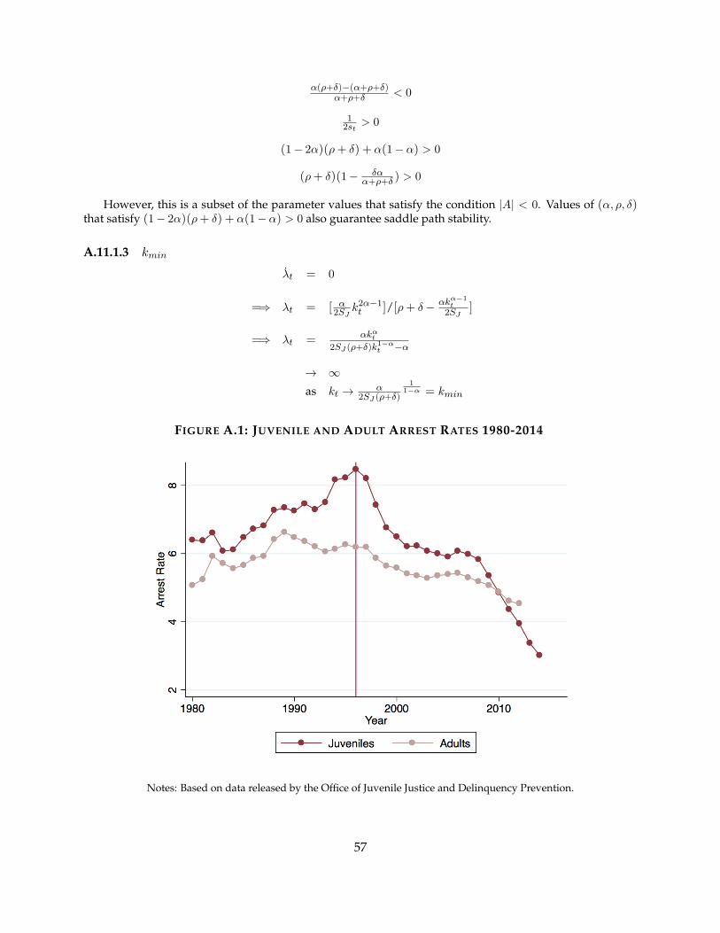
↵(⇢+�)�(↵+⇢+�)↵+⇢+� < 0

12st > 0

(1� 2↵)(⇢+ �) + ↵(1� ↵) > 0

(⇢+ �)(1� �↵↵+⇢+� ) > 0

However, this is a subset of the parameter values that satisfy the condition |A| < 0. Values of (↵, ⇢, �)that satisfy (1� 2↵)(⇢+ �) + ↵(1� ↵) > 0 also guarantee saddle path stability.

A.11.1.3 kmin

�t = 0

=) �t = [ ↵2SJ

k2↵�1t ]/[⇢+ �� ↵k↵�1

t2SJ

]

=) �t = ↵k↵t2SJ (⇢+�)k1�↵

t �↵

! 1as kt ! ↵

2SJ (⇢+�)

11�↵ = kmin

FIGURE A.1: JUVENILE AND ADULT ARREST RATES 1980-2014

Notes: Based on data released by the Office of Juvenile Justice and Delinquency Prevention.

57

FIGURE A.2: PROPORTION OF OFFENSES BY AGE 2006-14

(A) AGE OF CRIMINAL RESPONSIBILITY = 17

(B) AGE OF CRIMINAL RESPONSIBILITY = 18

Notes: This graph uses monthly data at the law enforcement agency level from 39 states in the NIBRS data. Confidenceintervals are shown in red.

58

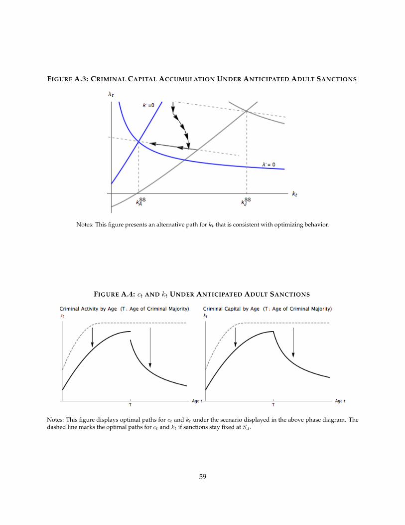
FIGURE A.3: CRIMINAL CAPITAL ACCUMULATION UNDER ANTICIPATED ADULT SANCTIONS

Notes: This figure presents an alternative path for kt

that is consistent with optimizing behavior.

FIGURE A.4: ct AND kt UNDER ANTICIPATED ADULT SANCTIONS

Notes: This figure displays optimal paths for ct

and kt

under the scenario displayed in the above phase diagram. Thedashed line marks the optimal paths for c

t

and kt

if sanctions stay fixed at SJ

.

59

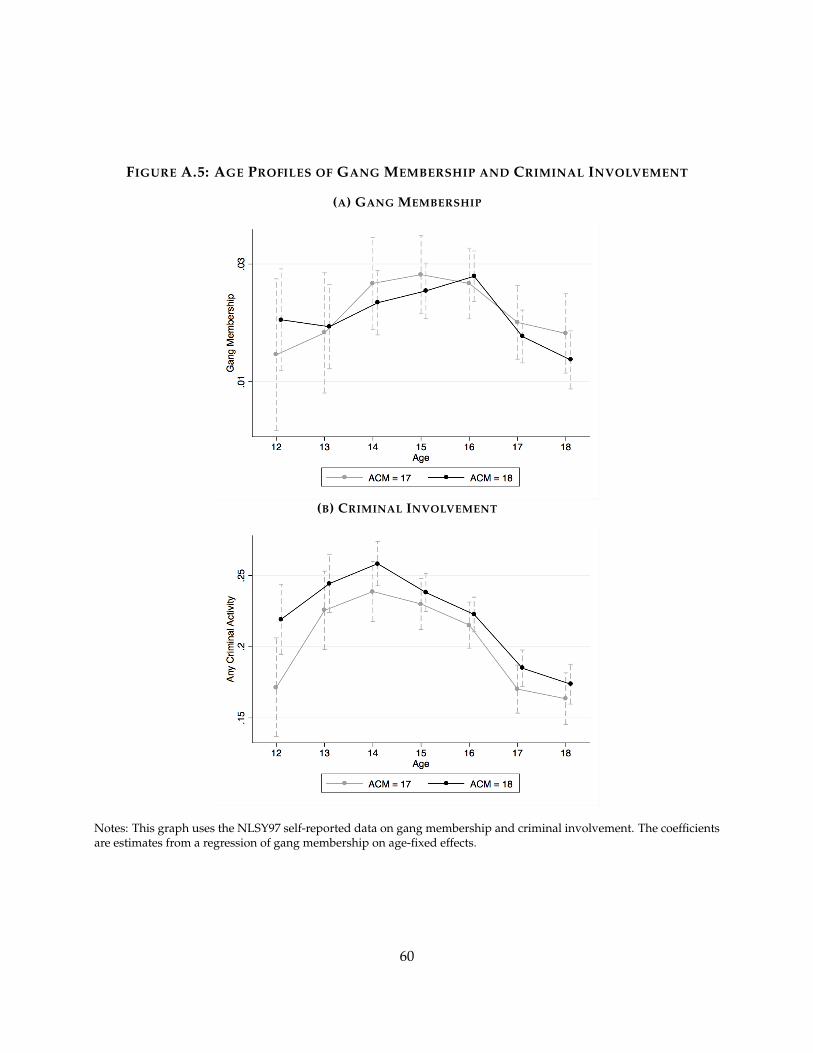
FIGURE A.5: AGE PROFILES OF GANG MEMBERSHIP AND CRIMINAL INVOLVEMENT

(A) GANG MEMBERSHIP

(B) CRIMINAL INVOLVEMENT

Notes: This graph uses the NLSY97 self-reported data on gang membership and criminal involvement. The coefficientsare estimates from a regression of gang membership on age-fixed effects.

60

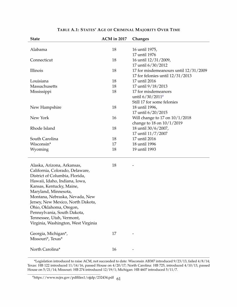
TABLE A.1: STATES’ AGE OF CRIMINAL MAJORITY OVER TIME

State ACM in 2017 Changes

Alabama 18 16 until 1975,17 until 1976

Connecticut 18 16 until 12/31/2009,17 until 6/30/2012

Illinois 18 17 for misdemeanours until 12/31/200917 for felonies until 12/31/2013

Louisiana 18 17 until 2016Massachusetts 18 17 until 9/18/2013Mississippi 18 17 for misdemeanors

until 6/30/2011a

Still 17 for some feloniesNew Hampshire 18 18 until 1996,

17 until 6/20/2015New York 16 Will change to 17 on 10/1/2018

change to 18 on 10/1/2019Rhode Island 18 18 until 30/6/2007,

17 until 11/7/2007South Carolina 18 17 until 2016Wisconsin* 17 18 until 1996Wyoming 18 19 until 1993

Alaska, Arizona, Arkansas, 18 -California, Colorado, Delaware,District of Columbia, Florida,Hawaii, Idaho, Indiana, Iowa,Kansas, Kentucky, Maine,Maryland, Minnesota,Montana, Nebraska, Nevada, NewJersey, New Mexico, North Dakota,Ohio, Oklahoma, Oregon,Pennsylvania, South Dakota,Tennessee, Utah, Vermont,Virginia, Washington, West Virginia

Georgia, Michigan*, 17 -Missouri*, Texas*

North Carolina* 16 -

*Legislation introduced to raise ACM, not succeeded to date: Wisconsin AB387 introduced 9/23/13, failed 4/8/14;Texas: HB 122 introduced 11/14/16, passed House on 4/20/17; North Carolina: HB 725, introduced 4/10/13, passedHouse on 5/21/14; Missouri: HB 274 introduced 12/19/1; Michigan: HB 4607 introduced 5/11/7.

ahttps://www.ncjrs.gov/pdffiles1/ojjdp/232434.pdf 61

TABLE A.2: JURISDICTIONS BORDERING TREATMENT AND CONTROL STATES

State Border Municipalities Police Agencies

Connecticut Salisbury, Sharon, Kent, Sherman, Connecticut State Police, Danbury,New Fairfield, Danbury, Ridgefield, Wilton, Ridgefield, Wilton, New Canaan,New Canaan, Stamford, Greenwich Stamford, Greenwich

Massachusetts Williamstown, Hancock, Richmond, West Wiliamstown, Egremont, StateStockbridge, Alford, Edgemont, Mount Police: Berkshire County, StateWashington, Clarksburg, Monroe, Florida, Police: Franklin County,Rowe, Heath, Colrain, Leyden, Bernardston, BernardstonNorthfield

New York Petersburg, Berlin, Stephentown, Northeast Millerton, Rensselaer, Brewster,(Millerton), Amenia, Dover, Pawling, Patterson, Lewisboro, Pound Ridge, NorthSoutheast (Brewster), North Salem, Lewisboro, Castle, Harrison, RyeBrook, PortPound Ridge, North Castle, Harrison, Rye Chester, Dutchess, Putnam,Brook, Port Chester Westchester Public Safety

Vermont Canaan, Lemington, Bloomfield, Brunswick, Canaan, State Police: St. Johnsbury,Maidstone, Guildhall, Lunenburo, Concord, Bradford, Thetford, Norwich, Hartford,Waterford, Barnet, Rye Gate, Newbury, Bradford, State Police: Royalton, Windsor,Fairlee, Thetford, Norwich, Hartford, Hartland, Weathersfield, Springfield, State Police:Windsor, Weathersfield, Springfield, Rockingham, Bratteboro, Bratteboro, Vernon, StateWestminster, Putney, Dummerston, Brattleboro, Police: ShaftsburyVernon, Guilford, Halifax, Whitingham,Readsboro, Stamford, Pownal

62

TABLE A.3: ROBUSTNESS CHECKS: IMPACT OF AN INCREASE IN THE AGE OF CRIMINAL MAJORITYON JUVENILE ARREST RATE FOR GANG RELATED OFFENSES

Sample 6 NE States 6 NE States 6 NE States 6 NE States 5 NE States 9 NE States Entire USa

Excl. Boundary (Excl. CT)Jurisdictions

DDD Estimate 0.337 0.453 0.221 0.338 0.490 0.484 0.540(0.109)*** (0.105)*** (0.110)** (0.114)*** (0.136)*** (0.126)*** (0.152)***

95% C.I. [0.123, 0.551] [0.242, 0.664] [0.002, 0.440] [0.114, 0.562] [0.222, 0.765] [0.237, 0.731] [0.242, 0.838]Clustering Level:Age-State

95% C.I. [0.097, 0.592] [0.261, 0.668] [ -0.054, 0.494] [0.109, 0.573] [0.243, 0.734] [0.143, 0.851] [0.058,1.022]Clustering Level:Juvenile-State

Mean 3.925 3.925 3.925 3.971 3.927 4.259 5.235

Control Age Groups [22, 65) [22, 30) [30, 65) [22, 65) [22, 65) [22, 65) [22, 65)Observations 945,000 504,000 693,000 916,200 817,200 2,453,400 8,314,200

Notes: Regressions estimate the impact of an increase in the Age of Criminal Majority from 17 to 18. Juveniles are defined as 13-17-year-olds.Confidence intervals are estimated using the wild bootstrap when the number of clusters is below thirty. *** p<0.01, ** p<0.05, * p<0.1.

aSample consists of 49 states in the UCR

63

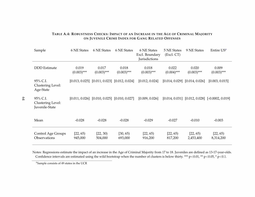
TABLE A.4: ROBUSTNESS CHECKS: IMPACT OF AN INCREASE IN THE AGE OF CRIMINAL MAJORITYON JUVENILE CRIME INDEX FOR GANG RELATED OFFENSES

Sample 6 NE States 6 NE States 6 NE States 6 NE States 5 NE States 9 NE States Entire USa

Excl. Boundary (Excl. CT)Jurisdictions

DDD Estimate 0.019 0.017 0.018 0.018 0.022 0.020 0.009(0.003)*** (0.003)*** (0.003)*** (0.003)*** (0.004)*** (0.003)*** (0.003)***

95% C.I. [0.013, 0.025] [0.011, 0.023] [0.012, 0.024] [0.012, 0.024] [0.014, 0.029] [0.014, 0.026] [0.003, 0.015]Clustering Level:Age-State

95% C.I. [0.011, 0.026] [0.010, 0.025] [0.010, 0.027] [0.009, 0.026] [0.014, 0.031] [0.012, 0.028] [-0.0002, 0.019]Clustering Level:Juvenile-State

Mean -0.028 -0.028 -0.028 -0.029 -0.027 -0.010 -0.003

Control Age Groups [22, 65) [22, 30) [30, 65) [22, 65) [22, 65) [22, 65) [22, 65)Observations 945,000 504,000 693,000 916,200 817,200 2,453,400 8,314,200

Notes: Regressions estimate the impact of an increase in the Age of Criminal Majority from 17 to 18. Juveniles are defined as 13-17-year-olds.Confidence intervals are estimated using the wild bootstrap when the number of clusters is below thirty. *** p<0.01, ** p<0.05, * p<0.1.

aSample consists of 49 states in the UCR

64

Chapter 2

The Career Impact of First Jobs:

Evidence and Labor Market Design Lessons from Randomized Choice Sets⇤

Ashna Arora† Jonas Hjort‡

Abstract

We study the impact of a graduate’s first job on her career trajectory; job-seeking graduates’

response; and how policy rules’ impact on worker-job matches ultimately helps shape the dis-

tribution of realized “first job effects” (FJEs). In Norway, doctors’ first job—their residency—is

allocated through a random serial dictatorship (RSD) mechanism. We first exploit the resulting

random variation in individual doctors’ choice sets to estimate each type of job characteristic’s

impact on long-run earnings, place of residence, and specialization for each type of individual.

We then account for these FJEs when estimating each worker type’s preferences over job char-

acteristics, enabling us to decompose the long-term consequences of a particular choice set into

a component that is due to chance and a component that is due to workers’ preference-driven

response. Finally, we exploit the replacement of the RSD mechanism with decentralized job-

finding in 2013 to show how total worker welfare and the distribution of realized FJEs across

worker types—due to changes in worker-job matches—differ in a market system relative to

RSD. To our knowledge, these findings represent the first causal evidence on the career impact

of individual level variation in first jobs and the challenges and opportunities they present for

graduates and policymakers.

⇤aa3332@columbia.edu, hjort@columbia.edu. We thank Josh Angrist, Chris Conlon, Francois Gerard, Adam Kapor,

José Luis Montiel Olea, Ben Olken, Parag Pathak, Jonah Rockoff, and Till von Wachter for helpful suggestions. We are

especially grateful to Andreas Fagereng, with whom we started this project. The project received funding from the

Research Council of Norway (#256678).†Columbia University & Statistics Norway‡Columbia University & CEPR & NBER

65

1 Introduction

An individual’s first job may have important consequences for her career trajectory. This view—

common among researchers—appears widely held also among those entering the labor market.1

New job-seekers may therefore put weight on the expected impact of different jobs on their trajec-

tories when choosing a first job to pursue. Policy, on the other hand—whether centralized mech-

anisms allocating doctors, teachers, and other groups of workers serving the public to first jobs2,

or the rules and regulations that influence initial worker-job matches in the decentralized labor

market—is typically designed without accounting for expected “first job effects” (FJEs). If FJEs

are non-negligible in magnitude and heterogeneous across types of workers, then FJE-responsive

policy design may increase welfare. However, even in such a scenario, whether alternative policies

actually affect initial worker-job matches—and hence realized FJEs—differentially is an empirical

question. Unusual types of data and variation are necessary for researchers to be able to identify

FJEs and graduates’ and policymakers’ actual and ideal response. To estimate the causal, long-

term effect of an individual’s first job, random variation in her match, holding all else constant,

is needed. To go beyond such a LATE and estimate how individuals’ distribution of FJEs across

jobs influence their job search choices, causal estimates of the long-term effect of each type of job

for each type of individual—and knowledge of individuals’ choice set when entering the labor

market—are needed.

In this paper we take advantage of Norway’s 1997-2013 allocation of doctors’ first job—their

residency—through a Random Serial Dictatorship (RSD) mechanism3, and the replacement of the

RSD with decentralized job-finding in 2013, to overcome these challenges. We first estimate the

consequences for earnings, place of residence, and specialization in the long-term of each type of

job characteristic for each type of individual. We do so by exploiting RSD-generated random, indi-

vidual level variation in new doctors’ choice sets over jobs. We then account for these FJEs when

1The influential studies by Genda et al. (2010); Heisz et al. (2012); Kahn (2010); Oyer (2006, 2008) all documentpersistent career effects for cohorts of new workers that graduate in a weak labor market.

2The following is an incomplete list of countries that use centralized mechanisms to assign workers in some (in someof the countries, almost all) public service occupations to first jobs: Australia, Bangladesh, Bhutan, Botswana, Canada,Denmark, France, Ghana, India, Iran, Ireland, Israel, Italy, Japan, Malaysia, Malta, Nepal, Norway, Pakistan, Philipines,Saudi Arabia, Senegal, Singapore, South Africa, South Korea, Taiwan, Tanzania, Uganda, U.K., USA.

3A Random Serial Dictatorship mechanism starts with a lottery. The person who draws number 1 then chooses herpreferred object freely among all available options. After that, the person who draws number 2 chooses among theremaining objects, and so on.

66

estimating each type of individual’s preferences over (short- and long-term) job characteristics.

The unique suitability of doctors’ residencies in Norway for studying FJEs is due to the com-

bination of choice sets over jobs being assigned randomly, and the unusually high quality of the

registry data available on the universe of Norwegian workers. While our quantitative results may

not generalize to other occupations, it is worth noting that (i) the differences between the possible

pathways a doctor’s career can take share many features with those in other occupations4, and

(ii) the literature generally finds that highly skilled workers are least affected by temporary ca-

reer shocks (Oreopoulos et al. , 2012; von Wachter & Bender, 2006). Most likely our results thus

represent a lower bound on FJEs and the associated responses in other occupations.

This paper contributes to the literature on how temporary shocks to a worker’s employment

status affects her career trajectory. Existing studies have convincingly and carefully documented

the consequences of job displacement (see, among many others, Bender et al. , 2009; Sullivan &

von Wachter, 2009; von Wachter & Bender, 2006); exposure to high unemployment rates later in

life (Coile et al. , 2012); and, most closely related to this paper, graduating in a weak labor market

(Genda et al. , 2010; Heisz et al. , 2012; Kahn, 2010; Oyer, 2006, 2008). These influential studies

have shown how cohort and group-level labor market shocks affect individual workers’ trajecto-

ries.5 In addition to taking advantage of an explicit randomization for identification, this paper

to our knowledge provides the first causal evidence on the career consequences of individual level

shocks to a graduate’s first job. The distinction is essential because cohort level studies may not

be informative about the career consequences of individual level labor market shocks, which are

ubiquitous. When the cohort or group an individual belongs to is hit, for example, by a reces-

sion or a mass layoff, then the individual’s peers are also affected. Peers’ exposure to the shock

could adversely affect the trajectory of the individual in question (if for example she now faces

more competition for current jobs) or benefit her (if for example she’s now competing against less

employable other workers for future jobs).6

4For example, doctors’ jobs are located in many different parts of a country; there is considerable dispersion in em-ployer size and "quality" (which is highly correlated with doctors’ earned income); and there are ample opportunities fordoctors to undertake horizontal specialization (choice of medical field) as well as vertical specialization (e.g. becominga specialist as opposed to a General Practitioner).

5To our knowledge, the only existing causal evidence on the long-term effects of individual level shocks to first jobscomes from Angrist (1990)’s seminal study of the Vietnam draft. He shows that being drafted lowered earnings by 15percent long after the veterans’ service ended (see also Angrist, 1995; Angrist & Chen, 2011).

6Ruhm (2000) shows that mortality tends to improve during recessions, while Sullivan & von Wachter (2009) showthat own job displacements increase mortality for U.S. workers.

67

Our second contribution is to identify how graduates respond to variation in the labor market

they face. To do so we estimate graduates’ preferences over job characteristics. What allows us

to do so is the fact that we observe each graduate’s complete choice set over jobs, and that the

choice set is de facto randomly determined. With estimates of graduates’ preferences in hand

we can decompose the long-term consequences of a particular choice set into a component that

is due to chance and a component that is due to workers’ response. This allows us to estimate

how graduates’ welfare is affected by labor market shocks. The existing literature has studied

the impact of recessions, displacement, and other temporary shocks on particular components of

workers’ future welfare, such as income. These impacts are important, but do not tell the complete

story since workers value other job characteristics as well.7

The paper is organized as follows. In Section 2 we discuss background on the setting and insti-

tutional setup. In Section 3 we present the datasets used in our empirical analysis. In Section 4 we

lay out our empirical strategy. Section 5 estimates doctor preferences for residency characteristics,

shows how residency characteristics influence doctors’ careers in the long term, and how doctors

account for these long-term effects when choosing a residency hospital. Section 6 concludes.

2 Setting

2.1 The Random Serial Dictatorship mechanism for Norwegian doctors

The “turnus” (roster) system that was used to match medical graduates with residency positions

in Norway from 1954 to 2013 was a Random Serial Dictatorship (RSD) mechanism. Theorists

have shown that, among other important properties, the RSD is incentive-compatible, inducing

participants to reveal their true preferences (Abdulkadiroglu & Sönmez, 1998).

Equitable access to primary healthcare across regions was the main motivation behind the use

of a lottery system in Norway. Like other countries, Norway had had trouble filling doctor va-

cancies in rural areas, and the RSD mechanism was expected to distribute the best doctors more

equally across space. In addition, the mechanism appealed to policymakers because it was per-

7This paper is of course not the first to recognize that workers care about non-income job characteristics and maychoose occupations and employers partly based on those preferences. Recently, for example, Sorkin (2016) showedevidence of compensating differentials revealed in workers’ job-to-job transitions in the U.S.

68

ceived to be fair to the participating medical graduates.8

First, graduating students would enter a lottery, either in February or in August, and be as-

signed a random draw number. Next, the student with the lowest draw number would choose

freely between all available positions. Next, the student with the second lowest draw number

would choose from the remaining residency positions. This would continue until the student with

the highest draw number remained, who would take whichever spot was available.9

Three categories of new doctors received special treatment: couples, who were allowed to draw

a shared lottery draw number and to choose residencies simultaneously; doctors with children;

and doctors with maternity or health issues. The latter two categories were allowed to choose

between positions deemed especially suitable for them before the lottery took place. Since these

three types of doctors were not subject to randomization via the lottery, we exclude them from our

analysis.

In the late 2000s, the system began to concern the government, because of the growth of the

number of applicants and the rise in proportion of students from foreign universities.10 The num-

ber of medical graduates participating in the lottery would routinely exceed the number of training

positions available. As a result, it became increasingly difficult for the government to guarantee

a six-month maximum waiting time to obtain a residency. In 2013, the Norwegian Health Minis-

ter replaced the lottery system with direct qualification after six years of medical school. Medical

graduates now apply to residencies directly, as in a regular labor market, and hospital trusts are

responsible for selection and recruitment.

2.2 Doctors in Norway 1995-2014

This section profiles doctors that worked in Norway during the study period; we go through the

data we use in detail in Section 3. Medical students in Norway begin their studies in the Fall or

Spring semester, and usually take ten semesters to graduate. Starting in the 1950s, the Norwegian

government mandated an eighteen month residency period, after which medical school graduates8The government also wished to incentivize doctors to work in rural locations in other ways. For instance, doctors

who agreed to intern at hospitals in the largely rural counties of Sogn og Fjordande and Finnmark could skip the lotteryentirely.

9If the number of students exceeded the number of residency positions, the unassigned students would get priorityin the next lottery.

10Norway was compelled by its participation in the EU common labor market system to accept any European medicalgraduate who could pass a Norwegian language test into the system.

69

could become fully licensed physicians and practice independently. The first twelve months were

to be spent at a hospital, while the remaining six months were to be spent as a General Practitioner

(i.e. one who works in Primary Care) within the same county.11

Table 2 summarizes a range of socioeconomic information on doctors including age, proportion

born abroad, proportion that studied abroad, family size, field of specialization and income and

assets. The last two columns summarize this information separately for men and women. Women

comprise over 40 percent of doctors, and tend to be over-represented in fields like gynecology

and psychiatry. Male doctors are older and tend to be over-represented in fields like surgery and

internal medicine. A fifth of all doctors were born abroad, of which an overwhelming proportion

are citizens of Denmark and Sweden. Finally, recorded income, asset and debt holdings are higher

on average for male doctors.

There are 30 basic medical specialties, and specialization is usually in the form of training on

the job.12 The average length of time required to complete a specialty is five years, but it can take

longer with large variations between the specialties. Figure A.4 indicates that there appear to be

substantial returns to specializing—job retention rates are higher for specialists, and the salary

bump from specialization increases with age. In Section 5 we show that residency characteristics

significantly impact when and whether doctors become specialists.

2.3 Hospitals in Norway 1995-2014

The employer-employee database contains information on all registered employers that employ

doctors in Norway.13 Figure A.3 depicts the steady growth in both the number of hospitals and

average hospital size (number of doctors employed) since 1995.

Hospitals vary across multiple dimensions. Table 1 summarizes information on salaries, geo-

graphical remoteness, number of doctors and other medical staff, proportion of specialists, as well

as the presence of fifteen distinct specialist fields. Most hospitals in Norway are located in urban

municipalities; on average, municipalities with hospitals have only 10 per cent of their popula-

tion living in rural areas. This is noteworthy because the average municipality in Norway had 4911The last six months could be spent at an institution that was disjoint from the hospital of the first twelve months.12The Norwegian Medical Association evaluates whether the candidate has met the requirements to become a spe-

cialist. Specialist titles are formally awarded by the Health Directorate.13We define hospitals as employers that hire at least 10 doctors. These account for around 80 per cent of doctor

employment.

70

percent of its population living in rural areas.

Table A.1 shows how seven major hospital characteristics vary with one another. Salaries are

typically higher at hospitals that are more specialized. Average salary also increases with remote-

ness of location.

Post-residency salaries may be used both to compensate doctors to work in less desirable hos-

pitals, and also to attract the best doctors. We now shed some light on how salaries vary with

individual and hospital characteristics by estimating the following equation:

S

iht

= �0 + �Xht +!Zit + �

t

+ "

iht

S

iht

is the salary paid to doctor i by hospital h in year t, and X

ht

is a vector of time-varying hospital

characteristics. Zht is a vector of time varying individual-level characteristics like age, sex, citizen-

ship and choice of specialization (if any). �t

are year fixed effects. Table A.2 displays the estimates

for � and !. Hospitals that are more specialized and located in rural areas pay higher salaries. We

include dummies for four categories of hospital size and find that salaries increase with hospital

size even within hospitals that employ less than 10 doctors. Turning to individual characteristics,

we find that male doctors and those born in Norway earn higher salaries on average. The highest

paying specialties include anesthiology, gynaecology, surgery and diagnostic medicine.

3 Data

We combine information on lottery outcomes with Norwegian administrative data from 1993 to

2013. We obtained information on lottery draw numbers for all lottery participants who were

assigned a residency position during 1993-2013 from the Norwegian Registration Authority for

Health Personnel (SAFH). This information was linked with the employer-employee registry to

match medical graduates to their residency hospitals, as well as employer information in the years

following the residency. This data was then linked to administrative registers provided by Statis-

tics Norway, a rich longitudinal database that includes information on medical graduates’ socioe-

conomic information (sex, age, marital status, educational attainment, specialization, income, and

gross wealth), geographical identifiers and year-end asset holdings and liabilities (such as real es-

tate, stock holdings, etc) for each year. These data have several valuable attributes. There is no

71

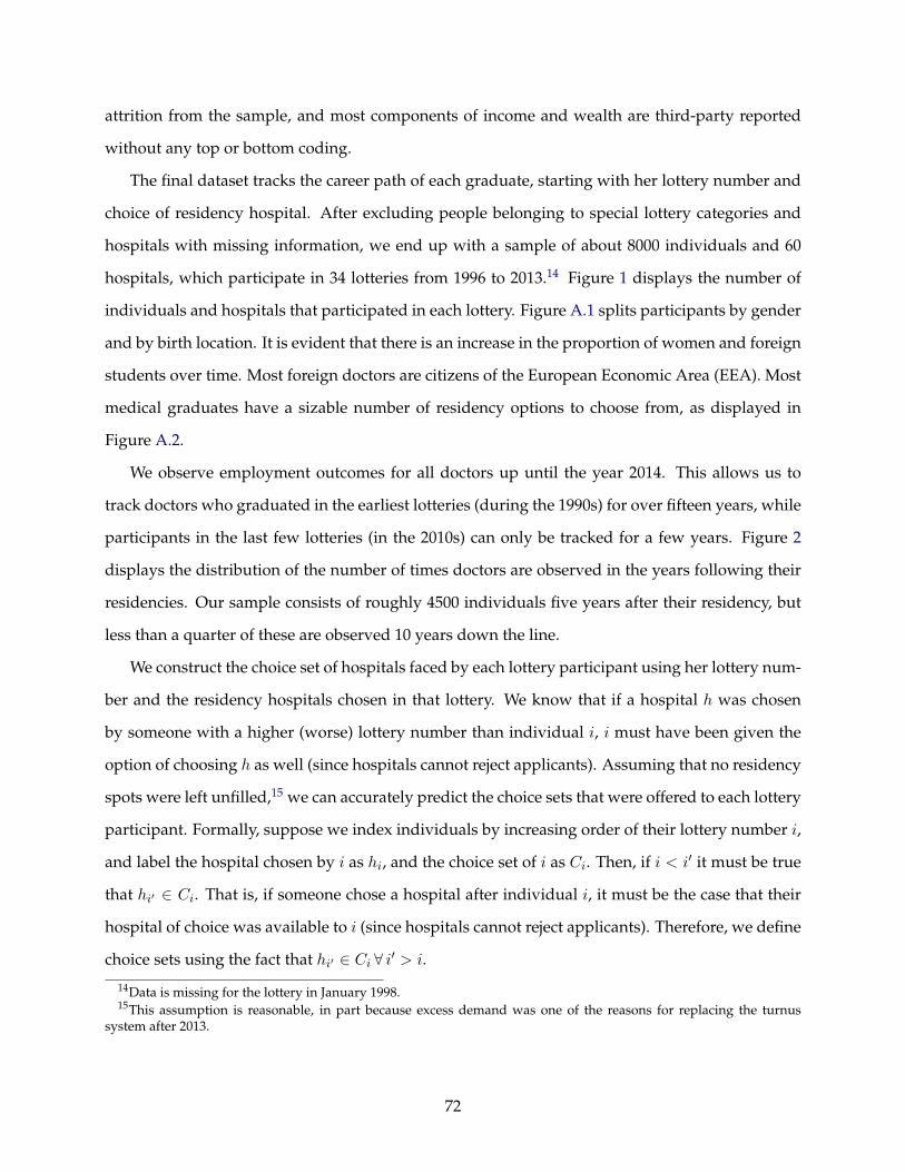
attrition from the sample, and most components of income and wealth are third-party reported

without any top or bottom coding.

The final dataset tracks the career path of each graduate, starting with her lottery number and

choice of residency hospital. After excluding people belonging to special lottery categories and

hospitals with missing information, we end up with a sample of about 8000 individuals and 60

hospitals, which participate in 34 lotteries from 1996 to 2013.14 Figure 1 displays the number of

individuals and hospitals that participated in each lottery. Figure A.1 splits participants by gender

and by birth location. It is evident that there is an increase in the proportion of women and foreign

students over time. Most foreign doctors are citizens of the European Economic Area (EEA). Most

medical graduates have a sizable number of residency options to choose from, as displayed in

Figure A.2.

We observe employment outcomes for all doctors up until the year 2014. This allows us to

track doctors who graduated in the earliest lotteries (during the 1990s) for over fifteen years, while

participants in the last few lotteries (in the 2010s) can only be tracked for a few years. Figure 2

displays the distribution of the number of times doctors are observed in the years following their

residencies. Our sample consists of roughly 4500 individuals five years after their residency, but

less than a quarter of these are observed 10 years down the line.

We construct the choice set of hospitals faced by each lottery participant using her lottery num-

ber and the residency hospitals chosen in that lottery. We know that if a hospital h was chosen

by someone with a higher (worse) lottery number than individual i, i must have been given the

option of choosing h as well (since hospitals cannot reject applicants). Assuming that no residency

spots were left unfilled,15 we can accurately predict the choice sets that were offered to each lottery

participant. Formally, suppose we index individuals by increasing order of their lottery number i,

and label the hospital chosen by i as hi

, and the choice set of i as Ci

. Then, if i < i

0 it must be true

that hi

0 2 C

i

. That is, if someone chose a hospital after individual i, it must be the case that their

hospital of choice was available to i (since hospitals cannot reject applicants). Therefore, we define

choice sets using the fact that hi

0 2 C

i

8 i0 > i.

14Data is missing for the lottery in January 1998.15This assumption is reasonable, in part because excess demand was one of the reasons for replacing the turnus

system after 2013.

72

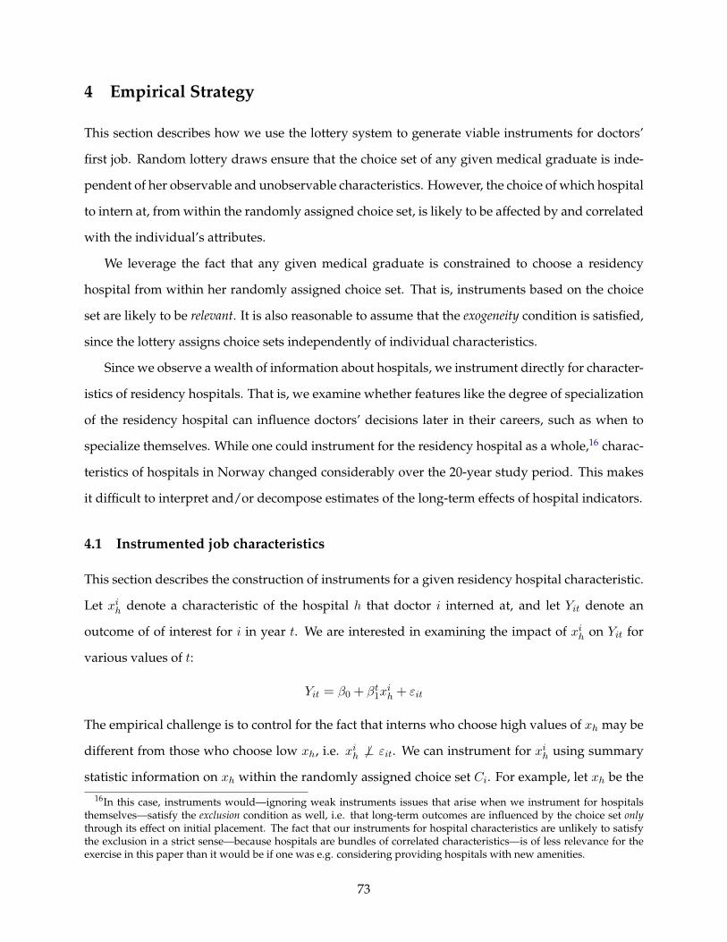
4 Empirical Strategy

This section describes how we use the lottery system to generate viable instruments for doctors’

first job. Random lottery draws ensure that the choice set of any given medical graduate is inde-

pendent of her observable and unobservable characteristics. However, the choice of which hospital

to intern at, from within the randomly assigned choice set, is likely to be affected by and correlated

with the individual’s attributes.

We leverage the fact that any given medical graduate is constrained to choose a residency

hospital from within her randomly assigned choice set. That is, instruments based on the choice

set are likely to be relevant. It is also reasonable to assume that the exogeneity condition is satisfied,

since the lottery assigns choice sets independently of individual characteristics.

Since we observe a wealth of information about hospitals, we instrument directly for character-

istics of residency hospitals. That is, we examine whether features like the degree of specialization

of the residency hospital can influence doctors’ decisions later in their careers, such as when to

specialize themselves. While one could instrument for the residency hospital as a whole,16 charac-

teristics of hospitals in Norway changed considerably over the 20-year study period. This makes

it difficult to interpret and/or decompose estimates of the long-term effects of hospital indicators.

4.1 Instrumented job characteristics

This section describes the construction of instruments for a given residency hospital characteristic.

Let x

i

h

denote a characteristic of the hospital h that doctor i interned at, and let Y

it

denote an

outcome of of interest for i in year t. We are interested in examining the impact of xih

on Y

it

for

various values of t:

Y

it

= �0 + �

t

1xi

h

+ "

it

The empirical challenge is to control for the fact that interns who choose high values of xh

may be

different from those who choose low x

h

, i.e. x

i

h

6? "

it

. We can instrument for x

i

h

using summary

statistic information on x

h

within the randomly assigned choice set Ci

. For example, let xh

be the16In this case, instruments would—ignoring weak instruments issues that arise when we instrument for hospitals

themselves—satisfy the exclusion condition as well, i.e. that long-term outcomes are influenced by the choice set onlythrough its effect on initial placement. The fact that our instruments for hospital characteristics are unlikely to satisfythe exclusion in a strict sense—because hospitals are bundles of correlated characteristics—is of less relevance for theexercise in this paper than it would be if one was e.g. considering providing hospitals with new amenities.

73

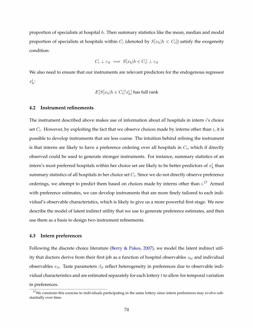
proportion of specialists at hospital h. Then summary statistics like the mean, median and modal

proportion of specialists at hospitals within C

i

(denoted by S[xh

|h 2 C

i

]) satisfy the exogeneity

condition:

C

i

? "

it

=) S[xh

|h 2 C

i

] ? "

it

We also need to ensure that our instruments are relevant predictors for the endogenous regressor

x

i

h

:

E[S[xh

|h 2 C

i

]0xih

] has full rank

4.2 Instrument refinements

The instrument described above makes use of information about all hospitals in intern i’s choice

set Ci

. However, by exploiting the fact that we observe choices made by interns other than i, it is

possible to develop instruments that are less coarse. The intuition behind refining the instrument

is that interns are likely to have a preference ordering over all hospitals in C

i

, which if directly

observed could be used to generate stronger instruments. For instance, summary statistics of an

intern’s most preferred hospitals within her choice set are likely to be better predictors of xih

than

summary statistics of all hospitals in her choice set Ci

. Since we do not directly observe preference

orderings, we attempt to predict them based on choices made by interns other than i.17 Armed

with preference estimates, we can develop instruments that are more finely tailored to each indi-

vidual’s observable characteristics, which is likely to give us a more powerful first stage. We now

describe the model of latent indirect utility that we use to generate preference estimates, and then

use them as a basis to design two instrument refinements.

4.3 Intern preferences

Following the discrete choice literature (Berry & Pakes, 2007), we model the latent indirect util-

ity that doctors derive from their first job as a function of hospital observables z

ht

and individual

observables x

it

. Taste parameters �

it

reflect heterogeneity in preferences due to observable indi-

vidual characteristics and are estimated separately for each lottery t to allow for temporal variation

in preferences.17We constrain this exercise to individuals participating in the same lottery since intern preferences may evolve sub-

stantially over time.

74

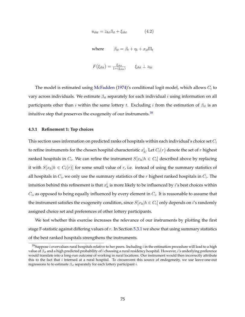
u

iht

= z

ht

�

it

+ ⇠

iht

(4.2)

where �

it

= �

t

+ ⌘

i

+ x

it

Pt

F (⇠iht

) = ⇠iht1+(⇠iht)

⇠

iht

? z

ht

The model is estimated using McFadden (1974)’s conditional logit model, which allows C

i

to

vary across individuals. We estimate �

it

separately for each individual i using information on all

participants other than i within the same lottery t. Excluding i from the estimation of �it

is an

intuitive step that preserves the exogeneity of our instruments.18

4.3.1 Refinement 1: Top choices

This section uses information on predicted ranks of hospitals within each individual’s choice set Ci

to refine instruments for the chosen hospital characteristic x

i

h

. Let Ci

(r) denote the set of r highest

ranked hospitals in C

i

. We can refine the instrument S[xh

|h 2 C

i

] described above by replacing

it with S[xh

|h 2 C

i

(r)] for some small value of r, i.e. instead of using the summary statistics of

all hospitals in C

i

, we only use the summary statistics of the r highest ranked hospitals in C

i

. The

intuition behind this refinement is that xih

is more likely to be influenced by i’s best choices within

C

i

, as opposed to being equally influenced by every element in C

i

. It is reasonable to assume that

the instrument satisfies the exogeneity condition, since S[xh

|h 2 C

i

] only depends on i’s randomly

assigned choice set and preferences of other lottery participants.

We test whether this exercise increases the relevance of our instruments by plotting the first

stage F-statistic against differing values of r. In Section 5.3.1 we show that using summary statistics

of the best ranked hospitals strengthens the instruments.

18Suppose i overvalues rural hospitals relative to her peers. Including i in the estimation procedure will lead to a highvalue of �it and a high predicted probability of i choosing a rural residency hospital. However, i’s underlying preferencewould translate into a long-run outcome of working in rural locations. Our instrument would then incorrectly attributethis to the fact that i interned at a rural hospital. To circumvent this source of endogeneity, we use leave-one-outregressions to to estimate �it separately for each lottery participant i.

75

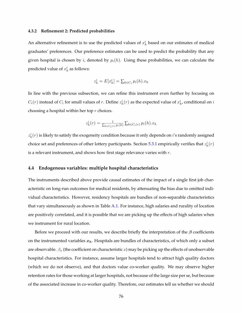
4.3.2 Refinement 2: Predicted probabilities

An alternative refinement is to use the predicted values of xih

based on our estimates of medical

graduates’ preferences. Our preference estimates can be used to predict the probability that any

given hospital is chosen by i, denoted by p

i

(h). Using these probabilities, we can calculate the

predicted value of xih

as follows:

z

i

h

= E[xih

] = Âh2Ci

p

i

(h).xh

In line with the previous subsection, we can refine this instrument even further by focusing on

C

i

(r) instead of Ci

for small values of r. Define z

i

h

(r) as the expected value of xih

, conditional on i

choosing a hospital within her top r choices.

z

i

h

(r) = 1Âh2Ci(r)

pi(h)Â

h2Ci(r) pi(h).xh

z

i

h

(r) is likely to satisfy the exogeneity condition because it only depends on i’s randomly assigned

choice set and preferences of other lottery participants. Section 5.3.1 empirically verifies that zih

(r)

is a relevant instrument, and shows how first stage relevance varies with r.

4.4 Endogenous variables: multiple hospital characteristics

The instruments described above provide causal estimates of the impact of a single first job char-

acteristic on long-run outcomes for medical residents, by attenuating the bias due to omitted indi-

vidual characteristics. However, residency hospitals are bundles of non-separable characteristics

that vary simultaneously as shown in Table A.1. For instance, high salaries and rurality of location

are positively correlated, and it is possible that we are picking up the effects of high salaries when

we instrument for rural location.

Before we proceed with our results, we describe briefly the interpretation of the � coefficients

on the instrumented variables xh. Hospitals are bundles of characteristics, of which only a subset

are observable. �x

(the coefficient on characteristic x) may be picking up the effects of unobservable

hospital characteristics. For instance, assume larger hospitals tend to attract high quality doctors

(which we do not observe), and that doctors value co-worker quality. We may observe higher

retention rates for those working at larger hospitals, not because of the large size per se, but because

of the associated increase in co-worker quality. Therefore, our estimates tell us whether we should

76

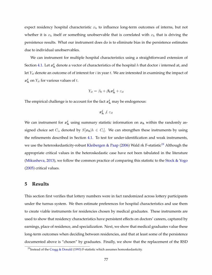
expect residency hospital characteristic x

h

to influence long-term outcomes of interns, but not

whether it is x

h

itself or something unobservable that is correlated with x

h

that is driving the

persistence results. What our instrument does do is to eliminate bias in the persistence estimates

due to individual unobservables.

We can instrument for multiple hospital characteristics using a straightforward extension of

Section 4.1. Let xih denote a vector of characteristics of the hospital h that doctor i interned at, and

let Yit

denote an outcome of of interest for i in year t. We are interested in examining the impact of

x

ih on Y

it

for various values of t.

Y

it

= �0 + �1xih + "

it

The empirical challenge is to account for the fact xih may be endogenous:

x

ih 6? "

it

We can instrument for x

ih using summary statistic information on xh within the randomly as-

signed choice set C

i

, denoted by S[xh|h 2 C

i

]. We can strengthen these instruments by using

the refinements described in Section 4.1. To test for under-identification and weak instruments,

we use the heteroskedasticity-robust Kleibergen & Paap (2006) Wald rk F-statistic19 Although the

appropriate critical values in the heteroskedastic case have not been tabulated in the literature

(Mikusheva, 2013), we follow the common practice of comparing this statistic to the Stock & Yogo

(2005) critical values.

5 Results

This section first verifies that lottery numbers were in fact randomized across lottery participants

under the turnus system. We then estimate preferences for hospital characteristics and use them

to create viable instruments for residencies chosen by medical graduates. These instruments are

used to show that residency characteristics have persistent effects on doctors’ careers, captured by

earnings, place of residence, and specialization. Next, we show that medical graduates value these

long-term outcomes when deciding between residencies, and that at least some of the persistence

documented above is “chosen” by graduates. Finally, we show that the replacement of the RSD

19Instead of the Cragg & Donald (1993) F-statistic which assumes homoskedasticity.

77

mechanism with decentralized job-finding in 2013 altered the distribution of worker welfare across

worker types, and total worker welfare.

5.1 Randomization

First, we test that the lottery was able to successfully randomize draw numbers. A formal test is

that individual characteristics ⇣i

should not affect her lottery draw number DiL

.

D

iL

= �⇣

i

+ �

L

+ "

iL

We normalize lottery draws to lie on the interval [0, 1] by dividing by the largest draw number.

We also include lottery fixed effects to account for lottery specific shocks such as larger participa-

tion overall, or larger participation by particular demographics in a given lottery. Table 3 displays

the results of regressions for five individual characteristics: rurality of hometown20, gender, age,

whether the participant was born abroad, and whether he studied abroad. None of these charac-

teristics are significant predictors of an individual’s lottery draw number.21

5.2 Doctor preferences

This section describes our estimates of lottery participants’ preferences for residency characteris-

tics. We divide interns on the basis of gender, birth country, and rurality of hometown (if born in

Norway), and estimate preferences separately for each group.22

Table A.3 displays preference estimates based on section 4.3 for the following hospital char-

acteristics: log salary,23 rural location, proportion of specialists, number of specialists in internal

medicine, surgery, diagnostic medicine and psychiatry,24 as well as hospital size (log number of

doctors). Interns across demographic groups value larger hospitals, reflected by the significant and

positive coefficient on hospital size. To enable comparisons across demographic groups, we restate

20Hometown is defined as the municipality at age 15, and rurality measures the proportion of rural residents in themunicipality.

21Results do not change meaningfully if we include all five characteristics in a single regression.22An intern’s hometown is classified as rural if, at age fifteen, he lived in a municipality in which the proportion of

people living in rural areas was above the median (which is about 10 per cent). If this information is not available, it isreplaced by rurality of the municipality at age 5 or municipality at birth. Data on municipality rurality is only availablefrom 1990 onwards, so if the year at age 0/5/15 is prior to 1990, we use the rurality of the municipality in 1990 instead.

23An estimate based on the average salary of the previous year’s interns at the same hospital.24We have included the number of specialists rather than the existence of the most popular specializations (internal,

surgery, diagnostic) since there usually exists at least one specialist in each category at any given hospital, leading tomulticollinearity problems in the regression. See Table 1.

78

intern preferences in marginal willingness to pay terms, i.e. we focus on the ratio at which interns

are willing to substitute hospital characteristics for an additional percent increase in hospital size.

These results are displayed in Table 4. As noted above, each entry displays the marginal will-

ingness to pay for a percentage point increase in hospital size. Interestingly, coefficients on resi-

dency salary are either negative (most Norwegians) or not significantly different from zero (for-

eigners and urban Norwegian men).25 As expected, Norwegians from rural municipalities do

not place a negative weight on rural locations, while the reverse is true for foreigners and urban

Norwegian women. Male doctors value specialized hospitals (relative to hospital size) more than

female doctors. Foreigners and urban Norwegians value hospitals with more surgeons and less

internal medicine specialists; rural Norwegians do not display strong preferences towards specific

specializations.

5.3 Persistent effects of residency characteristics

This section examines the long-term impact (FJEs) of eight residency characteristics: salary, rurality

of location, proportion of specialists, number of specialists in internal medicine, surgery, diagnostic

medicine and psychiatry, and hospital size (number of doctors). We instrument for residency char-

acteristics using the strategies detailed in Section 4.2 and show that FJEs on income, specialization

and location decisions of doctors can persist for up to ten years.

5.3.1 First stage

Summary statistics (mean, median, variance) of hospital characteristics in C

i

sets qualify as in-

strumental variables for residency characteristics actually chosen by i. We use the refinements

described in Section 4.2 to increase their first stage explanatory power. Motivated by the prefer-

ence patterns documented above, we sort individuals into four demographic groups: foreigners,

rural-born Norwegians, urban female Norwegians and urban male Norwegians. Each resident i’s

choices are assigned probability weights based on the choices of other residents belonging to the

same demographic group in the same lottery. We then use these probability weights in two ways.

One, we restrict attention to the top seven choices when calculating summary statistics.26 Second,25The negative coefficients on hospital salary are not economically intuitive, but may be driven by the fact that we do

not observe hours worked. Also see Agarwal (2015) for another instance in the literature.26This number is based on the restriction that gives us the most powerful instrument, as displayed in Figure A.5.

79

we create weighted summary statistics, which prioritize hospitals that are most likely to be chosen

by i.

Our first set of instruments consists of the expected values of residency characteristics, as well

as the standard deviation of average hospital salary and number of doctors.27 Figure 3 illustrates

how relevance increases when we constrain attention to higher ranks to construct instruments:

for each refinement, we plot first stage Kleibergen-Paap Wald rk statistics for the highest rank

summary statistics are constrained to.28 Instrument relevance is highest for weighted summary

statistics based on the top seven hospitals of each resident’s choice set. Appendix Figure A.5 dis-

plays weak instrument tests for alternative summary statistics like quartiles as instruments, which

deliver weaker first stages than the one outlined above. Therefore, we use expected values and

standard deviations as instruments in the analysis that follows.

5.3.2 Second stage: effects on long-run outcomes

In this section, we instrument for residency characteristics and show that they continue to influence

doctors’ careers for over ten years after the completion of their residencies.

We focus on three aspects of doctors’ careers: earnings, the decision to specialize and location.

�

2 tests are used to test whether FJEs of eight residency characteristics are collectively different

from zero. Figure 4 displays these tests for each year following the lottery. We find that FJEs on

each of these outcomes continue to be significantly different from zero for over ten years after the

residency period.29 The pattern documented in the middle panel is especially interesting. Most

doctors become specialists 8-12 years after their residencies, and the peaked pattern of �

2 tests

suggests that FJEs significantly affect the decision to specialize in fields that take less time, or

that FJEs are more significant for the decision to specialize sooner (than average) in one’s career.

Figure A.6 repeats this exercise separately for the four demographic groups described above: FJEs

continue to impact earnings and the decision to specialize well beyond ten years after residency

27This enables us to run weak instrument tests, which require the number of instruments to exceed the number ofendogenous variables (henceforth, EV) by at least two. The critical value for maximal 10 per cent bias with 1 EV and 3instruments is 9.08, 2 EV and 4 instruments is 7.56, 3 EV and 5 instruments is 6.61. Stock & Yogo (2005) do not reportcritical values for more than 3 EV - we assume that the declining trend from the above 3 numbers means that 6.61 is anupper bound for the critical value in the 4 EV 6 instrument case.

28Actual first stage statistics will vary, because both stages are jointly estimated in a 2SLS regression.29Tables A.4 - A.6 display the year-by-year effects of each hospital characteristic on post-residency hospital salary,

specialization and location.

80

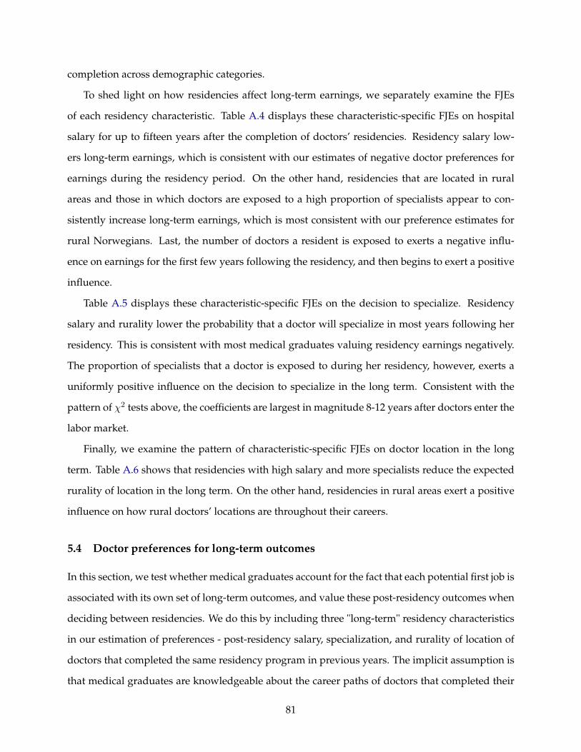
completion across demographic categories.

To shed light on how residencies affect long-term earnings, we separately examine the FJEs

of each residency characteristic. Table A.4 displays these characteristic-specific FJEs on hospital

salary for up to fifteen years after the completion of doctors’ residencies. Residency salary low-

ers long-term earnings, which is consistent with our estimates of negative doctor preferences for

earnings during the residency period. On the other hand, residencies that are located in rural

areas and those in which doctors are exposed to a high proportion of specialists appear to con-

sistently increase long-term earnings, which is most consistent with our preference estimates for

rural Norwegians. Last, the number of doctors a resident is exposed to exerts a negative influ-

ence on earnings for the first few years following the residency, and then begins to exert a positive

influence.

Table A.5 displays these characteristic-specific FJEs on the decision to specialize. Residency

salary and rurality lower the probability that a doctor will specialize in most years following her

residency. This is consistent with most medical graduates valuing residency earnings negatively.

The proportion of specialists that a doctor is exposed to during her residency, however, exerts a

uniformly positive influence on the decision to specialize in the long term. Consistent with the

pattern of �2 tests above, the coefficients are largest in magnitude 8-12 years after doctors enter the

labor market.

Finally, we examine the pattern of characteristic-specific FJEs on doctor location in the long

term. Table A.6 shows that residencies with high salary and more specialists reduce the expected

rurality of location in the long term. On the other hand, residencies in rural areas exert a positive

influence on how rural doctors’ locations are throughout their careers.

5.4 Doctor preferences for long-term outcomes

In this section, we test whether medical graduates account for the fact that each potential first job is

associated with its own set of long-term outcomes, and value these post-residency outcomes when

deciding between residencies. We do this by including three "long-term" residency characteristics

in our estimation of preferences - post-residency salary, specialization, and rurality of location of

doctors that completed the same residency program in previous years. The implicit assumption is

that medical graduates are knowledgeable about the career paths of doctors that completed their

81

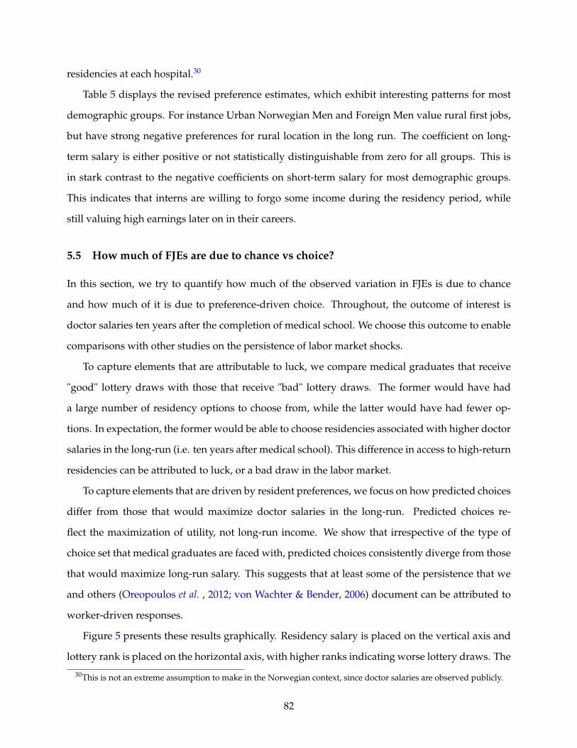
residencies at each hospital.30

Table 5 displays the revised preference estimates, which exhibit interesting patterns for most

demographic groups. For instance Urban Norwegian Men and Foreign Men value rural first jobs,

but have strong negative preferences for rural location in the long run. The coefficient on long-

term salary is either positive or not statistically distinguishable from zero for all groups. This is

in stark contrast to the negative coefficients on short-term salary for most demographic groups.

This indicates that interns are willing to forgo some income during the residency period, while

still valuing high earnings later on in their careers.

5.5 How much of FJEs are due to chance vs choice?

In this section, we try to quantify how much of the observed variation in FJEs is due to chance

and how much of it is due to preference-driven choice. Throughout, the outcome of interest is

doctor salaries ten years after the completion of medical school. We choose this outcome to enable

comparisons with other studies on the persistence of labor market shocks.

To capture elements that are attributable to luck, we compare medical graduates that receive

"good" lottery draws with those that receive "bad" lottery draws. The former would have had

a large number of residency options to choose from, while the latter would have had fewer op-

tions. In expectation, the former would be able to choose residencies associated with higher doctor

salaries in the long-run (i.e. ten years after medical school). This difference in access to high-return

residencies can be attributed to luck, or a bad draw in the labor market.

To capture elements that are driven by resident preferences, we focus on how predicted choices

differ from those that would maximize doctor salaries in the long-run. Predicted choices re-

flect the maximization of utility, not long-run income. We show that irrespective of the type of

choice set that medical graduates are faced with, predicted choices consistently diverge from those

that would maximize long-run salary. This suggests that at least some of the persistence that we

and others (Oreopoulos et al. , 2012; von Wachter & Bender, 2006) document can be attributed to

worker-driven responses.

Figure 5 presents these results graphically. Residency salary is placed on the vertical axis and

lottery rank is placed on the horizontal axis, with higher ranks indicating worse lottery draws. The

30This is not an extreme assumption to make in the Norwegian context, since doctor salaries are observed publicly.

82

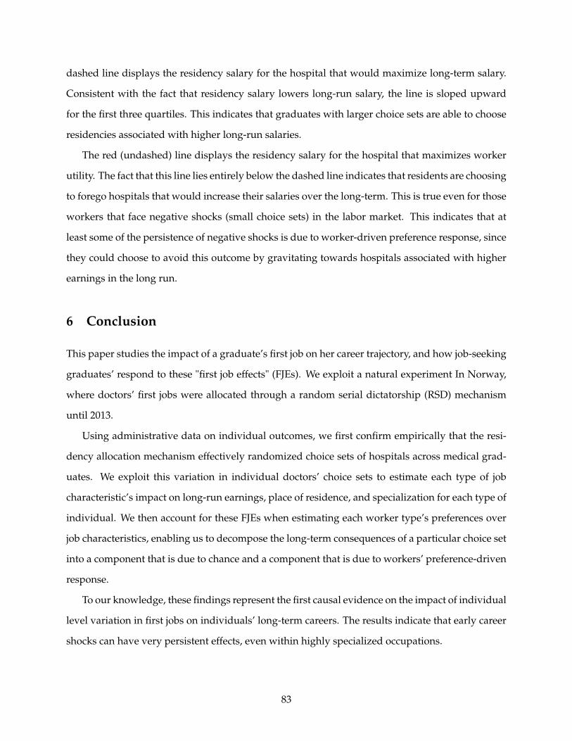
dashed line displays the residency salary for the hospital that would maximize long-term salary.

Consistent with the fact that residency salary lowers long-run salary, the line is sloped upward

for the first three quartiles. This indicates that graduates with larger choice sets are able to choose

residencies associated with higher long-run salaries.

The red (undashed) line displays the residency salary for the hospital that maximizes worker

utility. The fact that this line lies entirely below the dashed line indicates that residents are choosing

to forego hospitals that would increase their salaries over the long-term. This is true even for those

workers that face negative shocks (small choice sets) in the labor market. This indicates that at

least some of the persistence of negative shocks is due to worker-driven preference response, since

they could choose to avoid this outcome by gravitating towards hospitals associated with higher

earnings in the long run.

6 Conclusion

This paper studies the impact of a graduate’s first job on her career trajectory, and how job-seeking

graduates’ respond to these "first job effects" (FJEs). We exploit a natural experiment In Norway,

where doctors’ first jobs were allocated through a random serial dictatorship (RSD) mechanism

until 2013.

Using administrative data on individual outcomes, we first confirm empirically that the resi-

dency allocation mechanism effectively randomized choice sets of hospitals across medical grad-

uates. We exploit this variation in individual doctors’ choice sets to estimate each type of job

characteristic’s impact on long-run earnings, place of residence, and specialization for each type of

individual. We then account for these FJEs when estimating each worker type’s preferences over

job characteristics, enabling us to decompose the long-term consequences of a particular choice set

into a component that is due to chance and a component that is due to workers’ preference-driven

response.

To our knowledge, these findings represent the first causal evidence on the impact of individual

level variation in first jobs on individuals’ long-term careers. The results indicate that early career

shocks can have very persistent effects, even within highly specialized occupations.

83

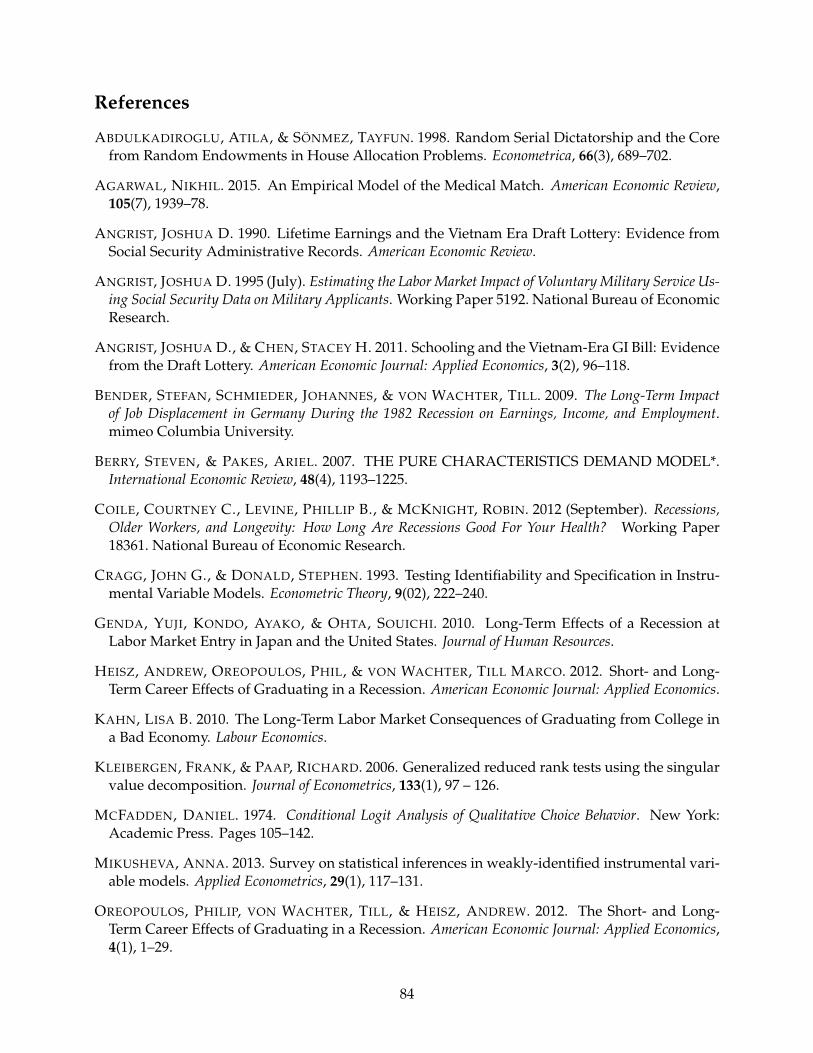
References

ABDULKADIROGLU, ATILA, & SÖNMEZ, TAYFUN. 1998. Random Serial Dictatorship and the Corefrom Random Endowments in House Allocation Problems. Econometrica, 66(3), 689–702.

AGARWAL, NIKHIL. 2015. An Empirical Model of the Medical Match. American Economic Review,105(7), 1939–78.

ANGRIST, JOSHUA D. 1990. Lifetime Earnings and the Vietnam Era Draft Lottery: Evidence fromSocial Security Administrative Records. American Economic Review.

ANGRIST, JOSHUA D. 1995 (July). Estimating the Labor Market Impact of Voluntary Military Service Us-ing Social Security Data on Military Applicants. Working Paper 5192. National Bureau of EconomicResearch.

ANGRIST, JOSHUA D., & CHEN, STACEY H. 2011. Schooling and the Vietnam-Era GI Bill: Evidencefrom the Draft Lottery. American Economic Journal: Applied Economics, 3(2), 96–118.

BENDER, STEFAN, SCHMIEDER, JOHANNES, & VON WACHTER, TILL. 2009. The Long-Term Impactof Job Displacement in Germany During the 1982 Recession on Earnings, Income, and Employment.mimeo Columbia University.

BERRY, STEVEN, & PAKES, ARIEL. 2007. THE PURE CHARACTERISTICS DEMAND MODEL*.International Economic Review, 48(4), 1193–1225.

COILE, COURTNEY C., LEVINE, PHILLIP B., & MCKNIGHT, ROBIN. 2012 (September). Recessions,Older Workers, and Longevity: How Long Are Recessions Good For Your Health? Working Paper18361. National Bureau of Economic Research.

CRAGG, JOHN G., & DONALD, STEPHEN. 1993. Testing Identifiability and Specification in Instru-mental Variable Models. Econometric Theory, 9(02), 222–240.

GENDA, YUJI, KONDO, AYAKO, & OHTA, SOUICHI. 2010. Long-Term Effects of a Recession atLabor Market Entry in Japan and the United States. Journal of Human Resources.

HEISZ, ANDREW, OREOPOULOS, PHIL, & VON WACHTER, TILL MARCO. 2012. Short- and Long-Term Career Effects of Graduating in a Recession. American Economic Journal: Applied Economics.

KAHN, LISA B. 2010. The Long-Term Labor Market Consequences of Graduating from College ina Bad Economy. Labour Economics.

KLEIBERGEN, FRANK, & PAAP, RICHARD. 2006. Generalized reduced rank tests using the singularvalue decomposition. Journal of Econometrics, 133(1), 97 – 126.

MCFADDEN, DANIEL. 1974. Conditional Logit Analysis of Qualitative Choice Behavior. New York:Academic Press. Pages 105–142.

MIKUSHEVA, ANNA. 2013. Survey on statistical inferences in weakly-identified instrumental vari-able models. Applied Econometrics, 29(1), 117–131.

OREOPOULOS, PHILIP, VON WACHTER, TILL, & HEISZ, ANDREW. 2012. The Short- and Long-Term Career Effects of Graduating in a Recession. American Economic Journal: Applied Economics,4(1), 1–29.

84

OYER, PAUL. 2006. Initial Labor Market Conditions and Long-Term Outcomes for Economists.Journal of Economic Perspectives.

OYER, PAUL. 2008. The Making of an Investment Banker: Macroeconomic Shocks, Career Choice,and Lifetime Income. Journal of Finance.

RUHM, CHRISTOPHER J. 2000. Are Recessions Good for Your Health? The Quarterly Journal ofEconomics, 115(2), 617–650.

SORKIN, ISAAC. 2016. Ranking Firms Using Revealed Preference. mimeo Stanford University.

STOCK, JAMES, & YOGO, MOTOHIRO. 2005. Testing for Weak Instruments in Linear IV Regression.New York: Cambridge University Press. Pages 80–108.

SULLIVAN, DANIEL, & VON WACHTER, TILL. 2009. Average Earnings and Long-Term Mortality:Evidence from Administrative Data. American Economic Review, 99(2), 133–38.

SULLIVAN, DANIEL, & VON WACHTER, TILL. 2009. Job Displacement and Mortality: An Analysisusing Administrative Data. Quarterly Journal of Economics.

VON WACHTER, TILL, & BENDER, STEFAN. 2006. In the Right Place at the Wrong Time: The Roleof Firms and Luck in Young Workers’ Careers. The American Economic Review, 96(5), 1679–1705.

85

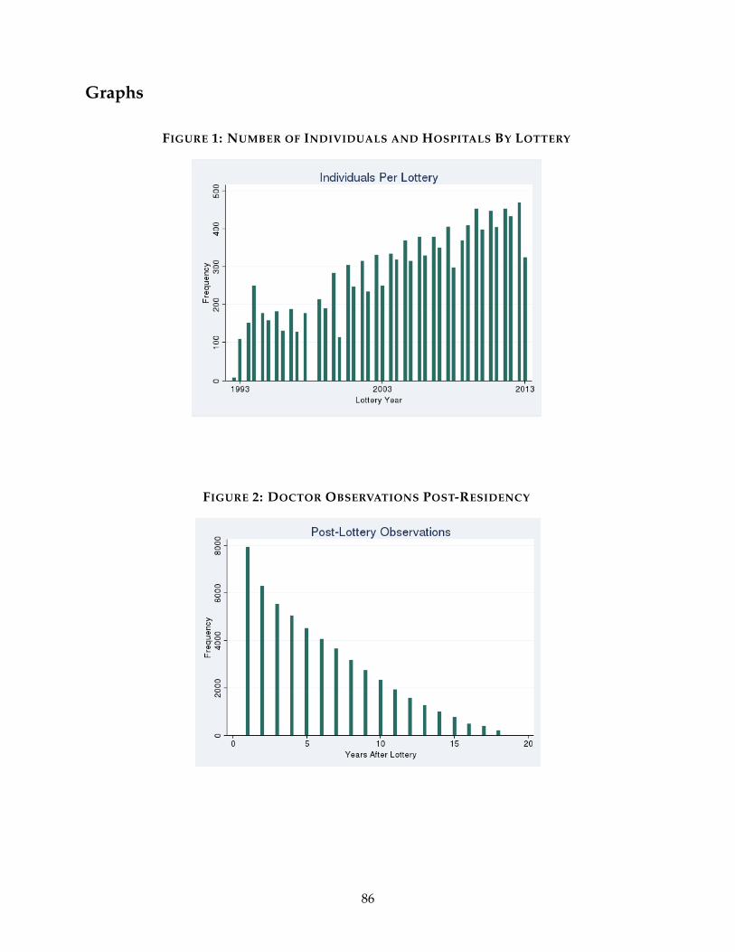
Graphs

FIGURE 1: NUMBER OF INDIVIDUALS AND HOSPITALS BY LOTTERY

FIGURE 2: DOCTOR OBSERVATIONS POST-RESIDENCY

86

FIGURE 3: FIRST STAGE REFINEMENTS

Notes: Mean and standard deviation as instruments

87

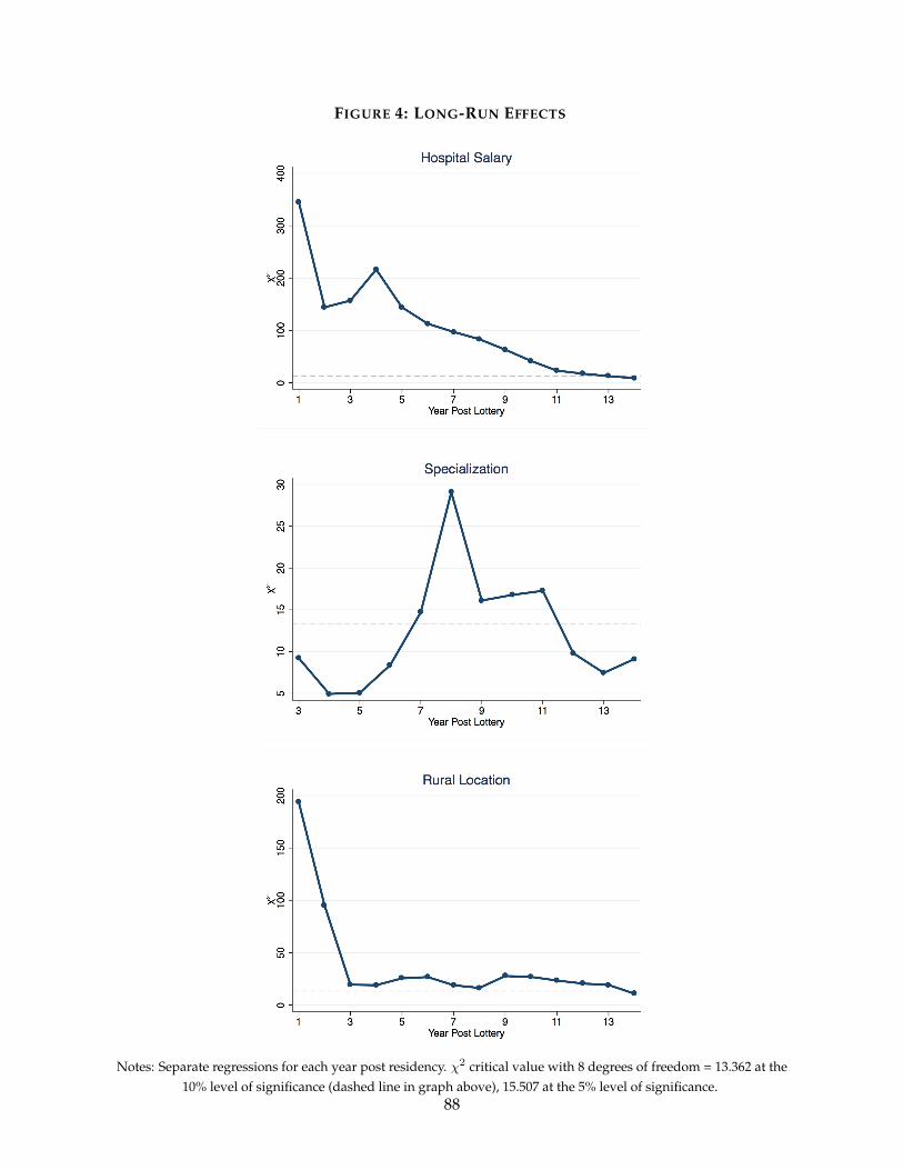
FIGURE 4: LONG-RUN EFFECTS

Notes: Separate regressions for each year post residency. �2 critical value with 8 degrees of freedom = 13.362 at the10% level of significance (dashed line in graph above), 15.507 at the 5% level of significance.

88

FIGURE 5: DECOMPOSING FJES

Notes: The dashed line plots residency salary at the hospital that would maximize doctor salary 10 years later. The redline plots residency salary at the hospital that maximizes worker utility. The horizontal axis plots quartiles for lottery

rank, with higher ranks indicating worse lottery draws and smaller choice sets.

89

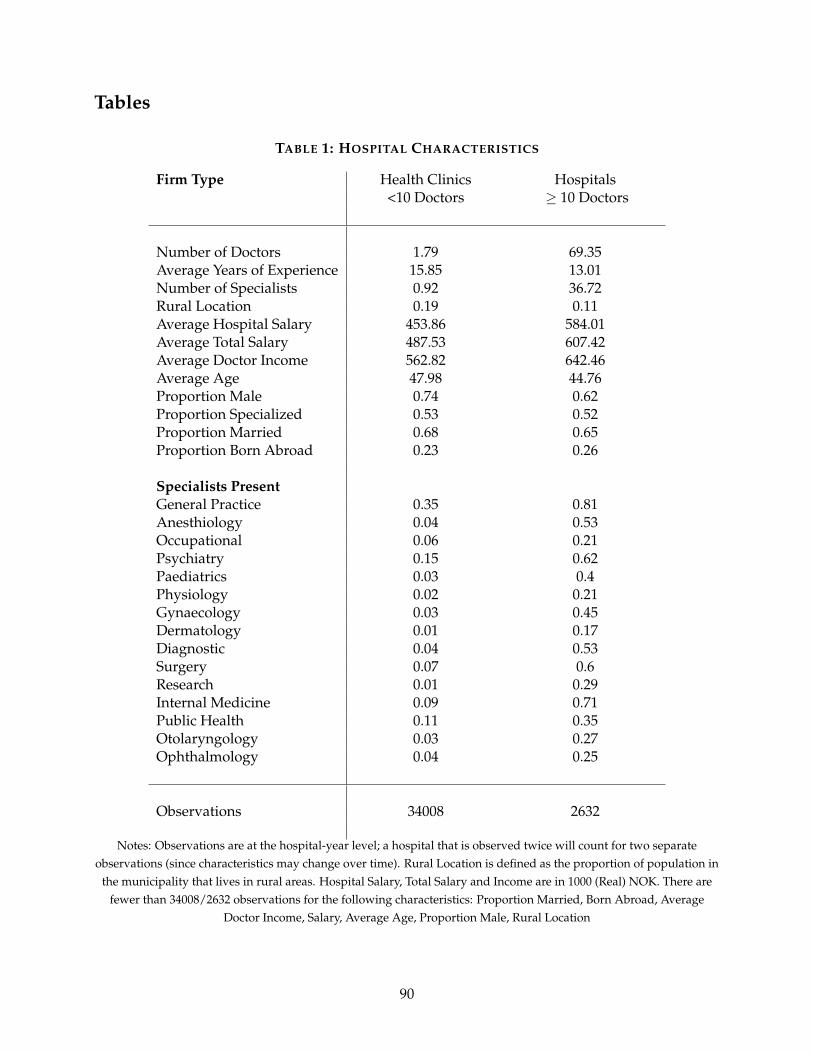
Tables

TABLE 1: HOSPITAL CHARACTERISTICS

Firm Type Health Clinics Hospitals<10 Doctors � 10 Doctors

Number of Doctors 1.79 69.35Average Years of Experience 15.85 13.01Number of Specialists 0.92 36.72Rural Location 0.19 0.11Average Hospital Salary 453.86 584.01Average Total Salary 487.53 607.42Average Doctor Income 562.82 642.46Average Age 47.98 44.76Proportion Male 0.74 0.62Proportion Specialized 0.53 0.52Proportion Married 0.68 0.65Proportion Born Abroad 0.23 0.26

Specialists PresentGeneral Practice 0.35 0.81Anesthiology 0.04 0.53Occupational 0.06 0.21Psychiatry 0.15 0.62Paediatrics 0.03 0.4Physiology 0.02 0.21Gynaecology 0.03 0.45Dermatology 0.01 0.17Diagnostic 0.04 0.53Surgery 0.07 0.6Research 0.01 0.29Internal Medicine 0.09 0.71Public Health 0.11 0.35Otolaryngology 0.03 0.27Ophthalmology 0.04 0.25

Observations 34008 2632

Notes: Observations are at the hospital-year level; a hospital that is observed twice will count for two separateobservations (since characteristics may change over time). Rural Location is defined as the proportion of population in

the municipality that lives in rural areas. Hospital Salary, Total Salary and Income are in 1000 (Real) NOK. There arefewer than 34008/2632 observations for the following characteristics: Proportion Married, Born Abroad, Average

Doctor Income, Salary, Average Age, Proportion Male, Rural Location

90

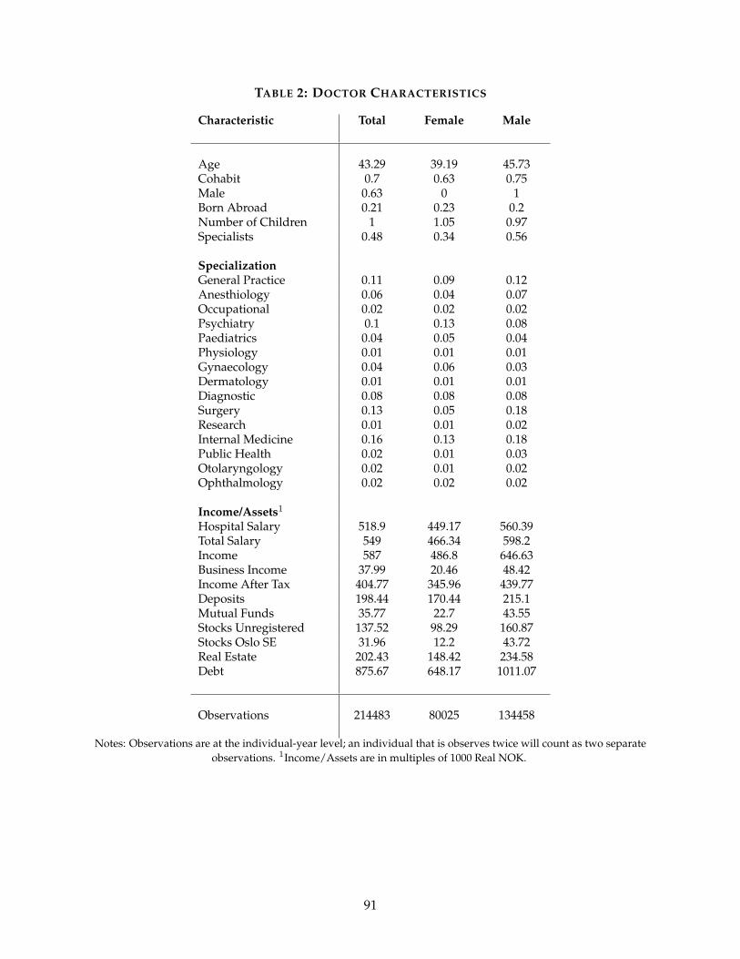
TABLE 2: DOCTOR CHARACTERISTICS

Characteristic Total Female Male

Age 43.29 39.19 45.73Cohabit 0.7 0.63 0.75Male 0.63 0 1Born Abroad 0.21 0.23 0.2Number of Children 1 1.05 0.97Specialists 0.48 0.34 0.56

SpecializationGeneral Practice 0.11 0.09 0.12Anesthiology 0.06 0.04 0.07Occupational 0.02 0.02 0.02Psychiatry 0.1 0.13 0.08Paediatrics 0.04 0.05 0.04Physiology 0.01 0.01 0.01Gynaecology 0.04 0.06 0.03Dermatology 0.01 0.01 0.01Diagnostic 0.08 0.08 0.08Surgery 0.13 0.05 0.18Research 0.01 0.01 0.02Internal Medicine 0.16 0.13 0.18Public Health 0.02 0.01 0.03Otolaryngology 0.02 0.01 0.02Ophthalmology 0.02 0.02 0.02

Income/Assets1

Hospital Salary 518.9 449.17 560.39Total Salary 549 466.34 598.2Income 587 486.8 646.63Business Income 37.99 20.46 48.42Income After Tax 404.77 345.96 439.77Deposits 198.44 170.44 215.1Mutual Funds 35.77 22.7 43.55Stocks Unregistered 137.52 98.29 160.87Stocks Oslo SE 31.96 12.2 43.72Real Estate 202.43 148.42 234.58Debt 875.67 648.17 1011.07

Observations 214483 80025 134458

Notes: Observations are at the individual-year level; an individual that is observes twice will count as two separateobservations. 1Income/Assets are in multiples of 1000 Real NOK.

91

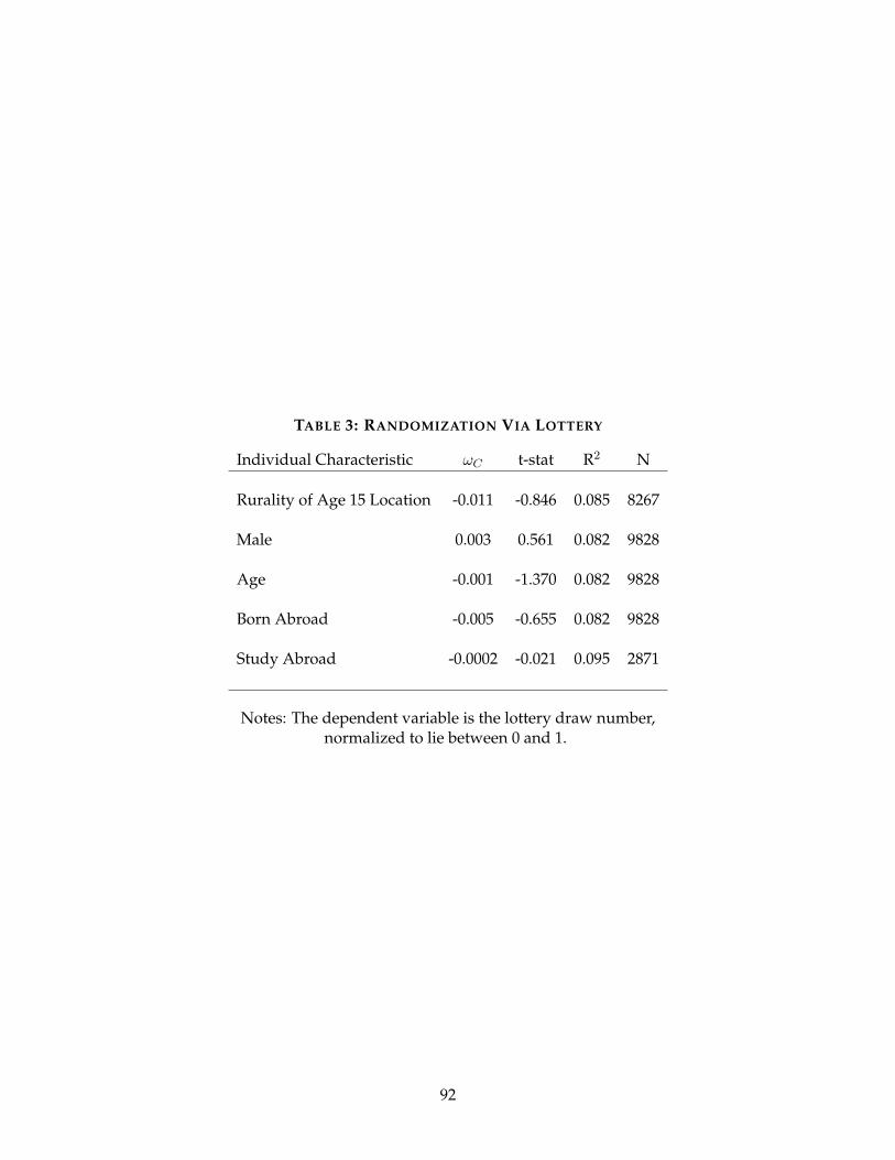
TABLE 3: RANDOMIZATION VIA LOTTERY

Individual Characteristic !

C

t-stat R2 N

Rurality of Age 15 Location -0.011 -0.846 0.085 8267

Male 0.003 0.561 0.082 9828

Age -0.001 -1.370 0.082 9828

Born Abroad -0.005 -0.655 0.082 9828

Study Abroad -0.0002 -0.021 0.095 2871

Notes: The dependent variable is the lottery draw number,normalized to lie between 0 and 1.

92

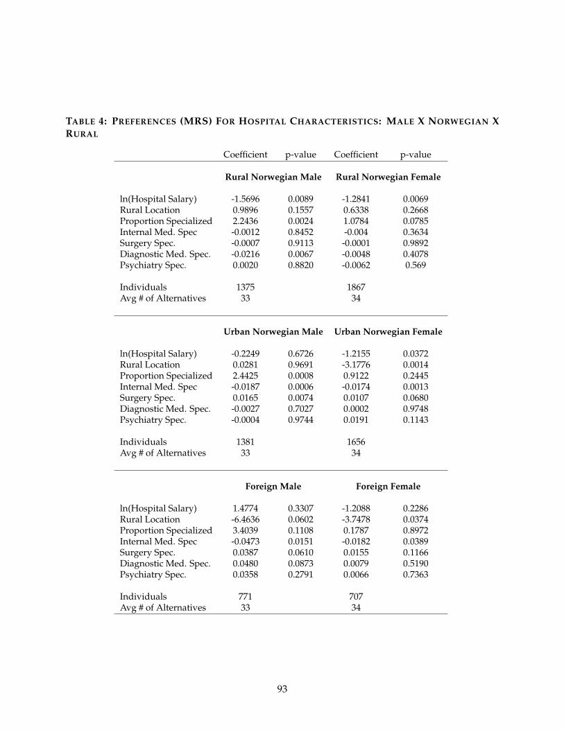
TABLE 4: PREFERENCES (MRS) FOR HOSPITAL CHARACTERISTICS: MALE X NORWEGIAN XRURAL

Coefficient p-value Coefficient p-value

Rural Norwegian Male Rural Norwegian Female

ln(Hospital Salary) -1.5696 0.0089 -1.2841 0.0069Rural Location 0.9896 0.1557 0.6338 0.2668Proportion Specialized 2.2436 0.0024 1.0784 0.0785Internal Med. Spec -0.0012 0.8452 -0.004 0.3634Surgery Spec. -0.0007 0.9113 -0.0001 0.9892Diagnostic Med. Spec. -0.0216 0.0067 -0.0048 0.4078Psychiatry Spec. 0.0020 0.8820 -0.0062 0.569

Individuals 1375 1867Avg # of Alternatives 33 34

Urban Norwegian Male Urban Norwegian Female

ln(Hospital Salary) -0.2249 0.6726 -1.2155 0.0372Rural Location 0.0281 0.9691 -3.1776 0.0014Proportion Specialized 2.4425 0.0008 0.9122 0.2445Internal Med. Spec -0.0187 0.0006 -0.0174 0.0013Surgery Spec. 0.0165 0.0074 0.0107 0.0680Diagnostic Med. Spec. -0.0027 0.7027 0.0002 0.9748Psychiatry Spec. -0.0004 0.9744 0.0191 0.1143

Individuals 1381 1656Avg # of Alternatives 33 34

Foreign Male Foreign Female

ln(Hospital Salary) 1.4774 0.3307 -1.2088 0.2286Rural Location -6.4636 0.0602 -3.7478 0.0374Proportion Specialized 3.4039 0.1108 0.1787 0.8972Internal Med. Spec -0.0473 0.0151 -0.0182 0.0389Surgery Spec. 0.0387 0.0610 0.0155 0.1166Diagnostic Med. Spec. 0.0480 0.0873 0.0079 0.5190Psychiatry Spec. 0.0358 0.2791 0.0066 0.7363

Individuals 771 707Avg # of Alternatives 33 34

93

TABLE 5: PREFERENCES (MRS) FOR LONG-TERM HOSPITAL CHARACTERISTICS

Coefficient p-value Coefficient p-value

Rural Norwegian Male Rural Norwegian Female

ln(Long-Term Hospital Salary) 0.5163 0.5713 -1.0179 0.1418Long-Term Rurality 4.8327 0.0201 -1.1661 0.4766Long-Term Specialization 9.0542 0.0103 5.7596 0.0269ln(Hospital Salary) -1.8134 0.0083 -1.3349 0.0123Rural Location -0.8001 0.4764 1.1057 0.1891Proportion Specialized 2.0324 0.0144 0.8268 0.2289Internal Med. Spec -0.0022 0.7228 -0.0019 0.6862Surgery Spec. 0.0037 0.5912 -0.0005 0.9214Diagnostic Med. Spec. -0.0215 0.008 -0.0084 0.1555Psychiatry Spec. -0.0041 0.7823 -0.0172 0.1542

Individuals 1207 1695Avg # of Alternatives 33 34

Urban Norwegian Male Urban Norwegian Female

ln(Long-Term Hospital Salary) -0.8236 0.3183 -1.1268 0.1464Long-Term Rurality -12.3673 0 -10.6118 0Long-Term Specialization -2.1823 0.4693 1.474 0.5778ln(Hospital Salary) -0.2561 0.672 -1.1581 0.0488Rural Location 4.3765 0 1.3201 0.158Proportion Specialized 2.4839 0.0034 0.5209 0.519Internal Med. Spec -0.0151 0.0066 -0.0142 0.0041Surgery Spec. 0.0112 0.0811 0.0063 0.2529Diagnostic Med. Spec. -0.005 0.492 -0.0029 0.6549Psychiatry Spec. -0.0132 0.398 0.0113 0.346

Individuals 1236 1519Avg # of Alternatives 33 34

Foreign Male Foreign Female

ln(Long-Term Hospital Salary) -2.7853 0.1788 1.3425 0.4081Long-Term Rurality -24.9915 0.0075 -12.7774 0.0084Long-Term Specialization -5.3944 0.499 1.1741 0.83ln(Hospital Salary) -0.3845 0.7987 -1.9329 0.1117Rural Location 4.0115 0.1109 -0.1236 0.9502Proportion Specialized 1.582 0.4376 -0.487 0.757Internal Med. Spec -0.0236 0.1138 -0.0208 0.0341Surgery Spec. 0.0138 0.3956 0.0186 0.1074Diagnostic Med. Spec. 0.0291 0.2022 0.0082 0.5404Psychiatry Spec. -0.0402 0.3199 0.0136 0.5249

Individuals 702 670Avg # of Alternatives 33 34

94

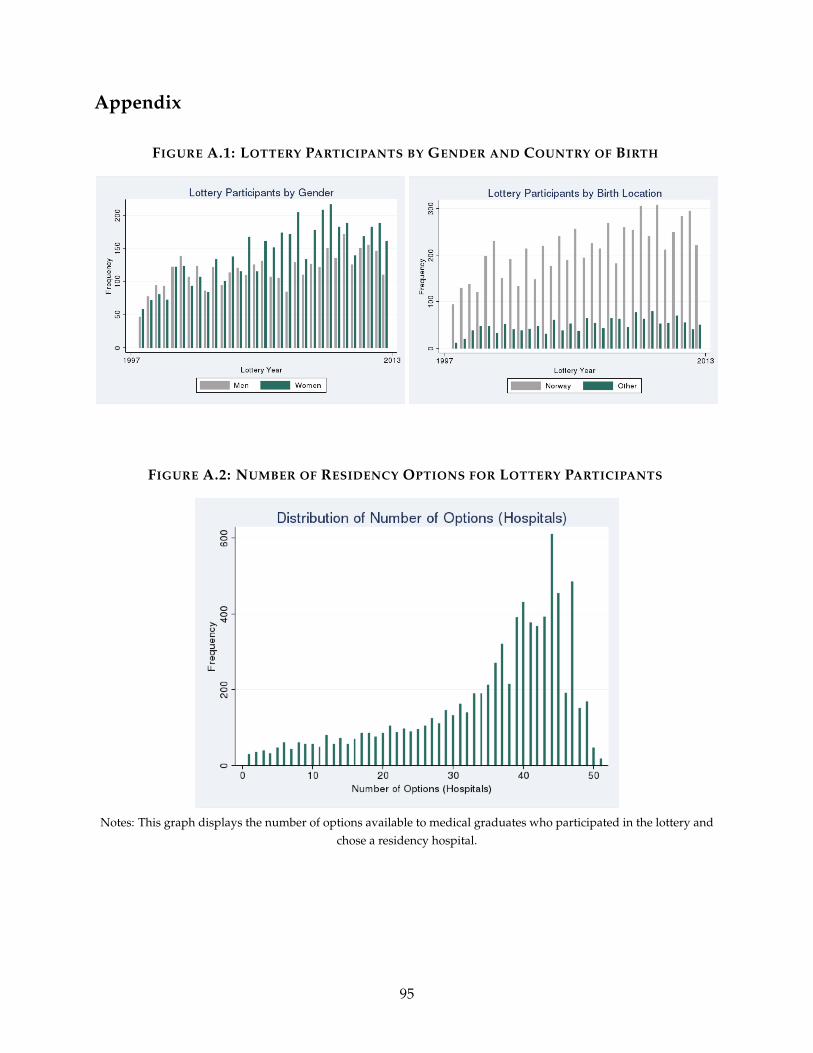
Appendix

FIGURE A.1: LOTTERY PARTICIPANTS BY GENDER AND COUNTRY OF BIRTH

FIGURE A.2: NUMBER OF RESIDENCY OPTIONS FOR LOTTERY PARTICIPANTS

Notes: This graph displays the number of options available to medical graduates who participated in the lottery andchose a residency hospital.

95

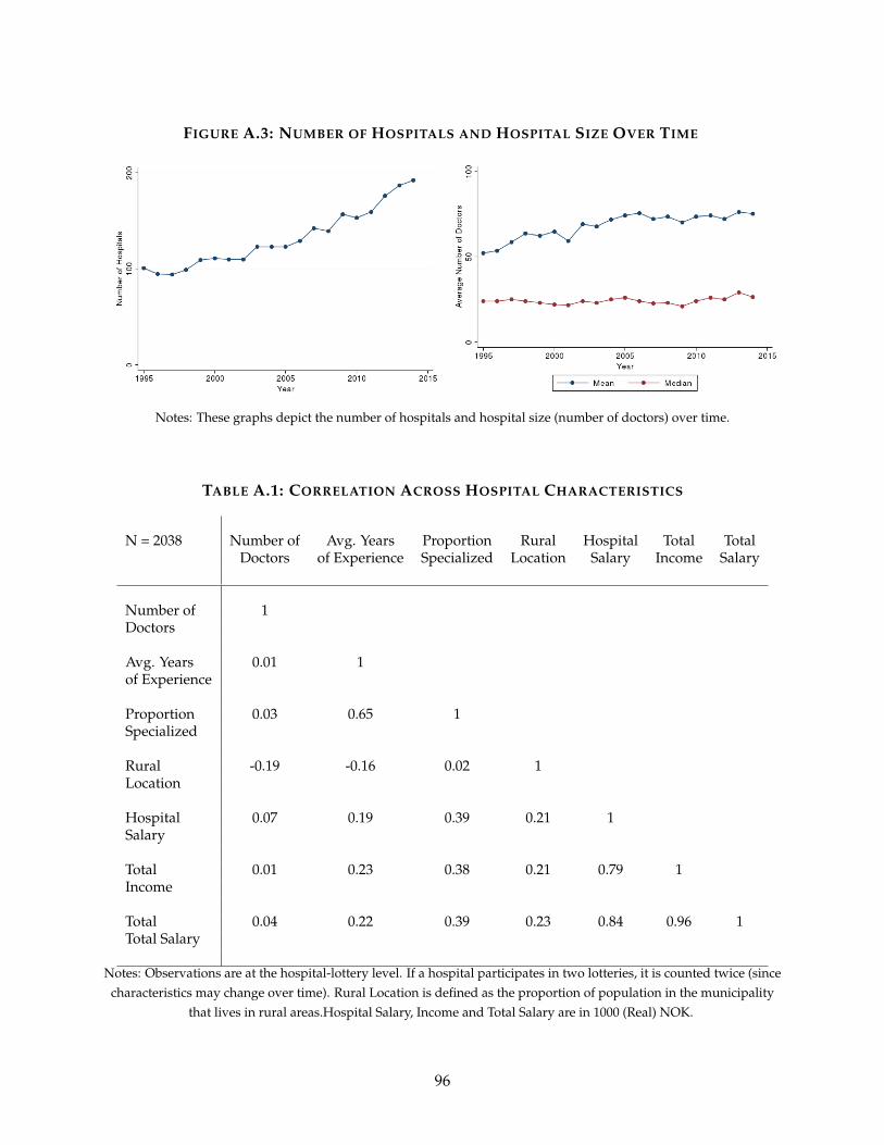
FIGURE A.3: NUMBER OF HOSPITALS AND HOSPITAL SIZE OVER TIME

Notes: These graphs depict the number of hospitals and hospital size (number of doctors) over time.

TABLE A.1: CORRELATION ACROSS HOSPITAL CHARACTERISTICS

N = 2038 Number of Avg. Years Proportion Rural Hospital Total TotalDoctors of Experience Specialized Location Salary Income Salary

Number of 1Doctors

Avg. Years 0.01 1of Experience

Proportion 0.03 0.65 1Specialized

Rural -0.19 -0.16 0.02 1Location

Hospital 0.07 0.19 0.39 0.21 1Salary

Total 0.01 0.23 0.38 0.21 0.79 1Income

Total 0.04 0.22 0.39 0.23 0.84 0.96 1Total Salary

Notes: Observations are at the hospital-lottery level. If a hospital participates in two lotteries, it is counted twice (sincecharacteristics may change over time). Rural Location is defined as the proportion of population in the municipality

that lives in rural areas.Hospital Salary, Income and Total Salary are in 1000 (Real) NOK.

96

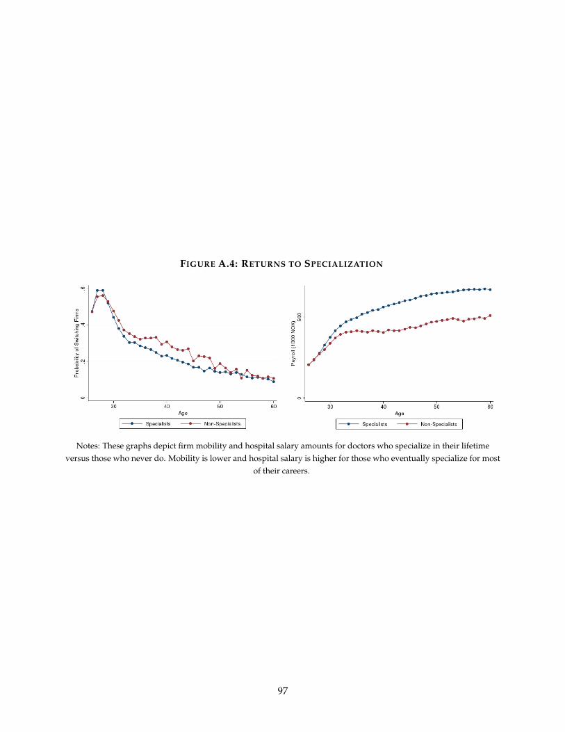
FIGURE A.4: RETURNS TO SPECIALIZATION

Notes: These graphs depict firm mobility and hospital salary amounts for doctors who specialize in their lifetimeversus those who never do. Mobility is lower and hospital salary is higher for those who eventually specialize for most

of their careers.

97

FIGURE A.5: ALTERNATIVE FIRST STAGE REFINEMENTS

(a) 25th, 50th and 75th Percentiles as Instruments

(b) Mean, 1st and 99th Percentiles as Instruments

98

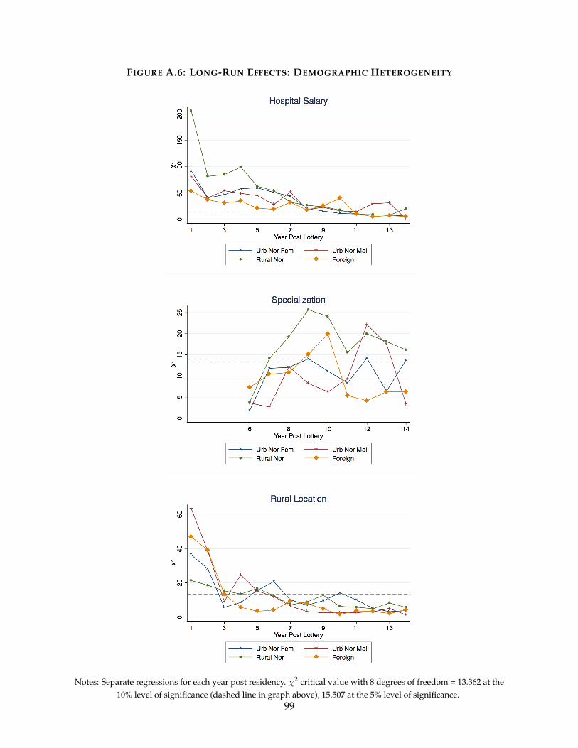
FIGURE A.6: LONG-RUN EFFECTS: DEMOGRAPHIC HETEROGENEITY

Notes: Separate regressions for each year post residency. �2 critical value with 8 degrees of freedom = 13.362 at the10% level of significance (dashed line in graph above), 15.507 at the 5% level of significance.

99

TABLE A.2: SALARY VARIATION WITH FIRM AND INDIVIDUAL CHARACTERISTICS

Characteristic Coefficient CoefficientDoctors 2-3 70.46 72.64

(2.94) (2.88)Doctors 4-9 114.13 106.43

(2.6) (2.61)Doctors � 10 184.84 139.54

(2.06) (2.16)Average Years of Experience -3.56 -4.04

(0.15) (0.15)Proportion Specialized 49.62 101.9

(3.66) (3.46)Rural Location 5.13 44.43

(3.58) (3.56)Male 69.4 60.71

(0.94) (0.93)Born Abroad -0.88 -9.76

(1.14) (1.11)Specialist 107.18

(1.44)General Practice -57.98

(1.68)Anesthiology 151.17

(2.31)Occupational 38.47

(3.25)Psychiatry 64.87

(1.64)Paediatrics 65.5

(2.17)Physiology 8.59

(3.68)Gynaecology 118.7

(2.45)Dermatology 26.76

(5.75)Diagnostic 113.35

(1.99)Surgery 152.85

(1.67)Research 27.61

(4.16)Internal Medicine 48.33

(1.34)Public Health 9.49

(2.91)Otolaryngology 70.98

(3.44)Ophthalmology 51.98

(3.29)Observations 207092 207092R2 0.39 0.42Time F.E. ⇥ ⇥Age F.E. ⇥ ⇥

Notes: Robust standard errors in parentheses.

100

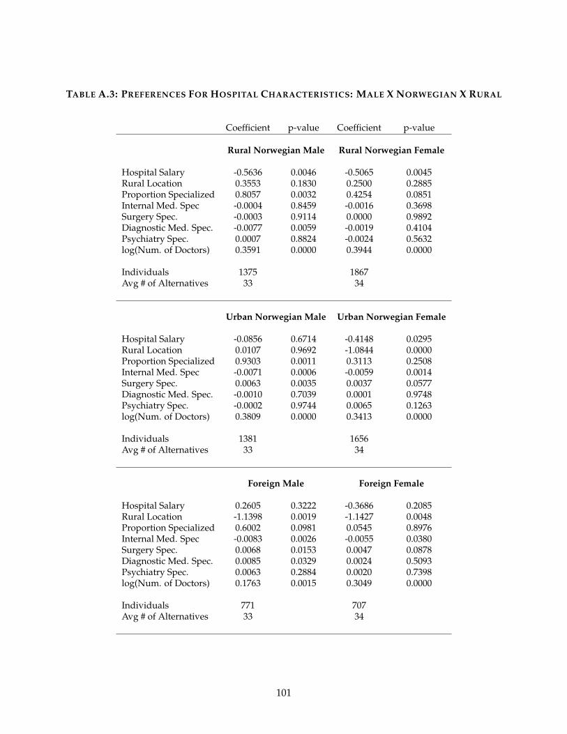
TABLE A.3: PREFERENCES FOR HOSPITAL CHARACTERISTICS: MALE X NORWEGIAN X RURAL

Coefficient p-value Coefficient p-value

Rural Norwegian Male Rural Norwegian Female

Hospital Salary -0.5636 0.0046 -0.5065 0.0045Rural Location 0.3553 0.1830 0.2500 0.2885Proportion Specialized 0.8057 0.0032 0.4254 0.0851Internal Med. Spec -0.0004 0.8459 -0.0016 0.3698Surgery Spec. -0.0003 0.9114 0.0000 0.9892Diagnostic Med. Spec. -0.0077 0.0059 -0.0019 0.4104Psychiatry Spec. 0.0007 0.8824 -0.0024 0.5632log(Num. of Doctors) 0.3591 0.0000 0.3944 0.0000

Individuals 1375 1867Avg # of Alternatives 33 34

Urban Norwegian Male Urban Norwegian Female

Hospital Salary -0.0856 0.6714 -0.4148 0.0295Rural Location 0.0107 0.9692 -1.0844 0.0000Proportion Specialized 0.9303 0.0011 0.3113 0.2508Internal Med. Spec -0.0071 0.0006 -0.0059 0.0014Surgery Spec. 0.0063 0.0035 0.0037 0.0577Diagnostic Med. Spec. -0.0010 0.7039 0.0001 0.9748Psychiatry Spec. -0.0002 0.9744 0.0065 0.1263log(Num. of Doctors) 0.3809 0.0000 0.3413 0.0000

Individuals 1381 1656Avg # of Alternatives 33 34

Foreign Male Foreign Female

Hospital Salary 0.2605 0.3222 -0.3686 0.2085Rural Location -1.1398 0.0019 -1.1427 0.0048Proportion Specialized 0.6002 0.0981 0.0545 0.8976Internal Med. Spec -0.0083 0.0026 -0.0055 0.0380Surgery Spec. 0.0068 0.0153 0.0047 0.0878Diagnostic Med. Spec. 0.0085 0.0329 0.0024 0.5093Psychiatry Spec. 0.0063 0.2884 0.0020 0.7398log(Num. of Doctors) 0.1763 0.0015 0.3049 0.0000

Individuals 771 707Avg # of Alternatives 33 34

101

TABLE A.4: LONG-TERM HOSPITAL SALARY

Year <2 2-3 4-5 6-7 8-9 10-11 12-13 14-15

Residency Salary 0.021 -0.027 0.036 -0.136 -0.185 -0.257 -0.328 -0.677(0.036) (0.063) (0.050) (0.074) (0.084) (0.106) (0.135) (0.267)

Residency Rurality -0.027 -0.767 1.227 2.795 0.232 3.495 0.603 4.858(0.629) (1.370) (1.335) (1.436) (1.398) (1.877) (2.291) (4.989)

Residency Proportion 0.153 2.803 0.196 1.620 2.619 1.928 3.198 5.482of Specialists (0.549) (0.818) (0.712) (0.889) (1.181) (1.463) (1.695) (3.206)

Residency Hospital Size 0.019 -0.216 -0.379 -1E-4 0.269 0.442 0.633 1.914(0.094) (0.176) (0.199) (0.240) (0.271) (0.334) (0.475) (0.947)

Observations 15,280 11,681 9,450 7,617 5,836 4,190 2,802 1,707Mean 2.999 4.794 6.121 6.537 7.132 7.791 8.543 9.083

102

TABLE A.5: LONG-TERMSPECIALIZATION

Year <2 2-3 4-5 6-7 8-9 10-11 12-13 14-15

Residency Salary 4E-5 -1E-5 -0.001 1E-4 -0.021 -0.043 -0.037 -0.021(0) (0.001) (0.001) (0.006) (0.013) (0.018) (0.023) (0.028)

Residency Rurality -0.004 -0.009 0.028 -0.216 -0.375 0.243 -0.008 -0.021(0.002) (0.012) (0.035) (0.119) (0.240) (0.427) (0.454) (0.584)

Residency Proportion 4E-4 -0.005 0.028 0.194 0.577 0.599 0.436 0.338of Specialists (0.002) (0.008) (0.022) (0.086) (0.212) (0.246) (0.288) (0.344)

Residency Hospital Size 1E-4 0.001 -0.002 -0.031 -0.018 0.074 0.075 0.0128(0.001) (0.002) (0.006) (0.019) (0.046) (0.056) (0.080) (0.102)

Observations 15,280 11,681 9,450 7,617 5,836 4,190 2,802 1,707Mean 0.001 0.002 0.004 0.051 0.254 0.488 0.671 0.778

103

TABLE A.6: LONG-TERM RURAL LOCATION

Year <2 2-3 4-5 6-7 8-9 10-11 12-13 14-15

Residency Salary -0.028 -0.001 -0.016 -0.011 -0.007 -0.007 -0.008 -0.010(0.005) (0.009) (0.004) (0.005) (0.005) (0.005) (0.005) (0.009)

Residency Rurality 0.907 0.453 0.461 0.317 0.228 0.355 0.293 0.752(0.115) (0.148) (0.111) (0.082) (0.080) (0.096) (0.110) (0.256)

Residency Proportion -0.223 -0.265 -0.110 -0.096 -0.101 -0.176 -0.136 -0.253of Specialists (0.090) (0.123) (0.049) (0.060) (0.057) (0.061) (0.062) (0.109)

Residency Hospital Size 0.063 0.015 0.050 0.034 0.019 0.013 0.011 -0.020(0.014) (0.020) (0.012) (0.018) (0.018) (0.014) (0.018) (0.033)

Observations 15,207 11,638 9,414 7,592 5,820 4,177 2,797 1,707Mean 0.135 0.142 0.098 0.090 0.085 0.080 0.079 0.086

104

Chapter 3

Election by Community Consensus:

Effects on Political Selection and Governance⇤

Ashna Arora†

Abstract

This paper evaluates the effects of encouraging the selection of local politicians in India

via community-based consensus, as opposed to a secret ballot election. While secret ballot

elections prevent vote capture by guaranteeing voter anonymity, consensus-based elections

may improve welfare by promoting the exchange of information. I find that incentives for

consensus-based elections crowd in politicians that are younger and more educated, but lead

to worse governance as measured by a fall in local expenditure and regressive targeting of

workfare employment. These results are consistent with qualitative evidence that finds that

community-based processes are prone to capture by the local elite, and need not improve the

quality of elected politicians or governance.

⇤I am deeply grateful to Francois Gerard, Suresh Naidu and Bernard Salanié for guidance and support. For helpful

discussions, I would like to thank Siddharth Hari, Nandita Krishnaswamy, Daniel Rappoport, Christoph Rothe and

numerous participants at the Applied Microeconomics and Development Colloquia at Columbia University as well as

the Conference on Economic Growth and Development at the Indian Statistical Institute. I also thank Kunjal Desai for

help with data access. This research was supported by the Wueller Pre-Dissertation Award at Columbia University. All

errors are my own.†Department of Economics, Columbia University. Email: aa3332@columbia.edu

105

1 Introduction

Since the 1990s, developing countries have undertaken a broad range of decentralization reforms,

aimed at enhancing the role of local stakeholders in policy making and program implementation

(Bardhan 2002). These reforms have led to the creation of democratic governments at the local

level, as well as the devolution of authority to existing local governments. In the last decade, re-

search and policy attention has shifted to deepening democratic processes within these institutions

by limiting the influence of elites and enhancing community participation in local decision mak-

ing. These policies include the use of community monitoring (Olken 2007), community meetings

(Besley et al. 2005, Rao & Ibáñez 2005, Alatas et al. 2013) and direct democracy (Olken 2008, Beath

et al. 2013, Hinnerich & Pettersson-Lidbom 2014) to implement programs based on the consensus

of local stakeholders.

This paper examines the effects of promoting community consensus as a tool to select political

representatives themselves, rather than as a tool to monitor or alter policy decisions after politi-

cians have assumed office. I first test for changes in observable politician characteristics, such as

age and education, to understand whether the policy hurts incumbents and to quantify its impact

on political selection. I also examine changes in measurable aspects of governance at the village

level, such as the amount of local expenditure and targeting of workfare employment. These out-

comes are directly affected by local politicians and can, therefore, be used to estimate the impact

of the policy on governance.

I find that promoting consensus-based elections significantly influence who communities elect,

and their performance once in office. Incentives for consensus-based elections crowd younger,

more educated representatives into political office. However, these elections also lead to a reduc-

tion in government size, reflected in a reduction in total expenditure, and more regressive target-

ing of workfare employment by the local council.1 These findings are indicative of worse gover-

nance, since development expenditure and workfare employment disproportionately benefit the

poorest households in Indian villages (Imbert & Papp 2015). Overall, the results are consistent

1Regressivity is measured by the proportion of workfare employment allocated to historically marginalized sectionsof the population.

106

with qualitative evidence that finds that community-based processes in general, and consensus-

based elections in specific, are prone to elite capture and can lead to worse governance.

To estimate the impact of encouraging consensus-based elections, I compile a new dataset con-

taining detailed information on candidates, politicians and governance indicators at the village

level in Gujarat, a state in Western India, for the years 2011-15. While many states in India in-

centivize consensus-based elections at the village level, Gujarat offers untied financial grants that

increase discontinuously with village population. In the 2011 elections in Gujarat, villages with

populations greater than 5000 faced substantially larger incentives for elections via community

consensus - the financial grant increased by fifty percent at the threshold, from 13 to 20 per cent

of the median village budget. This increase in financial incentives is used to set up a regression

discontinuity design, which tests for the causal impact of incentivizing consensus elections on po-

litical selection and governance. The identifying assumption is that unobservables vary smoothly

around this population threshold.

This setting also allows me to circumvent the contamination of estimates by multiple treat-

ments, a common drawback of regression discontinuity designs. Two features of the local political

system increase at the population threshold of 5000 - the consensus election grant and the number

of political representatives. However, the number of political representatives also increases dis-

continuously at population thresholds other than 5000. Estimates at these alternative thresholds

are used to show that this contaminating treatment (increase in the number of council members)

does not drive the findings on electoral competition, politician identity and governance.

Why would crowding in younger, more educated politicians worsen governance? The state

government does not place any restrictions on how village communities reach a consensus about

their political representatives. Survey evidence indicates that local elites usually nominate candi-

dates and mobilize support for their election by consensus, i.e., without formal opposition (Bre-

man 2011). If these candidates are inexperienced and merely serve as political placeholders, they

may lack both the ability and motivation to undertake administrative and development expendi-

tures within the village, and negotiate with bureaucrats outside the village to influence funding

107

towards workfare employment.2 Financial incentives for consensus-based elections could, there-

fore, worsen governance by crowding in politicians that rely on the support of a handful of local

elites instead of all village residents.

This paper contributes to the growing literature on the impact of electoral institutions on polit-

ical selection and governance outcomes (Diermeier et al. 2005, Keane & Merlo 2010, Banerjee et al.

2011, Banerjee et al. 2017). The results are also consistent with theoretical work that shows that

political competition and community participation may have negative or positive effects (Khwaja

2004, Caselli & Morelli 2004, Lizzeri & Persico 2005, Mattozzi & Merlo 2008). Empirical work

shows that reducing political competition can worsen legislator quality and performance (Brazil,

Ferraz & Finan 2009) and is associated with anti-growth policies (United States, Besley et al. 2010).

This paper finds broadly similar results in the Indian village setting - incentives for consensus-

based elections lower competition and crowd in younger (albeit more educated) politicians, and

reduce expenditure and worsen employment targeting by the local government.

Additionally, I find support for the citizen-candidate models of Osborne & Slivinski (1996)

and Besley & Coate (1997), which highlight the influence of politician identity on governance out-

comes. My results add to the extensive literature documenting the influence of visible politician

characteristics on governance outcomes in India (Pande 2003, Chattopadhyay & Duflo 2004, Ra-

jaraman & Gupta 2012, Afridi et al. 2013) and other countries (Powley 2007, Washington 2008).

This paper also contributes to the debate on the effects of elite influence on governance and

social welfare. Studies show that elite capture can have sizable negative consequences in some

contexts (Besley et al. 2004, Acemoglu & Robinson 2008, Caeyers & Dercon 2012, Acemoglu

et al. 2014), but that these effects may be small or completely absent in other settings (Bardhan

& Mookherjee 2006, Alatas et al. 2013, Beath et al. 2013).3 This paper concurs with the findings of

the former set of papers by showing that at least in the short term, elite influence in elections can

influence politician identity and substantially worsen governance.

Finally, these results add to the burgeoning literature on regression-discontinuity designs in

2Political and administrative inexperience has been shown to be an important determinant of implementation inef-ficiencies and leakages in the Indian village setting (Afridi et al. 2013)

3Baland & Robinson (2012) show that the introduction of the secret ballot reduced elite influence over voting deci-sions, but do not measure its impact on government performance.

108

political economics (Lee 2008, Ferraz & Finan 2009, Pettersson-Lidbom 2012, Hinnerich & Pettersson-

Lidbom 2014).

The remainder of this paper is organized into four sections. Section 2 describes the institutional

setting and the data sources. Section 3 details the empirical strategy and Section 4 presents the

results. Section 5 concludes.

2 Setting and Data

This section provides detailed information about the functioning of village governments in Gu-

jarat, the implementation of the Samras (consensus) Panchayat scheme, as well as the datasets

used in the empirical analysis.

Institutional Background

The Seventy Third Amendment to the Indian Constitution in 1992 mandated the creation of a

three tiered local government system, at the district, block and village level (in descending order

of size of jurisdiction) across states in India. This study focuses on elected councils at the village

level, also called Gram Panchayats (henceforth, GPs) in Gujarat. GP members are directly elected

for five-year terms by village residents and elections are not fought on party lines, i.e. candidates

are not affiliated with political parties at the state or national level. The jurisdiction of each GP

is divided into a number of mutually exclusive wards, and efforts are undertaken to ensure that

each ward contains the same number of residents. The population of each ward then elects a

single representative to occupy a GP seat. In Gujarat, the number of ward members is fixed at

7 for GPs with populations up to 3000, and increases by 2 for every multiple of 1000 thereafter.

Figure 1 uses electoral data to plot the actual number of GP members elected in the 2011 elections

against GP population in Gujarat, and shows that this rule was closely followed in practice. The

village community as a whole also directly elects the president of the GP.

The Seventy Third Constitutional Amendment also mandated reservations for women, and

three disadvantaged classes - Scheduled Castes, Scheduled Tribes and Other Backward Classes

109

at the district, block and village level.4 At least 33 per cent of president and council member

seats are reserved for women. Panel B of Figure 1 plots the number of seats reserved for women

against GP population. The number of seats reserved for women increases discontinuously at

each population threshold except the thresholds 5000 and 8000. For Schedules Castes, Scheduled

Tribes and Other Backward Classes (henceforth, SC, ST and OBC respectively) the proportion of

reserved seats is mandated to be as close as possible to their respective population shares in the

state. Figure A.1 plots seats reserved for each of these three categories against GP population.

While there is a distinct jump in the number of OBC seats at the population threshold 6000, no

other visible discontinuities are seen at the other population thresholds.

GP functions include income generation via tax collection, the upkeep of local public goods,

and the implementation of various development programs. A sizable proportion of GP revenue

comes in the form of grants from central and state governments, but GPs collect a variety of taxes

and fees within their jurisdictions. These include water, property and trade taxes, and to a lesser

extent revenue from fees, cesses and rental income. The GP allocates its budget to administrative

expenses like salaries, the provision and maintenance of various local public goods such as roads

and irrigation canals, as well as the upkeep of services like sanitation at the village level. GPs

are also required to organize and preside over two town-hall style meetings called Gram Sabhas

every year. While all village residents are invited to attend these meetings, in practice attendance

varies considerably across GPs.

GPs are also responsible for implementing social welfare programs like the National Rural

Employment Guarantee Act (henceforth, NREGA). NREGA is funded by the central government,

and guarantees one hundred days of employment a year to each rural household. Whether this

guarantee is met in practice depends to a large extent on the elected council, since they are re-

sponsible for aggregating local preferences and filing requests for NREGA funds at the block

level.5 Once the project has been sanctioned, GPs exert considerable influence in the targeting

of program funds, since they are responsible for enlisting program beneficiaries. Therefore, sec-

4The system of rotating, randomized reservations creates exogenous variation in politician identity, and has lead toa large literature linking politician identity to policy outcomes such as public good provision (Chattopadhyay & Duflo(2004), Rajaraman & Gupta (2012), Dunning & Nilekani (2013)).

5For instance, many GPs have zero person-days of employment generated under NREGA.

110

FIGURE 1: NUMBER OF SEATS INCREASE WITH GP POPULATION

Notes: GP Seats reserved for women do not increase at the population thresholds 5000 and 8000.

tion 4 examines the impact of incentivizing consensus-based elections on both the overall level of

employment generation, as well as who this employment is targeted towards.6

6NREGA employment data is reported by block and village level authorities, not directly by employment beneficia-ries. Therefore, the estimates presented in this paper may be driven by changes in reporting behavior, not changes inactual employment. However, Section 4 shows that targeting, not creation, of NREGA employment is the dimensionthat is most affected by the change in political representation. As long as the cost of misreporting NREGA employmentis similar across demographic groups, it is likely that these estimates reflect more regressive targeting.

111

Consensus-Based Elections

Financial incentives that encourage elections via community consensus have been offered by

many state governments in India, for differing periods of time. For instance, Andhra Pradesh

has offered financial incentives since 1964, while more recent implementers include Punjab and

Haryana, who first offered incentives in 2008 and 2010 respectively.

This study focuses on Gujarat, a state in Western India, for three reasons. One, the incentive

amount increases sharply at a fixed population threshold. This is not the case in states like Hi-

machal Pradesh and Punjab. Two, the distribution of villages around the population threshold

5000 is dense enough to be able to conduct the empirical analysis.7 This is not the case in Andhra

Pradesh, for instance, where the incentive amount increases discontinuously if population ex-

ceeds 15,000; the population distribution around the cutoff point 15,000 is extremely sparse - only

64 GPs lie within the population range 14,000 to 16,000.8 Third, the scheme has been implemented

in Gujarat since 2001, so it is fair to assume that village residents understand its functioning, and

believe that the government will pay out the promised grant amounts. Credibility has been a

problem with recent implementers such as Punjab and Haryana, who failed to pay out the grants

after the 2010 elections.9

The Gujarat Panchayat, Rural Housing and Rural Development Department is the agency that

provides financial incentives for elections based on community consensus. The scheme’s stated

objectives are to promote social cohesion by minimizing electoral conflicts, and to reduce electoral

expenses for candidates as well as the Gujarat State Election Commission (henceforth, SEC). The

Gujarat SEC benefits financially if villages are able to agree upon a single candidate for each GP

seat. This is because an unopposed candidate for a political post eliminates the need to set up

polling booths and hire the associated electoral personnel. These expenses are described in detail

below.7Figure A.2 plots the distribution of GP population based on the 2001 Census.8This estimate is based on village level population and GP Names provided in the 2011 Census.9The state government is legally obligated to pay these amounts. See http://indianexpress.com/article/india/

india-others/hc-rap-for-govt-for-failure-to-pay-panchayat-incentive for an instance where a legal case was filed againstthe Punjab government. As this case demonstrates, it may take many years for a legal case to be processed in court,and even more time before the state government complies with the court’s orders.

112

The Gujarat Panchayati Raj Act (1994) provides extensive details on how GP elections are to be

conducted. First, the Gujarat SEC notifies the GP about which seats are reserved for women, SCs

and STs. An individual can contest the election if he or she belongs to the reserved category, or

if the seat is unreserved. Interested candidates are invited to file nomination papers within a few

days of the initial announcement. All nominations are scrutinized to ensure that they satisfy the

eligibility criteria, which vary by state. In Gujarat, candidates below the age of 21, or those who are

not registered as voters, cannot stand for election in GPs. Candidates have a few days to appeal

against the rejection of their nomination papers, as well as run election campaigns. At the end of

this period, polling booths are set up within the GP. The day of polling is usually declared as a

local holiday. Every individual above the age of 18 who is registered as a voter is eligible to vote

in GP elections. Efforts are made to count votes on the same day as polling. Electoral personnel

must be hired to ensure free and fair polls, which can include the scrutiny of nomination papers

and election expenditure, detection and prevention of voter impersonation, maintenance of voting

secrecy, scrutiny of doubtful/invalid votes, supervision of counting and recounting, as well as the

declaration of final vote shares.

Samras (Consensus) Panchayat in Gujarat

Since 2001, Gujarat has incentivized the election of GP members via public consensus under its

Samras (consensus) Panchayat scheme. Village residents are encouraged to deliberate amongst

themselves, and reach a consensus on who their political representatives should be. This scheme

is aimed at preventing multiple candidates from standing for election, so that the sole candidate

to file nomination papers can be declared as the unopposed winner. This prevents the need to

organize official elections, reducing the state government’s expenditure on the set up of polling

booths and the hiring of election officers. The policy has been fairly successful. In the 2011 elec-

tions, one out of every seven GPs in Gujarat were elected by “consensus”.10 This means that each

council seat in these GPs was filled by someone who faced no formal opposition.

The state government encourages consensus-based elections by providing untied grants11 to

10There were over 13,000 GPs in Gujarat in 2011 - just under 2,000 were elected without opposition.11The state government also provides unguaranteed benefits such as informal priority in project approval and imple-

113

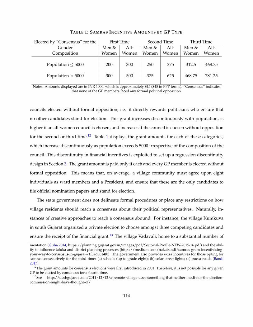
TABLE 1: SAMRAS INCENTIVE AMOUNTS BY GP TYPE

Elected by “Consensus” for the First Time Second Time Third TimeGender Men & All- Men & All- Men & All-

Composition Women Women Women Women Women Women

Population 5000 200 300 250 375 312.5 468.75

Population > 5000 300 500 375 625 468.75 781.25

Notes: Amounts displayed are in INR 1000, which is approximately $15 ($45 in PPP terms). “Consensus” indicatesthat none of the GP members faced any formal political opposition.

councils elected without formal opposition, i.e. it directly rewards politicians who ensure that

no other candidates stand for election. This grant increases discontinuously with population, is

higher if an all-women council is chosen, and increases if the council is chosen without opposition

for the second or third time.12 Table 1 displays the grant amounts for each of these categories,

which increase discontinuously as population exceeds 5000 irrespective of the composition of the

council. This discontinuity in financial incentives is exploited to set up a regression discontinuity

design in Section 3. The grant amount is paid only if each and every GP member is elected without

formal opposition. This means that, on average, a village community must agree upon eight

individuals as ward members and a President, and ensure that these are the only candidates to

file official nomination papers and stand for election.

The state government does not delineate formal procedures or place any restrictions on how

village residents should reach a consensus about their political representatives. Naturally, in-

stances of creative approaches to reach a consensus abound. For instance, the village Kumkuva

in south Gujarat organized a private election to choose amongst three competing candidates and

ensure the receipt of the financial grant.13 The village Vadavali, home to a substantial number of

mentation (Guha 2014, https://planning.gujarat.gov.in/images/pdf/Sectorial-Profile-NEW-2015-16.pdf) and the abil-ity to influence taluka and district planning processes (https://medium.com/nakabandi/samras-gram-incentivising-your-way-to-consensus-in-gujarat-71f32d3514f8). The government also provides extra incentives for those opting forsamras consecutively for the third time: (a) schools (up to grade eight); (b) solar street lights; (c) pucca roads (Bandi2013).

12The grant amounts for consensus elections were first introduced in 2001. Therefore, it is not possible for any givenGP to be elected by consensus for a fourth time.

13See http://deshgujarat.com/2011/12/12/a-remote-village-does-something-that-neither-modi-nor-the-election-commission-might-have-thought-of/

114

Hindu and Muslim families, has decided to divide the President’s five year term equally between

a Hindu and Muslim President (two and a half years each).14 However, survey evidence suggests

that it is usually local elites who nominate candidates and mobilize consensus-based support to

ensure receipt of the monetary benefits (Breman 2011, Bandi 2013, Ganguly 2013, Guha 2014).

The political economy literature has consistently documented the substantial authority that

local elites exert over decision making at the community level (Olken 2007, Alatas et al. 2013,

Acemoglu et al. 2014). It is, therefore, unsurprising that village elders and landowning caste

members are reported to be heavily involved in nominating political candidates and mobilizing

consensus-based support for them. For instance, the dominant15 Rajput residents of Gopalpura

GP nominated women belonging to SC and ST groups for election by consensus in 2011.16 This

anecdote is consistent with Breman (2011), who describes the process of nominating candidates

for consensus based elections in four Gujarati villages Gandevigam, Chikhligam, Bardoligam and

Atulgam:

" The dominant caste-class of landowners state in the village assembly (held twice a year) who are go-

ing to be the next sirpanch (President) and members of the village council. It is possible to turn down the

invitation to be nominated ... but alternative names cannot come up in the hearing."

Breman (2011) further describes an underwhelming approach to governance by councils so-

elected:

"In our observation none of the councils in Gandevigam, Chikhligam, Bardoligam or Atulgam has a

record of activity to show that village democracy is indeed practiced. The members are not involved in the

14This decision was made at a town-hall style meeting (gram sabha) in which leaders of all communities par-ticipated. See http://www.ndtv.com/india-news/day-before-riot-gujarat-village-split-sarpanchs-term-for-muslim-hindu-1674486 for more details.

15Dominant in terms of population share and socioeconomic status.16The village has had official elections only thrice after Independence. There are about 290 Rajput families, 125 ST

families and 65 SC families in the village. "During a village meeting, village elders and women suggested that a chanceshould be given to the women of SC and ST families as it would bring a lot of harmony among the villagers. Thesuggestion was readily accepted." For further details, see http://archive.indianexpress.com/news/narmada-s-rajput-village-appoints-tribal-woman-its-sarpanch/889943/

115

handling of local governance, there is no schedule for meetings and business is attended to by the talati, in

charge of administration, and the sirpanch. The latter may be a figurehead only ... where the exercise of

power is firmly in the hands of members (sic) who belong to the dominant caste-class of landowners ... "

These anecdotes do not imply that the rural poor have no space left for assertion, or that po-

litical representatives elected by community consensus cannot increase access to development

programs and improve public good availability. However, political figureheads may lack the will-

ingness to overcome the drawbacks of political and administrative inexperience, a significant de-

terminant of implementation inefficiencies in the Indian village setting (Afridi et al. 2013). Breman

(2011) also describes lack of experience and socioeconomic standing as hindrances in the effective

functioning of political leaders:

"Their problems are manifold: to start with a total ignorance of government programmes and schemes

in stock, when and where to circumvent or manipulate rules and regulations, lack of familiarity how to

wheel and deal with officials, inability to back up action taken with speed money, i.e. a cash flow ’to get their

work done’ and last but not least, missing the poise to walk around with confidence in the corridors of the

bureaucracy."

In sum, the policy of incentivizing consensus-based elections is controversial, because of its

potential to increase the influence of an elite caucus over their community’s choice of political

representation. As discussed above, it can lead to the appointment of political leaders that merely

serve as figureheads. It has also faced criticism from local politicians, who find themselves de-

prived of financial grants simply because the village chose to have an official election. It is exactly

this deprivation that allows the local elite to quash any opposition in the name of obstructing

village development, inhibiting the development of leadership in backward areas (Institute of So-

cial Sciences 2012). However, the impact of these financial incentives on electoral competition,

politician identity and governance is an open empirical question. To date, there do not exist any

studies that quantify the causal impact of these financial grants, a gap that this paper seeks to fill.

116

Data

Multiple datasets were combined before conducting the empirical analysis. The 2001 and 2011

Population Censuses provides village-level characteristics, including demographic information

and public good availability. GP jurisdictions may contain more than one village, and are mapped

to villages using the Local Body Mapping data obtained from the Area Profiler website managed

by the Ministry of Panchayati Raj.

Information on the 2011 GP elections was obtained from the Gujarat State Election Commis-

sion. This includes detailed information on each political candidate for over 75% of GPs, including

reservation category, gender, education and occupation. Since these datasets are available only in

Gujarati, they were manually merged with the Local Body Mapping dataset described above.

Village level income and expenditure receipts were obtained from the office of the Panchayat,

Rural Housing and Rural Development Department. This department manages the Rural Ac-

counts Management System, which keeps track of various categories of expenditure (education,

nutrition, villlage development, etc) and income (grants, taxes, fees, etc) at the village budget on

an annual basis. This study utilizes village level data for the three fiscal years 2013-16.

Information on the generation of workfare employment under NREGA for 2011-16 was ob-

tained from the NREGA Public Data Portal. Gupta & Mukhopadhyay (2014) show that NREGA’s

primary implementation constraint is the supply of work generated by GPs, not demand. There-

fore, I use information on the amount of employment actually generated as the outcome of inter-

est. This includes measures of the number of households who were provided work, as well as the

number of person-days of employment generated each month. To understand whether NREGA

targeting changed as a result of the consensus-based elections, I use information on the amount of

employment provided to women, Scheduled Castes, Scheduled Tribes and Indira Awaas Yojana

(IAY) households.17

17Indira Awaas Yojana (IAY) is a program targeted at reducing homelessness. IAY households are socioeconomicallydisadvantaged groups (SCs, STs, free bonded laborers, and other rural households below the poverty line) that receivefunding to construct housing units.

117

3 Empirical Strategy

This section sets up a regression discontinuity design based on the discontinuous increase in finan-

cial incentives for “consensus”-based elections at the population threshold 5000. The RD design

quantifies the causal impact of the financial incentives on political competition, political selection

and government performance.

3.1 Central Specification

I follow the suggestions of Hahn, Todd, and Van der Klaauw (2001) and Imbens and Lemieux

(2008), and use local linear regressions after restricting attention to a close bandwidth around the

threshold. Optimal bandwidth choice is based on the procedure outlined in Calonico et al. (2014).

The identifying assumption is that unobservables vary smoothly at the cutoff.

Let popGP denote the population under the GP’s jurisdiction. For ease of notation, I define a

rescaled version of the GP population as p

g

=popGP1000 . Restricting attention to observations within

the optimal bandwidth, the empirical specification takes the following form:

E

ig

= � + ↵

0p

g

1[pg

5] + ↵

1(pg

� 5)1[pg

> 5] + �1[pg

> 5] +X

g

+ ✏

ig

E

ig

denotes an electoral outcome, such as the number of candidates standing for election, for

seat i in GP g. This specification includes a constant �, and fits separate linear regressions before

and after the population threshold - the slope coefficient is ↵

0 before the threshold, and ↵

1 after

the threshold. Xg

represents GP-level controls such as the number of villages under the council’s

jurisdiction as well as demographic controls like the proportion of SC and ST residents. Of primary

interest is the � coefficient, which measures discontinuities in E

ig

as GP population exceeds the

policy threshold 5000 (i.e. as g

p

exceeds 5). The � estimates are interpreted as the causal effects

of financial incentives on electoral competition and political selection. Optimal bandwidths are

chosen separately for each outcome, following the procedure prescribed by Calonico et al. (2014).18

Standard errors are clustered at the level of the discrete running variable, GP population.

18Optimal bandwidths are estimated using data on GPs with population within a bandwidth of 1000 around thethreshold 5000. This avoids the inclusion of other population thresholds at which council composition changes.

118

Some electoral outcomes are measured at the GP level, like the total number of council seats

won without formal opposition. For these outcomes, the central specification uses data at the GP

level instead of the seat level:

E

g

= � + ↵

0p

g

1[pg

5] + ↵

1(pg

� 5)1[pg

> 5] + �1[pg

> 5] +X

g

+ ✏

g

The � coefficient measures the causal effect of the grant increase on electoral outcomes, and stan-

dard errors are clustered at the GP population level.

Governance

Four outcomes at the GP level are used to study governance - council expenditure, council income

with a focus on revenue raised by the local council, and NREGA employment generation and

targeting. Annual data on GP income and expenditure is available for the years 2013-16 and data

on NREGA implementation is available for the years 2011-16. As there are significant outliers

in both sets of data, I trim the top 1% of observations from each of the variables. The empirical

specification takes the following form:

S

gy

= � + ↵

0p

g

1[pg

5] + ↵

1(pg

� 5)1[pg

> 5] + �1[pg

> 5] +X

g

+ �

y

+ ✏

gy

S

gy

denotes a governance outcome in GP g in year y, such as income, expenditure or employment

creation. This specification includes a constant �, separate linear regressions before and after the

population threshold (↵0 and ↵

1 denote the slope coefficients before and after respectively), GP

level controls Xg

and year fixed effects �y

. The � coefficient measures discontinuities in S

gy

as GP

population exceeds the policy threshold 5000 (i.e. as gp

exceeds 5), and is interpreted as the causal

effect of the financial incentives on government functioning. Optimal bandwidths are chosen

separately for each outcome, and standard errors are clustered at the level of the discrete running

variable, GP population.

Alternative Explanations

As noted previously, two features of the elected council increase discontinuously as GP popu-

lation exceeds 5000 - the financial incentive for “consensus” elections increases by 50 per cent,

119

and the number of council members increases by 2. This means that the results on electoral and

governance outcomes may be driven by the addition of two council members, not the increase in

the financial grant. I leverage the existence of alternative population thresholds (i.e. those other

than 5000) at which the number of GP members increases by 2. Discontinuity estimates at these

alternate thresholds isolate the impact of additional council members on electoral and governance

outcomes. These estimates are used to show that it is unlikely that additional council members

are driving the effects documented at the threshold 5000.

Panel A of Figure 1 plots the relationship between the number of GP members and population.

We can see that the number of council members is fixed at 7 for GPs with population up to 3000,

and increases by 2 for every thousand people thereafter. Panel B of Figure 1 plots the relationship

between the number of GP seats reserved for women and population. Since the law mandates the

reservation of at least 33 per cent of seats for women, the number of seats reserved for women

increases by one at every population threshold except 5000 and 8000. Figure A.1 shows that the

number of seats reserved for SCs, STs and OBCs does not increase discontinuously at the thresh-

olds 5000 or 8000. Therefore, I estimate the causal impact of two additional council seats (neither

reserved for women) by testing for discontinuities in electoral and governance outcomes at the

threshold 8000.19

The empirical specifications for electoral and governance outcomes (Eig

and S

gy

respectively)

are analogous to those described above:

E

ig

= �8 + �81[pg

> 8] + ↵

08pg1[p

g

8] + ↵

18(pg � 8)1[p

g

> 8] +X

g

+ ✏

ig

S

gy

= �8 + �81[pg

> 8] + ↵

08pg1[p

g

8] + ↵

18(pg � 8)1[p

g

> 8] +X

g

+ �

y

+ ✏

gy

where �8 is a constant, ↵08 and ↵

18 are distinct population slopes before and after the threshold

8000, and X

g

represents GP-level demographic controls. The �8 coefficient measures the impact

of two additional unreserved seats. Optimal bandwidths are chosen separately for each outcome,

following the procedure prescribed by Calonico et al. (2014).20 Standard errors are clustered at the

19This implicitly assumes that the interaction effects of the higher incentive and additional members are negligible.20Optimal bandwidths are estimated using data on GPs with population within a bandwidth of 1000 around the

threshold 8000. This avoids the inclusion of other population thresholds at which council composition changes.

120

level of the running variable, GP population.

4 Results

This section presents estimates of the effect of increased financial incentives for “consensus”-based

elections. The financial incentive reduces political competition by reducing the number of candi-

dates standing for election for each seat, and increasing the number of seats won without formal

opposition at the GP level. The incentive also crowds in a younger, more educated candidate pool;

politicians who are ultimately elected from this pool are, on average, 4 years younger and have 2

more years of education. Finally, the impact on multiple measures of governance, including local

government expenditure and the targeting of workfare employment, is negative and substantive.

4.1 Baseline Continuity Tests

I first test for evidence of sorting around the population cutoff. This is because GPs may want

to be listed as having more than 5000 residents to receive larger samras grant amounts. This

is unlikely to be the case, however, because the running variable is taken from the Population

Census that was conducted 10 years prior to the introduction of the discontinuous incentives.

Figure A.2 presents the density of population surrounding the two cutoffs used in the analysis.

Population is collapsed into bins of width 20, and no discontinuity in the vicinity of either of the

thresholds is evident. Since the running variable is discrete, I follow Frandsen (2016) to test for the

manipulation of reported population close to the cutoffs.21 The hypothesis of no discontinuity at

the threshold 5000 is not rejected at standard significance levels.22

Next, I show that village demographics and public good availability are balanced at baseline

(in 2011) by testing for discontinuities at the thresholds 5000 and 8000. These balance tests use

information from the 2011 Population Census and are presented in Table A.1. Among the fifty

four tests, six yield statistically significant estimates, which is unsurprising and to be expected

21The McCrary (2008) test, which is commonly used to test for sorting around thresholds, assumes a continuousrunning variable. In the case of a discrete running variable, it may falsely reject the null of no manipulation at too higha rate.

22Figure A.2 displays p-values from the Frandsen (2016) test for discontinuities at the thresholds 5000 and 8000.

121

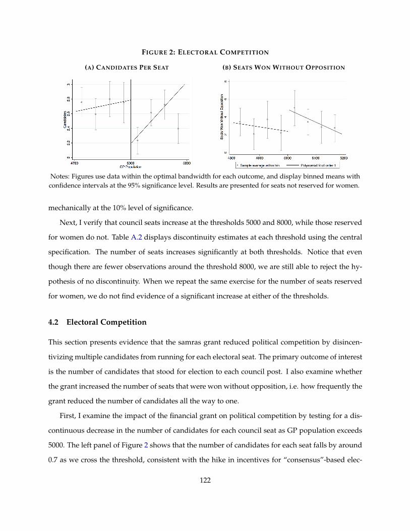
FIGURE 2: ELECTORAL COMPETITION

(A) CANDIDATES PER SEAT (B) SEATS WON WITHOUT OPPOSITION

Notes: Figures use data within the optimal bandwidth for each outcome, and display binned means withconfidence intervals at the 95% significance level. Results are presented for seats not reserved for women.

mechanically at the 10% level of significance.

Next, I verify that council seats increase at the thresholds 5000 and 8000, while those reserved

for women do not. Table A.2 displays discontinuity estimates at each threshold using the central

specification. The number of seats increases significantly at both thresholds. Notice that even

though there are fewer observations around the threshold 8000, we are still able to reject the hy-

pothesis of no discontinuity. When we repeat the same exercise for the number of seats reserved

for women, we do not find evidence of a significant increase at either of the thresholds.

4.2 Electoral Competition

This section presents evidence that the samras grant reduced political competition by disincen-

tivizing multiple candidates from running for each electoral seat. The primary outcome of interest

is the number of candidates that stood for election to each council post. I also examine whether

the grant increased the number of seats that were won without opposition, i.e. how frequently the

grant reduced the number of candidates all the way to one.

First, I examine the impact of the financial grant on political competition by testing for a dis-

continuous decrease in the number of candidates for each council seat as GP population exceeds

5000. The left panel of Figure 2 shows that the number of candidates for each seat falls by around

0.7 as we cross the threshold, consistent with the hike in incentives for “consensus”-based elec-

122

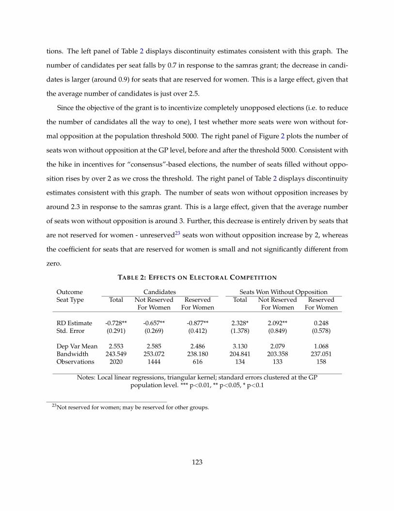
tions. The left panel of Table 2 displays discontinuity estimates consistent with this graph. The

number of candidates per seat falls by 0.7 in response to the samras grant; the decrease in candi-

dates is larger (around 0.9) for seats that are reserved for women. This is a large effect, given that

the average number of candidates is just over 2.5.

Since the objective of the grant is to incentivize completely unopposed elections (i.e. to reduce

the number of candidates all the way to one), I test whether more seats were won without for-

mal opposition at the population threshold 5000. The right panel of Figure 2 plots the number of

seats won without opposition at the GP level, before and after the threshold 5000. Consistent with

the hike in incentives for “consensus”-based elections, the number of seats filled without oppo-

sition rises by over 2 as we cross the threshold. The right panel of Table 2 displays discontinuity

estimates consistent with this graph. The number of seats won without opposition increases by

around 2.3 in response to the samras grant. This is a large effect, given that the average number

of seats won without opposition is around 3. Further, this decrease is entirely driven by seats that

are not reserved for women - unreserved23 seats won without opposition increase by 2, whereas

the coefficient for seats that are reserved for women is small and not significantly different from

zero.

TABLE 2: EFFECTS ON ELECTORAL COMPETITION

Outcome Candidates Seats Won Without OppositionSeat Type Total Not Reserved Reserved Total Not Reserved Reserved

For Women For Women For Women For Women

RD Estimate -0.728** -0.657** -0.877** 2.328* 2.092** 0.248Std. Error (0.291) (0.269) (0.412) (1.378) (0.849) (0.578)

Dep Var Mean 2.553 2.585 2.486 3.130 2.079 1.068Bandwidth 243.549 253.072 238.180 204.841 203.358 237.051Observations 2020 1444 616 134 133 158

Notes: Local linear regressions, triangular kernel; standard errors clustered at the GPpopulation level. *** p<0.01, ** p<0.05, * p<0.1

23Not reserved for women; may be reserved for other groups.

123

4.3 Political Selection

This section examines the impact of lower electoral competition on politician identity, as captured

by the observable characteristics of elected leaders. These characteristics include age, years of edu-

cation, gender and primary occupation. The reduction in political competition ushers in younger,

more educated representatives, but does not significantly increase the proportion of female politi-

cians. I also test for effects on occupation, and find that the grant does not increase the proportion

of candidates from farming and business, which are indicative of elite status within Indian vil-

lages (Bhattacharya et al. 2016). Therefore, even though qualitative evidence suggests that the

local elite have a greater say in “consensus”-based elections, I find suggestive evidence that they

do not crowd themselves into political office.

The first set of results shows the impact of the samras grant on age, education, gender and

occupational status of candidates for council seats. Table 3 displays discontinuity estimates at

the threshold 5000 for all council seats, council seats not reserved for women and council seats re-

served for women. The grant crowds in younger, more educated candidates, but does not increase

the proportion of female candidates. The proportion of candidates that report either farming or

business as their primary occupation (indicative of elite status) does not increase - in fact the esti-

mate is negative, but not significantly different from zero.

All of the above effects are driven by seats that are not reserved for women. This is consis-

tent with the finding that the number of female-reserved seats won without opposition does not

increase in response to the grant. Among seats that are not reserved for women, candidate age

decreases by 3 years and years of education increases by 1.9. Despite the additional incentives

for female candidates, I do not find any evidence that the samras grant crowded female repre-

sentatives into seats not reserved specifically for them. The top panel of Figure 3 displays the

discontinuous change in candidate age and educational achievement for unreserved seats graph-

ically.

Next, I examine whether changes in the candidate pool translated into a change in politician

identity. Table 4 repeats the above analysis, but for politician (i.e. eventual winner) characteristics

instead of candidate characteristics. Politicians are significantly younger, by an average of over 4

124

FIGURE 3: CANDIDATE & POLITICIAN SELECTION EFFECTS

(A) CANDIDATE EDUCATION (B) CANDIDATE AGE

(C) WINNER EDUCATION (D) WINNER AGE

Notes: Figures use data within the optimal bandwidth for each outcome, and display binned means withconfidence intervals at the 95% significance level. Results are presented for seats not reserved for women.

125

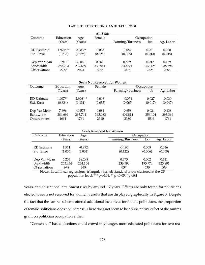
TABLE 3: EFFECTS ON CANDIDATE POOL

All SeatsOutcome Education Age Female Occupation

(Years) (Years) Farming/Business Job Ag. Labor

RD Estimate 1.924*** -2.383** -0.033 -0.089 0.021 0.020Std. Error (0.738) (1.198) (0.025) (0.065) (0.013) (0.045)

Dep Var Mean 6.917 39.862 0.361 0.569 0.017 0.129Bandwidth 258.203 239.669 333.544 340.671 267.425 238.796Observations 2257 2093 2768 2818 2326 2086

Seats Not Reserved for WomenOutcome Education Age Female Occupation

(Years) (Years) Farming/Business Job Ag. Labor

RD Estimate 1.907*** -2.996*** 0.006 -0.074 0.027 0.030Std. Error (0.634) (1.131) (0.035) (0.065) (0.017) (0.047)

Dep Var Mean 7.696 40.573 0.084 0.658 0.024 0.138Bandwidth 284.694 295.744 395.083 404.814 256.101 295.369Observations 1691 1761 2310 2380 1549 1761

Seats Reserved for WomenOutcome Education Age Occupation

(Years) (Years) Farming/Business Job Ag. Labor

RD Estimate 1.511 -0.992 -0.160 0.008 0.016Std. Error (1.055) (2.002) (0.122) (0.006) (0.059)

Dep Var Mean 5.203 38.298 0.373 0.002 0.111Bandwidth 253.434 234.164 236.590 195.774 225.881Observations 678 629 637 530 608

Notes: Local linear regressions, triangular kernel; standard errors clustered at the GPpopulation level. *** p<0.01, ** p<0.05, * p<0.1

years, and educational attainment rises by around 1.7 years. Effects are only found for politicians

elected to seats not reserved for women, results that are displayed graphically in Figure 3. Despite

the fact that the samras scheme offered additional incentives for female politicians, the proportion

of female politicians does not increase. There does not seem to be a substantive effect of the samras

grant on politician occupation either.

“Consensus”-based elections could crowd in younger, more educated politicians for two rea-

126

sons. First, the majority of rural residents may consider these characteristics to be desirable for an

effective political leader, and public deliberation helps shift candidates with these characteristics

into political office. Under this hypothesis, we would expect to see GPs that face higher samras

grants enjoying better governance than GPs that face lower grants. Second, local elites may nom-

inate younger, inexperienced candidates that serve as political figureheads. This explanation is

consistent with survey evidence that the grant amount is only used to justify nominations by the

local elite, who threaten detractors in the name of village development. Under this scenario, we

would not expect to see governance improve. In order to separate between the two hypotheses

and determine whether “consensus”-based elections have had a beneficial impact on governance,

I turn to four measures of the performance of the elected council.

4.4 Governance

This section shows that GPs that faced higher samras grants differ systematically in terms of gov-

ernance. Total expenditure in the GP is significantly lower, and this decrease is driven by ex-

penditure categories that are directly controlled by the elected council. The targeting of workfare

employment, a direct responsibility of the elected council, also worsens.

4.4.1 GP Income and Expenditure

I first examine effects of the samras grant on GP expenditure and its components. The first two

columns of Table 5 display estimates of discontinuities in total and "own fund" expenditure as GP

population exceeds 5000. Own fund expenditure refers to all expense categories that are decided

upon by the elected council such as program expenses of the agriculture, education and health

departments, as well as salaries and other administrative expenses. The elected council has limited

influence over the remaining expense categories, since these are chosen by and tied to grants

received from the state and central government. The first column shows that total expenditure

decreases significantly and substantively - by over half of the mean. The second column shows

that this decrease is driven by a significant drop in own fund expenses. That is, spending on local

administration and development of the village falls as well. The upper panel of Figure 4 displays

127

FIGURE 4: GP EXPENDITURE & INCOME

(A) TOTAL EXPENDITURE (B) OWN FUND EXPENDITURE

(C) TOTAL INCOME (D) OWN FUND INCOME

128

TABLE 4: EFFECTS ON POLITICIAN IDENTITY

All SeatsOutcome Education Age Female Occupation

(Years) (Years) Farming/Business Job Ag. Labor

RD Estimate 1.653** -4.299** -0.024 -0.066 0.007 -0.016Std. Error (0.699) (1.720) (0.031) (0.066) (0.016) (0.055)

Dep Var Mean 7.014 39.767 0.357 0.579 0.016 0.124Bandwidth 354.939 195.636 240.019 358.748 284.026 234.337Observations 2773 1644 2006 2847 2316 1946

Seats Not Reserved for WomenOutcome Education Age Female Occupation

(Years) (Years) Farming/Business Job Ag. Labor

RD Estimate 2.122*** -5.660*** 0.042 -0.106 0.008 0.002Std. Error (0.721) (1.520) (0.038) (0.081) (0.023) (0.050)

Dep Var Mean 7.828 40.502 0.066 0.674 0.023 0.134Bandwidth 314.098 224.284 218.639 307.208 281.295 273.452Observations 1723 1293 1248 1697 1571 1536

Seats Reserved for WomenOutcome Education Age Occupation

(Years) (Years) Farming/Business Job Ag. Labor

RD Estimate 0.829 -1.881 -0.147 0.000 -0.029Std. Error (1.079) (2.799) (0.134) (0.000) (0.085)

Dep Var Mean 5.283 38.203 0.377 0.001 0.101Bandwidth 319.066 224.893 227.502 215.847 227.946Observations 808 587 587 561 587

Notes: Local linear regressions, triangular kernel; standard errors clustered at the GPpopulation level. *** p<0.01, ** p<0.05, * p<0.1

these discontinuity estimates graphically.

Is a decrease in council income driving the negative coefficients on expenditure? The third

column of Table 5 shows that total income does not decrease significantly as population exceeds

the threshold 5000. This estimate is negative, but not significantly different from zero and much

smaller in magnitude than the fall in expenditure. As discussed previously, councils receive grants

from state and national governments, but also collect taxes within their jurisdiction. Since political

129

experience and socioeconomic standing may aid in the generation of government revenue, I exam-

ine whether "own fund" revenue changes discontinuously as population exceeds 5000. Own fund

revenue includes revenue generated through the collection of taxes, fees and other charges. The

last column of Table 5 shows that the effect on own fund revenue is negative and sizable (around

45 per cent of the mean), but not statistically significant. The lower panel of Figure 4 displays

these discontinuity estimates graphically.

TABLE 5: EFFECTS ON INCOME AND EXPENDITURE

Outcome Expenditure IncomeTotal Own Fund Grant Total Own Fund Grant

RD Estimate -12.13* -4.222* 1.000 -3.621 -6.474 -1.511Std. Error (7.006) (2.424) (2.333) (4.763) (5.653) (2.274)

Dep Var Mean 21.522 6.858 11.826 20.903 14.110 5.769Bandwidth 219.733 213.769 314.766 254.541 236.877 268.096Observations 395 384 540 455 421 475

Notes: Local linear regressions, triangular kernel; standard errors clustered at the GPpopulation level. *** p<0.01, ** p<0.05, * p<0.1

4.4.2 Employment Creation Under NREGA

The National Rural Employment Guarantee Act is intended to guarantee one hundred days of em-

ployment to each rural household, in order to complement market demand for labor and provide

income insurance for families close to the poverty line. In practice, the amount and targeting of

work provided is left up to local implementing authorities, and heavily influenced by the elected

GP (Gupta & Mukhopadhyay 2014). Since the Act is entirely funded by the central government,

the GP’s main role is to formulate plans for worksites based on the needs of the village, petition

for funding from higher level authorities and choose program beneficiaries.

I examine four measures of annual employment generation by the council in Table 6 - the

number of households employed, how many of these are SC, ST and IAY households, the number

of person-days of employment generated, and how many of these are allocated towards SCs, STs

and women.24 The effect of the samras grant on overall employment creation is negative but not

24The NREGA implementation data does not contain information on the number of women-only households pro-

130

FIGURE 5: WORKFARE EMPLOYMENT: CREATION AND TARGETING

(A) NON-SC/ST HOUSEHOLDS (B) SC/ST HOUSEHOLDS

(C) NON-SC/ST PERSON-DAYS (D) SC/ST PERSON-DAYS

significantly different from zero. Targeting, however, is clearly negatively affected - the number of

SC and ST households and person-days decrease discontinuously. The estimates are large - over

fifty per cent of the mean in each case - and statistically different from zero. Figure 5 displays

graphical estimates for a subset of these outcomes.

4.5 Ruling Out Alternative Explanations

To ensure that these results are not driven by either the change in council size or council reserva-

tions, I repeat the above exercises for the population threshold 8000. The number of council seats

increases discontinuously at the threshold 8000, while the number of seats reserved for women

vided employment, or person-days allocated towards IAY beneficiaries.

131

TABLE 6: EFFECTS ON EMPLOYMENT CREATION AND TARGETING

Households Employed

Category Total Scheduled Caste Scheduled Tribe Land Reform

RD Estimate -19.82 -4.399** -11.180* -0.228Std. Error (15.206) (2.089) (6.360) (0.152)

Dep Var Mean 55.726 3.042 21.885 0.412Bandwidth 188.963 213.295 278.014 165.483Observations 620 728 943 573

Person-Days of Employment

Category Total Scheduled Caste Scheduled Tribe Women

RD Estimate -7.056 -1.408* -6.414** 1.088Std. Error (6.694) (0.760) (3.149) (2.782)

Dep Var Mean 21.789 1.224 7.818 9.547Bandwidth 189.912 231.675 257.836 372.755Observations 619 779 870 1213

Notes: Local linear regressions, triangular kernel; standard errors clusteredat the GP population level. *** p<0.01, ** p<0.05, * p<0.1

does not. Moreover, the samras grant does not change at this threshold. Therefore, discontinuity

estimates at the threshold 8000 represent the effect of increasing council size alone. I find that the

pattern of results documented at the threshold 5000 are not present at the threshold 8000. That

is, it is likely that the samras grant is driving the reduction in political competition, change in

politician identity and worsening of governance.

Estimates of the effect of council size on electoral competition are presented in Table A.3. None

of the coefficients are statistically significant25 and the coefficient measuring the drop in the num-

ber of candidates per seat is less than 0.1. Tables A.4 and A.5 present estimates of the effect of

council size on candidate and politician characteristics. None of the coefficients are statistically

25Table A.2 shows that this cannot be attributed to the fact that there are fewer observations around the threshold8000. Despite the smaller number of observations, we can strongly reject the hypothesis that the number of councilmembers does not increase at the threshold 8000.

132

significant, and the coefficient on age in particular is much smaller in magnitude than those found

at the threshold 5000.

Turning to measures of government performance, Table A.6 shows that the pattern of results

found at the threshold 5000 is not replicated. The impact of council size on overall and own fund

expenditure is negative but not significantly different from zero. Instead, the coefficient on total

income is negative and statistically significant. The decrease in own fund income remains statis-

tically indistinguishable from zero. Finally, Table A.7 presents estimates of the impact of council

size on employment creation and targeting under NREGA. I find that an increase in council size

alone cannot explain the effects found at the threshold 5000, since none of the coefficients are

statistically significant and many are positive, which is the opposite of the effect documented at

the threshold 5000. Altogether, these results indicate that the reduction in political competition,

crowding in of younger, more educated politicians and worsening of governance is due to the

increase in the “consensus” election grant.

5 Conclusion

This paper quantifies the impact of encouraging the selection of political representatives via com-

munity consensus, as opposed to a secret ballot election, on both the pool of candidates and politi-

cians that are eventually elected. It also examines the effects of encouraging such elections on

multiple measures of governance. The analysis makes use of a novel dataset containing detailed

information on candidates, politicians and government functioning at the village level in the state

of Gujarat in India for the period 2011-15.

To retrieve causal estimates, I exploit the existence of a population threshold at which financial

incentives for “consensus”-based elections sharply increase. The results indicate that financial in-

centives can induce village electorates to choose their political leaders without formal opposition.

I also find that the reduction in competition crowds in younger, more educated candidates and

politicians. Finally, I study four measures of governance over which the elected council exercises

substantial influence, and find a significant reduction in total expenditure as well as an increase

in how regressively workfare employment is targeted. These findings are consistent with the fact

133

that politicians that rely on the support of local elites, who have a greater say in elections based

on community “consensus”, are not incentivized to appease the majority of village residents.

References

ACEMOGLU, DARON, & ROBINSON, JAMES A. 2008. Persistence of Power, Elites, and Institutions. American Economic

Review, 98(1), 267–93.

ACEMOGLU, DARON, REED, TRISTAN, & ROBINSON, JAMES A. 2014. Chiefs: Economic Development and Elite Control

of Civil Society in Sierra Leone. Journal of Political Economy, 122(2), 319–368.

AFRIDI, FARZANA, IVERSEN, VEGARD, & SHARAN, M.R. 2013. Women Political Leaders, Corruption and Learning: Evi-

dence from a Large Public Program in India. IZA Discussion Papers 7212. Institute for the Study of Labor (IZA).

ALATAS, VIVI, BANERJEE, ABHIJIT, HANNA, REMA, OLKEN, BENJAMIN A., PURNAMASARI, RIRIN, & WAI-POI,

MATTHEW. 2013 (February). Does Elite Capture Matter? Local Elites and Targeted Welfare Programs in Indonesia. Working

Paper 18798. National Bureau of Economic Research.

BALAND, JEAN-MARIE, & ROBINSON, JAMES A. 2012. The Political Value of Land: Political Reform and Land Prices

in Chile. American Journal of Political Science, 56(3), 601–619.

BANDI, MADHUSUDAN. 2013. Samras in Gujarat Gram Panchayats: Threat to the Idea of Democracy?

BANERJEE, A., KUMAR, V. S., PANDE, R., & SU, F. 2011. Do Informed Voters Make Better Choices? Experimental

Evidence from Urban India.

BANERJEE, ABHIJIT V, DUFLO, ESTHER, IMBERT, CLEMENT, & PANDE, ROHINI. 2017. Entry, Exit and Candidate Selec-

tion: Evidence from India.

BARDHAN, PRANAB. 2002. Decentralization of Governance and Development. Journal of Economic Perspectives, 16(4),

185–205.

BARDHAN, PRANAB, & MOOKHERJEE, DILIP. 2006. Decentralisation and Accountability in Infrastructure Delivery in

Developing Countries*. The Economic Journal, 116(508), 101–127.

BEATH, ANDREW, CHRISTIA, FOTINI, & ENIKOLOPOV, RUBEN. 2013 (Jan.). Direct Democracy and Resource Allocation:

Experimental Evidence from Afghanistan. Working Papers w0192. Center for Economic and Financial Research (CEFIR).

BESLEY, TIMOTHY, & COATE, STEPHEN. 1997. An Economic Model of Representative Democracy. The Quarterly Journal

of Economics, 112(1), 85–114.

134

BESLEY, TIMOTHY, PANDE, ROHINI, RAHMAN, LUPIN, & RAO, VIJAYENDRA. 2004. The Politics of Public Good Provi-

sion: Evidence from Indian Local Governments. Journal of the European Economic Association, 2(2-3), 416–426.

BESLEY, TIMOTHY, PANDE, ROHINI, & RAO, VIJAYENDRA. 2005. PARTICIPATORY DEMOCRACY IN ACTION: SUR-

VEY EVIDENCE FROM SOUTH INDIA. Journal of the European Economic Association, 3(2-3), 648–657.

BESLEY, TIMOTHY, PERSSON, TORSTEN, & STURM, DANIEL M. 2010. Political Competition, Policy and Growth: Theory

and Evidence from the US. The Review of Economic Studies, 77(4), 1329.

BHATTACHARYA, ANINDYA, KAR, ANIRBAN, & NANDI, ALITA. 2016. Local Institutional Structure and Clientelist

Access to Employment: The Case of MGNREGS in Three States of India. Working Paper No. 269, Centre for Development

Economics, Delhi School of Economics.

BREMAN, JAN. 2011. From Exploitation to Protection? The Impact of the Social Security Bill (2008) for Informal Sector

Workers Report of a Field Study. Amsterdam Institute for Social Science Research (AISSR) Paper.

CAEYERS, BET, & DERCON, STEFAN. 2012. Political Connections and Social Networks in Targeted Transfer Programs:

Evidence from Rural Ethiopia. Economic Development and Cultural Change, 60(4), 639–675.

CALONICO, SEBASTIAN, CATTANEO, MATIAS, & TITIUNIK, ROCIO. 2014. Robust Nonparametric Confidence Intervals

for RegressionâDiscontinuity Designs. Econometrica, 82, 2295–2326.

CASELLI, FRANCESCO, & MORELLI, MASSIMO. 2004. Bad politicians. Journal of Public Economics, 88(3-4), 759–782.

CHATTOPADHYAY, RAGHABENDRA, & DUFLO, ESTHER. 2004. Women as Policy Makers: Evidence from a Randomized

Policy Experiment in India. Econometrica, 72(5), 1409–1443.

DIERMEIER, DANIEL, KEANE, MICHAEL, & MERLO, ANTONIO. 2005. A Political Economy Model of Congressional

Careers. American Economic Review, 95(1), 347–373.

DUNNING, THAD, & NILEKANI, JANHAVI. 2013. Ethnic Quotas and Political Mobilization: Caste, Parties, and Distri-

bution in Indian Village Councils. American Political Science Review, 107(2), 35–56.

FERRAZ, CLAUDIO, & FINAN, FREDERICO. 2009 (April). Motivating Politicians: The Impacts of Monetary Incentives on

Quality and Performance. Working Paper 14906. National Bureau of Economic Research.

FRANDSEN, B. R. 2016. Party Bias in Union Representation Elections: Testing for Ma- nipulation in the Regression

Discontinuity Design When the Running Variable is Discrete. Working Paper.

GANGULY, VARSHA. 2013. State’s Initiatives for Strengthening Local Governance and Impact on Women’s Development

and Empowerment. mimeo, Institute of Rural Research and Development (IRRAD).

135

GUHA, ATULAN. 2014. Undermining Panchayati Raj Institutions in Gujarat. Economic Political Weekly, 49(May).

GUPTA, BHANU, & MUKHOPADHYAY, ABHIROOP. 2014. Local funds and political competition: Evidence from the

National Rural Employment Guarantee Scheme in India. ESID Working Paper 42.

HINNERICH, BJÖRN TYREFORS, & PETTERSSON-LIDBOM, PER. 2014. Democracy, Redistribution, and Political Partici-

pation: Evidence From Sweden 1919–1938. Econometrica, 82(3), 961–993.

IMBERT, CLÉMENT, & PAPP, JOHN. 2015. Labor Market Effects of Social Programs: Evidence from India’s Employment

Guarantee. American Economic Journal: Applied Economics, 7(2), 233–63.

INSTITUTE OF SOCIAL SCIENCES, . 2012. Panchayati Raj Update. XIX(January).

KEANE, MICHAEL P., & MERLO, ANTONIO. 2010. Money, Political Ambition, and the Career Decisions of Politicians.

American Economic Journal: Microeconomics, 2(3), 186–215.

KHWAJA, ASIM IJAZ. 2004. Is Increasing Community Participation Always a Good Thing? Journal of the European

Economic Association, 2(2-3), 427–436.

LEE, DAVID S. 2008. Randomized Experiments from Non-random Selection in U.S. House Elections. Journal of Econo-

metrics, 142(2), 675–697.

LIZZERI, ALESSANDRO, & PERSICO, NICOLA. 2005. A Drawback of Electoral Competition. Journal of the European

Economic Association, 3(6), 1318–1348.

MATTOZZI, ANDREA, & MERLO, ANTONIO. 2008. Political careers or career politicians? Journal of Public Economics,

92(3-4), 597–608.

MCCRARY, JUSTIN. 2008. Manipulation of the running variable in the regression discontinuity design: A density test.

Journal of Econometrics, 142(2), 698 – 714. The regression discontinuity design: Theory and applications.

OLKEN, BENJAMIN A. 2007. Monitoring Corruption: Evidence from a Field Experiment in Indonesia. Journal of Political

Economy, 115(2), 200–249.

OLKEN, BENJAMIN A. 2008 (June). Direct Democracy and Local Public Goods: Evidence from a Field Experiment in Indonesia.

Working Paper 14123. National Bureau of Economic Research.

OSBORNE, MARTIN, & SLIVINSKI, AL. 1996. A Model of Political Competition with Citizen-Candidates. The Quarterly

Journal of Economics, 111(1), 65–96.

PANDE, ROHINI. 2003. Can Mandated Political Representation Increase Policy Influence for Disadvantaged Minorities?

Theory and Evidence from India. The American Economic Review, 93(4), 1132–1151.

136

PETTERSSON-LIDBOM, PER. 2012. Does the size of the legislature affect the size of government? Evidence from two

natural experiments. Journal of Public Economics, 96(3), 269–278.

POWLEY, E. 2007. Rwanda: The Impact of Women Legislators on Policy Outcomes Affecting Children and Families. In:

Background Paper. State of the World’s Children.

RAJARAMAN, I., & GUPTA, M. 2012. Public expenditure choices and gender quotas. Indian Growth and Development

Review, 5(2): 108-130.

RAO, VIJAYENDRA, & IBÁÑEZ, ANA MARÍA. 2005. The Social Impact of Social Funds in Jamaica: A ‘Participatory

Econometric’ Analysis of Targeting, Collective Action, and Participation in Community-Driven Development. The

Journal of Development Studies, 41(5), 788–838.

WASHINGTON, EBONYA L. 2008. Female Socialization: How Daughters Affect Their Legislator Fathers’ Voting on

Women’s Issues. The American Economic Review, 98(1), 311–332.

137

Appendix

138

FIGURE A.1: COUNCIL MEMBER RESERVATIONS & GP POPULATION

Notes: GP Seats reserved for Scheduled Castes, Scheduled Tribes and Other Backward Castes do not increase discontinuously at the population thresholds5000 and 8000.

139

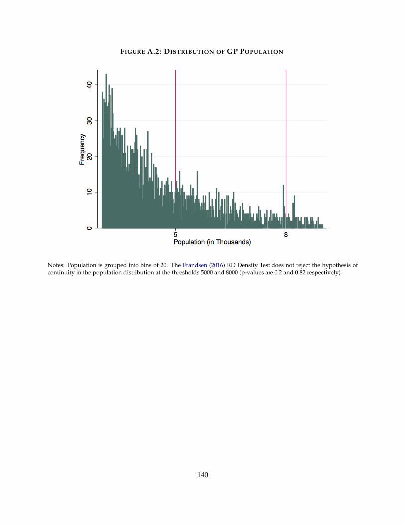
FIGURE A.2: DISTRIBUTION OF GP POPULATION

Notes: Population is grouped into bins of 20. The Frandsen (2016) RD Density Test does not reject the hypothesis ofcontinuity in the population distribution at the thresholds 5000 and 8000 (p-values are 0.2 and 0.82 respectively).

140

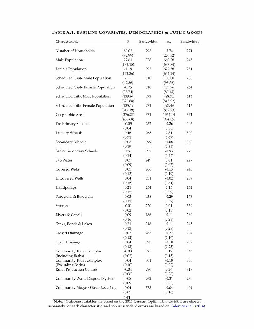
TABLE A.1: BASELINE COVARIATES: DEMOGRAPHICS & PUBLIC GOODS

Characteristic � Bandwidth �8 Bandwidth

Number of Households 80.02 293 -5.74 271(82.99) (220.32)

Male Population 27.61 378 660.28 245(183.15) (637.84)

Female Population -1.18 393 622.58 251(172.36) (654.24)

Scheduled Caste Male Population -1.1 310 100.00 268(42.36) (93.59)

Scheduled Caste Female Population -0.75 310 109.76 264(38.74) (87.45)

Scheduled Tribe Male Population -133.67 273 -88.74 414(320.88) (845.92)

Scheduled Tribe Female Population -135.19 271 -97.49 416(319.19) (857.73)

Geographic Area -276.27 371 1554.14 371(438.68) (994.85)

Pre-Primary Schools -0.05 252 -0.26 405(0.04) (0.35)

Primary Schools 0.46 263 2.51 300(0.71) (1.67)

Secondary Schools 0.03 399 -0.08 348(0.19) (0.35)

Senior Secondary Schools 0.26 397 -0.93 273(0.14) (0.42)

Tap Water 0.05 249 0.01 227(0.09) (0.07)

Covered Wells 0.05 266 -0.13 246(0.13) (0.19)

Uncovered Wells 0.04 331 -0.02 239(0.15) (0.31)

Handpumps 0.21 254 0.13 262(0.12) (0.29)

Tubewells & Borewells 0.03 438 -0.29 176(0.12) (0.32)

Springs -0.01 220 0.01 339(0.02) (0.18)

Rivers & Canals 0.09 186 -0.11 269(0.16) (0.28)

Tanks, Ponds & Lakes 0.21 318 -0.11 245(0.13) (0.28)

Closed Drainage 0.07 283 -0.22 204(0.12) (0.16)

Open Drainage 0.04 393 -0.10 292(0.13) (0.25)

Community Toilet Complex -0.03 325 0.19 346(Including Baths) (0.02) (0.15)Community Toilet Complex 0.04 301 -0.10 300(Excluding Baths) (0.10) (0.22)Rural Production Centres -0.04 290 0.26 318

(0.06) (0.28)Community Waste Disposal System 0.08 262 -0.31 230

(0.09) (0.33)Community Biogas/Waste Recycling 0.04 373 -0.04 409

(0.07) (0.16)

Notes: Outcome variables are based on the 2011 Census. Optimal bandwidths are chosenseparately for each characteristic, and robust standard errors are based on Calonico et al. (2014).

141

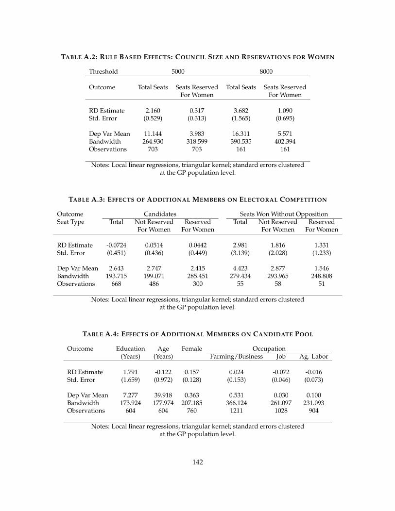
TABLE A.2: RULE BASED EFFECTS: COUNCIL SIZE AND RESERVATIONS FOR WOMEN

Threshold 5000 8000

Outcome Total Seats Seats Reserved Total Seats Seats ReservedFor Women For Women

RD Estimate 2.160 0.317 3.682 1.090Std. Error (0.529) (0.313) (1.565) (0.695)

Dep Var Mean 11.144 3.983 16.311 5.571Bandwidth 264.930 318.599 390.535 402.394Observations 703 703 161 161

Notes: Local linear regressions, triangular kernel; standard errors clusteredat the GP population level.

TABLE A.3: EFFECTS OF ADDITIONAL MEMBERS ON ELECTORAL COMPETITION

Outcome Candidates Seats Won Without OppositionSeat Type Total Not Reserved Reserved Total Not Reserved Reserved

For Women For Women For Women For Women

RD Estimate -0.0724 0.0514 0.0442 2.981 1.816 1.331Std. Error (0.451) (0.436) (0.449) (3.139) (2.028) (1.233)

Dep Var Mean 2.643 2.747 2.415 4.423 2.877 1.546Bandwidth 193.715 199.071 285.451 279.434 293.965 248.808Observations 668 486 300 55 58 51

Notes: Local linear regressions, triangular kernel; standard errors clusteredat the GP population level.

TABLE A.4: EFFECTS OF ADDITIONAL MEMBERS ON CANDIDATE POOL

Outcome Education Age Female Occupation(Years) (Years) Farming/Business Job Ag. Labor

RD Estimate 1.791 -0.122 0.157 0.024 -0.072 -0.016Std. Error (1.659) (0.972) (0.128) (0.153) (0.046) (0.073)

Dep Var Mean 7.277 39.918 0.363 0.531 0.030 0.100Bandwidth 173.924 177.974 207.185 366.124 261.097 231.093Observations 604 604 760 1211 1028 904

Notes: Local linear regressions, triangular kernel; standard errors clusteredat the GP population level.

142

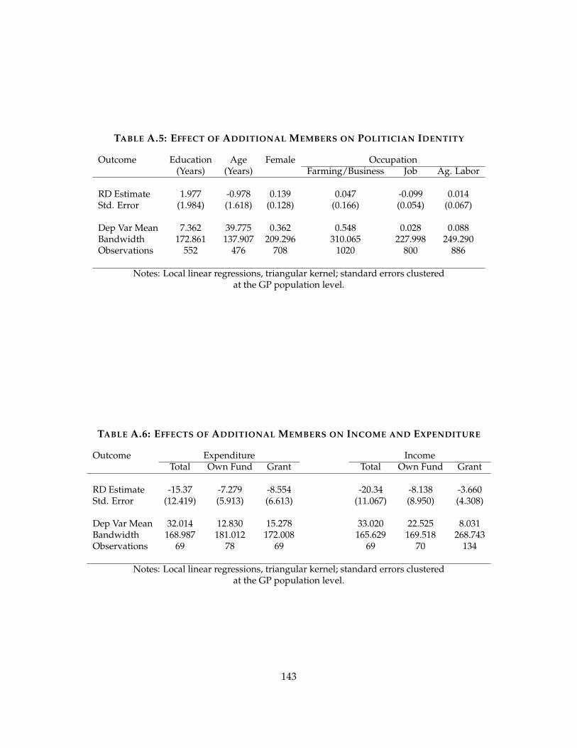
TABLE A.5: EFFECT OF ADDITIONAL MEMBERS ON POLITICIAN IDENTITY

Outcome Education Age Female Occupation(Years) (Years) Farming/Business Job Ag. Labor

RD Estimate 1.977 -0.978 0.139 0.047 -0.099 0.014Std. Error (1.984) (1.618) (0.128) (0.166) (0.054) (0.067)

Dep Var Mean 7.362 39.775 0.362 0.548 0.028 0.088Bandwidth 172.861 137.907 209.296 310.065 227.998 249.290Observations 552 476 708 1020 800 886

Notes: Local linear regressions, triangular kernel; standard errors clusteredat the GP population level.

TABLE A.6: EFFECTS OF ADDITIONAL MEMBERS ON INCOME AND EXPENDITURE

Outcome Expenditure IncomeTotal Own Fund Grant Total Own Fund Grant

RD Estimate -15.37 -7.279 -8.554 -20.34 -8.138 -3.660Std. Error (12.419) (5.913) (6.613) (11.067) (8.950) (4.308)

Dep Var Mean 32.014 12.830 15.278 33.020 22.525 8.031Bandwidth 168.987 181.012 172.008 165.629 169.518 268.743Observations 69 78 69 69 70 134

Notes: Local linear regressions, triangular kernel; standard errors clusteredat the GP population level.

143

TABLE A.7: EFFECTS OF ADDITIONAL MEMBERS ON EMPLOYMENT CREATION

Households Employed

Category Total Scheduled Caste Scheduled Tribe Land Reform

RD Estimate -4.934 0.355 6.146 -0.274Std. Error (30.444) (2.883) (16.785) (0.253)

Dep Var Mean 47.520 2.152 16.222 0.477Bandwidth 328.771 213.385 392.632 231.497Observations 338 220 385 254

Person-Days of Employment

Category Total Scheduled Caste Scheduled Tribe Women

RD Estimate 2.436 0.145 -0.412 -0.474Std. Error (13.005) (0.886) (3.824) (5.820)

Dep Var Mean 18.246 0.733 5.570 8.142Bandwidth 308.807 240.439 305.111 380.111Observations 318 266 318 373

Notes: Local linear regressions, triangular kernel; standard errors clusteredat the GP population level.

144