essays on macro-finance: identification, estimation and ... · instituto nacional de matemática...
TRANSCRIPT

Instituto Nacional de Matemática Pura e Aplicada
Doctoral Thesis
Essays on Macro-Finance: Identification,Estimation and Forecasting of Term StructureModels with Macro Factors and Default Risk
Marco S. Matsumura
Advisor: Aloisio Araujo
September 2008

ii
Thesis committee:
Aloisio Araujo, IMPA & FGV
Caio Ibsen, FGV
Hélio Migon, UFRJ
J. Valentim Vicente, BACEN & IBMEC
Márcio Nakane, USP & BACEN

Dedicado à minha família.
Agradecimentos
Sou especialmente grato a toda comunidade do IMPA, na qualidade de seus pro-fessores, funcionários e colegas, pela oportunidade única na vida de participar deum ambiente tão rico, criativo e estimulante para a pesquisa e muito além, nessesanos cruciais para minha formação, e pelo apoio ágil e ‡exível da instituição nosmomentos importantes. Agradeço ao Professor Aloísio Araújo por sua orientaçãoe grandes ensinamentos, e por toda liberdade de pesquisa que pude, talvez imere-cidamente, desfrutar. Sou grato aos meus Professores de Economia Matemática,Wilfredo Leiva, Paulo Klinger e Humberto Moreira, que me ensinaram os primeirospassos numa área que me era então completamente nova. Agradeço ao ProfessorClaudio Landim, que num curso de verão há tantos foi quem primeiro incentivoua ingressar no IMPA, e que considero o começo de todo o processo que gerou estetrabalho. Agradeço também a todos os Professores e Amigos e Colegas de turma,com os quais sempre procurei aprender o máximo que pude, mas a quem certamentedevo mais do que jamais poderei retribuir. Devo ao IPEA a liberdade com que pudeescolher e manter minha linha de pesquisa desde minha entrada na instituição, e àsótimas condições de trabalho. Agradeço à banca de doutorado, que muito interagiue muito contribuiu nos estágios …nais da preparação deste texto. Fundamentaistambém para a realização deste trabalho foram os apoios das agências de fomentoCNPq e Capes, dos quais fui continuamente bolsista desde meu primeiro ano dagraduação.


Contents
1. General introduction 1
Chapter 1. Assessing Macro In‡uence on Brazilian Yield Curve with A¢neModels 5
1. Introduction 52. A¢ne Model 83. Inference 124. Results 165. Conclusion 27
Chapter 2. The Role of Macroeconomic Variables in Determining SovereignRisk 29
1. Introduction 292. A¢ne Model with Default Risk and Macro Factors 323. Data 354. Estimation 365. Results 416. Conclusion 48
Chapter 3. Identi…cation of Term Structure Models with Observed Factors 531. Introduction 532. Models 533. Identi…cation 544. Conclusion 58
Chapter 4. Forecasting the Yield Curve: Comparing Models 591. Introduction 592. Models 603. Inference 624. Data 655. Estimation 666. Conclusion 71
Chapter 5. Macro-Finance Models Combining Daily and Monthly Data 731. Introduction 732. Term Structure 743. Inference 754. Empirical Analysis 775. Change of regime: Taylor rule switching model and sub-sample 816. Conclusion 82
v

vi C ONTE NT S
Appendix A. Convergence 851. Description of Gelman-Rubin test 852. Simulation exercise 85
Appendix B. References 91

1. GENERAL INTRODUCT ION 1
1. General introduction
This work propose a number of improvements in the area of macro-…nancemodels, which consists of combinations of term structure and macroeconometricmodels.
There are multiple applications of term structure models with di¤erent ends.Some of which are given in the following: 1) …nancial market practitioners needmodels for interest rate and credit risk derivatives; 2) in order for the Central Bankto conduct the monetary policy and monitor the yield curve, it need to know howthe curve is related to macroeconomic indicators; 3) the Treasury continuouslydemands assessments of current and future interest rates to manage the emissionand maintenance of the stock of public debt.
We assess the impact of macro factors on the yield curve of emerging countries,where data is relatively scarce and volatile as compared to developed countries’.Also, frequent changes of regime, crisis episodes and defaults limit the extent of theexisting historical series.
In those markets, the Monetary Authorities may respond to other factors be-sides the expected in‡ation and the output gap. The exchange rate, for instance,is an important variable.
Moreover, the relevance of explicitly including macro factors into the termstructure models may di¤er when dealing with developed or with emerging markets.The …xed income markets are huge and very sophisticated markets in which assetsare traded in almost continuous-time. Do bond investors already process all themarkets information e¢ciently?
In contrast, macroeconomic indicators have a low frequency nature as they mustbe collected and processed by institutions; they are not real-time information. Forthis reason, traditionally the macro-…nance models are discrete-time, and estimatedwith monthly or quarterly data. Ang and Piazzesi (2003) estimated their modelwith a quarterly series containing roughly 50 years of data.
On the other hand, the limitations of emerging market samples may require theuse of daily data. In this case, continuous-time models constitute a natural choice.
In our …rst article, we analyze the relation between the Brazilian domestic termstructure and macroeconomic variables.
We construct a novel dataset consisting of daily samples of 1) DI x Pre interestrate swaps, traded on the BM&F, proxy for zero-coupon constant maturity termstructure, 2) INPC x DI swaps (available since 2002), which provide a measure ofdaily in‡ation, and 3) the US Dollar/ Brazilian Real exchange rate.
We show that the inclusion of macro factors signi…cantly improves the goodness-of-…t of the term structure models by comparing yields alone and macro-augmenteda¢ne models.
Continuous and discrete-time Gaussian a¢ne models are considered. The mea-surement errors are treated with either Kalman …lter or Chen-Scott inversion.Three di¤erent Taylor rules and two di¤erent lag sizes are considered, and theparameters are inferred through maximum likelihood or Monte Carlo Markov chain(MCMC).
Among our empirical …ndings, we remark that macro factors explain about40% of the movements of the yield curve, and that imposing restrictions on thespeci…cation of the model - such as macro-to-yield dynamics or standard Taylor

2 C ONTE NT S
rule - signi…cantly modi…es the response of the yield curve, and should thus becarefully considered.
In chapter two, we extend the models by adding default risk and address theproblem of …nding the factors behind the movements of emerging market sovereigninterest rates. The models are estimated again with daily data, allowing for theinteraction between macro variables and credit spreads.
The emerging markets’ Central Banks do not have direct in‡uence on sovereigninterest rates, which are traded on international markets. Thus, contrary to thedomestic case, there are no obvious candidates as the most important macro factorsin‡uencing the external rates.
We calculate default probabilities implied from the estimated model and theimpact of macro shocks on those probabilities.
Our empirical results show that, given our tested variables and horizon, the VIX(a volatility index calculated using S&P 500 option prices) is the most importantmacro factor a¤ecting short term bonds and default probabilities, while the FedFund is the most important factor behind long term default probabilities. Regardingtested domestic factors, only the slope of the domestic yield curve showed relevante¤ect.
Before estimating the models, they must …rst be identi…ed. In fact, we showthat the likelihood function of the Gaussian a¢ne models with macro factors anddefault using Chen-Scott inversion are invariant to certain operators.
The question of identi…cation is not completely discussed by the literature. Ourcontributions to this topic are the subject of our third article, where we extend themethod of Dai and Singleton (2002) to term structure models with macro factors.
There many possible identi…cations, but we prove that the choice of identi…ca-tion does not a¤ect the response of the yield curve or of the macro factors to statevariable shocks. However, it does a¤ect the latent factor response.
Next, in article four, we focus our attention on the out-of-sample predictivecapacity of a number of term structure models. The models are estimated withBrazilian and U.S. daily samples, so that we obtain results that contrast speci…ccharacteristics of emerging and developed markets data.
In particular, we compare the a¢ne and the Nelson-Siegel models, includingthe Diebold-Li 2-step model, which list among the most popular in the …nancialand econometric literature.
We test whether macro-…nance models outperforms yields alone models. ForBrazil, we consider a version with the IBovespa (Sao Paulo Stock Exchange Index)besides versions with expected in‡ation and output gap.
We show that for U.S. yields-only models already present good performance,and that the addition of macro factors does not improve the predictions.
For Brazilian data, both the yields only or macro-…nance models present lowperformance. However, the IBovespa signi…cantly contributes to the forecastingperformance of the models.
On overall, the best model was the unrestricted dynamic Nelson-Siegel model.In our …nal article, chapter 5, we further examine the properties of the macro-
…nance models proposed in article 4. However, instead of forecasting, our focusturn to calculate impulse response functions and variance decompositions so as toanalyze the nature of the impact of the di¤erent indicators on the yield curves ofboth markets.

1. GENERAL INTRODUCT ION 3
We discuss a novel model combining monthly macro data and daily term struc-ture data (a “pooled” model), which provides more accurate results than purelymonthly models, specially for the case of Brazil.
We also propose a simple extension that incorporates change of regime. Itspeci…cally tries to capture possible changes of monetary policy. It is estimatedwith Greenspan and Bernanke periods, and presidents Lula and Cardoso’s periods.
All models in chapter 4 and 5 are estimated via MCMC. In the appendix weperform a series of simulation exercises were we show that our MCMC algorithmcorrectly recovers the true parameters, and that the chains generated by the Gibbssampling and Metropolis-Hastings converge under the Gelman-Rubin diagnostics.

CHAPTER 1
Assessing Macro In‡uence on Brazilian YieldCurve with A¢ne Models
1. Introduction
The term structure of interest rates synthesizes agents’ perceptions about thefuture state of the economy. The interaction between that perception and macroe-conomic variables is an important element for consideration by the monetary au-thorities (MA) for policy decisions and by market participants for forecasting. Angand Piazzesi (2003), A&P, discuss that interaction proposing a model that combinesideas from the …nancial and the macroeconometric literature.
In the …nancial literature, the a¢ne term structure models (Du¢e and Kan,1996), constitute a popular class of models, in which the yield and the risk premiumsare modeled in continuous time as a¢ne functions of unobserved state variables.However, since standard a¢ne models do not contain macroeconomic variables,they cannot be directly related to the yield curve or latent factors.
Macroeconometric models usually analyze the e¤ect of observed variables onthe yield curve, and model the dynamics of the rates and of the e¤ects of …nancialand macro shocks. But they do not take into account the no-arbitrage restrictionsamong the rates of the diverse maturities, which can potentially lead to an over-parameterization of the model and a reduction of its forecasting capacity.
A&P’s model incorporates observed macro variables - the output gap and in-‡ation - into a discrete-time a¢ne model and a MA reaction function to nominalshocks - the Taylor rule - to study the relation between the economic cycle andthe yield curve. This is an extension of small-scale macro models such as that ofSvensson (1997). In this way, some of the exogenous shocks on the state factorsand their e¤ects on the yield curve become identi…able in a model with no arbitragerestrictions among the yield maturities.
By including macro variables, the task of the inference of the parameters be-comes more di¢cult, due to the nonlinear character of the model. This fact mo-tivated us and Ang et al. (2005) to use the Monte Carlo Markov chain (MCMC)algorithm, a Bayesian approach, which is less vulnerable to dimensional issues thanmaximum likelihood.
Our work addresses the Brazilian market, which requires di¤erent choices offrequency and macro factors. In A&P, the unity of time is the quarter, the frequencywith which the output gap is measured. This is not possible for analyzing theBrazilian economy.
The behavior of emerging countries’ …nancial markets can be distinguished fromthat of developed countries’ markets by the lower liquidity, shorter term structure(less than 3 years until recently), more interventions that result in changes of regime
5

61 . ASSESSING M AC RO INFLUENC E ON B RAZ IL IAN YIELD C URVE WIT H AFFINE M ODELS
and of rules of operation, existence of credit risk in public debt, greater vulnerabilityassociated with volatile exchange rates, and limited data availability.
Also, up to 1994 the Brazilian economy experienced a long period of highin‡ation. In‡ation rates as high as 90% a month occurred during this period.
However, even in this environment, the Central Bank was able to preserve thecredibility of the domestic currency as a denomination of public debt and means oflegal payment, thanks to an ample indexation system that included the Braziliancurrency and the U.S. dollar exchange rate as a reference.
The Real Plan (including introduction of the present currency, the Real) wasimplemented in 1994 as a regime that pegged the domestic currency to the U.S. dol-lar until 1998, drastically reducing the in‡ation rates that prevailed at the time. InJanuary 1999, this …xed exchange rate regime collapsed after a series of speculativeattacks.
After that, the monetary authorities decided to adopt a free exchange ratecombined with in‡ation targeting. The Central Bank issued local currency bondslinked to the dollar exchange rate index. A substantial fraction of the public debtwas indexed to the dollar in this way. Together, these facts attest the importanceof the exchange rate for the Brazilian economy.
One of the tools for monitoring the in‡ation targeting regime was developedby Bogdanski et al (2000). It consists of a macro model similar to that of Svens-son (1997), extended with the e¤ect of currency devaluations on the equation thatdetermines the in‡ation rate. This modi…cation was inspired by an extensive litera-ture on emerging countries (see Fraga et al., 2003). Other articles produced by theBrazilian Central Bank (Almeida et al., 2003, Fachada, 2001, Freitas and Muinhos,2001, Goldfajn and Werlang, 2000, Minella et al., 2003, Muinhos and Alves, 2003,Rodrigues et al., 2000) emphasize the importance of the exchange rate in priceformation.
Backed by that evidence, we choose the in‡ation and exchange rate as ourmacro factors. And since our sample starts only after the alteration of the monetaryregime in 1999, with the adoption of the in‡ation targeting, we use daily data. Theunit of time used in A&P, the quarter (the frequency with which the output gap ismeasured), is not feasible for us.
Also, the sample size does not allow analysis of the iteration between realvariables and the yield curve, in‡ation and exchange rate. Instead, we ignore thereal variables and consider a reduced-form macro model with daily data.
A source of zero-coupon constant maturity rates of Brazilian domestic bondsis the BM&F Bovespa, the São Paulo Stock Exchange, which trades various typesof interest rate swaps. Two of them are used here, the DIxPre and the INPCxDI.The …rst swap trades ‡oating for …xed interest rates, and the second swap yieldsthe ‡oating rate on one side, and the expected consumer price index rates (INPC)on the other. The …rst swap permits the construction of the yield curve, and bothtogether can be used to extract the expected in‡ation for certain horizons. Thetrading volumes of these two swaps are on average about U.S.$30 million each.
By using daily data, we focus on the …nancial, high frequency, aspects of therelation among interest rates, the exchange rate and expected in‡ation, as opposedto macroeconomic, low frequency aspects and larger horizons.
Due to the chosen unit of time, our model omits the output gap, which indicatesthe state of the economic cycle. However, the e¤ect of the output gap is not absent:
1. INT RO DUC T IO N 7
since the yield curve summarizes the state of the economy, the latent factors containinformation from omitted variables, and thus can capture economic cycle e¤ects.
One version of our model, (C), follows the tradition of a large body of …nancialliterature that uses daily samples, speci…es the model in continuous-time and es-timates it via maximum likelihood. Another version, (D), follows the econometrictradition, specifying a discrete-time model, and is estimated through MCMC.
It is not immediately evident how to choose the most adequate speci…cationand method of inference. Other technical questions, such as the forecasting horizonand the de…nition of the latent variable (discussed later), have to be decided byempirical testing. Thus, di¤erent speci…cations are estimated. We discuss thegoodness-of-…t and impulse response functions in such a way that the two versionscan be compared.
Many authors emphasize the importance of incorporating macro variables to…nancial models. For example, Diebold et al. (2005) remarks that pure a¢ne mod-els add little insight into the nature of the underlying economic forces driving theyield curve movements. Adding macro factors would shed light to the fundamentaldeterminants of the interest rates. They point out the importance of the short rateas a fundamental building block to price all the bonds and as a policy instrumentunder direct control of the central bank to achieve its economic stabilization goals.
A&P estimate via maximum likelihood a macro-to-yield model, in the sensethat macro factors a¤ect, but are not a¤ected by, monetary factors. Ang et al.(2005) improve that model by estimating a bidirectional model with one latentfactor and two macro factors using MCMC. They report that the model forecastsbetter than the unrestricted VAR.
Rudebusch and Wu (2003) develop a no arbitrage macro-structural model withmacro variables and latent monetary factors that jointly drive yields. They reportthat output shocks have a signi…cant impact on intermediate yields and curvatureand that in‡ation surprises have large e¤ects on the level of the yield curve. Theyalso …nd that including macro factors improve the forecasts of the usual latentfactor models. Dai and Philippon (2004) estimate a no arbitrage VAR model withone latent factor and government de…cit, in‡ation and real activity. They arguethat the de…cit is an important factor behind the yield curve. Nelson-Siegel modelsare discussed by Diebold et al. (2006).
Wu (2003) considers the impact of macro shocks on U.S. term structure using astructural VAR model, and concludes that monetary-policy and aggregate-supplyshocks are important determinants of the slope and level of the yield curve, re-spectively. Hejazi (2000), on the other hand, examines whether information in theU.S. yield curve can be useful for predicting monthly industrial output. Using aGARCH-M model, he shows that while T-bill spreads contain little or no predictivecontent, increases in term premiums, which are linear functions of the conditionalvariance of excess returns, have predictive content.
Kalev and Inder (2006) and Chen (2001) test the rational expectations theoryusing U.S. term structure data. The former authors investigate how much informa-tion about the future yields is contained in the current spot rates, and their resultssuggest that a signi…cant amount of freely available information is not incorporatedin forming agents’ expectations. The latter author incorporates in‡ation in a modelthat allows for changes in regime, and concludes that the regime-switching modeldoes not reconcile the data with the expectations hypothesis.

81 . ASSESSING M AC RO INFLUENC E ON B RAZ IL IAN YIELD C URVE WIT H AFFINE M ODELS
All these papers use discrete-time model and monthly or quarterly data.To summarize, our objectives include: i) assessing the importance of macro
variables in an a¢ne term structure model for a Brazilian sample; ii) given the highnumber of parameters, evaluating the imposition of restrictions; iii) estimating thee¤ect of the identi…ed shocks, such as the exchange rate and in‡ation, on the yieldcurve, and vice-versa.
We …nd that macro factors improve the performance of the models. Also,variance decompositions show that the macro variables are important factors foryield curve movements in the Brazilian local market, a result that is similar to thatof Diebold et al. (2006) for the U.S. bond market.
Finally, we remark that identi…cation has two meanings here. First, it is usedas in the …nancial context as the elimination of free parameters that cannot beestimated, as in Dai and Singleton (2000). Second, it is used as in the VAR literatureas the exogeneity ordering of the state variables.
2. A¢ne Model
2.1. Continuous-Time. A probability space (, F, P) is …xed and no arbi-trage is assumed. The price at time t of a zero-coupon bond paying $1 at maturitydate t + τ is P (t, τ ) = EQ
hexp
³¡
R t+τt rtdt
´j Ft
i. The conditional expectation
is taken under the equivalent martingale measure Q, and rt is the stochastic in-stantaneous discount rate. Below, we discuss the pricing equations (see also Du¢e,2001).
The vector Xt 2 Rp represents the state of the economy, and the short rateand risk premium process are given by time-varying processes rt = δ0 + δ1 ¢ Xt andλt = λ0 + λ1 ¢ Xt. It is assumed that Xt follows a Gaussian process with meanreversion. Under the objective P-measure,
(2.1) dXt = K(ξ ¡ Xt)dt + §dwt .
The p£p and p£1 parameters K and ξ represent the mean reversion coe¢cient andthe long-term mean short rate, and §§T is the instantaneous variance-covariancematrix of the p-dimensional standard Brownian shocks wt .
By Girsanov, under the martingale measure Q, dXt = K?(ξ? ¡ Xt)dt + §dw?t ,
where dw?t = dwt + λtdt is a standard Q-Brownian motion, and K ? = K + §λ1,
ξ? = K?¡1(Kξ ¡ §λ0).Multifactor Feynman-Kac formula states that, given technical conditions, if
EQhexp
³¡
R t+τt r(Xu)du
´j Ft
i= v(Xt, t, τ), then v(x, t,τ ) must satisfy Dv(x, t, τ )¡
r(x)v(x, t,τ ) = 0, v(x, t,0) = 1, where the operator D is given by
Dv(x, t, τ ) := vt(x, t, τ) + vx(x, t, τ) ¢ K?(ξ? ¡ x) +12tr[§§| vxx(x,t, v)].
Applying Feynman-Kac to our pricing equation, it turns out that P (t, τ , Xt) =eα(τ )+β(τ )¢Xt, where
(2.2) β0(τ) = ¡δ1 ¡ K?|β (τ),
(2.3) α0(τ) = ¡δ0 + ξ?|K ?| β(τ) +12
β(τ)|§§| β(τ ).

2 . AFFINE M ODEL 9
are Riccati di¤erential equations whose explicit solutions exist only in some specialcases, such as when K is diagonal, but Runge-Kutta numerical integration e¢cientlysolves equations (2.2) and (2.3).
The yield function is Y (t, τ) = ¡α(τ )τ ¡ β(τ )
τ ¢ Xt , or, de…ning A(τ ) = ¡ α(τ )τ
and B(τ ) = ¡ β(τ )τ , Y (t, τ ) = A(τ) + B(τ ) ¢ Xt . Stacking the equations for the n
yield maturities, we arrive at a more concise expression:
(2.4) Yt = A + BXt ,
where Yt = (Y (t, τ1), ...,Y (t, τn))|.Let T be the number of observations. The log-likelihood is the log of the density
function of the sequence of observed yields (Y1, ..., YT ). To calculate it we must …rst…nd the transition density of Xtijti¡1 , by integrating the equation (??):
(2.5) Xtijti¡1 = (1 ¡ e¡K(ti¡ti¡1))Xti¡1 + e¡K (ti¡ti¡1 )ξ +Z ti
ti¡1
e¡K(ti¡u)§dwu.
The stochastic integral term above is Gaussian with zero mean and variance
(2.6) E
"Z ti
ti¡1
e¡K(ti¡u)§dwu
#2
=Z ti
ti¡1
e¡K (ti¡u)§§| (e¡K (ti¡u))|du.
Hence, Xtijti¡1 » N (µi, σ2i ) , where µi = (1 ¡ e¡K (ti¡ti¡1))Xti¡1 + e¡K(ti¡ti¡1)ξ
and σ2i is the above integral. When dt = ti ¡ ti¡1 is small, which is the case with
daily data, the integral (2.6) can be well approximated using
(2.7) σ2i ' e¡Kdt§§| (e¡Kdt)| dt,
and we have Xtijti¡1 = µi + σi N (0, I),with σi = e¡Kdt§p
dt.Now suppose the vectors Xt and Yt have the same dimension, that is, the
number of yield maturities equals the number of state variables. Then, we can invertthe linear equation (2.4) and …nd Xt as a function h of Yt : Xt = B¡1(Yt ¡ A) =h(Yt). Using change of variables, it follows that
(2.8) logfY (Yt1 , ..., YtT ; ª) =TX
i=2
(logfXti jXti¡1(Xti ; ª) + logj detrhj).
If we want to use additional yields, the direct inversion is not possible (a factknown as “stochastic singularity”). This problem is circumvented following Chenand Scott (1993), adding measurement errors to the extra yields.
Let Y 1t denote p out of n maturities to be priced without error. The other
yields are denoted by Y 2t , and they will have independent normal measurement
errors u(t, τ ) » N (0, σ2(τ)). This is the method chosen for our continuous timeversions. Thus,
Y (t, τ) = A(τ) + B(τ) ¢ Xt + σuut .The model depends on the set of parameters ª = (δ0,δ1, K, ξ,λ0, λ1, §, σu).
The Gaussian a¢ne model has constant volatility and is the simplest speci-…cation of the a¢ne family. It was chosen since the inclusion of macro factorssubstantially complicates the estimation of the parameters given the scarcity ofdata. Also, note that macro factors such as the VIX (the Chicago Board volatilityindex calculated from S&P 500 stock index option prices) can approximately takethe role of stochastic volatility for Gaussian models.

101 . ASSESSING M AC RO INFLUENC E ON B RAZ IL IAN YIELD C URVE WIT H AFFINE M ODELS
2.1.1. Adding Macro Factors. Let now Xt = (Mt, θt), where Mt and θt denotevectors with p macro and q latent variables. The dynamics of the state vector is·
dMtdθt
¸=
·KMM KMθKθM Kθθ
¸µ·ξMξθ
¸¡
·Mtθt
¸¶+
·§MM 0§θM §θθ
¸ ·dwM
tdwθ
t
¸,
and the short rate equation combines a Taylor Rule and an a¢ne model, rt =δ0 + δ11 ¢ Mt + δ12 ¢ θt. This permits the study of the inter-relations betweenmacroeconomic questions, such as in‡ation target in monetary policy, and …nanceproblems, such as derivative pricing, while a¢ne tractability is retained. In fact, thepricing equations are simply higher dimensional versions of the earlier equations:
Y (t, τ ) = A(τ) + BM (τ) ¢ Mt + Bθ(τ) ¢ θt + σuut ,
where A, B are still solutions of Riccati equations.The likelihood is calculated as follows. As discussed before, Y 1
t and Y 2t denote
yield maturities without and with measurement errors ut . We have
(2.9)
24
MtY 1
tY 2
t
35 =
24
0A1
A2
35 +
24
I 0 0BM 1 Bθ 1 0BM 2 Bθ 2 I
35
24
Mtθtut
35 .
Denote by h the function that maps the state vector (Mt, θt, ut) to (Mt, Y 1t , Y 2
t ).One obtains θt inverting on Y 1
t , θt = (Bθ 1)¡1(Y 1t ¡ A1 ¡ BM 1 ¢ Mt) = h(Y 1
t , Mt),and ut by solving for it in the last equation. Thus,(2.10)logfY (Yt1, ..., YtT ; ª) = logfX (Xt1 , ..., XtT ; ª) + logfu(ut1,...,utT ) + logj det rhjT ¡1
= (T ¡ 1)logj detBθ 1j +TX
t=2
logfXtjXt¡1(Xt ; ª) + logfu(ut).
In a model in which the macro factors are not a¤ected by the yield curve likeAng and Piazzesi (2003), the macro factors can be estimated separately in a …rststep.
2.2. Discrete-Time. Following the A&P approach, we derive the discretetime equations. Again, no arbitrage is assumed. The price at time t of a zerocoupon bond maturing s + 1 periods ahead is ps+1
t = EQ[exp(¡rt)pst+1jFt ], where,
as before, Q » P is the martingale measure, Ft the …ltration, and rt = δ0 + δ1Xtand λt = λ0 + λ1Xt are the short rate and risk premium equations. The dynamicsof the state vector is the multifactor autoregression Xt = µ + ©Xt¡1 + §εt .
Denote by ξt the Radon-Nikodym derivative dQdP = ξ t. A discrete-time “ver-
sion” of Girsanov theorem is assumed setting ξ t+1 = ξtexp(¡ 12λt ¢ λt ¡ λtεt+1),
where fεtg are independent normal errors. Then, the pricing kernel becomesmt = exp(¡rt)
ξt+1ξt
, so that, by induction, one proves that the price of the bond isan exponential a¢ne function of the state vector, i.e., pn
t = exp(αn +β|nXt), where
β|n+1 = ¡δ|
1 (1 + ©? + .. + ©?n),(2.11)
αn+1 = ¡δ0 + αn + β|nµ? +
12β|
n§§|βn,
with initial condition α1 = ¡δ0, β1 = ¡δ1, and ©? = © ¡ §λ1, µ? = µ ¡ §λ0.Then Y n
t = ¡logpnt /n = An + B|
nXt , where An = ¡αn/n and Bn = ¡βn/n.Forming a vector of yields, we arrive at the same expression as in the continuouscase, Yt = A + BXt.

2 . AFFINE M ODEL 11
The procedure to include macro factors is the same as in the continuous-timecase. The yield curve is described by means of the state vector X = (M,θ). Theobservation equation relates the evolution of the yield curve to the state throughmatrices A and B , whose coe¢cients depend on the monetary rule that determinesthe short rate given the state of the economy, the a¢ne risk premium, and theidiosyncratic variance error σ 1:
(2.12)Yt = A(δ0, §§| , µ?, ©?) + B(δ1, ©? )Xt + σut ,
Xt = µ + ©Xt¡21 + §εt ,rt = Y 1
t = δ0 + δ1Xt + σ1u1t ,
where µ? = µ ¡ §| λ0, ©? = © ¡ λ|1§ . The parameters (µ, ©) characterize the
P-dynamics of the state variables, (δ0, δ1) the monetary rule that determines theshort rate given the state of the economy, (λ0, λ1) the risk premiums describingthe dynamics of the cross-section, and §§| the covariance among the shocks. Asin Johannes and Polson (2003), (µ?, ©?) are directly estimated, from which thepremium is inferred.
In order to identify monetary factors, we imposed the condition (2.17) discussedbelow in each iteration, implying that only a subset of the elements of § is free.The parameters are ª = (µ, ©, σ, θ, ζ), where ζ = (δ0, δ1, µ?, ©?, §§|).
In the discrete-time case, normal measurement errors ut are added to all ma-turities since Kalman …lter is used.
Another di¤erence is that we estimate a monthly model using daily data, bychoosing a 21 days lag:
(2.13) Xt = µ + ©Xt¡21 + §εt , εt » N (0, I).
2.2.1. Impulse Response and Variance Decomposition. Impulse response func-tions (IRF) and variance decompositions (VD) are used to analyze the impact ofmacro shocks on yields and default probabilities. In discrete-time case, the IRF isXt = §εt + ©§εt¡1 + ©2§εt¡2 + ©3§εt¡3 + ... When Yt = A + BXt , clearly theresponse of the yield curve Yt to the shocks becomes
B§εt B©§εt B©2§εt B©3§εt ...t + 0 t + 1 t + 2 t + 3 ...
In continuous time, we have
Xtijti¡k = e¡K (ti¡ti¡k)Xi¡k +k¡1X
l=0
Z ti¡k+l+1
ti¡k+l
e¡K(ti¡u)§dwu.
Using the approximation (2.7), it follows that the response of Xt to a shock εt in ainterval of time of dt is
(2.14) §p
dtεt e¡Kdt§p
dtεt e¡2Kdt§p
dtεt e¡3Kdt§p
dtεt ...t + 0 t + 1 t + 2 t + 3 ...
Similarly, the response of the yield Yt is given by
(2.15) B§p
dtεt Be¡Kdt§p
dtεt Be¡2Kdt§p
dtεt Be¡3Kdt§p
dtεt ...t + 0 t + 1 t + 2 t + 3 ...
To …nd the variance decomposition, note …rst that, in discrete time, the MeanSquared Error (MSE) of the s-periods ahead error Xt+s ¡ EXt+sjt is calculated as
121 . ASSESSING M AC RO INFLUENC E ON B RAZ IL IAN YIELD C URVE WIT H AFFINE M ODELS
follows:
MSE = §§| + ©§§| ©| + ©2§§| (©2)| + ... + ©s§§| (©s)|.
The contribution of the j-th factor to the M SE of Xt+s will be then be
§j§|j + ©§j§
|j©
| + ©2§j§|j (©2)| + ... + ©s§j§
|j (©s)| .
The j-th factor’s contribution to the M SE of Yt+s is
B§j§|jB
| + B©§j§|j ©| B| + B©2§j§|
j (©2)| B| + ... + B©s§j§|
j (©s)| B|.
In continuous time, it turns out that the s-period ahead MSE of is the integral:
M SE =Z t+s
te¡K(t+s¡u)§§| (e¡K (t+s¡u))| du.
Hence, the contribution corresponding to the j-th factor in the variance decompo-sition of Xt+s and Yt+s at time t are
(2.16)
R t+st e¡K(t+s¡u)§j§
|j (e¡K (t+s¡u))|du,
B|³R t+s
t e¡K (t+s¡u)§j§|j (e¡K(t+s¡u))| du
´B.
2.3. Model Speci…cation. The discrete (D) and continuous-time (C) ver-sions di¤er in two aspects. In (C), the latent factor is de…ned using Chen-Scottinversion, in which we choose some yield maturities to be exactly priced, and thetransition equation has a one-day lag.
The discrete version was speci…ed admitting that all maturities have observa-tion errors, and using the Kalman Filter algorithm to estimate the latent factor.The lag is chosen to be 21 days, which equals the average number of commercialdays in a month. This lag smooths intra-monthly seasonalities. The estimator willnot take into account the serial correlation that appears with the lag size, but theassociated loss in e¢ciency disappears with longer series. Also, the correlation doesnot produce bias.
In summary, the model has two time dimensions, the historical time in whichthe sample is collected, and the time of the maturities of the yield curve. The …rstis always daily, while the latter was …xed as 1-day in (C) and as 1-month in (D).The di¤erence of daily or monthly transition a¤ects the de…nition of ©.
In order to identify the model, we impose
(2.17) § =µ
§MM 00 I
¶, EX = X =
µXM
0
¶, © =
µ©MM ©Mθ
©θM ©θθ
¶,
where ©θθ is lower triangular. It is shown in chapter 3 that this speci…cation isexactly identi…ed.
3. Inference
3.1. Continuous-time case. In the (C) version, we …nd the parameters bymaximizing the log-likelihood with respect to the parameters, given the data.This estimation method produces asymptotically consistent, non-biased and nor-mally distributed estimators. Let L = logfY denote the log-likelihod. WhenT ! 1, bª ! ª a.s. and T 1
2(bª ¡ ª) ! N (0, V) in distribution, where V¡1 =
3. INFERENC E 13
E³
∂L(Y ;ª)∂ª
∂L(Y ;ª)|
∂ª
´, or ¡E
³∂2L(Y ;ª)
∂ª2
´using the information inequality. An esti-
mator for V¡1 is the empirical Hessian
bV¡1 := ¡ 1T
TX
t=1
µ∂2Lt(Y jª)
∂ª2
¶,
where Lt represents the likelihood of the vector with t elements. More details canbe found in Davidson and Mackinnon (1993), chapter 8.
Con…dence intervals for the parameter estimates are found using the empiricalHessian. If the number of observations T is large enough, then the variance ofbª ¡ ª will be given by the diagonal of N (0, V/T ). Alternatively, one could obtaincon…dence intervals via simulation.
Our estimation strategy consisted in many trial optimizations using Matlab.Beginning with more restricted models, di¤erent starting vectors are chosen innumerical optimization trials until stable results are obtained.
The resultant parameters are posteriorly used in the initial vectors of the higherdimensional models maximization. Independent new trial maximizations from ran-dom vectors are also conducted and compared to other results.
In the end, the maximal results are chosen. Although this procedure may bepath-dependent, the “curse of dimensionality” does not allow the use of a completegrid of random starting points as would be desirable. However, (C) models resultscan be checked against (D) models results, which are estimated through an entirelydi¤erent method.
3.2. Discrete-time case. Version (D) is estimated via MCMC, a Bayesianapproach, which obtains the joint distribution f (ª, θjM, Y ) of the parameters andlatent variables conditional on observed data.
The description of the MCMC involves i) the presentation of the Gibbs samplingand Metropolis-Hastings algorithms; ii) the Cli¤ord-Hammersley theorem; and iii)Markov process limit theorems.
General references for this estimation method are Robert and Casella (2005),Gamerman and Lopes (2006), and for the speci…c case of …nancial econometrics,the survey by Johannes and Polson (2003).
Although f (ª, θjM, Y ) is generally unknown and extremely complex, the Cli¤ord-Hammersley theorem guarantees that if the positivity condition is satis…ed, it canbe uniquely characterized by the lower dimensional complete conditional distribu-tions f (ªjM,Y, θ) and f (θjM, Y, ª), which, in turn, can be characterized by evenlower dimensional complete distributions. For instance, if the set of parameters isdivided into subsets, ª = (ª1, .., ªn), the complete distributions f (ªi jª¡i ,M, Y, θ)determines f (ªjM, Y, θ).
The MCMC method provides algorithms through which the full conditionaldistribution is recovered from lower dimensional ones. They avoid high dimensionalnonlinear optimizations.
The Gibbs sampling algorithm sequentially samples and updates the set ofcomplete conditional distributions, and generates a Markov chain whose invariantmeasure is f (ª, θjM, Y ).
Ergodic and the central limit theorems can be applied to give conditions underwhich chains formed by the Gibbs sampling converge to desired distribution. Thepositivity condition, besides technical conditions, su¢ce.

141 . ASSESSING M AC RO INFLUENC E ON B RAZ IL IAN YIELD C URVE WIT H AFFINE M ODELS
When complete conditionals are unknown, the Metropolis-Hastings (M-H) methodis used instead. In this case, the sampling comes from a candidate distribution,whose realizations are accepted or not with a probability given by the ratio be-tween the current and the new realization of the likelihood.
In practice, it is easier to obtain convergence with Gibbs sampling. Thus, wemust carefully break the set of parameters ª = (δ0, δ1, µ, ©, §§| ,µ? ,©?, σu, θ) intoconvenient subsets which can be analytically sampled.
Details of the speci…c implementation of the algorithms to our models aregiven next. Subproblems 1-3 below are cases of Gibbs sampling, correspondingto, respectively, the estimation of a VAR model, the estimation of the variance ofindependent time series, and the joint distribution of latent factors. Subproblem (4),relative to ζ = (δ0, δ1, µ?, ©?, §§| ), does not have known closed expressions and issampled via M-H, with a proposal obtained from a normal or Wishart distribution,centered on the value of the previous iteration, and with an arbitrarily …xed variancesuch that the acceptance rate remains in the interval [0.2, 0.5].
The algorithm consists of the following steps. Given an initial vector (ª0, θ0),repeat for k = 1..N ,
(1) Draw (µk, ©k) » p(µ, ©jσk¡1,ζk¡1, θk¡1, Y, M ),(2) Draw σk » p(σjµk, ©k, ζk¡1, θk¡1, Y, M),(3) Draw θk » p(θjµk, ©k, σk , ζk¡1, Y, M),(4) Draw ζk
i » p(ζi jµk , ©k, σk ,θk , ζk¡1¡i , Y , M).
More speci…cally, for the step k , we have:Subproblem 1:
(3.1) f (µ, ©jσk¡1, ζk¡1,θk¡1, Y ,M ) » N ((X| X)¡1X| X?, (X| X)¡1 §),
where X = (X1, ..., XT¡1)|, X ? = (X2, ..., XT )| , X = (M, θ).Subproblem 2:
(3.2) f (σjµk ,©k ,ζk¡1, θk¡1, Y, M ) » IG(diag(U |U/T), T ),
where U = Y ¡ A ¡ BX, and IG is the inverse gamma distribution.Subproblem 3:
(3.3) f (θjµk ,©k ,σk, ζk¡1, Y, M ).
This problem is solved via the FFBS algorithm de…ned in the next subsection.Subproblem 4:
(3.4) f (ζ ijζk¡1¡i , µk, ©k, σk , θk , Y, M).
Here the M-H is used. Except for the §§| case, we use random walk Metropolis:draw a candidate ζk
i » ζk¡1i + N (0, c), where c is a constant. If
(3.5)L(ζk
i jζk¡1¡i , µk , ©k , σk, θk, Y , M) ¡ L(ζk¡1
i jζk¡1¡i , µk , ©k , σk, θk, Y , M) > log(z),
where L is the loglikelihood, detailed in the next section, and z » U (0, 1), thenaccept ζk
i , otherwise ζki = ζk¡1
i . Calibrating c, the acceptance ratio is maintainedin the [20%, 50%] range.
In the §§| case, we use independent random walk, where the candidate distri-bution is the inverted Wishart distribution.

3. INFERENC E 15
3.3. Kalman …lter and FFBS algorithm. This subsection gives details ofthe Kalman …lter and the forward-…ltering backward sampling (FFBS) algorithmsof the dynamic linear model (DLM) in which part of the state vector is observed(M). See also West and Harrison (1997). We have
Yt = A + BXt + σuut , ut » N (0, I), diagonal σ,
Xt = µ + ©Xt¡h + §εt , εt » N (0, I),
Xt = [Mt ; θt],where A and B are given by (2.11).
The algorithm works as follows:
ª = (δ0, δ1, ©, µ, λ0, λ1, §);
Dt = fª, Y1, ...,Yt , M1, ...,Mtg;
θ0 » N (m0, C0) is given;
Prior of the state variables: XtjDt¡h » N (at , Rt);E(XtjDt¡h) = at = µ + ©mt¡h;
V (Xt jDt¡h) = Rt = ©C |t¡h©| + V ;
Forecast of the yields: (Yt jDt¡h) » N (ft , Qt)where
ft = A + Bat , Qt = BRtB| + σ| σ;
Posterior of the state variables: (Xt jDt) » N (mt , Ct);
E(Xt jDt) = mt = (Mt , mθt );
V (XtjDt) = Ct =·
0 00 cθ
t
¸;
mθt = aθ
t + Rθt B
θ| Q¡1t (Yt ¡ ft);
cθt = Rθ
t + Rθt B
θ| Q¡1t BθRθ|
t .The marginal log-likelihood L of the yields is
L = logf (Y jª, N ) = logQt
f (YtjDt¡h) =X
t
¡12
[logjQtj + (Yt ¡ ft)Q¡1t (Yt ¡ ft)| ].
The step 4 of the MCMC requires a realization of
(3.6) θwt » θt jDT , t = 1, .., T ,
which is obtained by FFBS. In what follows, we present a modi…cation of the FFBSalgorithm where part of the state variables is observable.
Carter and Kohn (1994) proved that the sampling of (3.6) is obtained by thereverse recursive sampling of θw
t » θtjDT , θt+1:
θwT jDT » N (mT , CT ),
θwt » N (ht , Ht),
whereht = mt + Gt(θt+1 ¡ at+1),
Ht = Ct ¡ GtRt+1G|t ,
Bt = Ct©| R¡1t+1.

161 . ASSESSING M AC RO INFLUENC E ON B RAZ IL IAN YIELD C URVE WIT H AFFINE M ODELS
In the case with observed variables, we have:
Gt =·
0 00 cθ
t
¸ ·©mm ©mθ©θm ©θθ
¸R¡1
t+1 =·
0 0Gθm
t Gθθt
¸,
ht =·
Mtmθ
t
¸+
·0 0
Gθmt Gθθ
t
¸ ·Mt+1 ¡ am
t+1θw
t+1 ¡ aθt
¸=
·Mthθ
t
¸,
Ht =·
0 00 cθ
t
¸¡
·0 0
Gθmt Gθθ
t
¸ ·Rmm
t Rmθt
Rθmt Rθθ
t
¸ ·0 Gθm|
t0 Gθθ|
t
¸=
·0 00 Hθ
t
¸,
wherehθ
t = Gθmt (Mt+1 ¡ am
t+1) + Gθθt (θw
t+1 ¡ aθt ),
H θt = Gθm
t Rmmt Gθm|
t + 2Gθθt RGθm|
t + Gθθt Rθθ
t Gθθ|
t ,
θwt » N (hθ
t ,H θt ) repeated for t = T ¡ 1, .., 2.
4. Results
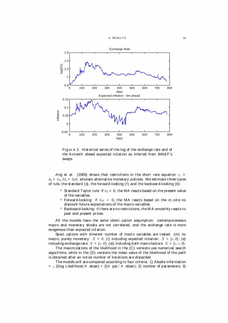
The expected in‡ation and the yield curve were extracted from contracts tradedon BM&F Bovespa. Our sample contains DIxPRE swap contracts with maturitiesf1, 2, 3, 6, 9, 12,18, 24, 36g-months, which represent the term structure, and INPCxDIswaps, which provide the di¤erence between the in‡ation rate measured by the con-sumer price index and the ‡oating interest rate observed at the contracted maturity.The ratio between the earnings of the latter asset and of the corresponding DIxPREswap was taken as a measure of the expected in‡ation for that maturity. However,this ratio contains a risk premium that was supposed constant and disregarded.We chose the 6-month ahead expected in‡ation. Our sample was determined bythe availability of those contracts at the time we collected the data, and it goesfrom April 2002 to October 2005, totaling 870 days. Figures 1 and 2 illustrate theevolution of the term structure and of the macro factors. As remarked in the intro-duction, it is di¢cult to …nd historical series that span many economic cycles in theBrazilian economy, because of the profound changes of regime that have occurreduntil recently.
Following Litterman and Scheinkman (1991), we analyzed the yield curve inBrazil, which indicated that 99% of the variance of the nine yield maturities inour sample can be described by two principal components (90% and 9% for the…rst and second component). This motivated us to …x two unobserved monetaryfactors. Then, the main sources of nominal shocks in the economy, the log of thenominal exchange rate and the expected in‡ation rate, were added. The indepen-dent structural shocks associated with those variables were identi…ed supposingthat the innovation of the exchange rate is more exogenous than the innovation ofexpected in‡ation, and zero correlation between the latent and observed shocks.Thus, the model has four independent exogenous shocks a¤ecting the short rate.
Summary statistics are given in Table A.In the A&P model, the relation between the short rate and the state variables is
interpreted as a reaction function of the MA to changes in the state of the economy(Taylor rule). In our model, speci…ed for a daily sample, this relation will alsore‡ect the market reaction to new information arriving continuously between theMA meetings to decide the benchmark rate, regarding future changes by the MAand macroeconomic values. Even though other market conditions in‡uence the

4. RE SULTS 17
short rate, the systematic reaction of the MA to shocks a¤ecting in‡ation and theexchange rate is contained in the impulse response function of the identi…ed shocks.
Table A. Summary statisticsCentral moments Autocorrelations
mean std dev skew kurt lag 21 lag 42 lag 631m 0.1961 0.0361 0.7789 2.2146 0.9524 0.8640 0.73722m 0.1975 0.0366 0.7195 2.1556 0.9458 0.8632 0.74803m 0.1990 0.0370 0.6570 2.0985 0.9403 0.8636 0.76096m 0.2034 0.0398 0.5898 2.0248 0.9196 0.8425 0.76659m 0.2070 0.0440 0.6654 2.0919 0.9040 0.8208 0.753612m 0.2104 0.0486 0.7671 2.2406 0.8998 0.8137 0.746318m 0.2168 0.0574 0.9009 2.4791 0.8973 0.8017 0.732924m 0.2227 0.0645 0.9586 2.5737 0.8973 0.7959 0.724836m 0.2330 0.0754 0.9973 2.6376 0.8945 0.7899 0.7149EX 1.0870 0.1100 0.3787 3.2437 0.7616 0.5721 0.3460in‡ation 0.0748 0.0311 -0.2446 3.0408 0.7991 0.6703 0.5394
Data description. The yield data is composed of daily rates obtained from the DIxPreswaps, provided by BM&F Bovespa, which approximates the Brazilian Government Bondszero-coupon constant maturity rates. The exchange rate series is provided by IPEADATA.The in‡ation data refers to a daily six-month ahead expected in‡ation series constructedusing the DIxPre and INPCxDI swaps. The table contains yield sample means, standarddeviations, skewness, kurtosis and autocorrelations. The sample period goes from April2002 to October 2005.
In the A&P model, the relation between the short rate and the state variables isinterpreted as a reaction function of the MA to changes in the state of the economy(Taylor rule). In our model, speci…ed for a daily sample, this relation will alsore‡ect the market reaction to new information arriving continuously between theMA meetings to decide the benchmark rate, regarding future changes by the MAand macroeconomic values. Even though other market conditions in‡uence theshort rate, the systematic reaction of the MA to shocks a¤ecting in‡ation and theexchange rate is contained in the impulse response function of the identi…ed shocks.
The identi…ed monetary factors have di¤erent characteristics. The unobservedfactor 1 is highly correlated to the di¤erence between the long and the short rate,and so we call it slope. The unobserved factor 2 is highly correlated to the meanvalue of the rates, and is denoted by level. This is shown in Tables 1 and 2. InRudebusch and Wu (2003), the estimated monetary factors show similar character-istics. Their model contains two unobserved monetary factors - slope and level -a MA reaction rule, and a transition equation derived from a “macro structural”model.
They interpreted the innovation that increases all the yield rates as a shockon the preferences of the MA with respect to the level of in‡ation, that is, as analteration of the in‡ation target. The innovation of the factor 2 was interpreted asan alteration of the monetary policy determinants, which could be caused by creditcrunches, price misalignments or increases of risk perception because of events likethe terrorist attack in the U.S. in 2001. In other words, it is an innovation thatis not linked to a movement of in‡ation, but rather to recurring …nancial marketcrises. An example in Brazil was the crisis preceding the presidential election in

181 . ASSESSING M AC RO INFLUENC E ON B RAZ IL IAN YIELD C URVE WIT H AFFINE M ODELS
0 100 200 300 400 500 600 700 80010
15
20
25
30
35
40
45
days
yiel
d in
%
1m2m3m6m9m12m18m24m36m
Figure 1. Evolution of the Brazilian domestic yield curve fromApril 2002 to October 2005.
2002, when local currency government bonds maturing after the election started tocarry a spread due to the perceived risk of default.
We now comment about numerical issues in the estimation process. In thelikelihood optimizations of (C) versions, lower dimensional models are estimated…rst and serve as initial points of other models. In the MCMC estimations of (D)versions, six chains are constructed and the one that presents the highest meanvalue of the log likelihood after convergence of the chain is chosen.
The analysis of the results includes three aspects: 1) the adherence, 2) thedegree of the interdependence among macro shocks and yields, and 3) the dynamice¤ect of the identi…ed shocks on the yield curve and on macro variables.
4.1. Evaluating Speci…cations. The inclusion of the macro variables andthe imposition of parameter restrictions will be considered, motivated by economicarguments or parsimony. Restrictions can be of two types: on the state variablestransition equation or on the short rate equation.
In the bilateral model (B), the dynamics of the latent variables and observedvariables are joined through the transition equation. The macro variables directlya¤ect the yield curve via the Taylor rule, or indirectly through the transition equa-tion. In the yield-to-macro unilateral model (U), the macro variables do not a¤ectthe transition of the latent variables (©θM = λθM = 0), but a¤ect them throughthe Taylor rule. This is the speci…cation estimated by A&P.
4. RE SULTS 19
0 100 200 300 400 500 600 700 8000.8
1
1.2
1.4
1.6
days
log(
EX
)
Exchange Rate
0 100 200 300 400 500 600 700 800-0.05
0
0.05
0.1
0.15
days
Expected Inflation - 6m ahead
Infla
tion
Figure 2. Historical series of the log of the exchange rate and ofthe 6-month ahead expected in‡ation as inferred from BM&F’sswaps.
Ang et al. (2005) shows that restrictions in the short rate equation rt =δ0 + δM Mt + δθθt emulate alternative monetary policies. We estimate three typesof rule, the standard (s), the forward-looking (f) and the backward-looking (b):
² Standard Taylor rule: if δθ = 0, the MA reacts based on the present valueof the variables.
² Forward-looking: if δM = 0, the MA reacts based on the in…nite nodiscount future expectations of the macro variables.
² Backward-looking: if there are no restrictions, the MA smoothly reacts topast and present prices.
All the models have the same identi…cation assumption: contemporaneousmacro and monetary shocks are not correlated, and the exchange rate is moreexogenous than expected in‡ation.
Speci…cations with di¤erent number of macro variables are tested: (m) nomacro, purely monetary: X = θ; (i) including expected in‡ation: X = (i, θ); (e)including exchange rate: X = (e,θ); (ei) including both macro factors: X = (e, i, θ).
The maximizations of the likelihood in the (C) versions use numerical searchalgorithms, while in the (D) versions the mean value of the likelihood of the pathis obtained after an initial number of iterations are discarded.
The models will are compared according to four criteria: 1) Akaike information= ¡2(log Likelihood/# obser) + 2(# par/ # obser); 2) number of parameters; 3)
201 . ASSESSING M AC RO INFLUENC E ON B RAZ IL IAN YIELD C URVE WIT H AFFINE M ODELS
0 500 1000
0.2
0.25
0.3
0.351m
0 500 10000.1
0.2
0.3
0.4
0.51y
0 500 1000
0.2
0.25
0.3
0.352m
0 500 1000
0.2
0.25
0.3
0.353m
0 500 10000.1
0.2
0.3
0.46m
0 500 10000.1
0.2
0.3
0.4
0.59m
0 500 10000.1
0.2
0.3
0.4
0.518m
0 500 10000.1
0.2
0.3
0.4
0.52y
0 500 10000.1
0.2
0.3
0.4
0.53y
days
DataModel
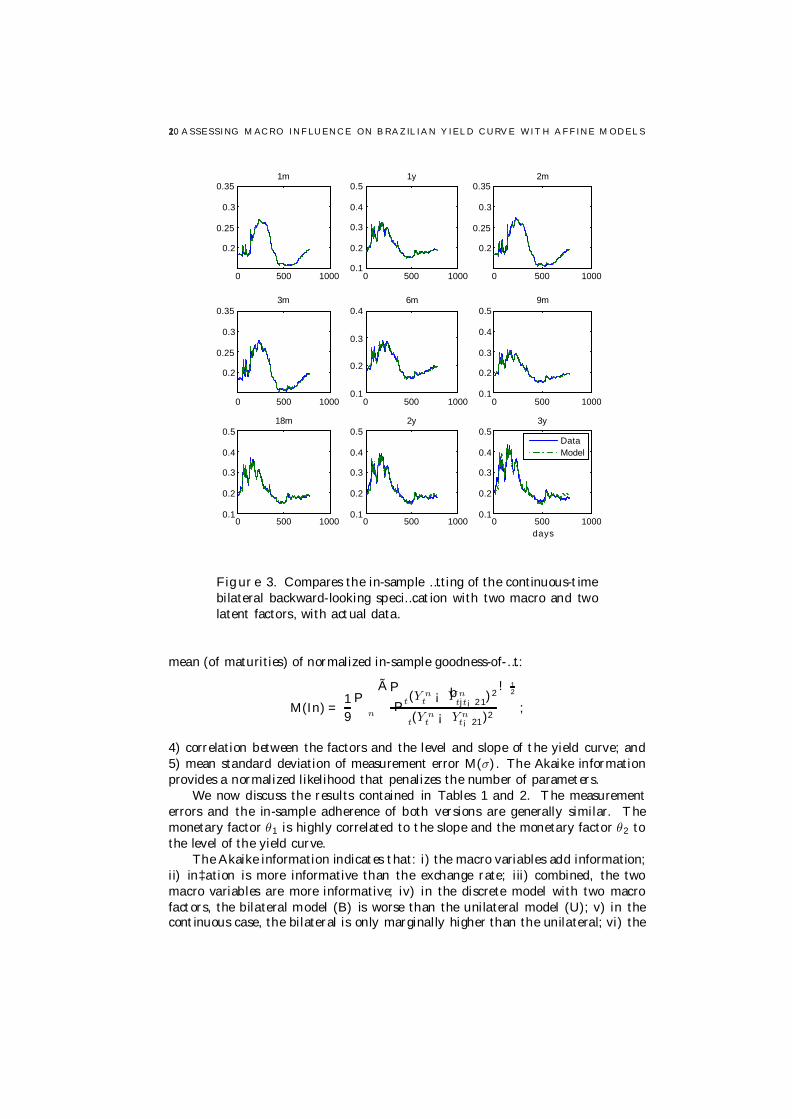
Figure 3. Compares the in-sample …tting of the continuous-timebilateral backward-looking speci…cation with two macro and twolatent factors, with actual data.
mean (of maturities) of normalized in-sample goodness-of-…t:
M(In) =19
Pn
ÃPt(Y n
t ¡ bY ntjt¡21)
2
Pt(Y n
t ¡ Y nt¡21)2
! 12
;
4) correlation between the factors and the level and slope of the yield curve; and5) mean standard deviation of measurement error M(σ). The Akaike informationprovides a normalized likelihood that penalizes the number of parameters.
We now discuss the results contained in Tables 1 and 2. The measurementerrors and the in-sample adherence of both versions are generally similar. Themonetary factor θ1 is highly correlated to the slope and the monetary factor θ2 tothe level of the yield curve.
The Akaike information indicates that: i) the macro variables add information;ii) in‡ation is more informative than the exchange rate; iii) combined, the twomacro variables are more informative; iv) in the discrete model with two macrofactors, the bilateral model (B) is worse than the unilateral model (U); v) in thecontinuous case, the bilateral is only marginally higher than the unilateral; vi) the

4. RE SULTS 21
standard rule restriction is the worst speci…cation, and the backward-looking thebest.
The models showed good …t in most of the speci…cations, as seen by themeasurement errors. Figure 3 compares the model implied yield curves of thecontinuous-time backward-looking version with the data.
Table 1: Comparison of discrete-time speci…cations.discrete Akaike #par M(In) C(θ1,slo) C(θ2,lev) M(σ)yields only -87 19 1.20 0.92 0.96 57backward-looking Taylor rule: in‡ation
unilateral -108 28 0.97 0.97 0.74 63bilateral -105 32 0.96 0.87 1.00 42
backward-looking Taylor rule: exchange rateunilateral -106 28 0.97 0.98 0.64 65bilateral -86 32 1.06 0.90 0.98 59
backward-looking Taylor rule: in‡ation, exchange rateunilateral -111 42 0.92 0.99 0.94 128bilateral -104 50 0.91 0.94 0.86 56
standard Taylor rule: in‡ation, exchange ratebilateral -84 48 1.35 0.90 0.86 175
forward-looking Taylor rule: in‡ation, exchange ratebilateral -98 48 1.41 0.87 0.98 56
Summary of results of the discrete-time model. The …rst line corresponds to a purelymonetary speci…cation and the others to speci…cations with in‡ation, exchange rate orboth, with unilateral or bilateral dynamics. The Taylor rule can be backward, standardor forward-looking. The columns show the Akaike information, the number of parameters,the mean over the maturities of the in-sample model …tting normalized by the randomwalk …tting, M(In), the correlation between the factors and the slope, C(θ1,slo), or thelevel, C(θ1,lev), of the yield curve, and the mean measurement errors in basis points,M(σ).
Table 2: Comparison of continuous-time speci…cationsdiscrete Akaike #par M(In) C(θ1,slo) C(θ2,lev) M(σ)yields only -90 17 0.96 0.90 0.68 45backward-looking Taylor rule: in‡ation
unilateral -101 26 0.95 0.92 0.9 42bilateral -101 30 0.94 0.83 0.88 42
backward-looking Taylor rule: exchange rateunilateral -99 26 0.97 0.93 0.85 44bilateral -99 30 0.95 0.70 0.86 43
backward-looking Taylor rule: in‡ation, exchange rateunilateral -109 40 0.94 0.85 0.63 37bilateral -110 48 0.92 0.55 0.89 40
standard Taylor rule: in‡ation, exchange ratebilateral -109 46 1.00 0.87 0.94 42
forward-looking Taylor rule: in‡ation, exchange ratebilateral -110 46 0.93 0.50 0.91 40
Summary of results of the continuous-time model, containing the same items as Ta-ble1.

221 . ASSESSING M AC RO INFLUENC E ON B RAZ IL IAN YIELD C URVE WIT H AFFINE M ODELS
4.2. Comparing Model Dynamics. The (C) and (D) versions describe theinteraction between the macro and the yield curve in distinct forms. As said before,in the continuous version some maturities are selected for the determination of thelatent factors and the dynamics is daily, while the discrete version is a monthlymodel de…ned based on daily data, in which the latent factors are obtained throughthe Kalman …lter. We consider in this subsection six speci…cations that includethe two macro factors to compare how the imposition of restrictions and choice ofversion alter the macro-yield interaction. All speci…cations were identi…ed consid-ering that macro and latent shocks are contemporaneously uncorrelated, and thatthe exchange rate is more exogenous than expected in‡ation.
The variance decomposition of the speci…cations is contained in Tables 3 and4. They show the proportion of the variance of the 18-month ahead forecast ofthe {1,9,36}-month yields and of the macro factors that are attributable to themonetary shocks and macro shocks, respectively.
In the unrestricted model, the macro variables a¤ect the yield curve directlythrough the Taylor rule, and indirectly through the state vector transition equation.The unilateral speci…cation eliminates the indirect channel, but the macro still af-fects the curve through the monetary policy channel. However, the decompositionof the yield movements of the backward-looking unilateral models showed no par-ticipation of the macro variables. This indicates that the macro-to-yield channeloccurs mainly through the transition equation.
Table 3: Variance decomposition of macro shocks 18 months aheaddiscrete unilateral backward bilateral backward bilateral forward
respnshock ex inf slo lev ex inf slo lev ex inf slo levex 77 3 20 0 24 55 11 9 60 3 37 0inf 3 58 16 23 3 81 14 3 2 32 63 31m 0 0 7 92 1 30 11 58 1 25 64 109m 0 0 23 77 2 45 16 37 0 10 85 53y 0 0 52 48 4 58 17 21 3 5 91 2
Variance decomposition of the exchange rate, in‡ation, and {1, 9, 36}-month yieldsusing the discrete-time versions with two macro factors, backward or forward-lookingTaylor rule and unilateral or bilateral dynamics. The lines contain the contributions ofthe exchange rate, in‡ation and latent factors.
Table 4: Variance decomposition of latent shocks 18 months aheaddiscrete unilateral backward bilateral backward bilateral forward
respnshock ex inf slo lev ex inf slo lev ex inf slo levex 31 05 55 10 77 04 19 00 78 3 19 00inf 03 40 53 05 21 64 14 00 22 64 14 001m 00 00 78 22 22 24 20 34 21 21 21 369m 00 00 96 04 21 07 40 33 20 07 38 353y 00 00 00 00 28 01 47 24 27 02 45 26
Variance decomposition of the exchange rate, in‡ation and {1, 9, 36}-months yieldsusing the continuous-time versions with two macro factors, backward or forward-lookingTaylor rule and unilateral or bilateral dynamics. The lines contain the contributions ofthe exchange rate, in‡ation and latent factors.
4. RE SULTS 23
Now, consider the second type of restriction, associated with the short rateformation. The forward- and backward-looking speci…cations show the same de-composition in the continuous case, while in the discrete case the e¤ect on macrovariables is roughly the same.
For the bilateral models, the in‡ation shock a¤ects the variance of the yields, inaccordance with the in‡ation target mechanism. Also, both versions show that themacro and latent variables are intertwined. Macro shocks impact the latent factorsand vice-versa. However, we remark that in the continuous version, the impact inthe macro-to-yield direction is greater, which is in accordance with Diebold et al.(2006).
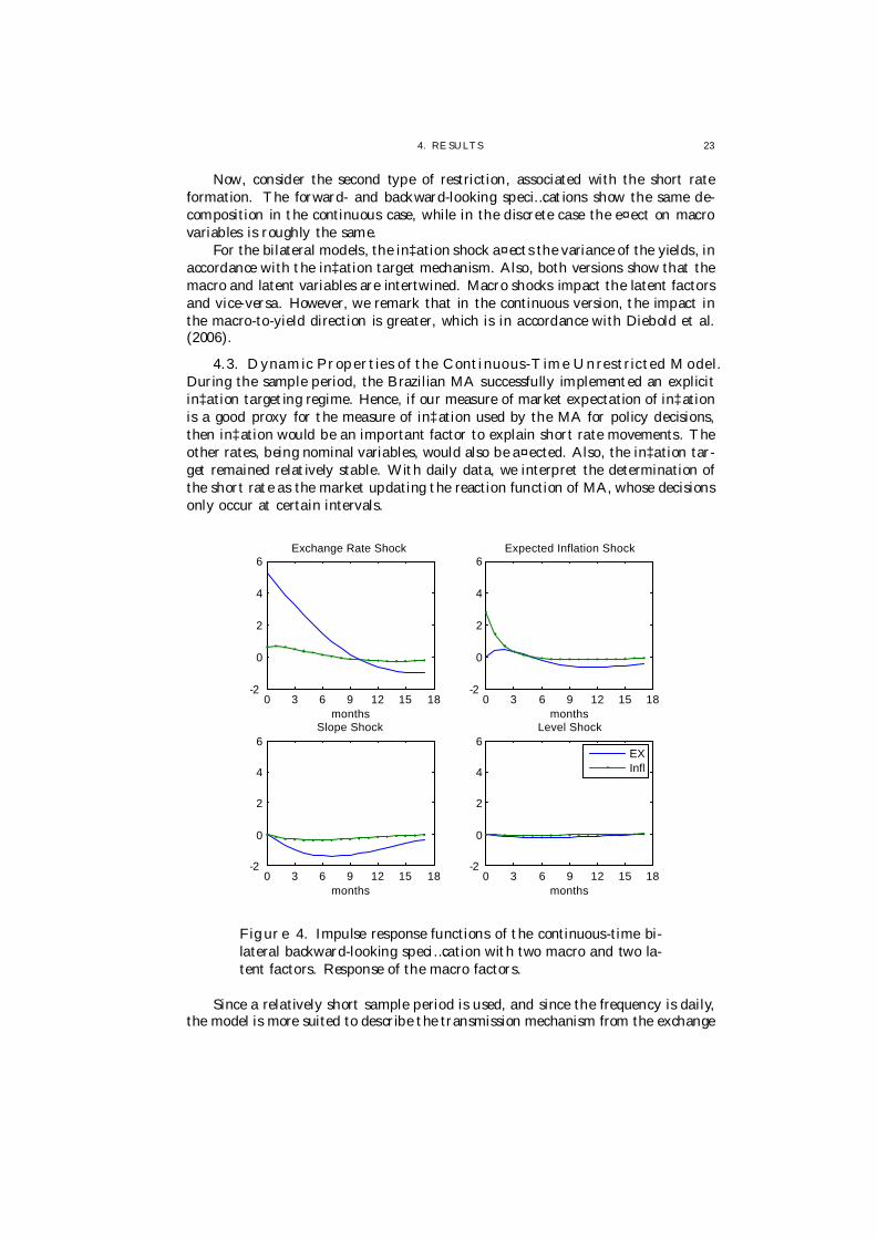
4.3. Dynamic Properties of the Continuous-Time Unrestricted Model.During the sample period, the Brazilian MA successfully implemented an explicitin‡ation targeting regime. Hence, if our measure of market expectation of in‡ationis a good proxy for the measure of in‡ation used by the MA for policy decisions,then in‡ation would be an important factor to explain short rate movements. Theother rates, being nominal variables, would also be a¤ected. Also, the in‡ation tar-get remained relatively stable. With daily data, we interpret the determination ofthe short rate as the market updating the reaction function of MA, whose decisionsonly occur at certain intervals.
0 3 6 9 12 15 18-2
0
2
4
6
months
Exchange Rate Shock
0 3 6 9 12 15 18-2
0
2
4
6
months
Expected Inflation Shock
0 3 6 9 12 15 18-2
0
2
4
6
months
Slope Shock
0 3 6 9 12 15 18-2
0
2
4
6
months
Level Shock
EXInfl
Figure 4. Impulse response functions of the continuous-time bi-lateral backward-looking speci…cation with two macro and two la-tent factors. Response of the macro factors.
Since a relatively short sample period is used, and since the frequency is daily,the model is more suited to describe the transmission mechanism from the exchange

241 . ASSESSING M AC RO INFLUENC E ON B RAZ IL IAN YIELD C URVE WIT H AFFINE M ODELS
0 3 6 9 12 15 18
-2
-1
0
1
2
months
Exchange Rate Shock
0 3 6 9 12 15 18
-2
-1
0
1
2
months
Expected Inflation Shock
0 3 6 9 12 15 18
-2
-1
0
1
2
months
Slope Shock
0 3 6 9 12 15 18
-2
-1
0
1
2
months
Level Shock
1m9m36m
Figure 5. Impulse response functions of the continuous-time bi-lateral backward-looking speci…cation with two macro and two la-tent factors. Response of yields.
rate and in‡ation to interest rates (and vice-versa) in the short run. We chose theunrestricted continuous-time model to analyze details of this transmission, avoidingunnecessary restrictions and focusing on one type of model. The variance decom-position for the forecasting horizons of one and nine months are given in Table5.
Table 5: Variance decomposition of the continuous-time versionH=1m H=9m
respnshock EX in‡ slope level EX in‡ slope levele 99 00 00 00 84 01 14 00i 09 91 00 00 18 70 12 00
1m 05 14 24 57 24 29 09 389m 14 20 13 53 07 10 41 4136m 17 03 39 41 11 02 58 30
Variance decomposition of the exchange rate, in‡ation and {1, 9, 36}-month yields.The model is the bilateral backward-looking continuous-time version with two macro fac-tors one and nine month horizons. Macro and latent shocks.
The results reveal that exchange rate shocks are important for the Brazilianeconomy, corresponding to roughly 20% of the variation of in‡ation and interestrates. The in‡ation shock corresponds to another roughly 20% of the variation ofthe interest rates. Thus, macro factors are responsible for roughly 40% of interest
4. RE SULTS 25
rate movements, a proportion that is lower than the A&P macro-to-yield modeland higher than the bilateral model of Diebold et al. (2006), both for the U.S.market. Ang et al. (2005) report a greater in‡uence of macro shocks on the spreadof the rates (long rate minus short rate), but they use only one latent variable. Ourestimation indicates that slope e¤ects, absent in single latent factor models, arevery important.
0 0.5 1 1.5 2 2.5 3-0.1
-0.05
0
0.05
0.1
0.15
0.2
0.25
0.3
years
Factor Loadings
EXInflLatent 1Latent 2
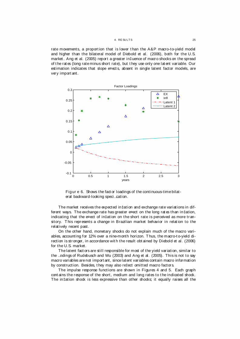
Figure 6. Shows the factor loadings of the continuous-time bilat-eral backward-looking speci…cation.
The market receives the expected in‡ation and exchange rate variations in dif-ferent ways. The exchange rate has greater e¤ect on the long rates than in‡ation,indicating that the e¤ect of in‡ation on the short rate is perceived as more tran-sitory. This represents a change in Brazilian market behavior in relation to therelatively recent past.
On the other hand, monetary shocks do not explain much of the macro vari-ables, accounting for 12% over a nine-month horizon. Thus, the macro-to-yield di-rection is stronger, in accordance with the result obtained by Diebold et al. (2006)for the U.S. market.
The latent factors are still responsible for most of the yield variation, similar tothe …ndings of Rudebusch and Wu (2003) and Ang et al. (2005). This is not to saymacro variables are not important, since latent variables contain macro informationby construction. Besides, they may also re‡ect omitted macro factors.
The impulse response functions are shown in Figures 4 and 5. Each graphcontains the response of the short, medium and long rates to the indicated shock.The in‡ation shock is less expressive than other shocks; it equally raises all the
261 . ASSESSING M AC RO INFLUENC E ON B RAZ IL IAN YIELD C URVE WIT H AFFINE M ODELS
rates and causes an initially upward and then downward impact on the exchangerate. The MA controls the short rate, but the long rate is formed in the market,suggesting that the market perceives that the rise is transitory.
The level shock raises all the nominal variables without changing the slope,as expected, followed by a smooth decrease over longer horizons. Indeed, if thein‡ation target regime works as an expectations organizer, than we would expecttarget changes to produce smooth rate changes.
The response to exchange rate shocks deeply alters the slope of the curve,raising the three-year yield, causing a strong but temporary e¤ect. The e¤ect onshort rate is more modest but more persistent, which reveals the type of responseof the MA.
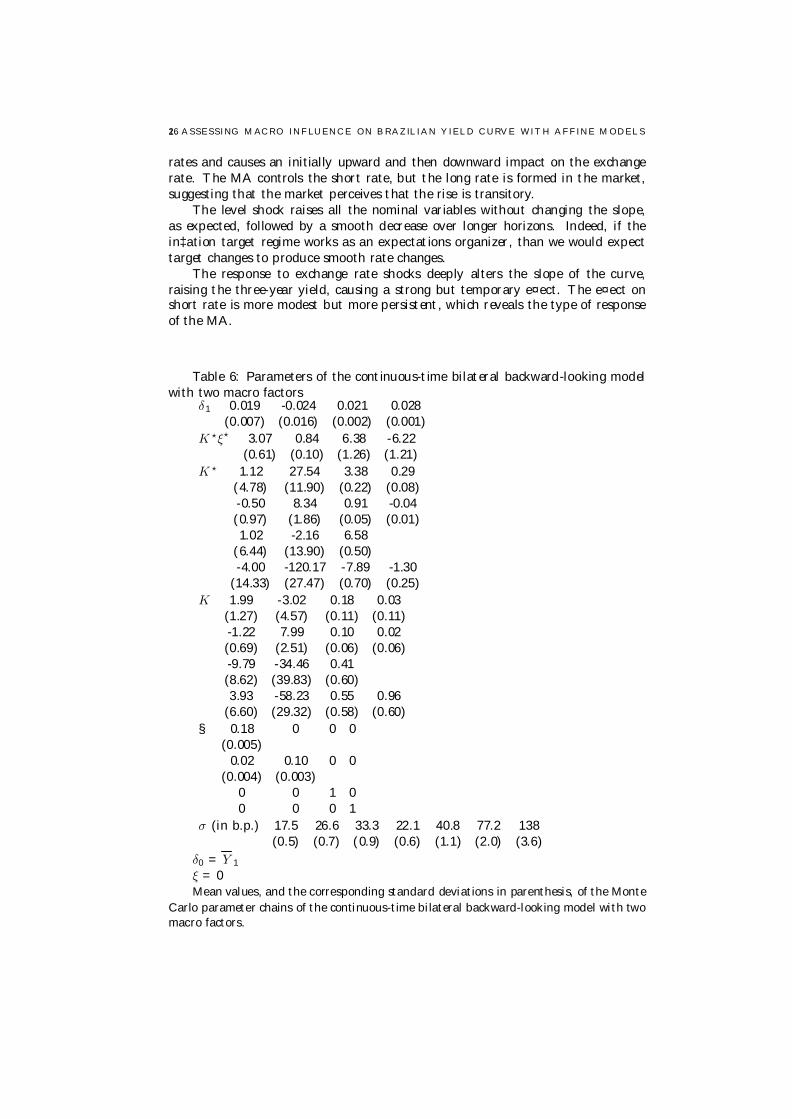
Table 6: Parameters of the continuous-time bilateral backward-looking modelwith two macro factors
δ1 0.019 -0.024 0.021 0.028(0.007) (0.016) (0.002) (0.001)
K ?ξ? 3.07 0.84 6.38 -6.22(0.61) (0.10) (1.26) (1.21)
K ? 1.12 27.54 3.38 0.29(4.78) (11.90) (0.22) (0.08)-0.50 8.34 0.91 -0.04(0.97) (1.86) (0.05) (0.01)1.02 -2.16 6.58
(6.44) (13.90) (0.50)-4.00 -120.17 -7.89 -1.30
(14.33) (27.47) (0.70) (0.25)K 1.99 -3.02 0.18 0.03
(1.27) (4.57) (0.11) (0.11)-1.22 7.99 0.10 0.02(0.69) (2.51) (0.06) (0.06)-9.79 -34.46 0.41(8.62) (39.83) (0.60)3.93 -58.23 0.55 0.96
(6.60) (29.32) (0.58) (0.60)§ 0.18 0 0 0
(0.005)0.02 0.10 0 0
(0.004) (0.003)0 0 1 00 0 0 1
σ (in b.p.) 17.5 26.6 33.3 22.1 40.8 77.2 138(0.5) (0.7) (0.9) (0.6) (1.1) (2.0) (3.6)
δ0 = Y 1ξ = 0Mean values, and the corresponding standard deviations in parenthesis, of the Monte
Carlo parameter chains of the continuous-time bilateral backward-looking model with twomacro factors.

5. CO NC LUSION 27
Finally, the e¤ects of the slope shock also strongly alter the slope of the yieldcurve, being responsible for most of the variation of the yields. Rudebusch andWu (2005) interpret this shock as a response to shocks not contained in the chosenmacro variables.
Factor loading - matrix B - represents the e¤ect of state variables along thematurities and is presented in Figure 6. The level factor loading, as expected, is‡at, and the slope factor loading decays over the maturities.
The parameter estimates of this section’s speci…cation and their standard errorsare given in Table 6.
5. Conclusion
This text follows the tradition of the …nance literature of using high-frequencydata to estimate a¢ne models with macro variables. Methodological questionsabout inference, choice of speci…cation of latent factors and ad hoc parameter re-strictions occurring in existing models motivated the consideration of a number ofversions of the model. One group of versions is speci…ed in continuous-time withdaily data, where latent factors are de…ned via Chen-Scott inversion, and estimatedusing maximum likelihood. Another group is speci…ed in discrete time with monthlydynamics, with factors extracted through the Kalman …lter, and estimated usingMCMC. We estimated three of the monetary policy speci…cations proposed by Anget al. (2005).
The models were used to analyze the Brazilian yield curve, which, because thecountry is an emerging market, has singular characteristics. The Brazilian economyevolved from a regime of high in‡ation and indexation up to 1994 to one of lowin‡ation under a new currency, with a …xed exchange rate regime (a “sliding peg”)that limited monetary policy options up to 1999, and then to an in‡ation targetingregime with a ‡oating exchange rate. This poses great challenges for the inferenceof the a¢ne models.
The main results are the following:(1) The exchange rate and the expected in‡ation improve the model’s capacity
to explain yield curve movements.(2) In spite of the cited di¤erences, the continuous and the discrete versions
show qualitatively similar results in most cases.(3) In general, restrictions on the number of parameters had a low e¤ect on the
adherence, but signi…cantly altered the dynamic properties of the model.Care must be taken in the use of arbitrary restrictions.
(4) An important part of the variance of the yields is due to monetary factorshocks, which do not allow a direct interpretation, but is related to thelevel and slope of the yield curve and may accommodate omitted macrovariables.
(5) The impulse response analysis showed that in‡ation shocks produce a tem-porary rise of moderate magnitude in the level, and exchange rate shocksproduce signi…cant changes in the slope of the curve, mostly through thelong-term yields.

CHAPTER 2
The Role of Macroeconomic Variables inDetermining Sovereign Risk
1. Introduction
Sovereign risk is a subtype of credit risk related to the possibility of a govern-ment failing to honor its payment obligations. It is a fundamental component ofemerging countries’ yield curves. Sovereign risk is also very important for emergingmarket …rms, since the cost of foreign …nancing typically rises with the country risk.Accordingly, the following questions are of particular interest: What are the factorsmost a¤ecting the sovereign yield curve? Which variables have greatest impact ondefault probabilities? This study presents an empirical investigation of these ques-tions by using an a¢ne term structure model with macroeconomic variables anddefault risk1.
There are two main approaches in credit risk modeling: structural and reducedform models2. While the former provides a link between the probability of defaultand …rms’ fundamental variables, the latter relies on the market as the only sourceof information regarding …rms’ credit risk structure. Black and Scholes (1973) andMerton (1974) proposed the initial ideas concerning structural models based onoptions theory. Black and Cox (1976) introduced the basic structural frameworkin which default occurs the …rst time the value of the …rm’s assets crosses a givendefault barrier. More recently, Leland (1994) extended the Black and Cox (1976)model, providing a signi…cant contribution to the capital structure theory. In hismodel, the …rm’s incentive structure determines the default barrier endogenously.That is, default is determined endogenously as the result of an optimal decisionpolicy carried out by equity holders.
All the papers cited above deal with the corporate credit risk case. However,the sovereign credit risk di¤ers markedly from corporate risk3. For instance, it isnot obvious how to model the incentive structure of a government and its optimaldefault decision, or what “assets” could be seized upon default. Moreover, post-default negotiating rounds regarding the recovery rate can be very complex anduncertain. Consequently, the use of structural models to assess the default risk ofa country is a delicate question. Not surprisingly, it is di¢cult to …nd studies of
1In this article, the term “macroeconomic (macro) variable” refers to any observable factor.2Giesecke (2004) provides a short introductory survey about credit risk models.3As discussed by Du¢e et al. (2003), the main di¤erences are: (i) A sovereign debt investor
may not have recourse to a bankruptcy code at the default event. (ii) Sovereign default can be apolitical decision. (iii) The same bond can be renegotiated many times. (iv) It may be di¢cultto collateralize debt with assets into the country. (v) The government can opt for defaulting oninternal or external debt. (vi) In the case of sovereign risk, it is necessary to take into account therole played by key variables such as exchange rates, …scal dynamics, reserves in strong currency,level of exports and imports, gross domestic product, and in‡ation.
29
302 . T HE ROLE O F M AC ROE CONOM IC VARIABLES IN DETE RM INING SOVEREIG N RISK
sovereign debt pricing based on the structural approach4 . Therefore, we opt to usereduced models, where the default time is a totally inaccessible stopping time thatis triggered by the …rst jump of a given exogenous intensity process5. This meansthat the default always comes as a “sudden surprise”, which provides more realismto the model. In contrast, within the class of structural models, the evolution ofassets usually follows a Brownian di¤usion, in which there are no such surprisesand the default time is a predictable stopping time.
Lando (1998), and Du¢e and Singleton (1999) develop versions of reducedmodels in which the default risk appears as an additional instantaneous spread inthe pricing equation. The spread can be modeled using state factors. In partic-ular, it can be incorporated into the a¢ne framework of Du¢e and Kan (1996),a widely used model o¤ering a good compromise between ‡exibility and numer-ical tractability6. Du¢e et al. (2003) extend the reduced model to include thepossibility of multiple defaults (or multiple “credit events”, such as restructuring,renegotiation or regime switches). The model is estimated in two steps. First,the risk-free reference curve is estimated. Next, the defaultable sovereign curve isobtained conditional on the …rst stage estimates. As an illustration, they applytheir model to analyze the term structure of credit spreads for bonds issued bythe Russian Ministry of Finance (MinFin) over a sample period encompassing thedefault on domestic Russian GKO bonds in August, 1998. They investigate thedeterminants of the spreads, the degree of integration between di¤erent Russianbonds and the correlation between the spreads and the macroeconomic variables.Another paper applying reduced model to emerging markets is Pan and Singleton(2008), who analyze the sovereign term structures of Mexico, Turkey, and Koreathrough a dynamic approach.
Nevertheless, Du¢e et al. (2003) and Pan and Singleton (2008) use a pure la-tent variables model. Thereby, the impact of macro factors changes on bond yieldscan be evaluated only indirectly through, for instance, a regression between observ-able and unobservable variables. Moreover, in pure latent models, the unobserv-able factors are abstractions that can, at best, be interpreted as geometric factorssummarizing the yield curve movements, as shown by Litterman and Scheinkman(1991).
The modern literature linking the dynamics of the term structure with macrofactors starts with Ang and Piazzesi (2003), who propose an ingenious solutionto incorporate observable factors in the original framework of a¢ne models. Intheir model, the macroeconomic factors a¤ect the entire yield curve. However, theinterest rates do not a¤ect the macroeconomic factors, which means that monetarypolicy is ine¤ective. Similarly to Du¢e et al. (2003), they employ a two-stepestimation procedure, …rst determining the macro dynamics and then the latentdynamics conditional on the macro factors. Ang et al. (2007) also combine macrofactors and no-arbitrage restrictions. Nevertheless, they use a Markov Chain MonteCarlo (MCMC) technique, which allows a single step estimation. On the other hand,Amato and Luisi (2006) estimate defaultable term structure models of corporate
4Exceptions are Xu and Ghezzi (2002) and Moreira and Rocha (2004).5A stopping time is totally inaccessible if it can never be announced by an increasing sequence
of predictable stopping times (see Schönbucher, 2003).6An a¢ne model is a multifactor dynamic term structure model, such that the state process
X is an a¢ne di¤usion, and the short short-term rate is also a¢ne in X

1. INT RO DUC T IO N 31
bonds with the inclusion of macroeconomic variables following a conditional three-step procedure: macro factors, then U.S. yield curve, and in the end corporatebonds.
Following the advances brought by these previous studies, we examine the im-pact of macro factors on a defaultable term structure through an a¢ne modelsimilar to that of Ang and Piazzesi (2003). We provide a comparison among avariety of speci…cations in order to determine the macro factors that most a¤ectcredit spreads and default probabilities of an emerging country. We also use impulseresponse and variance decomposition techniques to analyze the direct in‡uence ofobservable macro factors on yields and default probabilities.
However, before estimating the parameters, one must choose an identi…cationstrategy. Not all parameters of the multifactor a¢ne model can be estimated,since there are transformations of the parameter space preserving the likelihood.When sub-identi…ed, parameters can be arbitrarily rotated, while over-identi…edspeci…cations may distort the true response of the state variables. Based on the…ndings of Dai and Singleton (2000), we propose an identi…cation strategy for a¢nemodels with macro factors and default.
We select Brazil as the case study. The reason for this choice is that Brazil is oneof the most important emerging countries with a rich history of credit events7. Whenusing Brazilian data, one must take into account that frequent regime switches haveoccurred until recently, such as change from very high in‡ation to a stable economy(Real Plan, July 1994), change from …xed to ‡oating exchange rate in a currencycrisis in January 1999, and change of monetary policy to in‡ation targeting inJuly 1999. Thus, our sample comprises …ve and a half years of historical series.This sample size is compatible with that found in other recent academic studiescontaining data from emerging economies (see, for instance, Pan and Singleton,2008, and Almeida and Vicente, 2009). Furthermore, following these authors, wedecided to employ continuous-time modeling with high-frequency data in order toavoid small-sample biases.
Our main model contains …ve state variables: one latent factor for the referencedefault-free curve, one external macro factor, one internal macro factor, and twolatent factors for the Brazilian sovereign yield curve. We test the following observ-able variables: Fed interest rates, VIX (index of implied volatility of options inthe Standard & Poor’s index), Brazilian Real/US Dollar exchange rates, São PauloStock Exchange index (IBovespa), and Brazilian interest rate swaps. In the estima-tion stage we follow common practice and use a two-step procedure as implementedby Du¢e et al. (2003).
In a nutshell, we contribute to the international empirical …nance literature inat least two aspects. First, we extend the works of Du¢e et al. (2003) and Panand Singleton (2008) by incorporating macro variables in a dynamic term structuremodel with default risk. Second, our model allows a full interaction between latentand observable sovereign factors, which in a sense extends the study of Ang andPiazzesi (2003)8.
7Jointly with India, Russia and China, Brazil is considered as among the faster growingdeveloping economies in the world. Goldman Sachs refers to these countries as BRICs, an acronymthat means Brazil, Russia, India and China (see Goldman Sachs, 2007).
8Diebold et al. (2006), using a simple statistical model, …nd strong evidence of two-wayinteraction between latent and macro factors.

322 . T HE ROLE O F M AC ROE CONOM IC VARIABLES IN DETE RM INING SOVEREIG N RISK
Our main …ndings can be summarized as follows. First, VIX and Fed ratesstrongly a¤ect the default probabilities in the short and in the long term, respec-tively. Second, VIX has a great e¤ect on Brazilian sovereign yields, more than anyinvestigated domestic macro indicator. This result agrees with one of Pan and Sin-gleton’s (2008) conclusions that VIX has the most explanatory power for Mexicancredit default swap (CDS) spreads. Third, among the observable domestic factorsonly the slope of yield curve presents signi…cant explanatory power of the Braziliancredit risk spread. Finally, a latent factor highly correlated with the level of theBrazilian sovereign curve predicts a substantial fraction of the yield and defaultprobability movements. Since the Fed short rate has greater impact on the de-fault probabilities than Brazilian domestic short rate, our model suggests that U.S.monetary policy is more important to the Brazilian term structure of credit spreadsthan the Brazilian monetary policy. We also assert that volatility of internationalmarket (measured in our model by VIX) is more important to determine Brazilianspread than local conditions. On the other hand, the moderate signi…cance of thedomestic yield curve slope indicates that expectations of Brazilian investors playan important role in determining the sovereign yield and default probabilities.
The rest of this article is organized as follows. In Section 2 we present the model.Section 3 describes the dataset used. Section 4 details the estimation procedure.Section 5 presents the results of implementing the dynamic models. Section 6 o¤ersconcluding remarks.
2. A¢ne Model with Default Risk and Macro Factors
Uncertainty in the economy is characterized by a …ltered probability space(, (Ft)t¸0 , F, P) where (Ft)t¸0 is a …ltration generated by a standard N -dimensionalBrownian motion W P =
¡W P
1 , . . . , W PN
¢de…ned on (, F , P) (see Du¢e, 2001). We
assume the existence of a pricing measure Q under which discounted security pricesare martingales with respect to (Ft)t¸0. The price PD of a defaultable bond attime t that pays $1 at maturity time t + T is given by
(2.1) PD (t, T) = EQt
h1[τd>t+T ]e(¡
R t+Tt rudu) + Zτd1[τd·t+T ]e(¡
R t+Tt rudu)
i,
where 1A is the indicator function of the set A. The …rst part of the right-handside of (2.1) represents what the bondholder receives if the maturity time comesbefore the default time τd, a totally inaccessible stopping time. In case of default,the investor receives the random variable Zτd at the default time. Lando (1998),and Du¢e and Singleton (1999) prove that if τ d is doubly stochastic with intensityηt , the recovery upon default is given by Zτd = (1 ¡ `τd )PD (τd, T ), where `t is theloss rate in the market value, and if other technical conditions are satis…ed, then
(2.2) P D(t, T ) = EQt
"exp
á
Z t+T
t(ru + su)du
!#,
where st = `tηt is the spread due to the possibility of default.We now brie‡y explain the concept of doubly stochastic stopping time (for
more details, see Schönbucher, 2003 or Du¢e, 2001). De…ne N (t) = 1[τd·t]as the associated counting process. It can be shown that N (t) is a submartin-gale. Applying the Doob-Meyer theorem (see Shiryaev, 1995), we know there ex-ists a predictable, non-decreasing process C(t) called the compensator of N (t).One property of the compensator is to give information about the probabilities of

2. AFFINE MO DEL W IT H DE FAULT RISK AND M AC RO FAC TO RS 33
the jump time. The expected marginal increments of the compensator dC(t) areequal to the probability of the default occurring in the next increment of time:EQ
t [C (t + ¢t) ¡ C (t)] = Q [N (t + ¢t) ¡ N (t) = 1jFt ]. An intensity process ηt forN (t) exists if it is progressively measurable and non-negative, and C (t) =
R t0 η(u)du.
Under regularity conditions, it turns out that
(2.3) η (t) = lim¢t!0
1¢t
Q[τ d · t + ¢tjτd > t].
Thus, η(t) represents the evolution of the instantaneous probability of default-ing by t + dt if default has not occurred up to t. Finally, τd is said to be doublystochastic with intensity η if N (t2) ¡ N (t1)jη »Poisson
³R t2t1
η(u)du´. Therefore,
in the reduced model, the default event is essentially given by the …rst jump of aPoisson process with stochastic intensity.
Our model is within the class of a¢ne models analyzed by Du¢e and Kan(1996). The state vector Xt 2 RN incorporates information about the UnitedStates, XUS
t =³θUS
t , M USt
´, and Brazil, XBR
t =³MB R
t , θBRt
´, that is, Xt =
³θUS
t , MUSt , M BR
t , θBRt
´, where the variables θt =
³θUS
t , θBRt
´and Mt =
¡M US
t , MB Rt
¢
represent latent and observable factors, respectively. In the a¢ne model with de-fault, st and rt are speci…ed as a¢ne functions of the state vector. In other words,we assume that st = δs
0 + δs1 ¢ Xt and rt = δr
0 + (δr,US1 ,δr,BR
1 ) ¢ Xt = δr0 + δr
1 ¢ Xt,where δs
0, δr0 2 R and δs
1, δr1 2 RN . Then the default-adjusted short-rate process is
(2.4) Rt = R(Xt) = rt + st = δr0 + δs
0 + (δr1 + δs
1) ¢ Xt = δ0 + δ1 ¢ Xt .
The dynamics of the state variables is given by:
dXt =
2664
dθUSt
dMUSt
dM BRt
dθBRt
3775 =
26664
KUS ,USθ,θ 0 0 0
KUS ,USM,θ KUS ,US
M,M 0 0KB R,US
M,θ K BR ,USM,M K BR ,BR
M,M KB R,BRM,θ
KB R,USθ,θ K BR ,US
θ,M K BR ,BRθ,M KB R,BR
θ,θ
37775
0BB@
2664
ξUSθ
ξUSM
ξBRM
ξBRθ
3775 ¡
2664
θUSt
M USt
MBRt
θB Rt
3775
1CCA dt
+
26664
§US ,USθ,θ 0 0 0
§US ,USM,θ §US ,US
M,M 0 0§B R,US
M,θ §BR ,USM,M §B R,BR
M,M 0§B R,US
θ,θ §BR ,USθ,M §B R,BR
θ,M §B R,BRθ,θ
37775
2664
dW P,USθ (t)
dW P,USM (t)
dW P,B RM (t)
dW P,B Rθ (t)
3775
= K(ξ ¡ Xt)dt + §dW P(t),(2.5)
where K and § are N £N matrices and ξ 2 RN . That is, X follows an a¢ne processwith constant volatility. Similar to Du¢e et al. (2003), we set a “block-triangular”form for the dynamics of the state variables. The zeros above the main diagonalof § and K imply that the American yield curve factors a¤ect the Brazilian yieldcurve factors, but not vice versa. Furthermore, unlike Ang and Piazzesi (2003), weallow the macro and yield factors to interact fully.
The connection between martingale probability measure Q and objective prob-ability measure P is given by Girsanov’s Theorem with a time-varying risk premium:

342 . T HE ROLE O F M AC ROE CONOM IC VARIABLES IN DETE RM INING SOVEREIG N RISK
(2.6) dW Pt = dWQ
t ¡ (λ0 + λ1Xt)dt,
where λ0 =³λUS
0 , λB R0
´2 RN and λ1 is N £ N matrix given by
λ1 =·
λUS,US1 0
λBR ,US1 λB R ,BR
1
¸
As a result, the price PB R of a defaultable bond is exponential a¢ne, that is,PB R(t, T ) = exp
¡aBR(τ) + bBR (τ)X t
¢, where τ = T ¡ t, and aB R and bB R solve a
system of Riccati di¤erential equations:
bB R(τ)0 = ¡(δr1 + δs
1) ¡ K?0bB R(τ)
aB R(τ)0 = ¡(δr0 + δs
0) + ξ?0K?0bBR (τ) +12bBR (τ)0§§0bBR (τ),(2.7)
with K? = K +§λ1 and ξ? = K?¡1(Kξ ¡§λ0). An explicit solution for this systemof di¤erential equations exists only in some special cases, such as diagonal K.However, the Runge-Kutta method provides accurate numerical approximations.Thus, the yield at time t with time to maturity τ is given by
(2.8) Y BRt (τ) = ABR (τ) + BB R,US
θ (τ)θUSt +
BB R,USM (τ)MUS
t + BB R,BRM (τ)MBR
t + BBR ,BRθ (τ)θBR
t .
If the loss given default rate is constant, i.e. `t = ` for all t, then the termstructure of default probabilities is given by (see Schönbucher, 2003):
(2.9) Pr(t, T ) = 1 ¡ EPt
"exp
á
Z t+T
t
su
`du
!#,
which can be calculated similarly to the conditional expectation contained in thepricing equation, with the ob jective measure replacing the martingale measure. Itturns out that Pr(t, τ) = 1 ¡ exp(aPr(τ) + bPr(τ)Xt), where aPrand bPr are againsolutions of Riccati di¤erential equations:
bPr 0(τ) = ¡δs1/` ¡ K 0bPr(τ ),(2.10)
aPr 0(τ) = ¡δs0/` + ξ0K 0bPr(τ ) +
12bPr(τ)0§§0bPr(τ).
We close this section with two remarks. First, the reduced model can be re-placed by a standard term structure model with macro factors: it su¢ces to let theUS factors take the role of macro factors for the defaultable bonds. However, theinterpretation of the spread as the instantaneous expected loss and the computationof model implied default probabilities are no longer possible. Second, all the modelsin this article are in the class of Gaussian models, the simplest speci…cation of thea¢ne family. The inclusion of macro variables and default substantially compli-cates the model and its estimation. Therefore, we decided not to use a model withstochastic volatility. However, note that macro factors such as the VIX volatilitycan approximately play the role of stochastic volatility of the non-Gaussian a¢nemodels. Furthermore, models with constant volatility are the best choice matchingsome stylized facts (as shown, for instance, by Du¤ee, 2002, and Dai and Singleton,2002) and to describe corporate CDS spreads (see Berndt et al., 2004).

3. DATA 35
2.1. Impulse Response and Variance Decomposition. One way to eval-uate the impact of macro shocks on the term structure of interest rates and defaultprobabilities is through impulse response functions (IRF) and variance decomposi-tions (VD).
The response of the yield Yt = A + BXt is given by(2.11)
B§p
¢tεt Be¡K¢t§p
¢tεt Be¡2K¢t§p
¢tεt Be¡3K¢t§p
¢tεt ...t + 0 t + 1 t + 2 t + 3 ...
and the response of the logarithm of the survival probability, log Pr(t, τ) = aPr +bPrXt, is(2.12)
bPr§p
¢tεt bPre¡K¢t§p
¢tεt bPre¡2K¢t§p
¢tεt bPre¡3K¢t§p
¢tεt ...t + 0 t + 1 t + 2 t + 3 ...
Moreover, the contribution corresponding to the jth factor in the variance de-composition of Yt+h(τ) and log Prt+h(τ) at time t are
(2.13)V Dj (Y ) = B 0(τ)
³R t+ht e¡K (t+h¡u)§j§0
j (e¡K (t+h¡u))0du´
B(τ ),
V Dj (log) = bPr0(τ )³R t+h
t e¡K (t+h¡u)§j§0j(e¡K(t+h¡u))0du
´bPr(τ ).
3. Data
Our sample consists of a daily series of the following variables: (i) constantmaturity zero-coupon term structure of U.S. yields provided by the Federal Reserve(Fed); (ii) constant maturity zero-coupon term structure of Brazilian sovereignyields constructed by Bloomberg9; (iii) the implied volatility of S&P 500 indexoptions measured by the Chicago Board Options Exchange Volatility Index - VIX;(iv) Brazilian Real/US Dollar exchange rate, (v) São Paulo Stock Exchange index- IBovespa1 0, (vi) Brazilian domestic zero coupon yields extracted from DI x Preswaps obtained from Brazilian Mercantile and Futures Exchange (BM&F)11 . The…rst two data set are used as basic yields and the others take the role of observed(macro) factors in our model.
The sample begins on February 17, 1999, and ends on September 15, 2004, witha total of 1320 days. The sample starts one month after the change of the exchangerate regime from …xed to ‡oating in January 1999, forced by a devaluation crisis.The maturities of the US and Brazilian sovereign yields are the same, namely 3 and 6months, 1, 2, 3, 5, 7, 10, and 20 years while the maturities of the Brazilian domesticyields are 1, 3, and 36 months. Figure 1 depicts the US and Brazilian sovereignyields. Figure 2 shows the observed variables. Note that the American yield curve isalmost ‡at in the beginning of the sample. After January 2001, short-yields declineover time and the shape of the term structure changes to upward sloping. In endof 2002, there is a stress movement in the Brazilian market due to a presidentialsuccession process in which the candidate of the opposition won the election.
9The dataset of sovereign yields provided by Bloomberg is extracted from Brazilian Globalbonds.
10Ibovespa is the main Brazilian stock market index.11The ID rate is the average one-day interbank borrowing/lending rate, calculated by CETIP
(Center of Custody and Financial Settlement of Securities) every business day. The ID rate isexpressed in e¤ective rate per annum, based on 252 business-days.
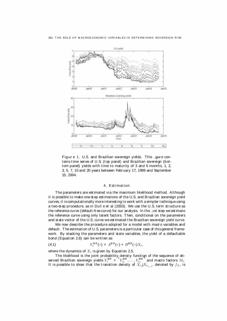
362 . T HE ROLE O F M AC ROE CONOM IC VARIABLES IN DETE RM INING SOVEREIG N RISK
Figure 1. U.S. and Brazilian sovereign yields. This …gure con-tains time series of U.S. (top panel) and Brazilian sovereign (bot-tom panel) yields with time to maturity of 3 and 6 months, 1, 2,3, 5, 7, 10 and 20 years between February 17, 1999 and September15, 2004.
4. Estimation
The parameters are estimated via the maximum likelihood method. Althoughit is possible to make one-step estimations of the U.S. and Brazilian sovereign yieldcurves, it is computationally more interesting to work with a simpler technique usinga two-step procedure, as in Du¢e et al (2003). We use the U.S. term structure asthe reference curve (default-free curve) for our analysis. In the …rst step we estimatethe reference curve using only latent factors. Then, conditional on the parametersand state vector of the U.S. curve we estimated the Brazilian sovereign yield curve.
We now describe the procedure adopted for a model with macro variables anddefault. The estimation of U.S. parameters is a particular case of this general frame-work. By stacking the parameters and state variables, the yield of a defaultablebond (Equation 2.8) can be written as
(4.1) Y B Rt (τ) = AB R(τ ) + BBR(τ)Xt ,
where the dynamics of Xt is given by Equation 2.5.The likelihood is the joint probability density function of the sequence of ob-
served Brazilian sovereign yields Y BRt =
¡Y BR
t1 , . . . , Y BRtn
¢and macro factors Mt.
It is possible to show that the transition density of Xti jXti¡1 , denoted by fX , is

4 . EST IMAT ION 37
Figure 2. Observable variables. This …gure contains time seriesof variables used as observable factors in our model between Febru-ary 17, 1999 and September 15, 2004. The upper left panel showsthe evolution of the VIX (implied volatility of S&P 500 index op-tions). The upper right panel presents the logarithm of the Brazil-ian Real/US Dollar exchange rate. The left lower panel presentsthe logarithm of the Ibovespa (São Paulo Stock Exchange index),and the right lower panel shows the Brazilian domestic zero-couponyields with time to maturity of 1, 3 and 36 months.
normally distributed with mean µB Ri = e¡K(ti¡ti¡1)Xti¡1 +
³IN ¡ e¡K(ti¡ti¡1)
´ξ
and variance (σBRi )
2=
Z ti
ti¡1
e¡K (ti¡u)§§0e¡K(ti¡u) 0du (see, for instance, Fackler,
2000).Suppose …rst the vectors θBR
t and Y BRt have the same dimension, that is, we
observe as many yields as latent variables. Then, we can invert a linear equationand …nd the unobserved factors θB R
t as a function of yields Y BRt and observable
factors MB Rt . Using change of variables, the log-likelihood function can be written
as
L(Yt , Mt, ª) =HX
t=2
logfX (XtjXt¡1, ª) + (H ¡ 1)log det jJacj,

382 . T HE ROLE O F M AC ROE CONOM IC VARIABLES IN DETE RM INING SOVEREIG N RISK
where H is the sample size, ª = (δ0, δ1, K, ξ, §, λ0, λ1) is a vector stacking themodel parameters, and the Jacobian matrix is
(4.2) Jac = ¹BBR (τ1, . . . , τN BR ) =
264
BB R(τ 1)...
BBR(τNBR )
375 ,
where τ 1, . . . , τN BR are the time to maturities of the observable Brazilian yields.If we want to use additional yields, direct inversion is not possible. This is
known as “stochastic singularity”. One solution is to follow Chen and Scott (1993),and add measurement errors to the extra yields. Let NB R
obs be the number of Brazil-ian sovereign yields observed on each day, NBR
obs > NB R where NB R is the size ofXBR
t . We select NB R yields to be priced without error. The other (NBRobs ¡NBR ) are
priced with independent normal measurement errors. Therefore, the log-likelihoodfunction is
L(Yt , Mt, ª) =HX
t=2
logfX (XtjXt¡1, ª) + (H ¡ 1)log det jJacj +12
HX
t=2
u0t
¡1ut,
where ut is the vector of yield measurement errors and represents the covariancematrix for ut , estimated using the sample covariance matrix of the ut ’s implied bythe extracted state vector, and Jac = ¹BB R(τ 1, ¢ ¢ ¢ , τ NBR
obs).
In order to complete the estimation procedure, it is necessary to identify themodel. If the model is sub-identi…ed then there are more than one set of parametersthat generate the same likelihood. Therefore, not all parameters can be estimated.On the other hand over-identi…ed models produce sub-optimal results that maydistort the impulse response functions. However, identi…cation of parameters ina state-space system is tricky. In the next subsection, we provide identi…cationstrategies for some speci…cations of our model based on the results of Dai andSingleton (2000).
4.1. Model Identi…cation. Here, we show how to identify the parameters ofa Gaussian a¢ne model with macro factors and credit spreads. This approach isbased on the study of Dai and Singleton (2000).
First we consider the default-free case. Suppose there are p macro variables Mand q latent variables θ. The vector X = (M,θ) follows a Gaussian a¢ne dynamics:
dXt =·
dMtdθt
¸=
·KM,M KM,θKθ,M Kθ,θ
¸ µ·ξMξθ
¸¡
·Mtθt
¸¶dt
+·
§M,M §M,θ§θ,M §θ,θ
¸ ·dW P
M(t)dW P
θ (t)
¸= K(ξ ¡ Xt)dt + §dW P(t).(4.3)
The instantaneous short-term rate is given by rt = δ0+δ1 ¢Xt while the market priceof risk obeys Equation 2.6. Hence, the dynamics of X in the risk-neutral measureis dX = K?(ξ? ¡ Xt)dt + §dW Q(t) and the yield curve is an a¢ne function of X ,Yt(τ ) = A(τ) + BM (τ)Mt + Bθ
t (τ )θ = A(τ) + B(τ)Xt . The parameter vector isdenoted by ª = (δ0, δ1, K, ξ, λ0, λ1, §).
Some of the above parameters must be arbitrarily …xed, otherwise there aremultiple solutions to the estimation problem since we can de…ne operators thatpreserve the likelihood as shown below.

4 . EST IMAT ION 39
Let L 2 R(p+q)£(p+q) be a non-singular matrix and v 2 Rp+q a vector such that
L =µ
I 0α β
¶and v =
µ0vθ
¶,
where I 2 Rp£p is the identity matrix, α 2 Rq£p, β 2 Rq£q , and vθ 2 Rq . Considerthe following maps:(4.4)
TL,vfª, Xg =f(δ0 ¡ δ0
1L¡1v, (L0)¡1δ1, LKL¡1, v + Lξ, λ0 ¡ λ1L¡1v, λ1L¡1, L§), LX + vg
and
(4.5) TOfª, Xg = f(δ0, δ1, K,ξ, λ0,λ1, §O0), Xg,
where O 2 R(p+q )£(p+q) is a rotation matrix.
Proposition 1. The operators TL,v and TO preserve the likelihood of the a¢nemodel de…ned above under the Chen-Scott (1993) estimation procedure.
ProofThe log-likelihood L of the a¢ne model under the Chen-Scott (1993) inversion
is
L(ª, X) = logfY (Yt1 , ..., YtH jª, X) =logfX (Xt1 , ..., XtH jª) + logfu(ut1,...,utH) + logj detJacjH ¡1 =(H ¡ 1)logj det ¹Bθ j +
PHt=2 logfXtjXt¡1(Xt jª) + logfu(ut) =
(H ¡ 1)logjdet ¹Bθ j ¡ 12 (H ¡ 1)log det
h¢t
¡e¡K¢t
¢§§0¡e¡K¢t
¢0i
+PH
t=2 logfu(ut) ¡ 12
PHt=2(Xt ¡ µ)0
h¢t
¡e¡K¢t
¢§§0¡e¡K¢t
¢0i¡1(Xt ¡ µ),
where µ = e¡K¢tξ +(1¡ e¡K¢tξ)Xt¡1, ¢t = ti ¡ ti¡1 8i, H is the sample size, and¹Bθ(¢) is evaluated at the time to maturities of yields without measurement errors(see Equation 4.2).
We begin by proving that L(ª, X) = L(TL,v (ª, X)). The strategy of the proofis to analyze what happens with each of the four terms of the log-likelihood when theoperator TL,v is applied. First, note that the expression under the last summationsymbol is preserved. The transformation of µ is
µ(TL,v(ª, X)) = e¡LKL¡1¢tLξ +³1 ¡ e¡LKL¡1¢t
´LXt¡1 =
Le¡K¢tL¡1Lξ + (1 ¡ Le¡K¢tL¡1)LXt¡1 = Lµ.
Then, applying TL,v on the last summation expression of the log-likelihood, we have
(LXt ¡ Lµ)0·³
e¡LKL¡1¢tL§p
¢t´ ³
e¡LKL¡1¢tL§p
¢t´0¸¡1
(LXt ¡ Lµ) =
(Xt ¡ µ)0L0·³
Le¡K¢tL¡1L§p
¢t´ ³
Le¡K¢tL¡1L§p
¢t´0¸¡1
L(Xt ¡ µ) =
(Xt ¡ µ)0L0·L0¡1
³e¡K¢t§
p¢t
´0¡1 ³e¡K¢t§
p¢t
´¡1L¡1
¸L(Xt ¡ µ) =
(X t ¡ µ) 0·³
e¡K¢t§p
¢t´0¡1 ³
e¡K¢t§p
¢t´¡1
¸(Xt ¡ µ).
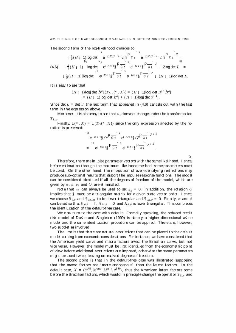
402 . T HE ROLE O F M AC ROE CONOM IC VARIABLES IN DETE RM INING SOVEREIG N RISK
The second term of the log-likelihood changes to
(4.6)
¡ 12 (H ¡ 1)log det
·³e¡LKL¡1¢tL§
p¢t
´ ³e¡LKL¡1¢tL§
p¢t
´0¸=
¡ 12 (H ¡ 1)
½log det
·³e¡K¢t§
p¢t
´ ³e¡K¢t§
p¢t
´0¸+ 2log detL
¾=
¡ 12 (H ¡ 1)[log det
·³e¡K¢t§
p¢t
´ ³e¡K¢t§
p¢t
´0¸¡ (H ¡ 1)log det L.
It is easy to see that
(H ¡ 1)logj det ¹Bθ j (TL,v(ª, X)) = (H ¡ 1)logj det β¡1 ¹Bθ j= (H ¡ 1)logj det ¹Bθ j + (H ¡ 1)logj detβ¡1j.
Since detL = det β, the last term that appeared in (4.6) cancels out with the lastterm in the expression above.
Moreover, it is also easy to see that ut does not change under the transformationTL,v.
Finally, L(ª, X) = L(TO(ª, X)) since the only expression a¤ected by the ro-tation is preserved:
·³e¡K¢t§O0p¢t
´ ³e¡K¢t§O0p¢t
´0¸¡1
=·³
e¡K¢t§p
¢t´ ³
e¡K¢t§p
¢t´0¸¡1
.
2Therefore, there are in…nite parameter vectors with the same likelihood. Hence,
before estimation through the maximum likelihood method, some parameters mustbe …xed. On the other hand, the imposition of over-identifying restrictions mayproduce sub-optimal results that distort the impulse response functions. The modelcan be considered identi…ed if all the degrees of freedom of the model, which aregiven by α, β, vθ and O, are eliminated.
Note that vθ can always be used to set ξθ = 0. In addition, the rotation Oimplies that § must be a triangular matrix for a given state vector order. Hence,we choose §θ,θ and §M,M to be lower triangular and §M,θ = 0. Finally, α and βcan be set so that §θ,θ = I , §M,θ = 0, and Kθ,θ is lower triangular. This completesthe identi…cation of the default-free case.
We now turn to the case with default. Formally speaking, the reduced creditrisk model of Du¢e and Singleton (1999) is simply a higher-dimensional a¢nemodel and the same identi…cation procedure can be applied. There are, however,two subtleties involved.
The …rst is that there are natural restrictions that can be placed to the defaultmodel coming from economic considerations. For instance, we have considered thatthe American yield curve and macro factors a¤ect the Brazilian curve, but notvice versa. However, the model must be …rst identi…ed from the econometric pointof view before additional restrictions are imposed, otherwise the same parametersmight be …xed twice, leaving unresolved degrees of freedom.
The second point is that in the default-free case was illustrated supposingthat the macro factors are “more endogenous” than the latent factors. In thedefault case, X = (θUS, MUS , MB R , θB R), thus the American latent factors comebefore the Brazilian factors, which would in principle change the operator TL,v and

5. RE SULTS 41
consequently the degrees of freedom. The other inversion, namely the Americanmacro vector coming after the latent vector, is due to the fact that only the VIX isconsidered and it does not interfere with the identi…cation procedure.
However, since we use a two-step procedure, the parameters and state factorsrelated to the American term structure are estimated …rst. So, we can think ofthe American latent factors as if they were “macro” factors and proceed to theidenti…cation considering that fMBR = (θUS , MUS, M BR) is in fact the macro vectorfor the default case.
In summary, the economic restrictions impose that δr1 = (δr,US
1 , 0) and thatthe matrix K is block-triangular, which means that Brazilian factors do not a¤ectAmerican factors. Therefore the identi…ed § is given by:
µ e§MM 00 I
¶, where e§MM =
0@
I 0 00 §US ,US
M,M 0§B R ,US
M,θ §BR ,USM,M §B R ,BR
M,M
1A .
5. Results
In this section we analyze the results of three di¤erent speci…cations of ourmodel estimated by the maximum likelihood method described in Section 4. Webegin with a simple macro-to-yield without default speci…cation. In order to avoidlocal maxima, many trial numerical optimizations are performed using the Nelder-Mead Simplex algorithm until stable results are obtained. Then, taking advantageof these results, we select starting vectors for the estimation of two higher di-mensional models with default. After that, other independent trial maximizationstarting from random vectors are performed. Finally we choose the best results.Although this procedure may be path-dependent, the “curse of dimensionality”does not allow the use of a complete grid of random starting points as would bedesirable.
5.1. Macro-to-yield without default. The simplest speci…cation of ourmodel is characterized by a macro-to-yield dynamics without default. It is ex-actly the model of Ang and Piazzesi (2003) applied to the Brazilian yield curve.The absence of default implies that American latent factors (θUS) are unnecessary.In a macro-to-yield model the observable factors a¤ect the latent factors but notvice versa. This means that KBR ,B R
M,θ is a matrix of zeros.The macro-to-yield without default speci…cation presents three state variables,
X = (M, θBR1 , θB R
2 ). It serves to indicate the relevant macro factors for the sovereignyield curve, which are then selected for use in the other models. To extract Brazilianlatent factors, we set the 3-month and 5-year sovereign yields to be ‡awless. Nineversions are estimated, each having a di¤erent observed factor M : (1) VIX; (2)logarithm of the Brazilian Real/US Dollar exchange rate (LEX); (3) logarithm ofthe IBovespa (LIBOV); (4) BM&F 1-month yield (B1m); (5) BM&F 3-year yield(B3y); (6) BM&F slope (Bsl) = B3y - B1m; (7) Fed 1-month yield (F1m); (8) Fed10-year yield (F10y), and (9) Fed slope (Fsl)= F10y - F1m.
Table 1 presents the log-likelihood divided by the number of observations (L/H)and the mean (for the nine maturities) of the absolute measurement errors in basispoints (MAE) for all speci…cations. These measures can be used to evaluate thedi¤erent versions of a model. Table 1 also presents the correlations between factor

422 . T HE ROLE O F M AC ROE CONOM IC VARIABLES IN DETE RM INING SOVEREIG N RISK
1 (θBR1 ) and the slope of the Brazilian sovereign term structure (ρ1,s) and between
factor 2 (θB R2 ) and the level of the Brazilian sovereign term structure (ρ2,l). The
likelihood does not vary signi…cantly, but the speci…cations that included US ratesshow slightly higher values. The mean absolute measurement error is around 60basis points. The latent factor θB R
2 represents the level, since it is highly correlatedwith this factor in all cases, while θBR
1 can be interpreted as the slope due to itspositive correlation with the slope of the yield curve.
Table 1. Summary of results of the macro-to-yield without de-fault model.
VIX LEX LIBOV B1m B3y Bsl F1m F10y FslL/H 44.7 44.3 44.3 44.8 44.8 45.0 47.5 47.5 47.1ρ1,s 0.20 0.37 0.29 0.59 0.56 0.57 0.66 0.69 0.61ρ2,l 0.99 0.83 0.98 0.94 0.94 1.00 0.94 0.84 0.94
MAE 54 66 56 62 62 58 62 61 62
This table presents the log-likelihood divided by the number of observations (L/H), themean (for the nine maturities) of the absolute measurement errors in basis points (MAE),and the correlations between factor 1 (θB R
1 ) and the slope of the Brazilian sovereign yieldcurve (ρ1,s) and between factor 2 (θBR
2 ) and the level of the Brazilian sovereign yield curve(ρ2,l). The macro-to-yield without default model presents only one observable factor ineach speci…cation. They are (1) VIX; (2) logarithm of the BR Real/US Dollar exchangerate (LEX); (3) logarithm of the Ibovespa (LIBOV); (4) BM&F 1-month yield (B1m);(5) BM&F 3-years yield (B3y); (6) BM&F slope (Bsl) = B3y - B1m; (7) Fed 1-monthyield (F1m); (8) Fed 10-years yield (F10y), and (9) Fed slope (Fsl)= F10y - F1m.
In order to measure the relative contributions of the macro and latent factorsto forecast variances we perform variance decompositions. Table 2 presents theproportion of the 1-month and 9-month ahead forecast variance of the {3m, 3y,20y}-yields attributable to each observable factor used in each of the nine versions.This provides a comparison of the importance of the di¤erent macro variables forthe sovereign yield curve by showing the macro participation on the variance of theyields 1 and 9 months after the shock. The order of the impact can be summarizedas follows: VIX and BM&F slope present the largest e¤ect, accounting for up to 69%and 79% of the 20-year yields 9 months after the shock. Although still signi…cant,the contribution of Brazilian Real/US Dollar exchange rate, 10-years Fed yield, Fedslope, and IBovespa are much smaller. Finally, BM&F 1-month and 3-year yields,and Fed 1-month yield show negligible e¤ect.
5.2. Macro-to-yield with default. In this subsection, we introduce defaultrisk into the previous speci…cation. Again, we assume that the state variablesfollow a macro-to-yield dynamics. There is a need for another latent factor besidesthe macro factor and the two Brazilian latent factors. The job of this new factoris to capture the US term structure, which represents the reference curve. Theparameters corresponding to the US latent factor are estimated in a …rst step, whilethe other parameters are estimated conditional on the …rst step. The Americanlatent factor is obtained from the yield with 3 months maturity while the Brazilian
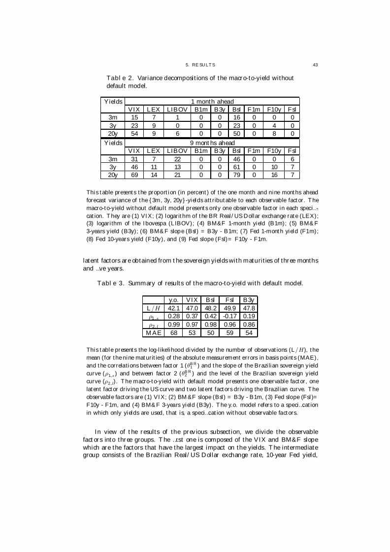
5. RE SULTS 43
Table 2. Variance decompositions of the macro-to-yield withoutdefault model.
Yields 1 month aheadVIX LEX LIBOV B1m B3y Bsl F1m F10y Fsl
3m 15 7 1 0 0 16 0 0 03y 23 9 0 0 0 23 0 4 020y 54 9 6 0 0 50 0 8 0
Yields 9 months aheadVIX LEX LIBOV B1m B3y Bsl F1m F10y Fsl
3m 31 7 22 0 0 46 0 0 63y 46 11 13 0 0 61 0 10 720y 69 14 21 0 0 79 0 16 7
This table presents the proportion (in percent) of the one month and nine months aheadforecast variance of the {3m, 3y, 20y}-yields attributable to each observable factor. Themacro-to-yield without default model presents only one observable factor in each speci…-cation. They are (1) VIX; (2) logarithm of the BR Real/US Dollar exchange rate (LEX);(3) logarithm of the Ibovespa (LIBOV); (4) BM&F 1-month yield (B1m); (5) BM&F3-years yield (B3y); (6) BM&F slope (Bsl) = B3y - B1m; (7) Fed 1-month yield (F1m);(8) Fed 10-years yield (F10y), and (9) Fed slope (Fsl)= F10y - F1m.
latent factors are obtained from the sovereign yields with maturities of three monthsand …ve years.
Table 3. Summary of results of the macro-to-yield with default model.
y.o. VIX Bsl Fsl B3yL/H 42.1 47.0 48.2 49.9 47.8ρ1,s 0.28 0.37 0.42 -0.17 0.19ρ2, l 0.99 0.97 0.98 0.96 0.86
MAE 68 53 50 59 54
This table presents the log-likelihood divided by the number of observations (L/H), themean (for the nine maturities) of the absolute measurement errors in basis points (MAE),and the correlations between factor 1 (θB R
1 ) and the slope of the Brazilian sovereign yieldcurve (ρ1,s) and between factor 2 (θB R
2 ) and the level of the Brazilian sovereign yieldcurve (ρ2,l). The macro-to-yield with default model presents one observable factor, onelatent factor driving the US curve and two latent factors driving the Brazilian curve. Theobservable factors are (1) VIX; (2) BM&F slope (Bsl) = B3y - B1m, (3) Fed slope (Fsl)=F10y - F1m, and (4) BM&F 3-years yield (B3y). The y.o. model refers to a speci…cationin which only yields are used, that is, a speci…cation without observable factors.
In view of the results of the previous subsection, we divide the observablefactors into three groups. The …rst one is composed of the VIX and BM&F slopewhich are the factors that have the largest impact on the yields. The intermediategroup consists of the Brazilian Real/US Dollar exchange rate, 10-year Fed yield,

442 . T HE ROLE O F M AC ROE CONOM IC VARIABLES IN DETE RM INING SOVEREIG N RISK
Fed slope, and IBovespa. The third group presents little e¤ect on yields, beingformed of BM&F 1-month and 3-year yields, and Fed 1-month yield. In order tounderstand the impact of macro variables on the yields in a model with default, weuse both factors of the …rst group, one factor of the second group (Fed slope), andone factor of the third group (BM&F 3-years yield)1 2.
Table 4. Variance decompositions of the yields of the macro-to-yield with default model.
Model y.o. VIX Bsl Fsl B3yFactor Yield 1m 9m 1m 9m 1m 9m 1m 9m 1m 9mθUS 3m 0 1 0 4 0 1 0 6 1 4
3y 0 0 0 2 0 0 0 5 1 220y 0 0 0 1 0 0 0 5 1 2
Macro 3m - - 15 37 1 7 2 14 1 113y - - 25 50 2 8 1 16 0 220y - - 56 70 5 9 1 17 4 3
θB R1 3m 13 26 10 8 25 14 51 23 30 32
3y 1 20 1 2 8 11 24 17 79 8920y 18 12 9 5 7 11 2 13 85 91
θB R2 3m 87 74 75 51 74 77 47 57 68 53
3y 99 80 74 47 89 80 75 63 20 720y 82 88 35 24 88 80 96 65 10 4
This table presents the proportion (in percent) of the one month and nine months aheadforecast variance of the {3m, 3y, 20y}-yields attributable to each observable factor in themacro-to-yield with default model. The macro-to-yield with default model presents oneobservable factor, one latent factor driving the US curve and two latent factors drivingthe Brazilian curve. The observable factors are (1) VIX; (2) BM&F slope (Bsl) = B3y- B1m, (3) Fed slope (Fsl)= F10y - F1m, and (4) BM&F 3-years yield (B3y). They.o. model refers to a speci…cation in which only yields are used, that is, a speci…cationwithout observable factors.
Table 3 summarizes the results of some versions of the macro-to-yield withdefault model. It shows the likelihood, correlations and measurement errors of theyields of each speci…cation. The …rst column refers to the yields only model (y.o.)in which only latent factors are used. The others are macro-to-yield models withVIX, BM&F slope, Fed slope, and BM&F 3-years yield as observable factors. Theinclusion of the U.S. reference curve produces a gain in likelihood and in …t, becausethe measurement errors are lower. The latent factor θ2 remains highly linked tothe level of the sovereign yields.
Table 4 presents the variance decomposition of the {3m, 3y, 20y}-yield for oneand nine months ahead. We see that the VIX is still very important, contributingwith up to 70% of the 20-years yield variation. Other variables accounted for less,but still some e¤ect can be attributed to them. Furthermore, in the y.o. versionthe US factor seems to be insigni…cant.
12Models with other observable factors from the second and third groups were also testedproviding similar qualitative results.

5. RE SULTS 45
Table 5. Variance decompositions of the default probabilities ofthe macro-to-yield with default model.
Model y.o. VIX Bsl Fsl B3yFactor Term 1m 9m 1m 9m 1m 9m 1m 9m 1m 9mθUS 3m 0 0 0 1 0 0 1 4 0 1
3y 0 1 19 60 0 0 4 4 12 2520y 0 1 69 92 5 6 3 3 51 65
Macro 3m - - 54 61 5 9 4 18 8 253y - - 48 26 9 10 20 22 10 2620y - - 19 5 9 9 22 23 9 9
θB R1 3m 22 28 9 7 15 12 34 19 12 21
3y 27 29 6 3 12 11 17 15 11 1820y 27 29 2 1 11 11 15 15 11 24
θB R2 3m 78 72 37 30 80 79 62 60 70 56
3y 73 71 27 11 79 78 60 59 45 3120y 73 71 10 02 74 74 59 59 16 6
This table lists the contribution (in percent) of each factor to the one month and ninemonths ahead forecast of the {3m, 3y, 20y} default probabilities within the macro-to-yieldwith default model.
We also calculate the variance decompositions of the logarithm of the defaultprobabilities, which can be seen in Table 5. All results presented in this paper areobtained using a …xed loss given default ` = 50%. This particular choice is, ofcourse, arbitrary, however there is empirical evidence that the mean of the loss rateis around this value (see, for instance, Moody’s, 2008)13 . The VIX is responsiblefor the greatest e¤ect, especially in the short-term. According to the model, inthe 1- and 9-month horizon, VIX accounts, respectively, for 54% and 61% of the3-month default probability. The BM&F and Fed slopes and BM&F 3-year yieldexplain 5%, 4% and 8% for 1-month ahead, and 9%, 18% and 25% for 9-monthahead, respectively, of the 3-month default probability. On the other hand, the Fedslope has the highest explanatory power for long-term default probability amongthe macro factors.
5.3. Bilateral models. In this subsection we present our main model. It hasone American latent factor, one American macro factor (VIX), one Brazilian macrofactor and two Brazilian latent factors. The Brazilian macro factor has a bilateralinteraction with the Brazilian sovereign factors, that is, the macro factors and thesovereign yield curves fully interact. This means that KBR ,B R
M,θ 6= 0. Once more, theAmerican latent factor is obtained from the yield with maturity of three monthswhile Brazilian latent factors are extracted considering that sovereign yields withmaturities of three months and …ve years are priced without error.
We …x VIX as the American macro factor since it presents the best explanatorypower for the simpler models analyzed in the previous subsections. We test four
13In order to verify the sensitivity of the results to the loss rate, we tested other values(` = 25% and ` = 75%) in the macro-to-yield with default model. From a qualitative point ofview the results were very similar.
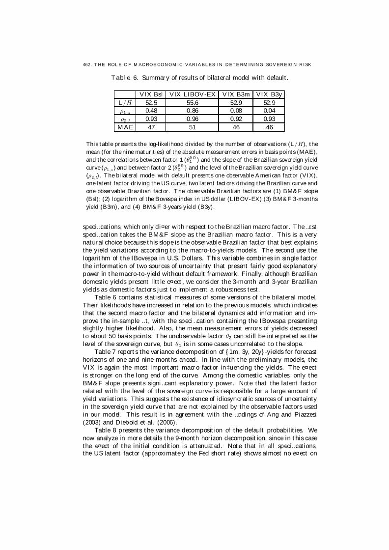
462 . T HE ROLE O F M AC ROE CONOM IC VARIABLES IN DETE RM INING SOVEREIG N RISK
Table 6. Summary of results of bilateral model with default.
VIX Bsl VIX LIBOV-EX VIX B3m VIX B3yL/H 52.5 55.6 52.9 52.9ρ1,s 0.48 0.86 0.08 0.04ρ2, l 0.93 0.96 0.92 0.93
MAE 47 51 46 46
This table presents the log-likelihood divided by the number of observations (L/H), themean (for the nine maturities) of the absolute measurement errors in basis points (MAE),and the correlations between factor 1 (θB R
1 ) and the slope of the Brazilian sovereign yieldcurve (ρ1,s) and between factor 2 (θBR
2 ) and the level of the Brazilian sovereign yield curve(ρ2,l). The bilateral model with default presents one observable American factor (VIX),one latent factor driving the US curve, two latent factors driving the Brazilian curve andone observable Brazilian factor. The observable Brazilian factors are (1) BM&F slope(Bsl); (2) logarithm of the Bovespa index in US dollar (LIBOV-EX) (3) BM&F 3-monthsyield (B3m), and (4) BM&F 3-years yield (B3y).
speci…cations, which only di¤er with respect to the Brazilian macro factor. The …rstspeci…cation takes the BM&F slope as the Brazilian macro factor. This is a verynatural choice because this slope is the observable Brazilian factor that best explainsthe yield variations according to the macro-to-yields models. The second use thelogarithm of the IBovespa in U.S. Dollars. This variable combines in single factorthe information of two sources of uncertainty that present fairly good explanatorypower in the macro-to-yield without default framework. Finally, although Braziliandomestic yields present little e¤ect, we consider the 3-month and 3-year Brazilianyields as domestic factors just to implement a robustness test.
Table 6 contains statistical measures of some versions of the bilateral model.Their likelihoods have increased in relation to the previous models, which indicatesthat the second macro factor and the bilateral dynamics add information and im-prove the in-sample …t, with the speci…cation containing the IBovespa presentingslightly higher likelihood. Also, the mean measurement errors of yields decreasedto about 50 basis points. The unobservable factor θ2 can still be interpreted as thelevel of the sovereign curve, but θ1 is in some cases uncorrelated to the slope.
Table 7 reports the variance decomposition of {1m, 3y, 20y}-yields for forecasthorizons of one and nine months ahead. In line with the preliminary models, theVIX is again the most important macro factor in‡uencing the yields. The e¤ectis stronger on the long end of the curve. Among the domestic variables, only theBM&F slope presents signi…cant explanatory power. Note that the latent factorrelated with the level of the sovereign curve is responsible for a large amount ofyield variations. This suggests the existence of idiosyncratic sources of uncertaintyin the sovereign yield curve that are not explained by the observable factors usedin our model. This result is in agreement with the …ndings of Ang and Piazzesi(2003) and Diebold et al. (2006).
Table 8 presents the variance decomposition of the default probabilities. Wenow analyze in more details the 9-month horizon decomposition, since in this casethe e¤ect of the initial condition is attenuated. Note that in all speci…cations,the US latent factor (approximately the Fed short rate) shows almost no e¤ect on
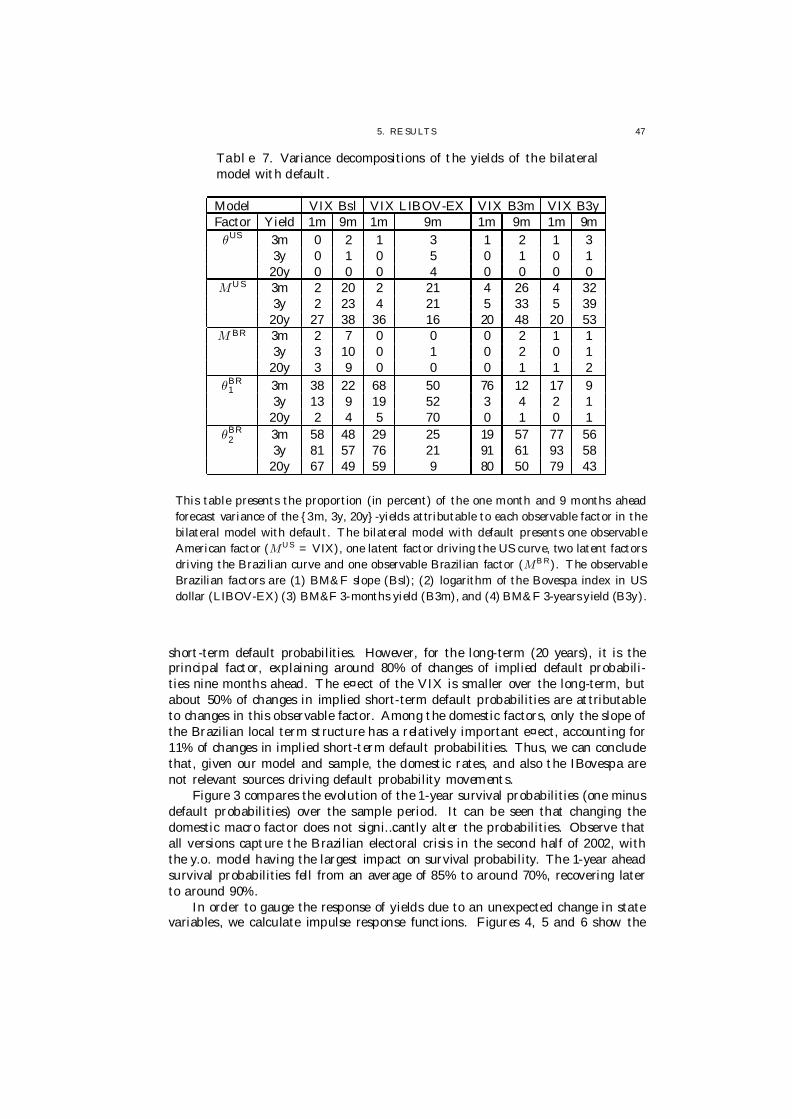
5. RE SULTS 47
Table 7. Variance decompositions of the yields of the bilateralmodel with default.
Model VIX Bsl VIX LIBOV-EX VIX B3m VIX B3yFactor Yield 1m 9m 1m 9m 1m 9m 1m 9mθUS 3m 0 2 1 3 1 2 1 3
3y 0 1 0 5 0 1 0 120y 0 0 0 4 0 0 0 0
MUS 3m 2 20 2 21 4 26 4 323y 2 23 4 21 5 33 5 3920y 27 38 36 16 20 48 20 53
M BR 3m 2 7 0 0 0 2 1 13y 3 10 0 1 0 2 0 120y 3 9 0 0 0 1 1 2
θBR1 3m 38 22 68 50 76 12 17 9
3y 13 9 19 52 3 4 2 120y 2 4 5 70 0 1 0 1
θBR2 3m 58 48 29 25 19 57 77 56
3y 81 57 76 21 91 61 93 5820y 67 49 59 9 80 50 79 43
This table presents the proportion (in percent) of the one month and 9 months aheadforecast variance of the {3m, 3y, 20y}-yields attributable to each observable factor in thebilateral model with default. The bilateral model with default presents one observableAmerican factor (MUS = VIX), one latent factor driving the US curve, two latent factorsdriving the Brazilian curve and one observable Brazilian factor (MB R). The observableBrazilian factors are (1) BM&F slope (Bsl); (2) logarithm of the Bovespa index in USdollar (LIBOV-EX) (3) BM&F 3-months yield (B3m), and (4) BM&F 3-years yield (B3y).
short-term default probabilities. However, for the long-term (20 years), it is theprincipal factor, explaining around 80% of changes of implied default probabili-ties nine months ahead. The e¤ect of the VIX is smaller over the long-term, butabout 50% of changes in implied short-term default probabilities are attributableto changes in this observable factor. Among the domestic factors, only the slope ofthe Brazilian local term structure has a relatively important e¤ect, accounting for11% of changes in implied short-term default probabilities. Thus, we can concludethat, given our model and sample, the domestic rates, and also the IBovespa arenot relevant sources driving default probability movements.
Figure 3 compares the evolution of the 1-year survival probabilities (one minusdefault probabilities) over the sample period. It can be seen that changing thedomestic macro factor does not signi…cantly alter the probabilities. Observe thatall versions capture the Brazilian electoral crisis in the second half of 2002, withthe y.o. model having the largest impact on survival probability. The 1-year aheadsurvival probabilities fell from an average of 85% to around 70%, recovering laterto around 90%.
In order to gauge the response of yields due to an unexpected change in statevariables, we calculate impulse response functions. Figures 4, 5 and 6 show the

482 . T HE ROLE O F M AC ROE CONOM IC VARIABLES IN DETE RM INING SOVEREIG N RISK
Table 8. Variance decompositions of the default probabilities ofbilateral model with default.
Model VIX Bsl VIX LIBOV-EX VIX B3m VIX B3yFactor Term 1m 9m 1m 9m 1m 9m 1m 9mθUS 3m 0 0 2 2 0 0 0 0
3y 7 21 21 59 8 29 9 2920y 47 73 80 93 51 79 52 78
MUS 3m 19 32 16 31 29 42 34 563y 31 31 26 18 36 33 55 5120y 18 11 7 3 20 10 29 16
M BR 3m 8 11 0 0 1 3 1 13y 11 10 1 1 3 3 2 220y 6 3 0 0 1 1 1 1
θBR1 3m 21 12 61 49 11 9 6 3
3y 11 6 38 16 9 7 1 020y 6 2 10 3 5 2 0 0
θBR2 3m 52 44 22 18 59 46 59 39
3y 41 31 14 6 43 29 33 1720y 24 11 3 1 23 8 18 5
This table lists the contribution (in percent) of each factor to the the one month andnine months ahead forecast of the {3m, 3y, 20y} default probabilities within the bilateralmodel with default.
e¤ect of a shock to US latent factor (θUS1 ), VIX and observable domestic factors
(BM&F yields and slope and IBovespa in US Dollars), respectively, on the Brazilian{3m, 3y, 20y}-yields up to 18-months after the shock. The size of the shock is onestandard deviation of a monthly variation of a state variable. In the next threemonths after a shock on VIX, yields rise about 1% and then fall. Changes in eitherthe domestic short or long rate do not result in changes of the sovereign yields. Thesame is true for the domestic stock exchange index (IBovespa). However, a positiveBM&F slope shock causes an increase in the yields. This may indicate a change ofexpectations of a future rise in in‡ation.
We now turn to survival probabilities. Figures 7, 8, 9 show the impact of aone deviation increase of a monthly variation of the US latent factor, VIX andobservable domestic factors, respectively, on the survival probabilities in the nextthree months, three years and twenty years. It shows that the survival probabilityfalls by up to 4% in relative terms due to a shock in the Fed short rate. An increasein VIX also decreases the survival probability about 1.5% in relative terms. Amongthe domestic factors, only the BM&F slope has some impact, decreasing the long-term survival probability by about 0.7% in relative terms.
6. Conclusion
We proposed a model that combines an a¢ne yield dynamics with macro factorsand credit risk. The model was estimated in two steps using the US and Braziliansovereign yield curves. The credit spreads, the macro factors and the US yield curve

6. CO NC LUSION 49
Figure 3. Survival probabilities. This …gure shows the 1-yearsurvival probabilities extracted from some versions of the bilat-eral model and from y.o. model between February 17, 1999 andSeptember 15, 2004. The bilateral model presents one observableAmerican factor (VIX), one latent factor driving the US curve,two latent factors driving the Brazilian curve and one observableBrazilian factor. The observable Brazilian factors are (1) BM&Fslope (Bsl); (2) logarithm of the IBovespa in U.S. dollars (LIBOV-EX) (3) BM&F 3-month yield (B3m), and (4) BM&F 3-year yield(B3y). The y.o. model refers to a speci…cation in which only yieldsare used, that is, a speci…cation without observable factors.
have contemporaneous and lagged interaction. We were able to test how selecteddomestic and external macro factors such as the Brazilian Real/US Dollar exchangerate, VIX (volatility index of S&P 500), IBovespa (São Paulo stock exchange index)and domestic yield curve in‡uence the spreads and default probabilities. The modelwas identi…ed before making restrictions motivated by economic assumptions. Our…ndings indicate that the VIX and U.S. yield curve are the most important factorsdriving the Brazilian sovereign term structure and default probabilities. This resultis consistent with the fact that credit risk premia of sovereign bond are highlycorrelated with the US economic conditions. The VIX has a high impact on 20-year bond yields and on short-term default probabilities, while the fed fund ratehas high explanatory power on the long-term default probabilities. Among thedomestic factors, only the slope of the local yield curve shows a signi…cant e¤ect onthe Brazilian credit spread. However, a signi…cant portion of variations in yields anddefault probabilities are explained by an unobservable factor highly correlated withthe level of the Brazilian sovereign curve. Due to lack of an extensive historicaldataset, we estimated a continuous-time version with daily observations, whichlimited the choices of macro variables. Future work can test monthly models,

502 . T HE ROLE O F M AC ROE CONOM IC VARIABLES IN DETE RM INING SOVEREIG N RISK
Figure 4. Impulse response of shocks to Fed factor on yields.This …gure shows the e¤ect of a shock to Fed factor θUS
1 on theBrazilian sovereign yields with maturities of 3 months, 3 yearsand 20 years up to 18 months after the shock. The shock is onestandard deviation of a monthly variation of the Fed factor. Theresponses are evaluated considering the bilateral model.
Figure 5. Impulse response of shocks to the VIX on yields. This…gure shows the e¤ect of a shock to the VIX on the Brazilian sov-ereign yields with maturities of 3 months, 3 years and 20 years upto 18 months after the shock. The shock is one standard deviationof a monthly variation of the VIX. The responses are evaluatedconsidering the bilateral model.
allowing the use of important variables such as Central Bank reserves, real activityand in‡ation.
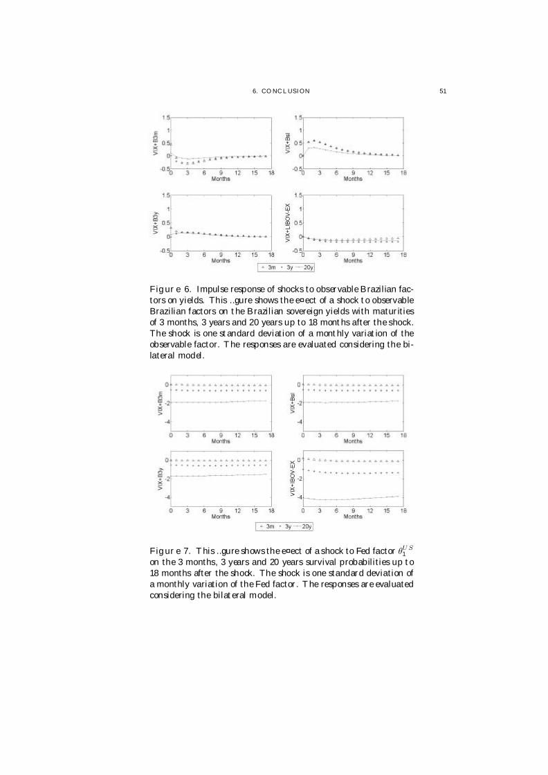
6. CO NC LUSION 51
Figure 6. Impulse response of shocks to observable Brazilian fac-tors on yields. This …gure shows the e¤ect of a shock to observableBrazilian factors on the Brazilian sovereign yields with maturitiesof 3 months, 3 years and 20 years up to 18 months after the shock.The shock is one standard deviation of a monthly variation of theobservable factor. The responses are evaluated considering the bi-lateral model.
Figure 7. This …gure shows the e¤ect of a shock to Fed factor θU S1
on the 3 months, 3 years and 20 years survival probabilities up to18 months after the shock. The shock is one standard deviation ofa monthly variation of the Fed factor. The responses are evaluatedconsidering the bilateral model.

522 . T HE ROLE O F M AC ROE CONOM IC VARIABLES IN DETE RM INING SOVEREIG N RISK
Figure 8. Impulse response of shocks to VIX on survival proba-bilities. This …gure shows the e¤ect of a shock to VIX on the 3months, 3 years and 20 years survival probabilities up to 18 monthsafter the shock. The shock is one standard deviation of a monthlyvariation of the VIX. The responses are evaluated considering thebilateral model.
Figure 9. Impulse response of shocks to observable Brazilian fac-tors on survival probabilities. This …gure shows the e¤ect of ashock to observable Brazilian factors on the 3 months, 3 years and20 years survival probabilities up to 18 months after the shock.The shock is one standard deviation of a monthly variation of theobservable factor. The responses are evaluated considering the bi-lateral model.

CHAPTER 3
Identi…cation of Term Structure Models withObserved Factors
1. Introduction
Multifactor term structure models possess better …tting and forecasting per-formance than single factor models, at the cost of demanding more computationaltime and greater samples for estimation. Hence, it is not surprising that manyauthors restrict the parameter space, sometimes using some economic criteria.
However, restrictions are actually necessary to identify the model: Dai andSingleton (2000), DS, showed that there are transformations of the parametersand state variables of the a¢ne models that preserve the yield curve. Therefore,multiple sub-identi…ed models correspond to the same data.
Arbitrary restrictions, on the other hand, may over-identify some parameters,distorting model properties. Thus, one must …nd a well-de…ned set of restrictionsleading to exact identi…cations. There are 2 approaches in the a¢ne literature, theone by DS and another proposed by Du¢e and Kan (1996) and re…ned by Collin-Dufresne et al. (2006), which uses speci…c transformations of the state factors intoobserved state variables, thereby eliminating unnecessary parameters.
Our contribution relies on the observation that when observed factors are in-cluded in the state vector, new restrictions are needed that take into account theadditional degrees of freedom given by the choice of the relative weight of theobserved factors. Also, we extend the method to other term structure models:the common factor, the Nelson-Siegel, the Legendre and a proposed “quasi” a¢nemodel.
We de…ne invariant operators for each model, and prove that they preserve thelikelihood. Then, we show how to identify.
There are alternative identi…cation choices, which could in principle inducedi¤erent model properties. However, we prove that the yield curve response is thesame for any identi…cation choice. On the other hand, the latent factors responsedoes depend on the choice.
Pericoli and Taboga (2006) also point out to one correctly identi…ed speci…ca-tion of an a¢ne model with observed factors, but they require additional assump-tions.
2. Models
Let Yt = (Y 1t , .., Y n
t )| be the vector of bond yields, Xt = (Mt , θt)| the statevector. Mt 2 Rp and θt 2 Rq denote the observed and latent factors, respectively.
53
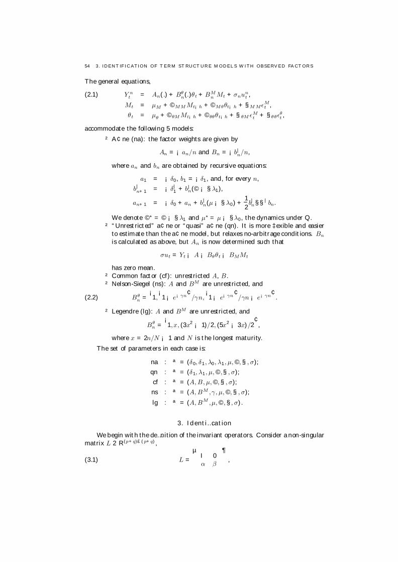
54 3 . IDENT IFIC ATION OF T ERM ST RUCT URE M ODELS W ITH OBSERVED FACT ORS
The general equations,
Y nt = An(.) + Bθ
n(.)θt + BMn Mt + σnun
t ,(2.1)
Mt = µM + ©MM Mt¡h + ©Mθθt¡h + §M MεMt ,
θt = µθ + ©θM Mt¡h + ©θθθt¡h + §θM εMt + §θθεθ
t ,
accommodate the following 5 models:
² A¢ne (na): the factor weights are given by
An = ¡an/n and Bn = ¡b|n/n,
where an and bn are obtained by recursive equations:
a1 = ¡δ0, b1 = ¡δ1, and, for every n,b|
n+1 = ¡δ|1 + b|
n(© ¡ §λ1),
an+1 = ¡δ0 + an + b|n(µ ¡ §λ0) +
12b|n§§| bn.
We denote ©? = © ¡ §λ1 and µ? = µ ¡ §λ0, the dynamics under Q.² “Unrestricted” a¢ne or “quasi” a¢ne (qn). It is more ‡exible and easier
to estimate than the a¢ne model, but relaxes no-arbitrage conditions. Bnis calculated as above, but An is now determined such that
σut = Yt ¡ A ¡ Bθθt ¡ BMMt
has zero mean.² Common factor (cf): unrestricted A, B .² Nelson-Siegel (ns): A and BM are unrestricted, and
(2.2) Bθn =
¡1,
¡1 ¡ e¡γn¢
/γn,¡1 ¡ e¡γn¢
/γn ¡ e¡γn¢.
² Legendre (lg): A and BM are unrestricted, and
Bθn =
¡1,x, (3x2 ¡ 1)/2, (5x2 ¡ 3x)/2
¢,
where x = 2n/N ¡ 1 and N is the longest maturity.
The set of parameters in each case is:
na : ª = (δ0, δ1, λ0, λ1, µ, ©, §, σ);qn : ª = (δ1, λ1, µ, ©,§, σ);cf : ª = (A, B, µ, ©, §, σ);ns : ª = (A, BM ,γ, µ, ©, §, σ);
lg : ª = (A, BM ,µ, ©, §, σ).
3. Identi…cation
We begin with the de…nition of the invariant operators. Consider a non-singularmatrix L 2 R(p+q)£(p+q),
(3.1) L =µ
I 0α β
¶,

3. IDENTIFIC ATION 55
where I 2 Rp£p is the identity, and α 2 Rp£q , β 2 Rq£q . The operator TL acts onfª, Xg:
na : fª, Xg 7! f(δ0, (L| )¡1δ1, λ0, λ1L¡1, Lµ, L©L¡1, L§, σ), LXg;qn : fª, Xg 7! f((L| )¡1δ1, λ1L¡1,Lµ, L©L¡1, L§, σ), LXg;cf : fª, Xg 7! f(A, BL¡1, Lµ, L©L¡1, L§, σ), LXg;ns : fª, Xg 7! f(A, BM ¡ Bθβ¡1α, γ, Lµ, L©L¡1, L§, σ), LXg;
lg : fª, Xg 7! f(A, BM ¡ Bθβ¡1α, Lµ, L©L¡1, L§, σ), LXg.In the ns and lg cases β = I , because Bθ is …xed.
TL transforms the latent factor and adjusts its “macro” content:
(3.2) θt 7! αMt + βθt .
Let ν 2 Rp+q , ν = (0, ν θ)| . The operator Tν shifts the latent factors:
na : fª, Xg 7! f(δ0 ¡ δ|1ν, δ1, λ0 ¡ λ1ν ,λ1, µ + (I ¡ ©)ν , ©, §, σ), X + νg;
qn : fª, Xg 7! f(δ1, λ1, µ + (I ¡ ©)ν , ©, §, σ), X + νg;cf : fª, Xg 7! f(A ¡ Bν, B, µ + (I ¡ ©)ν , ©, §, σ), X + νg;ns : fª, Xg 7! f(A ¡ Bν, BM , γ,µ + (I ¡ ©)ν, ©, §, σ), X + νg;lg : fª, Xg 7! f(A ¡ Bν, BM , µ + (I ¡ ©)ν , ©, §, σ), X + νg.
The last operator, TO , where O 2 Rd£d is a rotation matrix, rotates the pa-rameters related to the Brownian motion and preserves X :
(3.3) § 7! §O| .
TO is related to the VAR ordering of the state variables with respect to endogeneity.The operators are constructed so as to preserve the short rate, the risk premium
and the observed factors. In fact, they preserve the likelihood, as is shown next.The format of the likelihood depends on the type of treatment for the stochasticsingularity that appears when there are more maturities than latent factors. Thecase with Chen-Scott inversion was discussed in chapter 2.
Proposition 2. Given initial conditions em0 = Lm0 and eC0 = LC0L|, theinvariant transformations preserve the likelihood with the Kalman Filter.
Proof. We show that the marginal and full-information likelihoods are pre-served, i.e.,
L(Y jM, ª) = L(Y jM, eª) and L(Y jX, ª) = L(Y j eX, eª),
where ( eX, eª) are the transformed variables and parameters. This is easily seen forthe full information likelihood, which is given by
(3.4) L(Y jX, ª) =Y
tf (Ytjθt, Mt , ª)
(3.5) =Y
texp
©¡1/2£ln jσσ |j + (Yt ¡ A ¡ BXt)| (σσ| )¡1 (Yt ¡ A ¡ BXt)
¤ª.
We turn to the marginal likelihood case, given by
L(Y jM, ª) =Y
tf (YtjYt¡1, Mt¡1, ª)
(3.6) =Y
texp
©¡1/2
£jQt j + (Yt ¡ ft)| Q¡1
t (Yt ¡ ft)¤ª
,
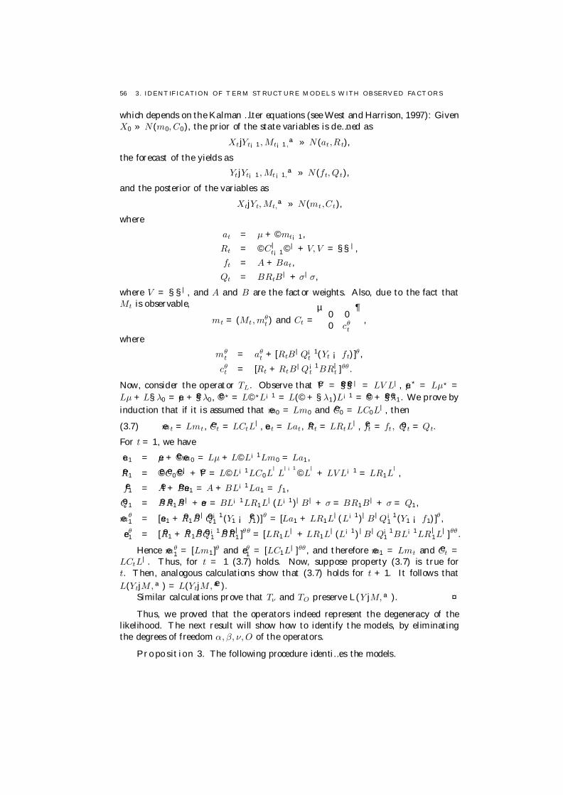
56 3 . IDENT IFIC ATION OF T ERM ST RUCT URE M ODELS W ITH OBSERVED FACT ORS
which depends on the Kalman …lter equations (see West and Harrison, 1997): GivenX0 » N (m0, C0), the prior of the state variables is de…ned as
Xt jYt¡1, Mt¡1,ª » N (at ,Rt),
the forecast of the yields as
Yt jYt¡1, Mt¡1,ª » N (ft, Qt),
and the posterior of the variables as
XtjYt, Mt,ª » N (mt ,Ct),
where
at = µ + ©mt¡1,Rt = ©C|
t¡1©| + V, V = §§|,
ft = A + Bat ,Qt = BRtB| + σ| σ,
where V = §§| , and A and B are the factor weights. Also, due to the fact thatMt is observable,
mt = (Mt , mθt ) and Ct =
µ0 00 cθ
t
¶,
where
mθt = aθ
t + [RtB| Q¡1t (Yt ¡ ft)]θ ,
cθt = [Rt + RtB|Q¡1
t BR|t ]θθ .
Now, consider the operator TL. Observe that eV = e§e§| = LV L| , eµ? = Lµ? =Lµ + L§λ0 = eµ + e§λ0, e©? = L©?L¡1 = L(© + §λ1)L¡1 = e© + e§eλ1. We prove byinduction that if it is assumed that em0 = Lm0 and eC0 = LC0L| , then
(3.7) emt = Lmt , eCt = LCtL| , eat = Lat , eRt = LRtL| , eft = ft , eQt = Qt.
For t = 1, we have
ea1 = eµ + e©em0 = Lµ + L©L¡1Lm0 = La1,eR1 = e© eC0e©| + eV = L©L¡1LC0L
|L
|¡1©L
|+ LV L¡1 = LR1L
|,
ef1 = eA + eBea1 = A + BL¡1La1 = f1,eQ1 = eB eR1 eB| + eσ = BL¡1LR1L| (L¡1)| B| + σ = BR1B| + σ = Q1,
emθ1 = [ea1 + eR1
eB| eQ¡11 (Y1 ¡ ef1)]θ = [La1 + LR1L|(L¡1)| B|Q¡1
1 (Y1 ¡ f1)]θ ,
ecθ1 = [ eR1 + eR1
eB eQ¡11
eB eR|1 ]θθ = [LR1L| + LR1L| (L¡1)|B| Q¡1
1 BL¡1LR|1L
| ]θθ .
Hence emθ1 = [Lm1]θ and ecθ
1 = [LC1L| ]θθ , and therefore em1 = Lmt and eCt =LCtL| . Thus, for t = 1 (3.7) holds. Now, suppose property (3.7) is true fort. Then, analogous calculations show that (3.7) holds for t + 1. It follows thatL(YtjM, ª) = L(YtjM, eª).
Similar calculations prove that Tν and TO preserve L(Y jM, ª). ¤
Thus, we proved that the operators indeed represent the degeneracy of thelikelihood. The next result will show how to identify the models, by eliminatingthe degrees of freedom α, β, ν, O of the operators.
Proposition 3. The following procedure identi…es the models.

3. IDENTIFIC ATION 57
Proof. i) For all models, the operator Tν can be used to set µθ = 0, and theoperator TO to impose a lower triangular form for §.
ii) However, the use of TL will depend on the type of model. Consider the nacase. The identi…cation is achieved by spending the restrictions on any parameter,but mainly on §, ©, ©? or λ1.
iii) Restriction on §: α and β are chosen such that e§θM = 0 and e§θθ = I, i.e.,
L§ =µ
I 0α β
¶ µ§MM 0§θM §θθ
¶=
µ§MM 0
0 I
¶,
where e§ = L§. This does not exhausts the free parameters. So, we apply the trans-formation TS := TLjα = 0, β = S rotation matrix, such that ©θθ or ©?
θθ becomeslower triangular. The operator TS commutes with L§ so that it will only rotateorthogonal Brownian motions, preserving other parameters. This completes theidenti…cation. Another option is obtained by choosing β such that §θθ is diagonaland then apply TD := TLjα = 0,β = D diagonal matrix, such that δθ = 1:
(D¡1)|δ =µ
I 00 D¡1
¶ µδMδθ
¶=
µδM1
¶.
iv) Restriction on λ1:
λ1L¡1 =µ
λMM1 λMθ
1λθM
1 λθθ1
¶ µI 0
¡β¡1α β¡1
¶=
ÃeλMM
1eλMθ
10 I
!,
so that we eliminate λθM1 and λθθ
1 . Similarly, we could restrict λ0 instead of µ.v) Restriction on © or ©?. This case is harder, because it involves quadratic
equations. To avoid this, we assume that © can be decomposed as P¤P ¡1, where¤ is a real diagonal matrix. If © has real and distinct eigenvalues, this is alwayspossible. Since © = P ¤P¡1, then L©L¡1 = LP ¤(LP )¡1. Now, α can be chosensuch that LP becomes upper block triangular (ubt), that is,
LP =µ
I 0α β
¶ µPMM PMθPθM Pθθ
¶=
µPM M PMθ
0 Pθθ
¶.
Then (LP )¡1 and the transformed e© = L©L¡1 will also be ubt. That is, e©θM = 0.The …rst identi…cation of this type is the following. Choose β such that βPθθ is adiagonal matrix, then e©θθ will also be diagonal. Next, use TD such that δθ = 1,completing the identi…cation. Alternatively, we could have started with ©? =P¤?P¡1. Yet another possibility is to impose a lower triangular βPθθ , which impliesin a lower triangular e©θθ . Then use TT := TLjα = 0, β = T lower triangular matrixto impose a diagonal §θθ . Finally, the identi…cation …nishes by applying TD suchthat δθ = 1.
vi) For the other models, the procedure is entirely analogous, except that inthe case of lg and ns models, there are less degrees of freedom, for β = I . ¤
Table 1 shows a summary of identi…cations for the a¢ne model. Type 2 assumethat © or ©? can be decomposed as P¤P¡1. Otherwise, we call Type 1.
Table 1. Summary of identi…cations (a¢ne case).

58 3 . IDENT IFIC ATION OF T ERM ST RUCT URE M ODELS W ITH OBSERVED FACT ORS
©θM ©θθ ©?θM ©?
θθ §θM §θθ δθ λ1θM λ1
θθType1 Full Full Full L Tr 0 I Full - -Type1 Full Full Full L Tr 0 Diag I - -Type1 Full L Tr Full Full 0 I Full - -Type1 Full L Tr Full Full 0 Diag I - -Type1 Full Full - - Full L Tr Full 0 IType1 - - Full Full Full L Tr Full 0 IType2 Full Full 0 Diag Full L Tr I - -Type2 Full Full 0 L Tr Full Diag I - -Type2 0 Diag Full Full Full L Tr I - -Type2 0 L Tr Full Full Full Diag I - -
Since there are many options, it is not clear how to choose a speci…cation.At least, our next proposition shows that the response of the yield and observedvariables to state factor shocks (IRFY, IRFM) and the variance decomposition ofthe yield (VDY) is the same for any case. In practice, however, at the inferencestage, some alternatives may prove easier to be estimated.
Proposition 4. TL and Tν preserve IRFY, VDY and IRFM. All operatorspreserve the yield curve.
Proof. First note that for the qn, cf, ns and lg models, the invariance of theyields is immediate. Consider the na model. The weights A, Bjfª, Xg change toA, BL¡1jTLfª, Xg when TL is applied, for b|
n+1L¡1 = ¡δ|
1L¡1 + b|
nL¡1(L©L¡1 ¡L§λ1L¡1) and an+1 = ¡δ0 + an + b|
nL¡1(Lµ¡L§λ0)+ 12 b|
nL¡1L§§|L| (L¡1)|bn.It follows that Yt = A + BL¡1LXt + σut, which proves the invariance under TL.
Furthermore, similar computations show that A, Bjfª, Xg changes to A ¡Bν, B jTν fª, Xg. Thus, an+1jfª, Xg becomes an+1 ¡ b|
n+1νjTν fª, Xg, so thatYt = A ¡ Bν + B(Xt + ν ) + σut , which proves the invariance under Tν.
Now, IRFY, VDYj and IRFM, given by fB©n§εtgn, fB§j (B§j )| + ... +B©n§j (B©n§j )|gn and the …rst p lines of LB©n§εt , are all easily seen to bepreserved under TL and Tν . ¤
On the other hand, the response of the latent factors to factor shocks, IRFθ,depends on the identi…cation: L©n§εt . This has implications on the interpreta-tion of the latent factors, specially regarding monetary policy rules, since di¤erentspeci…cations will give di¤erent “weights” to the macro content of the latent factors.
4. Conclusion
We specify invariant operators and prove that they preserve the likelihood ofterm structure models with observed factors. Hence, restriction choices must bemade in order to identify the model, and we show ways of achieving it.
It turns out that any speci…cation, if correctly estimated, lead to the sameobservable model properties such as the response of the yield curve to state variableshocks. However, some speci…cations can be numerically simpler to estimate. Also,the interpretation of the latent factors varies with the speci…cation.

CHAPTER 4
Forecasting the Yield Curve: Comparing Models
1. Introduction
The modeling of the term structure of interest rates is a challenging task thathas, from a practical perspective, at least three purposes. Firstly, with this toolavailable, one can price …xed income instruments and manage risk of bonds andderivatives. Secondly, it allows monitoring of observed and unobserved economicvariables such as risk premium, default risk, in‡ation and real activity. Finally, itis possible to forecast futures interest rates.
In this study, we address the latter issue using a rich class of linear factor mod-els. Examples of users of yield curve forecasts are numerous. Treasuries manage theemission and maintenance of the stock of public debt, which continuously demandsan assessment of current and future interest rates. Investors must track their port-folios performance against the cost of opportunity of investing in low risk bonds.Central Banks react to the expected in‡ation and economic activity adjusting theshort rate, thereby a a¤ecting the whole curve.
Term structure models can be classi…ed in di¤erent ways. If restrictions to theevolution of the yields are imposed in order to avoid risk-free pro…t opportunities,then the model is known as arbitrage-free. Otherwise the model is said to be purelystatistical. Arbitrage-free models contain some ingredients arising from equilibriummodels having thus a strong economic appeal. Seminal works within this class areVasicek (1977), Cox et al. (1985) and Heath et al. (1992) while Nelson and Siegel(1987) and Svensson (1994) are pioneer works in the class of statistical models.Moreover, term structure models may directly include or not macroeconomic and…nancial factors driving the yield curve. Among others, we can cite the works of Angand Piazzesi (2003), Diebold et al. (2005), Hördahl et al. (2006), and Ludvigsonand Ng (2007) that use macroeconomic variables to model the term structure ofinterest rate. Finally, the relation between factors and interest rates may be linearor assume a more general speci…cation. Examples of linear models are the classof a¢ne models studied by Du¢e and Kan (1996)1, while Longsta¤ (1989) andLeippold and Wu (2003) constitute examples of non-linear models.
Although several works from macroeconomics, …nance and econometrics havebeen devoted to term structure models, few of them analyzed the out-of-sample fore-casting performance. Predictability questions regarding yield curve are …rst studiedby Fama and Bliss (1987) who investigated the relationship between forward andfuture spot rates. More recently, Du¤ee (2002) documents that the a¢ne modelsproduced poor U.S. yields forecasts. Diebold and Li (2006) propose a two-stagemodel based on the Nelson and Siegel (1987) framework to forecast the U.S. term
1An a¢ne model is an arbitrage-free term structure model, such that the state process X isan a¢ne di¤usion, and the yields are also a¢ne in X.
59
60 4. FOREC AST ING THE YIE LD CURVE: C OM PARING M ODELS
structure that presented better results than some competing models. Nevertheless,Almeida and Vicente (2008) show that the inclusion of no-arbitrage conditions ina latent model improves the out-of-sample …t. Ang and Piazzesi (2003) …nd thatan a¢ne model with macroeconomic variables outperforms the unrestricted VARmodel containing the same observable factors. They also show that models withmacro factors forecast better than models with only unobservable factors. In thesame line, Hördahl et al. (2006) con…rm that the forecasting performance of amodel with observable factors is superior to models based on latent factors.
The papers cited in the last paragraph deal with models where the interest ratesare linear functions of state factors (observable or latent). Due to variety of reasons(the more important is the ease of implementation), linear models are nowadays theworkhorse of yield curve modeling. However, to the best of our knowledge there isno study based on the same dataset that provides a full comparison of the in-sampleand out-of-sample performance of di¤erent speci…cations of linear models. In thisarticle we try to …ll this gap in the …nance literature. Although some recent studieshave addressed the forecasting performance of di¤erent linear interest rate models2,we believe that no one has implemented a comparative analysis as comprehensiveas ours. We analyze arbitrage-free and purely statistical models, with or withoutobservable variables. In addition to testing the models with U.S. data as usual, wealso consider a database from a emerging country. For instance, Laurini and Hotta(2007), Pinheiro et al. (2007), Almeida et al. (2007A, 2007B) and Shoucha (2005)present models estimated for Brazilian data.
All the models analyzed in this study present constant volatility. Although sto-chastic volatility processes have some desirable properties, the standard approachin the interest rates forecasting has been using homocedastic models. Besides theparsimonious, constant volatility models seems to be a natural choice when the aimis forecasting since in this family there is no factor collecting information about thevolatility process. Therefore, it is expected that the mean of the yields distributioncan be better captured.
We estimated the models via MCMC (see chapter 1), which will allow themeasurement of the uncertainty associated to the information available for theestimation of a given model.
2. Models
As before, Y denote the vector of n interest rate yields, X = (M, θ) the statevector composed of p macro factors and q latent factors. As explained in theprevious chapter, the general equations for the latent factor models are:
(2.1) Yt = A(.) + Bθ(.)θt + BMMt + σut , ut » N (0, In),
(2.2) Xt = µ + ©Xt¡h + §εt , εt » N (0, Ip+q),
where h denotes the lag size, and A(.) and B(.) di¤erentiate the models.For the Fama-Bliss case, the data is monthly and h = 1. The other samples
are daily and h = 1, 5 or 21. This last choice turns a daily model into a sum ofmonthly models: since there are on average 21 business days in a month, whenh = 21, the sample can be decomposed into 21 disjoint series and the full data
2Besides the works cited above, we can also include Vicente and Tabak (2008) and Moench(2008).
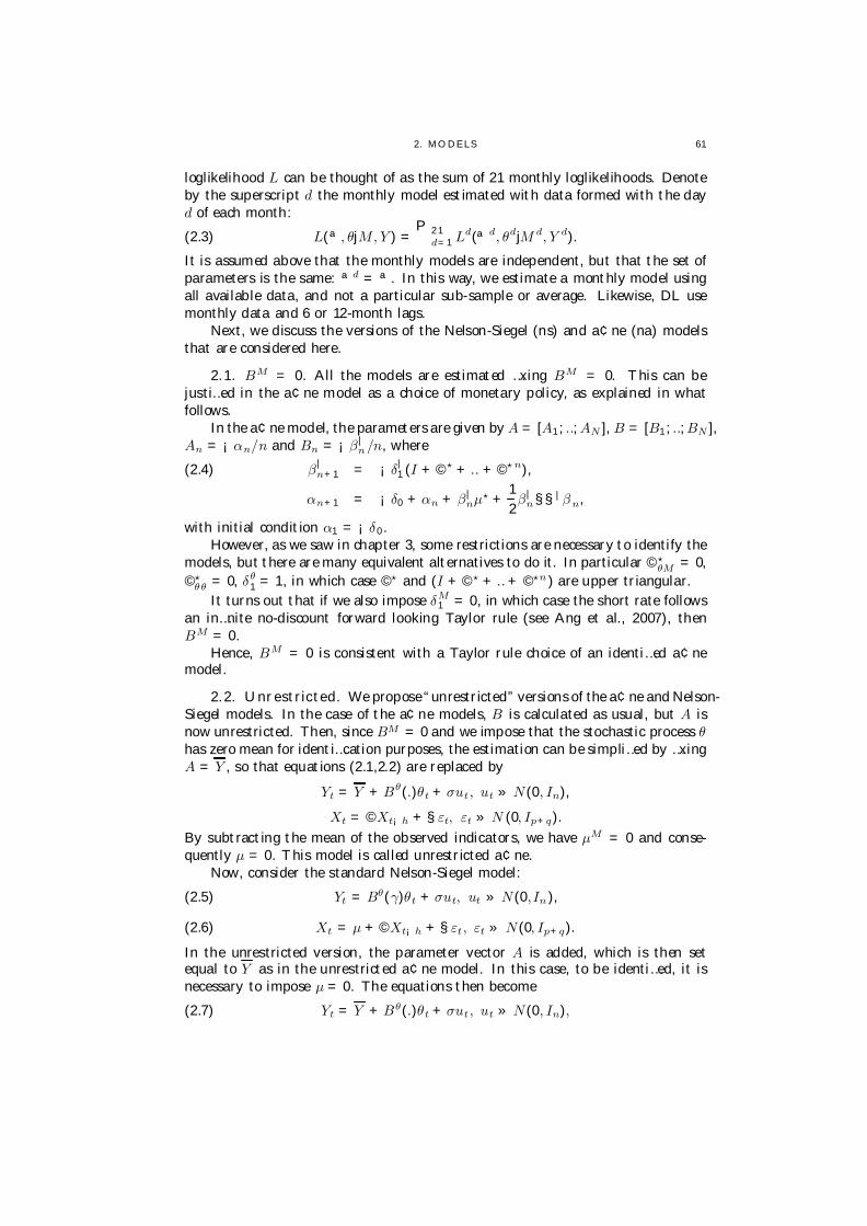
2. MO DELS 61
loglikelihood L can be thought of as the sum of 21 monthly loglikelihoods. Denoteby the superscript d the monthly model estimated with data formed with the dayd of each month:
(2.3) L(ª, θjM, Y ) =P21
d=1 Ld(ªd, θdjM d, Y d).
It is assumed above that the monthly models are independent, but that the set ofparameters is the same: ªd = ª. In this way, we estimate a monthly model usingall available data, and not a particular sub-sample or average. Likewise, DL usemonthly data and 6 or 12-month lags.
Next, we discuss the versions of the Nelson-Siegel (ns) and a¢ne (na) modelsthat are considered here.
2.1. BM = 0. All the models are estimated …xing BM = 0. This can bejusti…ed in the a¢ne model as a choice of monetary policy, as explained in whatfollows.
In the a¢ne model, the parameters are given by A = [A1; ..; AN ], B = [B1; ..; BN ],An = ¡αn/n and Bn = ¡β|
n/n, where
β|n+1 = ¡δ|
1 (I + ©? + .. + ©? n),(2.4)
αn+1 = ¡δ0 + αn + β|nµ? +
12β|
n§§|βn,
with initial condition α1 = ¡δ0.However, as we saw in chapter 3, some restrictions are necessary to identify the
models, but there are many equivalent alternatives to do it. In particular ©?θM = 0,
©?θθ = 0, δθ
1 = 1, in which case ©? and (I + ©? + .. + ©?n ) are upper triangular.It turns out that if we also impose δM
1 = 0, in which case the short rate followsan in…nite no-discount forward looking Taylor rule (see Ang et al., 2007), thenBM = 0.
Hence, BM = 0 is consistent with a Taylor rule choice of an identi…ed a¢nemodel.
2.2. Unrestricted. We propose “unrestricted” versions of the a¢ne and Nelson-Siegel models. In the case of the a¢ne models, B is calculated as usual, but A isnow unrestricted. Then, since BM = 0 and we impose that the stochastic process θhas zero mean for identi…cation purposes, the estimation can be simpli…ed by …xingA = Y , so that equations (2.1,2.2) are replaced by
Yt = Y + Bθ(.)θt + σut , ut » N (0, In),
Xt = ©Xt¡h + §εt, εt » N (0, Ip+q).By subtracting the mean of the observed indicators, we have µM = 0 and conse-quently µ = 0. This model is called unrestricted a¢ne.
Now, consider the standard Nelson-Siegel model:
(2.5) Yt = Bθ(γ)θt + σut, ut » N (0,In ),
(2.6) Xt = µ + ©Xt¡h + §εt , εt » N (0, Ip+q).
In the unrestricted version, the parameter vector A is added, which is then setequal to Y as in the unrestricted a¢ne model. In this case, to be identi…ed, it isnecessary to impose µ = 0. The equations then become
(2.7) Yt = Y + Bθ(.)θt + σut , ut » N (0, In),
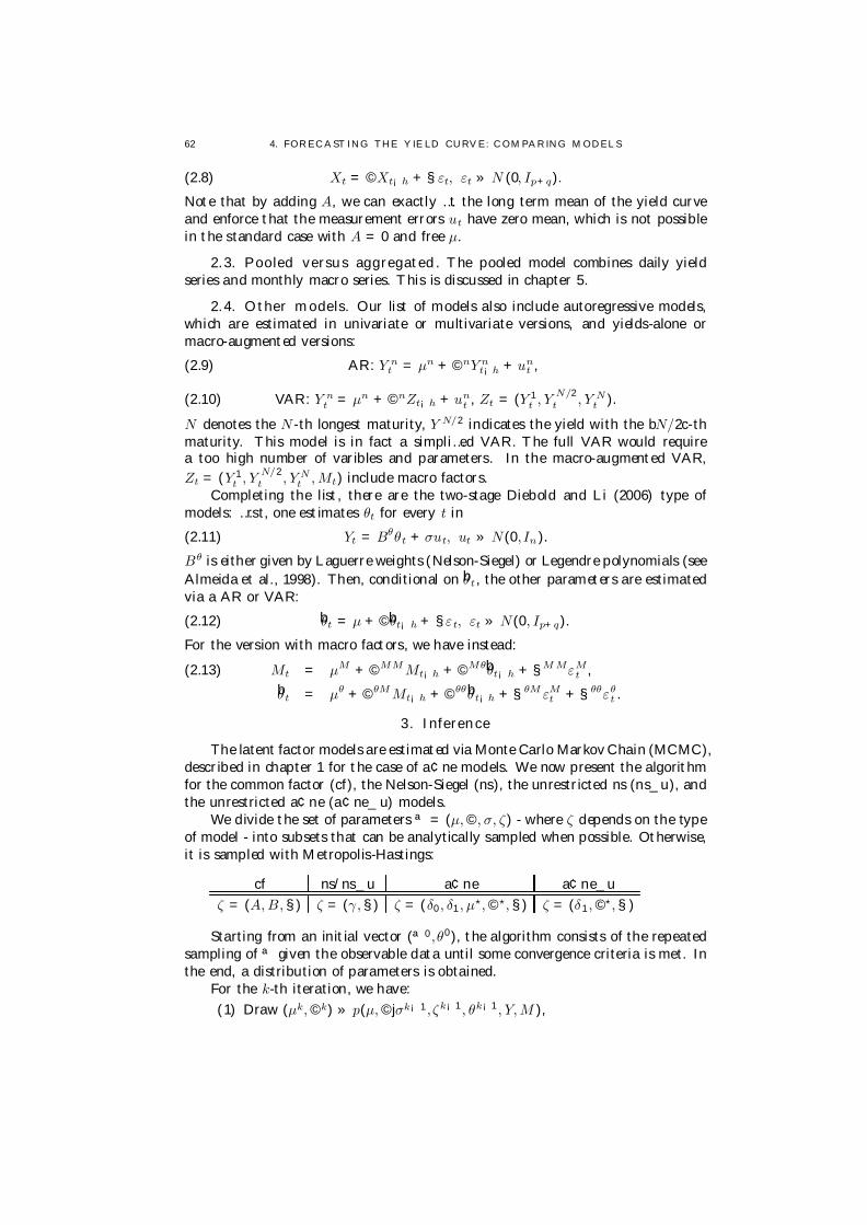
62 4. FOREC AST ING THE YIE LD CURVE: C OM PARING M ODELS
(2.8) Xt = ©Xt¡h + §εt, εt » N (0, Ip+q).
Note that by adding A, we can exactly …t the long term mean of the yield curveand enforce that the measurement errors ut have zero mean, which is not possiblein the standard case with A = 0 and free µ.
2.3. Pooled versus aggregated. The pooled model combines daily yieldseries and monthly macro series. This is discussed in chapter 5.
2.4. Other models. Our list of models also include autoregressive models,which are estimated in univariate or multivariate versions, and yields-alone ormacro-augmented versions:
(2.9) AR: Y nt = µn + ©nY n
t¡h + unt ,
(2.10) VAR: Y nt = µn + ©nZt¡h + un
t , Zt = (Y 1t , Y N/2
t , Y Nt ).
N denotes the N -th longest maturity, Y N/2 indicates the yield with the bN/2c-thmaturity. This model is in fact a simpli…ed VAR. The full VAR would requirea too high number of varibles and parameters. In the macro-augmented VAR,Zt = (Y 1
t , Y N/2t , Y N
t , Mt) include macro factors.Completing the list, there are the two-stage Diebold and Li (2006) type of
models: …rst, one estimates θt for every t in
(2.11) Yt = Bθθt + σut, ut » N (0,In ).
Bθ is either given by Laguerre weights (Nelson-Siegel) or Legendre polynomials (seeAlmeida et al., 1998). Then, conditional on bθt , the other parameters are estimatedvia a AR or VAR:
(2.12) bθt = µ + ©bθt¡h + §εt, εt » N (0, Ip+q).
For the version with macro factors, we have instead:
Mt = µM + ©MM Mt¡h + ©Mθbθt¡h + §M MεMt ,(2.13)
bθt = µθ + ©θM Mt¡h + ©θθbθt¡h + §θM εMt + §θθεθ
t .
3. Inference
The latent factor models are estimated via Monte Carlo MarkovChain (MCMC),described in chapter 1 for the case of a¢ne models. We now present the algorithmfor the common factor (cf), the Nelson-Siegel (ns), the unrestricted ns (ns_u), andthe unrestricted a¢ne (a¢ne_u) models.
We divide the set of parameters ª = (µ, ©, σ, ζ) - where ζ depends on the typeof model - into subsets that can be analytically sampled when possible. Otherwise,it is sampled with Metropolis-Hastings:
cf ns/ns_u a¢ne a¢ne_uζ = (A, B, §) ζ = (γ, §) ζ = (δ0, δ1, µ?, ©?, §) ζ = (δ1, ©?, §)
Starting from an initial vector (ª0,θ0), the algorithm consists of the repeatedsampling of ª given the observable data until some convergence criteria is met. Inthe end, a distribution of parameters is obtained.
For the k-th iteration, we have:(1) Draw (µk, ©k) » p(µ, ©jσk¡1,ζk¡1, θk¡1, Y, M ),

3. INFERENC E 63
(2) Draw σk » p(σjµk, ©k, ζk¡1, θk¡1, Y, M),(3) Draw θk » p(θjµk, ©k, σk , ζk¡1, Y, M),(4) Draw ζk
i » p(ζi jµk , ©k, σk ,θk , ζk¡1¡i , Y , M).
Thus, the estimation problem is decomposed into a series of simpler sub-problems. Sub-problems 1-3 use Gibbs sampling, and correspond to, respectively,the estimation of a VAR model, the estimation of its variance, and the joint distri-bution of latent factors:
Subproblem 1:
(3.1) f (µ, ©jσk¡1, ζk¡1,θk¡1, Y ,M ) » N ((X| X)¡1X| X?, (X| X)¡1 §),
where X = (X1, ..., XT¡1)|, X ? = (X2, ..., XT )| , X = (M, θ).Subproblem 2:
(3.2) f (σjµk, ©k, ζk¡1, θk¡1, Y, M) » IG(diag(U| U),n),
where U = Y ¡ A ¡ BX, and IG is the inverse gamma distribution.Subproblem 3:
(3.3) f (θjµk ,©k ,σk, ζk¡1, Y, M ).
This problem is solved via the FFBS algorithm (Carter and Kohn, 1994), seen inchapter 1.
The step relative to ζ is model speci…c:Subproblem 4:
(3.4) f (ζ ijζk¡1¡i , µk, ©k, σk , θk , Y, M).
² §: For the ns, a¢ne_u and cf cases, there is a known distribution, givenby the inverse wishart distribution. For the a¢ne case, we sample us-ing Independence Metropolis with an inverse wishart proposal: draw acandidate ζk
i » ζk¡1i + N (0, c), where c is a constant. If
(3.5) L(ζki jζk¡1
¡i , µk, ©k, σk , θk , Y, M ) ¡ L(ζki jζk¡1
¡i , µk , ©k , σk, θk, Y ,M ) > log(z),
where L is the log-likelihood and z » U(0, 1), then accept it, otherwiseζk
i = ζk¡1i . By calibrating c, the acceptance ratio is maintained in the
20-50% range.² δ0, µ?: a¢ne case. Usually, these parameters are estimated via Metropolis.
However, as noticed by Johannes and Polson (2006), µ? appears in alinear way on the pricing equation. Based on this, we analytically derivea distribution for µ?. Rearranging the recursive equations, one obtains:
Bn = δ|1 (I + ©? + .. + ©?n¡1)/n,(3.6)
An = δ0 + ηnµ? + ζn,ηn = (B1 + .. + Bn),ζn = ¡n(B1§§| B|
1 + .. + Bn¡1§§| B|n¡1).
Hence
Y nt = An + BnXt + σnun
t(3.7)= δ0 + ηnµ? + ζn + BnXt + σnun
t ,eY n
t : = Y nt ¡ BnXt ¡ ζn = δ0 + ηnµ? + σnun
t ,
so that δ0,µ? can be solved by generalized least squares.² δ1, ©?: a¢ne case. Use random walk Metropolis with normal proposal.

64 4. FOREC AST ING THE YIE LD CURVE: C OM PARING M ODELS
² γ : ns case. Use random walk Metropolis with normal proposal.² A: cf, a¢ne_u and ns_u cases. Set A = Y .² B : cf case. The solution is a regression similar to that for µ, ©.
3.1. Performance Criteria and speci…cations.3.1.1. In-sample Information Criterion. Due to the fact that the models under
investigation have a di¤erent number of parameters, it is not possible to compareabsolute values of the likelihood. Therefore, we choose as our criteria two Bayesianmeasures that emphasize forecasting performance and adherence to data, takinginto account the number of parameters. Gelfand and Ghosh (1998) proposed theminimum posterior predictive loss (PPL) criterion emphasizing forecasting per-formance and Spiegelhalter (2002) proposed the deviance of information criterion(DIC) emphasizing adherence.
² PPL: For each realization of the distribution of the parameter estimatorsªw » (ªjY ), there corresponds a yield curve forecast Y j ªw. Considera loss function penalizing both the expected error E(Y jªw) ¡ Y and thevariance of the forecasts Y jªw ¡E(Y jªw ). In our case, the target variableis multivariate, so that we take the mean of the expected losses calculatedfor each maturity. In other words, the criterion is:
(3.8)
PPL =X
n
X
t
(Y nt ¡ E(Y n
t jDt¡h))2+12
X
n
X
t
1Nw
X
w
(E(Y nt jªw ) ¡ E(Y n
t jDt¡h))2 ,
where Nw is the number of realizations.² DIC: It consists of a generalization of the Akaike criterion (AIC), based
on the distribution of the divergence D(ª) = ¡2logL(ª):
(3.9) DIC = Ew (D(ªw )) ¡ pd = 2E(D(ª)) ¡ D(Ew (ªw )),
where pd = E(D(ª)) ¡ D(E(ª)) measures the equivalent number of pa-rameters in the model, E(D(ª)) is the mean of the divergences calculatedwith the estimators’ posterior distribution, and D(E(ª)) is the divergencecalculated at the mean point of the estimators’ posterior distribution.
The choice of the criterion should be linked to the objective of the estimation.Banerjee et al. (2004) show that PPL and DIC evaluates the goodness of …tting ofthe models penalizing for the degree of complexity. DIC considers the likelihood onthe space of the parameters and PPL on the posterior predictive space. Thus, whenthe main interest lies in forecasting, PPL is preferred, whereas when the capacityof the model to explain the data is more desirable, DIC should be used.
Besides those measures, we will calculate models in-sample RMSE normalizedby the random walk (RW) RMSE.
3.1.2. Out-of-sample Criterion. To compare the out-of-sample results, we de-…ne 3 measures using the Theil-U, the ratio between the RMSE of the model fore-casts and the RMSE of the RW forecasts. When the processes under study havehigh persistency, RW frequently adheres well to data, sometimes even more thansophisticated models.
TU(n) =
ÃX
tout
(Y nt ¡ bY n
tjt¡h)2/X
tout
(Y nt ¡ Y n
t¡h)2! 1
2
.
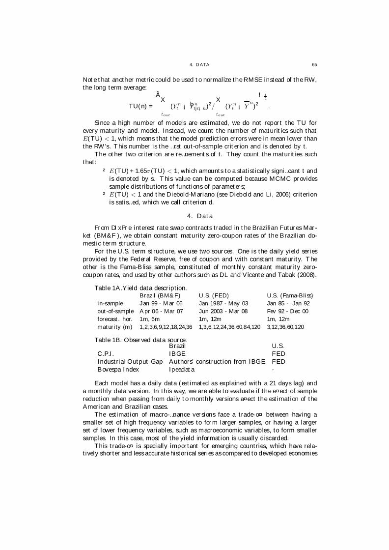
4. DATA 65
Note that another metric could be used to normalize the RMSE instead of the RW,the long term average:
TU(n) =
ÃX
tout
(Y nt ¡ bY n
tjt¡h)2/X
tout
(Y nt ¡ Y
n)2
! 12
.
Since a high number of models are estimated, we do not report the TU forevery maturity and model. Instead, we count the number of maturities such thatE(TU) < 1, which means that the model prediction errors were in mean lower thanthe RW’s. This number is the …rst out-of-sample criterion and is denoted by t.
The other two criterion are re…nements of t. They count the maturities suchthat:
² E(TU)+1.65σ (TU) < 1, which amounts to a statistically signi…cant t andis denoted by s. This value can be computed because MCMC providessample distributions of functions of parameters;
² E(TU) < 1 and the Diebold-Mariano (see Diebold and Li, 2006) criterionis satis…ed, which we call criterion d.
4. Data
From DIxPre interest rate swap contracts traded in the Brazilian Futures Mar-ket (BM&F ), we obtain constant maturity zero-coupon rates of the Brazilian do-mestic term structure.
For the U.S. term structure, we use two sources. One is the daily yield seriesprovided by the Federal Reserve, free of coupon and with constant maturity. Theother is the Fama-Bliss sample, constituted of monthly constant maturity zero-coupon rates, and used by other authors such as DL and Vicente and Tabak (2008).
Table 1A.Yield data description.Brazil (BM&F) U.S. (FED) U.S. (Fama-Bliss)
in-sample Jan 99 - Mar 06 Jan 1987 - May 03 Jan 85 - Jan 92out-of-sample Apr 06 - Mar 07 Jun 2003 - Mar 08 Fev 92 - Dec 00forecast. hor. 1m, 6m 1m, 12m 1m, 12mmaturity (m) 1,2,3,6,9,12,18,24,36 1,3,6,12,24,36,60,84,120 3,12,36,60,120
Table 1B. Observed data source.Brazil U.S.
C.P.I. IBGE FEDIndustrial Output Gap Authors’ construction from IBGE FEDBovespa Index Ipeadata -
Each model has a daily data (estimated as explained with a 21 days lag) anda monthly data version. In this way, we are able to evaluate if the e¤ect of samplereduction when passing from daily to monthly versions a¤ect the estimation of theAmerican and Brazilian cases.
The estimation of macro-…nance versions face a trade-o¤ between having asmaller set of high frequency variables to form larger samples, or having a largerset of lower frequency variables, such as macroeconomic variables, to form smallersamples. In this case, most of the yield information is usually discarded.
This trade-o¤ is specially important for emerging countries, which have rela-tively shorter and less accurate historical series as compared to developed economies

66 4. FOREC AST ING THE YIE LD CURVE: C OM PARING M ODELS
data, besides having much more frequent changes of regime, which further reducedata availability.
For the Brazilian market, we evaluate the importance of observed factors forforecasting by comparing versions with and without them. Our results indicatedthat, among the tested factors, only the IBovespa (São Paulo Stock ExchangeIndex) provided signi…cant advantage.
The Brazilian sample begins in January 1999, shortly after a forced currencydevaluation, or speculative attack, which occurred during the transition from …xedto ‡oating exchange rate regime. Furthermore, some months later, in July 1999,the In‡ation Target regime was established.
Since the modi…cations of the exchange rate regime and monetary policy a¤ectthe domestic prices formation mechanism, we decide to commence our sample fromthis event. The data for estimation ends in March 2006, and the forecasting exerciseuses a further year of data.
Also, even very recent events greatly a¤ected the domestic and sovereign bonds.In September 2002, one month before a presidential election in Brazil, the EMBIPlus country risk peaked 2436 basis points above the U.S. rate. In comparison, thesame index remained around 200 points in 2007.
The U.S. series starts in 1987. In August of the same year, Greenspan wascon…rmed as the Chairman of the Federal Reserve, two months before the Crash ofthe NY Stock Exchange.
Among relevant events during the sample period, we list the LTCM collapseshortly after the Russian default in August 1998, which threatened the credit mar-kets, the Internet bubble, and the terrorist attack in 2001 that led the FED tocontinuously lower the short rate until it reached 1%.
The proportion of the variance explained by the …rst 3 principal components ofthe correlation matrix is given below, and suggests that the markets have at most3 sources of independent stochastic variance.
Table 2.First Second Third
BR: DIxPre swap 90.5 9.0 0.5U.S.: FED 95.9 3.6 0.5
5. Estimation
Table 3 compares the deviance of information criterion (dic) and the posteriorpredictive loss (ppl) of the yields-only and of the macro-…nance models, in theaggregated and pooled cases. It shows that for the American yield curve, theaddition of macro factors does not improve the in-sample information. Also, dic andppl criteria favour ns speci…cations over a¢ne speci…cations. The values are closeto the common factor model, suggesting that ns restrictions are already su¢ciently‡exible.
For the Brazilian data, the unrestricted a¢ne and ns models scored higherthan the standard versions. The best model under the dic criterion is the a¢ne,and under the ppl the ns. Moreover, the pooled model did not improve the pplcriterion with respect to the aggregated model. On the other hand, the addition ofthe macro factors or the IBovespa improved somewhat the in-sample …tting of themonthly and pooled models.
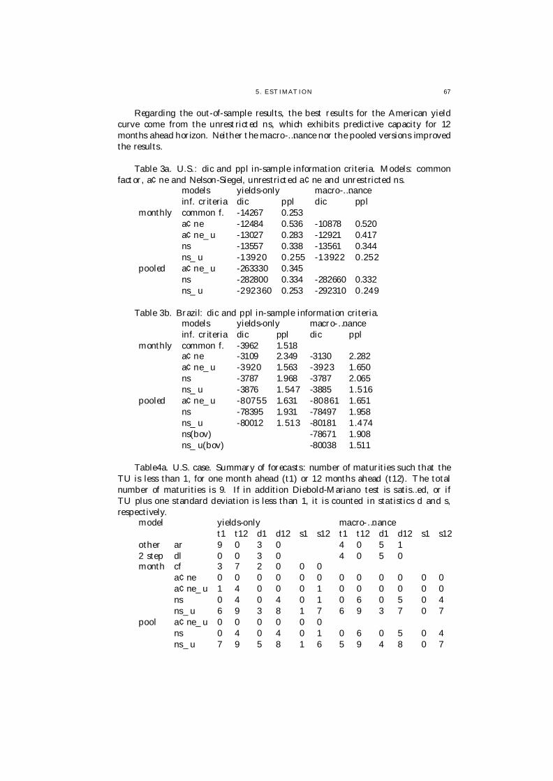
5 . EST IMAT ION 67
Regarding the out-of-sample results, the best results for the American yieldcurve come from the unrestricted ns, which exhibits predictive capacity for 12months ahead horizon. Neither the macro-…nance nor the pooled versions improvedthe results.
Table 3a. U.S.: dic and ppl in-sample information criteria. Models: commonfactor, a¢ne and Nelson-Siegel, unrestricted a¢ne and unrestricted ns.
models yields-only macro-…nanceinf. criteria dic ppl dic ppl
monthly common f. -14267 0.253a¢ne -12484 0.536 -10878 0.520a¢ne_u -13027 0.283 -12921 0.417ns -13557 0.338 -13561 0.344ns_u -13920 0.255 -13922 0.252
pooled a¢ne_u -263330 0.345ns -282800 0.334 -282660 0.332ns_u -292360 0.253 -292310 0.249
Table 3b. Brazil: dic and ppl in-sample information criteria.models yields-only macro-…nanceinf. criteria dic ppl dic ppl
monthly common f. -3962 1.518a¢ne -3109 2.349 -3130 2.282a¢ne_u -3920 1.563 -3923 1.650ns -3787 1.968 -3787 2.065ns_u -3876 1.547 -3885 1.516
pooled a¢ne_u -80755 1.631 -80861 1.651ns -78395 1.931 -78497 1.958ns_u -80012 1.513 -80181 1.474ns(bov) -78671 1.908ns_u(bov) -80038 1.511
Table4a. U.S. case. Summary of forecasts: number of maturities such that theTU is less than 1, for one month ahead (t1) or 12 months ahead (t12). The totalnumber of maturities is 9. If in addition Diebold-Mariano test is satis…ed, or ifTU plus one standard deviation is less than 1, it is counted in statistics d and s,respectively.
model yields-only macro-…nancet1 t12 d1 d12 s1 s12 t1 t12 d1 d12 s1 s12
other ar 9 0 3 0 4 0 5 12 step dl 0 0 3 0 4 0 5 0month cf 3 7 2 0 0 0
a¢ne 0 0 0 0 0 0 0 0 0 0 0 0a¢ne_u 1 4 0 0 0 1 0 0 0 0 0 0ns 0 4 0 4 0 1 0 6 0 5 0 4ns_u 6 9 3 8 1 7 6 9 3 7 0 7
pool a¢ne_u 0 0 0 0 0 0ns 0 4 0 4 0 1 0 6 0 5 0 4ns_u 7 9 5 8 1 6 5 9 4 8 0 7

68 4. FOREC AST ING THE YIE LD CURVE: C OM PARING M ODELS
Contrary to the U.S. case, for Brazil the models generally showed low predictivecapacity. The exceptions are the ns model with Bovespa, the Diebold-Li and ARmodels, all for the 6 months horizon.
The inclusion of the IBovespa substantially improved the long-term predictions,but not short term results. Also, macro-augmented and pooled versions result aresimilar to the standard monthly yields-only results.
Table4b. Brazilian case. Summary of forecasts: number of maturities suchthat the TU is less than 1, for one month ahead (t1) or 6 months ahead (t6). Thetotal number of maturities is 9. If in addition Diebold-Mariano test is satis…ed, orif TU plus one standard deviation is less than 1, it is counted in statistics d and s,respectively.
model yields-only macro-…nancet1 t6 d1 d6 s1 s6 t1 t6 d1 d6 s1 s6
other ar 0 0 0 0 0 5 0 22 steps dl 0 0 0 0 0 5 0 2monthly cf 0 2 0 0 0 0
a¢ne 0 0 0 0 0 0 0 0 0 0 0 0a¢ne_u 1 2 0 0 0 0 0 0 0 0 0 0ns 0 0 0 0 0 0 0 0 0 0 0 0ns_u 1 2 0 0 0 0 2 2 0 0 0 0
pooled a¢ne_u 0 0 0 0 0 0 0 0 0 0 0 0ns 0 0 0 0 0 0 0 0 0 0 0 0ns_u 0 0 0 0 0 0 0 0 0 0 0 0ns(bov) 0 8 0 8 0 5
5.1. TU. The graphs below exhibit the values of the Theil-U for the 9 yieldmaturities, {1,3,6,12,24,36,60,84,120}-month for U.S. and {1,2,3,6,9,12,18,24,36}-month for Brazil. We present the results for the ns and dl models, comparing theirspeci…cations.
Each model is represented by two curves: the lower curve is the TU minus onestandard deviation and the upper curve the TU plus one deviation. The pooled andthe aggregated models are compared for the one month and the 12 months aheadforecasts using the Brazilian and American yield curve.
Figure A contains the U.S. forecasts. In the …rst row, the Diebold-Li (dl) modelis compared to the pooled yields-only (dnsy) or macro-…nance (dnsr) models. Thelower row considers the aggregated version. In both bases, we see that for the onemonth horizon, dl and ns models are similar, but for the 12 months horizon thedl model is outperformed by the ns versions. It also can be seen that all modelsexhibit good predictive capacity.
Figure B treats the Brazilian case. In the …rst row, dl, the aggregated (nsy)and the pooled (dnsy) versions are compared for the one and 6 months aheadpredictions. In all cases, they are speci…ed as yields-only.
The second row shows the comparison about the choice of observed factor,IBovespa or in‡ation and output gap. It is seen that the only model with goodforecasts is the Nelson-Siegel with IBovespa for the 6-month horizon. The use ofmacro factors or pooled versions do not help to improve the low performance of theyields-only model.

5 . EST IMAT ION 69
Figure A. TU U.S.: Pooled x Aggregated.
1 3 6 12 24 36 60 84 1200.4
0.6
0.8
1
1.2
1.4
1.6
TU
US 1m-ahead pool
dl yo yo mf mf
1 3 6 12 24 36 60 84 1200.4
0.6
0.8
1
1.2
1.4
1.6US 1m-ahead aggr
dl yo yo mf mf
1 3 6 12 24 36 60 84 1200.4
0.6
0.8
1
1.2
1.4
1.6
maturities
TU
US 12m-ahead pool
dl yo yo mf mf
1 3 6 12 24 36 60 84 1200.4
0.6
0.8
1
1.2
1.4
1.6
maturities
US 12m-ahead aggr
dl yo yo mf mf
Figure 1
Figure B. TU BR: Macro-…nance x IBovespa.
1 2 3 6 9 12 18 24 360
0.5
1
1.5
2
2.5
3
3.5
TU
BR 1m-ahead yo
dl aggr aggr pool pool
1 2 3 6 9 12 18 24 360
0.5
1
1.5
2
2.5
3
3.5BR 1m-ahead mf, bov
dl mf mf bov bov
1 2 3 6 9 12 18 24 360
0.5
1
1.5
2
2.5
3
3.5
maturities
BR 12m-ahead yo
TU
dl aggr aggr pool pool
1 2 3 6 9 12 18 24 360
0.5
1
1.5
2
2.5
3
3.5
maturities
BR 12m-ahead mf, bov
dl mf mf bov bov
Figure 2
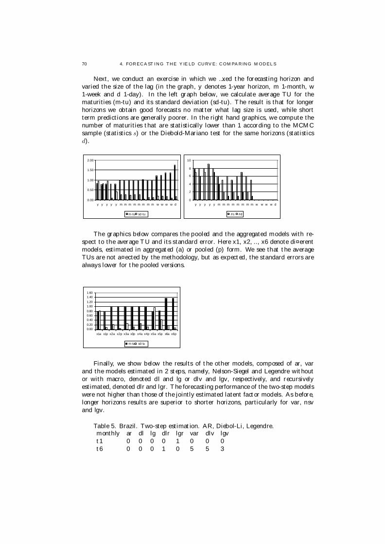
70 4. FOREC AST ING THE YIE LD CURVE: C OM PARING M ODELS
Next, we conduct an exercise in which we …xed the forecasting horizon andvaried the size of the lag (in the graph, y denotes 1-year horizon, m 1-month, w1-week and d 1-day). In the left graph below, we calculate average TU for thematurities (m-tu) and its standard deviation (sd-tu). The result is that for longerhorizons we obtain good forecasts no matter what lag size is used, while shortterm predictions are generally poorer. In the right hand graphics, we compute thenumber of maturities that are statistically lower than 1 according to the MCMCsample (statistics s) or the Diebold-Mariano test for the same horizons (statisticsd).
0.00
0.50
1.00
1.50
2.00
y y y y y m m m m m m m m w w w w d
m-tu sd-tu
0
2
4
6
8
10
y y y y y m m m m m m m m w w w w d
#s #d
The graphics below compares the pooled and the aggregated models with re-spect to the average TU and its standard error. Here x1, x2, .., x6 denote di¤erentmodels, estimated in aggregated (a) or pooled (p) form. We see that the averageTUs are not a¤ected by the methodology, but as expected, the standard errors arealways lower for the pooled versions.
0.00 0.20 0.40 0.60 0.80 1.00 1.20 1.40 1.60
x1a x1p x2a x2p x3a x3p x4a x4p x5a x5p x6a x6p
m-tu sd- tu
Finally, we show below the results of the other models, composed of ar, varand the models estimated in 2 steps, namely, Nelson-Siegel and Legendre withoutor with macro, denoted dl and lg or dlv and lgv, respectively, and recursivelyestimated, denoted dlr and lgr. The forecasting performance of the two-step modelswere not higher than those of the jointly estimated latent factor models. As before,longer horizons results are superior to shorter horizons, particularly for var, nsvand lgv.
Table 5. Brazil. Two-step estimation. AR, Diebol-Li, Legendre.monthly ar dl lg dlr lgr var dlv lgvt1 0 0 0 0 1 0 0 0t6 0 0 0 1 0 5 5 3

6. CO NC LUSION 71
The last table presents results for the Fama-Bliss database. It shows the resultsof yields-only 2 and 3 latent factor models (common factor and Nelson-Siegel), VARmodels, Diebold-Li model, ns and lg and macro-augmented versions nsv and lgv.
Table 6. Fama-Bliss: U.S. Latent factor, DL type models. 12 months aheadforecast.
Hor cf2 ns2 cf3 ns3 ar var ns lg nsv lgv dl3 0.77 1.05 0.94 1.35 0.96 1.31 1.39 0.71 0.85 0.75 0.7312 0.81 0.89 0.86 1.33 0.96 1.58 1.23 0.74 0.72 0.74 0.7036 0.79 0.94 0.79 1.37 0.80 1.73 1.46 0.75 0.83 0.80 0.7460 0.89 1.11 0.87 1.56 0.80 1.89 1.67 0.82 0.97 0.89 0.82120 1.20 1.47 1.17 1.97 1.41 2.46 2.06 0.93 1.16 0.98 0.93
6. Conclusion
Using MCMC, we estimated di¤erent classes of term structure models, in orderto compare the out-of-sample forecasts using American and Brazilian data.
“Pooled” versions of the macro-…nance models that combine daily yield dataand monthly macro data do not improve the forecasts, since their forecasts areequal on average to the standard models when there are su¢cient data, but theestimates and forecasts become more accurate.
The best model for the U.S. market was the unrestricted Nelson-Siegel. Eitherthe yields-only or the macro-…nance versions were similar in this case.
The use of IBovespa improved the latent factor models for Brazil for 6 monthsahead forecasts. DL models are easier to estimate, but the latent factor models,estimated in a more statistically sound way, showed at least as good results.


CHAPTER 5
Macro-Finance Models Combining Daily andMonthly Data
1. Introduction
The movements of the YC shape may reveal speci…c features about agents’expectations and in‡uences from macroeconomic and …nancial indicators. AfterAng and Piazzesi (2003) proposed a macro-…nance model incorporating economicindicators in a term structure model, a number of articles followed, notably Ang etal. (2007), Rudebusch and Wu (2004), Hördahl et al. (2006), Dewachter and Lyrio(2006), Diebold et al. (2006) and others.
This article aims to contribute to that literature in methodological and em-pirical aspects. We propose a method that combines monthly and daily data. Onthe empirical side, we analyze the dynamic properties of the models by means ofimpulse response functions and variance decompositions, which are calculated forAmerican and Brazilian markets.
We further propose an extension of the model that takes into account changesof regime on the reaction function of the yield curve to macroeconomic shocks.That is compared to an alternative way to accomplish the same task, by dividingthe sample into sub-samples corresponding to the possible regimes and comparingthe results. For example, in the Brazilian case, we test sub-samples correspondingto the president Cardoso after the adoption of the ‡oating exchange rate and thein‡ation-target regime, and president Lula starting in 2003.
For the U.S. sample, sub-samples corresponding to Greenspan or Bernanke aschairman of the Federal Reserve are compared. However, in this case we show thatthe data in the Bernanke sub-sample is insu¢cient for the estimation of our models.
The models used here can be classi…ed into two categories, the no-arbitrageand the econometric. In the …rst, the relation between the state variables andthe YC is derived considering that it is not possible to arbitrage from rates ofdi¤erent maturities. This condition introduce restrictions that reduce the numberof parameters at the cost of computationaly complicating the estimation.
In the econometric models, there are no such enforcements, but as Diebold andLi (2006) argues, if the data satis…es this condition and the model has good …tting,then this condition is indirectly met. In any case, the advantages and limitations ofeach approach, such as more formal rigor or clearer interpretation of the parameters,are empirically confronted here.
Once estimated, the models show the dynamic e¤ect of the identi…ed shocks onthe YC. We compare the behavior of very di¤erent markets: U.S. possesses longerand more stable data, while Brazil, have shorter available data which may alsoexhibit multiple regimes.
73

74 5. M AC RO-FINANC E MODELS COM BINING DAILY AND M ONT HLY DATA
In the macroeconomic literature, the forward versus backward looking approachis an unsolved issue in monetary policy theory (see Rudebusch and Wu, 2004). Themacro-…nance models, when combining macro variables and the YC, revisit thisquestion. Since the YC is composed of variables driven by expectations, a naturalway to include expectations into a dynamic macro model is to incorporate the YC.
As shown in the previous chapter, assuming an in…nite no-discount forward-looking policy justi…es for a¢ne models a restriction that is equivalent to considerthat the macro factors do not directly a¤ect the yield curve in the observationequation.
Macro and …nancial variables have di¤erent temporal unities. The former arenormally measured in monthly or quarterly frequency, which is the usual periodicityof the macro-…nance models. Thus, the models ignore the almost continuous-timedynamics of the …nancial variables. Also, in the monthly models, the intra-monthvariability of the daily variables is lost – by taking the monthly mean or selectingthe value observed for one day of the month –, with consequent loss of information.
We propose a “pooled” version of the macro-…nance model that avoids this yielddata, a feature that is particularly important for the case of developing marketswhich lack available samples.
The models were estimated with MCMC, with which we calculate informationcriteria that compare the performance of models with di¤erent degrees of complex-ity and number of parameters, and con…dence intervals of the impulse responsefunctions and variance decompositions.
Before the estimation of the models, we performed a simulation exercise, pre-sented in the Appendix. We tested the MCMC algorithm using the simulated dataand were able to recover the true parameters. Also, we calculate the Gelman-Rubinconvergence diagnostics of the Markov chains generated by the Gibbs sampling andMetropolis-Hastings algorithms.
2. Term Structure
Let us rewrite the general term structure equations
(2.1) Yt = A + BM Mt + Bθθt + σut , ut » N (0, In),
Mt = µM + ©MM Mt¡h + ©M θθt¡h + §MM εMt , εM
t » N (0,Ip),θt = µθ + ©θM Mt¡h + ©θθθt¡h + §θM εM
t + §θθεθt , εθ
t » N (0, Iq),substituting the time index t by the indices day d and month m .
Consider two alternatives for the observed factor: either it is collected withmonthly frequency, in which case equation (2.3) is used, or it is collected on a dailybasis, which corresponds to equation (2.2).
² Case where the observed factors M have daily frequency:
(2.2) Ymd = A + BM Mmd + Bθθmd + σumd, umd » N (0,In),
Mmd = µM + ©MM Mm¡1d + ©Mθθm¡1d + §MM εMmd, εM
md » N (0, Ip),
θmd = µθ + ©θM Mm¡1d + ©θθθm¡1d + §θM εMmd + §θθεθ
md, εθmd » N (0, Iq).
² Case where observed factors M have monthly frequency:
(2.3) Ymd = A + BM Mm + Bθθmd + σumd , umd » N (0, In),
Mm = µM + ©MM Mm¡1 + ©Mθθm¡1d + §M MεMmd, εM
md » N (0, Ip),θmd = µθ + ©θM Mm¡1 + ©θθθm¡1d + §θMεM
md + §θθεθmd , εθ
md » N (0,Iq),
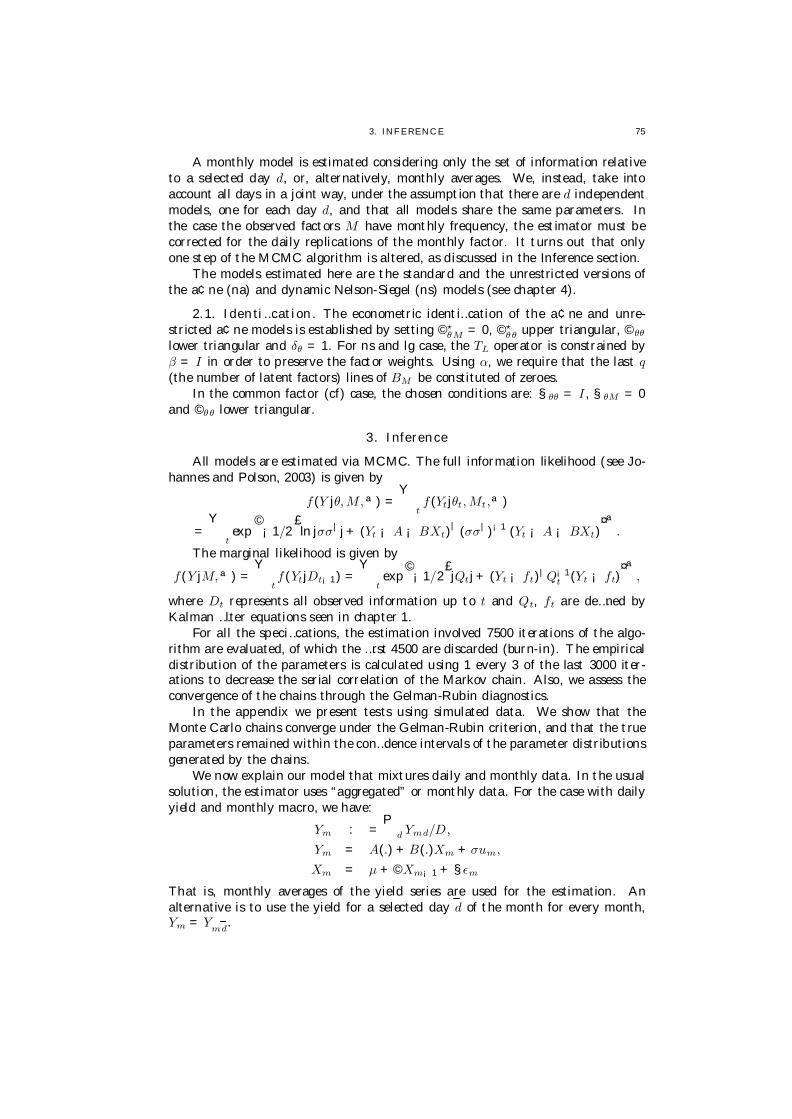
3. INFERENC E 75
A monthly model is estimated considering only the set of information relativeto a selected day d, or, alternatively, monthly averages. We, instead, take intoaccount all days in a joint way, under the assumption that there are d independentmodels, one for each day d, and that all models share the same parameters. Inthe case the observed factors M have monthly frequency, the estimator must becorrected for the daily replications of the monthly factor. It turns out that onlyone step of the MCMC algorithm is altered, as discussed in the Inference section.
The models estimated here are the standard and the unrestricted versions ofthe a¢ne (na) and dynamic Nelson-Siegel (ns) models (see chapter 4).
2.1. Identi…cation. The econometric identi…cation of the a¢ne and unre-stricted a¢ne models is established by setting ©?
θM = 0, ©?θθ upper triangular, ©θθ
lower triangular and δθ = 1. For ns and lg case, the TL operator is constrained byβ = I in order to preserve the factor weights. Using α, we require that the last q(the number of latent factors) lines of BM be constituted of zeroes.
In the common factor (cf) case, the chosen conditions are: §θθ = I , §θM = 0and ©θθ lower triangular.
3. Inference
All models are estimated via MCMC. The full information likelihood (see Jo-hannes and Polson, 2003) is given by
f (Y jθ, M, ª) =Y
tf (Yt jθt , Mt ,ª)
=Y
texp
©¡1/2
£ln jσσ| j + (Yt ¡ A ¡ BXt)
| (σσ| )¡1 (Yt ¡ A ¡ BXt)¤ª
.
The marginal likelihood is given by
f (Y jM, ª) =Y
tf (Yt jDt¡1) =
Ytexp
©¡1/2£jQt j + (Yt ¡ ft)| Q¡1
t (Yt ¡ ft)¤ª
,
where Dt represents all observed information up to t and Qt, ft are de…ned byKalman …lter equations seen in chapter 1.
For all the speci…cations, the estimation involved 7500 iterations of the algo-rithm are evaluated, of which the …rst 4500 are discarded (burn-in). The empiricaldistribution of the parameters is calculated using 1 every 3 of the last 3000 iter-ations to decrease the serial correlation of the Markov chain. Also, we assess theconvergence of the chains through the Gelman-Rubin diagnostics.
In the appendix we present tests using simulated data. We show that theMonte Carlo chains converge under the Gelman-Rubin criterion, and that the trueparameters remained within the con…dence intervals of the parameter distributionsgenerated by the chains.
We now explain our model that mixtures daily and monthly data. In the usualsolution, the estimator uses “aggregated” or monthly data. For the case with dailyyield and monthly macro, we have:
Ym : =P
d Ymd/D,Ym = A(.) + B(.)Xm + σum,Xm = µ + ©Xm¡1 + §εm
That is, monthly averages of the yield series are used for the estimation. Analternative is to use the yield for a selected day d of the month for every month,Ym = Ymd.

76 5. M AC RO-FINANC E MODELS COM BINING DAILY AND M ONT HLY DATA
Next, we transform a daily model into a sum of monthly models for each dayd, whose likelihood is L(ªd jDd), where Dd is the information set associated to dayd. We assume independence among the residues of each model, which allow thepartition of the full likelihood into day-d likelihoods,
L(ªjD) =X21
d=1L(ªjDd).
The sum has 21 terms, the average number of business days in a month. In thisway, we turn a daily model into 21 monthly models that are jointly estimated. Theestimations are made under the assumption that
ªd = ª.
This procedure can be used even for daily observed macro factors. In this case, thepooled version will be more precise than monthly models, because of the decreasedvariance of the estimator.
In the case the observed state factor has monthly frequency, we replicate theobserved factor 21 times for each day of the month. The new estimator has the samemean as the aggregated estimator, except that the variance must be corrected toaccount for the introduced repetitions. However, only sub-problem 1 of the MCMCalgorithm (see chapter 4) is a¤ected by the replicated macro data, speci…cally theparameter © of the transition equation of the observed variables. We correct thevariance of the distribution of sub-problem 1 as follows.
Estimator for day d:
E(b©md) =µ
M 0mMm M 0
mθmd(M 0
mθmd)0 θ0mdθmd
¶¡1 µM 0
mMm+1θ 0
mdMm+1
¶.
Pooled estimator: replicate Mmd = Mm8d. Stacking the equations for thed = 1..D days of the month, we have:
E(b©m) =µ
M 0mdMmd M 0
mdθmd(M 0
mdθmd ) Vd
¶¡1 µM 0
mdMm+1dθ 0
mdMm+1d
¶
=µ
DM 0mMm DM 0
mθm
(DM 0mθm)0 DV
¶¡1 µM 0
mdMm+1dθ 0
mdMm+1d
¶
=µ
M 0mMm M 0
mθm
(M 0mθm)0 V
¶¡1 µM 0
mMm+1
θ0mMm+1
¶= E(bb©m)
where bb©m is the monthly estimator and
Vd = θ 0mdθmd, V =
Pd Vd/D, θm =
Pd θmd/D.
That is, the mean of the pooled and of the aggregated estimators are equal. How-ever, the variances must be corrected by the factor D:
V (b©m) = σ2µ
DM 0mMm DM 0
mθm
(DM 0mθm)0 DV
¶¡1
= D¡1σ2µ
M 0mMm M 0
mθm
(M 0m θm)0 V
¶¡1
= D¡1V (bb©m),
whereσ2 =
Pmd(Mm+1 ¡ ©MM Mm ¡ ©Mθθmd)2/#(md).
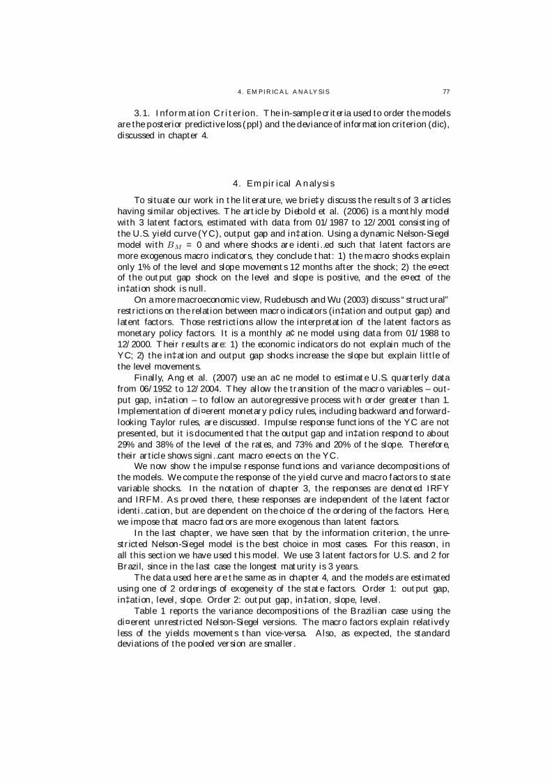
4 . EM PIR IC AL ANALYSIS 77
3.1. Information Criterion. The in-sample criteria used to order the modelsare the posterior predictive loss (ppl) and the deviance of information criterion (dic),discussed in chapter 4.
4. Empirical Analysis
To situate our work in the literature, we brie‡y discuss the results of 3 articleshaving similar objectives. The article by Diebold et al. (2006) is a monthly modelwith 3 latent factors, estimated with data from 01/1987 to 12/2001 consisting ofthe U.S. yield curve (YC), output gap and in‡ation. Using a dynamic Nelson-Siegelmodel with BM = 0 and where shocks are identi…ed such that latent factors aremore exogenous macro indicators, they conclude that: 1) the macro shocks explainonly 1% of the level and slope movements 12 months after the shock; 2) the e¤ectof the output gap shock on the level and slope is positive, and the e¤ect of thein‡ation shock is null.
On a more macroeconomic view, Rudebusch and Wu (2003) discuss “structural”restrictions on the relation between macro indicators (in‡ation and output gap) andlatent factors. Those restrictions allow the interpretation of the latent factors asmonetary policy factors. It is a monthly a¢ne model using data from 01/1988 to12/2000. Their results are: 1) the economic indicators do not explain much of theYC; 2) the in‡ation and output gap shocks increase the slope but explain little ofthe level movements.
Finally, Ang et al. (2007) use an a¢ne model to estimate U.S. quarterly datafrom 06/1952 to 12/2004. They allow the transition of the macro variables – out-put gap, in‡ation – to follow an autoregressive process with order greater than 1.Implementation of di¤erent monetary policy rules, including backward and forward-looking Taylor rules, are discussed. Impulse response functions of the YC are notpresented, but it is documented that the output gap and in‡ation respond to about29% and 38% of the level of the rates, and 73% and 20% of the slope. Therefore,their article shows signi…cant macro e¤ects on the YC.
We now show the impulse response functions and variance decompositions ofthe models. We compute the response of the yield curve and macro factors to statevariable shocks. In the notation of chapter 3, the responses are denoted IRFYand IRFM. As proved there, these responses are independent of the latent factoridenti…cation, but are dependent on the choice of the ordering of the factors. Here,we impose that macro factors are more exogenous than latent factors.
In the last chapter, we have seen that by the information criterion, the unre-stricted Nelson-Siegel model is the best choice in most cases. For this reason, inall this section we have used this model. We use 3 latent factors for U.S. and 2 forBrazil, since in the last case the longest maturity is 3 years.
The data used here are the same as in chapter 4, and the models are estimatedusing one of 2 orderings of exogeneity of the state factors. Order 1: output gap,in‡ation, level, slope. Order 2: output gap, in‡ation, slope, level.
Table 1 reports the variance decompositions of the Brazilian case using thedi¤erent unrestricted Nelson-Siegel versions. The macro factors explain relativelyless of the yields movements than vice-versa. Also, as expected, the standarddeviations of the pooled version are smaller.

78 5. M AC RO-FINANC E MODELS COM BINING DAILY AND M ONT HLY DATA
Table 1. Brazil. Variance decompositions 6 months after shock. Upper half: oneach column, contributions of shocks (s-gap, s-in‡, s-lev and s-slop) on the variationof the variables. Lower half: standard deviations of upper half.
resp: pooled order 1 resp: aggreg. order 1 resp: aggreg. order 2shock gap in‡ shrt long gap in‡ shrt long gap in‡ shrt longs-gap 0.69 0.05 0.03 0.01 0.59 0.07 0.12 0.03 0.70 0.05 0.03 0.01s-in‡ 0.07 0.70 0.08 0.05 0.08 0.64 0.11 0.12 0.06 0.70 0.08 0.05s-lev 0.05 0.22 0.32 0.93 0.09 0.25 0.30 0.83 0.22 0.02 0.78 0.12s-slop 0.19 0.03 0.57 0.01 0.24 0.04 0.47 0.03 0.02 0.23 0.11 0.82standard deviations-gap 0.07 0.03 0.03 0.01 0.13 0.04 0.12 0.03 0.07 0.04 0.02 0.01s-in‡ 0.04 0.08 0.04 0.02 0.05 0.08 0.11 0.07 0.04 0.08 0.04 0.01s-lev 0.04 0.08 0.07 0.02 0.08 0.08 0.18 0.09 0.07 0.02 0.06 0.01s-slop 0.06 0.02 0.06 0.01 0.10 0.03 0.16 0.03 0.02 0.08 0.05 0.02
Next, we present the impulse response functions of the unrestricted model in…gure I. The aggregated and pooled versions are compared in each graph. The rowspresent the responses of the in‡ation, short rate and slope to industrial output gap,in‡ation, level and slope shocks.
Instead of plotting the mean response, we plot the one deviation above responseand the one deviation below. In some cases the impulse response con…dence intervalof the pooled version is not contained on the con…dence interval of the aggregatedmodel, indicating that the pooled version may contain information that cannot bediscarded.
Table 2 shows that macro factors constitute important factors to explain theyield curve, specially the short yield. Likewise, the monetary factors explain animportant part of the macro factors, specially the industrial output gap.
Table 2. U.S. Variance decompositions 12 months after shock. Upper half:on each column, contributions of shocks (s-gap, s-in‡, s-lev, s-slop, s-curv) on thevariation of the variables. Lower half: standard deviations of upper half.
resp: pooled order 1 resp: aggreg. order 1 resp: aggreg. order 2shock gap in‡ shrt long gap in‡ shrt long gap in‡ shrt longs-gap 0.68 0.00 0.17 0.04 0.61 0.00 0.16 0.05 0.61 0.00 0.16 0.05s-in‡ 0.01 0.96 0.04 0.05 0.01 0.94 0.06 0.07 0.01 0.94 0.06 0.07s-lev 0.18 0.03 0.38 0.87 0.20 0.04 0.38 0.81 0.01 0.01 0.17 0.21s-slop 0.09 0.01 0.24 0.01 0.10 0.01 0.19 0.01 0.17 0.00 0.06 0.15s-curv 0.05 0.01 0.17 0.03 0.07 0.01 0.21 0.06 0.20 0.03 0.56 0.52standard deviations-gap 0.08 0.00 0.02 0.01 0.08 0.00 0.06 0.02 0.08 0.00 0.05 0.02s-in‡ 0.01 0.02 0.01 0.01 0.02 0.03 0.04 0.04 0.02 0.03 0.04 0.03s-lev 0.06 0.02 0.03 0.01 0.06 0.02 0.07 0.05 0.01 0.01 0.04 0.04s-slop 0.03 0.01 0.02 0.00 0.03 0.01 0.06 0.01 0.04 0.01 0.02 0.03s-curv 0.03 0.01 0.03 0.01 0.04 0.01 0.08 0.04 0.09 0.03 0.10 0.07
The pooled and the aggregated versions results are very similar. This resultindicates that the U.S. series is long enough, and so monthly data already producesaccurate results.

4 . EM PIR IC AL ANALYSIS 79
Continuing, we show in …gure II the impulse response functions of the unre-stricted Nelson-Siegel model with U.S. data. In all cases, the one deviation aboveand below impulse response functions of the pooled version is contained in the aggre-gated model con…dence interval. This means that both versions contain equivalentinformation, the only di¤erence being that the pooled is more accurate in somecases.
Figure I. Brazil. Impulse response. Thick line: pooled version. Thin line:aggregated version. We plot 95% con…dence bands around responses.
1st column: in‡ation resp. 2nd col.: short rate resp. 3rd col.: slope resp.output gap shock
-0.40
-0.20
0.00
0.20
0.40
0.60
0.80
1.00
1.20
1.40
1.60
1 2 3 4 5 6
-0.40
-0.20
0.00
0.20
0.40
0.60
0.80
1.00
1 2 3 4 5 6
-1.40
-1.20
-1.00
-0.80
-0.60
-0.40
-0.20
0.00
0.20
0.40
1 2 3 4 5 6
in‡ation shock
-2.00
-1.00
0.00
1.00
2.00
3.00
4.00
5.00
6.00
1 2 3 4 5 6
-0.60
-0.40
-0.20
0.00
0.20
0.40
0.60
0.80
1 2 3 4 5 6
-1.80
-1.60
-1.40
-1.20
-1.00
-0.80
-0.60
-0.40
-0.20
0.00
0.20
1 2 3 4 5 6
level shock
0.00
0.20
0.40
0.60
0.80
1.00
1.20
1.40
1.60
1.80
2.00
1 2 3 4 5 6
0.00
0.20
0.40
0.60
0.80
1.00
1.20
1.40
1.60
1 2 3 4 5 6
0.00
0.50
1.00
1.50
2.00
2.50
1 2 3 4 5 6
slope shock
-1.20
-1.00
-0.80
-0.60
-0.40
-0.20
0.00
0.20
0.40
0.60
1 2 3 4 5 6
-0.40
-0.20
0.00
0.20
0.40
0.60
0.80
1.00
1.20
1.40
1 2 3 4 5 6
-1.60
-1.40
-1.20
-1.00
-0.80
-0.60
-0.40
-0.20
0.00
0.20
1 2 3 4 5 6

80 5. M AC RO-FINANC E MODELS COM BINING DAILY AND M ONT HLY DATA
Figure II. U.S. Impulse response. Thick line: pooled version. Thin line: aggre-gated version. We plot 95% con…dence bands around responses.
1st column: in‡ation resp. 2nd col.: short rate resp. 3rd col.: slope resp.gap shock
-0.06
-0.04
-0.02
0.00
0.02
0.04
0.06
0.08
0.10
0.12
1 2 3 4 5 6 7 8 9 10 11 12
0 . 0 0
0 . 0 2
0 . 0 4
0 . 0 6
0 . 0 8
0 . 1 0
0 . 1 2
0 . 1 4
0 . 1 6
0 . 1 8
0 . 2 0
1 2 3 4 5 6 7 8 9 10 11 12
-0.14
-0.12
-0.10
-0.08
-0.06
-0.04
-0.02
0.00
0.02
1 2 3 4 5 6 7 8 9 10 11 12
in‡ation shock
0 . 0 0
0 . 5 0
1 . 0 0
1 . 5 0
2 . 0 0
2 . 5 0
3 . 0 0
1 2 3 4 5 6 7 8 9 10 11 12
0 . 0 0
0 . 0 1
0 . 0 2
0 . 0 3
0 . 0 4
0 . 0 5
0 . 0 6
0 . 0 7
0 . 0 8
0 . 0 9
0 . 1 0
1 2 3 4 5 6 7 8 9 10 11 12
-0.03
-0.02
-0.01
0.00
0.01
0.02
0.03
0.04
0.05
0.06
1 2 3 4 5 6 7 8 9 10 11 12
level shock
0 . 0 0
0 . 0 5
0 . 1 0
0 . 1 5
0 . 2 0
0 . 2 5
1 2 3 4 5 6 7 8 9 10 11 12
0 . 0 0
0 . 0 5
0 . 1 0
0 . 1 5
0 . 2 0
0 . 2 5
0 . 3 0
1 2 3 4 5 6 7 8 9 10 11 12
-0.10
-0.05
0.00
0.05
0.10
0.15
0.20
0.25
1 2 3 4 5 6 7 8 9 10 11 12
slope shock
-0.02
0.00
0.02
0.04
0.06
0.08
0.10
0.12
1 2 3 4 5 6 7 8 9 10 11 12
0 . 0 0
0 . 0 5
0 . 1 0
0 . 1 5
0 . 2 0
0 . 2 5
1 2 3 4 5 6 7 8 9 10 11 12
-0.20
-0.15
-0.10
-0.05
0.00
0.05
1 2 3 4 5 6 7 8 9 10 11 12
curvature shock
-0.10
-0.05
0.00
0.05
0.10
0.15
1 2 3 4 5 6 7 8 9 10 11 12
0 . 0 0
0 . 0 5
0 . 1 0
0 . 1 5
0 . 2 0
0 . 2 5
1 2 3 4 5 6 7 8 9 10 11 12
-0.20
-0.15
-0.10
-0.05
0.00
0.05
0.10
1 2 3 4 5 6 7 8 9 10 11 12
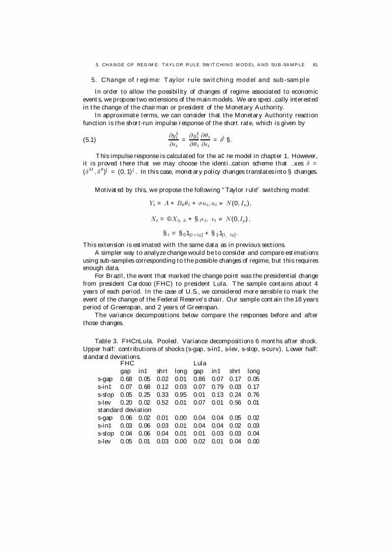
5. CHANGE OF REG IM E: TAYLOR RULE SW IT C HING M ODEL AND SUB -SAMP LE 81
5. Change of regime: Taylor rule switching model and sub-sample
In order to allow the possibility of changes of regime associated to economicevents, we propose two extensions of the main models. We are speci…cally interestedin the change of the chairman or president of the Monetary Authority.
In approximate terms, we can consider that the Monetary Authority reactionfunction is the short-run impulse response of the short rate, which is given by
(5.1)∂y1
t
∂εt=
∂y1t
∂θt
∂θt
∂εt= δ| §.
This impulse response is calculated for the a¢ne model in chapter 1. However,it is proved there that we may choose the identi…cation scheme that …xes δ =(δM , δθ)| = (0, 1)|. In this case, monetary policy changes translates into § changes.
Motivated by this, we propose the following “Taylor rule” switching model:
Yt = A + Bθθt + σut, ut » N (0, In),
Xt = ©Xt¡h + §tεt, εt » N (0,Ip),
§t = §01[t<t0] + §11[t¸t0] .
This extension is estimated with the same data as in previous sections.A simpler way to analyze change would be to consider and compare estimations
using sub-samples corresponding to the possible changes of regime, but this requiresenough data.
For Brazil, the event that marked the change point was the presidential changefrom president Cardoso (FHC) to president Lula. The sample contains about 4years of each period. In the case of U.S., we considered more sensible to mark theevent of the change of the Federal Reserve’s chair. Our sample contain the 18 yearsperiod of Greenspan, and 2 years of Greenspan.
The variance decompositions below compare the responses before and afterthose changes.
Table 3. FHCnLula. Pooled. Variance decompositions 6 months after shock.Upper half: contributions of shocks (s-gap, s-in‡, s-lev, s-slop, s-curv). Lower half:standard deviations.
FHC Lulagap in‡ shrt long gap in‡ shrt long
s-gap 0.68 0.05 0.02 0.01 0.86 0.07 0.17 0.05s-in‡ 0.07 0.68 0.12 0.03 0.07 0.79 0.03 0.17s-slop 0.05 0.25 0.33 0.95 0.01 0.13 0.24 0.76s-lev 0.20 0.02 0.52 0.01 0.07 0.01 0.56 0.01standard deviations-gap 0.06 0.02 0.01 0.00 0.04 0.04 0.05 0.02s-in‡ 0.03 0.06 0.03 0.01 0.04 0.04 0.02 0.03s-slop 0.04 0.06 0.04 0.01 0.01 0.03 0.03 0.04s-lev 0.05 0.01 0.03 0.00 0.02 0.01 0.04 0.00
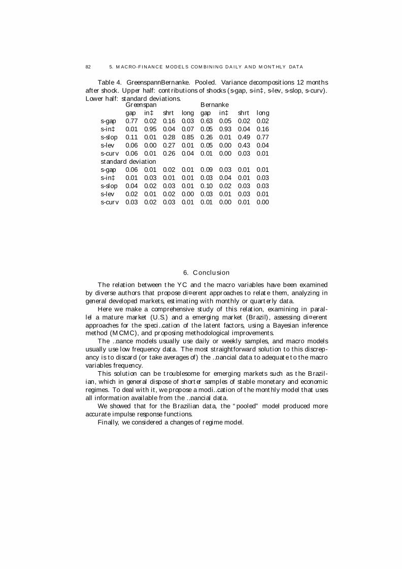
82 5. M AC RO-FINANC E MODELS COM BINING DAILY AND M ONT HLY DATA
Table 4. GreenspannBernanke. Pooled. Variance decompositions 12 monthsafter shock. Upper half: contributions of shocks (s-gap, s-in‡, s-lev, s-slop, s-curv).Lower half: standard deviations.
Greenspan Bernankegap in‡ shrt long gap in‡ shrt long
s-gap 0.77 0.02 0.16 0.03 0.63 0.05 0.02 0.02s-in‡ 0.01 0.95 0.04 0.07 0.05 0.93 0.04 0.16s-slop 0.11 0.01 0.28 0.85 0.26 0.01 0.49 0.77s-lev 0.06 0.00 0.27 0.01 0.05 0.00 0.43 0.04s-curv 0.06 0.01 0.26 0.04 0.01 0.00 0.03 0.01standard deviations-gap 0.06 0.01 0.02 0.01 0.09 0.03 0.01 0.01s-in‡ 0.01 0.03 0.01 0.01 0.03 0.04 0.01 0.03s-slop 0.04 0.02 0.03 0.01 0.10 0.02 0.03 0.03s-lev 0.02 0.01 0.02 0.00 0.03 0.01 0.03 0.01s-curv 0.03 0.02 0.03 0.01 0.01 0.00 0.01 0.00
6. Conclusion
The relation between the YC and the macro variables have been examinedby diverse authors that propose di¤erent approaches to relate them, analyzing ingeneral developed markets, estimating with monthly or quarterly data.
Here we make a comprehensive study of this relation, examining in paral-lel a mature market (U.S.) and a emerging market (Brazil), assessing di¤erentapproaches for the speci…cation of the latent factors, using a Bayesian inferencemethod (MCMC), and proposing methodological improvements.
The …nance models usually use daily or weekly samples, and macro modelsusually use low frequency data. The most straightforward solution to this discrep-ancy is to discard (or take averages of) the …nancial data to adequate to the macrovariables frequency.
This solution can be troublesome for emerging markets such as the Brazil-ian, which in general dispose of shorter samples of stable monetary and economicregimes. To deal with it, we propose a modi…cation of the monthly model that usesall information available from the …nancial data.
We showed that for the Brazilian data, the “pooled” model produced moreaccurate impulse response functions.
Finally, we considered a changes of regime model.
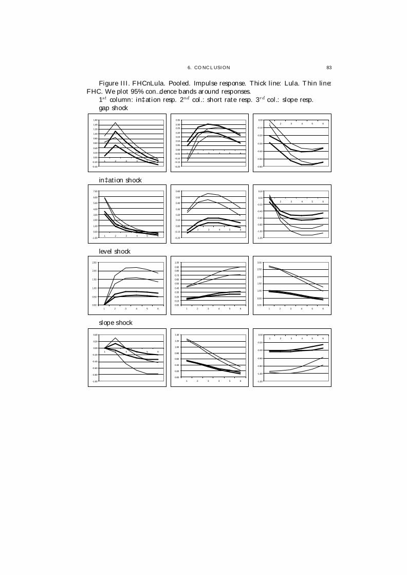
6. CO NC LUSION 83
Figure III. FHCnLula. Pooled. Impulse response. Thick line: Lula. Thin line:FHC. We plot 95% con…dence bands around responses.
1st column: in‡ation resp. 2nd col.: short rate resp. 3rd col.: slope resp.gap shock
-0.40
-0.20
0.00
0.20
0.40
0.60
0.80
1.00
1.20
1.40
1.60
1 2 3 4 5 6
-0.20
-0.15
-0.10
-0.05
0.00
0.05
0.10
0.15
0.20
0.25
0.30
0.35
1 2 3 4 5 6
-0.60
-0.50
-0.40
-0.30
-0.20
-0.10
0.00
1 2 3 4 5 6
in‡ation shock
-1.00
0.00
1.00
2.00
3.00
4.00
5.00
6.00
7.00
1 2 3 4 5 6
-0.20
-0.10
0.00
0.10
0.20
0.30
0.40
0.50
0.60
1 2 3 4 5 6
-1.20
-1.00
-0.80
-0.60
-0.40
-0.20
0.00
0.20
1 2 3 4 5 6
level shock
0.00
0.50
1.00
1.50
2.00
2.50
1 2 3 4 5 6
0.00
0.10
0.20
0.30
0.40
0.50
0.60
0.70
0.80
0.90
1.00
1 2 3 4 5 6
0.00
0.50
1.00
1.50
2.00
2.50
3.00
1 2 3 4 5 6
slope shock
-1.00
-0.80
-0.60
-0.40
-0.20
0.00
0.20
0.40
1 2 3 4 5 6
0.00
0.20
0.40
0.60
0.80
1.00
1.20
1.40
1 2 3 4 5 6
-1.20
-1.00
-0.80
-0.60
-0.40
-0.20
0.00
1 2 3 4 5 6
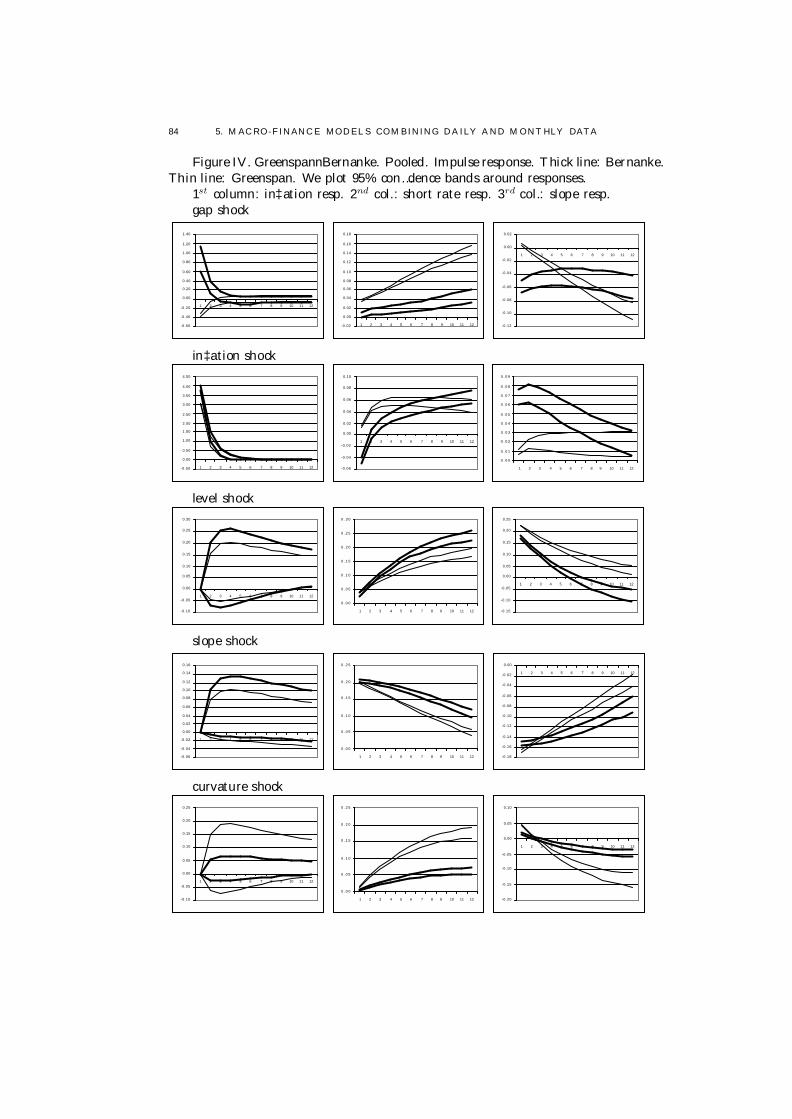
84 5. M AC RO-FINANC E MODELS COM BINING DAILY AND M ONT HLY DATA
Figure IV. GreenspannBernanke. Pooled. Impulse response. Thick line: Bernanke.Thin line: Greenspan. We plot 95% con…dence bands around responses.
1st column: in‡ation resp. 2nd col.: short rate resp. 3rd col.: slope resp.gap shock
-0.60
-0.40
-0.20
0.00
0.20
0.40
0.60
0.80
1.00
1.20
1.40
1 2 3 4 5 6 7 8 9 10 11 12
-0.02
0.00
0.02
0.04
0.06
0.08
0.10
0.12
0.14
0.16
0.18
1 2 3 4 5 6 7 8 9 10 11 12
-0.12
-0.10
-0.08
-0.06
-0.04
-0.02
0.00
0.02
1 2 3 4 5 6 7 8 9 10 11 12
in‡ation shock
-0.50
0.00
0.50
1.00
1.50
2.00
2.50
3.00
3.50
4.00
4.50
1 2 3 4 5 6 7 8 9 10 11 12
-0.06
-0.04
-0.02
0.00
0.02
0.04
0.06
0.08
0.10
1 2 3 4 5 6 7 8 9 10 11 12
0 . 0 0
0 . 0 1
0 . 0 2
0 . 0 3
0 . 0 4
0 . 0 5
0 . 0 6
0 . 0 7
0 . 0 8
0 . 0 9
1 2 3 4 5 6 7 8 9 10 11 12
level shock
-0.10
-0.05
0.00
0.05
0.10
0.15
0.20
0.25
0.30
1 2 3 4 5 6 7 8 9 10 11 12
0 . 0 0
0 . 0 5
0 . 1 0
0 . 1 5
0 . 2 0
0 . 2 5
0 . 3 0
1 2 3 4 5 6 7 8 9 10 11 12
-0.15
-0.10
-0.05
0.00
0.05
0.10
0.15
0.20
0.25
1 2 3 4 5 6 7 8 9 10 11 12
slope shock
-0.06
-0.04
-0.02
0.00
0.02
0.04
0.06
0.08
0.10
0.12
0.14
0.16
1 2 3 4 5 6 7 8 9 10 11 12
0 . 0 0
0 . 0 5
0 . 1 0
0 . 1 5
0 . 2 0
0 . 2 5
1 2 3 4 5 6 7 8 9 10 11 12
-0.18
-0.16
-0.14
-0.12
-0.10
-0.08
-0.06
-0.04
-0.02
0.00
1 2 3 4 5 6 7 8 9 10 11 12
curvature shock
-0.10
-0.05
0.00
0.05
0.10
0.15
0.20
0.25
1 2 3 4 5 6 7 8 9 10 11 12
0 . 0 0
0 . 0 5
0 . 1 0
0 . 1 5
0 . 2 0
0 . 2 5
1 2 3 4 5 6 7 8 9 10 11 12
-0.20
-0.15
-0.10
-0.05
0.00
0.05
0.10
1 2 3 4 5 6 7 8 9 10 11 12

APPENDIX A
Convergence
1. Description of Gelman-Rubin test
Below, we give the formulas associated to the Gelman-Rubin statistics:
Within chain variance:
W =1
m(n ¡ 1)
mX
j=1
mX
i=1
(xij ¡ xj )2.
Among chains variance:
B =n
m ¡ 1
mX
j=1
(xj ¡ x)2.
Estimated variance:
bV (x) = (1 ¡ 1n
)W +1n
B.
Gelman-Rubin statistics:
R =bV (θ)W
.
The Gelman-Rubin statistics R are applied to multiple chains. It indicatesconvergence when R is close to 1, below a certain critical level, for example, 1.1.
Details can be found in Robert and Casella (2005).
2. Simulation exercise
To validate our MCMC estimation algorithm, we simulate series using the unre-stricted Nelson-Siegel and a¢ne models, and test the performance of the estimatoron the series.
We show in the following that the algorithm successfully recovers the trueparameters. We simulate a sample of 1000 observations of a term structure withthe same maturities as the U.S. market. We show that the MCMC estimatesare close to the true parameters. Moreover, the true parameters stay within thecon…dence intervals of the estimated data.
Moreover, we apply the convergence diagnostics for the parameter chains gen-erated to estimate the above parameters.
For the Nelson-Siegel model, the results are given in Table A1.We further plot the Markov chains produced by the MCMC algorithm for
various parameters. For each parameter, 3 independent chains were run 3000 times.The results are given by Figures A1 to A4.
85

86 A . C ONVERGE NC E
In all cases the chains converged to its invariant measure around the true pa-rameter. We also compute the Gelman-Rubin statistics for the chains (some areomitted).
In Table A2, we plot the Markov chains produced by the MCMC algorithm forthe unrestricted a¢ne case. For each parameter, 3 independent chains were run3000 times. In all cases the chains converged to its invariant measure around thetrue parameter. Gelman-Rubin statistics are given (some are omitted), as well asthe convergence diagnostics of the parameter chains.
Table A1. Nelson-Siegel with 3 factors. True parameters, estimated parameters(mean and standard deviation of the parameter chains).
True Mean St. Dev.© 0.9 0.0 -0.1 0.87 0.02 -0.07 0.02 0.02 0.02
0.1 0.88 -0.1 0.12 0.87 -0.1 0.01 0.01 0.010.0 0.0 0.98 -0.01 0.00 0.98 0.01 0.01 0.01
V ¤ 105 3.6 -0.6 0.6 4.00 -0.34 0.46 0.09 0.03 0.03-0.6 1.0 -0.4 -0.34 1.01 -0.41 0.03 0.02 0.010.6 -0.4 1.8 0.46 -0.41 1.57 0.03 0.01 0.02
True Mean St. Dev.γ ¤ 102 7 6.99 0.05
A ¤ 102 True 5 5 5 5 5 5 5 5Estim 5.0 5.0 4.9 4.9 5.0 5.0 5.0 5.0St. Dev. - - - - - - - -
σu ¤ 104 True 4 4 4 4 4 4 4 4Estim 3.9 4.2 4.1 4.0 4.0 4.0 4.3 3.9St. Dev. 0.2 0.1 0.1 0.1 0.2 0.2 0.1 0.2
Figure A1. Nelson-Siegel with 3 factors.Chains of parameter γ.
500 1000 1500 2000 2500 30000.067
0.0675
0.068
0.0685
0.069
0.0695
0.07
0.0705
0.071
0.0715
iterations
gam
ma
data1data2data3
Gelman-Rubin test:R(γ) = [1.00, 1.00, 1.00]

2. SIMULATION EXERC ISE 87
Figure A2. Nelson-Siegel with 3 factors.Chains of parameter matrix ©.
0 1000 2000 30000.860.88
0.90.920.940.960.98
Phi
11
0 1000 2000 3000
-0.15-0.1
-0.050
0.05
0 1000 2000 3000-0.25
-0.2-0.15
-0.1-0.05
0 1000 2000 3000
0.060.08
0.10.120.14
Phi
21
0 1000 2000 3000
0.820.840.860.88
0 1000 2000 3000-0.14
-0.12
-0.1
-0.08
-0.06
0 1000 2000 3000-0.05
0
0.05
Phi
31
0 1000 2000 3000
-0.05
0
0.05
0 1000 2000 3000
0.920.940.960.98
11.02
Gelman-Rubin test:R(©11) = [1.00, 1.00, 1.00]R(©22) = [1.00, 1.00, 1.00]R(©33) = [1.00, 1.00, 1.00]
Figure A3. Nelson-Siegel with 3 factors.Chains of parameter matrix V.
0 1000 2000 3000
3.43.63.8
44.2
x 10-5
V11
0 1000 2000 3000-5-4
-3
-2
-1x 10
-6
0 1000 2000 3000
1
1.1
x 10-5
V22
0 1000 2000 3000
4
6x 10
-6
0 1000 2000 3000-5.2
-5-4.8-4.6-4.4-4.2
x 10-6
V32
0 1000 2000 3000
1.65
1.7
1.75
x 10-5
Gelman-Rubin test:R(V11) = [1.00, 1.00, 1.00]R(V22) = [1.00, 1.00, 1.00]R(V33) = [1.00, 1.00, 1.00]
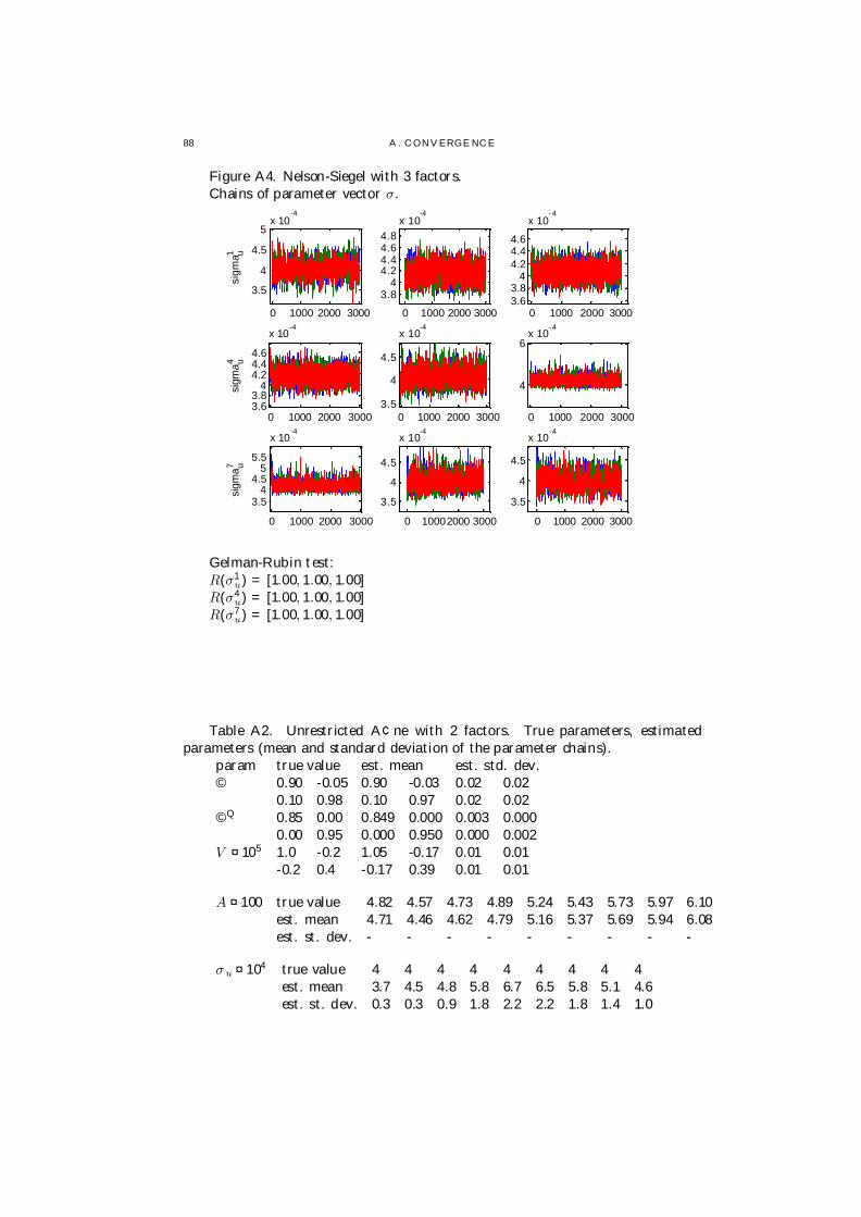
88 A . C ONVERGE NC E
Figure A4. Nelson-Siegel with 3 factors.Chains of parameter vector σ.
0 1000 2000 3000
3.5
4
4.5
5x 10
-4
sigm
a u1
0 1000 2000 3000
3.84
4.24.44.64.8
x 10-4
0 1000 2000 30003.63.8
44.24.44.6
x 10- 4
0 1000 2000 30003.63.8
44.24.44.6
x 10-4
sigm
a u4
0 1000 2000 30003.5
4
4.5
x 10-4
0 1000 2000 3000
4
6x 10
- 4
0 1000 2000 3000
3.54
4.55
5.5
x 10-4
sigm
a u7
0 10002000 3000
3.5
4
4.5
x 10-4
0 1000 2000 3000
3.5
4
4.5
x 10- 4
Gelman-Rubin test:R(σ1
u) = [1.00, 1.00, 1.00]R(σ4
u) = [1.00, 1.00, 1.00]R(σ7
u) = [1.00, 1.00, 1.00]
Table A2. Unrestricted A¢ne with 2 factors. True parameters, estimatedparameters (mean and standard deviation of the parameter chains).
param true value est. mean est. std. dev.© 0.90 -0.05 0.90 -0.03 0.02 0.02
0.10 0.98 0.10 0.97 0.02 0.02©Q 0.85 0.00 0.849 0.000 0.003 0.000
0.00 0.95 0.000 0.950 0.000 0.002V ¤ 105 1.0 -0.2 1.05 -0.17 0.01 0.01
-0.2 0.4 -0.17 0.39 0.01 0.01
A ¤ 100 true value 4.82 4.57 4.73 4.89 5.24 5.43 5.73 5.97 6.10est. mean 4.71 4.46 4.62 4.79 5.16 5.37 5.69 5.94 6.08est. st. dev. - - - - - - - - -
σu ¤ 104 true value 4 4 4 4 4 4 4 4 4est. mean 3.7 4.5 4.8 5.8 6.7 6.5 5.8 5.1 4.6est. st. dev. 0.3 0.3 0.9 1.8 2.2 2.2 1.8 1.4 1.0

2. SIMULATION EXERC ISE 89
Figure A5. Unrestricted a¢ne with 2 factors.Chains of parameter matrix ©Q.
500 1000 1500 2000 2500 3000
0.84
0.845
0.85
0.855
0.86
iterations
Phi
Q 1
500 1000 1500 2000 2500 3000
0.945
0.95
0.955
iterations
Phi
Q 2
data1data2data3
data1data2data3
Gelman-Rubin statistics:R(©Q
1 ) = [1.00, 1.02, 1.03]R(©Q
2 ) = [1.00, 1.05, 1.03]
Figure A6. Unrestricted a¢ne with 2 factors.Chains of parameter matrix ©.
0 1000 2000 30000.8
0.85
0.9
0.95
1
Phi
11
0 1000 2000 3000-0.1
-0.05
0
0.05
0.1
Phi
12
0 1000 2000 30000
0.05
0.1
0.15
0.2
Phi
21
0 1000 2000 30000.9
0.95
1
Phi
22
Gelman-Rubin statistics:R(©11) = [1.00, 1.01, 1.00]R(©22) = [1.00, 1.01, 1.01]

90 A . C ONVERGE NC E
Figure A7. Unrestricted a¢ne with 2 factors.Chains of parameter matrix V.
500 1000 1500 2000 2500 3000
9
10
11
x 10-6
V11
500 1000 1500 2000 2500 3000-3
-2
-1x 10
-6
V12
500 1000 1500 2000 2500 3000
3.54
4.55
x 10-6
V22
Gelman-Rubin statistics:R(V11) = [1.00, 1.02, 1.01]R(V22) = [1.00, 1.02, 1.01]
Figure A8. Unrestricted a¢ne with 2 factors.Chains of parameter vector σu.
0 1000 2000 3000
3
4
5
x 10-4
sigm
a u1
0 1000 2000 30003.5
4
4.5
x 10-4
0 1000 2000 300034567
x 10-4
0 1000 2000 3000
4
6
8
x 10-4
sigm
a u4
0 1000 2000 3000
2468
101214
x 10-4
0 1000 2000 30000
5
10
15x 10
-4
0 1000 2000 30000
5
10
15x 10
-4
sigm
a u7
0 1000 2000 30000
5
10
15x 10
-4
0 1000 2000 30000
5
10
15x 10
-4
R(σu1 ) = [1.00, 1.00, 1.03]
R(σu4 ) = [1.00, 1.00, 1.00]
R(σu7 ) = [1.00, 1.00, 1.00]

APPENDIX B
References
(1) Almeida, C., Duarte, A., Fernandes, C. (1998) Decomposing and simu-lating the movements of term structures in emerging eurobonds markets,Journal of Fixed Income, 1, 21–31.
(2) Almeida, C., Gomes, R., Leite, A., Vicente, J. (2007A) Movimentos daestrutura a termo e critérios de minimização do erro de previsão em ummodelo paramétrico exponencial, Working paper series 146, Central Bankof Brazil.
(3) Almeida, C., Gomes, R., Leite, A., Vicente, J. (2007B) Does curvatureenhance forecasting? Working paper series 155, Central Bank of Brazil.
(4) Almeida, C., Vicente, J. (2008) The role of no-arbitrage on forecasting:lessons from a parametric term structure model, forthcoming in Journalof Banking and Finance.
(5) Almeida, C. and J. Vicente (2009). Identifying volatility risk premia from…xed income Asian options. Journal of Banking and Finance, 33, p. 652-661.
(6) Amato, J., Luisi, M. (2006) Macro factors in the term structure of creditspreads, BIS Working Papers No. 203.
(7) Ang, A., Dong, S., Piazzesi, M. (2007) No-arbitrage Taylor rules, NBERWorking Paper 13448.
(8) Ang, A., Piazzesi, M. (2003) A no-arbitrage vector autoregression of termstructure dynamics with macroeconomic and latent variables, Journal ofMonetary Economics, 50, 745–787.
(9) Banerjee, S., Carlin, B., Gelfand, A. (2004) Hierarchical Modeling andAnalysis. for Spatial Data. CRC Press/Chapman Hall.
(10) Berndt, A., R. Douglas, D. Du¢e, M. Ferguson, and D. Schranzk (2004).Measuring default risk premia from default swap rates and EDFs. Work-ing Paper, Stanford University.
(11) Black, F. and Cox, J. (1976) Valuing corporate securities: some e¤ects ofbond indenture provisions, Journal of Finance, 31(2), 351–367.
(12) Black, F. and Scholes, M. (1973) The pricing of options and corporateliabilities, Journal of Political Economy, 81(3), 637–654.
(13) Bogdanski, J., Tombini, A., Werlang, S. (2000) Implementing In‡ationTarget in Brazil, Working Paper Series 1, Central Bank of Brazil.
(14) Chen, L.-H. (2001) In‡ation, real short-term interest rates, and the termstructure of interest rates: a regime-switching approach, Applied Econom-ics, 33(3), 393-400.
(15) Chen, R., Scott, L. (1993) Maximum likelihood estimation for a multi-factor equilibrium model of the term structure of interest rates, Journalof Fixed Income, 3, 14–31.
91
92 B. REFERE NC ES
(16) Collin-Dufresne, P., Goldstein, R., Jones, C. (2006) Identi…cation of max-imal a¢ne term structure models. Working paper.
(17) Cox, J., Ingersoll, J., Ross, S. (1985) A theory of the term structure ofinterest rates. Econometrica, 53: 385-407.
(18) Dai, Q., Philippon, T. (2004) Government de…cits and interest rates: ano-arbitrage structural VAR approach, Working paper.
(19) Dai, Q., Singleton, K. (2000) Speci…cation analysis of term structure ofinterest rates, Journal of Finance, 55, 1943–78.
(20) Davidson, R., MacKinnon, J. (1993) Estimation and inference in econo-metrics. New York: Oxford University Press.
(21) Dewachter, H., Lyrio, M. (2006) Macro Factors and the Term Structureof Interest Rates. Journal of Money, Credit and Banking, 38(1), 119–140.
(22) Diebold, F., Li, C. Forecasting the term structure of government bondyields. Journal of Econometrics, 130, 337-364.
(23) Diebold, F., Rudebusch, G., Aruoba, S. (2006) The macroeconomy andthe yield curve: a dynamic latent factor approach, Journal of Economet-rics, 131, 309–338.
(24) Diebold, F., Piazzesi, M., Rudebusch, G. (2005) Modeling bond yieldsin …nance and macroeconomics, American Economic Review, 95, N. 2,415–20.
(25) Du¤ee, G. (2002). Term premia and interest rates forecasts in a¢ne mod-els. Journal of Finance, 57, p. 405-443.
(26) Du¢e, D. (2001) Dynamic asset pricing theory, 3rd ed., Princeton: Prince-ton University Press.
(27) Du¢e, D., Kan, R. (1996) A yield-factor model of interest rates, Mathe-matical Finance, 6, 379–406.
(28) Du¢e, D., Pedersen, L., Singleton, K. (2003) Modeling sovereign yieldspreads: a case study of Russian debt, Journal of Finance, 58, 119-159.
(29) Du¢e, D. and Singleton, K. (1999) Modeling term structures of default-able bonds, Review of Financial Studies, 12, 687–720.
(30) Fachada, P. (2001) In‡ation targeting in Brazil: reviewing two yearsof monetary policy 1999/00, Working paper series 25, Central Bank ofBrazil.
(31) Fackler, P. (2000). Moments of a¢ne di¤usions, Working paper, NorthCarolina State University.
(32) Fraga, A., Goldfa jn, I., Minella, A. (2003) In‡ation targeting in emergingmarket economies, Working paper series 76, Central Bank of Brazil.
(33) Freitas, P., Muinhos, M. (2001) A simple model for in‡ation targeting inBrazil, Working paper series 18, Central Bank of Brazil.
(34) Gamerman, D., Lopes, H. (2006) Markov chain monte carlo: stochasticsimulation for Bayesian inference, 2nd Ed. London: Chapman & Hall.
(35) Gelfand, A., Ghosh, S. (1998) Model choice: a minimum posteriori pre-dictive loss approach. Biometrika, 85, 1-11.
(36) Ghezzi, P., Xu, D. (2002) From fundamentals to spreads. Deutsche BankGlobal Markets Research.
(37) Giesecke, K. (2004) Credit risk modeling and valuation: an introduction,in Credit Risk Models and Management Vol. 2, (Ed.) D. Shimko, Risk-books.

B. REFERE NC ES 93
(38) Goldfa jn, I., Werlang, S. (2000) The pass-through from depreciation toin‡ation: a panel study, Working paper series 5, Central Bank of Brazil.
(39) Goldman Sachs Global Economics Department (2007). BRICs and be-yond.
(40) Hamilton, J. (1994) Time Series Analysis, Princeton University Press.(41) Harvey, A. (1989) Forecasting, structural time series models and the
Kalman …lter. Cambridge University Press: Cambridge.(42) Hejazi, W. (2000) Yield spreads as predictors of industrial production:
expectations on short rates or term premia?, Applied Economics, 32, 945-51.
(43) Hördahl, P., Tristani, O., Vestin, D. (2002) A joint econometric modelof macroeconomic and term structure dynamics. European Central BankWorking Paper.
(44) Johannes, M., Polson, N. (2006) MCMC methods for continuous-time…nancial econometrics, in Handbook of Financial Econometrics (Ed.) Aït-Sahalia, Y, Hansen, L.
(45) Kalev, P., Inder, B. (2006) The information content of the term structureof interest rates, Applied Economics, 38(1), 33-45.
(46) Lando, D. (1998) On Cox processes and credit risky bonds, Review ofDerivatives Research, 2(2), 99–120.
(47) Laurini, M., Hotta, L. (2008) Bayesian extensions to diebold-li term struc-ture model, Ibmec working paper 74.
(48) Leippold, M., Wu, L. (2003) Estimation and design of quadratic termstructure models, Review of Finance, 7(1), 47–73.
(49) Leland, H. (1994) Risky debt, bond covenants and optimal capital struc-ture, Journal of Finance, 49 (4), 1213–1252.
(50) Leland, H., Toft, K. B. (1996) Optimal capital structure, endogenousbankruptcy and the term structure of credit spreads, Journal of Finance,50, 789–819.
(51) Litterman, R., Scheinkman, J. (1991) Common factors a¤ecting bondreturns, Journal Fixed Income, 1, 51–61.
(52) Longsta¤, F. (1989) A nonlinear general equilibrium model of the termstructure of interest rates, Journal of Financial Economics 23, 195–224.
(53) Ludvigson, S., Ng, S. (2007) Macro factors in bond risk premia, TheReview of Financial Studies, forthcoming.
(54) Kalev, P., Inder, B. (2006) The information content of the term structureof interest rates, Applied Economics, 38(1), 33-45.
(55) Merton, R. (1974) On the pricing of corporate debt: the risk structure ofinterest rates, Journal of Finance 29(2), 449–470.
(56) Minella, A., Freitas, P., Goldfa jn, I., Muinhos, M. (2003) In‡ation tar-geting in Brazil: constructing credibility under exchange rate volatility,Working paper series 77, Central Bank of Brazil.
(57) Moench, E. (2008) Forecasting the yield curve in a data-rich environment:a no-arbitrage factor-augmented VAR approach, Journal of Econometrics,146(1).
(58) Moody’s (2008). Sovereign default and recovery rates, 1983-2007, WorkingPaper, Moody’s Global Credit Research. Available at http://www.moodys.com/.
94 B. REFERE NC ES
(59) Muinhos, M., Alves, S. (2003) Medium-size macroeconomic model for theBrazilian economy, Working paper series 64, Central Bank of Brazil.
(60) Moreira, A., Rocha, K. (2004) Two-factor structural model of determi-nants of Brazilian sovereign risk, Journal of Fixed Income, 14(2).
(61) Nelson, C., Siegel, A. (1987) Parsimonious modeling of yield curves, Jour-nal of Business, 60, 4, 473-89.
(62) Pagès, H. (2001) Can liquidity risk be subsumed in credit risk? A casestudy from Brady bond prices, BIS Working Papers No 101.
(63) Pan, J. and K. Singleton (2008). Default and recovery implicit in theterm structure of sovereign CDS spreads. Journal of Finance, 63 (5), p.2345-2384.
(64) Pericoli, M., Taboga, M. (2006) Canonical term-structure models withobservable factors and the dynamics of bond risk premiums, Temi di Dis-cussioni, Banca D’Italia.
(65) Pinheiro, F., Almeida, C., Vicente, J. (2007) Um modelo de fatores la-tentes com variáveis macroeconômicas para a curva de cupom cambial,Brazilian Review of Finance, 5(1).
(66) Robert, C., Casella, G. (2005). Monte Carlo Statistical Methods. SpringerTexts in Statistics.
(67) Rodrigues, J., Araújo, F., Moreira, M. (2000) Optimal Interest Rate Rulesin In‡ation Targeting Frameworks, Working paper series 6, Central Bankof Brazil.
(68) Rudebusch, G., Wu, T. (2003) A macro-…nance model of the term struc-ture, monetary policy and the economy, Working Paper, Federal ReserveBank of San Francisco.
(69) Shiryaev, A. (1995). Probability, Springer Verlag.(70) Spencer, P. (2008). Stochastic volatility in a macro-…nance model of the
U.S. term structure of interest rates 1961–2004, Journal of Money, Creditand Banking, 40(6), 1177–1214.
(71) Spiegelhalter, D., Best, N., Carlin, B., van der Linde, A. (2002) Bayesianmeasures of model complexity and …t (with discussion). Journal of theRoyal Statistical Society Series B, 64, 583–639.
(72) Schönbucher, P. (2003) Credit Derivatives Pricing Models, Wiley Finance.(73) Shousha (2005). Estrutura a termo da taxa de juros e dinâmica macroe-
conômica no Brasil. Master’s dissertation, PUC-Rio.(74) Svensson, L. (1997) In‡ation forecast targeting: implementing and moni-
toring in‡ation targets. European Economic Review, 41, no. 6.(75) Vasicek, O. (1977). An Equilibrium Characterization of the Term Struc-
ture. Journal of Financial Economics, 5: 177-188.(76) Vicente, J., Tabak, B. (2008) Forecasting bond yields in the Brazilian …xed
income market. International Journal of Forecasting, 24(3), 490–497.(77) West, M., Harrison, J. (1997) Bayesian forecasting and dynamic models,
2nd ed., New York: Springer-Verlag.(78) Wu, T. (2003) Stylized facts on nominal term structure and business cy-
cles: an empirical VAR study, Applied Economics, 35(8), 901-906.