The Pennsylvania State University

The Graduate School

Department of Economics

ESSAYS ON RUSSIAN ECONOMIC GEOGRAPHY:

MEASURING SPATIAL INEFFICIENCY

A Thesis in

Economics

by

Tatiana N. Mikhailova

c© 2004 Tatiana N. Mikhailova

Submitted in Partial Fulfillmentof the Requirements

for the Degree of

Doctor of Philosophy

August 2004

The thesis of Tatiana Mikhailova has been reviewed and approved* by the following:

Barry W. IckesProfessor of EconomicsThesis AdvisorChair of Committee

N. Edward CoulsonProfessor of Economics

Eric BondProfessor of Economics

Regina SmythAssistant Professor of Political Science

Robert MarshallProfessor of EconomicsHead of the Department of Economics

*Signatures are on file in the Graduate School.

Abstract

Compared with other transition countries Russia faces the burden of extreme cold.This is not, however, strictly a function of geography. Soviet location policy directlyaffected the average (population weighted) temperature of the Russian economy. So-viet policy moved industry and population from the western part of the country tothe east, effectively making Russia even colder than it was in the pre-Soviet era.Movements to the east have the significant impact on aggregate temperature becausethe isotherms on the Eurasian continent resemble lines of longitude, not latitude.Thus, the Russian economy entering transition faces not only the usual burden of aninhospitable Russian climate, but also suffers from the extra disadvantage due to thelegacy of Soviet location policy.

In this thesis I estimate the cost to Russian economy of the inefficient spatial al-location of its productive resources. Spatial inefficiency can result not only in addedproduction and distribution costs — when regional comparative advantages are notexploited and unnecessary transportation and communication expenditures are in-curred — but also the wrong allocation of labor brings inefficiency in consumption:there are extra costs associated with people living in unsuitable places. In the Russiancontext, “unsuitable” usually means “too far” and “too cold.” I focus on the “costof cold,” or precisely, the cost of production being wrongly located in places with aclimate too cold.

The first essay is a counterfactual exercise. To obtain a benchmark of spatialefficiency, I construct an allocation of industry and population that would result inRussia in the absence of Soviet location policy. To design such an allocation, I imposeCanadian behavior on Russian initial conditions. I estimate a spatial dynamic modelon Canadian regional panel data in a multinomial logit framework. I then projectthe estimated relationship onto Russia. The result is a hypothetical allocation ofpopulation and industry, specific to Russia’s endowment and initial conditions, butfree of any disadvantages stemming from Russian historical circumstances.

This procedure, however, ignores the effect of WWII — a major exogenous shockto Russian economy with no precedent in Canada. We should expect that war wouldhave an impact on industry allocation irrespective of economic or political system.To account for the possible effects of WWII I conduct a separate simulation exercise,taking into account the fact that the war was fought primarily in the west. The resultsof this exercise show that the eastern part of Russia is still significantly overdeveloped— in other words, WWII explains only a small part of the misallocation.

iii

I construct an index of Temperature Per Capita (TPC) to capture the effect of lo-cation on aggregate temperature. Unlike other temperature indicators widely used inempirical growth literature, TPC is obtained by aggregating the temperature readingsnot over the territory, but over the population distribution. Thus, it provides moreinformative measure of temperature-related comparative advantages or disadvantagesof the economy, especially in short-run. I use the estimated allocation of populationto construct the counterfactual TPC. The comparison with the actual TPC revealsthat due to Soviet location policy Russia has become about 1.5◦C “colder.”

In the second essay I estimate the cost of cold directly. The most profound con-sequences of cold are extra energy use, added construction costs, health effects andproductivity loss. Using Russian regional data on energy use, health and productionI estimate the elasticity of each of these factors with respect to temperature. I thenuse these elasticities together with the TPC indices of the actual and the projectedallocation to estimate the extra burden of cold that resulted from the Soviet locationpolicy.

The results show strong and significant effect of cold on all the factors exam-ined. An increase in TPC of 1.5◦C would have improved aggregate health indicators:average infant mortality rate would have been 1.5% lower, country-wide aggregatemortality rate — at least 0.8% lower. The estimations for construction industry re-veal a 3.5% productivity loss in the actual allocation compared to the counterfactual.

The most significant impact of cold is on energy consumption. Cross-sectionalanalysis reveals that consumption of various kinds of energy by manufacturing pro-ducers increases 2.5 to 4% when January temperature drops 1◦C. Thus, 1.5◦C TPCdifference between the actual and counterfactual allocations translates into 3.5-6%industrial energy consumption increase country-wide. The similar results were ob-tained for the residential energy consumption: various estimates point on 6 to 9%total energy loss due to the misallocation of population. The cost of extra energyconsumption and the loss of construction productivity amount to 1.2% to 2.1% ofRussian GDP yearly.

iv

Contents

List of Tables vii

List of Figures viii

Acknowledgments ix

1 Introduction 1

2 Where Russians Should Live 42.1 Stylized facts . . . . . . . . . . . . . . . . . . . . . . . . . . . . . . . 42.2 The idea . . . . . . . . . . . . . . . . . . . . . . . . . . . . . . . . . . 82.3 The theoretical framework . . . . . . . . . . . . . . . . . . . . . . . . 112.4 Data description . . . . . . . . . . . . . . . . . . . . . . . . . . . . . 142.5 The procedure and the estimation results . . . . . . . . . . . . . . . . 14

2.5.1 Estimating the Canadian panel dynamic model . . . . . . . . 152.5.2 Estimation issues . . . . . . . . . . . . . . . . . . . . . . . . . 162.5.3 Projecting Canadian behavior onto the Russian data . . . . . 212.5.4 Accounting for WWII . . . . . . . . . . . . . . . . . . . . . . 242.5.5 Correction for the exogenous cross-regional fertility differences 272.5.6 Temperature per capita dynamics . . . . . . . . . . . . . . . . 302.5.7 Alternative criteria for model selection and robustness checks . 33

2.6 Conclusions . . . . . . . . . . . . . . . . . . . . . . . . . . . . . . . . 35

3 The Cost of the Cold 373.1 The Role of Climate . . . . . . . . . . . . . . . . . . . . . . . . . . . 373.2 Energy . . . . . . . . . . . . . . . . . . . . . . . . . . . . . . . . . . . 39

3.2.1 Energy use in producing sectors . . . . . . . . . . . . . . . . . 403.2.2 Residential energy consumption . . . . . . . . . . . . . . . . . 423.2.3 Cost . . . . . . . . . . . . . . . . . . . . . . . . . . . . . . . . 46

3.3 Productivity . . . . . . . . . . . . . . . . . . . . . . . . . . . . . . . . 493.3.1 Aggregate Production . . . . . . . . . . . . . . . . . . . . . . 503.3.2 Construction . . . . . . . . . . . . . . . . . . . . . . . . . . . 53

3.4 Health . . . . . . . . . . . . . . . . . . . . . . . . . . . . . . . . . . . 573.4.1 Mortality and morbidity . . . . . . . . . . . . . . . . . . . . . 57

v

3.4.2 What is the cost of the excess mortality? . . . . . . . . . . . . 613.5 Conclusions . . . . . . . . . . . . . . . . . . . . . . . . . . . . . . . . 63

Appendices

A Details of dataset construction 65A.1 Dependent variables: population and manufacturing employment . . . 65A.2 Regional characteristics . . . . . . . . . . . . . . . . . . . . . . . . . . 67

B Algorithm for choosing the optimal model 70

C Tables 72

Bibliography 86

vi

List of Tables

2.1 The results of the Monte-Carlo simulations for the projected Siberianpopulation: select distribution quantiles. . . . . . . . . . . . . . . . . 25

2.2 Excess population in Siberia and Far East, according to alternativeforecast models. . . . . . . . . . . . . . . . . . . . . . . . . . . . . . 36

3.1 Heating degree-days for select cities and Russia as a whole. . . . . . . 453.2 Savings of energy in counterfactual relative to actual allocation. . . . 463.3 Counterfactual “savings” of energy. . . . . . . . . . . . . . . . . . . . 483.4 Regional production function estimates (second stage). . . . . . . . . 513.5 Regional production function estimates, GRP deflated by subsistence

minimum index (second stage). . . . . . . . . . . . . . . . . . . . . . 533.6 Relative prices of construction output. . . . . . . . . . . . . . . . . . 543.7 Construction industry production function IV estimation. First stage. 553.8 Construction industry production function IV estimation. Second stage. 563.9 Production function estimates. Test of the robustness to the weighting. 563.10 Aggregate morbidity rate as a function of temperature. Robustness to

specification. . . . . . . . . . . . . . . . . . . . . . . . . . . . . . . . . 593.11 Aggregate mortality rate as a function of temperature. Robustness to

specification. . . . . . . . . . . . . . . . . . . . . . . . . . . . . . . . . 593.12 Standardized mortality rate as a function of temperature. . . . . . . . 603.13 Infant mortality rate as a function of temperature. . . . . . . . . . . . 62

A.1 Regional characteristics . . . . . . . . . . . . . . . . . . . . . . . . . . 68

C.1 Results of the restricted system estimation. Equations for population. 72C.2 Results of restricted system estimations. Equations for industry. . . . 73C.3 Projected vs actual population. Canada. . . . . . . . . . . . . . . . . 74C.4 Projected vs actual population. Russia. . . . . . . . . . . . . . . . . . 76C.5 The industrial structure control series. . . . . . . . . . . . . . . . . . 77C.6 Electricity in 1991. . . . . . . . . . . . . . . . . . . . . . . . . . . . . 78C.7 Electricity in 1992. . . . . . . . . . . . . . . . . . . . . . . . . . . . . 79C.8 Thermal energy in 1991. . . . . . . . . . . . . . . . . . . . . . . . . . 80C.9 Thermal energy in 1992. . . . . . . . . . . . . . . . . . . . . . . . . . 81C.10 Fuels in 1991. . . . . . . . . . . . . . . . . . . . . . . . . . . . . . . . 82C.11 Fuels in 1992. . . . . . . . . . . . . . . . . . . . . . . . . . . . . . . . 83

vii

List of Figures

2.1 Isotherms: average January air temperature. . . . . . . . . . . . . . . 52.2 Change in TPC index in Russia, Canada and USA. . . . . . . . . . . 72.3 Administrative divisions in the Russian Empire and the borders of the

Soviet Union and the Russian Federation. . . . . . . . . . . . . . . . 92.4 Major mineral resources in Russia and Canada. . . . . . . . . . . . . 102.5 Projected vs. actual population. Canada. . . . . . . . . . . . . . . . . 212.6 Projected vs. actual population. Russia. . . . . . . . . . . . . . . . . 232.7 Projected vs. actual population. Russia. Accounted for the impact of

WWII. . . . . . . . . . . . . . . . . . . . . . . . . . . . . . . . . . . . 282.8 Projected vs. actual population. Russia. Corrected for fertility differ-

ences. . . . . . . . . . . . . . . . . . . . . . . . . . . . . . . . . . . . 312.9 Projected vs. actual population. Russia. Accounted for the impact of

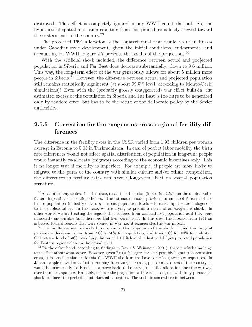
WWII and corrected for fertility differences. . . . . . . . . . . . . . . 322.10 Projected and actual TPC dynamics in Canada. . . . . . . . . . . . . 332.11 Projected and actual TPC dynamics in Russia. . . . . . . . . . . . . 342.12 Projected and actual TPC dynamics in Canada. Alternative models

compared. . . . . . . . . . . . . . . . . . . . . . . . . . . . . . . . . . 35

3.1 Energy sectors: consumption structure and counterfactual savings. . . 473.2 Gross regional product, prices and temperature. . . . . . . . . . . . . 52

viii

Acknowledgments

I would like to thank my advisor Barry W. Ickes for his guidance, invaluable adviceand encouragement. I am indebted to Herman Bierens, Eric Bond, Edward Coulson,Alexei Deviatov, Clifford Gaddy, Susumu Imai, Vijay Krishna, Joris Pinkse, ReginaSmyth and many workshop participants at Cornell University, SMYE ’02, MidwestEconomics Meeting, CEFIR, and Penn State for many helpful comments and discus-sions. I am grateful to Marjory Winn for her help with climatic data, and to YuriAndrienko, Yevgeniya Bessonova, and CEFIR for help and advice on Russian regionaldata. All errors are mine.

ix

Chapter 1

Introduction

More than a decade has passed since the collapse of the communist regimes in thecountries of Eastern Europe and USSR. The subsequent years of transition saw ex-amples of both success and difficulty in overcoming the legacy of economic distortionsinherited from the planned system. To what extent is the variation in economic per-formance among the transition countries determined by the initial conditions? Oneof the stylized facts of transition is that the countries where the legacy of the Sovietperiod was the deepest – the former USSR – experienced the largest drops in GDPand longer recessions. A part of the difference in performance is without a doubt at-tributable to the differences in policies. However, the role of initial conditions shouldnot be discounted.1

Among all transition economies Russian economy is among the most (if not themost) affected by the legacy of the Soviet regime. The focus of most researchers,however, has been mainly on structural and institutional distortions in Russia: al-location of production among sectors and industries and the absence of institutionsconductive to the market environment.

This work focuses on another feature of the initial conditions that sets Russia apart– geography. Russian geography is unique in two aspects: physical characteristics(size, climate, location) on one hand, and the extent of Soviet distortions in the spatialdimension on the other. Not only does Russia have an unfavorable geographicalendowment, but it also uses this endowment badly.

Russia’s position on the globe can hardly be characterized as favorable. In em-pirical cross-country studies of growth, findings generally reveal the positive role ofsuch characteristics of the geographical location as proximity to other markets, ac-cess to seashore, land quality and mild climate.2 Russian climatic conditions are

1Ultimately, policy design is endogenous to the initial conditions, because the very role of anypolicy in transition is to bridge the gap between the Soviet inheritance and free market, subject tothe (social, economic) constraints set by the same initial conditions.

2Gallup, Sachs & Mellinger (1999) conclude that both hot climate and location away fromseashore hinder economic performance. Bloom & Sachs (1998) point out the hot climate of CentralAfrica, responsible for disease transmission, as one of the factors hindering economic development.Rappaport & Sachs (2001) find a present-day positive productivity effect for the population growth

1

harsh, resources and population are dispersed over the vast territory, the few natu-ral transportation routes (rivers, seas) are located unfavorably for both internal andinternational trade, that leads to the prevalence of costly land transport. Naturalresources, though abundant, are located primarily far from population centers in theregions with most severe climate and least developed infrastructure. Russia’s sizeitself is a source of higher transaction costs: transportation and communications hasto reach over larger distances. All these factors drive production costs up, leavingRussia in absolute disadvantage.

The unfortunate geography of Russia and its impact on the economic performancehave been noted recently by Lynch (2002) and Parshev (1999). Russia’s problems,however, do not end with the poor overall geographical endowment. The spatialdistribution of economic activity inside present-day Russia carries the legacy of Sovietinvestment decisions – the geographical endowment is not being used efficiently.

In the field of economic geography, two fundamental factors are named as thedriving force behind the process of spatial allocation of economic activity – increas-ing returns to scale and location fundamentals.3 How important is each of thesefactors in reality is still unclear (Davis & Weinstein (2001)). It is normally presumed,however, that whenever these two forces are allowed to work freely, in the long runthe comparative advantages of the favorable locations are indeed being exploited.4

It is quite obvious that Russian economy presents a case when neither of thetwo forces were actually at work. In fact, in no other country in the world is thespatial allocation of industry as close to being exogenous as in Russia. The industrialstructure of the Soviet Union was produced by central planning, with investmentdecisions made in the absence of market prices. Taking into account that the economicefficiency objectives (if any) of the Soviet planning system were distorted by ideology,geopolitical concerns, military doctrines, historical circumstances, and other issuesspecific to the Soviet period, it is safe to expect that the existing spatial allocation ofthe productive resources in Russia is far from being optimal. More importantly, withRussia’s large size comes a wider margin of error: if economic activity is misallocated,it is more likely to be significantly misallocated, and, given Russia’s unfavorablegeography, such misallocations can be costly.

The present-day Russian economy bears not only the usual burden of the un-fortunate geographical location and climate, but as a direct result of Soviet locationpolicy, also suffers additional losses due to the inherited spatial inefficiency. But whileRussian geography cannot be changed, the spatial allocation of industry and peopleinside the country can be. Thus, there is room for policy.

in US counties located near seashores and navigable waterways.3See Fujita, Krugman & Venables (2000) (FKV) for collection and comprehensive analysis of the

models of spatial economy to date.4According to theoretical models in spatial economies (see FKV, for example) increasing returns

may result in multiplicity of spatial equilibria, and therefore even a market economy may be locked ina sub-optimal allocation. As far as reality is concerned, to the best of my knowledge the phenomenonof spatial suboptimality has not been observed and studied by researchers, save in the case of theformer Soviet block countries – in this instance being obviously due to policy intervention.

2

The challenge for policy analysis is associated with the following problem. Whilewe can almost certainly infer that Soviet system deviated from the optimal path ofspatial development, the extent of the distortion is not known until a counterfactualpath – a spatial development pattern that market forces would have produced –has been derived.5 And if this counterfactual path of spatial development is indeedsignificantly different from the Soviet history, then the next logical question is: “Whatis the economic cost of the Soviet distortions?”

This thesis is organized as follows. In chapter 2, I conduct a counterfactual exer-cise. I obtain the hypothetical counterfactual allocation of industry and populationthat would result in Russia under the market conditions and in the absence of Sovietlocation policy. Chapter 3 answers the second question: using the results in chapter2, I estimate the specific costs associated with Soviet spatial misallocations.

5The most prominent example of counterfactual analysis in economics is the classic work by Fogel(1964) on the importance of railroads for the American economy.

3

Chapter 2

Where Russians Should Live: ACounterfactual Alternative toSoviet Location Policy.

The history of Soviet location decisions can be characterized by a simple motto: “GoEast.” During the Soviet period, Siberia and Far East developed at a faster pace thanthe rest of the country, gaining in both share of population and share of industrialproduction. The massive movement of people to these regions, the places with mosthostile climates and away from existing population centers, has no precedent eitherin earlier history of Russia, or in any other country. As the direct result of theSoviet policy, a large share of present day Russian economy operates in unfavorableconditions: too far from the markets, too cold. Was the aggressive developmentof Siberia and the Far East inefficient from a market economy point of view? Theanalysis presented in this chapter aims to answer this question by building a market-based counterfactual pattern of spatial development in Russia.

This chapter is organized as follows. Section 2.1 discusses historical background:the features of Soviet location policy and the facts from transition period. Section 2.2describes the general idea and methodology. Section 2.3 gives the setup for the em-pirical part. Section 2.4 provides data description. Section 2.5 outlines the estimationprocedure and the results. Section 2.6 concludes.

2.1 Stylized facts

Throughout the course of the 20th century both population and industry in the USSRwere moved en masse from the west to the east, from European part of the countryto the regions east of Urals. The share of the total population living in Siberia andFar East increased from 5.5% in Russian Empire in 1910 to about 13% in the USSRin 1989.

Besides being remote and less developed, these regions are famous for extremelycold climates. The peculiar fact of the climatic geography of the Eurasian continent

4

Figure 2.1: Isotherms: average January air temperature.

is that isotherm lines resemble lines of longitude rather than latitude. Thus, in theprocess of populating Siberia, and even the Urals, people were moving across isothermlines: from warmer to colder places (see Figure 2.1).

After the breakup of the Soviet Union the new Russian state has received all ofthe regions with the most extreme climate under its jurisdiction, together with all theproblems associated. As a result, the economy inherited by Russia is probably themost distorted among the Newly Independent States, not only structurally but alsospatially.1 At the time of the collapse of the Soviet Union in 1991 the population ofSiberia and Far East reached 25% of Russian Federation’s total. No other country inthe world has such a high share of population living in climates so cold. For example,the population of Canadian Yukon and North-West territories, comparable in climateto Siberia, is only 0.3% of the total (1991).2

Temperature and economic growth

Does climate matter for economic performance? A common finding in the empiricalgrowth literature is that hot climates are bad for the economic growth, although thecauses of this empirical regularity are still being debated. For obvious reasons, onewould expect the cold climates to have a similar effect. Extreme cold is dangerous

1The majority of the defense industry was located in Russia. citeGaddy gives Russia’s share ofthe Soviet Union defense complex employment in 1985 as 71.2%, share of population as 51.8%.

2Canada is similar to Russia not just in climate, but also in the share of its territory that laysnorth of the Arctic Circle.

5

for the survival of the human species, thus it certainly has to be bad for the eco-nomic activity.3 Although it is possible to adapt to cold, this adaptation is costly:more energy is required for heating; productivity of both labor and machinery is de-creased; construction costs are multiplied due to extra material requirements, lowerproductivity, and quicker wear; the effect on people’s health is enormous.

So far, the adverse effect of cold on economic performance (either on level orgrowth) has not been studied very closely to date. There might exist several reasonswhy. First, data are limited: most of the growth studies either exclude Russia (orthe Soviet Union) from the dataset, or use the hardly reliable Soviet time data only.However, missing or mismeasuring this observation can prove crucial. Russia is notjust a cold country, but rather it is the cold country. By territorial temperatureaggregations Russia stands out as very cold even among other cold countries. Amap of the isotherms in Europe shows that Moscow has colder winters then evenNorwegian ports well above the Arctic Circle (see Figure 2.1).

Second, all of the empirical studies of temperature and growth use territorialaggregations of climate variables (temperature, or number of frost days, as Masters& McMillan (2000)). But what is important for the studies of economic activity iswhere the people actually live. According to the territorial temperature aggregationsthe countries of Northern Europe: Sweden, Norway, Finland appear to be cold. Infact, in these countries the population is concentrated along the seashores and in thesouth, where temperatures are not significantly different from the rest of Europe. Thesame is true for Canada, where people mainly live along the southern border.

As an alternative to the territorial temperature aggregations, Gaddy & Ickes(2001) propose the Temperature Per Capita (TPC) index.4 We can define TPCof country k as:

TPCk =∑

j

ηjτj , (2.1)

where ηj is the share of a country’s total population that resides in region j, and tjis the average mean temperature in region j. TPC is typically measured for a givenmonth – in most cases, January, the coldest month of the year. Regions are usuallybasic administrative units: provinces, oblasts, or states. In essence, TPC is a coun-trywide average temperature aggregated over the spatial distribution of population.Clearly, TPC for a country is not constant over time. If people migrate from colderto warmer places, TPC would rise. This way, a change in TPC serves as an index

3The evolutionary theory seems to be in accord with this: “Climate plays an important part indetermining the average number of a species, and periodical seasons of extreme cold or drought, Ibelieve to be the most effective of all checks ... In going northward, or in ascending a mountain,we far oftener meet with stunted forms, due to the directly [emphasis in original] injurious actionof climate, than we do in proceeding southwards or in descending a mountain.” – Charles Darwin,1859, Origin of the Species, Oxford World’s Classics ed. pp. 57-58.

4In a way, territorial temperature aggregations are measures of country’s climatic endowment.TPC describes how this endowment is used. Given the great degree of inertia in spatial popula-tion distribution, the latter is a more useful measure of climate-related comparative advantages ordisadvantages, especially in short-run.

6

Figure 2.2: Change in TPC index in Russia, Canada and USA.

measure of the climate-related effect of the spatial economic policy. This measureis especially useful in the case of Russia, as with Russian geographical endowment(alleged) spatial inefficiency is synonymous with cold.

In terms of TPC, especially its dynamics, Russia stands out even more. Not onlywas Russia colder than other countries at the beginning of the century, but also TPCin Russia fell even further through the Soviet years. While market economies weregradually warming up, with capital and labor resources allowed to freely migrate tothe more favorable locations, Russia got even colder (see Figure 2.2).

Soviet spatial policy: inefficient?

Of course, the fact that Eastern parts of Russia had been so aggressively developedduring Soviet times does not by itself prove that this was not economically efficient.One should not expect the regional distribution of industry to stay the same overtime. Remote regions should develop if and when technology makes it cost-effective.

Migration trends during the transition period exhibit the pattern opposite to thatof the Soviet times. This is but another evidence that the Eastern regions were“overdeveloped” during the Soviet times, and they host too many people and toomuch production from the market economy point of view. But even though thenegative net migration picture can pinpoint the most evident regional problems, itcannot show the degree of the misallocations. Positive net migration flow alone doesnot prove that a region is economically viable in long-run, but only shows that inshort-run there exists a region that performs even worse.5

Direct comparisons with other countries – Canada, Northern Europe – are alsoat best illustrative. Though the direction and scale of population movements in the

5Moreover, in short-run a poorly performing region may be locked in a poverty trap: people arecredit constrained and poor, and therefore, unable to move out.

7

Soviet Union have no precedent anywhere in the world, there are some importantissues to take into account.

First, the eastern regions of Russia are rich in natural resources. It could be ef-ficient to establish production near the primary inputs. Second, even at the timesof Russian Empire, Siberia was already populated, with several major cities estab-lished. Even if the location fundamentals were not favorable, the increasing returnsargument could validate the further development of Russian East. Third, it maybe strategically wise to populate the regions bordering historically unfriendly Chinaand Japan. Fourth, WWII was responsible for the destruction of infrastructure inthe western parts of the Soviet Union and for the shift of major defense industriesto Urals. Partly, this shift was due to political decisions of Soviet authorities, buteven without the political pressure we could expect to see similar effect in any kindof economy.

These considerations imply that the endowments and the unique historical circum-stances specific to Russia must be factored in to make an interesting counterfactual.To do so we must therefore simulate how Russia might have developed if market forceshad operated, and incorporate the special unique considerations mentioned above.

2.2 The idea

The idea for the simulation exercise is: use Canadian behavior as a benchmark of thespatial dynamics in market economy, but apply it to Russian initial conditions andendowment. Using Canadian data, estimate a model that characterizes the dynamiclinks between, on one hand, spatial structure of the economy and, on the other hand,initial conditions and regional characteristics. Then this model can be applied toRussia to produce the counterfactual “market” allocation.6

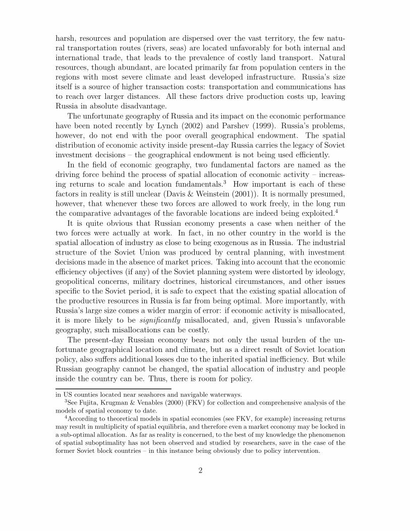
Why Canada? Applying the spatial dynamic relationships from one country ontoanother is most justified when the countries are similar in their endowments and stagesof development. Thus, the choice of Canada as a benchmark is relatively obvious:there is no other country in the world more close to Russia in climate and size.Both economies possess and export abundant natural resources. (Figure 2.4 showsthe geography of major mining operations in Canada and Russia.) Less obvious,but also important is the fact that both Russia and Canada at the beginning of thecentury had (and still have) the vast undeveloped amounts of land. Russia was still

6My concern is with the impact of Soviet location policy on the economic geography of RussianFederation, primarily on Siberia and Far East. However, for the most of the century Russia had beena part of the common market of the Soviet Union. In order to correctly account for the possibilityof the interregional migration, the projections must be applied to the whole territory of the SovietUnion. Thus, the dataset covers not only the present day Russian Federation but also some of theterritory that belongs now to other Newly Independent States. All regions that were part of boththe Soviet Union and Russian Empire are included. I apologize for using the term “Russia” to referto this artificial territorial entity throughout. I do this purely for the purpose of simplicity. Figure2.3 shows the administrative borders on the territory of the former Russian Empire and the formerUSSR.

8

Figure 2.3: Administrative divisions in the Russian Empire and the borders of theSoviet Union and the Russian Federation.

effectively expanding east, and Canada colonizing its west. Neither country seemedto be in long-run spatial equilibrium, but they were “moving in similar directions.”

At the same time, Canada is diverse enough to generate needed variance in thedata. For example, in Russia the coldest regions are also the most remote ones. InCanada, this is not true to the same degree. The city of Vancouver has the warmestclimate but located rather far from the most populous Toronto. Hopefully, this willallow us to effectively separate the two factors: cold and distance.

On the other hand, Canada has the benefit of much better access to oceans, andbetter natural water transportation network then Russia. Hence, due to the lowercosts of transportation, Canada is in a better position for both internal and inter-national trade. Canada also enjoys sharing the (only) international border with itsmajor trading partner, USA – a friendly neighbor and a large market. Russia, in con-trast, shares borders with an extremely diverse set of countries, and the relationshipswith the neighbors were uneasy at times. Among major trading partners of Russiaat the beginning of the century as well as now are Germany and United Kingdom,and shockingly none of the bordering states. While partly this situation might havedeveloped endogenously, either due to comparative advantage patterns, or (later) dueto the particular Soviet political choices, still any model estimated on Canadian datais likely to somewhat overstate the importance of geographical proximity for trade if

9

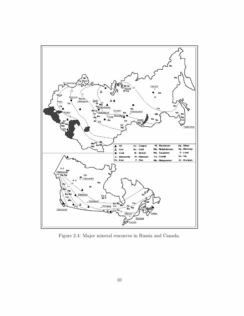
Figure 2.4: Major mineral resources in Russia and Canada.

10

applied to Russia.Another challenge in applying the Canadian model onto the Russian data lays

with the fact that Canadian regions are much more homogeneous then Russian oneswith respect to ethnic composition, human capital, and culture.7

I develop an empirical model of spatial population dynamics that is estimatedon Canadian regional data. The equations in general functional form link regionalpopulation growth to past population, industry, and various location characteristics.Then, the equations bearing the fitted values of the coefficients are applied to theRussian regional data for the initial (beginning of the century, before the OctoberRevolution) population and industry and the same set of regional characteristics. Theresult of the projections is the counterfactual allocation – specific to Russian startingpoint and geographical characteristics, but obtained using the dynamic relationshipfitted on market economy. The procedure is described in greater detail in Section 2.5.

Thus, the assumption behind the procedure is not that spatial structures of dif-ferent market economies should be similar, but rather that the dynamic forces thatimpact on location should be similar. In other words, we do not just compare theexisting spatial allocations in Russia and Canada, but instead we look at the changesin structure over time: initial conditions matter.

2.3 The theoretical framework

Consider a discrete-time setting with an infinite horizon where each period infinitelymany small agents, people, choose a location (i.e., a place to live) that maximizestheir utility. Simultaneously, firms choose locations that maximize expected profit.8

The people who have chosen a particular location compose the population in thislocation. The “amount” of industry in a location is characterized by total number ofemployed in manufacturing.

I model the spatial distribution of population and industry using the frameworkof the multinomial discrete choice (logit) model.9 Both indirect utility and profitfunctions are defined over the finite set of alternatives – locations. The locationchoices are obviously interdependent: people choose where to live taking into accountthe industry locations and other people’s decisions, and firms choose where to locatetaking into account locations of both population and other firms.

I use a reduced-form model. Utility in a location and potential profit depend onthe past values of population and the past values of industry employment as wellas on other exogenous characteristics of this location. Among these characteristics

7For example, we might expect based on cultural reasons alone a higher than average populationgrowth in Central Asian parts of the USSR. On average, family size has been traditionally larger inthose regions.

8Assume firms are economically small so that their decisions on location do not affect regionalprofitability.

9The application of multinomial logit model to the problems of location choice is a fairly standardapproach, pioneered by Carlton (1983).

11

are: temperature as a climate proxy, agricultural potential, natural resources, seaand rivers as natural transportation routes; infrastructure (man-built transportationnetwork), international trade routes as a proxy for the size of potential markets,agricultural potential, etc.

Assuming utility and profit functions are linear, write

uijt = βpopt ln POPj,t−1 + βind

t ln INDj,t−1 +

n∑k=1

βkt xk

j,t−1 + δujt + εu

ijt, (2.2)

πijt = αpopt ln POPj,t−1 + αind

t ln INDj,t−1 +n∑

k=1

αkt x

kj,t−1 + δπ

jt + επijt, (2.3)

where uijt is the utility of agent i in a location j in period t; POPj,t−1 and INDj,t−1

are, correspondingly, population and industrial employment in location j in periodt− 1; x1

j,t−1...xnj,t−1 are various characteristics of location j, possibly time-dependent;

δujt and δπ

j t – normal-distributed shocks to utility or profit specific to the location jand time t; εu

ijt and επijt – Weibull-distributed agent-location-time specific shocks to

utility or profit; α’s and β’s – parameters. The parameters of the utility and profitfunctions are time-dependent, so that the role of the different factors may change overtime.

Denote

ujt = βpopt ln POPj,t−1 + βind

t ln INDj,t−1 +n∑

k=1

βkt xk

j,t−1, (2.4)

ujt is a deterministic component of the utility function in a location j at time t. It iscommon to all agents. Also,

πjt = αpopt ln POPj,t−1 + αind

t ln INDj,t−1 +

n∑k=1

αkt x

kj,t−1, (2.5)

πjt is a deterministic and common to all agents component of the profit function.The probability that person i chooses location j at time t can be expressed as

P popijt = P

{ujt + δu

jt + εuijt > ult + δu

lt + εuilt|∀l

}=

∏l �=j

P{ujt + δu

jt + εuijt > ult + δu

lt + εuilt

}, (2.6)

and the probability that firm i chooses location j at time t is

P indijt = P

{πjt + δπ

jt + επijt > πlt + δπ

lt + επilt|∀l

}=

∏l �=j

P{πjt + δπ

jt + επijt > πlt + δπ

lt + επilt

}, (2.7)

12

Under the assumption that the ε’s are independent Weibull-distributed randomvariables, these probabilities take the following form:10

P popjt =

eujt+δujt∑L

l=1 eult+δult

, (2.8)

and

P indjt =

eπjt+δπjt∑L

l=1 eπlt+δπlt

. (2.9)

One can show that the observed shares of population and employment convergeto the above values (equations (2.8) and (2.9)) as number of agents in the economyincreases. Let Spop

jt be the observed share of population, Sindjt – be the observed share

of employment, then setting Spopjt = P pop

jt , Sindjt = P ind

jt and taking natural logarithmsof both sides, get

lnSpopjt = ujt + δu

jt − ln

(L∑

l=1

eult+δult

), (2.10)

and

ln Sindjt = πjt + δπ

jt − ln

(L∑

l=1

eπlt+δπlt

). (2.11)

Now consider the difference between log-shares in any two locations j,l:

ln Spopjt − ln Spop

lt = ujt − ult + ξujt, (2.12)

andln Sind

jt − ln Sindlt = πjt − πlt + ξπ

jt, (2.13)

where ξujt = δu

jt − δult and ξπ

jt = δπjt − δπ

lt- zero-mean normal variables.

Taking into account a loss of one degree of freedom due to the fact that∑L

l=1 Spoplt =∑L

l=1 Sindlt = 1, assume that SL is fixed and exclude location L from the sample. Ig-

noring the common denominator, and substituting the expressions (2.4) and (2.5) forujt and πjt get the equations to be estimated:

ln POPjt = β0t + βpop

t ln POPj,t−1 + βindt ln INDj,t−1 +

n∑k=1

βkt xk

j,t−1 + ξujt, (2.14)

ln INDjt = α0t + αpop

t ln POPj,t−1 + αindt ln INDj,t−1 +

n∑k=1

αkt x

kj,t−1 + ξπ

jt. (2.15)

The system (2.14) and (2.15) is estimated on the panel dataset.

10The assumption that εijt are independent is necessary for probabilities to have simple functionalform. In reality, we could expect that the individual unobservable shocks are correlated in spatialdimension: if a person prefers a particular location, possibly locations near it are also more attractiveto him on average.

13

2.4 Data description

I assembled a panel dataset to use in the estimations for Canada, and for the pro-jections onto Russia, from the various Canadian and Russian population census pub-lications, statistical yearbooks, and various maps.11 The panel dataset for Canadacontains data for population for 9 time points, one in every decade, starting withyear 1911 and up to year 1991. Data for industrial employment are available for year1911 and for years 1941-1991, for 1921 and 1931 data are missing. For 1921-1931 cen-sus publications give industry data only for cities of population greater than 15,000,but not for census districts. These years were dropped from the sample for industryequation, or replaced by 1911 data in in population equations for 1931 and 1941.

Data for the year 1981 are not included into census publications, but availablefrom Statistics Canada.12 Unfortunately, due to confidentiality issues, several smallmonoindustrial census districts are not listed. Thus, the quality of data available for1981 is substantially lower.

For each year the sample consists of 37 or 38 (upon inclusion of Newfoundland intoCanada) observations. The dependent variables are: population (POPj,t) and man-ufacturing industry employment (INDj,t) in a region. The set of independent vari-ables {xk

jt} includes the following regional characteristics (time and location subscriptsare omitted): area (AREA), mean January temperature (TEMP ), distance to thelargest city (DISTCAP ), number of railroads (RR), natural resources dummy vari-ables (OIL, COAL, METALS, TIMBER), and geographical characteristics dum-mies such as presence of trade route (R ABROAD), access to waterways (PORT ),quality of land (FARMING), and urbanization rate at the beginning of the century(URBAN). Appendix A has detailed information on the data sources.

For Russia, the dependent variables (population, industry employment) are col-lected for only two years: the starting year, 1910, and the final year, 1989. The 1910data will be used for the projections, as a starting point, and the 1989 data will beused for the actual vs. counterfactual comparison. The set of Russian regional char-acteristics is the same as for Canada, and data are collected for all the years presentin Canadian dataset. The sample size (number of regions included) for each year forRussia is 79.

Appendix A gives further details on data.

2.5 The procedure and the estimation results

This section describes the empirical procedure. The course of action can be outlinedin four steps.

11For more information on data sources and the details of the dataset construction, see AppendixA.

12“Manufacturing Industries of Canada: Geographical Distribution,” Regional and Small BusinessStatistics Section, Manufacturing and Primary Industries Division, Statistics Canada, 1982.

14

Step 1 Estimate the dynamic panel model for Canada to obtain the fitted values of themodel parameters.

Step 2 Project the estimated relationship onto Russian data. The result is the coun-terfactual spatial population distribution (not accounting for WWII).

Step 3 Incorporate the WWII effect into the projections.

Step 4 Correct the projections for the exogenous inter-regional fertility differences.

The counterfactual spatial population distributions obtained in steps 2, 3 and 4can be used to construct counterfactual TPC indices.

The following subsections describe the above steps in greater detail and reportthe results.

2.5.1 Estimating the Canadian panel dynamic model

The system of equations (2.14) and (2.15) is estimated on the Canadian panel data.The subscript (t−1) indicates value taken in the preceding time period in the dataset(10-year lagged).13

All parameters (α’s and β’s) in the equations (2.14) and (2.15) have a time sub-script t attached, indicating time-dependence. In general, the parameters can changeover time, reflecting possible changes in technology, world prices, tastes, or otherfactors that can impact on location choice.

Since the coefficients are allowed to freely vary with time, the system should beestimated time period-by-time period rather than together as a panel.14 However,the equations (2.14) and (2.15) represent, in essence, seemingly unrelated regressions.The error terms for industry and population in the same region and the same time areobviously correlated: a positive shock to region’s population is likely to coincide withsimilar shock in manufacturing employment. Thus, the equations (2.14) and (2.15)have to be estimated together with the use of Generalized Least Squares method.15

13Missing industry series for 1921 and 1931 were substituted by 1911 series.14A serious deficit of the degrees of freedom might arise when estimating 15 parameters on a

sample of 36 or 37 observations for each year. The number of degrees of freedom in each individualregression is 22 at best. Thus, the standard error estimates might not be reliable. It is desirable toimpose restrictions on the model: drop some variables from the regression to reduce the number ofparameters and release several degrees of freedom.

15As long as the set of explanatory variables is the same for industry and population regressions,the GLS estimation is equivalent to the simple OLS estimation of separate year-by-year regressions.The equivalence of GLS and OLS does not hold anymore, if (non-matching) restrictions are imposedon the parameters in these equations.

15

2.5.2 Estimation issues

The unobservable location-specific shocks

What if the set of explanatory variables ({POPt−1, INDt−1, xt−1})is not exhaustive?What if there exist other (unobservable) factors that impact on location?

Formally, if true relationship between population at time t and explanatory vari-ables includes an unobservable location-specific shock ηu

l,t, the equation (2.14) becomes

ln POPj,t = β0t + βpop

t ln POPj,t−1 + βindt ln INDj,t−1 +

n∑k=1

βkt xk

j,t−1 + ηul,t + ξu

jt, (2.16)

where ηujt may be correlated with other explanatory variables. In particular, if ηu

jt

terms are persistent across time dimension, then they are inevitably correlated withpast population levels lnPOPj,t−1. If a correctly specified relationship is given by theequation 2.16, but instead the equation (2.14) is estimated by OLS, the estimatedcoefficients would carry the omitted variable bias:

E[βt] = βt + γt, (2.17)

where βt is a vector of the coefficients. γt is a vector of the coefficients in a (cross-sectional) regression of ηt on the explanatory variables:

ηt = γ0t + γpop

t POPt−1 + γindt INDt−1 +

n∑k=1

γkt xk

j,t−1 + et. (2.18)

The presence of location-specific unobservables is common for cross-country orregional panel models.16 Normally, when the goal is to estimate the structural pa-rameters in a panel data setting the unobservables are integrated into location-specific(fixed or random) effects. In our case, however, the goal is different. We need to finda forecast model that would be relevant for counterfactual Russia. Obviously, thelocation-specific effects estimated on Canadian data cannot be transferred onto Rus-sia. Moreover, if a forecast is to be unbiased, the equation (2.14) estimated by OLSis the one to be used. Formally, the conditional expectation of population tomorrowas a function of explanatory variables is

E[POPt|POPt−1, INDt−1, xt−1] = β0t + βpop

t POPt−1 + βindt INDt−1

+n∑

k=1

βkt xk

j,t−1 + E[ηut |POPt−1, INDt−1, xt−1], (2.19)

where

E[ηut |POPt−1, INDt−1, xt−1] = γ0

t +γpopt POPt−1 +γind

t INDt−1 +n∑

k=1

γkt xk

j,t−1. (2.20)

16See Islam (1995) for the discussion of the common estimation issues in panel models of growth.

16

Substituting (2.20) into (2.19), get

E[POPt|POPt−1, INDt−1, xt−1] = (β0t + γ0

t ) + (βpopt + γpop

t )POPt−1

+ (βind + γindt )tINDt−1 +

n∑k=1

(βkt + γk

t )xkj,t−1 (2.21)

Under the assumption that the equation (2.18) correctly specifies the relationshipbetween unobservable location characteristics and observable explanatory variables,the parameters of a conditional expectation function given by the equation (2.21) areexactly what the OLS estimation of (2.14) gives. Under the key premise that (pre-communist and later counterfactual) Russia and Canada share all features of spatialdynamics – i.e. regional characteristics, observable or unobservable, have the sameimpact on location choices – this relationship gives unbiased Russian forecast.

Choosing the best model

Different restrictions imposed on the model coefficients in equations (2.14) and (2.15)can potentially lead to different results when projecting the Russian counterfactual.In essence, we are faced with a problem of choosing the best forecast model.

There exist two objectives in a model choice problem. First, an essential featureof a good model is the absence of systematic spatial bias. If one group of regions issystematically over- or underestimated in the Canadian model, the projected Russianallocation will most likely be biased as well. Second, we would like to minimize theunsystematic error – produce the highest quality forecast.

A model with too few explanatory variables would not fit the Canadian dynamicsclosely enough, and, consequently, give poor forecasts. A model with too manyvariables would give a better fit for every time period. But it may not give a betterfit for the 1911-1991 period as a whole. A good model should explain the long-termand general trends well and ignore the transitory and localized shocks. With toomany variables included there is a danger of overfitting the individual time periods.Overfitting not only makes estimators inefficient, it also records all the local andtransitory variations as if they were permanent and part of the long-term trend.Intuition suggests that the best forecast will result neither from the most parsimoniousnor from most exhaustive model, but from an “intermediate” case: some variablesare dropped from regressions.

A careful choice of variables for the earlier years is more crucial, as the projectionerror incorporated early in the process might grow in magnitude with each step (timeperiod) as forecast equations are applied recursively. Since it is unclear if the errorsfrom different time periods would accumulate or cancel each other out, we cannot sim-ply apply one of the widely used forecast model selection criteria (R-square adjusted,Akaike or Schwartz) to each time period individually - this would not guarantee thebest forecast for the final year.

Instead, the fit of any model may be evaluated in following way. First, estimatethe model. Second, apply the same procedure as planned for Russian projections,

17

only to Canada itself, working from 1911 data on. Then, compare the projectedvalues with real Canadian data for 1991 using some criterion. This exercise wouldshow how well the particular model fits the Canadian spatial dynamics overall.17

First and foremost, the Canadian projection errors should be examined (subjec-tively, at least) for any visible spatial bias. If the differences between projected andactual population values do not appear spatially random, the model is likely biasedand should not be used for the Russian projections.

Second, the in-sample (Canadian) forecast error must be evaluated numerically.Several criteria can be proposed to compare different models. I use the sum of rela-tive (weighted by the actual population) squared differences between the actual andprojected populations in 1991:

∑l

(POP Actual

l,1991 − POP Projl,1991

POP Actuall,1991

)2

. (2.22)

Of all possible models (i.e. subsets of explanatory variables) I choose the one that min-imizes the equation (2.22). My motivation was to choose the criterion that is focusedon the terminal period distribution and does not overlook the “small” low-populatedregions – the Canadian North, as this work is focused mostly on the implications forits Russian counterpart – Siberia and the Far East. Thus, weighting the errors byregion’s population is necessary to guarantee equal treatment of all regions. Onlyfinal year errors are taken into account.18

Intuitively, the criterion (2.22) looks for the model with negative intertemporalcorrelation in error terms. If the errors for the same region in different time periodsare negatively correlated, then in the projection process, when equations are appliedsequentially, errors in different time periods tend to cancel each other out rather thanadd up over time. Hence, the final year error is smaller.

In our case, the errors for the same region and different time periods turn out tobe positively correlated (at the level of 0.5 to 0.6 for different time period pairs inunrestricted model).19 Thus, the procedure is in fact looking for the model with thelowest positive intertemporal correlation in the residuals.

Ideally, the search for the best model would involve estimating the projected Cana-dian population for all possible models, and then selecting the model that minimizes(2.22). However, with 14 explanatory variables for each period and for each depen-dent variable, the number of possible combinations is astronomical – 214∗(9+7) = 2224

17Essentially, I am choosing the model that gives the best in-sample forecast. It might not betrue in general that best in-sample (Canadian) model would also give best out-of-sample (Russian)projections. But this the nature of a counterfactual exercise.

18Alternatively, instead of equation (2.22) other criteria could have been used. For example, otherweighting schemes (or none) could have been used, or forecast error could be evaluated along thewhole time path, not only in final period. Section 2.5.7 further discusses other criteria for modelselection, compares performance of different models, and checks the robustness of the main results.

19Due to, of course, the presence of the persistent unobservable location characteristics as discussedabove.

18

possible models. Estimating such a number of panel models is impossible – there isnot enough time. To find the best model, instead of a direct search I use an algo-rithm that searches through models eliminating variables one by one. The algorithmis described in Appendix B.

Results

Tables C.1 and C.2 (Appendix C) present the estimation results for the best (byweighted SSE criterion (2.22)) model.

In the population equation, the lagged population values are significantly positiveand stable over time; coefficients have a value slightly less than one, except for twoperiods: 1921 and 1991.20 The AREA coefficient is mostly positive as well. Thissuggests that a process of spatial population distribution is diffusing ceteris paribus:people tend to spread over the territory over time rather than concentrate in largeagglomeration points. This pattern is quite probable for the countries going throughthe territorial expansion, or as in cases of Russia and Canada, settling the sparselypopulated territories.

Lagged industrial employment is also positive and significant for the middle partof the century. The coefficient in 1921 is, in contrast, negative, while the coefficients in1931, 1941, and 1991 are close to zero. The zero coefficient in 1991 may be explainedby poor 1981 employment data quality. 1931 and 1941 equations use 1911 data forpast industry instead of missing 1921 and 1931 – so the variation in coefficients isexpected. As an alternative explanation, the 1911 to 1941 time period covers alsotwo major historical events: the massive migration to the Western provinces and theGreat Plains at the beginning of the century and The Great Depression of the 1930s.Thus, the near zero or negative coefficients for lagged industrial employment andtemperature might reflect population movement away from industrial centers and tothe regions with colder climates.21

The natural resources variables might have either positive or negative influence onpopulation growth. The presence of natural resources may draw people and industryinto the region, offering cheaper production inputs. Or alternatively, the monoindus-trial resource-oriented regions may grow slower ceteris paribus. The initial populationboom after the discovery of the resource might follow with a period of relatively slowpopulation growth, giving the negative sign to the lagged resource variable. Evi-dently from the results, the presence of natural resources seems to be of relatively

20The near-unity coefficient of past population is expected. In the presence of the unobservedtime-persistent regional idiosyncrasies evident in my case, the coefficient of past population tends tobe biased upward from a true structural value and (in case of diffusing process) towards unity. Thecoefficient of past population reflects not only dependence on past population per se, but also on allthe unobserved factors that determined population in the past. The unobservables are “built into”the past population. When interpreting the coefficients, one should bear in mind that the estimatedcoefficients are not true structural parameter values, thus do not reflect true causality.

21In addition to these considerations, it is not always possible to correctly compare the coefficientvalues between time periods simply due to the fact that for different time periods different sets ofvariables are be included into the equations.

19

little influence for the population distribution. Timber in 1921 and Metals in 1941have positive coefficients - these are the only exceptions.

The variables that proxy for trade possibilities, communications and the size ofthe reachable market (number of railroads, route abroad and ports) – presumablyadvantageous characteristics – do not appear to have a significant impact on thepopulation distribution dynamics either. Most likely, the positive influence of thesefactors is already built into the past population levels, and does not warrant higherthan average ceteris paribus population growth during XXth century. Urbanizationrate in 1911 has a consistently positive coefficient, suggesting that areas that weresettled and urbanized prior to the beginning of the century continued to attract peopleat a higher than average rate. Interestingly enough, in many time periods temperatureitself is not a significant explanatory variable – the movement of population towardswarmer areas is explained well enough by other factors.

The results for the industry regression follow roughly the same pattern, except fora few key distinctions. First, the role of lagged population and industry variables arereversed: lagged industry is now the more important factor. Second, infrastructureand/or access to markets seems to be slightly more important for industry, as thenumber of railroads has positive and significant coefficient for two time periods. Third,area does not always have strongly positive coefficient, and lagged industry coefficientsfor different years are both under and over 1. Thus, it is not clear whether industrialemployment does follow the same diffusion-type spatial dynamics as population.

The natural resources variables have predominantly negative or near-zero coeffi-cients, (coefficients for metal mining operations are significantly negative) suggestingthat primary industries in a region are not a magnet for other industrial production,but may even crowd it out.

In general, the results suggest that overwhelmingly the most important factorthat determines the spatial distribution of population (or industry) today is the pre-vious population (or industry) distribution. The spatial patterns of both populationand industry look very stable.22 Among less important factors, infrastructure, com-munication, transportation routes, access to markets tend to either promote fasterpopulation and industry growth or have insignificant dynamic impact. Natural re-sources do not make a region significantly more attractive for either population ormanufacturing industries.

Projecting the estimated model onto Canadian data from 1911 on allows us toproduce Figure 2.5 (and Table C.3). As the map shows, the positive and negativeerrors are distributed fairly evenly across the territory. There is no immediatelyvisible bias against or for any particular part of the country.

The model does worse predicting the population in large metropolitan areas. Sev-eral regions with major cities (Vancouver, Toronto, Montreal, Edmonton) have beengrowing fast during the century and have strongly positive unexplained error – ac-tual population is seriously higher than projected. The other large cities (Winnipeg,

22Most likely, because attractive features of locations manifested themselves through history: bestlocations are the ones most densely settled.

20

Numbers show the absolute difference between projected and actual population, in thou-sands.

Figure 2.5: Projected vs. actual population. Canada.

Halifax, Ottawa, etc) have either negative or near zero error. On average, however,the population of the biggest metropolitan areas is underestimated.

2.5.3 Projecting Canadian behavior onto the Russian data

I now use the estimated model to produce the counterfactual. Using the data onthe initial conditions and the exogenous characteristics for Russian regions, we applyequations (2.14) and (2.15) to Russian population (POP ) and industry (IND) data in1910, and all exogenous information to get the projected regional values of populationand industry employment in the next year in the panel. Formally,

ln POP RusProj1921 = βRus

1921 + βpop1921 lnPOP1911 + βind

1921 ln IND1911 +∑

k

βk1921x

k1911,

(2.23)

and

ln INDRusProj1941 = αRus

1941 + αpop1941 ln POP1931 + αind

1941 ln IND1911 +∑

k

αk1921x

k1911.

(2.24)

21

Note that the constant terms βRus and αRus are not equal to the intercepts in theequations (2.14) and (2.15), respectively, estimated on the Canadian data. Since themultinomial logit model describes the relationship between relative shares of differentregions in a total population of a country, and the shares have to sum up to 1,one degree of freedom is lost to that additional condition. In the same way, whenprojecting the model onto Russia, to properly calculate the relative shares of all theprovinces we need to account for the loss of one degree of freedom. Therefore, thevalues of βRus

t and αRust can be obtained from the condition:

∑79l=1 POP RusProj

l,t =

POP RusActualt , where POP RusActual

t is actual total population of the Soviet Union inyear t.23

In the next step I use the projected 1921 values of population in Russian regionsand 1910 industry data as an input for the 1931 population equation. The results arethe population estimates for 1931. Then, population in 1941 is projected in similarway. The projections for industry start with year 1941 as a function of 1931 projectedpopulation and 1910 actual industry data. Then, the forecast equation for the year1951 takes both industry and population 1941 projected values as arguments. Theprocedure is repeated until the year 1991.

The 1991 results present an alternative spatial allocation for Russia that wouldhave occurred if its development followed the Canadian path. This is the counterfac-tual allocation sought after: it is free of all the shocks and disadvantages specific toRussian history.

The counterfactual regional population levels are reported in the Table C.4, Ap-pendix C. The difference between actual and counterfactual population levels isplotted on the map on Figure 2.6.

The east-west divide is evident on the map. As the rule, the projected values ofpopulation in the western provinces are higher than the actual, and in the easternpart – lower than the actual. The degree of spatial autocorrelation is astonishing:all of the underdeveloped regions are located in the western part of the country.In the European part of the Former Soviet Union, the only four observations with apredicted population distinctly lower than actual are Moscow, Estlyandskaya province(now independent state of Estonia), Ekaterinoslavskaya province (home of Donbasscoal mining region) and Tavricheskaya (Crimean peninsula).

In the European part of the country, generally, the provinces around larger cities(St. Petersburg, and also the capitals of the Union Republics: Kiev, Minsk) experi-ence less of a population deficit in per capita terms. The population of Moscow isunderpredicted. The fast growth of Moscow in XXth century owes to its status as thecapital of the Soviet Union. At the turn of the century Moscow was only the secondlargest city in the Russian Empire.

The fact that Central Asian regions show a lot of excess population can be ex-

23It is not necessary to obtain the value of the constant term for each year. Since the relationshipbetween past and present population (or industry) is linear in logs, the constant added to all theobservations does not change the relative “weight” of different regions. Only the terminal-yearconstant term is of interest.

22

plained by cultural reasons: the fertility rates in Central Asia and parts of Caucasusare historically higher than in the rest of the country. I attempt to correct for thesedifferences later.

The eastern regions: Siberia, and especially the Far East are noticeably overpop-ulated. Even though the predicted number for the Siberian population is very high– about 19 million people (compare with 80,000 in Canadian Yukon and North-WestTerritories), it still leaves an astonishing 14.6 million of excess population east ofUrals. Moreover, the situation in neighboring regions of Urals is no better: they areoverpopulated as well.

Numbers show the absolute difference between projected and actual population, in thou-sands.

Figure 2.6: Projected vs. actual population. Russia.

Of course, the mere fact that predicted population for individual regions appear tobe over- or under- the actual level does not necessarily imply the general inefficiencyof the allocation. Forecast model is not 100% precise. Values for the most of theregional characteristics (temperature, distance, railroads, etc) used in the estimationsand projections are taken at the point of the regional (provincial) population center,but population is spread over the territory. Population levels for the individual regionsare very sensitive to the location of the borders. If a large city is located near a

23

regional border, a small change in administrative division might lead to big changesin population numbers. Thus even a spatial allocation reasonably close to efficientmight have individual regions seemingly over- or underpopulated. We should expect,however, that the differences between actual and predicted values for the neighborregions approximately cancel each other out, and that the errors appear would bespatially random rather than systematic. Neither of these is true for Russia.

Evaluating the forecast error

Is the excess population of 14.6 million in Siberia and the Far East statistically differ-ent from zero? It is interesting to determine what is the probability that the existingpopulation of 34 million in the eastern part of the country could indeed be generatedby the (estimated) market-based model.

Evaluating the forecast error in this case is not a trivial task. It is theoreticallypossible (although extremely impractical) to derive the statistical distribution of theprojected population in each of the 79 Russian provinces. However, to determine if theexcess population of Siberia as a whole is above the boundary of statistical significancewe need to consider the joint distribution of the predicted population in all nine of theEastern provinces. The values of the predicted population for the different provincesare not independent, and the joint distribution function is prohibitively complex.

Instead, I conduct a Monte-Carlo experiment. Using a Normal random numbergenerator, I draw 1000 sets of random model coefficients (α’s and β’s), according totheir estimated means and variance-covariance matrix. For each set of coefficients, Iconduct the projection exercise on Russian data and record the total projected popu-lation of the nine Siberian and Far Eastern regions. I then examine the sample of 1000projections and record the distribution quantiles. The procedure is asymptoticallyequivalent to evaluating the forecast error analytically.

In 950 cases (or 95%), the projected population of Siberia and Far East is below24,460,000 in contrast to the existing population of more than 34 million people. Thatmakes the 95%-lower-bound on excess population about 9.8 million. It is absolutelyimplausible that the estimated 14 million of excess population in my counterfactualis a random error. The maximum projected Siberian population that occurred in thesample of 1000 random models is about 30 million, vs. 34 million actual. Thus, theprobability that actual spatial population dynamics in Russia might have been indeedfollowing the Canadian model is for certain less than 0.001, and is likely literallymicroscopic. Statistically, the difference between predicted and actual populationvalues is not just significant, it is significant at a very high level of confidence (seeTable 2.1).

2.5.4 Accounting for WWII

It is important to examine to what extent the Soviet-produced inefficiency is dueto policy decisions and to what extent it can be explained by exogenous factors:

24

% level Projected Siberian Difference betweenpopulation, ’000s actual and projected

50% 19,672 14,57695% 24,465 9,78397.5% 25,451 8,797

Table 2.1: The results of the Monte-Carlo simulations for the projected Siberianpopulation: select distribution quantiles.

the circumstances beyond control of Soviet authorities. The single most importanthistorical event that had impact on the spatial pattern of Russia’s economy is WWII.

WWII disproportionally affected the western regions of the country. The regionsof the European part of the USSR suffered the destruction of infrastructure and theloss of many lives. In addition, during the war, a substantial number of strategicallyimportant enterprises, together with essential personnel were evacuated to safer places– mostly to the Urals, Siberia and Central Asia.24

If detailed information on the population losses, infrastructure destruction andevacuation efforts were available, it would be possible to account for the consequencesof the war directly. Unfortunately, lack of relevant data is a major obstacle. De-tailed information on the evacuation efforts by the Soviet Government has not beenpublished openly. The industry employment data at a low level of geographical ag-gregation were not published even for peaceful times. The first post-war census ofpopulation in the Soviet Union took place in 1959. There is no way to obtain oblast-level data either on population loss, or on loss of industrial capacity due to the war.Thus, instead of tracking the actual impact of the war, I try to estimate an upperbound on its long-run consequences.

According to the scattered evidence from various publications, Ukraine as a wholelost about 20% of its population, and Belorussia lost about 25%.25 The percentage lossof productive capabilities during WWII was not publicized in the Soviet Union, butit could be inferred from the publications of the gross industrial production relativeto 1913 that actual production fell about 75% in the worst cases.26 The Center and

24“From July to November 1941, the equipment and machinery for more than 1,500 industrialenterprises (including 1,360 defense enterprises) were shipped eastward in 1.5 million train-car loads.To build and then stuff the Soviet defense plants, 10 million people – plant workers and their families– were relocated to the East.” – Gaddy (1996), p. 133.

25The following data were reported in statistical publications during Soviet period. Belarus totalpopulation in 1939 was 8.9 million, losses of Belarus population during the war were more than 2.2million people. Source: “Belorusskaya SSR za 20 let (1944-1963)” (“Belorussia during 20 years” – astatistical publication), Central Statistical Unit with the Government of Belorussian USR, “Belarus,”Minsk 1964. Loss of only civilian population in Ukraine is reported as 16% of total. Source: “Ukrainaza 50 rokiv” (“Ukraine during 50 years”), Central Statistical Unit with the Government of UkrainianUSR, Kiev 1967.

26In Leningrad region, the reported production levels for 1940 and 1945, correspondingly, were8.9 and 2.3 times higher than in 1913. The loss of production capabilities due to war, therefore, isabout 74%. Similar figures are reported for Smolensk region. For Latvia and Estonia the losses are

25

South of the European part of the Russian Federation were occupied for a shorterperiod of time, and people (as well as enterprises) had more time to evacuate. As theresult, on average the loss of lives and productive capabilities on average was not asmassive as in the westernmost regions of the Soviet Union.

To account for the war, I take the projected population and industry values foryear 1941 and instead of directly using them in the 1951 projections, I alter the valuesfor the regions that were occupied during the war in the following way. I reduce thepopulation levels of all affected regions by 25% and industry employment levels by75%. This way, I am assuming that 75% of productive infrastructure was destroyed,and 25% of population was lost due to the war.27 To be on the safe side, these figuresare deliberately taken to be higher than actual losses. Then, I use the altered 1941values for the 1951 projections. The equations (2.23) and (2.24) for the year 1951become:

ln POP RusProj1951 = βRus

1951 + βpop1951 ln(0.75WARPOP RusProj

1941 )

+ βind1951 ln(0.25WARINDRusProj

1941 ) +∑

k

βk1951x

k1941, (2.25)

and

ln INDRusProj1951 = αRus

1951 + αpop1951 ln(0.75WARPOP RusProj

1941 )

+ αind1951 ln(0.25WARINDRusProj

1941 ) +∑

k

αk1951x

k1941, (2.26)

where WAR is a dummy indicator if the region was occupied during WWII. The restof the process is unchanged.

The assumption implicitly embedded in this procedure is that any shock due tothe war has to be permanent. Since the coefficients of the dynamic relationship forthe years since 1941 were not changed, I am imposing the equilibrium path ontothe Russian economy that has just been shaken by a major shock. The results ofthis procedure overdramatize the situation, and overestimate the effect of war on acounterfactual market economy. Although the shock of war was substantial, it wasnot entirely a permanent shock.28

To the contrary, according to the work of Davis & Weinstein (2001), such drasticshocks to the population distribution are likely to be completely transitory: peopletend to rebuild destroyed cities and population levels tend to rebound. Even in theabsence of pure economic incentives, people tend to return home, even if home was

near 50%. Unfortunately, these data are not given for all regions. Source: “Atlas SSSR,” Glavnoeupravlenie geodezii i kartografii, Moscow, 1962.

27It has to be noted that due to the relative nature of the multinomial logit model reducing the(population or industry) shares of one region automatically raises shares of the regions unaffected.Thus, the composite effect of this artificial shock is even larger than nominal 25% and 75%.

28But the assumed permanence of the artificial war shock is quite consistent with the actual Sovietpolicy: most of the evacuated defense enterprises were never moved back.

26

destroyed. This effect is completely ignored in my WWII counterfactual. So, thehypothetical spatial allocation resulting from this procedure is likely skewed towardthe eastern part of the country.29

The projected 1991 allocation is the counterfactual that would result in Russiaunder Canadian-style development, given the initial conditions, endowments, andaccounting for WWII. Figure 2.7 presents the results of the projections.30

With the artificial shock included, the difference between actual and projectedpopulation in Siberia and Far East does decrease substantially: down to 9.6 million.This way, the long-term effect of the war generously allows for about 5 million morepeople in Siberia.31 However, the difference between actual and projected populationstill remains statistically significant (at about 99.5% level, according to Monte-Carlosimulations)! Even with the (probably grossly exaggerated) war effect built-in, theestimated excess of the population in Siberia and Far East is too huge to be generatedonly by random error, but has to be the result of the deliberate policy by the Sovietauthorities.

2.5.5 Correction for the exogenous cross-regional fertility dif-ferences

The difference in the fertility rates in the USSR varied from 1.93 children per womanaverage in Estonia to 5.03 in Turkmenistan. In case of perfect labor mobility the birthrate differences would not affect spatial distribution of population in long-run: peoplewould instantly re-allocate (migrate) according to the economic incentives only. Thisis no longer true if mobility is imperfect. For example, if people are more likely tomigrate to the parts of the country with similar culture and/or ethnic composition,the differences in fertility rates can have a long-term effect on spatial populationstructure.

29As another way to describe this issue, recall the discussion (in Section 2.5.1) on the unobservablefactors impacting on location choices. The estimated model provides an unbiased forecast of thefuture population (industry) levels if current population levels – forecast input – are endogenousto the unobservables. In this case, we are trying to predict a result of an exogenous shock. Inother words, we are treating the regions that suffered from war and lost population as if they wereinherently undesirable (and therefore had less population). In this case, the forecast from 1941 onis biased toward regions that were spared in war, i.e. it exaggerates the war impact.

30The results are not particularly sensitive to the magnitude of the shock. I used the range ofpercentage decrease values, from 20% to 50% for population, and from 60% to 100% for industry.Only at the level of 50% loss of population and 100% loss of industry did I get projected populationfor Eastern regions close to the actual level.

31On the other hand, according to findings in Davis & Weinstein (2001), there might be no long-term effect of war whatsoever. However, given Russia’s larger size, and possibly higher transportationcosts, it is possible that in Russia the WWII shock might have some long-term consequences. InJapan, people moved out of cities running from war, in Russia, people moved across the country. Itwould be more costly for Russians to move back to the previous spatial allocation once the war wasover than for Japanese. Probably, neither the projection with zero-shock, nor with fully permanentshock produces the perfect counterfactual allocation. The truth is somewhere in between.

27

Numbers show the absolute difference between projected and actual population, in thou-sands.

Figure 2.7: Projected vs. actual population. Russia. Accounted for the impact ofWWII.

Obviously, ignoring the differences would skew the population projection resultsaway from Central Asian republics and toward the regions with lower natural pop-ulation growth. Historically, Russia had one of the lowest birth rates in the formerUSSR. The Siberian regions had roughly the same (age-standardized) low birth ratesas the European part of Russian Federation. Thus, correcting for the fertility dif-ferences would on average decrease the estimated population deficit in the Europeanpart of the country and increase the estimated surplus of population in Siberia andFar East.

The mechanism I propose to account for these differences is as follows: beforeplugging the past population levels in the projection equations, multiply them by thepopulation growth coefficients specific to a geographical location and time period.Essentially, this way the dynamic relationship would be applied not onto the static(initial) spatial population distribution, but onto the “natural” population growthpath.

The same critique as with the war exercise applies here: I am introducing exoge-

28

nous changes into the equilibrium dynamics. The growth of regions where birth ratesare higher is going to be over-predicted. The regions with higher population levelsdue to high birth rates are going to be treated as if they are inherently attractive.Therefore, one should think of the results of this exercise as an upper bound on whatcould be the result of fertility (and mortality) differentials.

The procedure requires data on natural population growth rates by regions (provin-ces). The data on birth, death and net population growth in the USSR is generallyavailable by oblast. However, the differences in age composition of the region’s popu-lation in the USSR are so profound, that their effect on the differences in birth ratesabsolutely cannot be ignored. The age composition depends on birth rates: there aremore young people in the regions with traditionally higher fertility levels. The birthrate, in turn, also depends upon the age composition: there are more children in theregions where there are more young people. Finally, labor migration and, critical forRussia, location policy affects the age composition of the regions’ population directly.

It is not exactly clear what type of population growth data is better to use inthis exercise: standardized or raw (non-standardized). Raw data on births carry theeffect of location policy: the migrant population of the Siberian and Far Easternregions is younger on average, which leads to higher per capita birth rates. The age-standardized births data do not account for the fact that regions with traditionallyhigher birth rates tend to be “younger,” and for this reason alone have higher percapita birth rates. Using raw data we would over-predict the growth of regions thataccepted migrants during Soviet period. Using age-standardized data we would under-predict the growth of regions with high birth rates. Either type of data has itsshortcomings.

To the best my knowledge, the standardized birth rates in the USSR were pub-lished only by Union Republics, starting in 1959.32 Thus, only the grand average waspublished for the whole Russian Federation while the differences in birth rates amongparts of Russia are sometimes profound. Unfortunately, there is no way to explorethis issue given the data limitations.

For this section, I used annual non-standardized per capita natural populationgrowth rates (births minus deaths) data by republics, taken to the power 10 (for 10-year periods). The population levels of all the provinces in the same Union republicwere adjusted using the same coefficient. This way, I am accounting for the birth ratesdifference between Union Republics, but ignoring the variance inside each Republic.I am filtering out the effect of Soviet policy manifested in intra-republican migration,but not the possible effect of Soviet policy on the inter-Republic migration and itsconsequences for the inter-Republic age composition differences. The result likelyunderestimates population in the parts of Russian Federation with the birth ratestraditionally higher than Russian average: North Caucasus, Tatarstan and possiblyother autonomous republics. The projection equations (2.23) and (2.24) now change

32The Goskomstat of Russian Federation started publishing the standardized birth rates by oblastonly in 1993.

29

to

ln POP RusProj1921 = βRus

1921 + βpop1921 ln((1 + g)10POP1911)

+ βind1921 ln IND1911 +

∑k

βk1921x

k1911, (2.27)

and

ln INDRusProj1921 = αRus

1921 + αpop1921 ln((1 + g)10POP1911)

+ αind1921 ln IND1911 +

∑k

αk1921x

k1911, (2.28)

where g is a yearly natural population growth rate (in a given Union Republic: numberof births minus number of deaths divided by the population) during the correspondingtime period.33

The projection results accounting for the birth rate differences are shown in TableC.4, and on Figures 2.8 (without WWII simulations), and 2.9 (with WWII simula-tions).

The actual population of Central Asian republics in 1991 was about 38 millionin total. With fertility correction, instead of population surplus the Central Asianrepublics now have population deficit of about 8 million without the war, and sub-stantial deficit (23 million) with the war. Central Asian regions were actually growingin population faster than the rest of the Soviet Union all through 20th century, sopredicting even higher growth for them in a counterfactual world seems rather im-plausible. As expected, the procedure most likely does overestimate growth in thehigh-fertility regions.

The estimated surplus of population in Siberia and Far East is now 17.6 millionnot accounting for WWII, about 14 million with the war adjustment, both highlysignificant statistically. However, because procedure is strongly biased toward high-fertility regions these estimates should rather be treated as upper bounds. The truefertility-adjusted surplus of people in Russian East is likely to be somewhat lower,somewhere in between adjusted and unadjusted estimates.

2.5.6 Temperature per capita dynamics

Several observations could be made about the dynamics of TPC in both Russia andCanada. The trajectories of the actual and projected TPC in Canada and in Russiaare shown on the Figures 2.10 and 2.11.

The plot of the Canadian TPC trajectory (Figure 2.10) shows that forecast modelis somewhat “colder” than reality. Compared with actual TPC dynamics, the pro-jected TPC is lagging below actual by 0.4◦C. Thus, the model probably over-predicts

33Soviet data on natural population increase by Republics are available only for 1940 and from1960 on. Thus, I had to take 1940 growth rates for the 1921 to 1951 projections.

30

Numbers show the absolute difference between projected and actual population, in thou-sands.

Figure 2.8: Projected vs. actual population. Russia. Corrected for fertility differ-ences.

population in colder regions.34 If this bias were corrected, this would shift the forecastfor Russia towards even “warmer” allocation.

Generally, the trajectory of counterfactual Russian TPC mirrors the Canadiandynamics. In Canada, TPC dips around years 1920-1940, then rises steadily until1990. At the beginning of the century, after the construction of the Trans-CanadianRailroad, settlers rushed to Alberta and Saskatchewan drawn by abundance of fertileland. Aggregate temperature dropped slightly as colder areas have been populated.Later, as agricultural technologies have become less labor intensive, and the share ofagriculture in Canadian GDP fell, population shifted towards manufacturing centers,away from agricultural areas, and TPC went up.

In counterfactual Russia, the model predicts the same phenomenon with respectto Western and Southern Siberia after the Trans-Siberian Railroad was completed.

34This is probably an artifact of the large negative error for several big cities. Population ofVancouver is severely underestimated, the Vancouver error alone is enough to be responsible for the0.15 degree actual-projected TPC difference.

31

Numbers show the absolute difference between projected and actual population, in thou-sands.

Figure 2.9: Projected vs. actual population. Russia. Accounted for the impact ofWWII and corrected for fertility differences.

Climatically, South-Western Siberia is roughly equivalent to Canadian Plains, and atthe beginning of XXth century also was a major agricultural producer (most famously,wheat). Similarly to Canadian Plains, these regions experienced an influx of migrantsfrom the European part of Russia where land was traditionally in deficit. Migrationto Siberia from 1897 to 1926 was quite significant, according to census data.35 Dur-ing 1910-1940 actual and counterfactual trajectories for Russia are practically thesame. The divergence starts at the time when a counterfactual model predicts a TPC“reversal” a la Canada. Actual Russia never started to “warm up.” If in Canada(and in counterfactual Russian model) after 1930s productive resources concentratedin regions already established as manufacturing and service centers, Soviet Russia

35This time segment overlaps the period of Bolshevik rule that started after the October revolutionof 1917. It is difficult to say with little data what part of migration happened before 1917, and whatafter. Probably, most of migration was voluntary and for economic reasons and would have occurredsimilarly in a counterfactual world. However it is impossible to say for sure given the atmosphere ofpolitical unrest and three wars during that period.

32

Figure 2.10: Projected and actual TPC dynamics in Canada.

continued to develop its frontier.Figure 2.11 is another illustration of how significant the difference between actual

and counterfactual allocations is. The shaded area represents 95% confidence intervalaround the predicted TPC trajectory (without either fertility or war corrections).

The permanence of the artificial WWII shock is also evident from the graph: theTPC trajectories “with” and “without” war do not converge, but rather the gapwidens even more with time. But, however grossly exaggerated, the effect of WWIIstill does not explain the entire actual-predicted TPC gap. Actual TPC is still wellbelow all possible counterfactual estimates.

2.5.7 Alternative criteria for model selection and robustnesschecks

As discussed in Section 2.5.2, the explanatory variables for the forecast model wereselected to minimize population-weighted sum of squared errors (equation (2.22))for in-sample (Canadian) forecast. Are results robust to the model specification?Alternatively to (2.22) other criteria could have been used. For example, minimumof absolute SSE in 1991: ∑

l

(POP Actual

l,1991 − POP Projl,1991

)2

; (2.29)

or, minimum of absolute value of TPC difference:

|TPCActual − TPCProj|; (2.30)

or, a combination of the above could be used.36

36Another option is to measure SSE, absolute or relative, not only in 1991, but along the whole

time path, for example:∑

l,t wt

(POPActual

l,t − POPProjl,t

)2

, where wt is a weight of year t. However,

33

Grey area shows 95% confidence interval around basic forecast trajectory.

Figure 2.11: Projected and actual TPC dynamics in Russia.

Incidentally, both criteria (2.29) and (2.30) choose the same set of explanatoryvariables, and this set is notably different from the one picked by (2.22). Thus, thechoice of a criterion does prove crucial.

The results for counterfactual Russia generally differ (quantitatively) dependingupon the model chosen. However, overpopulation of Siberia does appear as the robustresult irrespective of what specific model is used for estimations and projections. Irepeated the procedure of Sections 2.5.3-2.5.6 for two alternative models: unrestrictedmodel (all variables included) and for the model that minimizes equations (2.29) and(2.30). Figure 2.12 plots the time trajectories of temperature per capita for all models.

An unrestricted model diverges from the true trajectory the most. A model pickedon the basis of any of the criteria mentioned performs better.37 The criteria (2.29)and (2.30), naturally, produce the TPC trajectory closest to the actual one. Modelchosen by criterion (2.22) performs somewhat worse in terms of TPC fit.

Table 2.2 compares the results for predicted Siberian population according to thedifferent models.

The only instance where counterfactual population of Russian East is not sta-tistically different from actual is if the forecast is done with the unrestricted modeland WWII correction is done. This is not entirely unexpected, however. First, asCanadian projections suggest, unrestricted model is (most strongly of all models) bi-ased toward colder places (Figure 2.12). Second, unrestricted model contains manyinsignificant variables – obviously the forecast error is larger. Third, WWII correction

in our particular case, the same models would have been selected.37Models chosen in “traditional” way, by eliminating insignificant variables using Akaike or

Shwartz criterion, produce a trajectory very close to the unrestricted model.

34

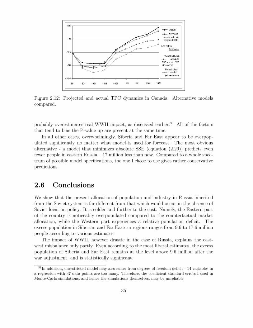
Figure 2.12: Projected and actual TPC dynamics in Canada. Alternative modelscompared.

probably overestimates real WWII impact, as discussed earlier.38 All of the factorsthat tend to bias the P-value up are present at the same time.

In all other cases, overwhelmingly, Siberia and Far East appear to be overpop-ulated significantly no matter what model is used for forecast. The most obviousalternative - a model that minimizes absolute SSE (equation (2.29)) predicts evenfewer people in eastern Russia – 17 million less than now. Compared to a whole spec-trum of possible model specifications, the one I chose to use gives rather conservativepredictions.

2.6 Conclusions

We show that the present allocation of population and industry in Russia inheritedfrom the Soviet system is far different from that which would occur in the absence ofSoviet location policy. It is colder and further to the east. Namely, the Eastern partof the country is noticeably overpopulated compared to the counterfactual marketallocation, while the Western part experiences a relative population deficit. Theexcess population in Siberian and Far Eastern regions ranges from 9.6 to 17.6 millionpeople according to various estimates.

The impact of WWII, however drastic in the case of Russia, explains the east-west misbalance only partly. Even according to the most liberal estimates, the excesspopulation of Siberia and Far East remains at the level above 9.6 million after thewar adjustment, and is statistically significant.

38In addition, unrestricted model may also suffer from degrees of freedom deficit - 14 variables ina regression with 37 data points are too many. Therefore, the coefficient standard errors I used inMonte-Carlo simulations, and hence the simulations themselves, may be unreliable.

35

Excess population in Siberia and Far East, ’000No correction Correction Correction Correction

Model for WWII for fertility for WWIIand fertility

Main resultMin. weighted 14,577 9,563 17,583 14,012SSE (<0.001) (0.005) (<0.001) (<0.001)

Alternative modelsMin. absolute 17,291 12,471 19,677 16,172SSE (<0.001) (<0.001) (<0.001) (<0.001)Unrestricted 13,030 6,260 15,914 10,882

(0.008) (0.131) (0.001) (0.028)P-values in parentheses

Table 2.2: Excess population in Siberia and Far East, according to alternative forecastmodels.

With the transition to market economy, as agents have the ability to freely respondto market stimuli, there might have been hope that the spatial inefficiency will correctitself eventually: people will migrate to more favorable places.

Indeed, starting from the early 1990s in post-communist Russia internal migrationdata show a pattern opposite to that of the Soviet times. People are leaving the North,Far East and Eastern Siberia. The European part of Russia, the Urals, as well assome industrial centers in Western Siberia (e.g. Omsk, Novosibirsk) see the migrationinflow.39 The rate of this migration, however, is slow.40 Heleniak’s (1999) estimateof the absolute decrease in population of Far North and Equivalent Territories (thesecorrespond roughly to Northern, Western and Eastern Siberia, and Far East in “usual”regional terminology, but do not include Novosibirsk, Omsk, Kemerovo, and Kurganoblasts) during the period from 1989 to 1998 is around 726,000 people41 (or about3.3% of population of these regions).

While this out-migration flow may seem significant in absolute magnitude, it isnowhere near the rate that it would take to bring the population distribution closerto what appear optimal in the foreseeable future.42 On average, Eastern regionsare overpopulated by a factor of 1.5. At the current rate, return to the optimaldistribution would take about 180 years. Thus, the costs of spatial inefficiency arelikely to be an extra burden for the new Russian state for years to come.

39Goskomstat, 1995. “Migratsia naselenia v Rossii.” (”Population Migration in Russia”)40Some territories are exceptions. For example, Magadan oblast and Chukotka republic lost 30-

40% of population during the transition years. It should be noted that these are the most remoteterritories with unbearable climate. Still, even at this rate of out-migration it would take 50-60 yearsminimum to revert to the counterfactual population levels in these territories.

41Data from Heleniak (1999), Table 4.42Heleniak also points out that some of the Western Siberian oblasts are popular designations for

the migrants from Siberian North and Far East. So, the total migration outflow from Siberia as awhole is actually lower than the numbers given.

36

Chapter 3

The Cost of the Cold

According to the results of the analysis presented in chapter 2, the spatial allocationof people and industry in Russia is highly distorted. If not for many decades ofcommunism, the spatial allocation of economic activity in Russia would have beendrastically different. At present the Siberian and Far Eastern regions are severelyoverpopulated. The simulated counterfactual market allocation is warmer: the actualpopulation-weighted aggregate January temperature index (TPC) is 1.5◦C lower thanthe counterfactual one. The next question is evident: since the allocation is found tobe inefficient, what are the consequences? Are the extra 1.5◦ of cold indeed costly forthe economy; and if yes, then what is the cost?

The chapter is organized as follows. Section 3.1 surveys the existing work onclimate-related costs of economic activity in relation to Russia’s circumstances. Thefollowing sections are devoted to estimating the costs of excess cold in Russia di-rectly. To calculate the cold-related cost of spatial inefficiency, I first investigate therelationship between temperature and various regional characteristics. I estimate thetemperature elasticities of energy consumption, health indicators, and productivity.Then, I use the estimated elasticities together with the measure of extra cold resultedfrom Soviet investment decisions — 1.5◦C TPC difference — to calculate the costin terms of present-day Russian GDP. Section 3.2 deals with additional energy con-sumption, section 3.3 evaluates the loss of productivity, section 3.4 explores healthissues with respect to climate, section 3.5 concludes.

3.1 The Role of Climate

The role of climate in economic performance is a widely debated question, mainly dueto the extensive literature on growth in tropical vs temperate countries. The well-known empirical regularity that tropical countries grow slower attracted conflictingexplanations. North (1990), Acemoglu, Johnson & Robinson (2002) point onto therole of institutions as the main factor in growth during the period after the industrialrevolution. Others (see for example Bloom & Sachs (1998)) offer an explanation thatfactors directly connected to country’s climate and geographical endowment, such as

37

disease transmission possibilities, being landlocked, land quality, etc, are responsiblefor the poor economic performance.1

The lack of consensus stems from the obvious puzzle in growth literature: eventhough the adverse effect of higher temperatures (or other factors highly correlatedwith it) is easily observed, it is not immediately clear what exact mechanisms arein play here. Generally, warmer climates provided more comfortable environmentfor human civilization in its early periods - in fact tropical areas used to be theonly places where the survival of human species was possible in prehistoric time.Intuitively, warmer climates should reduce cost of production and cost of living, andtherefore be conductive to economic growth ceteris paribus, not the opposite. Otherfactors that directly influence productivity must be at play, and it is not yet clear ifthey are really climate-related.

In contrast, the role of extremely cold climates is much less controversial. Beyondany doubt, cold climates increase production costs and the cost of living. Bothresidential housing and production facilities require extra energy for heating. Peoplerequire extra clothing. Constructing buildings and roads requires more materials.Agriculture in colder areas of the globe is limited or simply impossible. Transportationis more difficult. Cold is detrimental to people’s health. With modern technology,it is possible to partially mitigate the adverse effects of cold, i.e. adapt to it. Yetadaptation itself is costly.

Several studies have addressed the issue of cold-related economic costs before, andthe adverse effects of cold on productivity and quality of life are well documented. Hill& Gaddy (2003), chapter 3 discusses the work done to date on Canada and USA.2 Thegeneral conclusion is unambiguous: cold is costly. Abele (1986) finds that between 1and 2 % of labor productivity is lost when temperature drops by one ◦C in the rangebetween 0◦ and -20◦, more in lower temperatures. Herbert & Burton (1994) finds thatCanada spends about 1.6% of GDP annually to combat the effects of cold weather.Even in the relatively warm climate of USA, the 1◦C drop in temperature wouldhave resulted in extra costs amounted to 1.04 to 1.46% of GDP.3 Finally, Rosenthal,Gruenspecht & Moran (1995) found that in USA the extra costs of cooling broughtby Global Warming of 1◦C would be more than offset by lower costs of heating. Allthe studies suggest that for Russia the economic burden of cold could be just as, ifnot more severe.

While there is overwhelming evidence that operating in cold climates does indeedcarry a significant economic cost, the second motivating question remains: what isthe magnitude of costs in Russian case? The studies for US provide an informative

1The case of Russian regions and variation in their economic performance is particularly inter-esting in light of this debate. Russia represents a rare natural experiment where population wasdistributed (by the Soviet authorities, and in a manner largely exogenous to true economic incen-tives) across vast geographical space with diverse climatic conditions yet under the same set ofinstitutions.

2Including Abele (1986), Herbert & Burton (1994) and series of studies by the U.S. Departmentof Transportation. For summary, see Hill & Gaddy (2003).

3U.S. D.O.T. study, cited in Hill & Gaddy (2003).

38

benchmark, but cannot be directly applied to Russia. The differences in technologybetween Russia and US are profound - it is conceivably possible that adaptation tocold weather is significantly better in one of these economies: Russia (due to themassive Soviet investments) or, more likely, US (due to market economy incentives).Furthermore, what if the burden of cold is not simply proportional to temperaturedifferential, what if the cost of cold is non-linear? US January TPC is +4◦C vsRussian -12.9◦C. It is important to estimate the costs of cold specifically for Russianconditions.

Canadian studies of adaptation costs (Herbert & Burton (1994)) are more rele-vant for Russian case, as climatic conditions in Canada are closer to Russian ones.However, it answers a totally different question: it estimates the total costs of adap-tation, i.e. battling the cold weather. First, any adaptation to cold is partial: someof the adverse effects of cold cannot possibly be mitigated. Thus, Herbert & Burton(1994) provide only a lower-bound on total costs of cold. Second, my work concernsnot the total costs of cold per se, but rather the costs of extra cold in Russia, i.e.the climate-related costs of spatial misallocations by the Soviet system. Russia hasalways borne and will be bearing the costs of unfavorable location. Climate cannotbe changed; costs of poor climate in general cannot be prevented. Spatial misalloca-tions, however, can be corrected. How costly are these misallocations is the questiondirectly relevant for policy design.

3.2 Energy

This section studies energy consumption in Russia as a function of temperature. Insection 3.2.1 I look at the consumption of energy in producing sectors and calculatethe temperature elasticity of energy/labor ratio. In section 3.2.2 I estimate howdifferent would residential and commercial energy consumption for heating be in thecounterfactual allocation. Finally, section 3.2.3 combines the estimates for all sectorsand calculates the total extra energy costs.

For producing sectors, looking only at the energy/labor ratio does not reveal allof the extra energy costs due to cold. Cold may be detrimental to the productivity ofall the production factors - not only energy, but labor and capital as well. Therefore,it is possible (and likely) that to produce the same amount of output in a colderclimate one needs to have not only more energy, but more labor and more capital aswell. The estimates based on labor reflect the cost of cold only partially, and shouldbe treated as a lower bound on the true cost. Section 3.3, dedicated to productivity,addresses these questions further.

For residential and commercial sectors, due to data limitations I can only calculatechange in energy consumed for heating purposes. Most probably, extra heating costsare the most profound consequence of cold, but it is definitely not the only one. Itis possible that non-heating use if energy (lighting, cooking, etc) also increases withcold. As with the case of producing sectors, calculated energy cost in residential andcommercial sectors is just a lower bound on the true cost.

39

3.2.1 Energy use in producing sectors

The amount of energy used in production per unit of labor depends, in general, onproduction technology and, possibly, on the environment factors - climate. The goalof this exercise is to test if low temperatures indeed lead to higher industrial energyconsumption in Russia, and to quantify the effect, if any. I test the hypothesis onRussian regional data on aggregate consumption in producing sectors: agricultureand industry.4

Let the energy to labor requirement ratio in region i be dependent on temperaturein the following way:

lnEi

Li= α0 + αtt

◦i + εi (3.1)

where Ei is the amount of energy (electric, thermal or fossil fuel) used for productionin region i, Li - total industrial and agricultural employment in region i, t◦i - region’si average January temperature, εi - error term.

The error term εi reflects all regional idiosyncrasies pertaining to energy consump-tion. If the error term is orthogonal to temperature (random across geographicaldimension), the equation (3.1) can be estimated by OLS.

One of the factors that can affect a region’s energy consumption is industry struc-ture. A region specializing in energy-intensive industries is bound to use more energyin any climate. If the regional industrial structure in Russia follows a particular geo-graphic pattern, the εi are not independent of temperature, and we risk getting biasedestimates for the temperature elasticity. To account for interregional specialization,I include industry structure controls into the equation (3.1):

lnEi

Li= α0 +

m∑j=1

αjLij

Li+ αtt

◦i + εi (3.2)

where Lij - total employment by industry j in the region i (∑

j Lij + Agriculturei =Li). This way, the aggregate energy-to-labor ratio depends on industrial structure ofregional production and, additively, on temperature. The equation (3.2) is estimatedby OLS.

The data on electricity, thermal energy and fossil fuels used for production comesfrom the Goskomstat publications.5 Data on industrial and agricultural employmentcome from the Industrial Census of Soviet Union, 1989 and from Goskomstat.6 Tocreate industry structure controls (Lij), I grouped employment data by region (oblast)and by SIC code.

4In 1991 and 1992 the Russian State Committee for Statistics (Goskomstat) published regionaldata on energy “used for production of goods”. That includes the sectors producing material goods -industry and agriculture, and excludes commercial (services and government) and residential sectors.

5“Materialno-Technicheskoe Obespechenie v Rossiiskoi Federatsii”, 1992 and 1993.6“Regiony Rossii” (“Regions of Russia”), 1997.

40

The industry structure controls consist of employment shares in 2-digit SIC in-dustries and in some 4-digit SIC industries. To choose them, I first looked at data onthe energy-to-labor ratio for 2-digit and 4-digit SIC in order to pinpoint what 4-digitindustries are most likely to consume significantly more or significantly less energythat the 2-digit average. As a guide, I took the data for industry in US.7 If a 4-digitindustry had the energy-labor requirement ratio significantly higher or lower that 2-digit average, it was made into a separate series. For example, Primary Aluminum(SIC 3334), Pulp and Paper Mills (SIC 2611 and 2621) are among the “suspected”energy-intensive outliers and were separated from SIC33 and SIC26 groups. This way,I constructed 33 series of shares of 2-digit and 4-digit industries in total employment.(See Table C.5 for the list.)

The total of 33 industry series cannot be used at the same time in the regressionwith a sample size of 79 (regions). To ease the degrees of freedom deficit, The SICgroups that have roughly the same energy-labor ratios were combined. The groupsthat have energy-labor ratios close to the economy-wide average were dropped. Infinal regressions 10 to 12 separate control series were used.8

The Soviet Industrial Census gives data on the civilian enterprises only. A largeportion of economy (so called “VPK” - a Russian acronym for “Military-IndustrialComplex”) involved at least partially in the production of military goods is not in-cluded into the database. To make up for the omitted VPK employment, I use theestimates given by Horrigan (1992). The estimated VPK employment was added tothe regional civilian employment total (so that Li = Agricuturei + V PKi +

∑j Lij),

and VPK series was included into the set of industry controls.

Equation (3.2) models the dependence of temperature in additive way, thus essen-tially assumes that temperature affects all industries uniformly. Per equation (3.2)the extra energy required to operate in an environment one degree colder does notdepend on industrial structure. In reality, the “sensitivity” of the energy/labor re-quirement ratio to temperature may be different for different industries. However, totest for this in our environment, one we would need to include a set of interactionterms t◦i ∗ Lij

Li, which seems impossible with so many industry controls and only 79

regional observations in the data sample - degrees of freedom would be effectivelyexhausted.

The results are reported with and without the VPK-correction. Tables C.6-C.7shows the results for electricity consumption, Table C.8-C.9 - for thermal energy,Table C.10-C.11 - for fuels (see appendix C).

The estimated elasticities to temperature are highly significant and negative inboth years and for all types energy. The absolute values of the elasticity range from2.5% to 3.9% per degree Celsius. Including industry structure controls has little effecton either electricity or thermal energy elasticity estimates. For fuels, the temperature

7Per Energy Information Administration (EIA), in “Manufacturing Consumption of Energy1991”, on-line at <www.eia.doe.gov/emeu/mecs/mecs91/consumption/mecs1a.html>.

8As the regression results show, neither the coefficient of interest - the elasticity to temperature,nor its standard error changes significantly even when too many controls are added.

41

coefficient drops from 4.4% in 1991 (4.9% in 1992) to 2.5%(1991) and 3.4%(1992).The elasticity for electricity consumption is virtually the same (3.7-3.8% per ◦C)

for 1991 and 1992. For thermal energy and for fossil fuels the estimates differ sig-nificantly for 1991 and 1992. It is possible that the change in coefficients accuratelyreflects real structural changes in energy consumption patterns. In the end of 1991 -beginning of 1992 Russia went through price liberalization reform: the state controlof consumer prices was abandoned. A period of GDP fall and high inflation followed.Different temperature elasticities in 1991 and 1992 could reflect change in producers’behavior during these years - before and after reform. Of course alternatively, thediscrepancy in coefficients might be due to poor data quality.

Including VPK into the industrial totals and into controls does not seem to affectthe estimates. Marginally better R2 results with the VPK included in the model withindustrial controls, but not in the model without controls. The estimated coefficientsof VPK variable were not statistically different from that of other metal and machineryindustries (SIC 32-39), what prompted me to combine the series.

The elasticity estimates from 2.5% to almost 4% per degree translate into seriousenergy consumption differences in the Russian climate range. For example, most ofthe Western Siberian cities (Omsk, Tomsk, Novosibirsk to name a few), have Januarytemperatures 8 to 9 degrees C below that of Moscow. In the case of electricity, forexample, this difference translates into 27-30% higher per unit of labor requirementfor similar production processes. In order to finance this difference, about 10% ofall output (revenue) in the city of Omsk has to be spent!9 Of course, production inEastern Siberia requires even more of the extra energy. The extreme example is acity of Yakutsk, where production requires two times more electric energy per unit oflabor than in Moscow.

3.2.2 Residential energy consumption

The most significant consequence of cold are, probably, extra heating costs. Forthe residential and commercial structures the relationship between amount of energyrequired for heating and outside temperature may be adequately approximated by alinear function. The amount of energy required to heat a building with particularstructural characteristics over a period of time when the outside temperature varies isapproximately proportional to the number of degree-days below the building’s naturalbalance point.10 A balance point is a minimum outside temperature such that no

9Assuming the “extra” (compared to Moscow) energy consumption is all natural gas, sold for theaverage export price. If converted into oil at the export price, the “extra” energy would cost up to18% of output.

10From Rosenthal et al. (1995): “...In the case of direct combustion of fossil fuels the propor-tionality assumption is quite accurate... For electric heat pumps... the coefficient of performance isa (positive) function of the outside temperature...” Thus, energy requirement function of temper-ature is rather nonlinear with decreasing slope. Therefore, if we use linear approximation, we arerather understating the amount of energy used for heating in coldest Russian regions, and we areunderstating possible savings of this energy.

42

additional heating is required - the secondary inside sources of heat (people’s bodyheat, lighting fixtures or other appliances) and the building’s insulation are enough tokeep indoors warm.11 Given a balance point of b degrees Celsius, the yearly numberof degree-days in location i is calculated in the following way:

HDDi =365∑k=1

max(b − t◦ik, 0) (3.3)

To calculate the number of energy required for residential heating in a city (orregion), I assume that total energy used is proportional to the population of that city(region). In other words, I am assuming that there are no economies or diseconomiesof scale in residential heating.

In fact, economies of scale in heating are very probable. The well-known effectof “city warmth” is an excellent example. A large city generates a warm “pocket” -the average temperature in the center of the city is higher than in surrounding areas.This effect is easy to alleviate though, by using the actual temperature readings inthe city in question. The other effect is due to higher residential population density -per capita heating costs are inversely related to the number of floors in the buildingand directly to the amount of living space per capita. Thus more densely populatedareas tend to use less energy per capita.

On the other hand, the facts about Russian existing technology suggest some dis-economies of scale may be present. In most Russian urban areas buildings are heatedthrough a centralized system: the central boiler produces hot water and/or steam thatis distributed through the pipes to the residential and commercial buildings in thedistrict. The losses of thermal energy in transmission must be directly related to thelength of the communications, possibly making areas with more population less en-ergy efficient. It is difficult to say whether positive or negative effect of agglomerationon energy consumption actually prevails in Russian case.

With no economies/diseconomies of scale the total amount of energy for residentialheating in region i is:

ERi = C ∗ HDDi ∗ Populi (3.4)

where Populi is population of region i, C - proportionality coefficient. Then, if we as-sume that the structural characteristics of residential buildings in different regions arehomogeneous with respect to balance point, then the country-wide average residentialheating consumption per capita can be calculated as:

ER∑i Populi

= C ∗ HDDPC (3.5)

where HDDPC is a countrywide average number of heating degree-days per capita,calculated in the following way:

HDDPC =

∑i HDDi ∗ Populi∑

i Populi(3.6)

11A base point for residential housing used by US Energy Information Administration and byRosenthal et al. (1995) is 65 degrees Fahrenheit (18.3 degrees Celsius).

43

Simply put, under our assumptions the heating costs are proportional to the numberof heating degree-days per capita. The number of HDD’s per capita is a population-weighted average of degree-days in all the regions (equation (3.6)).12 To compare thecosts of residential heating in actual and counterfactual allocation one has to simplycompare the actual and counterfactual per capita HDD’s.

To construct an HDD per capita measure I use temperature data from NationalClimatic Data Center (CLIMVIS database).13 The CLIMVIS database provides dailyobservations of various climate indicators for about 8000 weather stations worldwide.I collected the mean temperature data for each day during 1994 to 2002 time periodfor 43 Russian stations. The stations chosen are located in or near former provincecapitals of Russian Empire that now lay within the borders of Russian Federation.Most of the cities are now oblast centers. I then calculated the average annual numberof heating degree-days according to equation (3.3).14 I used three base temperatures:10◦C, 5◦C and 18.3◦C.15

It is a practice in US Energy Information Administration to calculate heating andcooling degree-days from the base of 65F (18.3◦C). EIA divides all US territory intothe climate zones according to the number of 65F-base heating and cooling degree-days. In USA the places with more than 7000F heating degree-days (of 65F base),classified as “cold” climate zone, host 8.7% of total population. In Russia, 87% ofpopulation lives in “cold” climate zone, and the remaining 13% - in a second coldestzone, according to EIA classification.

The EIA standard of 18.3◦C heating base temperature was also used in the studyby Rosenthal et al. (1995). However in my opinion, lower base temperature has tobe adopted for the analysis of Russia. Accepting the 65F heating base for Russiawould imply that Moscow, for example, requires heating for 11 month a year, whichdoes not happen in reality. The normal heating period in Moscow is from 15th ofSeptember to 15th of May, and the target inside temperature must be at or above18 degrees Centigrade.16 For the analysis I am using the base temperature of 10◦C,which seems to be the most realistic in Russian case.

Table 3.1 presents the number of heating degree-days in selected Russian cities.First column shows the HDD for 10◦C base. For comparison purposes, numbers forthe different base temperatures are also given. The last column shows heating degree-days calculated in EIA standard (HDD for 65F/18.3◦C base), Fahrenheit equivalentis shown in parentheses.

The southern city of Makhachkala, the capital of Dagestan has the lowest num-ber of heating degree-days. By far coldest city is Yakutsk with 7549 HDD average.

12The way the HDD per capita measure is calculated is perfectly analogous to TPC - temperatureper capita index discussed in Mikhailova (2003).

13The database is on-line at <www.ncdc.noaa.gov/oa/climate/climatedata.html>.14All calculations are done in degrees Celsius.15Correspond to 50F, 40F and 65F.16The fact that Russia constructed housing stock with (on average, but not universally) a better

insulation than in the US suggests that some degree of adaptation to cold happened even under theSoviet system.

44

City HDD 10◦C HDD 5◦C HDD 18.3◦C (in F)Makhachkala 1076 339 2783 (5009)Moscow 2505 1417 4726 (8506)St. Petersburg 2510 1378 4856 (8740)Omsk 3829 2671 6078 (10942)Irkutsk 4295 3031 6718 (12095)Yakutsk 7549 6167 9998 (17996)Russian actualper capita average 2985 1883 5189Counterfactualper capita average 2817 1727 5010difference, % 5.7 8.3 3.5

Table 3.1: Heating degree-days for select cities and Russia as a whole.

Moscow and St. Petersburg have both near 2500 HDD annually. The number of HDDin Siberian cities ranges from about 3908 in Krasnoyarsk to about 4755 in Chita. Theaverage Siberian city has 60% more HDD, hence requires 60% more energy per resi-dent to provide heating, than Moscow!

To get the actual and counterfactual HDD’s per capita I plugged the actual andcounterfactual populations values into the equation (3.6). The actual number of(10◦C) HDD per capita is about 2985. The counterfactual HDD per capita is 2817- slightly more than Moscow average, and 5.7% less than actual. Thus, if marketforces allocated the population in Russia, the country as a whole would require atleast 5.7% less energy for residential heating.17

Furthermore, similar implications can be derived for commercial energy use. Com-mercial building stock hosts various non-manufacturing firms, mostly in the servicesector, and administrative functions. There is little regional variation in the share ofpeople employed in administrative and service sectors. Therefore, it is natural to ex-pect that in a counterfactual allocation the commercial sector, similarly to residential,would use about 5.7% less energy.

17An interesting topic for future work is the hypothesis that predominant structural characteristicsof Russian housing stock would have been different in a market economy environment. For such acold climate, insulation in average Russian housing units is way below adequate. (“...as much as800 kilowatt-hours per square meter per year are expended to heat multistory apartment blocks -roughly 10 times what is spent in developed countries.”- a quote from “Foreign Insulation Gets aWarm Welcome”, The St. Petersburg Times, January 10, 2003, By Robin Munro) The aggressivesubsidization of energy in the Soviet Union discouraged the use of more energy-efficient but moreexpensive materials and heating technologies. It is natural to expect that situation in a free marketenvironment would be drastically different. Although the goal of this paper is to isolate the effect ofspatial misallocations alone, one needs to bear in mind that the inherited Soviet distortions of othernature - structural, technological - also result in added burden to Russian economy. More researchis needed on how to mitigate the adverse effects of cold. Is it cheaper to insulate buildings, or tomove people away from cold places (or both)?

45

Energy savings Production sector energy Residential and commercialElectric Thermal Fossil fuels sector, energy for heating

“optimistic” version 5.55% 3% 3.75% 5.7%(1991 estimates)“pessimistic” version 5.7% 6% 5.25% 5.7%(1992 estimates)

Table 3.2: Savings of energy in counterfactual relative to actual allocation.

3.2.3 Cost

The next step is to calculate the cost of all the extra energy Russian economy usesbecause of its inefficient spatial allocation. First, the total amounts of “excess” energyused in production can be calculated using the estimated temperature elasticitiestogether with the difference between actual and counterfactual TPC’s:

∆E = αt ∗ ∆TPC (3.7)

The αt coefficients were estimated from a cross-sectional sample as described in section3.2.1. I calculate the cost for two sets of estimated elasticities: “optimistic” 1991values - 2% and 2.5% for thermal energy and fossil fuels, correspondingly, in 1991;and “pessimistic” 1992 values - 4% and 3.5%. Chapter 2 establishes the ∆TPC to be1.5◦C. Plugging this value together with the elasticities into the equation (3.7), getthe total percentage savings of energy in the counterfactual allocation (see Table 3.2).The residential and commercial energy consumption would have been 5.7% lower inthe counterfactual allocation, as established by the degree-days analysis, section 3.2.2.

The next step is to combine the estimated percentage savings with the exactamounts of each kind of energy consumed in either sector. To the best of my knowl-edge, only two sources exist for energy balances by sector: Goskomstat (partial data)and Asia Pacific Energy Council (APEC) energy balance reports (drawn on data sup-plied directly to APEC by Russian Fuel and Energy Ministry). 18,19 The data fromthese two sources sometimes disagree drastically. I used data on electricity consump-tion from Goskomstat, data on thermal energy industrial-residential breakdown fromOlkhovsky (2001), and data on fossil fuels sectoral breakdown from APEC EnergyBalance Tables. The diagram on Figure 3.1 summarizes the information on energysectors, what parts of total energy consumption did or did not go into the cost esti-mates.20 For production sector, I am using two values for each elasticity parameter -low (estimated from 1991 data) and high (from 1992).

18Goskomstat source: “Statistical Yearbook of Russia”, 2000.19APEC source: Asia Pacific Energy Research Centre, “APEC Energy Supply and Demand Out-

look, 2002”, Energy Balance Tables.20I calculate the cost given the limited data on energy consumption I could collect from available

sources. If and when more and better regional data becomes available, it would allow to fill in themissing estimates, conduct more thorough analysis, and to resolve the discrepancies between 1991

46

Figure 3.1: Energy sectors: consumption structure and counterfactual savings.

The shares of productive (industrial plus agricultural), residential, and commercialsectors in electricity consumption were calculated from Goskomstat data on electricenergy balance for years 1995-2001.21 The share of industrial sector in total energyconsumption has been steadily declining through these years, in my calculations Iused a simple average of yearly shares. The relative shares of other sectors remainedrelatively constant.

Residential and commercial share is somewhat more complicated to infer, sincethe data on consumption in these sectors are pooled together with transmission losses.To subtract the losses, I calculated the share of electricity losses in total consumptionin 2000 from Table 14.23 in “Statistical Yearbook of Russia”. According to Table14.23, transmission losses in electricity sector (35.0 million t.c.e) account for about12% of total electricity consumption (297.5 million t.c.e). So, I subtracted 12% oftotal from the average “other sectors...” consumption percentage. The remainder isthe 21% average share of residential and commercial sectors.

I assume that residential consumption of electricity (mostly for lighting and ap-pliances) does not change with temperature, thus the temperature elasticity is zero,which is possibly unreasonable. A small part of housing stock is heated with electric-

and 1992.21“Statistical Yearbook of Russia”, Table 14.25 on page 358 gives data on total consumption

together with consumption for industrial, agricultural, transportation sectors and “other sectorsand losses”. (The “other sectors and losses” category is a sum of consumption in residential andcommercial sectors plus total transmission losses in all sectors combined.)

47

Sector Consumption, Counterfactual Counterfactualmln t.c.e savings, % savings, mln t.c.e

Fossil fuels, residential 85.5 5.7 4.9Fossil fuels, production 149.6 3.8-5.3 5.7-7.9Fossil fuels, energy generation 408.6 3.8-5.3 15.5-21.7Electricity, residential 62.5 0 0Electricity, production 178.5 5.6-5.7 10.0-10.2Thermal energy, residential 92.3 5.7 5.3Thermal energy, production 113.7 3-6 3.4-6.8Total for the sectors above 1090.7 4.1-5.2 44.8-56.8

Table 3.3: Counterfactual “savings” of energy.

ity exclusively, and many households use electrical space heaters as a backup. Thus,the electricity savings are somewhat underestimated.

According to my estimates, fossil fuels used in the production process have atemperature elasticity of 2.5-3.5% per ◦C. I do not have regional data broken downby the type of use: how much fossil fuel was used as an input for (thermal andelectric) energy generation, and how much was used in final consumption for otherpurposed. Because of these data limitations, I have to assume that the consumptionof fossil fuels for all purposes has the same temperature elasticity. In productionsector, many firms use plant-size thermal stations that work on fuel, the generatedenergy is used both for heating and in technological processes, if required. Most ofthe fuel delivered to final consumers (households and firms) is used roughly in thesame way as in separate energy-generating facilities. Only a small part is used as araw material for chemical and allied industries (see Goskomstat energy balance, Table14.25 in “Statistical Yearbook of Russia”). Therefore, I do not believe the assumptionwould distort the results significantly.

To approximate the residential share of fossil fuels consumption, I took APECdata on residential and commercial consumption of three major components: naturalgas, oil and coal. Then, I calculated the share of it to the total consumption of gas,oil and coal. Production share is the remainder minus losses (from “Yearbook ofRussia”, Table 14.25) and minus the share of transportation sector.

For thermal energy, I first subtracted the share of losses (Goskomstat), then di-vided the remainder between residential/commercial and production sectors in pro-portion given by Olkhovsky (2001).

Table 3.3 combines the total energy consumption data (“Yearbook of Russia”,Table 14.25) and the inferred shares of each sector to give the absolute levels (intons of coal equivalent or t.c.e) of energy consumption in all sectors and calculate thecorresponding absolute savings.

The next step is to determine the cost of the 44.8 to 56.8 million t.c.e. of lostenergy. The price of one t.c.e. differs depending on the type of energy. I calculatethe cost in terms of natural gas, one of the cheapest of most common energy types.

An average representative heat content of 1000 cubic meters of natural gas is 36

48

GJ or 1.23 t.c.e. Thus, the 44.8-56.8 million t.c.e. of extra energy are equivalentto 36.4-46.2 billion cubic meters of natural gas. The average export price of naturalgas22 for year 2000 was 87.5 $US per 1000 cubic meters. The would-be savings ofenergy in 2000 translate into 3.1 to 4.1 billion dollars, or about 0.91 to 1.15% of 2000Russian nominal GDP23 of 349.4 billion $US.24

We must bear in mind that the energy costs are incurred on yearly basis. Thecost of lost investment opportunities accumulates over time. If the Russian economycould have grown 1 percentage point faster during the period of last 30 years (this iswhat would happen if there were no substantial increase in Siberian in-migration inthe 1970s, hence no sharp decrease in TPC), Russian GDP in 2000 would have beenabout 35% higher!25

I must add that many components of the total extra energy costs are still un-accounted for. In reality, electricity use by residential customers must have positivetemperature elasticity. Energy consumption by the transportation sector, for the pur-poses of this research is assumed to be independent on climate. In reality it mostly isincreasing with cold. More importantly, in Russia burning various kinds of fuel is themost common way of generating energy. Fuel has to be transported from the place ofproduction to consumers. If less people live in severe climates, not only less fuel wouldhave to be spent, but also less fuel would have to be transported over vast Russianspace. For many remote Russian regions transportation costs are comparable withthe cost of fuel itself.26 In counterfactual allocation, all those transportation costswould not be incurred. The cost of extra energy consumed is only a lower bound onthe true excess energy-related costs.

3.3 Productivity

In this section I investigate how total factor productivity interacts with cold. DoesTFP significantly decrease with extremely low temperatures? First, in subsection3.3.1 I examine how total gross regional product changes with temperature. Then, insection 3.3.2 I look at the construction industry, which is probably one of the sectorsthat exhibit the most interregional heterogeneity along the temperature dimension.

22Source: Goskomstat, “Statistical Yearbook of Russia”, 200023Source: Energy Information Administration, <www.eia.doe.gov/emeu/cabs/russia.html>.24Same calculations for more expensive crude oil (1.46 t.c.e. per ton, 175$US export price in 2000)

give counterfactual energy savings of 1.54 to 1.94% GDP.25Calculated under assumption of zero growth. Because of ruble devaluation during transition,

nominal GDP per capita growth (in currency exchange terms) in USSR/Russia from 1970 to 2000 isnear zero. If instead we assume average annual growth of 2.5% (typical for pre-transition decade),the result does not change significantly - lost GDP amounts to about 34%.

26The example of Kamchatka region is discussed in Hill & Gaddy (2003): for the region’s electricutility plants, the price of fuel transportation is about twice the price of fuel itself.

49

3.3.1 Aggregate Production

Suppose, the regional production function is of a Cobb-Douglas form and productionrequires two inputs: capital and labor:

Yi = Fi(Ki, Li) = AiKαi Lβ

i (3.8)

Where Ki is a capital stock in region i, Li is region i’s labor supply. Total FactorProductivity Ai varies across regions i and is a loglinear function of temperature(TEMPi), regional industrial structure, resource endowment and other controls (Xij),and the unobserved regional component εi:

ln Ai = Ao + A1TEMPi +∑

j

BjXij + εi (3.9)

Plugging (3.9) into (3.8) and taking logs, we obtain:

ln Yi = A0 + α lnKi + β ln Li + A1TEMPi +∑

j

BjXij + εi (3.10)

Equation (3.10) cannot be estimated directly by OLS because Li and Ki are notexogenously given, but are the variables of choice. When the production function asgiven by (3.10) is estimated with cross-sectional data, the factor with higher short-runmobility - labor - is usually instrumented for.

Contrary to common intuition, in Russia labor is less, not more mobile acrossregions than capital. Apparently, investment/disinvestments decisions produce morevariation in regional capital stock across time than interregional migration does forthe regional labor force. Regional labor supply is extremely stable, shockingly more sothan regional capital.27 A cross-sectional series of regional capital stock in 1994 andin 2000 are 92.6% correlated,28 while the series of regional labor force are correlatedat the 99.8% level. Thus, I am instrumenting capital with the regional populationpre-transition (1990).

As industry structure controls, I am using shares of the select industries in totalemployment. As appears, the most effective controls are the share of oil and gasextracting industry (SIC13) and the share of agricultural employment. Specializa-tion in oil and gas make regions appear more productive, dominance of agriculturenegatively affects the estimated TFP.

27This is not to say that the labor mobility is non-existent in Russia. On the level of individualfirms labor has been getting increasingly more mobile during the transition period. However, mostof labor movement is intersectoral but not interregional. The level of labor migration across regionsis still low.

28Note that capital stock is measured as the base (purchase) value of capital adjusted for depreci-ation at the official rate, and does not truly represent capital stock used for production. If a regionis economically successful and investment level is high, all new capital correctly shows up in data.If a region is in recession, capital is underutilized, and the measured capital stock is actually higherthan the utilized capital stock. Probably, capital is even more mobile across regions than it appearsto be.

50

Independent Dependent variable is the Log of GRPvariables in 2000Capital 0.95* 0.38 0.86* 0.34

(0.28) (0.26) (0.31) (0.26)Labor 0.23 0.70* 0.29 0.74*

(0.30) (0.26) (0.32) (0.28)Temperature -0.023* -0.013* -0.013 -0.011

(0.006) (0.006) (0.007) (0.006)Resource 0.25 0.09endowment index (0.13) (0.08)Industry structure no yes* no yes*controlsR2 0.85 0.92 0.86 0.95Heterosckedasticity-consistent standard errors arein parentheses. Number of observations is 72.* denotes significance at 95% level.

Table 3.4: Regional production function estimates (second stage).

As an alternative (or additional) control variable I also used the regional resourceendowment index compiled by World Bank. The index value varies from zero forMoscow city to 2.2 for oil-rich Tuymen’.

The results are shown in Table 3.4.29 Evidently, the temperature coefficient isnot of the expected sign, and statistically significant. Low temperatures seem not tohurt production, but help it! The coefficient loses some of the significance if industrystructure controls are included, but is far from being positive, as our hypothesis wouldpredict.

The reason for the negative sign of temperature may be interregional incomeand price level differences. Cold regions tend to have higher nominal incomes andhigher cost of living. Higher local nominal incomes would imply higher prices fornon-traded goods in colder regions. Even in the case of traded goods, the substantialtransportation costs (in a large country like Russia regions are dispersed spatially)would insure that some degree of interregional price differential would exist. Moreover,Gluschenko (2002) shows that the law of one price does not hold for Russian regionseven when transportation costs are accounted for. Thus, price-income patterns inRussia exhibit a Balassa-Samuelson-type effect: richer regions have higher prices, evenfor traded goods. Higher wages in resource-extracting industries lead to higher pricesfor non-traded goods and services and, as a consequence pump up the prices for tradedgoods through service component in final price. Concurrently, lower temperatures areassociated with higher prices. Thus, even if a firm in a cold region is producing thesame amount of real output as a comparable firm in a warm region, chances are

29The estimated shares of labor and capital are very sensitive to specification. Including industrycontrols changes the results drastically. This is yet one more indication that production functionsare highly heterogeneous across industries. Additional work is needed to estimate the productionfunction, perhaps using data disaggregated on industry level.

51

Figure 3.2: Gross regional product, prices and temperature.

that the “cold” firm would record higher output in monetary terms. Since laboris measured in real terms - number of people employed - the estimates of TFP inhigh-price regions are inflated.30

To overcome this problem would require data on real regional output, i.e. we needto deflate the nominal output by a regional producer price index. The only cross-sectional price indices available from Goskomstat are the cost of 19- and 25-goodconsumer baskets31 and the local subsistence minimum.

The results with the dependent variable - gross regional product - deflated by thesubsistence minimum are in Table 3.5.

With deflated GRP data, the temperature elasticity estimates have increased.However, it is yet unclear whether the result is robust to the choice of deflator. Usingthe price of either consumer basket as a deflator yields virtually the same results, sincethey are highly correlated with subsistence minimum. Both indices are based on mostnecessary consumer items and are poor proxy for producer price index. It is possiblethat the producer prices vary less (or more) across regions than subsistence minimumand consumer prices, thus the temperature elasticity in Table 3.5 is overestimated (orunderestimated).

Further research of the relationship between productivity and climate is needed.One of the possible directions is to estimate the production function at the level of

30It is not clear if price differentials among regions affect capital valuation in Russia. Theoretically,if value of capital is dependent on local price level, the coefficients α and β would also be biased.However, I know not of any evidence that would link capital valuation to consumer price index, andcannot conclusively argue one way or the other.

31The consumer baskets represents most necessary products, mostly food.

52

Independent Dependent variable is the Log ofvariables GRP/Subsistance in 2000Capital 0.22 -0.04 0.14* -0.08

(1.33) (0.20) (0.25) (0.21)Labor 1.03* 1.25* 1.08* 1.29*

(0.23) (0.20) (0.25) (0.22)Temperature -0.008 -0.004 -0.0005 -0.0005

(0.004) (0.006) (0.005) (0.004)Resource 0.20* 0.09*endowment index (0.07) (0.06)Industry structure no yes* no yes*controlsR2 0.91 0.94 0.92 0.95Heterosckedasticity-consistent standard errors arein parentheses. Number of observations is 72.* denotes significance at 95% level.

Table 3.5: Regional production function estimates, GRP deflated by subsistence min-imum index (second stage).

industry. The production process is more homogeneous inside a particular industrythan on the level of aggregate production, thus we should be able to estimate thecoefficients of labor and capital (β and α), and the TFP better. Moreover, the pro-ducer prices inside the same industry are more comparable across regions, especiallyfor traded goods. Therefore, even without using the regional price level deflator, wecan analyze the data for output in an industry that produces traded goods yet stillestimate the temperature elasticity with little or no bias.

I would expect the temperature elasticity of TFP to be positive and highest in theindustries where production process is not climate controlled, such as construction,forestry and logging. In the industries where the production process is conductedindoors, I would expect little or no effect of climate on the productivity itself, butthe higher costs of extra energy consumption.

3.3.2 Construction

This subsection analyzes the effect of climate on the productivity of the constructionindustry. There are three reasons for construction costs to be higher in cold cli-mates. First, the material requirements must be higher in cold climates: comparablestructures, for example residential housing, must provide higher degree of insulation.Second, productivity of machinery and labor must be negatively affected by cold.32

Finally, equipment, buildings and roads deteriorate faster in cold climates and requiremore maintenance and have to be replaced more often.

32See for example, the table of the cost thresholds for standard equipment in Siberia, by Mote,cited in Hill & Gaddy (2003) and in Gaddy & Ickes (2001).

53

Dependent ROADS BUILDINGS Number R2

variable of obs.Construction 2.19 1.29 74 0.77output, mln rub (1.48) (0.08)Heterosckedasticity-consistent standard errors are in parentheses.

Table 3.6: Relative prices of construction output.

The data available to date on construction in Russian regions allow to measureonly one of the costs: the loss of productivity. Goskomstat33 publishes both industry-specific data on labor, capital and data on production in real-terms. It tells exactlyhow many cubic meters of buildings were constructed, how many kilometers of roadsand communications were built. The availability of real-terms data is welcome becauseof the difficulty with calculating the interregional price level differences in Russiaas discussed in section 3.3.1. The temperature elasticity estimates based upon thenominal output data are bound to be biased downward.

Using data from Goskomstat34. I estimate the construction industry productionfunction and test whether temperature has a significant effect on total factor pro-ductivity. As in section 3.3.1, consider a Cobb-Douglas production function given by(3.8) with Total Factor Productivity being a function of temperature. The estimatedequation is (3.10), where Yi is the real output in construction industry in region i, Ki

and Li are capital and labor employed in construction.Yi is supposed to represent the total amount of real output in construction. How-

ever, construction output is not fully homogeneous. Goskomstat gives separate dataon length of roads and volume of buildings constructed.35 Different varieties of con-struction product have to be aggregated into a composite measure.

How should we aggregate output from different kinds of construction projects? Isum up the data on buildings and on roads weighted by their relative prices. Pricesare estimated out of the equation (3.11).

I run a regression of total construction output (monetary value) on the physicalvolumes of buildings and roads construction. The ratio of the estimated coefficientsrepresent the relative price ratio sought after.

PiYi = ProadsROADSi + PbuildBUILDINGSi + δi (3.11)

Where PiYi - monetary value of construction output in region i. The most likelyoutliers - Moscow, Moscow region, St. Petersburg, Tyumen’ region were droppedfrom the sample. The results are presented in Table 3.6.

33“Stroitel’stvo v Rossii”(“Construction in Russia”), 2000.34“Construction in Russia”, 2000.35Data on length of water, sewer and other types of communications constructed are also given,

but their average monetary share in output is relatively small and the amounts are highly correlatedwith volume of buildings construction. Because of its high correlation with buildings constructionvolume, omitting this category of output would not change the results. I did not use these data.

54

Dependent Const Log of Number R2

variable Labor 1990 of obs.Log of Construction -4.957 1.242 72 0.91labor, 1999 (0.308) (0.045)Heteroskedasticity-consistent standard errors are in parentheses.

Table 3.7: Construction industry production function IV estimation. First stage.

Under the assumption that relative prices reflect relative costs of different con-struction products, the aggregate index of real output Yi (to the multiplicative con-stant) is calculated as a weighted sum of real outputs in two sectors:

CYi = ProadsROADSi + PbuildBUILDINGSi (3.12)

Now using the constructed weighted index of real construction output CYi we canestimate the equation (3.10).

As with the case of total production, the equation (3.10) cannot be estimateddirectly by OLS because Li and Ki are endogenous. In the case of construction,however, it is labor that has to be instrumented for. Even though interregional labormigration in Russia is almost nonexistent, inside the region labor is sufficiently mobilebetween sectors and industries. Labor employed in a particular industry is capableof short-run adjustment and surely endogenous, especially in construction industrywhere people are often hired for specific projects, on on-demand basis.

As an instrument for construction labor I take the regional data on total laborforce in 1990. While the total number of employed is highly correlated with employedin construction (even though the series are separated by 9 years), it is likely to beorthogonal to the present-day region-specific productivity shocks, because spatialallocation of labor force in 1990 is a legacy of Soviet planning, not a response tomarket conditions. The results of the first stage IV regression are in Table 3.7.

Table 3.8 presents the results of the second-stage IV estimates, along with an OLSregression for comparison. Magadan and Yakutia regions, both bitterly cold (but notthe only bitterly cold regions) proved to be outliers. When these two regions aredropped from the sample, the estimated temperature elasticity drops from -1.6% per◦C to -2.3% per ◦C. In both cases, the temperature coefficient is strictly significantstatistically.

To check if the estimated temperature coefficient is robust to the weighting usedto construct the real output index, I also estimate IV regressions with the dependentvariable being only roads constructed and only buildings constructed. The results arein Table 3.9.

As the results show, the temperature coefficient remains virtually unchanged ifwe choose to measure construction output taking into account only buildings, oronly roads. Thus, the dependence on temperature is not induced by the particularweighting method I used.

55

Dependent variable is Log of real construction output weighted indexIndependent variables OLS IV OLS IVConstant 4.765 5.285 4.579 5.172

(0.345) (0.291) (0.384) (0.319)Log of Capital -0.055 0.166 -0.053 0.213

(0.076) (0.063) (0.078) (0.074)Log of Labor 0.953 0.770 0.981 0.767

(0.097) (0.072) (0.109) (0.086)Temperature 0.022 0.023 0.014 0.016

(0.010) (0.009) (0.011) (0.011)Magadan and Yakutia included no no yes yesNumber of observations 76 70 78 72R2 0.88 0.82 0.84 0.77Heteroskedasticity-consistent standard errors are in parentheses.

Table 3.8: Construction industry production function IV estimation. Second stage.

Dependent variableLog of building Log of real output Log of roads

Independent variables space , m3 weighted index length, kmConstant 4.859 5.285 2.349

(0.313) (0.291) (0.513)Log of Capital 0.154 0.166 0.179

(0.070) (0.063) (0.172)Log of Labor 0.795 0.770 0.563

(0.078) (0.072) (0.176)Temperature 0.022 0.023 0.024

(0.010) (0.009) (0.020)Number of obs. 70 70 66R2 0.81 0.82 0.31Heteroskedasticity-consistent standard errors are in parentheses.

Table 3.9: Production function estimates. Test of the robustness to the weighting.

56

To summarize, the findings do support the hypothesis that cold harms construc-tion productivity. 36 The estimated productivity loss is about 2.3% per degree Centi-grade. An average Siberian city requires 23-25% more labor and capital resourcesthen Moscow to complete a comparable task. The inherited spatial inefficiency, theextra -1.5 ◦C of TPC according to chapter 2, costs the Russian construction indus-try 3.4% of total output country-wide in productivity loss alone. Value added inthe construction industry is responsible for about 6.4% of Russian GDP, hence lostproductivity in the construction industry translates into about 0.22% GDP loss, duesimply to lower efficiency of work. Recall that productivity loss is only a part of totalcosts - as the costs of extra materials and costs of premature depreciation of buildingsand communications are not accounted for.

3.4 Health

I now turn to the input of temperature on health. I begin with analyzing the effectof temperature on people’s health. First, I estimate the elasticity of health indica-tors to temperature (I look at regional mortality and morbidity). Then, I use thecounterfactual-actual TPC difference of 1.5◦C to predict the aggregate health indica-tors in the counterfactual allocation.

3.4.1 Mortality and morbidity

The nature of mortality or morbidity data is probabilistic: aggregate per capitameasures are confined between zero and one. A non-linear model of probability hasto be employed. I use a logit setup. Assume the probability of an event (either illnessor death) for a person i in region j takes the form:

Pij = Prob{xjβ + δj + εi > 0} (3.13)

36Rosen (1979), chapter 6 provides evidence on the effect Winter House Building Initiative inCanada - a program subsidizing construction of housing during December-March period. A moderatesubsidy provided by WHBI was enough to significantly shift the seasonal pattern of constructiontoward winter months, which seem to suggest that added costs of building in winter are relativelysmall, contrary to my own findings. However, three factors must be considered comparing CanadianWHBI experience with Russian evidence. First, as Rosen points out, the main effect of a subsidywas to effectively decrease the downpayment requirement for winter-built housing, hence significantlyincrease demand. The increased demand might have brought an increase in producer surplus abovethe nominal value of the subsidy. Second, winter weather in the most densely populated areasin Canada - southern Ontario and Quebec - is way milder than in Russian Siberia and Far East.Perhaps, the loss of productivity due to cold is non-linear, accelerating as temperatures drop. Thus,my estimated elasticity is relevant in Russian temperature range, but not in Canadian. Finally, evenif the effect of temperature itself on productivity were indeed small, my results would imply thatsome other factors correlated with temperature affect construction productivity. However, this doesnot change the main conclusion of the paper: Soviet spatial misallocations result in productivityloss, be it due to cold or some unobserved regional heterogeneity.

57

where xj - observable characteristics of region j, δj - unobserved region-specific shock,εi - person-specific shock, β - parameter vector. Assume there are infinite number ofpeople in each region and that εi are Weibull-distributed. Integrating over individualsget the expression for aggregate event probability in region j:

Pj =exjβ+δj

1 + exjβ+δj(3.14)

Substituting the observed mortality or morbidity rates Sj instead of theoretical prob-ability Pj and applying the logit transformation, get:

lnSj

1 − Sj

= xjβ + δj (3.15)

Assuming the region-specific shocks are independent and Normal-distributed, theequation (3.15) can be estimated by OLS.

The set of control variables xj includes temperature and various social and eco-nomic characteristics, such as average income, various proxies for the level of devel-opment of regional infrastructure and health services. I use regional income levels,number of doctors per capita and (for adult mortality) amount of alcohol productssold per capita. Some, if not all, of these variables may be endogenous to healthindicators. For example, number of doctors in the region may have direct positiveeffect on health, or/and at the same time reflect the reverse causality: a region withpoor health indicators may choose to attract more doctors (with or without federalhelp). High levels of alcohol consumption may be associated with (or even causedby) low overall quality of life, health notwithstanding. However, since my interest iswith the temperature coefficient, I will not address the issues of possible endogeneityin other control variables. My purpose in using these controls is only to make surethat the temperature coefficient is robust to specification.

The results for aggregate (not age-standardized) morbidity and mortality are givenin Tables 3.10 and 3.11. Note that mortality seems to be increasing with temperature,contrary to common sense. The temperature elasticity of morbidity has the expectednegative sign. To explain the results, note that these mortality and morbidity dataare not age-standardized.

The real reason why temperature may seem either harmful or irrelevant lies inRussian migration patterns. Higher wages in Siberia and the Far East traditionallyhave been attracting young healthy people. Young migrants “bring good health”into Siberia. In contrast, retirees have always been trying to relocate back to theEuropean part of country, especially to the warm southern regions of North Caucasus.Poor health of long-term Siberian residents was dissipated over the whole country.Analogous to “Florida effect”, such self-selection of people over climate zones biasesthe temperature coefficient up. Young people are less likely to get sick than elderly,and surely they are much less likely to die. Because of the life-cycle migration patternsthe elasticities for both aggregate mortality and morbidity are likely to be biased

58

Dependent variable (S) is average morbidity rate 1992-2000Model Logistic (ln( S

1−S )) Linear (ln(S))Temperature (◦C) -0.025 -0.017 -0.017 -0.009 -0.006 -0.006

(0.01) (0.08) (0.08) (0.02) (0.03) (0.12)Doctors per 0.000 0.001capita, average (0.92) (0.77)Alcohol sales 0.093 0.093 0.040 0.040per capita, ’91 (l) (0.04) (0.04) (0.02) (0.02)Income, ’90 (rub) 0.002 0.003 0.001 0.001

(0.01) (0.02) (0.01) (0.03)Elasticity to t◦ %

◦C -0.8 -0.6 -0.6 -0.9 -0.6 -0.6Number of obs 79 73 73 79 73 73R2 0.11 0.26 0.27 0.11 0.28 0.28Heteroskedasticity-consistent P-values are in parentheses.

Table 3.10: Aggregate morbidity rate as a function of temperature. Robustness tospecification.

Dependent variable (S) is average mortality rate 1992-2000Model Logistic (ln( S

1−S )) Linear (ln(S))Temperature (◦C) 0.009 0.016 0.016 0.010 0.004 0.004

(0.00) (0.01) (0.00) (0.00) (0.00) (0.19)Doctors per -0.001 -0.001capita, average (0.80) (0.81)Alcohol sales 0.070 0.070 0.069 0.069per capita, ’91 (l) (0.00) (0.00) (0.00) (0.00)Income, ’90 (rub) -0.002 -0.002 -0.002 -0.002

(0.00) (0.00) (0.00) (0.00)Elasticity to t◦ ( %

◦C ) +0.9 +0.4 +0.4 +1.0 +0.4 +0.4Number of obs 78 72 72 78 72 72R2 0.11 0.13 0.23 0.10 0.13 0.45Heteroskedasticity-consistent P-values are in parentheses.

Table 3.11: Aggregate mortality rate as a function of temperature. Robustness tospecification.

59

Dep. var. is Independent variablesstandardized Temp. Doctors Alcohol sales Income Numbermortality rate ( %

◦C ) per capita p/capita, ’91 ’95 (th rub) of obs R2

’97-’98 -0.57 0.000 0.027 0.002 77 0.40average total (0.00) (0.89) (0.00) (0.97)’97-’98 -0.54 -0.001 0.038 -0.072 77 0.39average male (0.00) (0.73) (0.00) (0.24)’97-’98 -0.63 0.000 0.019 0.044 77 0.41average female (0.00) (0.83) (0.03) (0.53)Dependent variable is logit-transformed. Heteroskedasticity-consistent P-values arein parentheses.

Table 3.12: Standardized mortality rate as a function of temperature.

upward. Looking at the age-standardized levels of mortality and morbidity insteadof the simple aggregate levels may cure the problem partially.

Data on standardized mortality based on mortality and age data collected byGoskomstat, are published in bimonthly journal of Russian Health Ministry. Un-fortunately, to the best of my knowledge, there are no standardized morbidity ratesby region published in Goskomstat or other official sources. Therefore, in furtheranalysis I concentrate on mortality only.

Indeed, if instead of looking at the simple aggregate mortality we look at age-standardized values, the temperature coefficient changes to negative and statisticallysignificant.

Standardization by age removes the inter-generational selection bias, but the biasdue to self-selection inside the same age group is still present. Of the young people,the healthier ones are more likely to migrate to colder regions. The less healthypeople of any age are also more likely to leave the colder regions for places morecomfortable. Note that if selective migration is more pronounced among men, womenwould have higher estimated elasticity to temperature, which is not inconsistent withthe findings.37 The temperature elasticity for female mortality is higher consistentlyover the years. This pattern is highly suggestive of the hypothesis that at least inRussia mostly men choose the place to work, and women follow.

Since self-selection bias is present in the estimates, it is fair to treat the estimatedtemperature elasticity as a upper-bound (lower-bound in absolute value) on trueelasticity value. However, given low overall levels of labor migration in Russia theselection for most of regions is likely small, possibly negligible (Tuymen’ might be theonly exception).38

37The elasticity estimates are not statistically different for men and women, each having a standarderror of 0.17 % per ◦C.

38One might argue that the elevated levels of mortality in colder regions are not the consequenceof cold per se, but instead owe to other factors, such as remoteness, luck of infrastructure, poorerqualifications of medical personnel and overall lower standard of living, since all these factors arehighly correlated with (or sometimes endogenous to) temperature in Russian case. The argument

60

Looking at infant mortality can shed some light on the size of the remainingselection bias. Infants are the only age group for which climate-selection does not yetcome to play (parents can decide to move to more comfortable environment, or decideagainst moving to cold place if their child’s poor health can be affected by climate,but moving takes time).39

The estimated elasticity of infant mortality to temperature is indeed slightly higherin absolute value than the elasticity of (even standardized) mortality rate of adults,and this is true consistently over time.40 On one hand, a higher elasticity might becaused by physiological differences: maybe cold climates are more harmful for infantsthan for adults.41 On the other hand, if cold is equally bad for children and adults,then the elasticity of mortality for infants is representative of all age groups and cleanof self-selection bias. Yet in both cases, to the hypothesis that “men choose, womenfollow” we may now add “and children pay the price”.

The selection bias in adult data cannot be either proved or fully corrected forusing only aggregate regional information. More research is needed on the influenceof climate on health, if and when a significantly large and regionally representativesample of individual-level data is available.

It is also important to conduct separate estimations for rural and urban infantmortality, using the data available for recent years. The purpose is to investigate iftemperature proves to be a more significant factor for either urban or rural infantmortality. The results are rather uninformative. Splitting the data turns both coeffi-cients insignificant. For rural data, income suddenly appears to be main explanatoryfactor, and the urban regression is generally poor. Vassin & Costello (1997) foundthat the Russian mortality patterns, just as the overall state of the economy, societyand health, differ much more between urban and rural areas than between regions.There exist unobserved heterogeneity between urban and rural Russia. Perhaps, bet-ter control variables are needed: temperature, health infrastructure data aggregatedseparately over urban and rural areas might be more informative. Even geographiccenters of urban and rural population of the same region might be different, and hencehave different average temperature (TPC). More careful treatment of urban-rural dif-ferences is needed in order to satisfactory investigate the role of temperature.

3.4.2 What is the cost of the excess mortality?

The next logical question is: what are the economic consequences of the excess mortal-ity brought about by the Soviet misallocations? We can consider two estimates. Oneis the estimate of the direct cost of mortality: the reduction in economic growth, loss

has a lot of merit, it does not however change the main conclusion: whether because of cold orbecause of distance or other factors, overpopulation of the East is costly to Russian economy.

39Infants’ health could be subject to some degree of selection bias: if parents are healthier onaverage, so are the children; but hopefully this effect is relatively negligible.

40Though not statistically different in any given year.41As an obvious example, respiratory diseases - dangerous for infants and elderly - are spreading

faster in cold climates, simply because people spend more time together indoors.

61

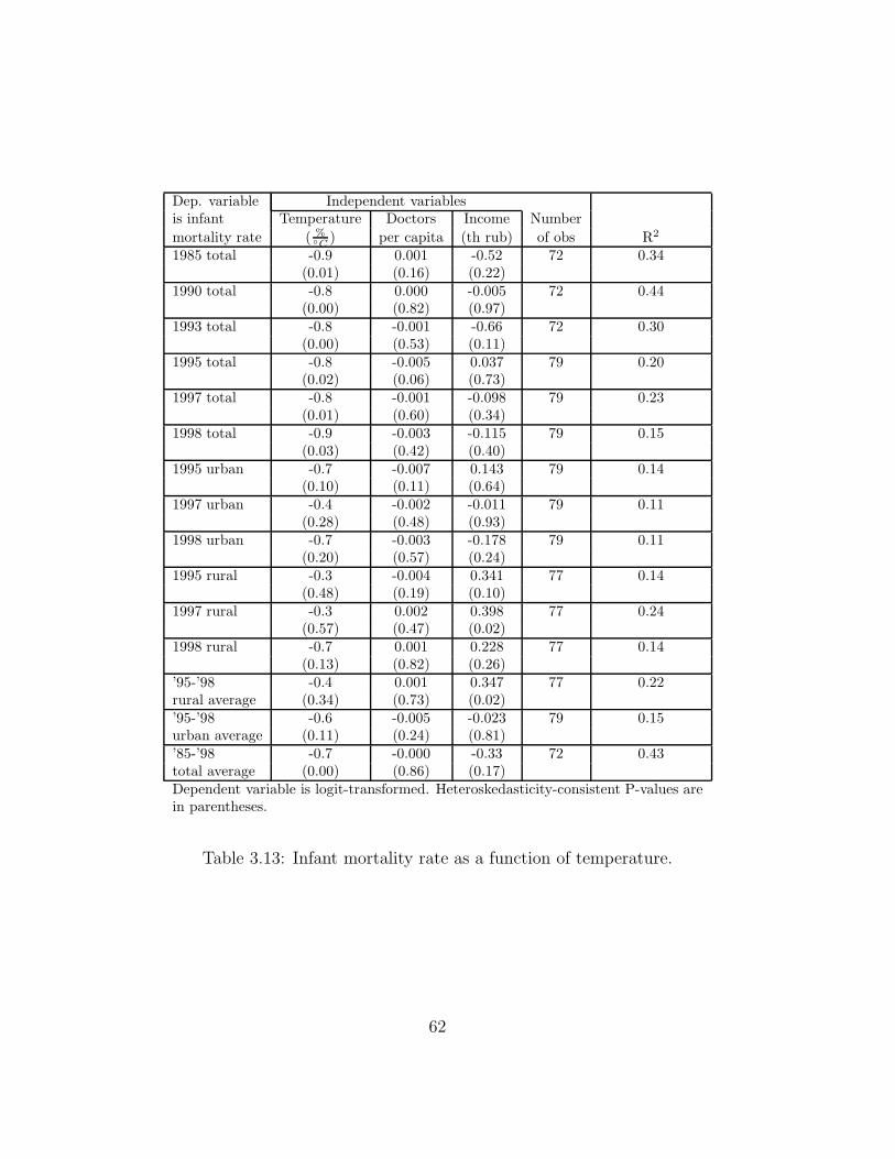
Dep. variable Independent variablesis infant Temperature Doctors Income Numbermortality rate ( %

◦C ) per capita (th rub) of obs R2

1985 total -0.9 0.001 -0.52 72 0.34(0.01) (0.16) (0.22)

1990 total -0.8 0.000 -0.005 72 0.44(0.00) (0.82) (0.97)

1993 total -0.8 -0.001 -0.66 72 0.30(0.00) (0.53) (0.11)

1995 total -0.8 -0.005 0.037 79 0.20(0.02) (0.06) (0.73)

1997 total -0.8 -0.001 -0.098 79 0.23(0.01) (0.60) (0.34)

1998 total -0.9 -0.003 -0.115 79 0.15(0.03) (0.42) (0.40)

1995 urban -0.7 -0.007 0.143 79 0.14(0.10) (0.11) (0.64)

1997 urban -0.4 -0.002 -0.011 79 0.11(0.28) (0.48) (0.93)

1998 urban -0.7 -0.003 -0.178 79 0.11(0.20) (0.57) (0.24)

1995 rural -0.3 -0.004 0.341 77 0.14(0.48) (0.19) (0.10)

1997 rural -0.3 0.002 0.398 77 0.24(0.57) (0.47) (0.02)

1998 rural -0.7 0.001 0.228 77 0.14(0.13) (0.82) (0.26)

’95-’98 -0.4 0.001 0.347 77 0.22rural average (0.34) (0.73) (0.02)’95-’98 -0.6 -0.005 -0.023 79 0.15urban average (0.11) (0.24) (0.81)’85-’98 -0.7 -0.000 -0.33 72 0.43total average (0.00) (0.86) (0.17)Dependent variable is logit-transformed. Heteroskedasticity-consistent P-values arein parentheses.

Table 3.13: Infant mortality rate as a function of temperature.

62

of output and utility because of shorter life expectancy. If we obtain an estimate forthe economic value of life in Russia, we can calculate the aggregate economic impactof decreased life expectancy based on actual-counterfactual mortality differential.

The other estimate is the amount of money it would take to mitigate the cost ofextra cold: invest in and develop medical infrastructure enough to bring mortality tothe counterfactual levels. In a competitive decentralized economy (or with benevo-lent social planner), we can assume that if a reduction in mortality were economicallyefficient, it would have happened. It is not necessarily so in the Soviet system. There-fore, the opportunity cost of excess mortality in Russia is really the lower of the twoestimates mentioned above.

The studies of growth in a cross-country setting so far show that higher mortalityis weakly associated with slower growth. Barro & Sala-i-Martin (1995) present sup-porting evidence but only for the countries with per capita GDP of somewhat below$1000. For richer countries (Russia included) no relationship between mortality andgrowth was observed. However it is still unclear where real causality lies. Is it lowermortality that causes higher growth? Or does economic success lead to better healthsituation? The issue is far from being conclusively resolved, and any extrapolationsof the international results to the Russian case should be taken with the grain ofsalt.42 The consequences of higher mortality for Russia’s economic performance arean important direction for future research. But even in most modest scenario, ifpure economic costs of excess mortality in Russia are close to zero, the social cost ofdecreased life expectancy is hardly a factor to ignore.

3.5 Conclusions

The purpose of this paper was to determine how costly is the cold for Russia. Myanswer is: very. Lower temperatures lead to higher energy consumption and highermortality. More research is needed to investigate the effect on productivity of varioussectors of the economy. If the construction industry is at all representative, it isreasonable to expect negative effect on productivity in many if not all sectors.

The legacy of the Soviet system leaves Russia 1.5◦C colder in per capita terms. Inthe most modest of estimates, this difference in TPC costs not less than 1% of GDPin extra energy costs, and 0.2% of GDP in lost productivity in construction sectoralone annually. If all manufacturing industries had the same temperature elasticityof TFP as construction, loss of another 1.3% of GDP yearly could be attributed tocold. Additional 0.85% of aggregate mortality are also a direct consequence of Sovietspatial policy. These are annual costs, but compounded over last 30 years of theSoviet era - a time when the spatial evolution of Russian economy took a sharpestdetour from the optimal trajectory - lead to a GDP loss in excess of 35% (or 97% in

42Intuition suggests, however, that higher mortality must indeed have adverse effect on GDPceteris paribus. Higher mortality must be associated with higher morbidity. Higher morbidity ratenecessarily leads to lower productivity of labor and reduces the labor force.

63

worst case scenario). Every person in Russia gave up at least one fourth (or maybea half) of his income for Siberian development!

Two directions for future research are evident. First, the analysis could be furtherimproved and expanded, especially with respect to productivity. The elasticity of TFPto temperature in different sectors or industries could be further investigated with theappropriate data on regional output, capital and labor disaggregated by industry. Theanalysis of energy consumption could benefit from better and more complete data. Inparticular, due to data constraints residential electricity consumption was assumedto have zero temperature elasticity. In reality, in Russia (where air conditioning ismuch less common than electrical space heating) it is probably negative. If we hadthe proper data, it is likely that the estimates would add to the total assessment ofthe costs of cold.

A second direction for future research deals with designing the appropriate policy.The cold is costly, and the extra cold due to the Soviet misallocations is an extraunnecessary burden, but what could be done about it? Given the spatial structureof Russian economy formed by the Soviet system, more research is needed on theoptimal policies that would help to restore or improve spatial efficiency. Is it betterto adapt to cold or to move people to warmer places?

64

Appendix A

Details of dataset construction

A.1 Dependent variables: population and manu-

facturing employment

Russia

The population and manufacturing employment data for Russia (POPULt and INDt)for the pre-revolutionary period were taken from the “Yearbook of Russia, 1910.” Thedata on population by administrative units are quite accurate and extensive.

For manufacturing employment data I used two alternative sources. First, I usethe reports of the 1908 census of industry that give the number of people employed inmanufacturing enterprises (5 or more employees). Secondly, I the report on peoples’occupations by province.1 The number of people reported to be in manufacturingoccupations (group VII occupations: manufacturing, mining and crafts) is normallyhigher than number of employed counted by census of industry, because small andfamily establishments (less than 5 people) were not covered by industrial census. Thechoice of data series did not prove important, as the final results turned out to differonly by fractions of 1%.

There were 98 administrative units – “gubernias” and “oblasts” (provinces) – inthe Russian Empire in 1910. Only the territories that later belonged to the SovietUnion are included in the sample. Eighteen provinces were located on the present-day territories of Poland and Finland. Data for Kamchatka oblast are included intoPrimorskaya province, and data for Zakatalskii okrug – into Tiflisskaya province.Karsskaya province now belongs to Turkey. The resulting sample size is 79. Figure2.3 shows a map of the administrative divisions in the Russian Empire together withthe borders of the USSR and the present day borders of the Russian Federation.

The data for the pre-transition Soviet Union were taken from the results of thepopulation census of 1989, and the census of industry, 1989. Both employment andpopulation data are available at the low level of geographical aggregation. The data

1Also published in “The Yearbook of Russia, 1910.”

65

were reclassified according to the boundaries of the pre-revolutionary administrativeunits.

Canada

The dependent variables series POPULt and INDt (population and manufacturingemployment) for Canada were obtained from the Census of Canada publications forthe corresponding years. The census publications provide data at the low level ofgeographical aggregation – by census districts. For the estimations, the census dis-tricts have to be combined into bigger geographical units. The purpose is dual: bothto maintain a panel dataset, and to make sure the Canadian geographical units areroughly equivalent to Russian provinces.

Historically, as Canadian territory was gradually developed and populated, thenumber of the census districts was increasing over time. Large and sparsely popu-lated at the beginning of the century single-district territories later experienced theincrease in population, and were divided into several districts for the subsequent cen-suses. The year 1911 remains largely the limiting case, as the districts in subsequentyears are generally more compact spatially. Wherever the bigger 1911 districts weredivided up later on, I had to combine districts for later years in order to maintainthe same geographical breakdown for all time periods in the sample. Most of thesparsely populated territories – northern parts of Prairie Provinces, Yukon, North-West Territories, mountains of British Columbia – were single-district territories in1911.

The administrative units in the densely populated South were also occasionallyrevised. On several occasions, new district boundaries overlapped significantly withthe old boundaries.2 In these cases, I had to merge the overlapping districts.

The exception to this rule is Northern Quebec, where the districts were revisedseveral times throughout the century. The boundary changes were significant there,but the overlaps covered the territory with extremely low population density. In thesecases, I counted a new district into a geographical unit where the largest city of thedistrict was previously located. Since the ambiguity usually existed only with respectto a small fraction of the district population – distant villages – I do not believe thatsignificant error was introduced in the process.

Next, I further merged the geographical units in order to construct a set of re-gions that would closely resemble Russian administrative units (provinces) in size andspatial pattern. Provinces in Russia mostly are formed around an urban center, andsometimes, especially in Eastern Siberia and the Far East, have borders that followthe topography of the terrain. Provinces in the European part of Russian Empirewere smaller in area and had a higher population density. In Central Asia, Siberia,and the Far East, provinces are large in area and sparsely populated. Where possible,

2For example, Vancouver Island was a single census district in 1961, but in 1911 the northernpart of the island was included in the same district with all of British Columbia’s Pacific coast. Ihad to combine these districts into a single observation.

66

I tried to apply similar principles to Canadian districts.Generally, small districts (counties) in southern Ontario, southern Quebec, Nova

Scotia and New Brunswick are combined such that, where possible, each divisioncovers a large or mid-size city and counties around it. Districts of the Prairie Provincesare often rectangular in shape, and can be divided naturally onto southern, middleand northern parts, with a large or mid-size city in each of them.3

As the result, 38 regions were constructed from 227 census districts in 1911Canada.

A.2 Regional characteristics

The regional characteristics variables that were used for the estimations (for Canadianregions) and in projections (for Russian regions) are summarized in Table A.1.4

The variables such as area, temperature, agricultural land quality (FARMING),access to the waterways (PORT ), and distance to the largest city (DISTCAP ) rep-resent inherent characteristics of a region: size, climate, quality of soils, accessibility,and remoteness. (If the region is not landlocked, the largest city is usually a port, sothe PORT variable can be treated as inherent to geographical location.)

Variables such as number of railroads (RR), trade route (R ABROAD) character-ize not only the location (accessibility) of a region, but also level of the infrastructuredevelopment. Since the structure of railroads network is highly endogenous to thepopulation distribution, it is imperative to use lagged number of railroads (RRt−1) inthe regressions. Presence of a trade route (R ABROAD) variable is treated as exoge-nous, since all the routes connecting Canada and USA are the traditional transportroutes, and were formed prior to the beginning of the century.

Natural resources endowments are characterized by four variables: presence ofcoal mining operations (COAL), presence of oil extracting operations (OIL), andpresence of any metal mining operations (METALS), presence of timber resources(TIMBER). All these variables are dummy variables indicating only the presenceof active resource-extracting operations in a region. To track changes in miningoperations and to avoid possible endogeneity the dummy variables vary with time,the lagged values are used.

The choice of dummies is a compromise. The factors truly relevant for the popu-lation or industry growth in a region are the potential economic profit that could beobtained either from natural resources and/or land, or the value of positive externali-ties provided by the existing infrastructure or favorable location. Characterization ofthese factors by the dummy variables is an extreme simplification of reality. Unfor-tunately, it is a necessary choice. I had to choose regional characteristics bearing in

3Of course, there exist many possible sets of spatial divisions that can be constructed on theseprinciples: rural districts can be attached to either of the nearby cities. However, the estimationresults did not appear to be sensitive to the particular choices.

4Distance to largest city (DISTCAP ) variable, number of railroads (RR) variable, and all dummyvariables were constructed using various maps dated from 1921 to present.

67

Variable DescriptionAREA Area of the division, sq. km. For divisions containing more than one cen-

sus district, the areas of these districts were added up. Source: Censusof Canada, 1991.

TEMP Average January temperature, ◦C. For large regions where average tem-perature varies across the region, the temperature in a largest city wastaken.

DISTCAP Direct (straight line) distance from a largest city in a region to Torontoor Moscow.

RRt Number of railroad branches leading from the largest city in a year t.For any given region this characteristic can increase over time as newrailroads are built.

COALt Dummy=1 if significant amount of coal was mined in a region in a yeart, and a region is a net exporter of coal. Mining sufficient for the localneeds only is ignored. This characteristic can change over time, as newcoalmines are explored or old mines are closed.

METALSt Dummy=1 if significant amount of any metal ores were mined in a regionin a year t. The same definition of “significant operation” as with coalis applied. Can vary with time.

OILt Dummy=1 if significant amount of oil was extracted in a region in a yeart. The same definition of “significant operation” as with coal is applied.Can vary with time.

TIMBERt Dummy=1 if at least 1/3 of the territory is covered with forrest andthe significant amount of logging is taking place. The same definition of“significant operation” as with coal is applied. Can vary with time.

PORT Dummy=1, if a largest city in a region is a port. Included are Canadianports on the Atlantic and Pacific oceans, on Great lakes and on St.Laurence river, and Russian ports on all seas and Caspian lake.

R ABROAD Dummy=1 if there is a direct (not through some other region) trans-portation route abroad from the largest city in a region. Transportationroutes are railroads, conventional roads, or waterways.

FARMING Dummy=1 if at least 1/3 of the land is classified as “having no majorobstacles for agriculture.” For Canada, corresponds to land type A andB in agricultural lands classification.

Table A.1: Regional characteristics

68

mind that data for both Canada and Russia had to be collected. Using more informa-tive measures for region’s natural resource potential (amount of extractable resources,for example), land value, infrastructure was possible for Canada. Unfortunately, thecomparable information on Russian regions may not exist in public domain, oftendue to security issues,5 or may not exist at all. Only simple dummy variables can beconstructed using open sources – maps, statistical publications.

5For example, the estimated amount of extractable natural resources in a region was a USSRstate secret.

69

Appendix B

Algorithm for choosing the optimal model

The algorithm for choosing the best model works as follows:

Step 1 Choose the “core” set of variables – i.e. the ones that definitely are going tobe included into the model. In our case, the past values of population andindustry, area and the constant term have to be included. This narrows downthe number of variables “in question” from 224 to 168.

Step 2 Start with the model with all variables included. Drop one of the 168 “question-able” variables from the regressions and estimate the restricted model. Check,if the overall fit of the dynamic forecast (according to a chosen criterion among(1)-(4), equations (2.22) - (2.30)) improves. If the fit is better without thevariable, drop it. If the fit is worse, keep it. Repeat the procedure for all 168variables consecutively.

Step 3 Take the model that resulted from step 2. Now try to add explanatory variablesand check if inclusion of any of them improves the overall fit. If it does, put avariable back into regressions.

Step 4 Repeat steps 2 and 3 until no more inclusions or exclusions can be made thatwould improve the fit of the dynamic forecast. A local minimum for the chosencriterion is found.

Of course, there is no guarantee that the procedure finds the global minimum ofSSE. If there exist several local minima that correspond to the different non-nestedmodels, it is possible that algorithm finds one of those models, not necessarily thebest one. The procedure is sensitive to the starting point (model) and to the orderin which variable are examined. To insure that the model chosen is indeed the bestlocal minimum at least among those easy to find, the next step can be conducted.

Step 5 Repeat the steps 2 to 4, examining the variables “in question” in different order.If the procedure finds a different local maximum (a different set of variables),compare it with the one found previously and pick the better one. Repeatseveral times.

70

Repeat steps 2 to 4, but with different starting point. For example, start withthe model that includes “core” variables only. As there are no more variables todrop, go directly to step 3, then do as algorithm requires. If a different modelresults, compare it with the one found previously and pick the best. Repeatwith various starting points.1

1In my experience, Step 5 did not uncover a better alternative, i.e. in this case the minimumfound in Step 4 is likely global.

71

Appendix C

Dependent POP POP POP POP POP POP POP POPVariable (ln) 1921 1931 1941 1951 1961 1971 1981 1991

Lagged population 1.097 0.997 0.982 0.811 0.861 0.861 0.957 1.076ln POPt−1 (0.045) (0.035) (0.035) (0.041) (0.044) (0.052) (0.058) (0.045)

Lagged industry -0.143 -0.007 0.001 0.117 0.093 0.079 0.010 -0.041ln INDt−1 (0.033) (0.030) (0.022) (0.036) (0.034) (0.034) (0.043) (0.031)

Area 0.048 0.055 0.031 0.045 0.048 0.066 0.043 0.011AREA (0.016) (0.015) (0.017) (0.016) (0.012) (0.015) (0.019) (0.013)

Temperature 0.007 0.009 0.001 0.008 0.012 0.000TEMP (0.007) (0.004) (0.004) (0.004) (0.004) (0.004)

Distance to Toronto 0.000 -0.066 0.008 -0.011DISTCAP (0.000) (0.026) (0.025) (0.023)

Lagged railroads 0.030 -0.010 -0.005 -0.010 -0.014RRt−1 (0.017) (0.013) (0.012) (0.011) (0.013)

Lagged coal mining 0.043 0.002 0.029COALt−1 (0.046) (0.043) (0.043)

Lagged metal mining -0.021 0.005 0.113 -0.020 -0.046METALSt−1 (0.055) (0.054) (0.055) (0.047) (0.049)

Lagged oil extraction -0.042 -0.060 0.092 -0.036 0.087OILt−1 (0.076) (0.068) (0.056) (0.054) (0.044)

Timber cutting 0.150 0.030 -0.005TIMBER (0.049) (0.048) (0.038)

Access to waterways -0.043 -0.050 -0.040 -0.035 -0.069 -0.054 -0.016PORT (0.041) (0.041) (0.038) (0.039) (0.041) (0.040) (0.039)

Trade route -0.016 0.010 -0.014 -0.065 -0.072 -0.029ROUTE ABROAD (0.045) (0.049) (0.041) (0.042) (0.043) (0.043)

Agricultural land -0.035 0.060quality, FARMING (0.051) (0.044)

Urbanization rate 0.212 0.343 0.172 0.263 0.276 0.251 0.228(1911), URBAN (0.142) (0.172) (0.121) (0.096) (0.129) (0.136) (0.139)

Number of observations=279R2=0.99

Standard errors are in parentheses. * indicates significance at 90% level.

Table C.1: Results of the restricted system estimation. Equations for population.

72

Dependent IND IND IND IND IND INDVariable (ln) 1941 1951 1961 1971 1981 1991

Lagged population 0.735* 0.070 -0.077 0.139 -0.089 0.552*ln POPt−1 (0.077) (0.080) (0.096) (0.114) (0.124) (0.095)

Lagged industry 0.248* 0.938* 1.095* 0.875* 1.173* 0.509*ln INDt−1 (0.073) (0.068) (0.073) (0.075) (0.085) (0.059)

Area 0.167* 0.041 0.095* 0.041 0.105* -0.062*AREA (0.040) (0.036) (0.037) (0.034) (0.037) (0.024)

Temperature 0.030* 0.033* 0.019*TEMP (0.011) (0.009) (0.010)

Distance to Toronto -0.326* -0.006 0.231* -0.206*DISTCAP (0.067) (0.061) (0.051) (0.047)

Lagged railroads 0.075* 0.020 0.065* -0.013RRt−1 (0.030) (0.026) (0.024) (0.026)

Lagged coal mining 0.045 0.040 0.106 -0.067COALt−1 (0.101) (0.091) (0.105) (0.092)

Lagged metals mining -0.315* -0.211* -0.402*METALSt−1 (0.128) (0.107) (0.101)

Lagged oil extracting -0.004 0.010 -0.207 0.014OILt−1 (0.158) (0.131) (0.133) (0.111)

Timber cutting -0.022 0.200* -0.183* -0.059TIMBER (0.109) (0.085) (0.097) (0.098)

Access to waterways -0.093 -0.128 -0.038*PORT (0.094) (0.083) (0.089)

Trade route -0.061 -0.131 -0.076 -0.200*ROUTE ABROAD (0.103) (0.073) (0.101) (0.090)

Agricultural land quality -0.113 -0.199 0.051 -0.275*FARMING (0.099) (0.111) (0.100) (0.091)

Urbanization rate, 1911 1.435* 0.091 0.561*URBAN (0.353) (0.316) (0.269)

Number of observations=180R2=0.98

Standard errors are in parentheses. * indicates significance at 90% level.

Table C.2: Results of restricted system estimations. Equations for industry.

73

Region Projected Actual Difference, Actual topopulation, population, ’000s projected ratio

’000s ’000s ratioAlberta north 1115.9 1268.6 152.7 1.14Alberta central 1021.2 1063.5 42.3 1.04Alberta south 234.0 213.4 -20.6 0.91BC coast 965.8 679.6 -286.2 0.70Kootenay 314.2 176.3 -137.9 0.56Vancouver area 1174.7 1833.0 658.3 1.56Yale and Cariboo 455.0 593.2 138.2 1.30Manitoba center 126.1 80.5 -45.6 0.64Manitoba sw 109.2 47.9 -61.2 0.44Manitoba south-center 253.7 152.0 -101.7 0.60Manitoba south-east 786.9 747.3 -39.5 0.95Manitoba north 61.1 64.2 3.1 1.05New Brunswick north west 179.8 165.7 -14.1 0.92New Brunswick south 411.3 346.7 -64.6 0.84New Brunswick east coast 186.3 211.5 25.2 1.14Nova Scotia west 901.5 657.7 -243.9 0.73Nova Scotia east 594.2 242.3 -351.9 0.41Toronto area 4564.4 5897.1 1332.7 1.29Ontario south 1594.8 1235.9 -358.9 0.77Ottawa area 1493.0 1219.0 -274.0 0.82Ontario center 1177.8 910.5 -267.3 0.77Ontario north 925.2 581.9 -343.3 0.63Ontario north-west 601.3 240.6 -360.7 0.40PEI 120.7 129.8 9.1 1.08Montreal and around 2245.6 3442.3 1196.7 1.53Quebec south 752.5 861.5 108.9 1.14Quebec city and around 596.0 842.8 246.8 1.41Quebec center 415.4 377.8 -37.5 0.91Quebec east 430.8 331.0 -99.8 0.77Quebec north east 616.7 417.0 -199.7 0.68Quebec west 141.5 203.4 61.9 1.44Quebec south-west 211.0 332.3 121.3 1.57Saskatchewan south 786.4 426.4 -360.1 0.54Saskatchewan center 366.8 337.8 -29.0 0.92Saskatchewan north 352.6 224.8 -127.9 0.64Yukon 26.9 27.8 0.9 1.03N-W Territ 37.3 57.6 20.4 1.55Newfoundland 861.5 568.5 -293.0 0.66

Table C.3: Projected vs actual population. Canada.

74

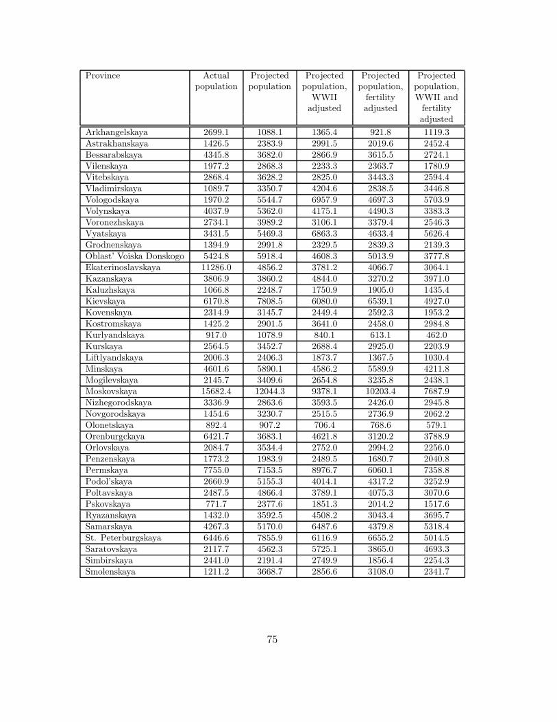
Province Actual Projected Projected Projected Projectedpopulation population population, population, population,

WWII fertility WWII andadjusted adjusted fertility

adjustedArkhangelskaya 2699.1 1088.1 1365.4 921.8 1119.3Astrakhanskaya 1426.5 2383.9 2991.5 2019.6 2452.4Bessarabskaya 4345.8 3682.0 2866.9 3615.5 2724.1Vilenskaya 1977.2 2868.3 2233.3 2363.7 1780.9Vitebskaya 2868.4 3628.2 2825.0 3443.3 2594.4Vladimirskaya 1089.7 3350.7 4204.6 2838.5 3446.8Vologodskaya 1970.2 5544.7 6957.9 4697.3 5703.9Volynskaya 4037.9 5362.0 4175.1 4490.3 3383.3Voronezhskaya 2734.1 3989.2 3106.1 3379.4 2546.3Vyatskaya 3431.5 5469.3 6863.3 4633.4 5626.4Grodnenskaya 1394.9 2991.8 2329.5 2839.3 2139.3Oblast’ Voiska Donskogo 5424.8 5918.4 4608.3 5013.9 3777.8Ekaterinoslavskaya 11286.0 4856.2 3781.2 4066.7 3064.1Kazanskaya 3806.9 3860.2 4844.0 3270.2 3971.0Kaluzhskaya 1066.8 2248.7 1750.9 1905.0 1435.4Kievskaya 6170.8 7808.5 6080.0 6539.1 4927.0Kovenskaya 2314.9 3145.7 2449.4 2592.3 1953.2Kostromskaya 1425.2 2901.5 3641.0 2458.0 2984.8Kurlyandskaya 917.0 1078.9 840.1 613.1 462.0Kurskaya 2564.5 3452.7 2688.4 2925.0 2203.9Liftlyandskaya 2006.3 2406.3 1873.7 1367.5 1030.4Minskaya 4601.6 5890.1 4586.2 5589.9 4211.8Mogilevskaya 2145.7 3409.6 2654.8 3235.8 2438.1Moskovskaya 15682.4 12044.3 9378.1 10203.4 7687.9Nizhegorodskaya 3336.9 2863.6 3593.5 2426.0 2945.8Novgorodskaya 1454.6 3230.7 2515.5 2736.9 2062.2Olonetskaya 892.4 907.2 706.4 768.6 579.1Orenburgckaya 6421.7 3683.1 4621.8 3120.2 3788.9Orlovskaya 2084.7 3534.4 2752.0 2994.2 2256.0Penzenskaya 1773.2 1983.9 2489.5 1680.7 2040.8Permskaya 7755.0 7153.5 8976.7 6060.1 7358.8Podol’skaya 2660.9 5155.3 4014.1 4317.2 3252.9Poltavskaya 2487.5 4866.4 3789.1 4075.3 3070.6Pskovskaya 771.7 2377.6 1851.3 2014.2 1517.6Ryazanskaya 1432.0 3592.5 4508.2 3043.4 3695.7Samarskaya 4267.3 5170.0 6487.6 4379.8 5318.4St. Peterburgskaya 6446.6 7855.9 6116.9 6655.2 5014.5Saratovskaya 2117.7 4562.3 5725.1 3865.0 4693.3Simbirskaya 2441.0 2191.4 2749.9 1856.4 2254.3Smolenskaya 1211.2 3668.7 2856.6 3108.0 2341.7

75

Province Actual Projected Projected Projected Projectedpopulation population population, population, population,

WWII fertility WWII andadjusted adjusted fertility

adjustedTavricheskaya 4916.7 3263.3 2540.9 2732.8 2059.1Tambovskaya 2502.7 4294.4 5389.0 3638.1 4417.7Tverskaya 1581.4 4129.1 3215.1 3498.0 2635.6Tul’skaya 1891.4 2825.5 2200.0 2393.6 1803.5Ufimskaya 4533.7 3990.1 5007.1 3380.3 4104.7Khar’kovskaya 4830.8 5352.8 4167.8 4482.6 3377.4Khersonskaya 4524.1 4397.6 3424.1 3682.7 2774.8Chernigovskaya 2317.2 4715.1 3671.3 3948.6 2975.1Estlyandskaya 1037.9 487.7 379.7 264.2 199.1Yaroslavskaya 1384.1 2207.7 2770.4 1870.3 2271.1Bakinskaya 4158.6 1674.7 2101.5 2761.1 3352.8Batumskaya 392.7 133.3 167.2 156.6 190.2Dagestanskaya 1514.1 864.3 1084.5 1424.9 1730.3Elisavetpol’skaya 2536.2 2301.0 2887.4 3793.7 4606.7Kubanskaya 4929.3 6013.9 4682.7 5094.8 3838.7Kutaisskaya 1441.9 1536.8 1928.5 1806.1 2193.1Stavropol’skaya 1685.1 1986.0 1546.3 1682.4 1267.6Terskaya 4209.6 3367.4 2622.0 5551.9 4183.2Tiflisskaya 2898.9 3456.8 4337.8 4062.4 4933.0Chernomorskaya 585.7 157.3 197.4 133.3 161.9Erivanskaya 3582.8 1715.6 2152.9 3498.5 4248.3Amurskaya 1333.4 498.0 625.0 421.9 512.3Eniseiskaya 4244.4 3234.7 4059.2 2740.3 3327.6Zabaikal’skaya 2496.1 1180.7 1481.7 1000.3 1214.6Irkutskaya 2966.9 1675.9 2103.0 1419.7 1724.0Primorskaya 5009.5 731.9 918.4 620.0 752.9Sakhalinskaya 709.6 22.5 28.2 19.0 23.1Tobol’skaya 6245.8 5688.5 7138.4 4819.1 5851.8Tomskaya 10160.8 6112.0 7669.8 5177.8 6287.5Yakutskaya 1081.4 527.3 661.6 446.7 542.4Akmolinskaya 5449.1 2272.0 2851.0 3611.3 4385.3Zakaspiiskaya 2424.1 1765.1 2214.9 3810.5 4627.0Samarkandskaya 2290.9 2181.8 2737.9 5060.4 6144.8Semipalatinskaya 2576.7 1866.8 2342.6 2967.4 3603.3Semirechenskaya 6489.2 2211.0 2774.5 3920.6 4760.8Syr-Dar’inskaya 7971.0 6433.8 8073.5 14922.1 18120.0Turgaiskaya 1629.8 1522.6 1910.7 2420.2 2938.9Ural’skaya 1102.0 2125.1 2666.7 3377.8 4101.7Ferganskaya 10466.4 5948.8 7465.0 12310.0 14948.0

Table C.4: Projected vs actual population. Russia.

76

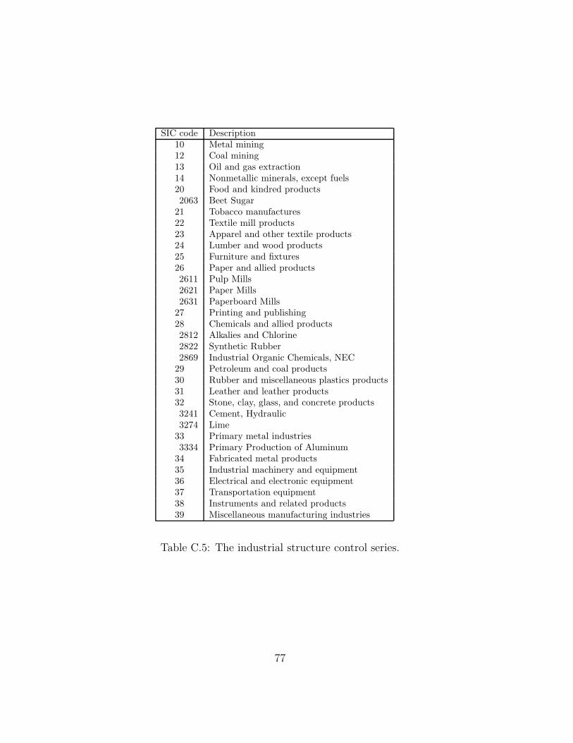
SIC code Description10 Metal mining12 Coal mining13 Oil and gas extraction14 Nonmetallic minerals, except fuels20 Food and kindred products2063 Beet Sugar

21 Tobacco manufactures22 Textile mill products23 Apparel and other textile products24 Lumber and wood products25 Furniture and fixtures26 Paper and allied products2611 Pulp Mills2621 Paper Mills2631 Paperboard Mills

27 Printing and publishing28 Chemicals and allied products2812 Alkalies and Chlorine2822 Synthetic Rubber2869 Industrial Organic Chemicals, NEC

29 Petroleum and coal products30 Rubber and miscellaneous plastics products31 Leather and leather products32 Stone, clay, glass, and concrete products3241 Cement, Hydraulic3274 Lime

33 Primary metal industries3334 Primary Production of Aluminum

34 Fabricated metal products35 Industrial machinery and equipment36 Electrical and electronic equipment37 Transportation equipment38 Instruments and related products39 Miscellaneous manufacturing industries

Table C.5: The industrial structure control series.

77

Dependent variable is Log of industrial electicityIndependent consumption per unit of labor in 1991Variables VPK no VPK VPK no VPK VPK no VPKTemperature -0.039* -0.041* -0.037* -0.40* -0.037* -0.040*

(0.006) (0.006) (0.007) (0.006) (0.006) (0.006)SIC10 -0.27 -2.59

(2.07) (2.05)SIC12,14 -2.39* -5.20* -2.28* -1.72

(1.01) (1.93) (0.82) (1.08)SIC13 5.30* 2.08 5.41* 4.71*

(1.23) (1.84) (0.67) (0.65)SIC20 -0.69 -4.06*

(1.04) (2.03)SIC2063 -1.04 -3.26 -1.84 -1.25

(4.39) (3.17) (3.84) (3.12)SIC22-25 -2.76* -4.63* -2.49* -1.69*

(1.23) (1.79) (0.72) (0.84)SIC26,2631 -10.28* -10.28* -12.28* -10.56*

(5.02) (4.36) (4.37) (4.42)SIC2611 9.59 2.34 9.21 6.91

(6.00) (5.69) (4.83) (4.11)SIC2621 -0.91 -5.77

(1.59) (3.12)SIC27 1.97 1.39

(8.62) (7.15)SIC28 2.26 -0.84 3.09* 2.11

(1.67) (1.92) (1.42) (1.19)SIC2822 20.35* 12.11* 18.48* 12.10*

(5.45) (3.10) (4.85) (2.34)SIC2869 2.60 -1.27

(3.63) (3.08)SIC29,30 -3.96* -6.36* -2.85* -2.49*

(1.30) (2.11) (0.97) (1.09)SIC31 0.52 -2.53

(5.23) (4.38)SIC33 0.09 -2.65

(1.23) (1.86)SIC3334 16.65* 10.25* 16.04* 13.55*

(4.91) (4.02) (4.08) (3.71)SIC3241 14.23 9.48 11.90 8.42

(9.36) (8.17) (8.54) (7.37)SIC32,34-38 - -4.42* -1.24

(1.83) (0.75)SIC32,34-38, -2.60* -2.41*VPK (1.16) (0.61)SIC39 3.63 1.11

(4.06) (3.45)R2 0.22 0.26 0.79 0.74 0.77 0.66No. of obs 75 75 75 75 75 75

Heteroskedasticity-consistent standard errors are in parentheses,* denotes significance on the 95% level.

Table C.6: Electricity in 1991.

78

Dependent variable is Log of industrial electicityIndependent consumption per unit of labor in 1992Variables VPK no VPK VPK no VPK VPK no VPKTemperature -0.039* -0.040* -0.038* -0.040* -0.038* -0.041*

(0.007) (0.007) (0.007) (0.006) (0.007) (0.006)SIC10 0.17 -2.30

(1.51) (1.71)SIC12,14 -0.93 -4.11* -1.28 -1.23

(1.04) (1.81) (0.86) (1.04)SIC13 6.65* 2.91 6.04* 4.95*

(1.48) (1.84) (0.72) (0.69)SIC20 -0.34 -3.75

(1.24) (2.16)SIC2063 8.87* 3.61 6.45 4.01

(4.26) (3.55) (4.06) (3.70)SIC22-25 -1.63 -3.98* -1.96* -1.58*

(1.32) (1.79) (0.55) (0.72)SIC26,2631 -7.07 -8.86* -8.66 -8.54*

(6.14) (4.16) (5.09) (3.46)SIC2611 6.10 -0.49 6.10 3.78

(6.40) (5.37) (5.41) (4.19)SIC2621 0.25 -4.83

(2.05) (2.66)SIC27 7.79 5.46

(9.94) (7.37)SIC28 2.61 -0.64 3.09* 2.10

(1.96) (1.95) (1.50) (1.09)SIC2822 16.40* 9.54* 13.19* 8.53*

(6.28) (3.60) (5.59) (2.73)SIC2869 1.05 -2.41

(4.72) (3.10)SIC29,30 -1.21 -4.19* -1.05 -1.06

(1.74) (2.06) (1.23) (1.10)SIC31 -3.57 -6.05

(4.24) (4.07)SIC33 1.39 -1.77

(1.43) (1.86)SIC3334 20.00* 12.04* 18.05* 14.59*

(4.88) (3.70) (4.60) (3.84)SIC3241 0.089 -4.61 -4.87 -6.12

(6.17) (6.24) (5.29) (6.32)SIC32,34-38 -3.80* -1.17

(1.80) (0.68)SIC32,34-38, -1.51 -1.87VPK (1.26) (0.48)SIC39 4.96 1.76

(4.62) (3.68)R2 0.21 0.24 0.74 0.72 0.71 0.64No. of obs 79 79 79 79 79 79

Heteroskedasticity-consistent standard errors are in parentheses,* denotes significance on the 95% level.

Table C.7: Electricity in 1992.

79

Dependent variable is Log of industrial thermal energyIndependent consumption per unit of labor in 1991Variables VPK no VPK VPK no VPK VPK no VPKTemperature -0.025* -0.027* -0.019* -0.23* -0.026* -0.024*

(0.007) (0.007) (0.009) (0.008) (0.007) (0.007)SIC10 2.13 -0.16

(2.24) (2.71)SIC12,14 1.04 -0.69

(1.48) (2.46)SIC13 3.73* 2.10 3.72* 2.44*

(1.85) (2.58) (0.82) (0.63)SIC20 -1.07 -2.23* -1.13* -1.49

(0.93) (2.57) (0.40) (0.55)SIC21 45.36* 16.79

(22.78) (19.74)SIC22-24 0.15 -0.96

(1.53) (2.55)SIC25,2063 1.51 0.42 2.81 1.99

(2.61) (3.06) (1.79) (0.84)SIC26 -45.65* -41.48* -41.44* -39.08*

(17.39) (18.24) (13.53) (15.99)SIC2611 12.22 5.92 8.32 7.20

(6.36) (7.18) (5.03) (3.97)SIC2621 3.33 1.70 3.55 2.02

(3.41) (4.00) (2.43) (2.02)SIC2631 1.09 -0.94

(8.63) 6.42SIC27 1.62 3.78 6.00 8.30

(7.07) (5.95) (5.04) (4.79)SIC28,29 5.09* 2.85 5.33* 3.55*

(2.23) (2.59) (1.45) (1.19)SIC2822,2869 17.68* 12.00* 15.36* 13.66*

(3.60) (2.92) (3.21) (2.59)SIC30-32 0.10 1.10

(2.27) (3.07)SIC33 1.25 0.19 1.63 0.90

(1.65) (2.58) (0.59) (0.53)SIC3334 4.89 2.55 7.69 3.53

(4.17) (4.30) (4.41) (3.61)SIC3241 -0.01 3.30

(11.34) (9.56)SIC34-35,37-38 - -0.95* -

(2.46)SIC34-35,37-38, 0.08 - -VPK (1.51)

SIC36 1.09 -1.87 -1.35 -1.02(1.62) (2.44) (0.66) (0.64)

SIC39 3.11 1.32(3.86) (3.54)

R2 0.11 0.11 0.69 0.64 0.65 0.61No. of obs 75 75 75 75 75 75

Heteroskedasticity-consistent standard errors are in parentheses,* denotes significance on the 95% level.

Table C.8: Thermal energy in 1991.

80

Dependent variable is Log of industrial thermal energyIndependent consumption per unit of labor in 1992Variables VPK no VPK VPK no VPK VPK no VPKTemperature -0.035* -0.036* -0.039* -0.041* -0.044* -0.042*

(0.007) (0.007) (0.007) (0.007) (0.006) (0.006)SIC10 0.59 -1.29

(1.20) (1.74)SIC12,14 -1.05 -2.94

(0.87) (1.84)SIC13 2.43 0.60 3.26* 2.26*

(1.35) (1.89) (0.67) (0.58)SIC20 -0.32 -2.37 0.55 0.10

(0.66) (1.74) (0.37) (0.44)SIC21 5.44 -3.17

(24.96) (18.42)SIC22-24 -1.15 -2.64

(1.05) (1.78)SIC25,2063 -1.73 -3.98* -3.44* -2.42

(2.17) (1.79) (1.55) (1.71)SIC26 9.72 -1.87 -1.39 -1.28

(11.99) (11.89) (8.05) (9.67)SIC2611 7.59 -1.73 7.02 6.14

(4.60) (5.18) (4.62) (3.87)SIC2621 3.49 0.72 4.51* 3.00

(2.08) (2.65) (1.18) (1.12)SIC2631 -2.48 -1.93

(7.38) (4.65)SIC27 -13.45* -6.84 -7.34 -2.59

(5.90) (4.81) (5.60) (4.32)SIC28,29 2.86 0.96 4.12* 2.86*

(1.78) (1.84) (1.42) (1.11)SIC2822,2869 12.39* 7.31* 12.95* 11.18*

(3.58) (2.80) (3.13) (2.39)SIC30-32 -0.19 -0.17

(2.02) (1.98)SIC33 0.26 -1.13 1.34* 0.83

(1.22) (1.77) (0.54) (0.49)SIC3334 2.26 -0.86 5.22 2.07

(3.54) (3.28) (4.11) (3.55)SIC3241 6.13 1.18

(5.80) (4.67)SIC34-35,37-38 - -2.61 -

(1.74)SIC34-35,37-38, -1.13 - -VPK (1.00)

SIC36 -2.35 -3.47* -1.04 -0.90(1.13) (1.74) (0.72) (0.58)

SIC39 0.05 -1.42(3.59) (3.23)

R2 0.27 0.26 0.73 0.66 0.71 0.58No. of obs 79 79 79 79 79 79

Heteroskedasticity-consistent standard errors are in parentheses,* denotes significance on the 95% level.

Table C.9: Thermal energy in 1992.

81

Dependent variable is Log of industrial consumptionIndependent of fuel per unit of labor in 1991Variables VPK no VPK VPK no VPK VPK no VPKTemperature -0.042* -0.044* -0.025* -0.026* -0.029* -0.026*

(0.008) (0.008) (0.008) (0.008) (0.007) (0.007)SIC10 0.23 -1.00

(1.86) (1.92)SIC12,14 -0.50 -1.83

(0.73) (1.23)SIC13 7.07* 4.74* 7.17* 5.94*

(1.10) (1.17) (0.63) (0.49)SIC20,21,24 0.51 -0.96 0.67 0.32

(0.62) (1.19) (0.52) (0.49)SIC2063 -12.66* -11.44* -9.55* -8.51*

(5.26) (3.58) (2.77) (1.84)SIC22-23 -1.35* -2.40 -0.99* -1.12*

(0.69) (1.14) (0.46) (0.47)SIC25 -7.00* -6.43* -5.30* -4.95*

(2.58) (2.69) (1.69) (2.09)SIC26,2631 5.41 0.68

(4.61) (3.47)SIC2611,2621 -1.55 -2.49

(1.94) (2.20)SIC27 10.62 7.30 9.65 8.55

(8.19) (5.98) (5.54) (4.75)SIC28-29 6.47* 3.61* 6.52* 4.58*

(2.09) (1.63) (1.88) (1.23)SIC2822 17.62* 10.18* 19.68* 13.11*

(7.06) (4.74) (7.39) (4.42)SIC2869 -4.48 -2.91

(9.16) (5.24)SIC30-31 1.11 0.05

(2.53) (1.80)SIC32 1.37 1.28 1.34 2.39

(2.32) (1.46) (1.97) (1.48)SIC3241 21.61* 13.89 22.93* 15.74*

(10.64) (8.38) (10.20) (7.61)SIC3274 -72.61 -39.68

(61.83) (48.43)SIC33 2.79* 0.99 2.91* 2.06*

(0.84) (1.08) (0.63) (0.49)SIC3334 -6.82* -7.88* -5.90* -5.79*

(3.45) (3.02) (2.89) (2.71)SIC34,36,38 -3.25* -3.62* -2.69* -2.14*

(0.95) (1.20) (0.69) (0.53)SIC35,37,VPK -1.04 - -0.69* -

(0.68) (0.35)SIC35,37 - -1.95 - -0.35

(1.16) (0.39)SIC39 -4.46 -3.57

(6.09) (3.84)R2 0.20 0.23 0.77 0.76 0.76 0.74No. of obs 75 75 75 75 75 75

Heteroskedasticity-consistent standard errors are in parentheses,* denotes significance on the 95% level.

Table C.10: Fuels in 1991.

82

Dependent variable is Log of industrial consumptionIndependent of fuel per unit of labor in 1992Variables VPK no VPK VPK no VPK VPK no VPKTemperature -0.049* -0.049* -0.034* -0.034* -0.037* -0.036*

(0.009) (0.008) (0.006) (0.008) (0.006) (0.006)SIC10 0.75 -0.10

(0.64) (0.78)SIC12,14 -0.67 -0.61

(0.62) (0.78)SIC13 6.95* 4.99* 6.67* 5.63*

(0.97) (0.78) (0.57) (0.41)SIC20,21,24 0.58 -0.68 0.07 -0.39

(0.36) (0.82) (0.45) (0.39)SIC2063 -9.56* -8.57* -8.83* -6.56*

(4.11) (3.50) (3.21) (2.89)SIC22-23 -1.11* -1.94* -1.47* -1.39*

(0.43) (0.77) (0.34) (0.36)SIC25 -3.83 -3.98* -4.34* -3.42*

(2.10) (1.79) (1.73) (1.71)SIC26,2631 -0.83 -3.48

(3.69) (2.80)SIC2611,2621 -0.82 -1.88

(1.17) (1.73)SIC27 9.96 6.97 10.65 7.74

(7.61) (5.50) (5.50) (4.14)SIC28-29 6.94* 4.26* 6.66* 4.61*

(1.89) (1.41) (1.54) (1.13)SIC2822 20.53* 10.56 21.26* 11.41*

(6.80) (4.38) (6.50) (3.66)SIC2869 1.08 1.04

(8.06) (4.18)SIC30-31 0.90* -0.05

(1.94) (1.49)SIC32 2.38 1.37 2.26 1.91

(1.79) (1.24) (1.61) (1.01)SIC3241 3.95 0.71 3.94 1.52

(5.21) (4.88) (4.44) (4.31)SIC3274 -39.71 -14.71

(58.64) (45.26)SIC33 3.46* 1.67* 3.03* 2.07

(0.66) (0.80) (0.55) (0.44)SIC3334 -8.54* -8.94* -9.49* -8.31*

(3.07) (2.53) (2.53) (2.28)SIC34,36,38 -2.80* -3.13* -3.23* -2.70*

(0.72) (0.77) (0.58) (0.40)SIC35,37,VPK -1.00* - -1.44* -

(0.48) (0.27)SIC35,37 - -1.74* - -1.20*

(0.83) (0.37)SIC39 -0.40 -1.27

(5.59) (3.56)R2 0.26 0.28 0.81 0.79 0.81 0.78No. of obs 79 79 79 79 79 79

Heteroskedasticity-consistent standard errors are in parentheses,* denotes significance on the 95% level.

Table C.11: Fuels in 1992.

83

Bibliography

Abele, G. (1986), Effect of Cold Weather on Productivity, in ‘Technology Trans-fer Opportunities for the Construction Engineering Community. Proceedings ofConstruction Seminar.’, US Army Cold Regions Research and Engeneering Lab-oratory.

Acemoglu, D., Johnson, S. & Robinson, J. (2002), ‘Reversal of Fortune: Geogra-phy and Institutions in the making of the Modern World’, Quarterly Journal ofEconomics 117.

Barro, R. J. & Sala-i-Martin, X. (1995), Economic Growth, McGraw-Hill, New York,NY.

Bloom, D. & Sachs, J. D. (1998), ‘Geography, Demography and Growth in Africa’,Brookings Papers on Economic Activity 2.

Carlton, D. W. (1983), ‘The Location and Employment Choices of New Firms: AnEconometric Model with Discrete and Continuous Endogenous Variables’, TheReview of Economics and Statistics 65, 440–449.

Davis, D. R. & Weinstein, D. E. (2001), ‘Bones, Bombs, and Break Points: TheGeography of Economic Activity’, NBER working paper 8517.

Fogel, R. W. (1964), Railroads and American Economic Growth: Essays in Econo-metric History, Johns Hopkins University Press, Baltimore, Maryland.

Fujita, M., Krugman, P. & Venables, A. J. (2000), The Spatial Economy: Cities,Regions, and International Trade, The MIT Press, Cambridge, Massachusetts.

Gaddy, C. G. (1996), The Price of the Past: Russia’s Struggle with the Legacy of aMilitarized Economy, Brookings Institution Press, Washington, D.C.

Gaddy, C. G. & Ickes, B. W. (2001), ‘The Cost of the Cold’, The Pennsylvania StateUniversity working paper, unpublished.

Gallup, J. L., Sachs, J. D. & Mellinger, A. (1999), ‘Geography and Economic Devel-opment’, International Regional Science Review 22(2), 179–232.

84

Gluschenko, K. (2002), ‘Common Russian Market: Myth rather than Reality’, Eco-nomic Education and Research Consortium Working Paper Series .

Heleniak, T. (1999), ‘Out-Migration and Depopulation of the Russian North duringthe 1990s’, Eurasian Geography and Economics 40, 155–205.

Herbert, D. & Burton, I. (1994), Estimated Costs of Adaptation to Canada’s CurrentClimate and Trends Under Climate Change. Atmospheric Environment Service,unpublished.

Hill, F. & Gaddy, C. (2003), The Siberian Curse. How Communist Planners LeftRussia Out in the Cold., Brookings Institution Press, Washington, DC. forth-coming.

Horrigan, B. (1992), ‘How Many People Worked in Soviet Defense Industry?’,RFE/RL Report 1(33).

Islam, N. (1995), ‘Growth Empirics: A Panel Data Approach’, Quarterly Journal ofEconomics 110.

Lynch, A. C. (2002), ‘Roots of Russia’s Economic Dilemmas: Liberal Economics andIlliberal Geography’, Europe-Asia Studies 154, 31–49.

Masters, W. & McMillan, M. (2000), ‘Climate and Scale in Economic Growth’, CIDworking paper No. 48.

Mikhailova, T. (2003), Where Russians Should Live: a Counterfactual Alternative toSoviet Location Policy. The Pennsylvania State University, unpublished.

North, D. C. (1990), Institutions, Institutional Change, and Economic Performance,Cambridge University Press, New York, NY.

Olkhovsky, G. (2001), ‘Combined Electricity and Heat Generation in Russia: EfficientWay of Greening Fossil Fuels’, Towards Local Energy Systems: Revitalizing Dis-trict Heating and Co-Generation in Central and Eastern Europe. World EnergyCouncil conference report. .

Parshev, A. P. (1999), Why Russia is not America, Forum, Moscow.

Rappaport, J. & Sachs, J. D. (2001), ‘US as a Coastal Nation’, Research Division,Federal Researve Bank of Kansas City.

Rosen, K. T. (1979), Seasonal Cycles in the Housing Market, The MIT Press, Cam-bridge, MA.

Rosenthal, D. H., Gruenspecht, H. & Moran, E. A. (1995), ‘Effect of Global Warmingon Energy Use for Space Heating and Cooling in the United States’, The EnergyJournal 16(2).

85

Vassin, S. A. & Costello, C. A. (1997), Spatial, Age, and Cause-of-Death Patterns ofMortality in Russia, 1988-1989, in ‘Premature Death in the New IndependentStates’, The National Academy of Science.

86

Vita

Date & Place of Birth: 22 Nov 1973; Moscow, Russia

Citizenship: Russian Federation

Education: 2004, Ph.D. in Economics, Pennsylvania State University

1997, M.A. in Economics (cum laude), New Economic School, Moscow, Russia

1996, Diplom in Electronic Engineering, Moscow State Institute of ElectronicEngineering, Russia

Fields: Primary: Economics of Transition

Secondary: Industrial Organization, International Trade

Presentations: “Regional Migration in Russia,” presented at GET Conference, NewEconomic School, Moscow, Russia, 1997

“Where Russians Should Live: A Counterfactual Alternative to Soviet LocationPolicy,” presented at Cornell-PSU Macro Workshop, 2001; the VIIth SMYEConference, 2002; Midwest International Economics Meeting, 2002; Compara-tive Economics Seminar at the Davis Center for Russian and Eastern EuropeanStudies, Harvard University, 2003; CEFIR open seminar, Moscow, 2003

Experience: Instructor (visiting), Intermediate Macroeconomics, Fall(I) 2003, NewEconomic School, Moscow

Instructor, Intermediate Microeconomics, Summer 2000

Research Assistant for Professor Kala Krishna, Summer 1998

Teaching Assistant for Microeconomic Theory (graduate), Mathematics for Economists(graduate), International Finance, Labor Economics, Monetary Theory andPolicy, Intermediate Microeconomics, Introductory Microeconomics, Fall 1997–Spring 2001

Member of the research group, Government and Economy in Transition (GET)project, New Economic School, Moscow, Russia, 1996-1997