essays on service strategies: evidence from banking and
TRANSCRIPT

Clemson UniversityTigerPrints
All Dissertations Dissertations
8-2013
Essays on Service Strategies: Evidence fromBanking and Healthcare IndustriesSriram VenkataramanClemson University, [email protected]
Follow this and additional works at: https://tigerprints.clemson.edu/all_dissertations
Part of the Management Sciences and Quantitative Methods Commons
This Dissertation is brought to you for free and open access by the Dissertations at TigerPrints. It has been accepted for inclusion in All Dissertations byan authorized administrator of TigerPrints. For more information, please contact [email protected].
Recommended CitationVenkataraman, Sriram, "Essays on Service Strategies: Evidence from Banking and Healthcare Industries" (2013). All Dissertations.1188.https://tigerprints.clemson.edu/all_dissertations/1188

Essays on Service Strategies:Evidence from Banking and Healthcare
Industries
A Dissertation
Presented to
the Graduate School of
Clemson University
In Partial Fulfillment
of the Requirements for the Degree
Doctor of Philosophy
Management
by
Sriram Venkataraman
August 2013
Accepted by:
Dr. Aleda V. Roth, Committee Co-Chair
Dr. Lawrence D. Fredendall, Committee Co-Chair
Dr. Shouqiang Wang
Dr. Paul W. Wilson
Dr. Daniel P. Miller
Abstract
The primary objective of this dissertation is to provide insights for service
providers in general, and retail bankers and hospital administrators in particular,
that will help them improve their operational efficiency and effectiveness. In doing
so, this dissertation consists of three essays that develop multiple service operations
strategies, that identifies key elements affecting efficiency and effectiveness in two
key critical industries: banking and healthcare. We contribute to service operations
strategy research and practice by incorporating multi-disciplinary theories and ap-
proaches from marketing, economics, and quality management. Although operations
researchers and practitioners alike realize the importance of productivity and effec-
tiveness, they are largely unaware of more advanced techniques to achieve this goal.
This dissertation fills, in part, this gap and leads one to understand research agendas
in service strategy. In particular, this dissertation applies new theories and methods
illustrating how bankers can improve efficiency. Moreover, it describes how hospital
administrators can better understand the ‘hidden’ costs of quality failures that asso-
ciated with hospital readmission as well as the impact of the recent Medicare penalty
plan on hospitals and patient welfare. We employ different methods (frontier effi-
ciency estimation, econometrics, structural estimation, and principal-agent models)
to critically analyze banking and healthcare industries.
The first essay deals with banking industry; the second and third essays are
ii

inter-related topics dealing with healthcare services. The first essay integrates diffu-
sion theory from marketing literature and path dependency theory from economics
into service operations management to estimate and compare efficiency of banks op-
erating in the U.S. and in India. We develop and empirically test two hypotheses
based on diffusion theory and path dependency theory. The hypotheses are tested
using data from banks operating in the U.S. and India and estimate efficiency us-
ing free disposal hull (FDH) estimator instead of the widely used data envelopment
analysis (DEA) estimator. We note that the DEA estimator imposes convexity of
production frontier whereas FDH estimator does not. Our empirical analysis, reject-
ed the assumption of convexity of production frontier; and we are the first in the
operations management literature to employ these empirics to test assumptions that
are typically held to be true, but not validated, when employing DEA analyses.
The second essay develops a theory-based econometric model to investigate
the effect of readmission rate on marginal cost incurred by a hospital. We use sec-
ondary data derived from multiple sources, including Center for Medicare and Med-
icaid Services. We apply an inversion method and structural estimation procedure
developed in the empirical Industrial Organization and econometrics literature to
estimate marginal cost of a hospital associated with readmissions using data on all
Arizona hospitals. This essay also demonstrates the effect of the recent Medicare
penalty on average readmission rate of all hospitals in the state of Arizona by using
counterfactual analysis with and without stochastic shocks in hospitals’ investment
to reduce readmission rates. The revised price charged by acute care hospitals after
the elimination of critical access hospitals is also estimated as another counterfactual
analysis. These analyses are very timely since patient protection and affordable care
act (PPACA) was enacted recently, which penalizes hospitals with readmission rates
higher than threshold readmission rates set by the government. Thus, in addition to
iii

research and practice, this essay offers strong policy insights.
The third essay formulates an analytical model to evaluate the potential impact
of PPACA on hospitals (providers), the government, and patients. We build a model
of “readmission” with uncertainty for hospitals and use the principal-agent frame work
to study the interaction between the government (principal) and the hospital (agent).
The hospital can make effort to reduce the readmission rate (hidden action). The
hospital side is modeled using queueing with feedback results. Finally, we evaluate
the impact of hospital’s efforts on the government’s expense and patient welfare.
iv

Dedication
This dissertation is dedicated to my parents.
v

Acknowledgments
I would not have completed my pursuit of Doctor of Philosophy degree with-
out the help of many people. I would like to take this opportunity to thank all of
them. I express deep gratitude to my dissertation co-chair, Dr. Aleda Roth for her
constant support, guidance and encouragement which helped me strive high levels of
excellence. Her enthusiasm for research is very infectious. I also would like to thank
my dissertation co-chair, Dr. Larry Fredendall for his immense help and support over
the past four years and for providing me an opportunity to be part of the healthcare
research project. I am extremely grateful to Dr. Paul Wilson for his patience in an-
swering all my questions, his help on the first essay of this dissertation and in teaching
the econometrics courses. I would like to thank Dr. Shouqiang Wang for his constant
support and help during my research especially for the third essay of this dissertation.
I would also like to thank Dr. Daniel Miller for all his help on the second essay of
this dissertation and for teaching the Advanced Industrial Organization class.
I would like to thank the other faculty members of Supply Chain and Opera-
tions group: Dr. V. Sridharan, Dr. Janis Miller, Dr. Yann Ferrand and Dr. Gulru
Ozkan for their support throughout my Ph.D. program. I express my gratitude to my
colleagues Jason Riley, Kevin Craig, Enrico Secchi, David Hall, Tracy Johnson-Hall,
Jill Davis and Qiong Chen for their inspiration. Thanks also go to my friends Jud-
hajit Roy, Shyam Panyam, Durlove Mohanty, Mandar Hazare and Rajat Aggarwal
vi

for their help during my stay in Clemson. Finally, I would like thank my parents and
my brother. This dissertation would not have been possible without their constant
support and inspiration.
vii

Table of Contents
Title Page . . . . . . . . . . . . . . . . . . . . . . . . . . . . . . . . . . . i
Abstract . . . . . . . . . . . . . . . . . . . . . . . . . . . . . . . . . . . . ii
Dedication . . . . . . . . . . . . . . . . . . . . . . . . . . . . . . . . . . . v
Acknowledgments . . . . . . . . . . . . . . . . . . . . . . . . . . . . . . . vi
List of Tables . . . . . . . . . . . . . . . . . . . . . . . . . . . . . . . . . x
List of Figures . . . . . . . . . . . . . . . . . . . . . . . . . . . . . . . . . xi
Introduction . . . . . . . . . . . . . . . . . . . . . . . . . . . . . . . . . . 1
Essay 1: Efficiency Analysis of U.S. and Indian Banks: Theory andEvidence . . . . . . . . . . . . . . . . . . . . . . . . . . . . . . . . . . 61.1 Introduction . . . . . . . . . . . . . . . . . . . . . . . . . . . . . . . . 71.2 Literature Review . . . . . . . . . . . . . . . . . . . . . . . . . . . . . 91.3 Hypotheses . . . . . . . . . . . . . . . . . . . . . . . . . . . . . . . . 121.4 Research Approach . . . . . . . . . . . . . . . . . . . . . . . . . . . . 151.5 Results . . . . . . . . . . . . . . . . . . . . . . . . . . . . . . . . . . . 231.6 Conclusions and Limitations . . . . . . . . . . . . . . . . . . . . . . . 29
Essay 2. Effect of Readmission Rates on Marginal Cost in HospitalServices: An Econometric Analysis . . . . . . . . . . . . . . . . . . 322.1 Introduction . . . . . . . . . . . . . . . . . . . . . . . . . . . . . . . . 332.2 Literature and Hypothesis Development . . . . . . . . . . . . . . . . 392.3 Data . . . . . . . . . . . . . . . . . . . . . . . . . . . . . . . . . . . . 442.4 Econometric Model and Estimation Procedure . . . . . . . . . . . . . 462.5 Results and Discussion . . . . . . . . . . . . . . . . . . . . . . . . . . 522.6 Conclusions . . . . . . . . . . . . . . . . . . . . . . . . . . . . . . . . 69
Essay 3. Hospital and Patient Incentives to Reduce ReadmissionRates: A Quality Management Framework . . . . . . . . . . . . . . 73
viii

3.1 Introduction . . . . . . . . . . . . . . . . . . . . . . . . . . . . . . . . 743.2 Literature Review . . . . . . . . . . . . . . . . . . . . . . . . . . . . . 783.3 Model . . . . . . . . . . . . . . . . . . . . . . . . . . . . . . . . . . . 813.4 Results . . . . . . . . . . . . . . . . . . . . . . . . . . . . . . . . . . . 853.5 Conclusions . . . . . . . . . . . . . . . . . . . . . . . . . . . . . . . . 88
Conclusions . . . . . . . . . . . . . . . . . . . . . . . . . . . . . . . . . . 91
Appendices . . . . . . . . . . . . . . . . . . . . . . . . . . . . . . . . . . . 95A Proofs of Theorems in Essay 3 . . . . . . . . . . . . . . . . . . . . . . 96B Codes of Computer Programs . . . . . . . . . . . . . . . . . . . . . . 102
Bibliography . . . . . . . . . . . . . . . . . . . . . . . . . . . . . . . . . . 130
ix

List of Tables
1.1 Descriptive Statistics of Variables (N = 6535) . . . . . . . . . . . . . 161.2 Descriptive Statistics of FDH Estimates . . . . . . . . . . . . . . . . 241.3 Descriptive Statistics of FDH Estimates of Indian Banks . . . . . . . 252.1 Descriptive Statistics . . . . . . . . . . . . . . . . . . . . . . . . . . . 452.2 Non-Nested Model: OLS Estimates [DV: log(sj)− log(s0)] . . . . . . 522.3 Non-Nested Model: IV Estimates [DV: log(sj)− log(s0)] . . . . . . . 532.4 Summary Statistics of Non-Nested Model . . . . . . . . . . . . . . . 542.5 Nested Model: OLS Estimates [DV: log(sj)− log(s0)] . . . . . . . . . 542.6 Nested Model: IV Estimates [DV: log(sj)− log(s0)] . . . . . . . . . . 552.7 Summary Statistics of Nested Model . . . . . . . . . . . . . . . . . . 562.8 Nested Model: Supply Side Estimates [DV: Marginal Cost] . . . . . . 562.9 Nested Model (Not for Profit): Supply Side Estimates [DV: Marginal
Cost] . . . . . . . . . . . . . . . . . . . . . . . . . . . . . . . . . . . 573.1 Notation Table . . . . . . . . . . . . . . . . . . . . . . . . . . . . . . 833.2 Numerical Values . . . . . . . . . . . . . . . . . . . . . . . . . . . . . 86
x

List of Figures
0.1 Overview of the Dissertation . . . . . . . . . . . . . . . . . . . . . . . 22.1 Illustrative Example of Payment Scheme for Penalized and Unpenal-
ized Hospitals . . . . . . . . . . . . . . . . . . . . . . . . . . . . . . . 352.2 Influence of Quadratic Cost Coefficient on Number of Hospitals Re-
ducing Readmissions . . . . . . . . . . . . . . . . . . . . . . . . . . . 622.3 Steady-State Behavior of Hospitals in Market 1 . . . . . . . . . . . . 632.4 Steady-State Behavior of Hospitals in Market 2 . . . . . . . . . . . . 642.5 Steady-State Behavior of Hospitals in Market 3 . . . . . . . . . . . . 652.6 Steady-State Behavior of Hospitals in Market 1 with Stochastic Shock 662.7 Steady-State Behavior of Hospitals in Market 2 with Stochastic Shock 672.8 Steady-State Behavior of Hospitals in Market 3 with Stochastic Shock 683.1 Profit for Two Hospitals . . . . . . . . . . . . . . . . . . . . . . . . . 763.2 Timeline . . . . . . . . . . . . . . . . . . . . . . . . . . . . . . . . . . 823.3 Queueing with Feedback . . . . . . . . . . . . . . . . . . . . . . . . . 843.4 Effect of Threshold Readmission Rate and Payment Factor on Optimal
Readmission Rate . . . . . . . . . . . . . . . . . . . . . . . . . . . . . 873.5 Effect of Threshold Readmission Rate and Payment Factor on Optimal
Patient Cost . . . . . . . . . . . . . . . . . . . . . . . . . . . . . . . . 88
xi

Introduction
This dissertation aims to find key elements that affect operational efficiency
and effectiveness in two critical service industries: banking and healthcare. In par-
ticular, this dissertation identifies key antecedents of efficiency in banking and cost
drivers which are associated with hospital readmissions that affect effectiveness in the
healthcare industry.
We draw from research in the field of Service Operations (Lewin and Minton
1986, Heskett et al. 1990, Roth and Jackson 1995, Roth and Menor 2003), Efficiency
Analysis (Farrell 1957, Charnes et al. 1978, Banker et al. 1984, Deprins et al. 1984,
Kneip et al. 2013a,b), Healthcare Operations (Roth et al. 1996, So and Tang 2000,
Fuloria and Zenios 2001, Chao et al. 2003, Green 2004, Anand et al. 2011, KC and
Terwiesch 2012, Jiang et al. 2013, Bartel et al. 2013), Quality Management (Juran
1992, Garvin 1987, Giffi et al. 1990, Chen et al. 1999, Savage and Seshadri 2003,
Alukal 2006), Structural Estimation (Berry 1994, Berry et al. 1995, Olivares et al.
2008, Allon et al. 2011, Deshpande and Arikan 2012) to comprehensively analyze
banking and healthcare industries.
This dissertation is comprised of three essays. Essay 1 deals with the banking
industry while essays 2 and 3 deal with the hospital sector. The three essays collec-
tively advance service operations strategy theory, practice, and policies, as depicted
1

in Figure 0.1.
Figure 0.1: Overview of the Dissertation
Essay 1 compares and contrasts the efficiency of banks operating in India and
in the U.S. It also compares the efficiency of banks operating within India. Diffusion
theory from marketing and path dependence theory from economics are used to de-
velop two hypotheses explaining, in part, the efficiency of banks operating in India
and in the U.S.; subsequently, comparing the efficiency of state-owned (public), do-
mestic private and foreign banks operating within India respectively. Foreign banks
have proliferated in India since the early 1990s. Arguably, foreign banks from western
countries would have brought with them more advanced communications and process
technologies. Also, it is likely that the rampant outsourcing of information and com-
munication technology to India since the 1990s may have also positively impacted
the diffusion process. In turn, we posit that the Indian public and domestic private
2

banks would have been indirectly helped in improving their efficiency through this
diffusion of technology. Moreover, linking diffusion theory with the knowledge-base
view (KBV) of resources (Grant 1996), the level technological diffusion across Indian
banks–public, domestic private, and foreign–may differ due to variability in human
capital resources. This situation may broadly be viewed as a natural experiment re-
garding the role of skilled people in the diffusion of banking services. Our personal
interviews with the managers of public, domestic private and foreign banks in India,
indicated that public banks generally hired “better” employees (e.g., with higher test
scores) than domestic private and foreign banks. The public banks also gained an
advantage due to the policies of the Indian government that restricted the operations
of domestic private and foreign banks within the country (e.g., restriction on number
of branches). Using KBV theory of firm and path dependence theory, we posit that
public banks will have higher efficiency than domestic private and foreign banks in
India. In fact, KBV and path dependence theory are congruent. Public banks would
have gained higher knowledge due to the policies prior to 1990 that restricted the
operation of domestic private and foreign banks. While data envelopment analyses
(DEA) dominates the classical efficiency analyses of banks in operations management,
it presumes convexity of the production frontier. For the first time in the operations
management literature, we apply an empirical test statistic developed by Kneip et al.
(2013a); we reject the convexity assumption. Consequently, we apply a free disposal
hull (FDH) estimator to estimate all the efficiency measures. Further, the two hy-
potheses are empirically tested using equality of means test (Kneip et al. 2013a)-a test
that we introduce into the extant operations management literature. Contrasted with
prior research (Sathye 2003) as a benchmark, we find that the Indian banks appear to
have caught up generally with the U.S. banks in terms of efficient banking. However,
attesting the importance of human capital in services, public banks in India still are
3

more efficient than domestic private or foreign banks owing to the path dependence
of economic policies in place until 1990.
Essay 2 investigates the effect of readmissions on marginal cost of hospital-
s, defined as the cost of treating one patient per episode. Hospitals, on one hand,
may consider readmission as a source of added revenue. On the other hand, from a
strategic operations management perspective, readmissions should be considered as
“rework” or quality failure, which should act to increase costs. Applying quality man-
agement theory, we evaluate the effect of readmissions on hospitals’ marginal costs.
Using quality management theory from an operations strategy viewpoint, we posit
that hospitals with high readmission rates will have higher marginal costs. Counter
to conventional wisdom, we find empirically that the operations strategy perspective
dominates the revenue view. Our research, resolves the debate in part, as readmission
rate increases by 1 percent, the marginal cost incurred by a hospital increases by 7.2
percent, controlling for average length of stay and ownership type of the hospital.
Important for integrating operations strategy theory with policy, Essay 2 also esti-
mates the impact of recent plan of Medicare (i.e., Patient Protection and Affordable
Care Act (PPACA), which will penalize hospitals with high readmission rates) on the
average readmission rate of the hospitals using a counterfactual study. We find that if
the variance of initial readmission rates of the hospitals is less, then the average read-
mission rate reduces more as the penalty kicks in versus the case where the variance
of initial readmission rates is relatively higher. We also assess, empirically, arguments
that some critical access hospitals will go out of business with the government policy.
We find that the average price charged by acute care hospitals does not increase after
critical access hospitals are eliminated from the market. The reason is this: Criti-
cal access hospitals had little market share in the first place; and hence, they were
price-takers. This essay provides an amplitude of insights to advance further service
4

operations strategy and quality research in hospitals, to offer cost-based incentives
for hospitals to reduce readmissions; and to support policy makers in light of the new
readmission government penalty plans.
Essay 3 analyzes the impact of the PPACA, which aims to penalize hospitals
with high readmission rates. Specifically, we consider the government’s expenditures,
hospital’s readmission rate, and patient welfare using a principal-agent model. The
government (payer) is modeled as the principal and hospital (provider) is modeled as
the agent. The agent’s problem is to find the optimal readmission rate by maximiz-
ing its expected profit given the threshold readmission rate (hospitals with realized
readmission rate greater than threshold readmission rate will be penalized) and the
payment factor (Medicare will reimburse only a fraction for penalized hospitals). We
analytically find the following: when the price to cost ratio of a treatment is low, then
the optimal readmission rate is zero, but when the ratio is high, then their optimal
readmission rate is greater than zero, but notably, less than the threshold readmission
rate set by the government. The principal’s problem is to find the optimal thresh-
old readmission rate and the payment factor by maximizing a weighted average of
hospital’s profit, patient welfare and minimizing its cost, given the hospital’s optimal
response. We find that as the threshold readmission rate and the payment factor
increase, the optimal readmission rate increases there by decreasing patient welfare.
This result implies that patient welfare will be adversely affected if the government
gets its policy wrong. Thus, by considering operations strategy factors, Essay 3 pro-
vides timely insights for future research and practice. In particular for policy makers,
hospital administrators, and patients, it provides a deeper understanding about the
impact of the penalization plan.
5

Essay 1.Efficiency Analysis of U.S. and
Indian Banks: Theory andEvidence
Abstract
This essay investigates operational efficiency in U.S. and Indian banks using methods
new to the extant service operations management (SOM) literature. In particular,
we integrate diffusion theory from marketing literature and path dependency theory
from economics into service operations strategy to develop and empirically test two
hypotheses. First, we test the assumption of convexity of the production frontier. Such
convexity is a necessary condition for applying traditional data envelopment analyses
(DEA); however, this assumption has yet to be evaluated in SOM banking applications
of DEA. After rejecting the convexity assumption, we estimate efficiency using the
free disposal hull (FDH) estimator instead of the ubiquitous (DEA) estimator. We
then test the equality of means of U.S. and Indian banks and state-owned (public),
domestic private, and foreign banks in India. Supporting diffusion theory, we find this:
Indian banks, on average, have caught up to U.S. banks in terms of efficiency, when
6

contrasted with prior related research (Sathye 2003) that we have used as a benchmark.
Moreover, among the Indian banks there exists a significant difference between the
efficiency of state-owned (public), domestic private, and foreign banks. The state-
owned Indian banks may have higher levels of human capital, which influences their
heightened relative efficiency. While our results support convention wisdom in SOM
of the importance of human capital, this study is the first to develop its theoretical
linkage with diffusion theory.
1.1 Introduction
We examine differences in the operational efficiency of U.S. and Indian banks.
We also evaluate the differences in operational efficiency among public (state-owned),
domestic private, and foreign banks operating in India. In this research, operational
inefficiency implies that firms are producing less than the efficient level of output from
the resources employed. Fitzsimmons and Fitzsimmons (2008) explain the changes
in the service sector over the last two decades. One of the prominent examples used
throughout their book is that of banking services. Banking services have undergone
many significant changes over the past two decades primarily due to the massive
improvement in the banking technology and increase in the use of electronic media
by customers to carry out most of the banking transactions (Huete and Roth 1988,
Boyer, Hallowell, and Roth 2002). Although most of the changes in the banking sector
have been global, there are still differences in the policy frameworks, regulations, and
other parameters in this sector among different countries. We estimate and contrast
technical efficiency of banks operating in the U.S. and in India at a broad, strategic
level, assuming policy and regulation differences as well as variation arising due to
the difference in the level of technology use by customers for banking transactions
7

across the two countries and other country factors.
In addition, we introduce a new approach to SOM. To gauge operational ef-
ficiency, we build upon Data Envelopment Analyses (DEA) estimation. In services,
Fitzsimmons and Fitzsimmons (2008) review the DEA efficiency of service units that
are referred to as “Decision Making Units” (DMUs). DEA was first developed by
Farrell (1957) and was later popularized by Charnes, Cooper, and Rhodes (1978)
and Banker, Charnes, and Cooper (1984). Almost all the previous work on banking
estimate efficiency of banks by DEA estimator. However, DEA estimator imposes
convexity of the production frontier, which has not yet been evaluated in SOM or
banking studies. In this essay, we first empirically assess the convexity of production
frontier using the test statistic developed by Kneip, Simar, and Wilson (2013b). Nex-
t, we compare the efficiency estimates between Indian and the U.S. banks using the
procedure developed by developed by Kneip et al. (2013b). In this study, we reject
the assumption of convexity of the production frontier. Under the null of convex pro-
duction frontier, both DEA and FDH estimators are consistent estimators. However
when the production frontier is non-convex, only the FDH estimator is a consistent
estimator, as explained later in Section 1.4.2.
This paper makes three main contributions. First, it integrates diffusion theory
from marketing and path dependence theory from economics with service operations
strategy and develops two hypotheses grounded in these two theories, respectively.
There is a large body of literature employing diffusion theory and path dependence
theory in the banking industry. We do a thorough review of the relevant literature
and note the key additions this paper brings to fill the literature gap in Section
3. Using prior related research as a benchmark of efficiency (Sathye 2003), we find
support for the diffusion in operational efficiency over time to Indian banks. Moreover,
from a broad-scale, strategic view, we find some evidence that the quality of human
8
capital enhances efficiency, when contrasting Indian bank types. This result leads to
speculation this for future research. Quality people, having the requisite absorptive
capacity (Cohen and Levinthal 1990, Zahra and George 2002), may have produced the
qualitative differences in efficiency in the diffusion process for Indian banks. Second,
we estimate efficiency of banks operating in U.S. and in India using data from 2008-
2009 and test empirically the two hypotheses developed using the procedure developed
by Kneip et al. (2013b). Third, unlike prior research in SOM and banking, as indicated
above, we test the assumption of convexity of the production frontier. Contrary to the
assumption of convexity in the past operations management and banking literature
that estimate technical efficiency of banks, we reject the assumption of convexity;
hence, estimate efficiency of banks using FDH estimator. Therefore, we contribute to
future SOM research and practice substantively and methodologically.
The rest of the paper is organized as follows. Section 1.2 is a literature re-
view discussing banking in India, with emphasis on change in banking scenarios in
India post-liberalization and about the service operations literature, with emphasis
on service efficiency models developed in the past. We develop our two hypotheses
grounded in diffusion theory and path dependency theory respectively in Section 1.3,
wherein we also discuss the main differences between this paper and the past litera-
ture using diffusion and path dependence theory in banking. Data and Methodology
are described in detail in Section 1.4 and Section 1.5 covers results and discussion.
We conclude in Section 1.6 with discussion of results, limitations, and future research.
1.2 Literature Review
The Indian banking system has changed significantly after the liberalization
period of the early 1990s, when India underwent key changes in economic policies at
9

both macro and micro levels. Although changes in economic policies in India had
a great impact on the industries in India and also the Indian banking system, its
Indian capital markets are still developing. Usually, it is expected that the private
sector units would perform better than the corresponding public sector units; however,
contrary to conventional wisdom, Sarkar, Sarkar, and Bhaumik (1998) argue that
in the case of India, there is not a significant difference between the public and
private sector banking organizations. They write “Institutional conditions in such a
country in general defy the basic foundation of the property rights argument of private
enterprise superiority, namely, the strong link between the markets for takeovers, i.e.,
the market for corporate control, and the efficiency of private enterprise. This is
in contrast to the situation in developed countries where, by some accounts, overt
managerialist behavior in private enterprises is highly risky as takeover markets are
active and largely complete” (Sarkar et al. 1998).
The previous research related to the Indian banking industry characterizes
the banks operating in India into three main categories: public banks, private banks,
and foreign banks (Sathye 2003). These banks have evolved over the years in the
Indian banking scenario. Public sector banks have long been in existence, the key
player being “State Bank of India”, which is also the largest bank in India. These
banks were helped by nationalization by the Indian government in the 1950s. Most of
the private banks were nationalized in late 1960s; nationalized banks started to have
more presence in the rural India, and thus, the banking industry expanded. Some
of the foreign banks and non-nationalized banks were allowed to compete with the
nationalized public and private sector banks but with very high restrictions. These
restrictions enabled the public sector banks to dominate the Indian banking scenario
for several years till the liberalization measures were brought in early 1990s (Sathye
2003).
10

There have been many papers that estimate efficiency of banks in the U.S.
with different inputs and outputs (see Berger and Humphrey 1997 for a detailed
survey). In contrast, academic SOM papers dealing with the Indian banking sector
are few. Bhattacharyya, Lovell, and Sahay (1997) were among the first to estimate
efficiency of public, domestic private and foreign banks operating within India. Using
operating expense and interest expense as inputs and deposits, loans, and investments
as outputs, they found that public banks had relatively higher average efficiency than
domestic private and foreign banks over a period of six years. Mukherjee, Nath, and
Pal (2002) estimated efficiency of public, domestic private and foreign banks in India
using data from 1996-1999 and net worth, borrowings, operating expenses, number
of employees, and number of branches as inputs and deposits, net profits, loans, non-
interest Income, and interest spread as outputs. In contrast to Bhattacharyya et al.
(1997), these authors found that the domestic private banks were on average the most
efficient, followed by public banks. Foreign banks were the least efficient. Sathye
(2003) estimated the efficiency of banks operating in India using data from 1997-
1998 and two different sets of inputs and outputs. First, he used interest expenses
and non-interest expenses as inputs and interest income and non-interest income as
outputs. Second, he used deposits and number of employees as inputs and net loans
and non-interest income as outputs. He found that the banks operating in India had
lower efficiency than their counterparts in the west. We use the Sathye’s (2003) as
a benchmark to evaluate, strategically, diffusion in Indian efficiency in this research.
Although these papers compared means, none of these papers did a formal hypothesis
test of means comparing the average efficiency of different groups. This paper fills in
this literature gap.
Services are different from manufacturing because they are not tangible, and
hence, it is very difficult to measure satisfaction of customers in this case. However,
11
one of the pre-requisites to improve performance is to improve service quality (Roth
and Jackson 1995). Service efficiency and effectiveness have long been researched
in operations management, economics, organization, strategy, and finance literature.
One of the most important criteria for a service organization is to be technically effi-
cient and then improve its service quality, which is one of the elements of the service
management triad proposed by Roth and Jackson (1995). Many service organizations
have, in the past, tried to improve their efficiency to better serve their customers. Al-
though service quality cannot be measured analytically, many organizations tend to
improve their service quality by being efficient (Heskett, Jr., and Hart 1990). There
have been many empirical studies in operations management that estimate efficiency
of various services (e.g., banks, hospitals, etc.). Organizational effectiveness is anoth-
er important area for a service organization (Lewin and Minton 1986); however, we
were not able to study service effectiveness in this essay. Rather, we use both struc-
tural and infrastructural variables (see Roth and Menor 2003) to estimate operational
efficiency. Specifically, as will be discussed in Section 1.4.1, we use deposits, loans,
and investments (structural elements), and labor (infrastructural element).
1.3 Hypotheses
Diffusion theory suggests several hypotheses that might be tested. There is
much research on the application of diffusion theory in banking. Horsky and Simon
(1983) were among the first to develop a model for optimal advertising to launch
a new product in the market based on diffusion theory. The authors empirically
tested their model in telephonic banking scenario. They successfully showed that
advertising should be higher at the introduction of the new product and it should
gradually decrease as the sales of the new product increases. Pennings and Harianto
12

(1992) studied the introduction of video banking services by the U.S. banks. The
authors successfully explored the effects of information technology capabilities on the
introduction of video banking services. Akhavein, Frame, and White (2001) examined
the diffusion of “credit scoring for small business lending” and found out that the
large banks and banks operating in New York are farther ahead in adopting this
scheme than other banks in the U.S. This finding is consistent with other papers in
Operations and Economics literature that posit “economies of scale for technology
adoption” (Akhavein et al. 2001). A more recent paper by Gerrard, Cunningham,
and Devlin (2006) qualitatively determined the causes of customers not using internet
banking with diffusion theory. The main factors identified were: fear of risk, lack of
knowledge, inaccessibility, and human risk. Consistent with the literature, we expect
that most people in rural India do not use internet banking or other banking devices,
such as automated teller machines (ATMs). For this reason, we used labor as one of
the inputs in our analysis since most people in rural India will still prefer to visit the
banks personally.
Rogers (1962) classified all the adopters of an innovation into five categories:
innovators, early adopters, early majority, late majority, and laggards. Bass (1969)
re-classified the five divisions of Rogers (1962) into two divisions: innovators and
imitators. Arguably, most of the innovations in the banking sector have taken place
in Western Europe and the U.S. Hence, in this context, we can reasonably assume
that U.S. banks are the innovators and the Indian banks are imitators. Moreover,
since the 1990s there has been a substantial amount of information technology and
call center outsourcing to India. Since most of the significant developments in Indian
banking industry have been underway from 1990, we expect that the Indian banks
would have caught up to the U.S. banks in terms of efficient banking using Sathye
13

(2003) as the benchmark. Formally, we state our first hypothesis as follows:
Hypothesis 1: The expected efficiency of Indian banks and the expected efficiency of
U.S. banks will be equal.
Economic path dependence theory also offers several hypotheses that may be
tested empirically; however, it has rarely been used in SOM. Economic path depen-
dence refers to such economic activities that have a long-lasting impact on a society.
This theory could be applied to Indian banks for this reason. Although the economic
reforms started in 1990s, policies from the prior periods will have a long-lasting effect.
This carryover would mean that the public banks will tend to inherit some competi-
tive advantage in terms of market reach over foreign or domestic private banks. So,
even after about 20 years of liberalization and deregulation of banking industry in
India, we expect public banks to be more efficient than domestic private and foreign
banks in India. This view was corroborated with interviews of managers of various
banks in India. In fact, the managers reported there may be qualitative differences in
the quality of employees among the different bank types in India. Specifically, pub-
lic banks hired their employees by holding a very stringent interview process, which
included a competitive test. In contrast, domestic private banks and foreign banks
hired through an interview process without the competitive tests. Knowledge-based
view (KBV) of the firm argues that knowledge is the most important resource of a
firm since it cannot be imitated (Grant 1996). So, companies with better knowledge
resources (i.e., human capital) and a base of heterogeneous knowledge capabilities
will have sustained competitive advantage. For these reasons, we propose that public
banks in India will have higher average efficiency than domestic private and foreign
banks. Formally we state our second hypothesis as follows:
Hypothesis 2a: Expected efficiency of public banks (state-owned) will be higher than
14

the expected efficiency of domestic private banks in India.
Hypothesis 2b: Expected efficiency of public banks (state-owned) will be higher than
the expected efficiency of foreign banks in India.
1.4 Research Approach
1.4.1 Data
Data on U.S. banks come from Federal Deposit Insurance Corporation (FDIC)
Call reports in the Chicago Federal Reserve website for 2008 and 2009 and data on
Indian banks come from Indian Banks’ Association (IBA) website. As described in
Section 1.2, we combine the data set of U.S. banks and Indian banks. Two inputs
(Deposits and Labor) and two outputs (Investments and Loans) are used in our
model, as they were the only commonly measured variables available between the
two countries. The mean values of deposits, labor, investments, and loans of 2008
and 2009 are used in our analysis. Conversion rate as of September 30, 2008 from the
International Monetary Fund’s website is used to convert Rupees to Dollars. After
deleting the banks for which there are no data for either 2008 or 2009, there were
7, 237 U.S. banks and 75 Indian banks, for a total of 7, 312 banks in our data set. We
then deleted 69 banks that had zero deposits and 151 banks that had zero investments
since these are not regular commercial banks. Out of these, 17 banks had both zero
deposits and zero investments. After deleting these banks, 7, 034 U.S. banks and 75
Indian banks remained in our data set.
Two main methods have been proposed in the econometrics and statistics
literature to detect outliers in the case of non-parametric efficiency estimators. The
first method was proposed by Andrews and Pregibon (1978) to detect outliers in the
15

case of one output model without the use of ordinary least squares (OLS) residuals.
Wilson (1993) extended this to multiple outputs model. Second method was proposed
by Simar (2003). The author used the order-m statistic developed by Cazals et al.
(2002) to detect outliers. We use both methods to detect outliers in our data set.
Both Wilson (2003) and Simar (2003) prescribe using multiple methods to detect
outliers while estimating efficiencies since non-parametric efficiency estimators are
highly sensitive to outliers. After deleting 552 outliers detected by the Wilson (1993)
and Simar (2003) methods, and the 22 banks that had zero loans, we have 6472 U.S.
banks and 63 Indian banks. Table 1.1 shows descriptive statistics of all the four
variables for the final data set.
Table 1.1: Descriptive Statistics of Variables (N = 6535)
Variable Mean Std. Deviation Minimum MaximumDeposits ($ millions) 329 1, 050 5.56 25, 800Number of Employees 156.45 1162.21 10 37, 080Loans ($ thousands) 283, 000 817, 000 7.50 18, 200, 000
Investments ($ thousands) 83, 900 332, 000 0.50 8, 180, 000
1.4.2 Methodology
We use the methodology developed by Kneip et al. (2013a) and Kneip et al.
(2013b) to test convexity of production frontier and to test the hypotheses developed
in Section 1.3. Let x ∈ Rp+ be an input vector, y ∈ Rq
+ be an output vector, and
Ψ = (x,y) | x can produce y (1.1)
16

be the set of all feasible combinations of x and y. Further, let
Ψ∂ =
(x,y) ∈ Ψ | (γx, γ−1y) /∈ Ψ for any γ < 1
(1.2)
be the boundary of Ψ. Let
F (Ψ) =⋃
(x,y)∈Ψ
(x, y) ∈ Rp+q
+ | y ≤ y, x ≥ x
(1.3)
be the free disposal hull of Ψ. Let C(Ψ) be the convex hull of F (Ψ), and V (Ψ) be
the conical hull of F (Ψ).
Three assumptions are necessary for our analysis. First, Ψ is compact. Second,
both inputs and outputs are strongly disposable; i.e., for x ≥ x, y ≤ y, if (x,y) ∈ Ψ
then (x,y) ∈ Ψ and (x, y) ∈ Ψ. Third, all production requires use of some inputs; i.e.,
(x,y) /∈ Ψ if x = 0,y ≥ 0, and not all elements of y = 0. These three assumptions
are standard in efficiency estimation literature (e.g., Sathye 2003).
The Farrell input efficiency score for any given point (x,y) is
θ(x,y) = infθ | (θx,y) ∈ Ψ
; 0 < θ < 1. (1.4)
We consider a sample χn =
(xi, yi), i = 1, 2, . . . , n
which is observed.
ΨFDH(χn), ΨV RS(χn), and ΨCRS(χn) are used to estimate Ψ and θFDH(x,y),
θV RS(x,y), and θCRS(x,y) are used to estimate θ(x,y). The six estimators are defined
below.
Deprins et al. (1984) proposed using the FDH of the sample observations given
by
ΨFDH(χn) =⋃
(xi,yi)∈χn
(x,y) ∈ Rp+q
+ | y ≤ yi,x ≥ xi
(1.5)
17

to estimate Ψ.
For variable returns to scale of Ψ∂, a consistent estimator of Ψ is
ΨV RS(χn) =
(x,y) ∈ Rp+q
+ | y ≤n∑i=1
αiyi,x ≥n∑i=1
αixi,n∑i=1
αi = 1, αi ≥ 0 ∀ i
,
(1.6)
and for constant returns to scale of Ψ∂, a consistent estimator of Ψ, ΨCRS(χn), is
obtained after dropping the constraint∑n
i=1 αi = 1 in Equation (1.6). Note that
ΨFDH(χn) is also a consistent estimator when Ψ∂ has variable returns to scale or
constant returns to scale and ΨV RS(χn) is also a consistent estimator when Ψ∂ has
constant returns to scale. However, both ΨV RS(χn) and ΨCRS(χn) are inconsistent
when the production frontier is not convex.
The FDH estimator of Debreu-Farrell input efficiency is
θFDH(x,y) = mini∈I(y)
(maxj=1,...,p
(xjixj
)), (1.7)
where I(y) = i|yi ≥ y, i = 1, . . . , n and xji and xj are the jth elements of xi and x,
respectively.
For variable returns to scale of Ψ∂, DEA estimator of Debreu-Farrell input
efficiency is
θV RS(x,y) = minθ,α1,...,αn
θ > 0 | y ≤
n∑i=1
αiyi, θx ≥n∑i=1
αixi,n∑i=1
αi = 1, αi ≥ 0 ∀ i
,
(1.8)
and for constant returns to scale of Ψ∂, DEA estimator of Debreu-Farrell input effi-
ciency, θCRS(x,y) is obtained after dropping the constraint∑n
i=1 αi = 1 in Equation
(1.8).
18

1.4.2.1 Testing the Convexity of the Production Set
We use the approach developed in Kneip et al. (2013a) to test convexity of the
production set Ψ. It might look straightforward to develop a test statistic based on
the difference of the sample means
µV RS,n = n−1∑
(Xi,Yi)∈χn
θV RS(Xi, Yi | χn) (1.9)
and
µFDH,n = n−1∑
(Xi,Yi)∈χn
θFDH(Xi, Yi | χn) (1.10)
constructed using the full sample χn. However, Kneip et al. (2013b) showed that
na (µV RS,n − µFDH,n) for any value of a ≤ 12
converges to a degenerate distribution
under the null hypothesis of convex production set. So, the pooled data of U.S.
and Indian banks is divided randomly into two mutually exclusive and collectively
exhaustive samples χ1,n1 and χ2,n2 , such that n2/(p+q+1)1 = n
1/(p+q)2 , and n2 = n− n1.
Let
µV RS,n1 = n−11
∑(Xi,Yi)∈χ1,n1
θV RS(Xi, Yi | χ1,n1) (1.11)
and
µFDH,n2 = n−12
∑(Xi,Yi)∈χ2,n2
θFDH(Xi, Yi | χ2,n2). (1.12)
Further, let
σ2V RS,n1
= n−11
∑(Xi,Yi)∈χ1,n1
[θV RS(Xi, Yi | χ1,n1)− µV RS,n1
]2
(1.13)
19

and
σ2FDH,n2
= n−12
∑(Xi,Yi)∈χ2,n2
[θFDH(Xi, Yi | χ2,n2)− µFDH,n2
]2
. (1.14)
be the variance of VRS and FDH efficiency estimates respectively.
Since the efficiency estimates are biased by construction and the bias goes
away asymptotically at a slow rate, Kneip et al. (2013b) developed a bias-corrected
estimate. To construct bias corrections, each of the two subsamples χl,nl , l ∈ 1, 2
is divided randomly into two mutually exclusive and collectively exhaustive parts
χ(1)l,ml,1
and χ(2)l,ml,2
. For each part j ∈ 1, 2 of χ1,n1 , let
µ(j)V RS,m1,j
= m−11,j
∑(Xi,Yi)∈χ(j)
1,m1,j
θV RS(Xi, Yi|χ(j)1,m1,j), (1.15)
and for each part j ∈ 1, 2 of χ2,n2 ,
µ(j)FDH,m2,j
= m−12,j
∑(Xi,Yi)∈χ(j)
2,m2,j
θFDH(Xi, Yi|χ(j)2,m2,j) (1.16)
be the corresponding mean efficiency estimates. We then compute
µ(∗)V RS,n1
= 0.5(µ
(1)V RS,m1,1
+ µ(2)V RS,m1,2
), (1.17)
and
µ(∗)FDH,n2
= 0.5(µ
(1)FDH,m2,1
+ µ(2)FDH,m2,2
). (1.18)
The necessary bias corrections are given by (Kneip et al. 2013a)
BV RS,κ1,n1 = (2κ1 − 1)−1(µ
(∗)V RS,n1
− µV RS,n1
), (1.19)
20

and
BFDH,κ2,n2 = (2κ2 − 1)−1(µ
(∗)FDH,n2
− µFDH,n2
), (1.20)
where κ1 = 2/(p+q+1) is the convergence rate of VRS estimator, and κ2 = 1/(p+q)
is the convergence rate of FDH estimator.
Since p + q = 4 > 3 in our data, the sample means need to be computed by
using subsets of χ1,n1 and χ2,n2 . For l ∈ 1, 2, let κ = κ2 = 1/(p + q), nl,κ = bn2κl c,
and χ∗l,nl,κ be a random subset of nl,κ input-output pairs from χl,nl . Then,
µV RS,n1,κ = n−11,κ
∑(Xi,Yi)∈χ∗
1,n1,κ
θV RS(Xi, Yi|χ1,n1) (1.21)
and
µFDH,n2,κ = n−12,κ
∑(Xi,Yi)∈χ∗
2,n2,κ
θFDH(Xi, Yi|χ2,n2). (1.22)
Finally, the test statistic is
τn =(µV RS,n1,κ − µFDH,n2,κ)− (BV RS,κ1,n1 − BFDH,κ2,n2)√
σ2V RS,n1
n1,κ+
σ2FDH,n2
n2,κ
. (1.23)
Kneip et al. (2013a) showed that the above test statistic converges in distribution to
a standard normal distribution provided (p+ q) > 3, which is the case in our study.
1.4.2.2 Testing Equality of Means
We use the approach developed by Kneip et al. (2013a) to test the null hy-
pothesis H0 : µ1,θ = µ2,θ against the alternative H1 : µ1,θ 6= µ2,θ, where µ1,θ is the
mean efficiency of one group and µ2,θ is the mean efficiency of the second group. Let
χ1,n1 be the sample of first group and χ2,n2 be the sample of second group. Then the
21

independent estimators of µ1,θ and µ2,θ are
µ1,n1 = n1−1
∑(Xi,Yi)∈χ1,n1
θ(Xi, Yi|χ1,n1) (1.24)
and
µ2,n2 = n2−1
∑(Xi,Yi)∈χ2,n2
θ(Xi, Yi|χ2,n2) (1.25)
respectively.
Similar to the process followed in testing convexity of the production set,
divide each of the two groups into two mutually exclusive and collectively exhaustive
subgroups, such that ml,1 = bnl/2c and ml,2 = nl −ml,1 for l = 1, 2. Then
µ(j)l,ml,j
= (ml, j)−1
∑(Xi,Yi)∈χ(j)
1,m1,j
θ(Xi, Yi|χ(j)l,ml,j
), (1.26)
are the mean efficiency estimates of each of the subgroups for l = 1, 2, j ∈ 1, 2. Let
µ(∗)l,nl
= 0.5(µ
(1)l,ml,1
+ µ(2)l,ml,2
). (1.27)
Then, the bias correction for each of the two groups is given by
Bl,κ,n1 = (2κ − 1)−1(µ
(∗)l,nl− µl,n1
)(1.28)
where κ = 1/(p + q), l = 1, 2 based on the convergence rate of FDH estimator. The
standard deviation of efficiency estimates of each of the two groups is
σ2l,θ,nl
= nl−1
nl∑i=1
[θ(Xl,i, Yl,i|χ1)− µl,n1
]2
(1.29)
22

for l = 1, 2.
Since p + q = 4 > 3 in our data, the sample means are computed by using
subsets of χ1,n1 and χ2,n2 (Kneip et al. 2013b). For l ∈ 1, 2, nl,κ = bn2κl c, and χ∗l,nl,κ
be a random subset of nl,κ input-output pairs from χl,nl . Then
µl,nl,κ = n−1l,nl,κ
∑(Xl,i,Yl,i)∈χ∗
l,nl,κ
θ(Xl,i, Yl,i|χl,nl) (1.30)
are the mean efficiency estimates for each of the subsets for l ∈ 1, 2. Finally, the
test statistic is given by
τn1,n2 =(µ1,n1,κ − µ2,n2,κ)− (B1,κ,n1 − B2,κ,n2)√
σ21,θ,n1
n1,κ+
σ22,θ,n2
n2,κ
. (1.31)
Kneip et al. (2013a) showed that the above test statistic converges in distribution to
a standard normal distribution provided (p+ q) > 3.
1.5 Results
1.5.1 Results of Convexity Test
For our data, we divided the full sample into two parts as explained in Section
1.4.2.1. The sample size of the first part is n1 = 237, and the sample size of the second
part is n2 = 6298. The size of the subset sample of the first part is n1,κ = b2372∗0.25c =
15, and the size of the subset sample of the second part is n1,κ = b62982∗0.25c = 79.
VRS estimator was used to estimate efficiency of banks in the first part, and FDH
estimator was used to estimate efficiency of banks in the second part of the sample.
The mean efficiency of the first part is µV RS,n1 = 0.686, and the mean efficiency
23

of the second part is µFDH,n2 = 0.812. The mean efficiency of the subset of the
first part is µV RS,n1,κ = 0.663, and the mean efficiency of the subset of the second
part is µFDH,n2,κ = 0.801. Standard deviation of the efficiency estimates of the first
part is σ2V RS,n1
= 0.027, and standard deviation of the efficiency estimates of the
second part is σ2FDH,n2
= 0.026. Finally, the mean efficiency estimates of the first and
second subsamples of the first sample are µ(1)V RS,m1,1
= 0.702 and µ(2)V RS,m1,2
= 0.851
respectively. The mean efficiency estimates of the first and second subsamples of the
second sample are µ(1)FDH,m2,1
= 0.851 and µ(2)FDH,m2,2
= 0.870 respectively. The test
statistic τn is computed using Equation 1.23 and the resulting value is −3.653. Then
p-value is computed as
p = Φ(τn) = Φ(−3.653) = 0.000129. (1.32)
Since p is less than 0.01, we reject the null hypothesis of convexity against the al-
ternative of non-convexity. Hence we estimate the efficiency of all banks using FDH
estimator. Table 1.2 shows the descriptive statistics of the efficiency of 6, 472 U.S.
banks and 63 Indian banks. The average efficiency of U.S. banks is 0.805 and the
average efficiency of Indian banks is 0.877 using the pooled data of U.S. and Indian
banks.
Table 1.2: Descriptive Statistics of FDH Estimates
Banks Sample Size Mean Std. Deviation Minimum MaximumU.S. 6472 0.805 0.161 0.142 1
Indian 63 0.877 0.200 0.198 1
Table 1.3 shows the descriptive statistics of the efficiency of 23 public Indian
banks, 16 domestic private Indian banks and 24 foreign banks operating in India.
24

The average efficiency of public banks is 0.970, domestic private banks is 0.747, and
foreign banks is 0.874 using the pooled data of U.S. and Indian banks.
Table 1.3: Descriptive Statistics of FDH Estimates of Indian Banks
Banks Sample Size Mean Std. Deviation Minimum MaximumPublic 23 0.970 0.062 0.734 1
Domestic Private 16 0.747 0.232 0.247 1Foreign 24 0.874 0.220 0.198 1
1.5.2 Results of Equality of Means Test
For Hypothesis 1, we empirically test the null hypothesis H0 : µ1,θ = µ2,θ versus
the alternative H1 : µ1,θ 6= µ2,θ, where µ1,θ is the average efficiency of U.S. banks and
µ2,θ is the average efficiency of Indian banks. The number of U.S. banks in our data is
n1 = 6472, and the sample size of Indian banks is n2 = 63. The corresponding sample
size of subset of observations of U.S. and Indian banks are n1,κ = b6472(2∗0.25)c = 80,
and n2,κ = b632∗0.25c = 7 respectively. The mean FDH efficiency estimates of full
sample of U.S. and Indian banks are µ1,n1 = 0.845, and µ2,n2 = 0.919 respectively
and the mean FDH efficiency estimates of subset of observations of U.S. and Indian
banks are µ1,n1,κ = 0.834, and µ2,n2,κ = 0.938 respectively. The standard deviations
of efficiency estimates of U.S. and Indian banks are σ21,θ,n1
= 0.014 and σ22,n2
= 0.032
respectively. Finally, the mean efficiency estimates of the two subsamples of U.S.
banks are µ(1)1,m1,1
= 0.868 and µ(2)1,m1,2
= 0.894. Similarly, the mean efficiency estimates
of the two subsamples of Indian banks are µ(1)2,m2,1
= 0.936 and µ(2)2,m2,2
= 0.989. The
test statistic τn is computed using Equation 1.31 and the resulting value is −0.9875.
25

Then, p-value is computed as
p = 2 (1− Φ(|τn1,n2|)) = 2 (1− Φ(| − 0.9875|)) = 0.3234. (1.33)
Since p is greater than 0.1, we fail to reject H0 that mean efficiency of U.S. banks
and Indian banks are equal.
Next, we test the null hypothesis H0 : µ1,θ = µ2,θ versus the alternative H1 :
µ1,θ > µ2,θ, where µ1,θ is the expected efficiency of public Indian banks and µ2,θ is the
expected efficiency of domestic private Indian banks. The number of public Indian
banks in our data is n1 = 23, and the sample size of domestic private banks in India
is n2 = 16. The sample size of subset of public and domestic private banks are
n1,κ = b23(2∗0.25)c = 4 and n2,κ = b16(2∗0.25)c = 4 respectively. The mean efficiency
estimates of public and domestic private banks are µ1,n1 = 1 and µ2,n2 = 0.989
respectively, and the mean efficiency estimates of subset of public and domestic private
banks are µ1,n1,κ = 1 and µ2,n2,κ = 0.983 respectively. The standard deviations of
efficiency estimates of public and domestic private banks in India are σ21,θ,n1
= 0 and
σ22,n2
= 0.000493 respectively. The mean efficiency estimates of two subsamples of
public banks are µ(1)1,m1,1
= 1 and µ(2)1,m1,2
= 1, and the mean efficiency estimates of two
subsamples of domestic private banks are µ(1)2,m2,1
= 0.993 and µ(2)2,m2,2
= 1. The test
statistic computed using Equation 1.31 is τn = 4.8138. Since this is a one-tailed test,
the p-value is given by
p = 1− Φ(τn1,n2) = 1− Φ(4.8138) = 0.000001. (1.34)
Since p is less than 0.01, we reject H0 that mean efficiency of public banks and do-
mestic private banks in India are equal. So, public Indian banks have significantly
26

higher expected efficiency than domestic private Indian banks even after 20 years
of liberalization. We test for stochastic dominance of true distribution of efficiency
estimates of public banks over true distribution of efficiency estimates of domestic
private banks using Kolmogorov Smirnov test. Note that rejection of H0 : µ1,θ = µ2,θ
versus the alternative H1 : µ1,θ > µ2,θ is a necessary but not sufficient condition for
stochastic dominance. We use ks.test function in R to test stochastic dominance. We
reject the null hypothesis that the true distribution function of efficiency estimates
of public banks is equal to the true distribution function of efficiency estimates of
domestic private banks with a p-value of 0.000014. This implies that the true dis-
tribution function of public banks’ efficiency estimates stochastically dominates the
true distribution function of domestic private banks’ efficiency estimates in India.
Finally, we test the null hypothesis H0 : µ1,θ = µ2,θ versus the alternative
H1 : µ1,θ > µ2,θ, where µ1,θ is the expected efficiency of public Indian banks and µ2,θ
is the expected efficiency of foreign banks operating in India. The number of public
Indian banks in our data is n1 = 23, and the number of foreign banks in India is
n2 = 24. The sample size of subset of public and foreign banks in India are n1,κ =
b23(2∗0.25)c = 4 and n2,κ = b24(2∗0.25)c = 4 respectively. The mean efficiency estimates
of public and foreign banks in India are µ1,n1 = 1 and µ2,n2 = 0.889 respectively, and
the mean efficiency estimates of subset of public and foreign banks are µ1,n1,κ = 1 and
µ2,n2,κ = 0.799 respectively. The standard deviations of efficiency estimates of public
and foreign banks in India are σ21,θ,n1
= 0 and σ22,n2
= 0.0459 respectively. Finally,
the mean efficiency estimates of the two subsamples of public banks are µ(1)1,m1,1
= 1
and µ(2)1,m1,2
= 1, and the mean efficiency estimates of the two subsamples of foreign
banks in India are µ(1)2,m2,1
= 0.996 and µ(2)2,m2,2
= 0.920. The computed test statistic is
27

τn = 5.2383, and the p-value of the test is
p = 1− Φ(τn1,n2) = 1− Φ(5.2383) = 0. (1.35)
Since p is less than 0.01, we reject H0 that mean efficiency of public banks and
foreign banks in India are equal. So, public Indian banks have significantly higher
expected efficiency than foreign banks also. Next, we test for stochastic dominance of
true distribution of efficiency estimates of public banks over empirical distribution of
efficiency estimates of foreign banks operating in India. We reject the null hypothesis
that true distribution function of efficiency estimates of public banks is equal to the
true distribution function of efficiency estimates of foreign banks with a p-value of
0.007195. This implies that the true distribution function of efficiency estimates
of public banks stochastically dominates the true distribution function of efficiency
estimates of foreign banks operating in India.
1.5.3 Discussion
From the analysis above, we can see that our Hypothesis 1 is supported. This
shows that Indian banks have indeed caught up to banks in the U.S. in terms of
efficient banking. Our empirical results provide tentative evidence that diffusion
theory holds in the Indian banking sector, relative to the benchmark study (Sathye
2003). Although we offer some plausible evidence at a strategic level for the diffusion
model, more future research in this direction is warranted. We note that the sample
size of banks in India is much smaller than their U.S. counterparts.
Our Hypothesis 2a and Hypothesis 2b are also supported. These results sup-
port the path dependence argument. The de-regulation policies developed by the
Indian government over the last two decades have not yet had full effect; indeed, do-
28

mestic private and foreign banks lag their public counterparts in terms of operational
efficiency. There appear to be two options for domestic private and foreign banks to
catch up. From a service operations perspective, they should actively seek to attract
the most competitive advantage, creating the requisite knowledge capital. Alterna-
tively, the Indian government may need to do more de-regulation so that the domestic
private and foreign banks can completely match or exceed the public banks, which
is common-place in many market-driven, developed nations. Not only is our finding
explained by path dependence theory (i.e., public banks in India are more efficient
than domestic private and foreign banks due to the advantage that they had for over
40 years until 1990), but also they may have a human capital advantage. Combining
these two hypothesis tests, the KBV of firm is also supported, as attested by the rev-
elations of Indian bank managers, whom we interviewed. These managers reported
that public Indian banks hired “better” employees than domestic private and foreign
banks in India, which may have positively influenced the rates of efficiency diffusion.
1.6 Conclusions and Limitations
We compared the operational efficiency of U.S. and Indian banks and com-
pared the relative efficiencies of public, domestic private and foreign banks operating
in India. We grounded our hypotheses in diffusion theory and path dependence theory
and tested them empirically using the test statistic derived by Kneip et al. (2013b).
The assumption of convexity of the production frontier is tested by using the test
statistic derived by Kneip et al. (2013a). To our knowledge, this is the first paper
to test the assumption of convexity of the production frontier in SOM and banking
literature. All the previous papers that have estimated efficiency of banks operating
in the U.S. or in India have used DEA estimator without testing for convexity of the
29

production frontier. However, under the alternative hypothesis of non-convex pro-
duction set, DEA estimator is inconsistent. So, we recommend the explicit testing
for convexity of the production frontier in future research that aims to capture effi-
ciency before applying traditional DEA analyses. Our rejection of null hypothesis of
convexity of the production frontier is consistent with the findings of Wheelock and
Wilson (2011) and Wheelock and Wilson (2012) in parametric settings.
Although diffusion theory and path dependence theory have been used exten-
sively in research, this paper is among the first to ground hypotheses in these two
theories in SOM banking sector research and test them empirically. We found a signif-
icant difference between the expected efficiency of banks operating in India and in the
U.S. When compared to the Sathye (2003) benchmark research, our results indicate
that Indian banks may have caught up with U.S. banks in terms of efficient banking
due to the diffusion of technology and best banking practices from the western world
to the emerging market economies. This diffusion may have also been enabled by the
widespread outsourcing of advanced telecommunications and information technology
to Indian firms over the past two decades. Similarly, the finding that state-owned
Indian banks are more efficient than domestic private and foreign banks operating in
India implies that the public banks still have a competitive advantage due in part to
past government policies that imposed restrictions over domestic private and foreign
banks. Moreover, to the extent that the public sector banks have more competitive
employees, the KBV implemented in services, would suggest that these employees
were better able to capture the best practices and technology transferred to India.
There are some limitations in our study. First, the data we used were secondary
data and they come with certain limitations (see Roth et al. (2010) for a detailed
discussion on this). Second, owing to the slow convergence rate of the FDH estimator,
the sample size of subsample of observations used to test Hypothesis 2a and 2b, nκ,
30

was small. However, test of stochastic dominance supports our results from these
hypotheses tests. Future research is warranted in these areas.
In conclusion, this research offers strategic operations insights for furthering
future SOM research beyond banking. Importantly, our empirical results have impli-
cations for practice and policy. To improve the efficiency of domestic private and for-
eign banks, either they can aggressively pursue talent and/or the Indian government
can carry forward their liberalization and de-regulation policies. Thus, managers
of less-efficient banks can achieve higher efficiency by imitating the highly-efficient
banks. Moreover, the Indian Government of India should continue its reform process
to elevate the banking sector overall. Taken together the substantive and method-
ological contributions add to our strategic operations arsenal and offer a bridge for
advancing operations management more broadly.
31

Essay 2.Effect of Readmission Rates on
Marginal Cost in HospitalServices: An Econometric Analysis
Abstract
We investigate the effect of readmission rates on hospital costs and hospitals’ profit
incentives to reduce readmissions. We consider consequences of the new Medicare
policies that impose reimbursement penalties on hospitals with higher than threshold
readmission rates. Using aggregate level data from 169 Arizona hospitals, we estimate
their marginal costs using structural estimation techniques developed in the empirical
Industrial Organization (IO) literature. Contributing to ongoing hospital and gov-
ernment debates, our empirical results demonstrate that marginal hospital costs do
indeed increase significantly with increases in readmission rates. Taking into account
the readmission cost results, we simulate outcomes under counterfactual market struc-
tures that could arise as result of the new penalty system for Medicare reimbursements
to hospitals. Importantly, we find the plan to implement reimbursement penalty for
32

hospitals with above average readmissions can act to induce competition among hos-
pitals to lower average readmission rates.
2.1 Introduction
In this paper, we subject to rigorous empirical scrutiny of the influence of
hospital readmission on marginal hospital costs. In operations management, a read-
mission coincides with the notion of “rework,” which is a manifestation of a quality
failure. As such, we anticipate that readmissions should increase the marginal cost
of healthcare services. Readmissions are subject to both qualitative and quantitative
external costs (e.g., patient welfare, such as lost wages etc., and added costs to payers,
including private and public). Most recently, the Patient Protection and Affordable
Care Act (PPACA) was implemented to penalize hospitals that are deemed to have
higher than threshold patient readmission rates (hereafter “high” readmission rates)
(Stone and Hoffman 2010). Beginning in 2013, hospitals with high readmission rates
will have their total Medicare reimbursements reduced by 1 percent; this penalty will
be increased in phases until 2015, when they will rise to 3 percent (Rau 2011). The
underlying presumption behind the penalty is this: total healthcare expenditures will
fall if readmission rates decrease. Operationally, then, readmissions represent a hos-
pital’s failure to provide adequate care during the patients’ initial stay in the hospital
and a reimbursement penalty will incentivize hospitals to improve quality.
As a backdrop in 1983, Medicare moved from a “fee-for-service” (FFS) system–
hospital provided the payers with itemized bills for each admitted patient (e.g., a night
in a hospital bed, or for hours of surgery)–to a prospective payment system (PPS).
PPS paid hospitals a fixed fee per case that is based on diagnosis groupings rather
than per service item. It sought to eliminate the strong incentives for hospitals to
33

hold patients for more days than were medically required, which in turn, resulted in
shortened average length of patient stays and reduced hospital over-crowding (Phelps
2012). However, PPS had no measured effects on hospital readmission rates, which
were already high in 1983; thereafter, remained significantly unchanged for three
decades. On average, one in five Medicare patients served by hospitals are readmitted
for the same diagnosis within 30 days of discharge; cumulatively, 35 percent are
readmitted within 90 days of their discharge (Jencks et al. 2009). Unexpectedly,
the PPS payment structure may have actually created strong financial incentives for
hospitals to not reduce readmissions, as the Medicare continued to reimburse fully
for readmitted patients. Thus, the PPACA penalty is the latest in a series of hospital
cost control measures for treating Medicare patients.
Figure 2.1 illustrates how the cost of readmissions and penalties can poten-
tially affect hospitals’ financial incentives. Consider two hospitals with an identical
patient: Hospital 1 is not penalized (i.e., the actual readmission rate is less than the
threshold readmission rate), whereas Hospital 2 is subject to penalties (i.e., the actual
readmission rate is more than the threshold readmission rate). In Hospital 1, a pa-
tient receives a treatment during her first admission, which costs the hospital $10, 000
and the Diagnosis Related Group (DRG) is priced at $15, 000. Since this hospital is
not penalized under the new payment scheme, it is paid $15, 000 by Medicare and
earns a profit of $5, 000. If this same patient is discharged and readmitted within 30
days for the same diagnosis, the hospital’s costs can either increase or decrease. If
the readmitted patient’s state of health is worse upon readmission (versus the initial
admission), the cost of treating the readmitted patient will be higher (i.e., $10, 500
in Figure 2.1); and hence, the total profit earned on the readmission will be lower
($4, 500). Alternatively, if the cost to the Hospital 1 of treating a readmitted patient
is lower ($9, 500) as compared to the first admission (e.g., the surgeon and the hospi-
34

tal staff understand the patient diagnosis and situation better after readmission and
require fewer or more, specific tests and/or less coordination than in the first admis-
sion) then the hospital’s total profit will be higher for a readmitted patient than for
a first time admission ($5, 500). Next we examine the payment structure for Hospital
2 in Figure 2.1, which treats an identical patient as in Hospital 1. Because Hospital 2
is being penalized for its high readmissions, its reimbursement for a first time admis-
sion is automatically reduced in contrast to unpenalized Hospital 1 (i.e., $14, 550 vs.
$15, 000, respectively, in Figure 2.1). Similarly, if this same patient is readmitted to
Hospital 2, its payment is still penalized. Thus, Hospital 2 incurs a penalty for both
its first time admissions and readmissions since its actual readmission rate higher
than threshold. In this example, the penalty is 3 percent on revenues.
Figure 2.1: Illustrative Example of Payment Scheme for Penalized and UnpenalizedHospitals
These illustrations suggest two important unresolved research questions: 1)
35

Without a penalty, do hospitals have financial incentives to either reduce or induce
readmissions? 2) How will the PPACA readmission penalty mechanisms affect hospi-
tals and patients? More specifically regarding the latter, will the new PPACA penalty
scheme reduce average readmission rates of hospitals in any market? This paper ex-
amines these questions by empirically investigating the systematic effects of hospital
incentives under two payment structures–prior to and post PPACA. Namely, we first
evaluate the effect of readmissions on hospital’s marginal cost. Next, we assess the
effect of the new penalty system on readmission rate of hospitals. In doing so, we
acknowledge that there may be other marketplace incentives influencing an individual
hospital readmissions, such as the hospital’s perceived reputation and the effect of
bed utilization, but we are not able to explore these here.
Theoretically, we take the operations management stance that hospital read-
missions are arguably analogous to external failures, which means that the defect is
not identified until the product/service affects with the customer externally to the
setting (e.g., Crosby 1979, Juran 1988, Giffi et al. 1990, Fitzsimmons and Fitzsim-
mons 2008). Manufacturing rework has been shown to increases costs (e.g., Savage
and Seshadri 2003, Alukal 2006). Programs like lean, six-sigma, and lean-six-sigma
can be viewed as “interventions” that when implemented will act to improve product
quality and minimize rework and its associated costs (see Linderman et al. 2003, Shah
and Ward 2003, Rao et al. 2004, Alukal 2006; Schroeder et al. 2008, Zu et al. 2010).
Nonetheless, when external failures occur in manufacturing, the company’s remedial
costs more often than not go beyond those of reproducing the original products. In
addition to the intangibles, added direct tangible costs are associated with the logis-
tics and overhead of returning the defective product to its facilities. In contrast, as
depicted in Figure 2.1, a hospital’s marginal cost to treat a readmitted patient can be
either lower or higher than the cost of the original treatment (e.g., patient’s health
36

status is better or worse upon readmission than at their initial admission), and/or the
effort to recapture overhead and intangible costs can be either difficult (e.g., system
congestion, added billing and other services, etc.) or easy (e.g., better staff coordina-
tion and knowledge about patient). On one hand, hospitals could have incentives to
readmit in order to capture the charges for the higher patient costs and fill capacity;
on the other hand, if overhead and other costs are not directly recouped, hospital-
s may be naturally incentivized to reduce readmissions even without a government
penalty.
These countervailing perspectives on incentives create a dilemma regarding the
operational impact on hospital marginal costs. Recognizing the inherent complexity in
assessing hospital costs and the general lack of transparency, it is imperative for both
hospital administrators and payers to have a better understanding of the systematic
effects of patient readmissions (i.e., process failures) on hospital costs–especially, as
the Medicare reimbursement penalty is in play. Despite their importance, little is
known about how these potential process failures actually affect hospital marginal
costs even without penalties, and in turn, patient welfare and the viability of hospital
business models. We operationally define marginal cost as the cost to treat one patient
per episode of stay in the hospital; following the Medicare policy, we define a quality
failure as a readmission within 30 days of discharge.
This research is a first step in this direction by providing broad-based, strate-
gic insights through combinative operations strategy and economics perspectives to
examine quality failures (readmissions) in hospitals. To date, there is no empirical
study that addresses completely our two overarching questions. Friedman and Ba-
su (2004) examined the costs of readmissions but differed in several important ways
from this study. First, we use operations strategy as our theoretical lens to investigate
both quality and cost tradeoffs, while their study was primarily cost focused. Second,
37
Friedman and Basu (2004) computed readmission costs to the payer, whereas we esti-
mate marginal cost incurred by the hospital. This distinction highlights differences in
methodology. To estimate marginal cost, we use structural estimation technique de-
veloped in the empirical Industrial Organization (IO) literature (Berry 1994), which
had the added advantage of allowing us to conduct counterfactual analyses of the
market.
We employ secondary data that capture operational and financial variables
from hospitals in Arizona to develop a demand estimation model involving demand,
price, and other hospital characteristics. We then take our demand estimates and ap-
ply the methods in Berry et al. (1995) to estimate the supply side of the model which
uncovers the effect of readmissions on marginal cost. Finally, we model and simulate
outcomes under counterfactual market structures that could arise from the Medicare
penalty. The first counterfactual examines the effect of the proposed penalty on the
hospitals’ decision to reduce their readmission rates. The second counterfactual re-
moves critical access hospitals–those perceived to be at risk of shutting down because
of cost cutting–from the market–and measures the potential welfare loss of patients
due to the high prices that the other remaining hospitals could charge. Insights from
this study have the potential to inform both operations management in healthcare as
well as provide timely insight about healthcare practices. Further, we provide insight
into the current discussions about key policy decisions, such as funding levels for crit-
ical access hospitals (see, for example, Scott 2012). Finally, the incorporation of the
estimation methods from empirical IO literature also contributes to the operations
management literature by suggesting other methods to analyze secondary data.
The rest of this paper is organized in the following way. We review relevant
literature, present our hypothesis in Section 2.2 and describe our data in Section
2.3. We explain our econometric specification and estimation strategy in Section 2.4.
38
We present results in Section 2.5 and discuss the implications of these results and
conclude in Section 2.6.
2.2 Literature and Hypothesis Development
We broadly review three major streams of literature. First, we present a multi-
disciplinary review of the relevant healthcare literature from operations strategy and
quality management to describe our conceptualization of a readmission as a quality
defect. We consider the nature of quality failures as either internal or external and
describe the salient dimensions of quality. Second, taking a medical and management
perspective, we summarize the issues related to nurse staffing on patient outcomes and
costs. Third, we cover structural estimation procedures drawing upon the economics
and operations management literature.
There are multiple operations management studies about strategic healthcare
delivery decisions (see Roth et al. 1996 for a discussion on hospitals’ operations s-
trategies) as well as analytical articles about capacity requirements (e.g., number of
beds, staffing, etc.) and surgical scheduling and patient flow models (see Green 2004
for a detailed review). The rapidity of change in healthcare delivery systems has
escalated over the past decade. Advances in clinical technologies (e.g., faster MRIs,
improvement in radiology technologies, etc.), changes in management practices (e.g.
lean-six-sigma, computerized medical records, etc.) and incorporation of penalties
in payers’ reimbursement policies all potentially affect hospital costs. Yet, there is
a dearth of operations management literature on readmissions in this dynamic envi-
ronment. KC and Terwieschs (2012) seminal work is an exception. They examined
the probability that an individual patient moved from an intensive care unit (ICU) to
step down care center had to be readmitted back (internally) into the ICU. KC and
39

Terwiesch (2012) found that the probability of readmission to the ICU increased as
the initial length of stay (LOS) of the patient decreased. Our study differs from theirs
in important ways. First, our research provides additional insights by using using the
hospital as the unit of analysis instead of the patient. Aggregating up from the patient
to the hospital level would require the precise assessment of all factors that influence
marginal hospital costs. Arguably, many of these transactions and overhead costs
on individuals can not be easily measured as attributed to readmission status (e.g.,
added staff coordination, external communications to family members, etc.). Second,
from an operations strategy perspective, with a hospital as the unit of analysis, we
capture, in part, the systematic aggregate effects of readmissions on the hospital’s
marginal cost. Third, we examine actual hospital discharge and readmission data
versus using internal patient transfers from the ICU to a step down care unit within
the same hospital. Using operations and quality management terminology, our study
evaluates patient readmissions in terms of external quality failures, whereas KC and
Terwiesch (2012) examined internal quality failures. In summary, these are two com-
plementary but different perspectives that together provide more holistic view of the
operational implications of patient readmissions on patients and costs.
Using operations strategy as a theoretical lens for understanding quality (Garvin
1987), hospital readmission signifies unacceptable quality. Notably, a readmission
does not meet patients’ needs for effective, safe care nor achieve “freedom from defi-
ciencies” (Juran 1992), which is a basic assumption for quality. From this viewpoint,
a hospital with a higher readmission rate relative to its peers is perceived as having
poor quality (Rau 2011). Quality is a multidimensional construct. Garvin (1987) i-
dentified eight dimensions of quality (performance, features, reliability, conformance,
durability, serviceability, aesthetics, and perceived quality) in the manufacturing sec-
tor. While in general, these same dimensions with perhaps the exception of durability,
40

also apply to healthcare service quality.
Performance quality coincides with the depth of treatment, such as the use
of advanced technologies for diagnosis. The feature dimension covers the ancillary
services provided, such as meal choices, pre-admission patient information, or even
the scope of the hospital’s discharge plans. For example, if the plan does not en-
sure that follow-up treatments can continue after the patient is discharged from the
hospital, the readmission rate could be affected. The reliability dimension refers to
a hospital’s ability to provide consistently the correct interventions for every patien-
t. Metaphorically, when a patient “falls through the cracks,” in the care process, it
could conceivably affect readmission probability. The conformance dimension is very
relevant to hospital care quality, since it includes whether the correct treatment was
delivered on time and met medical specifications. In hospitals, all service providers
are expected to follow the specific patient care path requirements; external customer-
s (patients) when capable, are informed of clinical requirements and procedures for
their own care (e.g., walking after surgery, taking medications after discharge); their
own involvement impacts their healing process. Deviations on the part of service
providers and/or patients can have some bearing on readmissions. Likewise, service-
ability, which is the ease of servicing a product after sale or in this context the ability
of a discharged patient to obtain services needed, such as assistance with billing,
and availability and access to needed information. We anticipate that the latter is
particularly relevant to readmissions. For example, when the patient has concerns
about her discharge care plan or how to respond to unexpected health events, can
the patient easily receive the required information? So, low serviceability may lead
to readmission if the discharged patient could not receive services needed to perform
her discharge plan. Aesthetics can affect patient satisfaction with the overall hospital
experience. The extent to which dissatisfaction with the “look and feel” and other
41

intangibles causes mental anguish during the hospital stay, influences the patient’s
outcomes after discharge, and in turn, readmissions could be affected. It would be
difficult to explicitly capture how the dimensions of quality individually act to in-
fluence readmissions; however, we contend that each works in concert with others to
define “quality of patient care” (hereafter quality). While we do not explicitly investi-
gate this link in our study, such deviations from quality could be termed “avoidable”
causes of readmissions, which is an area for future research.
In health care research, staffing studies, especially on nurses, are pervasive. Yet
those that investigate how the number of hours of care by nurses, the level of nurse
staffing and the nurses’ working conditions affect the quality of care outcomes have
had mixed results (see Pronovost et al. 2001 Needleman et al. 2002, Stone et al. 2007,
Penoyer 2010). Moreover, other studies relating staffing to costs are also inconsistent.
Some found positive relationships between nurse staffing level and hospital costs (e.g.,
McCue et al. 2003) and others, negative relationships (see Thungjaroenkul et al. 2007
for a detailed survey of all past findings).
Drawing upon the industrial organization literature in economics, structural
estimation-a procedure that has its theoretical basis rooted in economics literature,
offers a way to assess marginal costs that may be useful in health care, where the
transparency and availability of such data is sparse. In economics, Berry (1994) used
structural estimation technique to model standard demand and supply equations,
wherein he modeled demand as a discrete-choice model and assumed that prices are
endogenously determined by various firms in a market. Berry’s (1994) technique was
used to study various demand models of differentiated product segments and these
kind of models are now well-known as “Demand Estimation Models.” In operations
management, Olivares et al. (2008) used structural estimation technique to analyze
operating room scheduling decisions and found that the scheduling managers purpose-
42

ly try to avoid incurring over-time costs. Recently, Allon et al. (2011) used structural
estimation technique to estimate the the value of reducing customer wait times in the
drive-thru fast-food industry and Deshpande and Arikan (2012) used the technique
to impute the overage to underage cost ratio of the newsvendor model in the airline
industry and found that airlines usually “under-emphasize” flight delays.
Given the above, both operations researchers (e.g., KC and Terwiesch 2012)
and healthcare researchers (Chen et al. 1999, DesHarnais et al. 2000) consider high
rates of hospital readmissions to be indicators of poor quality of care. As indicated
earlier, operations strategy posits that rework increases a companys cost (e.g., Giffi
et al. 1990, Savage and Seshadri 2003, Alukal 2006). Thus, hospital readmissions are
cast as rework that occur because some portions of the care process provided during
the original hospitalization had an adverse impact on patient clinical outcomes 1,
which resulted in the need for the patient to be readmitted. This logic also appears
to underpin the PPACA legislation. Thus, from operations management theory of
quality, the marginal cost of a hospital with high readmission rates should be system-
atically higher than a hospital with lower readmission rates. In essence, a hospital
with high readmission rates could potentially have the medical equivalent of a hidden
factory’s costs (Miller and Vollman 1985), but also have a second stream of revenue.
More formally stated:
H1: Hospitals with high readmission rates will have higher marginal cost, ceteris
paribus
1Note that this notion of defect applies to readmissions that are in some sense ‘avoidable’ and notthose that are ‘unavoidable’ or non-preventable on the part of the hospital. The notions of avoidableand unavoidable readmissions are a current topic of interest in the health care literature but we areunable to separate them in this research.
43

2.3 Data
To test our hypotheses, we combine multiple datasets for all hospitals oper-
ating in the state of Arizona from 2008-2010. The data on hospital characteristics,
including the ownership type, type of hospital, provision of emergency service, and
readmission rates came from the Center for Medicare and Medicaid Services (CMS-
Hospital Compare website). Other data needed to estimate marginal costs, including
average price, demand, and other hospital characteristics (i.e., the number of bed-
s, the length of the patient stay, the nurse staffing level, and provision of trauma
care) was obtained from the Arizona State Department of Health’s website. We use
a unique hospital identifier variable to merge the two datasets. The data for these
variables was gathered for 56 hospitals operating in Arizona in 2008 and 2009, and for
57 hospitals operating in 2010 (of which 56 are the same as those in 2008 and 2009; 1
hospital is different). The descriptive statistics of the key variables are given in Table
2.1. Price is defined as the ratio of gross revenue of a hospital to the total number
of patients. Demand is defined as the total number of patients served by a hospital.
Beds is defined as the total number of staffed beds in a hospital. Average LOS is
computed as the ratio of total length of stay in a hospital to demand. Nurse Staffing
(FTE) is the full time equivalence of registered nurses working in a hospital. Nurse
ratio is computed as the ratio of nurse staffing to demand. Since the data set included
all hospital admissions in these hospitals for the three year period, there was a large
variance in average price, demand, number of beds, average length of patient stay,
nurse staffing level (full-time equivalence), and ratio of nurse staffing level (full-time
equivalence) to total patients admitted.
Data on the number of readmitted patients and case-mix adjusted percent
readmissions of heart attack, heart failure, and pneumonia were obtained from CMS.
44

Table 2.1: Descriptive Statistics
Variable Mean Std. Dev. Min MaxPrice ($) 62, 920.02 23, 064.30 24, 523.46 143, 646.50Demand 10, 353.55 9, 904.16 264 39, 378Beds 201.39 172.42 14 718Average LOS (Days) 4.08 1.28 1.66 11.86Nurse Staffing (FTE) 348.84 352.64 13.40 1, 305.30Nurse Ratio 0.04 0.02 0.01 0.13Readmission Rate (%) 19.04 3.75 3.27 22.51
CMS publishes data on readmissions only for these three case types and only based
on Medicare data. Since data for other case types and for patients with other pri-
vate healthcare insurances are unavailable, we assumed that the readmission rates
matched those for Medicare. For each of the three case types (heart attack, heart
failure, pneumonia), we calculated case-mix adjusted total patients by multiplying
the number of readmitted patients by the case-mix adjusted percent readmission. We
then calculated a composite readmission rate for each hospital by dividing the sum
of the number of readmitted patients of heart attack, heart failure, and pneumonia
by the sum of case-mix adjusted total patients of heart attack, heart failure, and
pneumonia. For hospitals, data on the number of readmitted patients was available;
however, data on the case-mix adjusted percent readmissions was not available for
the three case types. We imputed the missing case-mix adjusted percent readmissions
for these hospital in the following way.
First, we calculated the case-mix of heart attack, heart failure, and pneumonia
(case-mix adjusted total patients to total demand) for other hospitals in the same
market for which data on both number of readmitted patients and case-mix adjusted
percent readmissions was available. We then calculated the average case-mix of heart
attack, heart failure, and pneumonia cases in each market. Second, we imputed
45

the missing case-mix adjusted percent readmissions (heart attack, heart failure or
pneumonia) for a hospital by multiplying the total demand for that hospital by the
corresponding case-mix average (heart attack, heart failure or pneumonia) of that
market. To check the robustness of our imputation, we also used the average case-
mix after removing the maximum and the minimum case-mix in each market and
the results remained qualitatively the same. Hence, we proceeded with the overall
average in the rest of this paper. The average readmission rate of our sample (19.04%)
is similar to the U.S. national average of 20% (Jencks et al. 2009), which provides
support for the validity of our imputation.
2.4 Econometric Model and Estimation Procedure
We use the demand estimation technique proposed by Berry (1994) and further
enhanced by Berry et al. (1995). We define the utility of an individual ‘i’ from visiting
a hospital ‘j’ as
Uij = αpj + βx′j + ξj + εij, (2.36)
where pj is the price and x′j is a vector of hospital characteristics (number of beds,
nurse staffing, ownership of hospital, whether the hospital had emergency service or
not, whether the hospital had trauma care or not) observed by both econometrician
and consumers, ξj is a vector of characteristics of the hospital which are not observed
by the econometrician but are observed by patients, and εij represents the individual
i’s idiosyncratic preferences related to hospital j. We characterized the average utility
of all individuals from visiting a hospital ‘j’ as δj and we assume that εij had a Type-1
extreme value distribution (Berry 1994) initially. So,
δj = αpj + βx′j + ξj. (2.37)
46

The choice probabilities from the logit model defined above give market shares as
sj =exp(δj)(
1 +∑J
k=1 exp(δk)) , (2.38)
where J was the total number of hospitals in each market. In our case, s0, the
corresponding market share of the outside option, is the share of the total population
which did not visit any hospital during a given year. We normalize the outside option
so that δ0 = 0. Then, we use Berry’s (1994) inversion method to get
log(sj)− log(s0) = δj = αpj + βx′j + ξj, (2.39)
which we refer to as the non-nested logit model in the remainder of the paper.
The non-nested logit model does not take into account the possibility of d-
ifferent substitution patterns from one hospital to another. For instance, patients
in an acute care hospitals were more likely to switch to another acute care hospital
rather than switching to a critical access hospital and vice-versa. The non-nested logit
model imposes equality constraints on the probability of switching from one hospital
to another, if they have equal market shares. The non-nested logit model violates
the independence of irrelevant alternatives (IIA) assumption. The nested logit mod-
el overcomes this limitation as described below by allowing substitution patterns to
differ across types of hospitals.
We follow the structure of Cardell (1997) and the notations of Berry (1994).
First, we create three nests (g = 0, 1, 2) based on the type of hospital, where g = 1
contained acute care hospitals and g = 2 contains critical access hospitals and the
outside option is the only member of g = 0. Let Jg be the set of hospitals in group
47

g. The utility an individual i obtains from visiting hospital j ∈ Jg is:
Uij = δj + ζig + (1− σ)εij, (2.40)
where σ is the substitutability factor (0 < σ < 1), δj = αpj + βx′j + ξj and ζ are
common to all hospitals in a group g for a consumer i and (ζ + (1− σ)ε) has an
extreme value distribution since ε had an extreme-value distribution (Cardell 1997).
Then, the market share of a hospital j within its nest is:
sj|g =exp (δj/(1− σ))
Dg
, (2.41)
where
Dg =∑j∈Jg
exp (δj/(1− σ)). (2.42)
The market share of hospital j is:
sj =exp (δj/(1− σ))
Dgσ[∑
gD(1−σ)g
] . (2.43)
Again, we use Berry’s (1994) inversion method to get
log(sj)− log(s0) = αpj + βx′j + σ log (sj|g) + ξj. (2.44)
In the remainder of the paper, we refer to this model as the nested logit model.
The nested logit model allows hospitals within a nest to have closer substitutability
between themselves than with hospitals in a different nest.
48

We assume hospitals compete in Bertrand price competition and let
Πj = Dj(x, p, ξ)pj − Cj (Dj(x, p, ξ)) (2.45)
be the profit of hospital j, where Dj(x, p, ξ) is the demand for hospital j and
Cj (Dj(x, p, ξ)) is the cost of treating Dj(x, p, ξ) patients. Then,
Πk =∑j∈k
Πj =∑j∈k
Dj(x, p, ξ)pj − Cj (Dj(x, p, ξ)) (2.46)
is the profit of a firm owning k hospitals. Under the assumption that hospitals set
price to maximize profit, the first order equation for each hospital,
Dj +∑l∈k
[∂Dl
∂pl(pl −mcl)
]= 0. (2.47)
determines the prices charged. Given the first order conditions determine the optimal
price setting behavior of hospitals, we can invert this expression to solve for the
marginal cost of the hospitals as
mc = p+ Ω−1D, (2.48)
where p was the vector of prices of all hospitals, D was the vector of market shares
of all hospitals, and Ω was a matrix of all hospitals’ own and cross price elasticities.
In the data we 2 of the three terms on the left hand side of the equation—p and
D—and we use the demand side model to estimate the price elasticities, Ω. With all
three terms in hand, we can estimate marginal cost. For the non-nested model, the
49

elasticities are given as
Ωij =
αsi(1− si) if i = j,
−αsisj if i 6= j, but hospitals i and j are owned by the same firm
0 otherwise,
(2.49)
and for nested model
Ωij =
αsi
[1
1− σ−(
σ
1− σ
)si|g
]− αs2
i if i = j,
−αsi[(
σ
1− σ
)sj|g + sj
]if i 6= j, i, j /∈ g
−αsisj if i 6= j, i, j ∈ g
0 otherwise.
(2.50)
Finally, on the supply side, we let the marginal cost depend linearly on a set
of observed and unobserved cost variables as:
mc = Xcγ + ω, (2.51)
where Xc is a matrix of observed cost variables, ω is the set of unobserved cost
variables, and γ is the parameter to be estimated. We are primarily interested in the
coefficient of the effect of readmission rates on marginal cost.
A key assumption for the validity of the above calculations of marginal cost
from available information on prices, market shares, and demand elasticities, is that
firms compete to maximize profit in Bertrand price setting competition (Bertrand
1883). While this modeling assumption seems reasonable for many hospitals, it is
not testable with the data. Also, some of the hospitals in our data set are govern-
50

ment hospitals, and others have non-profit status, which raises some concerns about
whether these hospitals do have a profit maximizing objective. Some of the concerns
can be allayed by noting that non-profit status simply means such a hospital does
not pay out profits to shareholders, and does not imply that the hospital does not
seek economic rents. Non-profit hospitals have incentives to maximize rents, because
they need them to finance a variety of hospital goals such as: spending on capital
projects, investments in medical technologies, or higher salaries for employees. As a
robustness check in Section 2.5.3 below, we estimate the supply side model under the
assumption that only for-profit hospitals maximize profits, and all others set their
price equal to their cost.
2.4.1 Non-Nested Model
We divide the state of Arizona into three regions: Phoenix metropolitan area,
Tucson metropolitan area, and other. We then define the market as a year-region
combination which results in nine markets (i.e., 2008-Phoenix, 2008-Tucson,. . .,2010-
other.) For the non-nested logit model, we compute sj as the ratio of total patient
admissions in each hospital j to the total population in the corresponding market.
Further, s0 for each market is computed as the difference between 1 and the sum of
market shares of all hospitals in a particular market. Using equation 2.39, we estimate
α and the vector β by regressing log(sj)− log(s0) on price and hospital characteristics
(i.e., number of beds, ownership type, provision of emergency service, and provision
of trauma care).
51

2.4.2 Nested Model
In addition to sj and s0, we compute sj|g as the market share of each hospital
within a nest for the nested model. Using equation 2.44, we estimate α, σ, and the
vector β by regressing log(sj)− log(s0) on price, log(sj|g), and the hospital character-
istics which include the number of beds, type of ownership, provision of emergency
service, and provision of trauma care.
2.5 Results and Discussion
2.5.1 Non-Nested Model
Table 2.2 shows the ordinary least squares (OLS) estimates of α and the β
vector. These estimates seem reasonable. For example, the estimate of α (coefficient
of price) is negative while the coefficient on the number of beds is positive and hos-
pitals with emergency service have significantly higher market share than hospitals
without emergency service departments.
Table 2.2: Non-Nested Model: OLS Estimates [DV: log(sj)− log(s0)]
Variable Coefficient (Std. Error)Price −6.67× 10⁻⁶∗∗ (2.86× 10⁻⁶)Beds 5.5× 10⁻³∗∗ (4.16× 10⁻³)Government–Local# −1.06∗ (0.54)Proprietary# 0.61∗∗ (0.21)Voluntary non-profit–Church# 0.63 (0.40)Voluntary non-profit–Other# 0.45∗ (0.24)Voluntary non-profit–Private# 0.59∗∗ (0.21)Emergency Service 0.46∗ (0.27)Trauma Care −0.13 (0.19)Intercept −7.46∗∗ (0.37)#Holdout Group: Government–Hospital District*p < 0.1, **p < 0.05
52

However, the OLS estimates do not allow price to be correlated with unob-
served hospital characteristics. In the next specification we use instrumental variables
for price. We use the sum of the rival hospitals’ characteristics (beds, nurses, and
ownership type) in a market as instruments for each hospital’s price. We do not use
nurses as an independent variable in the demand estimation to prevent the problem
of reverse causality. The sum of the rival hospitals’ characteristics in a market are
appropriate instruments since these variables may affect price, but are not directly
related to the utility function (Berry et al. 1995). Table 2.3 shows the estimates of α
and the β vector using instruments for price.
Table 2.3: Non-Nested Model: IV Estimates [DV: log(sj)− log(s0)]
Variable Coefficient (Std. Error)Price −9.41× 10−5∗ (5.64× 10−5)Beds 3.38× 10⁻³∗∗ (1.72× 10⁻³)Government–Local# 2.13 (2.46)Proprietary# 1.65∗∗ (1.08)Voluntary non-profit–Church# 2.72∗ (1.68)Voluntary non-profit–Other# 1.09 (0.73)Voluntary non-profit–Private# 1.34∗ (0.73)Emergency Service −0.20 (0.80)Trauma Care 0.43 (0.61)Intercept −1.94 (3.66)#Holdout Group: Government–Hospital District*p < 0.1, **p < 0.05
We then computed the marginal cost of all hospitals using the first order
condition inversion in equation 2.48. We used the coefficient of price from the model
with instruments for this purpose as suggested by Berry (1994). Table 2.4 shows the
summary statistics of marginal cost (mc), profit (price - marginal cost), and markup(profitprice
)for all hospitals using the non-nested model. We use the marginal cost
estimated from the non-nested model for our counterfactual analysis described later.
53

Table 2.4: Summary Statistics of Non-Nested Model
Variable Mean Std. Deviation Min MaxMarginal Cost ($) 53, 295.84 23, 098.07 15, 003.15 134, 177.50
Profit ($) 9, 624.18 178.72 9, 497.74 10, 040.68Markup (%) 17.19 5.78 6.61 38.82
2.5.2 Nested Model
The OLS results for the nested model in Table 2.5 show that the estimate of
α (coefficient of price) is negative; that estimate of σ is smaller than 1 (Berry 1994),
and that the coefficient of the number of beds is positive.
Table 2.5: Nested Model: OLS Estimates [DV: log(sj)− log(s0)]
Variable Coefficient (Std. Err.)
Price −3.66× 10⁻⁶† (2.59× 10⁻⁶)log(sj|g) 0.44∗∗ (0.07)Beds 5× 10⁻³∗∗ (4× 10⁻⁴)Government–Local# −0.49 (0.49)Proprietary# 0.93∗∗ (0.19)Voluntary non-profit–Church# 0.61∗ (0.35)Voluntary non-profit–Other# 0.78∗∗ (0.22)Voluntary non-profit–Private# 0.60∗∗ (0.19)Emergency Service 0.02 (0.25)Trauma Care −0.34∗ (0.17)Intercept −5.93∗∗ (0.40)#Holdout Group: Government–Hospital District†p < 0.2, *p < 0.1, **p < 0.05
Since in the nested model, it is possible that both price and log(sj|g) are
correlated with unobserved characteristics, we use instrumental variables for price and
log(sj|g). The sum of the rival hospitals’ characteristics (beds, nurses, and ownership
type) within a nest in a market are used as instruments for each hospital’s price and
log(sj|g) (Berry et al. 1995). The results for the nested model with instruments for
price and log(sj|g) are shown in Table 2.6. The results in Table 2.6 are similar to
54

those in Table 2.5.
Table 2.6: Nested Model: IV Estimates [DV: log(sj)− log(s0)]
Variable Coefficient (Std. Err.)
Price −4.42× 10⁻⁵† (3.45× 10⁻⁵)log(sj|g) 0.36∗∗ (0.15)Beds 4× 10⁻³∗∗ (1× 10⁻³)Government–Local# 0.86 (1.40)Proprietary# 1.35∗∗ (0.48)Voluntary non-profit–Church# 1.57‡ (0.98)Voluntary non-profit–Other# 1.01∗∗ (0.40)Voluntary non-profit–Private# 0.94∗∗ (0.41)Emergency Service −0.20 (0.44)Trauma Care −0.04 (0.37)Intercept −3.70∗ (2.08)#Holdout Group: Government–Hospital District†p < 0.2, ‡p < 0.15, *p < 0.1, **p < 0.05
Using the nested model estimates in Table 2.6, we compute the marginal cost
of all hospitals using equation 2.50. The summary statistics of the estimated marginal
cost, profit, and markup for all hospitals using the nested model are given in Table
2.7. Table 2.8 contains the supply side estimates. We estimated the vector γ by
using equation 2.51. We regressed marginal cost on the readmission rate, the average
length of patient stay, nurse ratio, and type of ownership and used the sum of the
rival hospitals’ cost-characteristics within a nest in a market as instruments for the
readmission rate and the average length of patient stay. The coefficient on readmission
rate 2.8 is positive and significant (p < 0.1), which supports our hypothesis. The
coefficient on readmission rate is 3430.475, which implies that a 1 percent increase in
readmission rate increases marginal cost by $3, 430.475. Since the average marginal
cost is $47, 454.19 (see Table 2.7),a 1 percent increase in readmission rate increases
marginal cost by (3, 430.475/47, 454.19) ∗ 100 = 7.23 percent.
55

Table 2.7: Summary Statistics of Nested Model
Variable Mean Std. Deviation Min MaxMarginal Cost ($) 47, 454.19 23, 388.24 9, 839.64 135, 177.50
Profit ($) 15, 465.83 1250.90 14, 463.22 18, 534.11Markup (%) 27.72 9.72 10.07 59.88
Table 2.8: Nested Model: Supply Side Estimates [DV: Marginal Cost]
Variable Coefficient (Std. Err.)Readmission Rate 3430.48∗ (1851.81)
Average LOS 1131.13 (4696.99)Government–Local# 67426.06∗ (38360.94)
Proprietary# 7093.81 (6796.41)Voluntary non-profit–Church# 5095.27 (11866.39)Voluntary non-profit–Other# 4538.93 (7176.56)
Voluntary non-profit–Private# 1677.93 (6075.93)Nurse Ratio 536409.70∗∗ (125382.30)
Intercept −48711.96 (29577.34)#Holdout Group: Government–Hospital District
*p < 0.1, **p < 0.05
56

2.5.3 Robustness
For all non-profit hospitals (i.e, voluntary non-profit-church, voluntary non-
profit-other, and voluntary non-profit-private hospital types), we fixed marginal cost
equal to the price so that their profit was zero. This differed from the previously
estimated cost model that assumed all hospitals were profit maximizing. Then, we
computed the marginal cost for the rest of the hospitals using Equation 2.48 and E-
quation 2.50. The revised marginal cost estimates were then regressed on readmission
rate, average length of patient stay, nurse ratio, and type of ownership of hospital
where instruments were used for the readmission rate and the average length of pa-
tient stay, as before. Table 2.9 shows the supply side estimates. The coefficient on
readmission rate is positive and significant (p < 0.05) as before. This robustness test
provides further evidence that hospitals with higher readmission rates have higher
marginal costs. Since the marginal costs of voluntary non-profit-church, voluntary
non-profit-other, and voluntary non-profit-private hospital types were fixed to their
price, their coefficients are significantly higher than government–hospital district (see
Table 2.9).
Table 2.9: Nested Model (Not for Profit): Supply Side Estimates [DV: Marginal Cost]
Variable Coefficient (Std. Err.)Readmission Rate 3684.65∗∗ (1872.34)
Average LOS 1353.95 (4749.07)Government–Local# 69836.64∗ (38786.31)
Proprietary# 6334.69 (6871.78)Voluntary non-profit–Church# 19741.55∗ (11997.97)Voluntary non-profit–Other# 19805.21∗∗ (7256.14)
Voluntary non-profit–Private# 17101.70∗∗ (6143.31)Nurse Ratio 513053.60∗∗ (126772.60)
Intercept −53099.11∗ (29905.31)#Holdout Group: Government–Hospital District
*p < 0.1, **p < 0.05
57

2.5.4 Counterfactuals
To further test the implications of these findings, we run two counterfactual
simulations using our estimation results. First, we examine the impact of the pro-
posed government penalty on hospitals’ decisions to reduce readmissions. Second,
we estimate how hospitals will be affected by the closure of critical care hospitals,
thought to be at risk as a result of the recent cost cutting measures (Rau 2011).
2.5.4.1 Counterfactual 1: Effect of Medicare Penalty on Average Read-
mission Rate of Hospitals in Arizona
For our first exercise, we need to give more structure to the supply-side model.
In the model in Section 2.4, hospitals choose prices with the readmission rate taken
as given. Here, we treat the readmission rate as an endogenous choice variable,
abstracting away from pricing decisions. There are some types of investments that
hospitals can make to affect their readmission rates. Examples include investments
in medical technologies, equipment, doctor quality. But other factors outside the
control of the hospital affect readmission rates such as the case mix of patients and
how patients care for themselves at home after a procedure. We allow these outside
factors to vary across hospitals and assume all hospitals have access to the same
technologies related to readmission rate investments. We specify the readmission
rate for hospital j as
rj = r0j − I0j
where I0j is the amount of readmission rate investment made by hospital j in the
absence of a penalty. r0j measures the degree to which factors outside the control of
the hospital affect readmissions. We then define a quadratic cost function over the
58

investment level as
C(I0j) = aI0j + bI20j (2.52)
with parameters a > 0 and b > 0, so that the cost function is convex. The cost
function is assumed to be identical for all hospitals. Augmenting the investment cost
function to the marginal cost function estimated from the data in Equation 2.51, the
cost to hospital j is given as,
mcj = xcj γ + γrrj + C(I0j) + ωj, (2.53)
where xcj is a vector of length of stay, nurse ratio, and ownership type and γ is the
vector of their corresponding estimates from Table 2.8. In the augmented model,
the readmission rate will be an endogenous decision. Each hospital will select a
level of investment Ij, and hence readmission rate rj, to minimize the cost function
given in equation 2.53. The optimal level of initial investment I∗0 ,(and readmissions
rj = r0j − I∗0 ) is set to equate the marginal benefit γr and marginal cost a + 2bI of
readmission rate reductions.
I∗0 =γr − a
2b
Because all hospitals are assumed to have the same investment technologies and cost
of readmissions γr, I∗0 is the same for all hospitals.
From the supply side estimates, we know γr, but we do not have sufficient data
to estimate the parameters a and b on the investment cost function. To conduct the
counterfactual exercise we make the following normalization: I∗0 = 1, in which case
γr = a + 2b. This normalization holds under the assumption that the hospitals in
the data are making optimal decisions about investments in a marketplace when no
59

readmission penalties apply. In this case, we cannot pin down a or b, but with the
normalization and estimate of γr we know the relative values from the equation above,
which determine the convexity of the investment function. The convexity gives rise
to diminishing marginal productivity in readmission rate investments. If b is large
relative to a, there are quickly vanishing returns to investment, in which case the
penalty will have less of an effect on readmission rates.
In the presence of the penalty system, hospitals can make changes to their
investments that affect their readmission rates (e.g., investments in medical technolo-
gies, equipment, doctor quality). The optimal level of investment, hence optimal
readmission rate, depends on two crucial parameters describing the penalty system.
First is the average readmission rate amongst hospitals in the market, or readmis-
sion penalty threshold, r. There is no penalty for hospitals with readmission below
r. Above r the hospital pays a penalty on revenues generated by each patient, of
some value between 1 percent and 3 percent. We fix this value at penalty dollars
per patient, and is constant across hospitals. Given this non-convex penalty system,
the optimal level of readmission takes on a discrete solution. For hospitals originally
below the threshold, r0 + I0∗ < r, they make no change to investment; that is I = I∗0 .
For hospitals above the threshold, r0 + I0∗ > r they either keep their readmission
rate unchanged or reduce it to r. They have no incentive to reduce below the penalty
threshold, nor to reduce to a level that remains above r.
Whether or not to reduce readmission depends on the marginal cost of treating
a patient. For a hospital that makes additional investments to reduce to the threshold,
marginal cost will be
mcinvestj = xcj γ + γrr + a(r0j − r) + b(r0j − r)2. (2.54)
60

On the other hand, if the hospital incurs penalty without investing in readmission
reduction, then its predicted marginal cost will be
mcpenaltyj = xcj γ + γrrj + penalty. (2.55)
If mcinvestj < mcpenaltyj , then hospital j will invest to reduce readmissions,
otherwise hospital j will rather incur penalty and not change its readmission rate.
The cost of investment will be the lowest when b = 0. When b = 0, a = γr, and
mcinvestj = xcj γ + γrr + a(r0j − r)
= xcj γ + γrr + γr(rj + 1− r)
= xcj γ + γrrj + γr.
Comparing the above equation with Equation 2.55, it is be clear that the imposed
penalty by the government must be greater than γr for hospitals to reduce readmis-
sions. We make a simplifying assumption that all hospitals with readmission rate
greater than the average readmission rate in the corresponding market are assessed a
fixed penalty of $4000 per patient. Note that in our analysis, γ = 3430.48 (see Table
2.8), so, the penalty is greater than γ.
We analyze the hospitals’ decisions by varying quadratic cost coefficient b from
0 to 1710 in increments of 10. Figure 2.2 shows a plot of the number of hospitals
choosing to reduce readmissions versus b. As expected, the number of hospitals
choosing to reduce readmissions decrease as b increases. This is intuitive; since as b
increases, the cost of investment increases and hence more hospitals will choose to
incur the proposed penalty rather than invest to reduce readmissions.
We next simulate this analysis for t time periods to study the steady-state
61

Figure 2.2: Influence of Quadratic Cost Coefficient on Number of Hospitals ReducingReadmissions
0 200 400 600 800 1000 1200 1400 1600 180030
40
50
60
70
80
90
100
110
120
Quadratic Cost Coefficient (b)
Num
ber
of H
ospi
tals
Cho
osin
g to
Red
uce
Rea
dmis
sion
s
behavior of all hospitals in our data set. This exercise highlights important features of
the penalty system. First, the average readmission rate rt (indexed to time) changes
across time. After the first period, some hospitals reduce their readmission rate,
lowering rt=2 for the second period. This lowering can have two effects. Some hospitals
that were below rt=1 in period 1 will be over rt=2 and choose to reduce readmission.
The hospitals in period 1 that didn’t lower will maintain their readmission rate. Some
hospitals that lowered in period 1, may revert back to their original readmission rate
because the additional investment cost to further lower (higher than in period 1
because of diminishing returns to investment) may not be worth the savings in the
62

penalty. The amount that r falls over the long run depends on the distribution of r0.
We simulate across time for a fixed b = 700 and a = 2030.475 until the absolute
value of the difference between average readmission rate of the current period and the
average readmission rate of the previous period was less than 0.001. Figures 2.3, 2.4,
and 2.5 show the plot of average readmission rate across time periods for all hospitals
in markets 1, 2, and 3 respectively. The steady-state behavior of hospitals in markets
4, 5, 6, 7, 8, and 9 are not shown for brevity; however, we note that the steady-state
behavior of hospitals in markets 4 and 7 are similar to those in market 1, hospitals
in markets 5 and 8 are similar to those in market 2, and hospitals in markets 6 and
9 are similar to those in market 3.
Figure 2.3: Steady-State Behavior of Hospitals in Market 1
1 2 3 4 5 6 7 819
19.1
19.2
19.3
19.4
19.5
19.6
19.7
Time Period
Ave
rage
Rea
dmis
sion
Rat
e
63

Figure 2.4: Steady-State Behavior of Hospitals in Market 2
0 5 10 15 20 25 30 35 4018.6
18.8
19
19.2
19.4
19.6
19.8
20
20.2
20.4
Time Period
Ave
rage
Rea
dmis
sion
Rat
e
Next, we introduce stochastic shocks into our model (Rust 1987). Specifically,
we let
rjt = r0j + εjt − I0j,
where t indexes the time period and εjt is the shock experienced by hospital j in
period t. We assume that all hospitals will know the realization of the shock before
making their investment decision. Using the above normalization procedure, if the
hospitals choose to reduce their readmission rates to the average readmission rate,
64

Figure 2.5: Steady-State Behavior of Hospitals in Market 3
1 1.5 2 2.5 3 3.5 4 4.5 517.9
17.95
18
18.05
Time Period
Ave
rage
Rea
dmis
sion
Rat
e
then their predicted marginal cost in time period t would be
mcinvestjt = xcj γ + γrrt + a(rjt + 1− εjt − rt) + b(rjt + 1− εjt − rt)2. (2.56)
On the other hand, if the hospitals incur penalty without investing to reduce read-
missions, then their predicted marginal cost in time period t would be
mcpenaltyjt = xcj γ + γrrjt + penalty. (2.57)
Again, hospital j will invest to reduce readmissions in time period t if mcinvestjt <
65

mcpenaltyjt . We assume a = 2030.48, b = 700, t = 50. Since we introduce stochastic
shocks, we simulate each time period 10, 000 times and compute the grand mean of
readmission rate of all hospitals in each time period. We assume ε to have normal
distribution with mean 0 and two different variances: 1 and 5. We refer to the
first case as “low variance” and the second case as “high variance” in the remainder
of this paper. Figures 2.6, 2.7, and 2.8 show the plot of average readmission rate
across time periods for all hospitals in markets 1, 2, and 3 respectively for both low
variance and high variance cases. Both the cases are simulated for 10, 000 runs. We
also include the steady-state behavior of each market without stochastic shock, as
explained previously just for completeness and comparison.
Figure 2.6: Steady-State Behavior of Hospitals in Market 1 with Stochastic Shock
0 10 20 30 40 5018.6
18.7
18.8
18.9
19
19.1
19.2
19.3
19.4
19.5
19.6
Time Period (t)
Ave
rage
Rea
dmis
sion
Rat
e
Low VarianceHigh VarianceNo Shock
66

Figure 2.7: Steady-State Behavior of Hospitals in Market 2 with Stochastic Shock
0 10 20 30 40 5018.6
18.8
19
19.2
19.4
19.6
19.8
20
20.2
20.4
Time Period (t)
Ave
rage
Rea
dmis
sion
Rat
e
Low VarianceHigh VarianceNo Shock
As seen from Figures 2.6, 2.7 and 2.8, the effect of the stochastic shock on
the average readmission rate is not consistent in the 3 markets. In markets 1 and
2, the hospitals have lower readmission rate with low variance shock, where as in
market 3, the hospitals have lower readmission rate with high variance shock. It
is also interesting to note that in markets 1 and 3, the average readmission rate is
lower with stochastic shocks than with no shock; however, in market 2, the average
readmission rate is higher with stochastic shocks than with no shock. One of reasons
for these differences among the markets is the fact that the readmission rates of
hospitals in market 2 are very close to each other to begin with, which is not the case
in markets 1 and 3. Again, behavior of hospitals in markets 4 and 7 were similar to
67

Figure 2.8: Steady-State Behavior of Hospitals in Market 3 with Stochastic Shock
0 10 20 30 40 5017.1
17.2
17.3
17.4
17.5
17.6
17.7
17.8
17.9
18
18.1
Time Period (t)
Ave
rage
Rea
dmis
sion
Rat
e
Low VarianceHigh VarianceNo Shock
those in market 1, hospitals in markets 5 and 8 were similar to those in market 2,
and hospitals in markets 6 and 9 were similar to those in market 3. So, these are not
shown for brevity.
2.5.4.2 Counterfactual 2: Effect of Elimination of Critical-Access Hospi-
tals on Prices of Acute Care Hospitals
Some researchers are concerned that critical-access hospitals will be affected
the most by the recent cost cutting measures (Scott 2012). In the second counterfac-
tual analysis, we eliminate all critical access hospitals to determine if their absence
from the market will affect hospital charges and consequently patient welfare. Critical
68

access hospitals are present in the original data set only in markets 3, 6, and 9. The
following equilibrium equation is used to estimate the average price charged by all
acute care hospitals in these three markets
0 = D(p∗) + Ωpost(p∗)(p∗ −mc). (2.58)
We solve this equation after eliminating the critical access hospitals, using the
fsolve function in Matlab to compute p∗ and hence D(p∗),Ωpost(p∗). The marginal
costs are estimated earlier in the supply side estimation of the non-nested model and
are assumed to remain the same. The non-nested model estimates are used since there
are no hospitals in the critical access nest in this counterfactual environment. The
price charged by the acute care hospitals after eliminating the critical access hospitals
in all three markets do not increase. At least two explanations are plausible. First, to
the extent that the healthcare sector is different from other industries, less competition
does not always translate to higher prices. Second, the market share of the critical-
access hospitals was much smaller to begin with, so these hospitals are price-takers
and not price-setters. Our counterfactual finding implies this: on average, patients
pay the same amount to receive a treatment in an acute care hospital even when there
are no critical access hospitals providing competition in the market. The welfare loss
to patients is then attributed to the loss of access to critical care hospitals, and not
from increased prices.
2.6 Conclusions
This paper examines whether the operations strategy perspective on quali-
ty management literature holds for hospitals. Namely, hospital readmissions, when
69

viewed as rework, would act to increases costs. To the extent that this perspective is
valid for hospitals, then hospital administrators should have an internal incentive to
reduce readmissions. Yet, in practice, readmissions have not declined as would have
been predicted by operations strategy. This paper is among the first to address this
disparity. We demonstrate empirically that increased readmission rates significantly
increases hospitals’ marginal costs in our sample. A 1 percent increase in readmis-
sions increased the marginal cost by about 7.2 percent, controlling for the average
length of patient stay, type of ownership, and nurse ratio. This result offers several
important future research paths. First, the increased marginal cost of hospitals due
to readmissions should have been an incentive by itself for the hospitals to reduce its
readmission rate. Thereby, it will be valuable to identify why hospital administrators
make decisions to do otherwise, which leads to the following question: what other
beliefs or incentives may exist that direct management attention to the problem of
readmissions? One possibility is that a hospital with low capacity utilization would
find it more profitable to allow a high readmission rate to continue because it provides
a positive profit for otherwise idle capacity. We leave it to future research to inves-
tigate how bed utilization and discharge plans influence readmission rates. A second
related line of research would be to explore whether the new penalty will align hospital
managers’ goals–and behavioral decision-making–with those of Medicare. Medicare’s
plan to penalize those hospitals that have high readmission rates, should increase
their incentive to reduce readmission rates. Consequently, these findings suggest that
the Medicare penalty may indeed serve to align both the hospitals’ and Medicare’s
goals to reduce readmissions. However, the counterfactual analysis suggested that
the penalty may not increase incentives enough for hospitals to completely eliminate
readmissions. Remember, that despite the increased marginal costs for readmissions,
some hospitals still have high readmissions. Importantly, the counterfactual analysis
70

found that the penalty for high readmissions being phased-in by Medicare will force
hospitals with readmission rates close to the average market readmission rate to make
investments that will reduce their readmissions and prevent them from incurring the
penalty. We examined whether the government’s efforts to reduce costs could actually
increase prices charged by acute care hospitals if critical access hospitals were driven
out of business. Counter to conventional wisdom, eliminating critical access hospitals
did not increase the prices charged by acute care hospitals.
This paper used CMS data and data from the Arizona department of health
to estimate how readmissions affected hospitals’ marginal cost. The marginal cost
was estimated using demand estimation model from empirical IO literature. We ap-
plied aggregate data for the analysis of whether hospitals had an incentive to reduce
readmission rates. Future research using patient level data could investigate whether
readmissions increase the marginal cost for each type of surgery and/or treatment,
and also, whether particular patient characteristics influence marginal cost and read-
mission rates. If patient characteristics influenced the marginal cost and readmission
rates, then these patient characteristics could influence which patients the hospital
admitted. Currently patient level data are not available for researchers, but as more
data become publically available, researchers will be able to distinguish between the
average length of patient stay for new patients and readmitted patients; thereby link-
ing the hospital level results with the patient level as found in KC and Terwiesch
(2012). This distinction will provide opportunities for investigating the increases in
hospital marginal costs due to average length of patient stay and other intangible
factors.
A third research path is creating a systems view for hospital management so
that ramifications of local decisions on the whole system is monitored. Administrators
often wrestle with the problem of how to ensure the survival of their hospital. They
71
must be able to understand how investments in quality healthcare at affects overall
efficiency measures, which hospitals have both the requisite capacity and the capa-
bility according to operations strategy. When capacity utilization drops, an internal
incentive for a manager to welcome any patients may emerge– even if the marginal
cost is increased due to a higher readmission rate. In this case, they may take actions
that are not aligned with other managers, who are striving to reduce the readmis-
sion rate and reduce the average length of patient stay. Clearly, there is a need for
further investigation of the internal incentives within the hospital system and how
these incentives could be aligned with the payers’ incentives to improve healthcare
quality while reducing costs. Our study provides evidence that an operations strategy
perspective to the readmission problem offers promise for untangling the complexity
of hospital marginal costs for managers and policymakers alike.
72

Essay 3.Hospital and Patient Incentives to
Reduce Readmission Rates: AQuality Management Framework
Abstract
This paper develops an analytical model to evaluate the impact of a recent U.S. gov-
ernment plan–referred to as Patient Protection and Affordable Care Act (PPACA),
which aims to penalize hospitals with high readmission rates, on the hospitals’ (provider-
s’) profits. We assess the government’s cost as well as the patient welfare from a
quality management perspective. We aim to find the optimal design of an incentive
mechanism that can better save the government’s expense and improve the welfare
of the patients. We find that hospital’s optimal readmission rate is either zero or a
value greater than zero, but less than the threshold readmission rate set by the gov-
ernment depending on the price to cost ratio of the treatment. Results also indicate
that the optimal readmission rate for the hospital increases as the threshold readmis-
sion rate and payment factor set by the government increase. Our analytical results
73

demonstrate potentially unintended consequences. Namely, patient welfare can be ad-
versely affected if the government policy does not take patient welfare appropriately
into account.
3.1 Introduction
We investigate the potential impact of the recent Medicare plan to penalize
hospitals with high readmission rates in the U.S. on the government, hospitals, and
patients. In an effort to reduce hospital readmission rates, the enacted Patient Pro-
tection and Affordable Care Act (PPACA) initiates, among other things, the Hospital
Readmissions Reduction Program (Stone and Hoffman 2010). The key content of this
reform is to financially penalize hospitals with excessively high risk-adjusted readmis-
sion rates for Medicare patients. More specifically, the Medicare payments to the
hospitals overall will be reduced by an adjustment factor (Stone and Hoffman 2010)
whenever any hospital’s readmission rate is greater than the threshold readmission
rate set by the government. Beginning in 2013, hospitals with high readmission rates
will have their Medicare reimbursements for all care provided cut by 1 percent and
higher penalties (up to 3 percent) will be phased in by 2015. These penalties are the
latest in a series of cost control measures. The implied government’s argument for
imposing a penalty is this: high readmissions represent a hospital’s quality failure
to properly cure the patient during the patients’ initial stay, and hence, the hospital
should be penalized in their Medicare payment. Readmissions (also called rehospital-
izations) have been identified as one major determinant of surging health care costs.
Ironically, high readmission rates may be a consequence of the established reimburse-
ment mechanisms compensating hospitals with a set payment for each admission
(Epstein 2009).
74

Medicare institutionalized prospective payment system (PPS) in 1983 to shift
from an itemized billing system in which Medicare had reimbursed hospitals on a
fee-for-service (FFS) basis for each service item provided to an admitted patient
(e.g., a night in a hospital bed, or hours of surgery). The PPS system reimbursed
hospitals with a fixed fee per episode of patient’s stay rather than per service item.
The PPS system’s aim was to eliminate the perverse incentives in the FFS system,
which actually induced hospitals to inflate demand by providing more services to
their patients than were medically necessary. For example, itemized billing was an
incentive to hold patients longer than medically required because hospitals were paid
per night of patient stay. The introduction of PPS reduced the average length of
patient stay and hospital over-crowding (Phelps 2012). However, as can be similarly
intuited, PPS did not correct hospitals’ incentives to bring down their readmission
rates, which were already high in 1983–and remained essentially unchanged since
then. On average, 20 percent of Medicare patients are readmitted to the hospital
for the same diagnosis within 30 days of discharge; 35 percent have been readmitted
within 90 days of their discharge (Jencks, Williams, and Coleman 2009). Until the
PPACA penalty was implemented, hospitals continued to receive a full PPS payment
for readmitted patients. Thus, it is highly likely that PPS payments created a strong
financial incentive for hospitals to continue with a 20 percent readmission rate (on
average) rather than trying to reduce it.
Figure 3.1 illustrates how the penalty affects hospitals’ financial incentives.
Consider two hospitals: one unpenalized hospital (i.e., a hospital with an actual
readmission rate less than the threshold readmission rate) and one penalized hospital
(i.e., a hospital with an actual readmission rate more than the threshold readmission
rate). In hospital 1, a patient receives a treatment during a first time admission
that earns the hospital a profit of $5, 000. If this same patient is discharged and
75
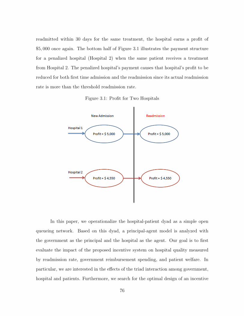
readmitted within 30 days for the same treatment, the hospital earns a profit of
$5, 000 once again. The bottom half of Figure 3.1 illustrates the payment structure
for a penalized hospital (Hospital 2) when the same patient receives a treatment
from Hospital 2. The penalized hospital’s payment causes that hospital’s profit to be
reduced for both first time admission and the readmission since its actual readmission
rate is more than the threshold readmission rate.
Figure 3.1: Profit for Two Hospitals
In this paper, we operationalize the hospital-patient dyad as a simple open
queueing network. Based on this dyad, a principal-agent model is analyzed with
the government as the principal and the hospital as the agent. Our goal is to first
evaluate the impact of the proposed incentive system on hospital quality measured
by readmission rate, government reimbursement spending, and patient welfare. In
particular, we are interested in the effects of the triad interaction among government,
hospital and patients. Furthermore, we search for the optimal design of an incentive
76

mechanism that can better save the government’s expense and improve the welfare
of the patients. As a positive alternative to the penalty-based incentive mechanism,
we extend our current framework to include the possibility and the provision of in-
centives to reduce readmission rates by enhancing hospital’s post-discharge care (e.g.
close follow-up, home care support program) as well as motivating better patients’
cooperation with the treatment procedure.
Several potential incentive issues exist in this environment. The hospital gen-
erates revenue from a patient’s discharge and is motivated to shorten the duration
of patient stay by discharging the patient earlier. Although these decisions must be
based on “objective” expertise judgment and the patient’s interest, they are indistin-
guishable from the government’s perspective. This is a typical moral hazard incentive
issue. This is essentially the reason that the penalty scheme should be risk-adjusted.
We investigate analytically whether or not the proposed PPACA plan makes the best
use of the observable information. We use a standard principal-agent moral hazard
model to examine the effects of this synergy between hospital and patients on the
design of incentive mechanisms for the hospital and the healthcare system as a whole.
This paper makes significant contributions. It provides key insights to policy
makers regarding the impact of the proposed plan to penalize hospitals with high
readmissions on the hospitals and the patient welfare. In particular, results indicate
that, depending on the price to cost ratio of the treatment, the optimal readmission
rate for hospitals will be zero or a value greater than zero but less than the threshold
value of readmission rate allowed by the government. We find that the optimal value
of hospital’s readmission rate increases as the threshold value allowed by the govern-
ment increases. Similarly, the optimal value of hospital’s readmission rate increases
as the penalty imposed by the government on hospitals with high readmissions de-
creases. As a socially responsible organization, the government needs to take into
77

account the interest of society as a whole. More specifically, the government objec-
tive is to optimize the weighted sum of hospital’s expected profit, patient welfare,
and government’s cost. These results provide timely insight to the government policy
makers about the threshold value of the allowed readmission rate, payment factor,
and patient welfare and to the hospitals about the optimal value of the readmission
rate that they should maintain to maximize their profits.
The rest of this paper is organized in the following way. We review relevant
literature in Section 3.2 and present our mathematical model in Section 3.3. We
present results and mathematical proofs in Section 3.4 and discuss the implications
of these results and conclude in Section 3.5.
3.2 Literature Review
We review two streams of literature: healthcare operations management and
principal-agent models applied to healthcare industry. First, we present a review of
the relevant healthcare literature and applications of healthcare in operations man-
agement literature. Second, we present a brief review of the papers that have used
principal-agent model and game theory in healthcare operations setting. There are
multiple operations management studies about strategic healthcare delivery decisions
such as analytical articles about capacity requirements (e.g., number of beds, staffing)
and other decisions such as scheduling surgeries. Other studies have examined how
to streamline patient flows (see Green 2004 for a detailed review and Roth et al. 1996
for a discussion on hospitals’ operations strategies). Although there have been many
analytic studies on healthcare in operations management, there have been very few
papers dealing with readmissions from an operations perspective. KC and Terwiesch
(2012) estimate the effect of initial length of stay of patients in one hospital’s intensive
78

cardiac unit on probability of readmission of the patients from step down care center
back to the ICU. They find that the initial length of stay has a negative effect on the
probability of readmission. In the light of the new penalty plan, Bartel et al. (2013)
extend this finding to the set of entire Medicare patients across all the hospitals in the
U.S. There have been two notable papers on readmissions from a policy perspective.
Friedman and Basu (2004) use proprietary cost and readmissions data of a sample of
U.S. hospitals to compute the total cost to the payer (U.S. Government or Medicare)
due to potential readmissions. Venkataraman et al. (2013) estimate the effect of read-
missions on marginal cost of hospitals using data on hospitals in Arizona. They find
that readmission rates have positive effect on marginal cost. We use this result in our
mathematical model to model the hospital cost, as described in detail in Section 3.3.
We use operations strategy theoretical lens to posit that readmission in health-
care implies quality defect (Garvin 1987). In particular, a readmission does not meet
Juran’s (1992) definition of “freedom from deficiencies”. A readmission does not al-
so meet the patient’s requirement or standard of care. So, high readmission rates
are considered to be indicators of poor quality (Rau 2011). Quality is a multidi-
mensional construct. Eight dimensions of quality (performance, features, reliability,
conformance, durability, serviceability, aesthetics, and perceived quality) have been
identified in the manufacturing sector (Garvin 1987). We believe that all these di-
mensions, except durability, also apply in the healthcare services.
Recently, Eappen, Lane, Rosenberg, Lipsitz, Sadoff, Matheson, Berry, Lester,
and Gawande (2013) published their findings on the relationship between occurrence
of surgical complications and hospital finances. Their empirical findings using data
of a Texas hospital system indicate that hospitals have financial incentives to create
surgical complications since these complications change the diagnosis related group
(DRG) of the surgery, which in turn increases the payment from the Medicare. As
79

indicated above, the effect of readmissions on financial incentives for government and
hospitals was recently examined by Friedman and Basu (2004) and Venkataraman
et al. (2013) respectively. However, the impact of the potential penalization plan,
including the threshold value allowed by the government and the penalty structure
on the optimal readmission rate and patient welfare remains yet to be analyzed. This
paper fills in this literature gap.
Principal-agent model and queueing models have been used often in the health-
care and quality operations management literature. So and Tang (2000) develop a
mathematical model to understand the effect of reimbursement policy for drugs on
the drug usage by the clinic. They find that patients with worse initial conditions
and drugs with lower profit margin will force the clinics to set a lower output target
level of the patients’ well being. They also find that the clinics will set a lower output
target level if the reimbursement threshold set by the payer for a particular drug is
lower, which is intuitive. Fuloria and Zenios (2001) develop a dynamic principal-agent
model to outline the FFS payment system of Medicare (purchaser of medical services)
and a hospital (provider), where the Medicare’s problem is to maximize the social
welfare and hospital’s problem is to maximize its expected profit. They find that the
Medicare should move to a prospective payment system with a retrospective penalty
on deaths occurring in the hospital. Our problem is similar, however, the current
system itself is of prospective payment and we do not consider linear payment system
as considered by them. Jiang et al. (2013) model pay for performance outpatient
healthcare system as a principal-agent model where the payer’s (principal) problem
is to minimize the cost while achieving a target waiting time for the patient and the
hospital’s problem is to maximize its profit given the contracting terms by the princi-
pal. The hospital dynamics are modeled as a M/D/1 queueing system. They find that
the linear contract cannot achieve the second-best solution and propose a threshold
80

penalty payment system. Chao et al. (2003) analyze customer flows between different
sites in a multisite healthcare system and provide guidelines for resource allocation
in such cases while meeting a target for waiting time of patients. Anand et al. (2011)
study customer-intensive queueing systems where quality and speed are trade-offs.
They find that customer intensity leads to results different from those of conventional
queueing systems. In particular, the speed of the servers reduces as the number of
competing servers goes up and the price charged by the server increases as the number
of competing servers goes up. We build on this stream of literature by modeling a
prospective payment system healthcare service as a principal-agent model with gov-
ernment (payer) being the principal hospital (provider) being the agent. The payer’s
problem is to maximize its expected profit, which is modeled as a weighted average
of hospital’s expected profit, patient welfare and payer’s cost, which is explained in
detail in Section 3.3.
3.3 Model
Timeline of events of admission and readmission to a hospital and the payment
details are shown in Figure 3.2 and all the notations used in the model are listed in
Table 3.1.
We assume k ∼ BIN(N, r) and since N is sufficiently large, we use normal approxima-
tion to binomial. So, k ∼ N(Nr,Nr(1− r)), and X =k −Nr√Nr(1− r)
∼ N(0, 1). The
hospital gets full payment (pN) from Medicare if its realized readmission rate (k/N)
is lower than the threshold readmission rate (α) while it gets a penalized payment
(pδN) if its realized readmission rate (k/N) is greater than the threshold readmission
rate (α).
81

Figure 3.2: Timeline
Expected Revenue = Pr
[k
N≤ α
](Exp. Rev. | k
N≤ α
)+ Pr
[k
N> α
](Exp. Rev. | k
N> α
)= Pr
[k
N≤ α
](pN + pk | k
N≤ α
)+ Pr
[k
N> α
](δpN + δpk | k
N> α
).
E[k; k ≤ Nα] = E[√Nr(1− r)X +Nr;
√Nr(1− r)X +Nr ≤ Nα]
=√Nr(1− r)E
[X;X ≤ N(α− r)√
Nr(1− r)
]
+NrE
[1;X ≤ N(α− r)√
Nr(1− r)
]
= −√Nr(1− r)
2πexp
−N
2(α− r)2
2Nr(1− r)
+NrΦ
(N(α− r)√Nr(1− r)
).
82
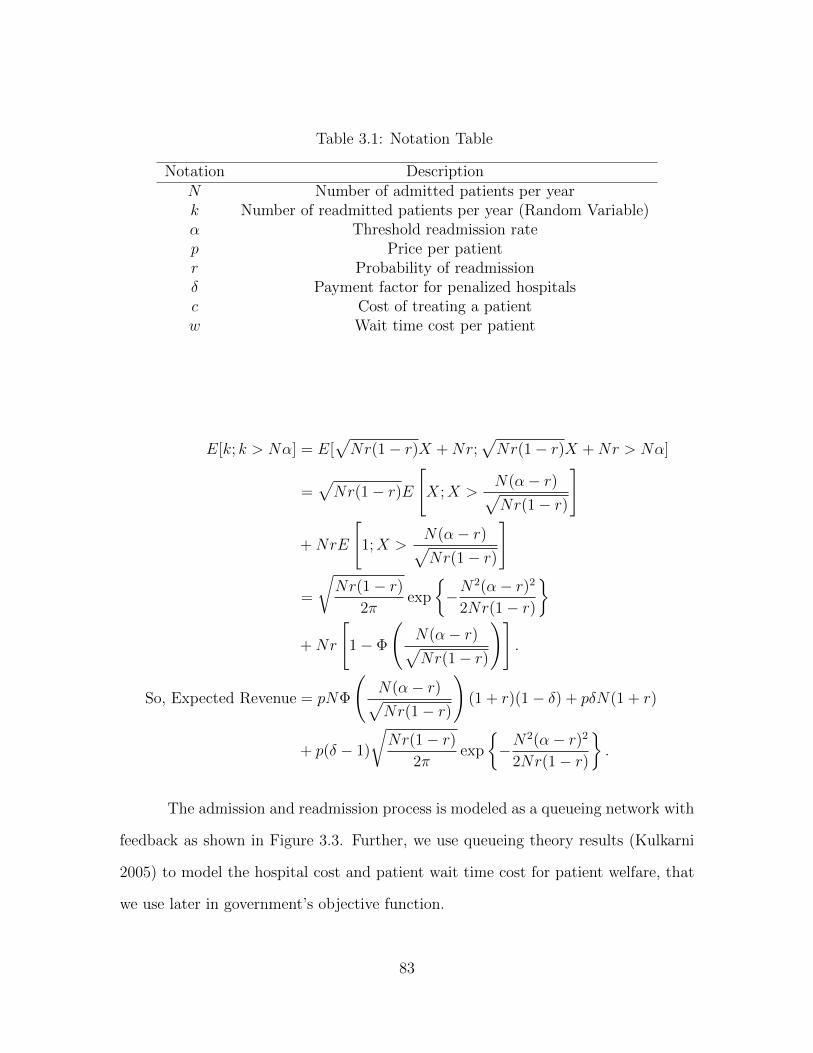
Table 3.1: Notation Table
Notation DescriptionN Number of admitted patients per yeark Number of readmitted patients per year (Random Variable)α Threshold readmission ratep Price per patientr Probability of readmissionδ Payment factor for penalized hospitalsc Cost of treating a patientw Wait time cost per patient
E[k; k > Nα] = E[√Nr(1− r)X +Nr;
√Nr(1− r)X +Nr > Nα]
=√Nr(1− r)E
[X;X >
N(α− r)√Nr(1− r)
]
+NrE
[1;X >
N(α− r)√Nr(1− r)
]
=
√Nr(1− r)
2πexp
−N
2(α− r)2
2Nr(1− r)
+Nr
[1− Φ
(N(α− r)√Nr(1− r)
)].
So, Expected Revenue = pNΦ
(N(α− r)√Nr(1− r)
)(1 + r)(1− δ) + pδN(1 + r)
+ p(δ − 1)
√Nr(1− r)
2πexp
−N
2(α− r)2
2Nr(1− r)
.
The admission and readmission process is modeled as a queueing network with
feedback as shown in Figure 3.3. Further, we use queueing theory results (Kulkarni
2005) to model the hospital cost and patient wait time cost for patient welfare, that
we use later in government’s objective function.
83

Figure 3.3: Queueing with Feedback
Time Spent by a patient in a hospital =1
(1− r)µ−N
Hospital Cost =cN
(1− r)µ−N, (3.59)
where µ is the hospital capacity. Similarly,
Patient Cost =wN
(1− r)µ−N. (3.60)
So, the hospital’s expected profit is given by the difference between its expected
revenue and cost.
Hospital Profit = pNΦ
(N(α− r)√Nr(1− r)
)(1 + r)(1− δ) + pδN(1 + r)
+ p(δ − 1)
√Nr(1− r)
2πexp
−N
2(α− r)2
2Nr(1− r)
− cN
(1− r)µ−N.
(3.61)
84

The government side problem is modeled as optimizing the weighted average
of hospital’s profit, patient welfare, and government’s cost (which is equal to the
hospital’s revenue). Using Equations 3.59 and 3.60, government’s objective is given
by
Government’s Objective = ξ [τ(Hospital Profit)− (1− τ)(Patient Cost)]
− (1− ξ)(Hospital Revenue)
= β1(Hospital Revenue) + β2(Hospital Cost)
+ β3(Patient Cost)
= β1(Hospital Profit) + β′2(Hospital Cost)
+ β3(Patient cost), (3.62)
where ξ and τ are any given weights, β1 = ξτ − 1 + ξ, β2 = −ξτ, β3 = −ξ(1− τ), β′2 =
β1 + β2 = ξ − 1.
3.4 Results
The theorems below determine the optimal value of readmission rate r∗, which
maximizes hospital’s expected profit. Proofs of all theorems are in appendix.
Theorem 1. If p <cµ
(µ−N)2, then r∗ = 0.
Theorem 1 shows that it is optimal for hospitals to have zero readmission
rate if the price to cost ratio is below a threshold value. This is intuitive since for
treatments with low price to cost ratio, hospitals will have no incentives to induce
readmissions, while for treatments with high price to cost ratio, hospitals will have
incentives to induce readmissions as shown in Theorem 2.
85

Theorem 2. If p ≥ cµ
(µ−N)2, then ∃ a r∗ < α such that
∂Π
∂rat r = r∗ is zero.
Theorem 3 proves the uniqueness of r∗.
Theorem 3. r∗ is unique if δ <cµ
p [(1− r)µ−N ]2or if
δ <(1 + r∗)
(1 + r)+
c
p(1 + r)
[1
(1− r)µ−N− 1
(1− r∗)µ−N
]∀ r > α.
To analyze the government’s objective function in Equation 3.62, we first in-
vestigate the effect of threshold readmission rate and payment factor set by the gov-
ernment on optimal readmission rate of the hospital and patient cost. We use the
numerical values given in Table 3.2.
Table 3.2: Numerical Values
Notation ValueN 10, 000p 70, 000c 60, 000w 45, 000µ 22, 000
As seen in Figure 3.4, optimal readmission rate (r∗) increases as the threshold
readmission rate (α) increases and if payment factor (δ) increases. This effect is
intuitive since as the threshold readmission rate and payment factor increase, the
government is allowing more readmissions and hence hospitals have incentive to induce
more readmissions.
We prove these results analytically in Theorems 4 and 5 respectively. Also, the
effect of threshold readmission rate is steeper than the effect of payment factor. This
implies that the government should pay more attention to setting the right threshold
readmission rate than setting the right payment factor.
86

Figure 3.4: Effect of Threshold Readmission Rate and Payment Factor on OptimalReadmission Rate
00.2
0.40.6
0.81
0
0.2
0.4
0.6
0.80
0.1
0.2
0.3
0.4
0.5
Payment Factor (δ)Threshold Readmission Rate (α)
Opt
imal
Rea
dmis
sion
Rat
e (r
* )
Theorem 4. Optimal readmission rate (r∗) is non-decreasing in threshold readmis-
sion rate (α).
Theorem 5. Optimal readmission rate (r∗) is non-decreasing in payment factor (δ).
Figure 3.5 shows the effect of threshold readmission rate and payment factor
on optimal patient cost. Since optimal patient cost increases as optimal readmission
rate increases, the effects of threshold readmission rate and payment factor on optimal
patient cost are similar to their effects on optimal readmission rate. This implies that
if government’s policy goes awry, then patient’s welfare will be adversely affected.
87

Figure 3.5: Effect of Threshold Readmission Rate and Payment Factor on OptimalPatient Cost
00.2
0.40.6
0.81
0
0.2
0.4
0.6
0.80
1
2
3
4
5
x 105
Payment Factor (δ)Threshold Readmission Rate (α)
Pat
ient
Cos
t
3.5 Conclusions
This paper examined the impact of Medicare’s plan to penalize hospitals with
readmission rates greater than the corresponding government determined threshold
readmission rates on government, hospitals, and patients. To study the impact of
the plan, a principal-agent model is developed with government as the principal and
hospital as the agent. The hospital’s problem is modeled as an optimization problem
to maximize expected profit which is the difference between expected revenue and
hospital’s cost. The hospital gets full payment if its empirical readmission rate is
less than the government set threshold readmission rate, whereas it gets a penalized
88

payment if its empirical readmission rate is greater than the threshold readmission
rate. To model hospital’s cost and patient wait time cost, queueing with feedback
model results were used. We find that hospital’s optimal readmission rate will be zero
or a value greater than zero, but less than the threshold readmission rate depending
on the ratio of price to cost of the treatment. The government’s problem is modeled to
optimize hospital’s profit and patient wait time cost (both of these together constitute
societal welfare at large) and government’s cost. We find that if government’s policy
goes wrong, then hospitals will be the main beneficiary, while the patient’s welfare will
be adversely affected. We plan to extend the government side optimization problem
by imposing the individual rationality constraint so that the hospitals participate
in this penalty plan. If not, the hospitals would prefer going bankrupt instead of
participating in this program.
This paper has certain limitations. First, homogeneity of patients was as-
sumed for modeling simplicity. However, in reality patients’ characteristics are very
heterogeneous. Second, a fixed price and unit hospital cost and patient welfare cost
was assumed due to the assumption of patient homogeneity. Third, individual ra-
tionality constraint was relaxed in the current analysis. However, we plan to extend
our analysis by imposing the constraint. In spite of these limitations, the results of
this essay provide timely insights to hospital administrators and policy makers in the
government as well as the patients in light of the recent Medicare penalty.
This essay provides several avenues for future research. First, a dynamic
principal-agent model can be built to find the hospital’s optimal decision over a period
of time given the penalty, threshold readmission rate in each time period and hospi-
tal’s decision in the previous periods. Second, patient’s heterogeneity can be modeled
which will be private information to hospitals only. Third, after the data for payment
factor, threshold readmission rate and realized readmission rate become available; an
89

empirical analysis could be done to study the impact of penalty on readmission rate
of all hospitals in the U.S.
90

Conclusions
First, this dissertation finds key antecedents that affect efficiency in bank-
ing industry and effectiveness in healthcare industry. Although efficiency in banking
industry has been estimated many times in the past, test of equality of means com-
paring efficiency of two groups in banking industry has been missing in the literature.
The first essay of this dissertation fills this gap by testing equality of means of banks
operating in the U.S. and in India. The hypothesis is grounded in diffusion theory,
where by technology diffusion has enabled banks operating in India to catch up with
their western counterparts in terms of efficient banking, especially after foreign banks
were allowed to operate in India since 1990. The second hypothesis of the first essay,
grounded in path dependence theory, contrasts the means of state-owned banks, do-
mestic private banks, and foreign banks operating in India. We find evidence of path
dependence, i.e., the economic policies until 1990 that gave inherent advantage to the
state-owned banks still have an effect in India and hence we find that state-owned
banks are more efficient than domestic private and foreign banks in India. This im-
plies that the Indian government needs to carry forward the liberalization policies
further to enable efficient operation of domestic private and foreign banks. By in-
terviewing managers of all three type of banks in India, we found that state-owned
banks tend to hire “better” employees by having a nation-wide test and an interview
91

process. Domestic private and foreign banks in India need to manage their labor in
a more efficient way through better in-house training programs. They should also
pursue innovation which will enable them to be more efficient and in turn will help
them in making investments. This would mean that domestic private and foreign
banks should probably focus on innovation to compensate for the path dependence
disadvantage. These banks should also manage their labor better. The foreign banks
have recently been able to attract employees by paying higher salary and hence future
research on this topic after a decade will probably show that the domestic private
and foreign banks are equally or more efficient than state-owned banks.
Second, this dissertation finds cost drivers of hospitals in healthcare industry.
The second essay finds that readmission rate increases marginal cost of the hospital,
defined as the cost of treating one patient per episode, significantly. In particular, we
find that as the readmission rate increases by 1 percent, the marginal cost incurred by
the hospital goes up by 7.2 percent. This finding is very significant since this increase
coupled with the recent act (PPACA) to penalize hospitals with high readmission
rates will serve as “double whammy” to the hospitals. Interestingly, the local hospi-
tal administrators who we talked to are not aware of this effect in their hospital and
hence this finding has the potential to be impactful in the light of Medicare’s recent
penalization plan. This finding has a operations strategy quality management impli-
cation. Readmissions are costly for hospitals and hence hospitals should invest more
in quality failure prevention costs (Juran 1992). The second essay of this dissertation
also estimates the impact of the potential penalty on the average readmission rate
of all hospitals in three markets in the state of Arizona. We find that the market in
which initial competition among hospitals in terms of their readmission rates is high
achieves lower average readmission rate in the steady-state once the penalty sets in.
We also find that with the introduction of stochastic shock, the hospitals in market
92

with low competition tend to achieve lower readmission rate than without stochastic
shock. However, this effect is reverse in the market with high competition in terms of
their initial readmission rate. After eliminating critical access hospitals, we find that
the average price charged by the acute care hospitals remains the same. This implies
that the patient welfare in terms of their cost will remain unaffected even if critical
access hospitals go out of business. However, their access to care will be severely
affected and hence we do not recommend elimination of critical access hospitals.
The third essay of this dissertation builds on the second essay by developing
a principal-agent model to analyze the impact of PPACA on government, hospitals,
and patients. The hospital side problem is modeled as maximization of its expected
profit which is the difference between its expected revenue from the government and
its cost. The hospital will get full revenue if its realized readmission rate (number
of readmissions/total admissions) is less than the government determined threshold
readmission rate, while it will get a penalized payment if its realized readmission
rate is higher than the threshold readmission rate. We find that the optimal value
of readmission rate that maximizes hospital’s expected profit is zero or an interior
value greater than zero but less than the threshold readmission rate depending on the
price to cost ratio of the treatment. The government side is modeled as an optimiza-
tion problem with weights for hospital profit, patient welfare, and government cost.
Analytical and numerical results indicate that if the government gives low weight to
hospital profit and societal welfare in general, then the optimal threshold readmission
rate and the optimal payment factor that optimizes government objective are their
lower bounds respectively. However, if the government gives high weight to hospital
profit and societal welfare in general, then the optimal threshold readmission rate and
payment factor is greater than zero but less than the respective upper bounds. Re-
sults also indicate that optimal readmission rate and patient cost are non-decreasing
93

in threshold readmission rate and payment factor set by the government.
This dissertation makes several contributions to the service and healthcare op-
erations management literature. First, it integrates diffusion theory from marketing
and path dependence theory from economics in to service operations. Second, it in-
troduces test of convexity and test of equality of means to the operations management
literature when estimating efficiency of decision making units. Third, this dissertation
provides hospital administrators an internal incentive to reduce readmission rates on
their own even without the Medicare plan to penalize hospitals with high readmis-
sion rates. Fourth, the findings of the second essay provide an alignment of goals
between the government that actively seeks to reduce readmission rates and the hos-
pitals, which now have an internal incentive to reduce readmission rates. Fifth, the
structural estimation methodology can be used by policy makers to estimate hospital
cost especially in the case of proprietary hospitals, which are not obligated to publish
their cost data. Sixth, our findings from the third essay provide valuable insights to
the government, hospitals, and the patients in light of the Medicare’s penalty plan.
94

Appendices
95

Appendix A Proofs of Theorems in Essay 3
Proof of Theorem 1
Proof.
∂Π
∂r= pδN +
pN(δ − 1)(1− 2r)
4π
exp(−N(α−r)2
2r(1−r)
)√
Nr(1−r)2π
+ pN(δ − 1)
√Nr(1− r)
2πexp
(−N(α− r)2
2r(1− r)
)[α− rr(1− r)
+(α− r)2
2r2(1− r)− (α− r)2
2r(1− r)2
]+ pN(1− δ)Φ
(N(α− r)√Nr(1− r)
)
+ pN(1 + r)(δ − 1) exp
(−N(α− r)2
2r(1− r)
)√N
2πr(1− r)
+pN(1 + r)(δ − 1) exp
(−N(α−r)2
2r(1−r)
)2√
2π
N2(α− r)(1− 2r)√[Nr(1− r)]3
− cNµ
[(1− r)µ−N ]2.
When r = 0
∂Π
∂r= pδN + pN(1− δ)− cNµ
(µ−N)2
= N
[p− cµ
(µ−N)2
].
So,∂Π
∂rat r = 0 is ≥ 0 if and only if
p ≥ cµ
(µ−N)2. (63)
96

If Equation 63 does not hold, for any r (r 6≈ α)
∂Π
∂r= pδN + pN(1− δ)Φ
(N(α− r)√Nr(1− r)
)− cNµ
((1− r)µ−N)2
≤ pδN + pN(1− δ)− cNµ
((1− r)µ−N)2
= N
[p− cµ
((1− r)µ−N)2
]≤ N
[p− cµ
(µ−N)2
]< 0.
So, r∗ = 0.
Proof of Theorem 2
Proof. Assuming Equation 63 holds, when r = α,
∂π
∂r= pδN +
pN(δ − 1)
4π
(1− 2α)√Nα(1−α)
2π
+pN(1− δ)
2+ pN(1 + α)(δ − 1)
√N
2πα(1− α)
− cNµ
[(1− α)µ−N ]2
= pN
[0.5 +
δ
2+ (δ − 1)
((1− 2α)
4π
√2π
Nα(1− α)+
√N(1− α)
2πα
)]
− cNµ
[(1− α)µ−N ]2
So,∂π
∂rat r = α is < 0 if and only if
δ <
cµ[(1−α)µ−N ]2
p[
(1−2α)4π
√2π
Nα(1−α)+√
N(1+α)2
2πα(1−α)+ 1
2
] +p[
(1−2α)4π
√2π
Nα(1−α)+√
N(1+α)2
2πα(1−α)− 1
2
]p[
(1−2α)4π
√2π
Nα(1−α)+√
N(1+α)2
2πα(1−α)+ 1
2
] .(64)
The second term of Equation 64 is close to 1 for largeN . So, the above equation
always holds for large N since δ < 1. So,∂π
∂rat r = α is < 0. By intermediate value
97

theorem, there exists a r∗ < α such that∂π
∂rat r = r∗ is 0.
Proof of Theorem 3
Proof. For r > α (r 6≈ α):
∂π
∂r= pδN − cNµ
((1− r)µ−N)2
= N
[pδ − cµ
((1− r)µ−N)2
].
So,∂π
∂r< 0 if and only if
cµ
((1− r)µ−N)2> pδ. (65)
If the condition in Equation 65, then uniqueness is proved. If the condition
does not hold true, then we need to show that E[Π] at r = r∗ < α is greater than
E[Π] at any r > α.
E[Π]r∗ = pδN(1 + r∗) + pN(1 + r∗)(1− δ)− cN
[(1− r∗)µ−N ], (66)
and at any r > α (r is not close to α):
E[Π] = pδN(1 + r)− cN
[(1− r)µ−N ]. (67)
So, E[Π]r∗ > E[Π] at any r > α if and only if
pδN(1 + r∗) + pN(1 + r∗)(1− δ)− cN
[(1− r∗)µ−N ]> pδN(1 + r)− cN
[(1− r)µ−N ]
pδr∗ + p(1 + r∗)(1− δ)− c
[(1− r∗)µ−N ]> pδr − c
[(1− r)µ−N ]
98

or
δ <(1 + r∗)
(1 + r)+
c
p(1 + r)
[1
(1− r)µ−N− 1
(1− r∗)µ−N
].
The last condition should hold for all values for r > α. Note: the first term on the
RHS of last equation is strictly less than 1 and the second term is strictly greater
than 0.
Proof of Theorem 4
99

Proof.
∂(Hospital Profit)
∂r∗∂α=p(1− δ)N2(α− r∗)(1− 2r∗) exp
(−N(α−r∗)2
2r∗(1−r∗)
)2r∗(1− r∗)
√2πNr∗(1− r∗)
− pN3(1 + r∗)(1− δ)(1− 2r∗)
2√
2π [Nr∗(1− r∗)]3
+p(1− δ)N2 exp
(−N(α−r∗)2
2r∗(1−r∗)
)√
2πNr∗(1− r∗)
−p(1− δ)N exp
(−N(α−r∗)2
2r∗(1−r∗)
)√Nr∗(1− r∗)2π
r∗(1− r∗)
+p(1− δ)N2(α− r∗)2
[r∗(1− r∗)]2
√Nr∗(1− r∗)
2πexp
(−N(α− r∗)2
2r∗(1− r∗)
)+p(1− δ)N2(α− r∗)3
2r∗3(1− r∗)2
√Nr∗(1− r∗)
2πexp
(−N(α− r∗)2
2r∗(1− r∗)
)− p(1− δ)N2(α− r∗)3
2r∗2(1− r∗)3
√Nr∗(1− r∗)
2πexp
(−N(α− r∗)2
2r∗(1− r∗)
)
−p(1− δ)N(α− r∗) exp
(−N(α−r∗)2
2r∗(1−r∗)
)√Nr∗(1− r∗)2π
r∗2(1− r∗)
+p(1− δ)N(α− r∗) exp
(−N(α−r∗)2
2r∗(1−r∗)
)√Nr∗(1− r∗)2π
r∗(1− r∗)2
+pN3(1 + r∗)(1− δ)(α− r∗) exp
(−N(α−r∗)2
2r∗(1−r∗)
)r∗(1− r∗)
√2πNr∗(1− r∗)
+pN3(1 + r∗)(1− δ)(α− r∗)2 exp
(−N(α−r∗)2
2r∗(1−r∗)
)2r∗2(1− r∗)
√2πNr∗(1− r∗)
−pN3(1 + r∗)(1− δ)(α− r∗)2 exp
(−N(α−r∗)2
2r∗(1−r∗)
)2r∗(1− r∗)2
√2πNr∗(1− r∗)
100

∂(Hospital Profit)
∂r∗∂α≥ 0 since
N(α− r∗)(1 + r∗)
√N
2πr∗(1− r∗)≥ (1 + r∗)(1− 2r∗)
√N
8πr∗(1− r∗)
and
N(α− r∗)2
√N
2πr∗(1− r∗)≥ (α− r∗)
√N(1− r∗)
2πr∗.
Proof of Theorem 5 is similar to the proof Theorem 4.
101

Appendix B Codes of Computer Programs
Codes of computer programs for all essays are presented in this appendix.
B.1 Essay 1
All the codes for Essay 1 are written in “R” software
Sample Code for Detecting Outliers using Wilson (1993) Method
(“C:/Users/Sriram/Desktop/Summer Paper”)
comb=read.csv(“combined deposits investments.csv”)
n=nrow(comb)
x=t(matrix(c(comb$Deposits,comb$Employees),nrow=n,ncol=2))
y=t(matrix(c(comb$Loans,comb$Investments),nrow=n,ncol=2))
outlier1=ap(x,y,NDEL=12)
Detecting Outliers using Simar (2003) Method
setwd(“C:/Users/Sriram/Downloads/Summer Paper”)
t=read.csv(“outliers loo us indian.csv”)
n=nrow(t)
k=n-1
dhat=matrix(nrow=198,ncol=1)
for (i in 1:198)
t1=t[i,]
tref=t[-i,]
x1=t(matrix(c(t1$Deposits,t1$Employees),nrow=1,ncol=2))
y1=t(matrix(c(t1$Loans,t1$Investments),nrow=1,ncol=2))
102

xre=t(matrix(c(tref$Deposits,tref$Employees),nrow=k,ncol=2))
yre=t(matrix(c(tref$Loans,tref$Investments),nrow=k,ncol=2))
dhat[i,1]=dea(XOBS=x1,YOBS=y1,XREF=xre,YREF=yre)
write.csv(dhat,“outliers loo us indian eff.csv”)
Testing Convexity of Production Frontier
setwd(“C:/Users/Sriram/Downloads/Summer Paper”)
t=read.csv(“combined deposits investments 4 loans employees loo us indian.csv”)
n = nrow(t)
X = t(matrix(c(t$Deposits, t$Employees), nrow = n, ncol = 2))
Y = t(matrix(c(t$Loans, t$Investments), nrow = n, ncol = 2))
p=2
q=2
a=2*(p+q)/(p+q+1)
k=seq(1,(n-1),1)
k=k[which.min(abs(n-k-k**a))]
m=n-k
ind=sample.int(n,size=k,replace=FALSE)
X1=X[,ind]
Y1=Y[,ind]
X2=X[,-ind]
Y2=Y[,-ind]
ghat1=dea(XOBS = X1, YOBS = Y1)
ghat2=fdh(XOBS = X2, YOBS = Y2)
ghat2=t(ghat2)
103

k1=floor(k/2)
ind1=sample.int(k,size=k1,replace=FALSE)
X11=X1[,ind1]
Y11=Y1[,ind1]
X12=X1[,-ind1]
Y12=Y1[,-ind1]
ghat11=dea(XOBS = X11, YOBS = Y11)
ghat12=dea(XOBS = X12, YOBS = Y12)
m1=floor(m/2)
ind2=sample.int(m,size=m1,replace=FALSE)
X21=X2[,ind2]
Y21=Y2[,ind2]
X22=X2[,-ind2]
Y22=Y2[,-ind2]
ghat21=fdh(XOBS = X21, YOBS = Y21)
ghat21=t(ghat21)
ghat22=fdh(XOBS = X22, YOBS = Y22)
ghat22=t(ghat22)
kappa2=1/(p+q)
n1mean=floor(k**(2*kappa2))
n2mean=floor(m**(2*kappa2))
indmean1=sample.int(k,size=n1mean,replace=FALSE)
indmean2=sample.int(m,size=n2mean,replace=FALSE)
X1mean=X1[,indmean1]
Y1mean=Y1[,indmean1]
X2mean=X2[,indmean2]
104

Y2mean=Y2[,indmean2]
ghatmean1=dea(XOBS = X1mean, YOBS = Y1mean,XREF=X1,YREF=Y1)
ghatmean2=fdh(XOBS = X2mean, YOBS = Y2mean,XREF=X2,YREF=Y2)
ghatmean2=t(ghatmean2)
write.csv(ghat1,“DEA1 eff.csv”)
write.csv(ghat2,FDH2 eff.csv”)
write.csv(ghat11,“DEA11 eff.csv”)
write.csv(ghat12,“DEA12 eff.csv”)
write.csv(ghat21,“FDH21 eff.csv”)
write.csv(ghat22,“FDH22 eff.csv”)
write.csv(ghatmean1,“DEAmean1 eff.csv”)
write.csv(ghatmean2,“FDHmean2 eff.csv”)
Estimating Efficiency using FDH Estimator
setwd(“C:/Users/Sriram/Downloads/Summer Paper”)
t=read.csv(“combined deposits investments 4 loans employees loo us indian.csv”)
n=nrow(t)
x=t(matrix(c(t$Deposits,t$Employees),nrow=n,ncol=2))
y=t(matrix(c(t$Loans,t$Investments),nrow=n,ncol=2))
dhat=fdh(XOBS=x,YOBS=y)
write.csv(dhat,“all deposits investments 4 loans employees loo us indian fdh.csv”)
Testing Hypothesis 1
setwd(“C:/Users/Sriram/Downloads/Summer Paper/hypothesis1”)
t1=read.csv(“usbanks.csv”)
n1 = nrow(t1)
105

X1 = t(matrix(c(t1$Deposits, t1$Employees), nrow = n1, ncol = 2))
Y1 = t(matrix(c(t1$Loans, t1$Investments), nrow = n1, ncol = 2))
ghat1=fdh(XOBS = X1, YOBS = Y1)
ghat1=t(ghat1)
k1=floor(n1/2)
ind1=sample.int(n1,size=k1,replace=FALSE)
X11=X1[,ind1]
Y11=Y1[,ind1]
X12=X1[,-ind1]
Y12=Y1[,-ind1]
ghat11=fdh(XOBS = X11, YOBS = Y11)
ghat11=t(ghat11)
ghat12=fdh(XOBS = X12, YOBS = Y12)
ghat12=t(ghat12)
t2=read.csv(“indianbanks.csv”)
n2 = nrow(t2)
X2 = t(matrix(c(t2Deposits, t2Employees), nrow = n2, ncol = 2))
Y2 = t(matrix(c(t2Loans, t2Investments), nrow = n2, ncol = 2))
ghat2=fdh(XOBS = X2, YOBS = Y2)
ghat2=t(ghat2)
k2=floor(n2/2)
ind2=sample.int(n2,size=k2,replace=FALSE)
X21=X2[,ind2]
Y21=Y2[,ind2]
X22=X2[,-ind2]
Y22=Y2[,-ind2]
106

ghat21=fdh(XOBS = X21, YOBS = Y21)
ghat21=t(ghat21)
ghat22=fdh(XOBS = X22, YOBS = Y22)
ghat22=t(ghat22)
p=2
q=2
kappa=1/(p+q)
n1mean=floor(n1**(2*kappa))
n2mean=floor(n2**(2*kappa))
indmean1=sample.int(n1,size=n1mean,replace=FALSE)
indmean2=sample.int(n2,size=n2mean,replace=FALSE)
X1mean=X1[,indmean1]
Y1mean=Y1[,indmean1]
X2mean=X2[,indmean2]
Y2mean=Y2[,indmean2]
ghatmean1=fdh(XOBS = X1mean, YOBS = Y1mean,XREF=X1,YREF=Y1)
ghatmean1=t(ghatmean1)
ghatmean2=fdh(XOBS = X2mean, YOBS = Y2mean,XREF=X2,YREF=Y2)
ghatmean2=t(ghatmean2)
write.csv(ghat1,“usbanks eff fdh.csv”)
write.csv(ghat2,“indianbanks eff fdh.csv”)
write.csv(ghat11,“usbanks11 eff fdh.csv”)
write.csv(ghat12,“usbanks12 eff fdh.csv”)
write.csv(ghat21,“indianbanks21 eff fdh.csv”)
write.csv(ghat22,“indianbanks22 eff fdh.csv”)
write.csv(ghatmean1,“usbanks eff fdh mean.csv”)
107

write.csv(ghatmean2,“indianbanks eff fdh mean.csv”)
Testing Hypothesis 2a
setwd(“C:/Users/Sriram/Downloads/Summer Paper/hypothesis2a”)
t1=read.csv(“publicbanks.csv”)
n1 = nrow(t1)
X1 = t(matrix(c(t1$Deposits, t1$Employees), nrow = n1, ncol = 2))
Y1 = t(matrix(c(t1$Loans, t1$Investments), nrow = n1, ncol = 2))
ghat1=fdh(XOBS = X1, YOBS = Y1)
ghat1=t(ghat1)
k1=floor(n1/2)
ind1=sample.int(n1,size=k1,replace=FALSE)
X11=X1[,ind1]
Y11=Y1[,ind1]
X12=X1[,-ind1]
Y12=Y1[,-ind1]
ghat11=fdh(XOBS = X11, YOBS = Y11)
ghat11=t(ghat11)
ghat12=fdh(XOBS = X12, YOBS = Y12)
ghat12=t(ghat12)
t2¡-read.csv(”privatebanks.csv”)
n2 = nrow(t2)
X2 = t(matrix(c(t2$Deposits, t2$Employees), nrow = n2, ncol = 2))
Y2 = t(matrix(c(t2$Loans, t2$Investments), nrow = n2, ncol = 2))
ghat2=fdh(XOBS = X2, YOBS = Y2)
ghat2=t(ghat2)
108

k2=floor(n2/2)
ind2=sample.int(n2,size=k2,replace=FALSE)
X21=X2[,ind2]
Y21=Y2[,ind2]
X22=X2[,-ind2]
Y22=Y2[,-ind2]
ghat21=fdh(XOBS = X21, YOBS = Y21)
ghat21=t(ghat21)
ghat22=fdh(XOBS = X22, YOBS = Y22)
ghat22=t(ghat22)
p=2
q=2
kappa=1/(p+q)
n1mean=floor(n1**(2*kappa))
n2mean=floor(n2**(2*kappa))
indmean1=sample.int(n1,size=n1mean,replace=FALSE)
indmean2=sample.int(n2,size=n2mean,replace=FALSE)
X1mean=X1[,indmean1]
Y1mean=Y1[,indmean1]
X2mean=X2[,indmean2]
Y2mean=Y2[,indmean2]
ghatmean1=fdh(XOBS = X1mean, YOBS = Y1mean,XREF=X1,YREF=Y1)
ghatmean1=t(ghatmean1)
ghatmean2=fdh(XOBS = X2mean, YOBS = Y2mean,XREF=X2,YREF=Y2)
ghatmean2=t(ghatmean2)
write.csv(ghat1,“publicbanks eff fdh.csv”)
109
write.csv(ghat2,“privatebanks eff fdh.csv”)
write.csv(ghat11,“publicbanks11 eff fdh.csv”)
write.csv(ghat12,“publicbanks12 eff fdh.csv”)
write.csv(ghat21,“privatebanks21 eff fdh.csv”)
write.csv(ghat22,“privatebanks22 eff fdh.csv”)
write.csv(ghatmean1,“publicbanks eff fdh mean.csv”)
write.csv(ghatmean2,“privatebanks eff fdh mean.csv”)
Kolmogorov Smirnov Test–Hypothesis 2a
setwd(“C:/Users/Sriram/Downloads/Summer Paper/hypothesis2a”)
t1=read.csv(“KSTest Public.csv”)
t2=read.csv(“KSTest Private.csv”)
x=t1$farrell public
y=t2$farrell private
ks.test(x,y,alternative=“less”)
Testing Hypothesis 2b
setwd(“C:/Users/Sriram/Downloads/Summer Paper/hypothesis2b”)
t1=read.csv(“publicbanks.csv”)
n1 = nrow(t1)
X1 = t(matrix(c(t1$Deposits, t1$Employees), nrow = n1, ncol = 2))
Y1 = t(matrix(c(t1$Loans, t1$Investments), nrow = n1, ncol = 2))
ghat1=fdh(XOBS = X1, YOBS = Y1)
ghat1=t(ghat1)
k1=floor(n1/2)
ind1=sample.int(n1,size=k1,replace=FALSE)
110
X11=X1[,ind1]
Y11=Y1[,ind1]
X12=X1[,-ind1]
Y12=Y1[,-ind1]
ghat11=fdh(XOBS = X11, YOBS = Y11)
ghat11=t(ghat11)
ghat12=fdh(XOBS = X12, YOBS = Y12)
ghat12=t(ghat12)
t2=read.csv(“foreignbanks.csv”)
n2 = nrow(t2)
X2 = t(matrix(c(t2$Deposits, t2$Employees), nrow = n2, ncol = 2))
Y2 = t(matrix(c(t2$Loans, t2$Investments), nrow = n2, ncol = 2))
ghat2=fdh(XOBS = X2, YOBS = Y2)
ghat2=t(ghat2)
k2=floor(n2/2)
ind2=sample.int(n2,size=k2,replace=FALSE)
X21=X2[,ind2]
Y21=Y2[,ind2]
X22=X2[,-ind2]
Y22=Y2[,-ind2]
ghat21=fdh(XOBS = X21, YOBS = Y21)
ghat21=t(ghat21)
ghat22=fdh(XOBS = X22, YOBS = Y22)
ghat22=t(ghat22)
p=2
q=2
111
kappa=1/(p+q)
n1mean=floor(n1**(2*kappa))
n2mean=floor(n2**(2*kappa))
indmean1=sample.int(n1,size=n1mean,replace=FALSE)
indmean2=sample.int(n2,size=n2mean,replace=FALSE)
X1mean=X1[,indmean1]
Y1mean=Y1[,indmean1]
X2mean=X2[,indmean2]
Y2mean=Y2[,indmean2]
ghatmean1=fdh(XOBS = X1mean, YOBS = Y1mean,XREF=X1,YREF=Y1)
ghatmean1=t(ghatmean1)
ghatmean2=fdh(XOBS = X2mean, YOBS = Y2mean,XREF=X2,YREF=Y2)
ghatmean2=t(ghatmean2)
write.csv(ghat1,“publicbanks eff fdh.csv”)
write.csv(ghat2,“foreignbanks eff fdh.csv”)
write.csv(ghat11,“publicbanks11 eff fdh.csv”)
write.csv(ghat12,“publicbanks12 eff fdh.csv”)
write.csv(ghat21,“foreignbanks21 eff fdh.csv”)
write.csv(ghat22,“foreignbanks22 eff fdh.csv”)
write.csv(ghatmean1,“publicbanks eff fdh mean.csv”)
write.csv(ghatmean2,“foreignbanks eff fdh mean.csv”)
Kolmogorov Smirnov Test–Hypothesis 2a
setwd(“C:/Users/Sriram/Downloads/Summer Paper/hypothesis2b”)
t1=read.csv(“KSTest Public.csv”)
t2=read.csv(“KSTest Foreign.csv”)
112

x=t1$farrell public
y=t2$farrell foreign
ks.test(x,y,alternative=“less”)
B.2 Essay 2
B.2.1 Demand-Side Estimation
Codes for Demand-Side Estimation (using Stata software) are presented below.
xi:regress dv price totalavailablebeds i.hownercode i.eservcode i.trauma (Table 2.2)
xi:ivregress 2sls dv (price= ivbeds ivnurse ivhowner) totalavailablebeds i.hownercode
i.eservcode i.trauma (Table 2.3)
xi:regress dv price nemktsh totalavailablebeds i.hownercode i.eservcode i.trauma (Ta-
ble 2.5)
xi:ivregress 2sls dv (price nemktsh= ivnebeds ivnenurse ivneowner) totalavailablebeds
i.hownercode i.eservcode i.trauma (Table 2.6)
B.2.2 Marginal Cost Computation
Codes for marginal cost computation (using Matlab software) are presented below.
Non-Nested Model:
alpha=-0.0000941;
N=size(data,1);
for i=1:N
for j=1:N
if j==i
omega(i,j)=(alpha*data(i,27)*(1-data(i,27)));
else
113
omega(i,j)=0;
end
end
end
omega(15,16)=-alpha*data(15,27)*data(16,27);
omega(16,15)=-alpha*data(16,27)*data(15,27);
omega(23,24)=-alpha*data(23,27)*data(24,27);
omega(23,25)=-alpha*data(23,27)*data(25,27);
omega(24,23)=-alpha*data(24,27)*data(23,27);
omega(24,25)=-alpha*data(24,27)*data(25,27);
omega(25,23)=-alpha*data(25,27)*data(23,27);
omega(25,24)=-alpha*data(25,27)*data(24,27);
omega(31,32)=-alpha*data(31,27)*data(32,27);
omega(32,31)=-alpha*data(32,27)*data(31,27);
omega(57,58)=-alpha*data(57,27)*data(58,27);
omega(58,57)=-alpha*data(58,27)*data(57,27);
omega(74,75)=-alpha*data(74,27)*data(75,27);
omega(75,74)=-alpha*data(75,27)*data(74,27);
omega(82,83)=-alpha*data(82,27)*data(83,27);
omega(82,84)=-alpha*data(82,27)*data(84,27);
omega(83,82)=-alpha*data(83,27)*data(82,27);
omega(83,84)=-alpha*data(83,27)*data(84,27);
omega(84,82)=-alpha*data(84,27)*data(82,27);
omega(84,83)=-alpha*data(84,27)*data(83,27);
omega(90,91)=-alpha*data(90,27)*data(91,27);
omega(91,90)=-alpha*data(91,27)*data(90,27);
114

omega(116,117)=-alpha*data(116,27)*data(117,27);
omega(117,116)=-alpha*data(117,27)*data(116,27);
omega(133,134)=-alpha*data(133,27)*data(134,27);
omega(134,133)=-alpha*data(134,27)*data(133,27);
omega(141,142)=-alpha*data(141,27)*data(142,27);
omega(141,143)=-alpha*data(141,27)*data(143,27);
omega(142,141)=-alpha*data(142,27)*data(141,27);
omega(142,143)=-alpha*data(142,27)*data(143,27);
omega(143,141)=-alpha*data(143,27)*data(141,27);
omega(143,142)=-alpha*data(143,27)*data(142,27);
omega(149,150)=-alpha*data(149,27)*data(150,27);
omega(149,151)=-alpha*data(149,27)*data(151,27);
omega(150,149)=-alpha*data(150,27)*data(149,27);
omega(150,151)=-alpha*data(150,27)*data(151,27);
omega(151,149)=-alpha*data(151,27)*data(149,27);
omega(151,150)=-alpha*data(151,27)*data(150,27);
omega(177,178)=-alpha*data(177,27)*data(178,27);
omega(178,177)=-alpha*data(178,27)*data(177,27);
for k=5:13
for l=5:13
if l =k
omega(k,l)=-alpha*data(k,27)*data(l,27);
end
end
end
for m=64:72
115

for n=64:72
if n =m
omega(m,n)=-alpha*data(m,27)*data(n,27);
end
end
end
for p=123:131
for q=123:131
if q =p
omega(p,q)=-alpha*data(p,27)*data(q,27);
end
end
end
D=data(1:N,27);
price=data(1:N,26);
oinv=inv(omega);
mcost=price+(oinv*D);
Nested Model:
alpha=-0.0000442;
sigma=0.3569454;
N=size(d,1);
for i=1:N
for j=1:N
if j==i
o(i,j)=(alpha*d(i,27)*((1/(1-sigma)) - ((sigma*d(i,31))/(1-sigma))))
116

- (alpha*d(i,27)*d(i,27));
else
o(i,j)=0;
end
end
end
o(15,16)=-alpha*d(15,27)*((sigma*d(16,31)/(1-sigma)) + d(16,27));
o(16,15)=-alpha*d(16,27)*((sigma*d(15,31)/(1-sigma)) + d(15,27));
o(23,24)=-alpha*d(23,27)*((sigma*d(24,31)/(1-sigma)) + d(24,27));
o(23,25)=-alpha*d(23,27)*((sigma*d(25,31)/(1-sigma)) + d(25,27));
o(24,23)=-alpha*d(24,27)*((sigma*d(23,31)/(1-sigma)) + d(23,27));
o(24,25)=-alpha*d(24,27)*((sigma*d(25,31)/(1-sigma)) + d(25,27));
o(25,23)=-alpha*d(25,27)*((sigma*d(23,31)/(1-sigma)) + d(23,27));
o(25,24)=-alpha*d(25,27)*((sigma*d(24,31)/(1-sigma)) + d(24,27));
o(31,32)=-alpha*d(31,27)*((sigma*d(32,31)/(1-sigma)) + d(32,27));
o(32,31)=-alpha*d(32,27)*((sigma*d(31,31)/(1-sigma)) + d(31,27));
o(57,58)=-alpha*d(57,27)*((sigma*d(58,31)/(1-sigma)) + d(58,27));
o(58,57)=-alpha*d(58,27)*((sigma*d(57,31)/(1-sigma)) + d(57,27));
o(74,75)=-alpha*d(74,27)*((sigma*d(75,31)/(1-sigma)) + d(75,27));
o(75,74)=-alpha*d(75,27)*((sigma*d(74,31)/(1-sigma)) + d(74,27));
o(82,83)=-alpha*d(82,27)*((sigma*d(83,31)/(1-sigma)) + d(83,27));
o(82,84)=-alpha*d(82,27)*((sigma*d(84,31)/(1-sigma)) + d(84,27));
o(83,82)=-alpha*d(83,27)*((sigma*d(82,31)/(1-sigma)) + d(82,27));
o(83,84)=-alpha*d(83,27)*((sigma*d(84,31)/(1-sigma)) + d(84,27));
o(84,82)=-alpha*d(84,27)*((sigma*d(82,31)/(1-sigma)) + d(82,27));
o(84,83)=-alpha*d(84,27)*((sigma*d(83,31)/(1-sigma)) + d(83,27));
117

o(90,91)=-alpha*d(90,27)*((sigma*d(91,31)/(1-sigma)) + d(91,27));
o(91,90)=-alpha*d(91,27)*((sigma*d(90,31)/(1-sigma)) + d(90,27));
o(116,117)=-alpha*d(116,27)*((sigma*d(117,31)/(1-sigma)) + d(117,27));
o(117,116)=-alpha*d(117,27)*((sigma*d(116,31)/(1-sigma)) + d(116,27));
o(133,134)=-alpha*d(133,27)*((sigma*d(134,31)/(1-sigma)) + d(134,27));
o(134,133)=-alpha*d(134,27)*((sigma*d(133,31)/(1-sigma)) + d(133,27));
o(141,142)=-alpha*d(141,27)*((sigma*d(142,31)/(1-sigma)) + d(142,27));
o(141,143)=-alpha*d(141,27)*((sigma*d(143,31)/(1-sigma)) + d(143,27));
o(142,141)=-alpha*d(142,27)*((sigma*d(141,31)/(1-sigma)) + d(141,27));
o(142,143)=-alpha*d(142,27)*((sigma*d(143,31)/(1-sigma)) + d(143,27));
o(143,141)=-alpha*d(143,27)*((sigma*d(141,31)/(1-sigma)) + d(141,27));
o(143,142)=-alpha*d(143,27)*((sigma*d(142,31)/(1-sigma)) + d(142,27));
o(149,150)=-alpha*d(149,27)*((sigma*d(150,31)/(1-sigma)) + d(150,27));
o(149,151)=-alpha*d(149,27)*((sigma*d(151,31)/(1-sigma)) + d(151,27));
o(150,149)=-alpha*d(150,27)*((sigma*d(149,31)/(1-sigma)) + d(149,27));
o(150,151)=-alpha*d(150,27)*((sigma*d(151,31)/(1-sigma)) + d(151,27));
o(151,149)=-alpha*d(151,27)*((sigma*d(149,31)/(1-sigma)) + d(149,27));
o(151,150)=-alpha*d(151,27)*((sigma*d(150,31)/(1-sigma)) + d(150,27));
o(177,178)=-alpha*d(177,27)*((sigma*d(178,31)/(1-sigma)) + d(178,27));
o(178,177)=-alpha*d(178,27)*((sigma*d(177,31)/(1-sigma)) + d(177,27));
for k=5:13
for l=5:13
if l =k
o(k,l)=-alpha*d(k,27)*((sigma*d(l,31)/(1-sigma)) + d(l,27));
end
end
118

end
for m=64:72
for n=64:72
if n =m
o(m,n)=-alpha*d(m,27)*((sigma*d(n,31)/(1-sigma)) + d(n,27));
end
end
end
for p=123:131
for q=123:131
if q =p
o(p,q)=-alpha*d(p,27)*((sigma*d(q,31)/(1-sigma)) + d(q,27));
end
end
end
D=d(1:N,27);
price=d(1:N,26);
oinv=inv(o);
mcost=price+(oinv*D);
Nested Model: Robustness Check
alpha=-0.0000442;
sigma=0.3569454;
N=size(d,1);
for i=1:N
for j=1:N
119

if j==i
o(i,j) = (alpha*d(i,27)*((1/(1-sigma)) - ((sigma*d(i,31))/(1-sigma))))
- (alpha*d(i,27)*d(i,27));
else
o(i,j)=0;
end
end
end
o(15,16) = -alpha*d(15,27)*((sigma*d(16,31)/(1-sigma)) + d(16,27));
o(16,15) = -alpha*d(16,27)*((sigma*d(15,31)/(1-sigma)) + d(15,27));
o(23,24) = -alpha*d(23,27)*((sigma*d(24,31)/(1-sigma)) + d(24,27));
o(23,25) = -alpha*d(23,27)*((sigma*d(25,31)/(1-sigma)) + d(25,27));
o(24,23) = -alpha*d(24,27)*((sigma*d(23,31)/(1-sigma)) + d(23,27));
o(24,25) = -alpha*d(24,27)*((sigma*d(25,31)/(1-sigma)) + d(25,27));
o(25,23) = -alpha*d(25,27)*((sigma*d(23,31)/(1-sigma)) + d(23,27));
o(25,24) = -alpha*d(25,27)*((sigma*d(24,31)/(1-sigma)) + d(24,27));
o(31,32) = -alpha*d(31,27)*((sigma*d(32,31)/(1-sigma)) + d(32,27));
o(32,31) = -alpha*d(32,27)*((sigma*d(31,31)/(1-sigma)) + d(31,27));
o(57,58) = -alpha*d(57,27)*((sigma*d(58,31)/(1-sigma)) + d(58,27));
o(58,57) = -alpha*d(58,27)*((sigma*d(57,31)/(1-sigma)) + d(57,27));
o(74,75) = -alpha*d(74,27)*((sigma*d(75,31)/(1-sigma)) + d(75,27));
o(75,74) = -alpha*d(75,27)*((sigma*d(74,31)/(1-sigma)) + d(74,27));
o(82,83) = -alpha*d(82,27)*((sigma*d(83,31)/(1-sigma)) + d(83,27));
o(82,84) = -alpha*d(82,27)*((sigma*d(84,31)/(1-sigma)) + d(84,27));
o(83,82) = -alpha*d(83,27)*((sigma*d(82,31)/(1-sigma)) + d(82,27));
o(83,84) = -alpha*d(83,27)*((sigma*d(84,31)/(1-sigma)) + d(84,27));
120

o(84,82) = -alpha*d(84,27)*((sigma*d(82,31)/(1-sigma)) + d(82,27));
o(84,83) = -alpha*d(84,27)*((sigma*d(83,31)/(1-sigma)) + d(83,27));
o(90,91) = -alpha*d(90,27)*((sigma*d(91,31)/(1-sigma)) + d(91,27));
o(91,90) = -alpha*d(91,27)*((sigma*d(90,31)/(1-sigma)) + d(90,27));
o(116,117) = -alpha*d(116,27)*((sigma*d(117,31)/(1-sigma)) + d(117,27));
o(117,116) = -alpha*d(117,27)*((sigma*d(116,31)/(1-sigma)) + d(116,27));
o(133,134) = -alpha*d(133,27)*((sigma*d(134,31)/(1-sigma)) + d(134,27));
o(134,133) = -alpha*d(134,27)*((sigma*d(133,31)/(1-sigma)) + d(133,27));
o(141,142) = -alpha*d(141,27)*((sigma*d(142,31)/(1-sigma)) + d(142,27));
o(141,143) = -alpha*d(141,27)*((sigma*d(143,31)/(1-sigma)) + d(143,27));
o(142,141) = -alpha*d(142,27)*((sigma*d(141,31)/(1-sigma)) + d(141,27));
o(142,143) = -alpha*d(142,27)*((sigma*d(143,31)/(1-sigma)) + d(143,27));
o(143,141) = -alpha*d(143,27)*((sigma*d(141,31)/(1-sigma)) + d(141,27));
o(143,142) = -alpha*d(143,27)*((sigma*d(142,31)/(1-sigma)) + d(142,27));
o(149,150) = -alpha*d(149,27)*((sigma*d(150,31)/(1-sigma)) + d(150,27));
o(149,151) = -alpha*d(149,27)*((sigma*d(151,31)/(1-sigma)) + d(151,27));
o(150,149) = -alpha*d(150,27)*((sigma*d(149,31)/(1-sigma)) + d(149,27));
o(150,151) = -alpha*d(150,27)*((sigma*d(151,31)/(1-sigma)) + d(151,27));
o(151,149) = -alpha*d(151,27)*((sigma*d(149,31)/(1-sigma)) + d(149,27));
o(151,150) = -alpha*d(151,27)*((sigma*d(150,31)/(1-sigma)) + d(150,27));
o(177,178) = -alpha*d(177,27)*((sigma*d(178,31)/(1-sigma)) + d(178,27));
o(178,177) = -alpha*d(178,27)*((sigma*d(177,31)/(1-sigma)) + d(177,27));
for k=5:13
for l=5:13
if l =k
o(k,l) = -alpha*d(k,27)*((sigma*d(l,31)/(1-sigma)) + d(l,27));
121

end
end
end
for m=64:72
for n=64:72
if n =m
o(m,n) = -alpha*d(m,27)*((sigma*d(n,31)/(1-sigma)) + d(n,27));
end
end
end
for p=123:131
for q=123:131
if q =p
o(p,q) = -alpha*d(p,27)*((sigma*d(q,31)/(1-sigma)) + d(q,27));
end
end
end
D=d(1:N,27);
price=d(1:N,26);
oinv=inv(o);
mcost=price+(oinv*D);
for r=1:N
if (d(r,23)==5)—— (d(r,23)==6) —— (d(r,23)==7)
mcost(r)=price(r);
end
end
122
B.2.3 Supply-Side Estimation
Codes for Supply-Side Estimation (using Stata software) are presented below.
xi:ivregress 2sls mcnested mod cp new (readm overall pct los = ivnenurse ivneowner
ivneeserv) nr i.hownercode (Table 2.8)
xi:ivregress 2sls mcnested mod cp nonprofit new (readm overall pct los = ivnenurse
ivneowner ivneeserv) nr i.hownercode (Table 2.9)
B.2.4 Counterfactual
Codes for all counterfactual analyses (using Matlab software) are presented below.
Code to Produce Figure 2.2
n=size(cf,1);
penalty=4000;
b=0:10:1710;
for j=1:length(b)
a(j)=(3430.475-(2*b(j)));
for i=1:n
if cf(i,3) ¿ cf(i,7)
diff(i) = cf(i,3)+1-cf(i,7);
mc1(i,j) = (3430.475*cf(i,3)) + (1131.134*cf(i,4)) + (536409.7*cf(i,5)) + cf(i,8) +
penalty - 48711.96;
mc2(i,j) = (3430.475*cf(i,7)) + (1131.134*cf(i,4)) + (536409.7*cf(i,5)) + cf(i,8) +
(a(j)*diff(i)) + (b(j)*diff(i)*diff(i)) - 48711.96;
if mc1(i,j) ¿ mc2(i,j)
reduce(i,j) = 1;
else reduce(i,j) = 0;
123

end
else mc1(i,j)=0;
mc2(i,j)=0;
reduce(i,j)=2;
end
end
end
for j=1:length(b)
count(j)=0;
for i=1:n
if reduce(i,j) == 1
count(j) = count(j)+1;
end
end
end
diff=diff’;
plot(b,count)
xlabel(’Quadratic Cost Coefficient (b)’)
ylabel(’Number of Hospitals Choosing to Reduce Readmissions’)
Code to Produce Figure 2.3
n=size(cf1,1);
penalty=4000;
b=700;
a=(3430.475-(2*b));
for i=1:n
124
r(i,2)=cf1(i,3);
end
t=2;
rbar(1)=0;
rbar(2)=mean(cf1(:,3));
while abs(rbar(t)-rbar(t-1)) ¿ 0.001
for i=1:n
if r(i,t) ¿ rbar(t)
diff(i,t) = r(i,t)+1-rbar(t);
mc1(i,t) = (3430.475*r(i,t)) + (1131.134*cf1(i,4)) + (536409.7*cf1(i,5)) + cf1(i,8) +
penalty - 48711.96;
mc2(i,t) = (3430.475*rbar(t)) + (1131.134*cf1(i,4)) + (536409.7*cf1(i,5)) + cf1(i,8)
+ (a*diff(i,t)) + (b*diff(i,t)*diff(i,t)) - 48711.96;
if mc1(i,t) ¿ mc2(i,t)
r(i,t+1) = rbar(t);
else r(i,t+1) = r(i,2);
end
else r(i,t+1)=r(i,2);
end
end
rbar(t+1)= mean(r(:,t+1));
t=t+1;
end
time=1:1:t-1;
rbar(1)=[];
plot(time,rbar)
125

xlabel(’Time Period’)
ylabel(’Average Readmission Rate’)
Codes to produce Figures 2.4 and 2.5 are similar to the above code and are hence
omitted for brevity.
Code to Produce Figure 2.6
Code to Produce Results for High Variance Case:
n=size(cf1,1);
penalty=4000;
b=700;
S=10000;
T=50;
e=5.*randn(S,n,T);
a=(3430.475-(2*b));
for s=1:S
for i=1:n
r(s,i,1)=cf1(i,3);
end
rbar(s,1)=mean(cf1(:,3));
for t=1:T
for i=1:n
if r(s,i,t) ¿ rbar(s,t)
diff(s,i,t) = r(s,i,t) + 1 - e(s,i,t) - rbar(s,t);
mc1(s,i,t) = (3430.475*r(s,i,t)) + (1131.134*cf1(i,4)) + (536409.7*cf1(i,5)) + cf1(i,8)
+ penalty - 48711.96;
mc2(s,i,t) = (3430.475*rbar(s,t)) + (1131.134*cf1(i,4)) + (536409.7*cf1(i,5)) + cf1(i,8)
126

+ (a*diff(s,i,t)) + (b*diff(s,i,t)*diff(s,i,t)) - 48711.96;
if mc1(s,i,t) ¿ mc2(s,i,t)
r(s,i,t+1) = rbar(s,t);
else r(s,i,t+1) = r(s,i,1);
end
else r(s,i,t+1) = r(s,i,1);
end
end
rbar(s,t+1)= mean(r(s,:,t+1));
end
end
for t=1:T+1
avgrbar(t)=mean(rbar(:,t));
end
avgrbar=avgrbar’;
Codes to produce results for low variance case and no-shock case are similar and are
hence omitted for brevity.
The following code will produce the figure:
t=0:1:50;
t=t’;
figure
plot(t,shock(:,1),’–’,t,shock(:,2),’:k’,t,shock(:,5),’-r’)
xlabel(’Time Period (t)’)
ylabel(’Average Readmission Rate’)
legend(’Low Variance’,’High Variance’,’No Shock’,’Location’,’Northeast’)
Codes to produce Figures 2.7 and 2.8 are similar to the above code and are hence
127

omitted for brevity.
B.3 Essay 3
Code to produce Figure 3.4 (using Matlab software) is presented below.
function r star=rStar(alpha,gamma,p,c,N,mu,lambda)
fun = @(r)(p∗gamma∗N)+((p∗N∗(gamma−1)∗sqrt(2∗pi/(N∗r∗(1−r)))∗exp(−(N∗
(alpha−r)2)/(2∗r∗(1−r)))∗(1−r−r))/(4∗pi))+(p∗(gamma−1)∗sqrt(N∗r∗(1−r)/(2∗
pi))∗exp(−(N∗(alpha−r)2)/(2∗r∗(1−r)))∗N∗(alpha−r)∗((1/(r∗(1−r)))+((alpha−
r)/(2∗r2∗(1−r)))−((alpha−r)/(2∗r∗(1−r)2))))+(p∗N∗(1−gamma)∗normcdf((N∗
(alpha−r))/(sqrt(N ∗r ∗ (1−r))), 0, 1))+((p∗N ∗ (1+r)∗ (gamma−1)∗exp(−(N ∗
(alpha−r)2)/(2∗r∗(1−r))))∗((sqrt(N/(2∗pi∗r∗(1−r))))+(N ∗(alpha−r)∗(N ∗(1−
r)−(N ∗r))/sqrt(8∗pi∗(N ∗r∗(1−r))3))))−((c∗N ∗mu)/(((1−r)∗mu)−lambda)2);
r star=fzero(fun,alpha);
N=10000;
alpha=0.01:0.01:0.5;
gamma=0.01:0.01:0.99;
p=70000;
w=45000;
lambda=N;
mu=2.2*N;
c=60000;
for i=1:length(alpha)
for j=1:length(gamma)
r(i,j) = rStar(alpha(i),gamma(j),p,c,N,mu,lambda);
q(i,j) = 1 - r(i,j);
128

patcost(i,j) = w*N/((q(i,j)*mu)-lambda);
end
end
surf(gamma,alpha,r)
xlabel(’Payment Factor (δ)’)
ylabel(’Threshold Readmission Rate (α)’)
zlabel(’Optimal Readmission Rate (r∗)’)
Code to produce Figure 3.5 is similar to the above and hence is omitted for brevity.
129

Bibliography
Akhavein, J., W. S. Frame, L. J. White. 2001. The diffusion of financial innovations:An examination of the adoption of small business credit scoring by large bankingorganizations. Unpublished working paper, New York University.
Allon, G., A. Federgruen, M. Pierson. 2011. How much is a reduction of your cus-tomers wait worth? An empirical study of the fast-food drive-thru industry basedon structural estimation methods. Manufacturing & Service Operations Manage-ment 13(4) 489–507.
Alukal, G. 2006. Building blocks. Quality Progress 39(4) 87–88.
Anand, K. S., M. F. Pac, S. Veeraraghavan. 2011. Quality-speed conundrum: Trade-offs in customer-intensive services. Management Science 57(1) 40–56.
Andrews, D. F., D. Pregibon. 1978. Finding the outliers that matter. Journal of theRoyal Statistical Society Series B 40(1) 85–93.
Banker, R. D., A. Charnes, W. W. Cooper. 1984. Some models for estimating technicaland scale inefficiencies in data envelopment analysis. Management Science 30(9)1078–1092.
Bartel, A., C. W. Chan, S.-H. Kim. 2013. Incentives in healthcare: Predicting theimpact of penalties for hospital re-admissions. In Progress.
Bass, F. M. 1969. A new product growth for model consumer durables. ManagementScience 15(5) 215–227.
Berger, A. N., D. B. Humphrey. 1997. Efficiency of financial institutions: Internationalsurvey and directions for future research. European Journal of Operational Research98(2) 175–212.
Berry, S. 1994. Estimating discrete-choice models of product differentiation. RANDJournal of Economics 25(2) 242–262.
Berry, S., J. Levinsohn, A. Pakes. 1995. Automobile prices in market equilibrium.Econometrica 63(4) 841–890.
130

Bertrand, J. 1883. Book review of theorie mathematique de la richesse sociale and ofrecherches sur les principles mathematiques de la theorie des richesses. Journal deSavants 67 499–508.
Bhattacharyya, A., C.A.K. Lovell, P. Sahay. 1997. The impact of liberalization on theproductive efficiency of Indian commercial banks. European Journal of OperationalResearch 98(2) 332–345.
Boyer, K. K., R. Hallowell, A. V. Roth. 2002. E-services: operating strategy-a casestudy and a method for analyzing operational benefits. Journal of OperationsManagement 20(2) 175–188.
Cardell, N. S. 1997. Variance components structures for the extreme-value and logisticdistributions with application to models of heterogeneity. Econometric Theory13(2) 185–213.
Cazals, C., J.P. Florens, L. Simar. 2002. Nonparametric frontier estimation: A robustapproach. Journal of Econometrics 106(1) 1–25.
Chao, X., L. Liu, S. Zheng. 2003. Resource allocation in multisite service systemswith intersite customer flows. Management Science 49(12) 1739–1752.
Charnes, A., W. W. Cooper, E. Rhodes. 1978. Measuring the efficiency of decisionmaking units. European Journal of Operational Research 2(6) 429–444.
Chen, J., M. J. Radford, Y. Wang, T. A. Marciniak, H. M. Krumholz. 1999. Perfor-mance of the ‘100 top hospitals’: What does the report card report? Health Affairs18(4) 53–68.
Cohen, W. M., D. A. Levinthal. 1990. Absorptive capacity: A new perspective onlearning and innovation. Administrative Science Quarterly 35(1) 128–152.
Crosby, P. B. 1979. Quality is free: The art of making quality certain. McGraw Hill,New York, NY.
Deprins, D., L. Simar, H. Tulkens. 1984. Measuring labor inefficiency in post of-fices. M. M. P. Pestieau, H. Tulkens, eds., The Performance of Public Enterprises:Concepts and Measurements . North-Holland, Amsterdam, 243–267.
DesHarnais, S. I., M. T. Forthman, J. M. Homa-Lowry, L. D. Wooster. 2000. Risk-adjusted clinical quality indicators: Indices for measuring and monitoring rates ofmortality, complications, and readmissions. Quality Management in Health Care9(1) 14–22.
Deshpande, V., M Arikan. 2012. The impact of airline flight schedules on flight delays.Manufacturing & Service Operations Management Articles in Advance 1–18.
131

Eappen, S., B. H. Lane, B. Rosenberg, S. A. Lipsitz, D. Sadoff, D. Matheson, W. R.Berry, M. Lester, A. A. Gawande. 2013. Relationship between occurrence of surgi-cal complications and hospital finances. Journal of American Medical Association309(15) 1599–1606.
Epstein, A. M. 2009. Revisiting readmissions - changing the incentives for sharedaccountability. New England Journal of Medicine 360(14) 1457–1459.
Farrell, M. J. 1957. The measurement of productive efficiency. Journal of the RoyalStatistical Society. Series A (General) 120(3) 253–290.
Fitzsimmons, J. A., M. J. Fitzsimmons. 2008. Service Management: Operations,Strategy, and Information Technology . 6th ed. McGraw-Hill, Boston.
Friedman, B., J. Basu. 2004. The rate and cost of hospital readmissions for pre-ventable conditions. Medical Care Research and Review 61(2) 225–240.
Fuloria, P. C., S. A. Zenios. 2001. Outcomes-adjusted reimbursement in a health-caredelivery system. Management Science 47(6) 735–751.
Garvin, D. A. 1987. Competing on the eight dimensions of quality. Harvard BusinessReview 65(6) 101–109.
Gerrard, P., J. B. Cunningham, J. F. Devlin. 2006. Why consumers are not usinginternet banking: A qualitative study. Journal of Services Marketing 20(3) 160–168.
Giffi, C., A. V. Roth, G. M. Seal. 1990. Competing in World-Class Manufacturing:America’s 21st Century Challenge. Business One Irwin, Homewood, IL.
Grant, R. M. 1996. Toward a knowledge-based theory of the firm. Strategic Manage-ment Journal 17 109–122.
Green, L. V. 2004. Capacity planning and management in hospitals. M. L. Bran-deau, F. Sainfort, W. P. Pierskalla, eds., Operations Research and Health Care: AHandbook of Methods and Applications . Kluwer Academic, Norwell, MA, 15–42.
Heskett, J. L., W. E. Sasser Jr., C. W. L. Hart. 1990. Service breakthroughs . FreePress, New York.
Horsky, D., L.S. Simon. 1983. Advertising and the diffusion of new products. Mar-keting Science 2(1) 1–17.
Huete, L. M., A. V. Roth. 1988. The industrialisation and span of retail banks’delivery systems. International Journal of Operations and Production Management8(3) 46–66.
132

Jencks, S. F., M. V. Williams, E. A. Coleman. 2009. Rehospitalizations among pa-tients in the medicare fee-for-service program. New England Journal of Medicine360 1418–1428.
Jiang, H., Z. Pang, S. Savin. 2013. Performance-based contracts for outpatient med-ical services. Manufacturing & Service Operations Management Articles in Ad-vance 1–16.
Juran, J. M. 1988. J. M. Juran, F. M. Gryna, eds., Juran’s Quality Control Handbook .McGraw-Hill, Inc., New York, NY.
Juran, J. M. 1992. Juran On Quality By Design: The New Steps for Planning QualityInto Goods . Simon & Schuster, New York, NY.
KC, D. S., C. Terwiesch. 2012. An econometric analysis of patient flows in the cardiacintensive care unit. Manufacturing & Service Operations Management 14(1) 50–65.
Kneip, A., L. Simar, P. W. Wilson. 2013a. Balancing bias and variance in testinghypotheses within nonparametric models of production. Working Paper.
Kneip, A., L. Simar, P. W. Wilson. 2013b. When bias kills the variance: Centrallimit theorems for DEA and FDH efficiency scores. In Progress.
Kulkarni, V. G. 2005. Modeling and analysis of stochastic systems . 1st ed. Chapman& Hall Ltd., London, UK.
Lewin, A. Y., J. W. Minton. 1986. Determining organizational effectiveness: Anotherlook, and an agenda for research. Management Science 32(5) 514–538.
Linderman, K., R. G. Schroeder, S. Zaheer, A. S. Choo. 2003. Six Sigma: A goal-theoretic perspective. Journal of Operations Management 21(2) 193–203.
McCue, M., B. A. Mark, D. Harless. 2003. Nurse staffing, quality, and financialperformance. Journal of Healthcare Finance 29(4) 54–76.
Miller, J. M., T. E. Vollman. 1985. The hidden factory. Harvard Business Review63(5) 142–150.
Mukherjee, A., P. Nath, M.N. Pal. 2002. Performance benchmarking and strategichomogeneity of Indian banks. International Journal of Bank Marketing 20(3) 122–139.
Needleman, J., P. Buerhaus, S. Mattke, M. Stewart, K. Zelevinsky. 2002. Nurse-staffing levels and the quality of care in hospitals. New England Journal of Medicine346(22) 1715–1722.
133

Olivares, M., C. Terwiesch, L. Cassorla. 2008. Structural estimation of the Newsven-dor model: An application to reserving operating room time. Management Science54(1) 41–55.
Pennings, J. M., F. Harianto. 1992. The diffusion of technological innovation in thecommercial banking industry. Strategic Management Journal 13(1) 29–46.
Penoyer, D. A. 2010. Nurse staffing and patient outcomes in critical care: A concisereview. Critical Care 38(7) 1521–1528.
Phelps, C. E. 2012. Health Economics . 5th ed. Prentice Hall, Upper Saddle River,NJ.
Pronovost, P. J., D. Dang, T. Dorman, P. A. Lipsett, E. Garrett, M. Jenckes, E. B.Bass. 2001. Intensive care unit nurse staffing and the risk for complications afterabdominal aortic surgery. Effective Clinical Practice 4(5) 199–206.
Rao, M., M. Youssef, C. Stratton. 2004. Can TQM lift a sinking ship? A case study.Total Quality Management & Business Excellence 15(2) 161–171.
Rau, J. 2011. Medicare penalties for readmissions could be a tough hit on hospitalsserving the poor. http://www.kaiserhealthnews.org/stories/2011/december/20/medicare-penalties-readmissions-hospitals-serving-poor.aspx.
Rogers, E. M. 1962. Diffusion of Innovations . The Free Press, New York.
Roth, A. V., J. Gray, J. Shockley, H. Weng. 2010. The use of secondary source data formeasuring performance in operations management research. Unpublished workingpaper, Clemson University.
Roth, A. V., W. E. Jackson. 1995. Strategic determinants of service quality andperformance: Evidence from the banking industry. Management Science 41(11)1720–1733.
Roth, A. V., S. P. Johnson, N. Short. 1996. Strategic deployment of technologyin hospitals: Evidence for reengineering. E. Geisler, O. Heller, eds., ManagingTechnology in Health Care. Kluwer Academic, Norwell, MA.
Roth, A. V., L. J. Menor. 2003. Insights into service operations management: Aresearch agenda. Production and Operations Management 12(2) 145–164.
Rust, J. 1987. Optimal replacement of GMC bus engines: An empirical model ofHarold Zurcher. Econometrica 55(5) 999–1033.
Sarkar, J., S. Sarkar, S. K. Bhaumik. 1998. Does ownership always matter? Evidencefrom the Indian banking industry. Journal of Comparative Economics 26(2) 262–281.
134
Sathye, M. 2003. Efficiency of banks in a developing economy: The case of India.European Journal of Operational Research 148(3) 662–671.
Savage, G. J., R. Seshadri. 2003. Minimizing cost of multiple response systems byprobabilistic robust design. Quality Engineering 16(1) 67–74.
Schroeder, R. G., K. Linderman, C. Liedtke, A. S. Choo. 2008. Six Sigma: Definitionand underlying theory. Journal of Operations Management 26(4) 536–554.
Scott, D. 2012. Proposed cuts to critical access hospital-s draw fire. http://www.governing.com/blogs/fedwatch/
gov-proposed-cuts-to-critical-access-hospitals-draw-criticism.html.
Shah, R., P. T. Ward. 2003. Lean manufacturing: Context, practice bundles, andperformance. Journal of Operations Management 21(2) 129–149.
Simar, L. 2003. Detecting outliers in frontier models: A simple approach. Journal ofProductivity Analysis 20(3) 391–424.
So, K. C., C. S. Tang. 2000. Modeling the impact of an outcome-oriented reimburse-ment policy on clinic, patients, and pharmaceutical firms. Management Science46(7) 875–892.
Stone, J., G. J. Hoffman. 2010. Medicare Hospital Readmissions: Issues, Poli-cy Options and PPACA. http://www.ncsl.org/documents/health/Medicare_
Hospital_Readmissions_and_PPACA.pdf.
Stone, P. W., C. Mooney-Kane, E. L. Larson, T. Horan, L G. Glance, J. Zwanziger,A. W. Dick. 2007. Nurse working conditions and patient safety outcomes. MedicalCare 45(6) 571–578.
Thungjaroenkul, P., G. G. Cummings, A. Embleton. 2007. The impact of nursestaffing on hospital costs and patient length of stay: A systematic review. NursingEconomics 25(5) 255–265.
Venkataraman, S., A. V. Roth, L. D. Fredendall, D. P. Miller. 2013. Effect of read-mission rates on marginal cost in hospital services: An econometric analysis. InProgress.
Wheelock, D. C., P. W. Wilson. 2011. Are credit unions too small. The Review ofEconomics and Statistics 93(4) 1343–1359.
Wheelock, D. C., P. W. Wilson. 2012. Do large banks have lower costs? New estimatesof returns to scale for U.S. banks. Journal of Money, Credit, and Banking 44(1)171–199.
135

Wilson, P. W. 1993. Detecting outliers in deterministic nonparametric frontier modelswith multiple outputs. Journal of Business & Economic Statistics 11(3) 319–323.
Wilson, P. W. 2003. Testing independence in models of productive efficiency. Journalof Productivity Analysis 20(3) 361–390.
Zahra, S. A., G. George. 2002. Absorptive capacity: A review, reconceptualization,and extension. The Academy of Management Review 27(2) 185–203.
Zu, X., T. L. Robbins, L. D. Fredendall. 2010. Mapping the critical links betweenorganizational culture and TQM/Six sigma practices. International Journal ofProduction Economics 123(1) 86–106.
136