establishing a mix design procedure for … of southern queensland faculty of health, engineering...

University of Southern Queensland

Faculty of Health, Engineering and Sciences

Establishing a Mix Design Procedure for Geopolymer

Concrete

A dissertation submitted by

Mr Aaron Paul Wilson

Associate Degree in Engineering (Civil) 2010

In fulfilment of the requirements of

Bachelor of Engineering (Civil)

October 2015

ii

ABSTRACT

There has been much research completed during recent years on the topic of

geopolymer concrete. What has been missing is the combination of this

research in a way that would allow use of geopolymer concrete as a

replacement to concrete based on Ordinary Portland Cement. This

dissertation addresses this requirement for a standard mix design for

geopolymer concrete.

The research data was combined into a database and manipulated to give the

ratios of sodium hydroxide solution to sodium silicate solution, alkaline liquid

to fly ash or binder, water to geopolymer solids, superplasticizer to binder and

also the molar weight of the sodium hydroxide solution.

These ratios were then input into Matlab, along with their measured

compressive strength, to create artificial neural networks (ANNs). These

ANNs learnt from the input data and output a compressive strength for each

input line of data. This output value was obtained via set algorithms based on

the input data.

It was then possible to select a mix design for standard grades of Geopolymer

concrete. The Class F Fly Ash and Ground-granulated Blast-furnace Slag

mixture was selected to test these outputs of the ANNs.

iii

LIMITATIONS OF USE

The Council of the University of Southern Queensland, its Faculty of Health,

Engineering & Sciences, and the staff of the University of Southern

Queensland, do not accept any responsibility for the truth, accuracy or

completeness of material contained within or associated with this dissertation.

Persons using all or any part of this material do so at their own risk, and not

at the risk of the Council of the University of Southern Queensland, its

Faculty of Health, Engineering & Sciences or the staff of the University of

Southern Queensland.

This dissertation reports an educational exercise and has no purpose or

validity beyond this exercise. The sole purpose of the course pair entitled

“Research Project” is to contribute to the overall education within the

student’s chosen degree program. This document, the associated hardware,

software, drawings, and other material set out in the associated appendices

should not be used for any other purpose: if they are so used, it is entirely at

the risk of the user.

iv

CERTIFICATION

I certify that the ideas, designs and experimental work, results, analyses and

conclusions set out in this dissertation are entirely my own effort, except

where otherwise indicated and acknowledged.

I further certify that the work is original and has not been previously

submitted for assessment in any other course or institution, except where

specifically stated.

Aaron Paul Wilson

Student Number: 0050052015

____________________________

Signature

22 October 2015 Date

v

ACKNOWLEDGEMENTS

I would like to acknowledge the following people:

Dr Weena Lokuge for allowing me to attempt to research a subject that is so

close to her heart. Weena’s guidance and her continued feedback throughout

the year have been invaluable and I am extremely grateful.

Dr B. Vijaya Rangan for his guidance and extensive works in geopolymer

concrete. It is through Dr Rangan’s work that this project was possible.

Dali Bondar for his works into the use of artificial neural networks to help

predict the compressive strength of geopolymer concrete.

Mr Paul Follett for his guidance and support through the final stages of my

project.

I would also like to thank my wife, Amy and daughters, Luca and Zara, for

their patience and forgiveness of absence during the long hours spent

studying. You are the reason why I am doing this course in the first place.

vi

Table of Contents

ABSTRACT ................................................................................................... ii

LIMITATIONS OF USE .............................................................................. iii

CERTIFICATION ........................................................................................ iv

ACKNOWLEDGEMENTS ........................................................................... v

Table of Contents .......................................................................................... vi

List of Figures ............................................................................................... ix

List of Tables................................................................................................ xii

Nomenclature and Acronyms ....................................................................... xv

CHAPTER 1 INTRODUCTION ................................................................ 1

1.1 Background ..................................................................................... 1

1.2 Aims and Objectives ....................................................................... 3

1.3 Scope of Study ................................................................................. 3

1.4 Dissertation Outline ......................................................................... 4

CHAPTER 2 LITERATURE REVIEW ..................................................... 7

2.1 Introduction ..................................................................................... 7

2.2 What is Geopolymer Concrete? ...................................................... 7

2.3 Environmental Impact ..................................................................... 9

2.4 Fly Ash .......................................................................................... 10

2.5 Ground-granulated Blast-furnace Slag .......................................... 12

2.6 Alkaline Activators ........................................................................ 13

2.7 Aggregates ..................................................................................... 14

2.8 Super Plasticizer ............................................................................ 15

2.9 Compressive Strength Prediction .................................................. 16

vii

CHAPTER 3 MIX PROPORTIONS AND DATABASE ........................ 18

3.1 Mix designs from collected works ................................................ 18

3.1.1 Water to Geopolymer Solid Ratio .......................................... 19

3.1.2 Alkaline Liquid to Fly Ash Ratio ........................................... 20

3.1.3 Mix Design Database ............................................................. 22

3.1.4 Class F Fly Ash Concrete Mix Design from database ........... 23

3.1.5 Class C Fly Ash Concrete Mix Design from database ........... 25

3.1.6 Class F Fly Ash and Ground-granulated Blast-furnace Slag

Concrete Mix Design from database .................................................... 26

3.1.7 Ground-granulated Blast-furnace Slag Concrete Mix Design

from database ....................................................................................... 27

CHAPTER 4 ARTIFICIAL NEURAL NETWORK DEVELOPMENT . 28

4.1 Class F Fly Ash and Ground-granulated Blast-furnace Slag

Artificial Neural Network ........................................................................ 30

4.2 Class F Fly Ash Artificial Neural Network ................................... 40

4.3 Class C Fly Ash Artificial Neural Network .................................. 48

4.4 Ground-granulated Blast-furnace Slag Artificial Neural Network 56

CHAPTER 5 TESTING ........................................................................... 63

5.1 Mixing of Materials ....................................................................... 63

5.2 Testing Procedure .......................................................................... 69

CHAPTER 6 RESULTS AND DISCUSSION ........................................ 71

6.1 28 day test results .......................................................................... 72

CHAPTER 7 CONCLUSION .................................................................. 75

7.1 Achievements ................................................................................ 76

7.2 Future work ................................................................................... 78

References .................................................................................................... 79

viii

Appendix A: Project Specification .............................................................. 82

Appendix B: Database.................................................................................. 84

Appendix C: Artificial Neural Network Data .............................................. 90

Appendix D: Sample Matlab Plotfile ........................................................... 93

ix

List of Figures

Figure 1-1 Production of Precast Concrete Products (Glasby 2012) ............. 2

Figure 2-1 Exothermic Geopolymerization Process Chemical Reaction

(Davidovits 1994) .......................................................................................... 8

Figure 2-2 Early Setting Example (Davidovits, 1994)................................... 8

Figure 2-3 Glassy Fly Ash Spheres through Electron Microscope (Fly Ash

Australia, 2010) ............................................................................................ 10

Figure 2-4 Fly Ash Retrieval Process (Fly Ash Australia, 2010) ................ 11

Figure 2-5 Blast Furnace Slag before grinding process (www.phxslag.com)

...................................................................................................................... 12

Figure 2-6 Artificial Neural Network Weighted Sum Function (Topcu and

Saridemir 2008) ............................................................................................ 16

Figure 2-7 The Activation Function (Topcu and Saridemir 2008) .............. 16

Figure 2-8 Class F Fly Ash Artificial Neural Network Diagram ................. 17

Figure 3-1 Compressive Strength to Water/Geopolymer Solids Ratio

(Ferdous, Manalo et al. 2015) ...................................................................... 19

Figure 3-2 Hydroxide and Silicate Solution ratio (Talha Junaid, Kayali et al.

2015) ............................................................................................................ 20

Figure 3-3 Alkaline/Fly Ash Vs 7 Day Strength for 12M Sodium Hydroxide

Solution after 24 hours curing (Talha Junaid, Kayali et al. 2015) ............... 21

Figure 4-1 Class F Fly Ash and Ground-granulated Blast-furnace Slag

Artificial Neural Network - Training Results .............................................. 31

Figure 4-2 - Class F Fly Ash and Ground-granulated Blast-furnace Slag

Artificial Neural Network - Training Performance Plot .............................. 32

Figure 4-3 - Class F Fly Ash and Ground-granulated Blast-furnace Slag

Artificial Neural Network - Training State Plot ........................................... 33

Figure 4-4- Class F Fly Ash and Ground-granulated Blast-furnace Slag

Artificial Neural Network - Training Regression Plots ............................... 34

Figure 4-5 - Class F Fly Ash and Ground-granulated Blast-furnace Slag –

Sodium Hydroxide/Sodium Silicate Vs Alkaline/Binder ............................ 35

x

Figure 4-6 - Class F Fly Ash and Ground-granulated Blast-furnace Slag -

Alkaline/Binder Vs Water/Geopolymer Solids ............................................ 36

Figure 4-7 - Class F Fly Ash and Ground-granulated Blast-furnace Slag -

Superplasticizer/Binder Vs Sodium Hydroxide Molarity ............................ 37

Figure 4-8 - Class F Fly Ash Artificial Neural Network - Training Results 41

Figure 4-9 - Class F Fly Ash Artificial Neural Network - Training

Performance Plot .......................................................................................... 42

Figure 4-10 - Class F Fly Ash Artificial Neural Network - Training State Plot

...................................................................................................................... 43

Figure 4-11 - Class F Fly Ash Artificial Neural Network Regression Plots 44

Figure 4-12 - Class F Fly Ash – Sodium Hydroxide/Sodium Silicate Vs

Alkaline/Fly Ash .......................................................................................... 45

Figure 4-13 - Class F Fly Ash - Alkaline/Fly Ash Vs Water/Geopolymer

Solids ............................................................................................................ 46

Figure 4-14 - Class F Fly Ash - Superplasticizer/Binder Ratio Vs Sodium

Hydroxide Molarity ...................................................................................... 47

Figure 4-15 Class C Fly Ash Artificial Neural Network - Training Results 49

Figure 4-16 Class C Fly Ash Artificial Neural Network - Training

Performance Plot .......................................................................................... 50

Figure 4-17 Class C Fly Ash Artificial Neural Network - Training State Plot

...................................................................................................................... 51

Figure 4-18 Class C Fly Ash Artificial Neural Network Regression Plots.. 52

Figure 4-19 Class C Fly Ash – Sodium Hydroxide/Sodium Silicate Vs

Alkaline/Fly Ash .......................................................................................... 53

Figure 4-20 Class C Fly Ash - Alkaline/Fly Ash Vs Water/Geopolymer

Solids ............................................................................................................ 54

Figure 4-21 Class C Fly Ash - Superplasticizer/Binder Ratio Vs Sodium


Figure 4-22 Ground-granulated Blast-furnace Slag Artificial Neural Network

- Training Results ......................................................................................... 57


- Training Performance Plot ......................................................................... 58


- Training State Plot ..................................................................................... 59

xi


Regression Plots ........................................................................................... 60

Figure 4-26 Ground-granulated Blast-furnace Slag – Sodium

Hydroxide/Sodium Silicate Vs Alkaline/Slag .............................................. 61

Figure 4-27 Ground-granulated Blast-furnace Slag - Alkaline/Slag Vs

Water/Geopolymer Solids ............................................................................ 62

Figure 5-1 Sodium Hydroxide Pellets .......................................................... 63

Figure 5-2 Sodium Silicate........................................................................... 64

Figure 5-3 Measuring dry materials on electronic scales............................. 65

Figure 5-4 Slump Test Cone (AS1012.3.1) ................................................. 66

Figure 5-5 Compaction by rodding .............................................................. 67

Figure 5-6 Fly Ash and Ground-granulated Blast-furnace Slag Mix in Moulds

...................................................................................................................... 67

Figure 5-7 Sample setup for Compressive Strength Test............................. 69

Figure 5-8 Fractured Sample after Testing .................................................. 70

Figure 5-9 Plan view of the fractured sample .............................................. 70

Figure 6-1 Compressive Strengths over time for curing at ambient conditions

(Rangan 2006) .............................................................................................. 71

xii

List of Tables

Table 2-1 Fly Ash Classes and CaO content (Thomas 2007) ...................... 11

Table 2-2 Alkaline Activator Quantities ...................................................... 13

Table 2-3 Coarse Aggregate Gradings (Table B1 AS2758.1-2014) ............ 14

Table 2-4 Fine Aggregate Gradings (Table B2 AS2758.1-2014) ................ 14

Table 2-5 Typical Geopolymer Concrete Aggregate Blend ........................ 14

Table 3-1 Standard Strength Grades (AS1379-2007) .................................. 18

Table 3-2 Water to Geopolymer Solid Ratio (Lloyd, N. A. and B. V. Rangan

2010) ............................................................................................................ 20

Table 3-3 Class F Fly Ash Mix Design from database ................................ 23

Table 3-4 Class C Fly Ash Mix Design from database ................................ 25

Table 3-5 Class F Fly Ash and Ground-granulated Blast-furnace Slag

Concrete Mix Design from database ............................................................ 26

Table 3-6 Concrete Mix Design from database for Ground-granulated Blast-

furnace Slag .................................................................................................. 27

Table 4-1 Class F Fly Ash and Ground-granulated Blast-furnace Slag

Artificial Neural Network Inputs and Predicted Outputs ............................. 30

Table 4-2 Class F Fly Ash and Ground-granulated Blast-furnace Slag -

Common Concrete Grade Quantities for Alkaline/Binder and Sodium

Hydroxide/Sodium Silicate .......................................................................... 35


Common Concrete Grade Quantities for Alkaline/Binder and

Water/Geopolymer Solids ............................................................................ 36


Common Concrete Grade Quantities for Superplasticizer/Binder and Sodium


Table 4-5 Class F Fly Ash and Ground-granulated Blast-furnace Slag –

Artificial Neural Network Summary for N32 Geopolymer Concrete .......... 37

Table 4-6 Class F Fly Ash and Ground-granulated Blast-furnace Slag Mix

Design Summary .......................................................................................... 39

Table 4-7 Class F Fly Ash – Artificial Neural Network Inputs and Predicted

Outputs ......................................................................................................... 40

xiii

Table 4-8 Class F Fly Ash - Common Concrete Grade Quantities for

Alkaline/Fly Ash and Sodium Hydroxide/Sodium Silicate ......................... 45


Alkaline/Fly Ash Vs Water/Geopolymer Solids .......................................... 46


Superplasticizer/Binder and Sodium Hydroxide Molarity ........................... 47

Table 4-11 Class F Fly Ash Artificial Neural Network Summary for N32

Geopolymer Concrete .................................................................................. 47

Table 4-12 Class C Fly Ash - Artificial Neural Network Inputs and Predicted

Outputs ......................................................................................................... 48

Table 4-13 Class C Fly Ash - Common Concrete Grade Quantities for

Alkaline/Fly Ash and Sodium Hydroxide/Sodium Silicate ......................... 54


Alkaline/Fly Ash Vs Water/Geopolymer Solids .......................................... 54


Superplasticizer/Binder and Sodium Hydroxide Molarity ........................... 55

Table 4-16 Class C Fly Ash Artificial Neural Network Summary for N32

Geopolymer Concrete .................................................................................. 55

Table 4-17 Ground-granulated Blast-furnace Slag – Artificial Neural

Network Inputs and Predicted Outputs ........................................................ 56

Table 4-18 Ground-granulated Blast-furnace Slag - Common Concrete Grade

Quantities for Alkaline/Slag and Sodium Hydroxide/Sodium Silicate ........ 61

Table 4-19 Ground-granulated Blast-furnace Slag - Common Concrete Grade

Quantities for Alkaline/Slag and Water/Geopolymer Solids ....................... 62

Table 4-20 Ground-granulated Blast-furnace Slag Artificial Neural Network

Summary for N32 Geopolymer Concrete .................................................... 62

Table 6-1 Compressive Test Results at 7 days............................................. 71

Table 6-2 Mean 7 day Compressive Strengths (AS1379-2007) .................. 71

Table 6-3 Strength development relationship .............................................. 72

Table 6-4 Compressive Test Results at 28 days........................................... 72

Table 6-5 Revised Class F Fly Ash and Ground-granulated Blast-furnace Slag

Mix Design Summary .................................................................................. 74

Table 7-1 Material Quantities for 1m3 of Class F Fly Ash based Geopolymer

Concrete ....................................................................................................... 76

xiv

Table 7-2 Material Quantities for 1m3 of Class C Fly Ash based Geopolymer

Concrete ....................................................................................................... 76

Table 7-3 Material Quantities for 1m3 of Ground-granulated Blast-furnace

Slag based Geopolymer Concrete ................................................................ 77

Table 7-4 Material Quantities for 1m3 of Class F Fly Ash and Ground-

granulated Blast-furnace Slag based Geopolymer Concrete ........................ 77

Table B-0-1 Geopolymer Concrete based on Class F Fly Ash .................... 84

Table B-0-2 Geopolymer Concrete based Class C Fly Ash ......................... 87

Table B-0-3 Geopolymer Concrete based on Ground-granulated Blast-

furnace Slag .................................................................................................. 88

Table B-0-4 Geopolymer Concrete based on Class F Fly Ash and Ground-

granulated Blast-furnace Slag ...................................................................... 89

Table C-0-1 Class F Fly Ash Artificial Neural Network inputs, targets and

predicted outputs .......................................................................................... 90

xv

Nomenclature and Acronyms

ANN - Artificial Neural Networks

OPC - Ordinary Portland Cement

GPC - Geopolymer Concrete

CO2 - Carbon Dioxide

FA - Fly Ash

GGBFS - Ground-granulated Blast-furnace Slag

NaOH - Sodium Hydroxide

SP - Superplasticizer

MPa - Mega Pascals

kN - Kilo-Newtons

mm - Millimetres

1

CHAPTER 1 INTRODUCTION

1.1 Background

As the population of the world increases so too does the requirement for

housing and development of infrastructure. Berkelmans and Wang (2012)

estimated that 1.9 billion square metres of residential floor space was built in

China alone in 2011. To put this into perspective in one year China built as

much floor space as there is in all of Spain (nearly 2bn sq metres) (Economist,

2011).

It is also estimated that this growth will not peak until 2017 (Berkelmans,

2012), although others believe that this decline in construction will be short

lived due to the underlying demand which is driven by higher salaries and

increased urban population (Economist 2011).

This increased demand for housing, not only in China but world-wide, is

feeding the global demand for building materials, in particular ordinary

Portland cement (OPC) for the binder in concrete. Globally, we currently use

approximately 2.8 billion tonnes of cement per annum and this is expected to

increase to at least 4 billion tonnes per annum. For each tonne of cement

produced, one tonne of carbon dioxide is released into our atmosphere

(Radlinski, 2011). Suhendro (2014) estimates that this figure equates to 8-

10% of the world’s total Carbon Dioxide (CO2) emissions.

The damage that this level of pollution is doing to the atmosphere is

unsustainable and as such we need to create a substitute for OPC. This

substitute comes in the form of Geopolymer Concrete (GPC).

GPC uses industry by-products as a substitute binder for OPC. There are

many materials that can be used as this binder such as fly ash (FA), Ground-

granulated Blast-furnace Slag (GGBFS) and even clay. Currently, millions of

tonnes of these by-products are being disposed of into landfill, whilst OPC is

being produced at the highest volumes recorded. With these pozzolanic

materials and an Alkaline Activator we can partially or completely remove

the need for OPC in concrete production.

2

Some companies such as Wagners in Toowoomba, are currently utilising

GPC. Wagners’ Earth Friendly Concrete (EFC) was used for the Global

Change Institute building at University of Queensland in Brisbane. EFC is

the only geopolymer concrete currently available for commercial purchase in

Queensland (Glasby, 2012). Glasby (2012) goes on to mention that EFC was

not only used for its carbon emission reduction but for its superior

performance in comparison to OPC. The EFC was batched and mixed in

Toowoomba and then transported to a casting yard in Brisbane where the

precast elements were fabricated.

Figure 1-1 Production of Precast Concrete Products (Glasby 2012)

The use of GPC by Wagners is a great step towards a low carbon concrete

industry, but the only way to truly reduce the reliance upon OPC is to make

the mix design for GPC available to the public. It is understandable that

companies as such do not want to release their intellectual property because

there is a lot of time and money spent on research and development of these

products. To simply release this information would not only reduce the

monopoly that these companies have on the market, but would also hand their

competitors free research that in some parts may have taken decades to

perfect. This is an issue that needs to be solved before any such data would

be available for public use and until then, OPC will continue to be used.

It is the hope of this report that a standard mix design for 32MPa GPC is made

available for public use and as such incorporated into the Australian

construction industry and subsequently global construction practices. It is

through the use of a mix design, based on commonly available materials, that

carbon emissions from the concrete industry can be reduced. However, due

3

to the time limitations, more research will be required to complete the range

of commonly available concrete grades.

1.2 Aims and Objectives

The overall aim of this project is to identify a suitable mix design for 32MPa

GPC that can be used by anyone in Australia or even worldwide.

The research objectives are as follows:

1. Obtain GPC mix design data from available journals and publications,

paying close attention to materials that can be easily obtained and are

therefore more common.

2. From obtained data, identify trends for various strengths of concrete

using Artificial Neural Network (ANN) Analysis through Matlab.

3. Refine data obtained from Matlab and produce mix design procedure

for 32MPa GPC.

4. Test a chosen mix design for compressive strength.

1.3 Scope of Study

The scope of this study will identify a suitable mix design to be used for the

creation of GPC.

Limitations of research include:

Only available data will be collected, limiting the amount of

refinement available for the mix design. As such the outcomes are

mostly reliant on the work of others.

Only a mix design procedure for 32MPa GPC will be found. This is a

common grade of concrete used but not the only one. More research

into all grades should be done to allow the use of GPC in all facets of

the concrete industry.

4

Mix design will be based on materials available in the research area,

Toowoomba. This will be kept as close to national and international

availability as possible but may need more research to incorporate

materials available in lieu of the chosen materials.

1.4 Dissertation Outline

There are 7 chapters in this dissertation. A short outline for each chapter is

detailed below.

Chapter 2 – Literature Review

The literature review is one of the most important parts of this dissertation.

Without the data collected from existing publications it would be a gigantic

task to trial different estimated mix designs and as such would be out of reach

for the time frame of this study.

The literature review will:

Establish the need for a substitute for concrete made with OPC by

reporting the environmental effects of producing cement

Provide existing means of producing GPC

Define the materials required in the production of GPC

Indicate the reaction of chemicals required to produce GPC

Also denote the lack of available information for GPC and possible

reasons for this.

5

Chapter 3 – Mix Proportions and Database

This chapter will discuss the mix proportions found in the literature review

and define which of these are appropriate for use in Australia and globally.

It will also define the database collected and the characteristics required to

produce comparable concrete as to that made with OPC.

These characteristics include but are not limited to:

Aggregate size and distribution

Alkaline solution used and ratio of nano silicate to sodium silicate

Water/binder ratio

Alkaline solution/fly ash ratio

Alkaline solution/slag ratio

Compressive strength

Chapter 4 – Artificial Neural Network Development

This chapter will show the ANNs developed for the GPC. It will also provide

the output ratios of materials required for standard concrete grades.

Chapter 5 - Testing

This section will discuss the testing procedure for GPC based on existing

industry standards. Items discussed will include but are not limited to:

Materials used, their procurement and quantities required

Procedure for mixing materials

Required time for curing of concrete samples

Testing devices used

Compressive strength of samples

Chapter 6 – Results and Discussion

The results of the tests will then be defined and discussed in terms of use for

industry in Australia and worldwide.

6

Chapter 7 – Conclusion

Chapter 7 recognizes the work completed in this dissertation in terms of

filling the gaps found in literature regarding a mix design procedure for GPC.

It will also compare existing mix designs found in the literature review. The

results will then be summarized and defined for use in direct substitute for

OPC concrete. Further research is recommended for better understanding of

the conclusions made and to determine mix designs for other commonly used

grades of concrete.

7

CHAPTER 2 LITERATURE REVIEW

2.1 Introduction

The purpose of this literature review is to identify the need for a suitable

substitute for concrete made with OPC by reporting the environmental effects

of producing cement. It will provide a background into current cement

production, current GPC production methods and materials, cost comparisons

to concrete made with OPC and also the chemical reactions required for GPC.

2.2 What is Geopolymer Concrete?

Geopolymer concrete (GPC) is a fairly new material in the construction

industry. Geopolymers have been around since the 1950’s but is wasn’t until

1978 that the term geopolymer was invented by Joseph Davidovits (1994).

Geopolymers are very similar to regular polymers in that they are

transformed, they undergo polycondensation and set within minutes at low

temperatures. Davidovits (1994) describes that in addition to the above,

geopolymers are inorganic, hard, and able to withstand high temperatures due

to their inflammable nature. GPC is made by mixing aluminosilicate oxides

with inorganic alkali polysilicates to produce polymeric Silicate-Oxygen-

Alkaline (Si-O-Al) bonds, the key chemical reactions required for the binding

process.

8

Figure 2-1 Exothermic Geopolymerization Process Chemical Reaction (Davidovits 1994)

Figure 2-1 depicts the exothermic geopolymerization process. It is considered

that the reaction is a result of still hypothetical monomers being

polycondensated. It is noted that the use of water is still required, as is with

OPC (Davidovits, 1994).

Geopolymers were initially desired for the fast setting time. Davidovits gives

the example of a runway prepared with GPC. Within one hour the concrete is

strong enough to be walked on, at 4 hours strong enough for vehicle loads and

finally at 6 hours, the concrete runway is ready to sustain the weight of a

commercial jet, as shown in Figure 2-2. It is in recent years that the desire for

GPC has been more focused on the environmental impact of traditional

cement production methods.

Figure 2-2 Early Setting Example (Davidovits, 1994)

9

2.3 Environmental Impact

With the global focus on greenhouse gas emission reduction it is

understandable that construction methods and materials are scrutinised. It is

estimated that worldwide concrete consumption is currently at 1m3 per

person. This in turns marks concrete as the world’s highest consumed

building material (Turner and Collins, 2013). Estimates vary but it is assumed

that nearly one tonne of CO2 is emitted for every tonne of cement produced.

This means, based on current global population estimates, that around 7

billion tonnes of CO2 is released into our atmosphere (Radlinski, 2011).

Suhendro (2014) estimates that this figure equates to 8-10% of the world’s

total CO2 emissions.

The crushing and treatment of limestone, one key component of OPC, is the

main cause for the greenhouse gasses created during production. The

limestone and other quarried rocks are ground into fine particles, dried and

fed into a large rotating kiln where the materials are heated from 70 to 800°

Celsius (CCANZ 1989).

GPC on the other hand contains little to no OPC. Instead, it uses industry

waste products such as Fly Ash and Ground-granulated Blast-furnace Slag

along with Alkaline Activators to create the binder. It is through the use of

these binder alternatives that a reduction in CO2 emissions created by OPC

production could be decreased by as much as 80% (Turner and Collins 2013).

This reduction equates to approximately 5.6 billion tonnes of CO2 not

entering our atmosphere.

10

2.4 Fly Ash

Fly Ash (FA) is the by-product of coal fired power stations. It is commonly

being used as a cost effective substitute for some of the OPC required for

standard concrete mixes. It is the goal of GPC to effectively replace OPC

entirely with binder alternatives. It is estimated that over a billion tonnes of

FA is currently produced worldwide with a utilization rate of only 20%

(Sumajouw and Rangan, 2006).

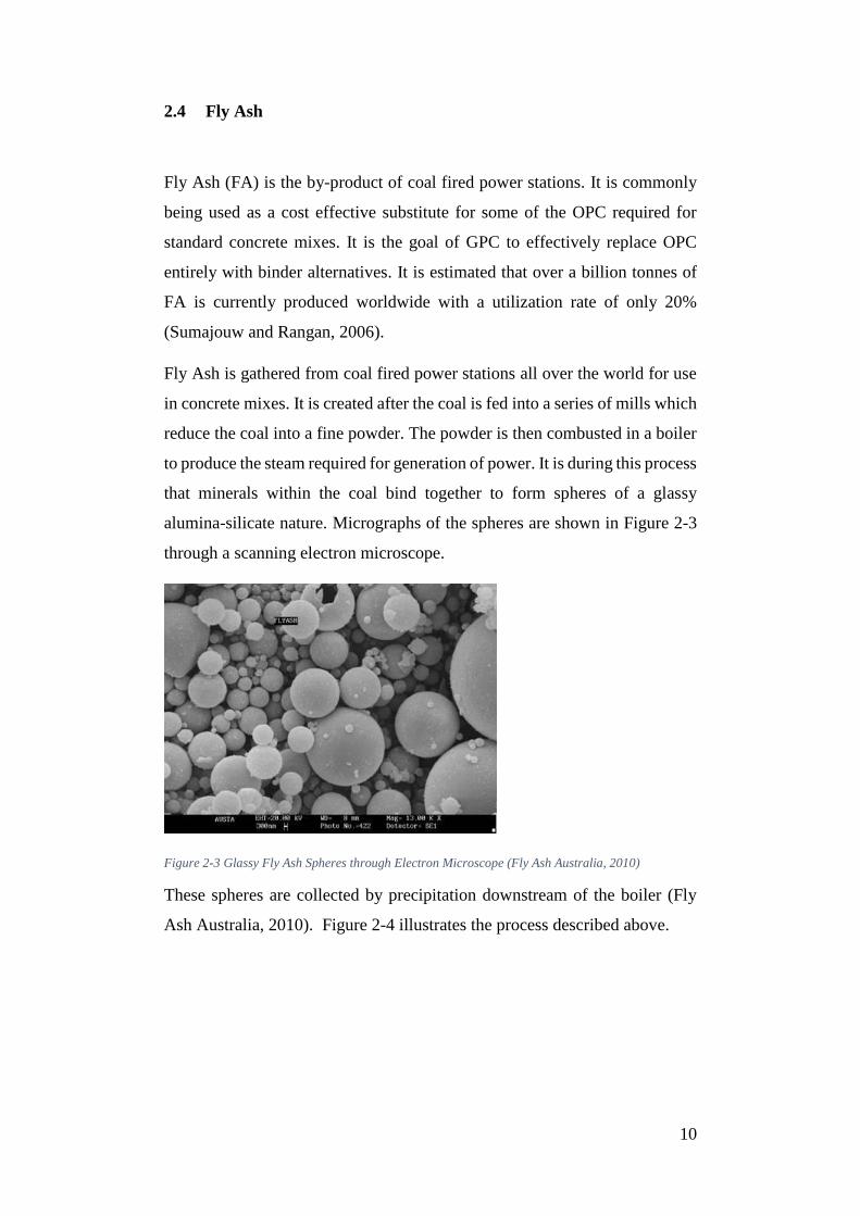
Fly Ash is gathered from coal fired power stations all over the world for use

in concrete mixes. It is created after the coal is fed into a series of mills which

reduce the coal into a fine powder. The powder is then combusted in a boiler

to produce the steam required for generation of power. It is during this process

that minerals within the coal bind together to form spheres of a glassy

alumina-silicate nature. Micrographs of the spheres are shown in Figure 2-3

through a scanning electron microscope.

Figure 2-3 Glassy Fly Ash Spheres through Electron Microscope (Fly Ash Australia, 2010)

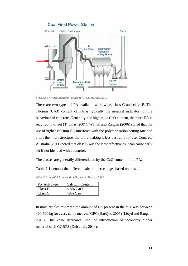
These spheres are collected by precipitation downstream of the boiler (Fly

Ash Australia, 2010). Figure 2-4 illustrates the process described above.

11

Figure 2-4 Fly Ash Retrieval Process (Fly Ash Australia, 2010)

There are two types of FA available worldwide, class C and class F. The

calcium (CaO) content of FA is typically the greatest indicator for the

behaviour of concrete. Generally, the higher the CaO content, the more FA is

required to offset (Thomas, 2007). Wallah and Rangan (2006) stated that the

use of higher calcium FA interferes with the polymerisation setting rate and

alters the microstructure, therefore making it less desirable for use. Concrete

Australia (2011) noted that class C was the least effective as it can cause early

set if not blended with a retarder.

The classes are generally differentiated by the CaO content of the FA.

Table 2-1 denotes the different calcium percentages based on mass.

Table 2-1 Fly Ash Classes and CaO content (Thomas 2007)

Fly Ash Type Calcium Content

Class F < 8% CaO

Class C >8% Cao

In most articles reviewed the amount of FA present in the mix was between

400-500 kg for every cubic metre of GPC (Hardjito 2005) (Lloyd and Rangan,

2010). This value decreases with the introduction of secondary binder

material such GGBFS (Deb et al., 2014).

12

2.5 Ground-granulated Blast-furnace Slag

Ground-granulated Blast-furnace Slag (GGBFS) is another by-product of

industry commonly used in the OPC concrete mix design. It is generally used

to lower heat hydration, resist abrasion wearing from ground water or combat

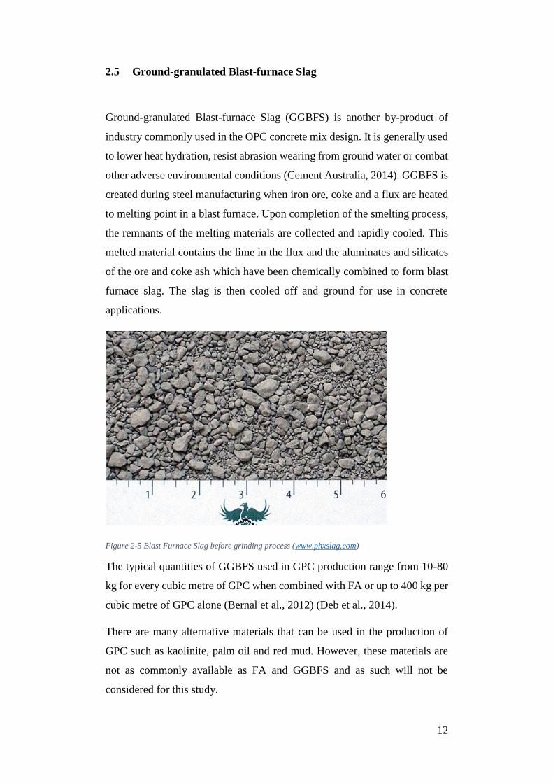
other adverse environmental conditions (Cement Australia, 2014). GGBFS is

created during steel manufacturing when iron ore, coke and a flux are heated

to melting point in a blast furnace. Upon completion of the smelting process,

the remnants of the melting materials are collected and rapidly cooled. This

melted material contains the lime in the flux and the aluminates and silicates

of the ore and coke ash which have been chemically combined to form blast

furnace slag. The slag is then cooled off and ground for use in concrete

applications.

Figure 2-5 Blast Furnace Slag before grinding process (www.phxslag.com)

The typical quantities of GGBFS used in GPC production range from 10-80

kg for every cubic metre of GPC when combined with FA or up to 400 kg per

cubic metre of GPC alone (Bernal et al., 2012) (Deb et al., 2014).

There are many alternative materials that can be used in the production of

GPC such as kaolinite, palm oil and red mud. However, these materials are

not as commonly available as FA and GGBFS and as such will not be

considered for this study.

13

2.6 Alkaline Activators

The activators required to complete the polymerisation process are typically

sodium silicate (SiO2/Na2O) and sodium hydroxide (NaOH) solutions. The

higher the NaOH content the higher the resultant compressive strength

(Hardjito, 2005). Potassium based hydroxide solutions are able to be used

instead of the NaOH solutions but are generally ignored due to the higher

associated costs, (Hardjito and Rangan, 2005).

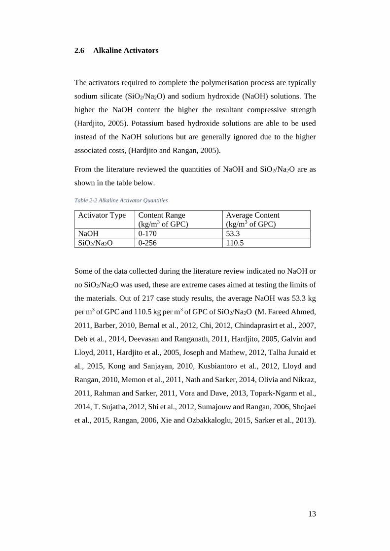
From the literature reviewed the quantities of NaOH and SiO2/Na2O are as

shown in the table below.

Table 2-2 Alkaline Activator Quantities

Activator Type Content Range

(kg/m3 of GPC)

Average Content

(kg/m3 of GPC)

NaOH 0-170 53.3

SiO2/Na2O 0-256 110.5

Some of the data collected during the literature review indicated no NaOH or

no SiO2/Na2O was used, these are extreme cases aimed at testing the limits of

the materials. Out of 217 case study results, the average NaOH was 53.3 kg

per m3 of GPC and 110.5 kg per m3 of GPC of SiO2/Na2O (M. Fareed Ahmed,

2011, Barber, 2010, Bernal et al., 2012, Chi, 2012, Chindaprasirt et al., 2007,

Deb et al., 2014, Deevasan and Ranganath, 2011, Hardjito, 2005, Galvin and

Lloyd, 2011, Hardjito et al., 2005, Joseph and Mathew, 2012, Talha Junaid et

al., 2015, Kong and Sanjayan, 2010, Kusbiantoro et al., 2012, Lloyd and

Rangan, 2010, Memon et al., 2011, Nath and Sarker, 2014, Olivia and Nikraz,

2011, Rahman and Sarker, 2011, Vora and Dave, 2013, Topark-Ngarm et al.,

2014, T. Sujatha, 2012, Shi et al., 2012, Sumajouw and Rangan, 2006, Shojaei

et al., 2015, Rangan, 2006, Xie and Ozbakkaloglu, 2015, Sarker et al., 2013).

14

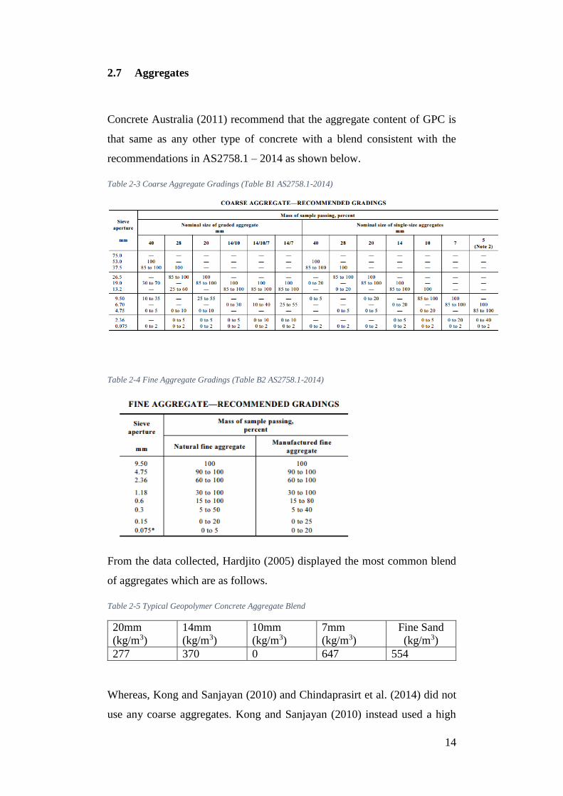
2.7 Aggregates

Concrete Australia (2011) recommend that the aggregate content of GPC is

that same as any other type of concrete with a blend consistent with the

recommendations in AS2758.1 – 2014 as shown below.

Table 2-3 Coarse Aggregate Gradings (Table B1 AS2758.1-2014)

Table 2-4 Fine Aggregate Gradings (Table B2 AS2758.1-2014)

From the data collected, Hardjito (2005) displayed the most common blend

of aggregates which are as follows.

Table 2-5 Typical Geopolymer Concrete Aggregate Blend

20mm

(kg/m3)

14mm

(kg/m3)

10mm

(kg/m3)

7mm

(kg/m3)

Fine Sand

(kg/m3)

277 370 0 647 554

Whereas, Kong and Sanjayan (2010) and Chindaprasirt et al. (2014) did not

use any coarse aggregates. Kong and Sanjayan (2010) instead used a high

15

volume of slag to compensate, and Chindaprasirt et al. (2014) used higher

volumes FA and fine sand. Both resulted in comparable compression

strengths.

Others used no 20mm or 14mm aggregates and instead made up the quanities

using more 10mm, 7mm and Fine Sand. All total quantities of aggregates

were approximately 1850kg per m3 of GPC which is approximately 80% of

the total weight (Deevasan and Ranganath 2011, Hardjito, D., et al. 2005,

Olivia and Nikraz 2011, Bernal, Mejía de Gutiérrez et al. 2012, Chi 2012,

Shojaei, Behfarnia et al. 2015, Deb, Nath et al. 2014, Nath and Sarker 2014,

Topark-Ngarm, Chindaprasirt et al. 2014).

2.8 Super Plasticizer

Wallah and Rangan (2006) describes that super plasticizers (SP) were

required to improve the workability of the fresh GPC concrete. As such, “a

high-range water-reducing Naphthalene based super plasticizer was added to

the mixture” (Wallah and Rangan 2006).

Wallah and Rangan (2006) added 6kg per m3 of GPC to all of their mixes.

This quantity was also similar to other research, with SP ranging from 6-12

kg per m3 of GPC (Hardjito 2005, Hardjito, Wallah et al. 2005, Rangan 2006,

Barber 2010, Kong and Sanjayan 2010, Lloyd and Rangan 2010, Galvin and

Lloyd 2011, M. Fareed Ahmed 2011, Memon, Nuruddin et al. 2011, Olivia

and Nikraz 2011, Rahman and Sarker 2011, Joseph and Mathew 2012,

Kusbiantoro, Nuruddin et al. 2012, T. Sujatha 2012, Sarker, Haque et al.

2013, Vora and Dave 2013, Deb, Nath et al. 2014, Nath and Sarker 2014,

Topark-Ngarm, Chindaprasirt et al. 2014, Shojaei, Behfarnia et al. 2015,

Talha Junaid, Kayali et al. 2015, Xie and Ozbakkaloglu 2015).

Chindaprasirt, Chareerat et al. (2007) had quantities of SP ranging from 0-60

kg per m3 of GPC, the higher quantities were used to compensate for the high

calcium content of the class C FA used.

16

2.9 Compressive Strength Prediction

Recent studies have relied on the use of Artificial Neural Networks (ANN) to

help predict compressive strength of GPC with different binding materials

(Nazari and Torgal, 2012, Bondar, 2011). ANNs are described as a series of

parallel architectures that work cooperatively to solve complex problems by

connecting simple computing elements (Nazari and Torgal, 2012). The

networks utilise learning capabilities obtained from example inputs, which

make them perfect for use for the prediction of GPC compressive strength as

available data is fairly limited.

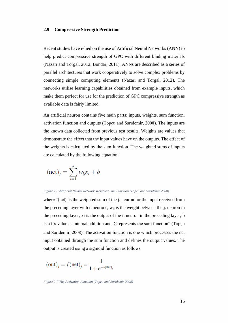
An artificial neuron contains five main parts: inputs, weights, sum function,

activation function and outputs (Topçu and Sarıdemir, 2008). The inputs are

the known data collected from previous test results. Weights are values that

demonstrate the effect that the input values have on the outputs. The effect of

the weights is calculated by the sum function. The weighted sums of inputs

are calculated by the following equation:

Figure 2-6 Artificial Neural Network Weighted Sum Function (Topcu and Saridemir 2008)

where “(net)j is the weighted sum of the j. neuron for the input received from

the preceding layer with n neurons, wij is the weight between the j. neuron in

the preceding layer, xi is the output of the i. neuron in the preceding layer, b

is a fix value as internal addition and Σrepresents the sum function” (Topçu

and Sarıdemir, 2008). The activation function is one which processes the net

input obtained through the sum function and defines the output values. The

output is created using a sigmoid function as follows

Figure 2-7 The Activation Function (Topcu and Saridemir 2008)

17

Where α is a constant used to control the slope of the semi-linear region

(Topcu and Saridemir 2008).

In recent years, ANNs have been used in the civil engineering industry to

overcome many problems such as determining structural damage, the

modelling of material behaviour, and ground water monitoring (Topçu et al.,

2008).

Topcu, Karakurt et al. (2008) used ANNs along with fuzzy logic to predict

the strength development of GPC with different binding materials. They

found that compressive strengths can be predicted through the use of ANNs

in a short period of time with minimal error in comparison to test results.

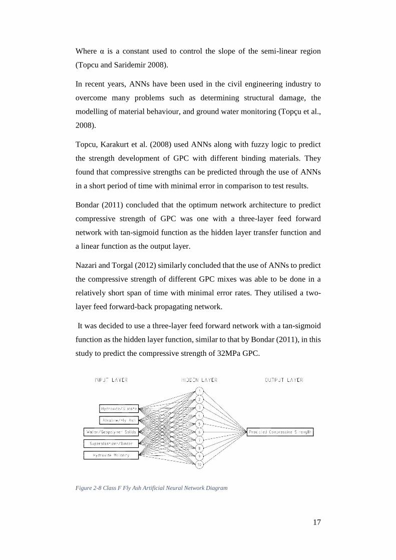
Bondar (2011) concluded that the optimum network architecture to predict

compressive strength of GPC was one with a three-layer feed forward

network with tan-sigmoid function as the hidden layer transfer function and

a linear function as the output layer.

Nazari and Torgal (2012) similarly concluded that the use of ANNs to predict

the compressive strength of different GPC mixes was able to be done in a

relatively short span of time with minimal error rates. They utilised a two-

layer feed forward-back propagating network.

It was decided to use a three-layer feed forward network with a tan-sigmoid

function as the hidden layer function, similar to that by Bondar (2011), in this

study to predict the compressive strength of 32MPa GPC.

Figure 2-8 Class F Fly Ash Artificial Neural Network Diagram

18

CHAPTER 3 MIX PROPORTIONS AND DATABASE

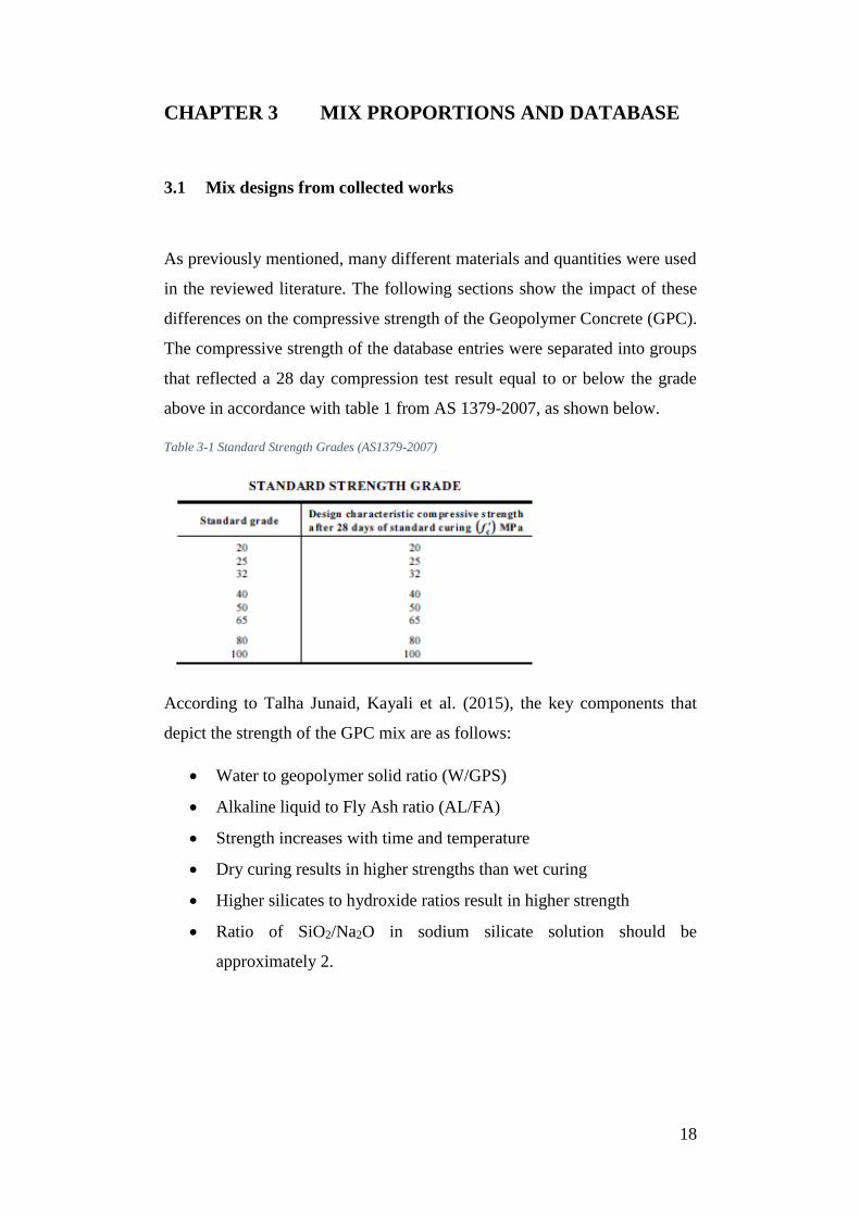
3.1 Mix designs from collected works

As previously mentioned, many different materials and quantities were used

in the reviewed literature. The following sections show the impact of these

differences on the compressive strength of the Geopolymer Concrete (GPC).

The compressive strength of the database entries were separated into groups

that reflected a 28 day compression test result equal to or below the grade

above in accordance with table 1 from AS 1379-2007, as shown below.

Table 3-1 Standard Strength Grades (AS1379-2007)

According to Talha Junaid, Kayali et al. (2015), the key components that

depict the strength of the GPC mix are as follows:

Water to geopolymer solid ratio (W/GPS)

Alkaline liquid to Fly Ash ratio (AL/FA)

Strength increases with time and temperature

Dry curing results in higher strengths than wet curing

Higher silicates to hydroxide ratios result in higher strength

Ratio of SiO2/Na2O in sodium silicate solution should be

approximately 2.

19

3.1.1 Water to Geopolymer Solid Ratio

The water to geopolymer solid ratio (W/GPS) is the total mass of water in the

system, including that used in the alkaline solution and extra water, divided

by the total mass of the Fly Ash, Ground-granulated Blast-furnace Slag

(GGBFS), sodium hydroxide pellets/flakes and sodium silicate solids

(Ferdous et al., 2015). This ratio works in the same fashion as the

water/cement ratio in OPC.

Figure 3-1 Compressive Strength to Water/Geopolymer Solids Ratio (Ferdous, Manalo et al. 2015)

As shown in Figure 3-1Error! Reference source not found., the W/GPS

atio has a direct effect on the strength of the concrete. The lower W/GPS

results in higher strength concrete but is difficult to work with due to the

dryness of the mix (Ferdous, Manalo et al. 2015). Based on Error! Reference

ource not found., the W/GPS ratio for 32MPa concrete is approximately

0.37. Lloyd, N. A. and B. V. Rangan (2010) indicated that the W/GPS ratio

need not be this high to achieve 32MPa concrete. As shown in Table 3-2, the

W/GPS ratio should be approximately 0.23. This would result in a highly

workable mix based on 400kg of FA per cubic metre of GPC. The values

given are dependent on the notion that all aggregates are in the saturated

surface dry condition.

20

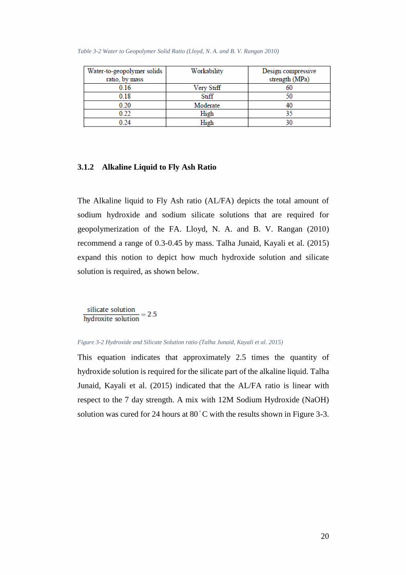
Table 3-2 Water to Geopolymer Solid Ratio (Lloyd, N. A. and B. V. Rangan 2010)

3.1.2 Alkaline Liquid to Fly Ash Ratio

The Alkaline liquid to Fly Ash ratio (AL/FA) depicts the total amount of

sodium hydroxide and sodium silicate solutions that are required for

geopolymerization of the FA. Lloyd, N. A. and B. V. Rangan (2010)

recommend a range of 0.3-0.45 by mass. Talha Junaid, Kayali et al. (2015)

expand this notion to depict how much hydroxide solution and silicate

solution is required, as shown below.

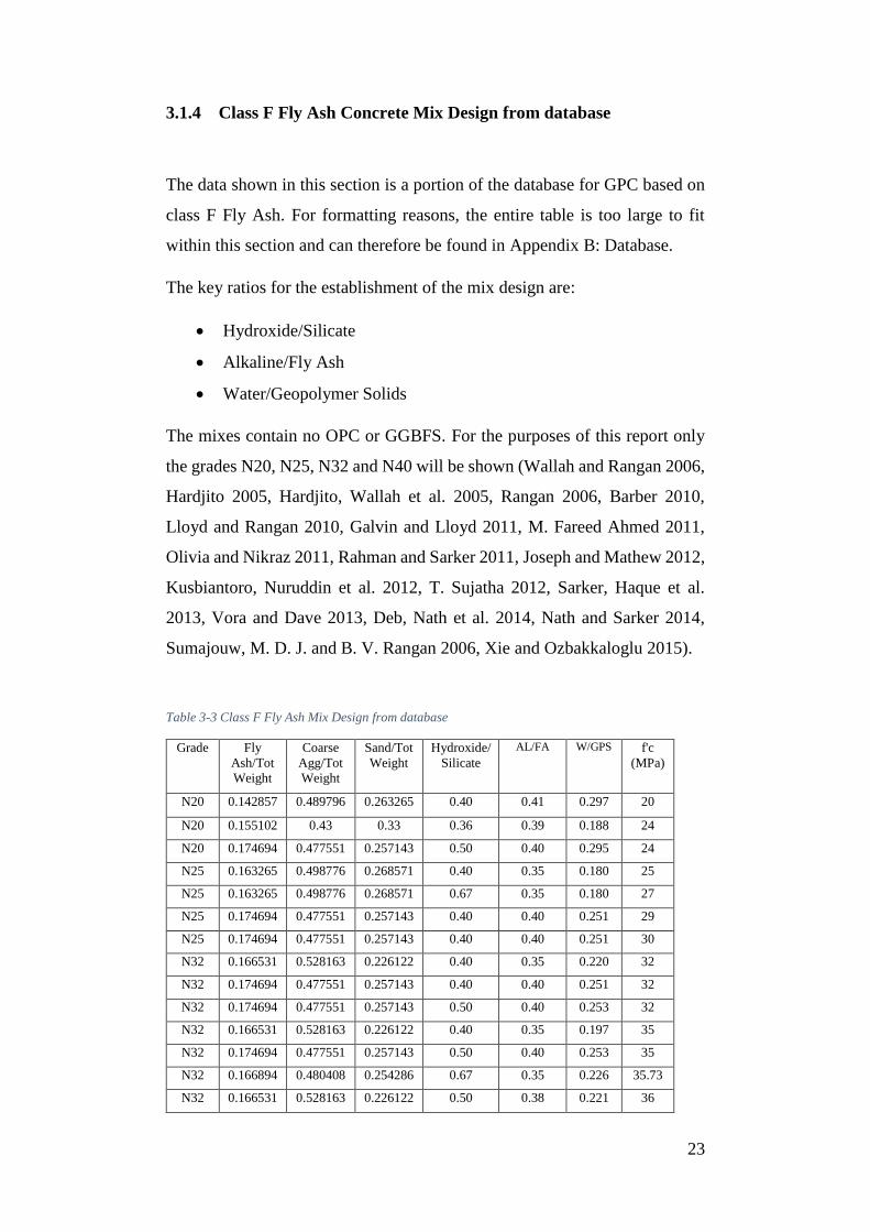
Figure 3-2 Hydroxide and Silicate Solution ratio (Talha Junaid, Kayali et al. 2015)

This equation indicates that approximately 2.5 times the quantity of

hydroxide solution is required for the silicate part of the alkaline liquid. Talha

Junaid, Kayali et al. (2015) indicated that the AL/FA ratio is linear with

respect to the 7 day strength. A mix with 12M Sodium Hydroxide (NaOH)

solution was cured for 24 hours at 80°C with the results shown in Figure 3-3.

21

Figure 3-3 Alkaline/Fly Ash Vs 7 Day Strength for 12M Sodium Hydroxide Solution after 24 hours

curing (Talha Junaid, Kayali et al. 2015)

Based on 32MPa concrete for medium workability and a W/GPS ratio of 0.27,

the graph above would indicate an AL/FA ratio of approximately 0.4 which

corresponds to the research by Lloyd, N. A. and B. V. Rangan (2010). This

value is also used by Shojaei, M., et al. (2015) for the AL/GGBFS ratio. For

this report the value of 0.4 will be the desired ratio for all mixes whether they

be based on FA only, Ground-granulated Blast-furnace Slag (GGBFS) only,

or a combination of FA and GGBFS.

22

3.1.3 Mix Design Database

After the literature review was complete, a database was established from a

number of published articles based on the following criterion:

1. Only FA and GGBFS mixes would be included

2. A mix design could only be included once, duplicates from same

authors were excluded

3. Extreme or out-of-the-ordinary mixes were excluded

As previously established, only FA and GGBFS mixes would be used as these

materials are readily available in the Australian construction industry. Mixes

containing other materials were not included due to ease of access and

therefore cost.

Many authors re-used mix designs for different research purposes such as acid

resistance, fire resistance, etc. Each mix still gave the same compressive

strength. As such a mix design could only be included once.

Some authors used extremely high percentages of materials to test the impact

on the overall mix. These mixes were excluded as they did not represent

typical construction purposes.

23

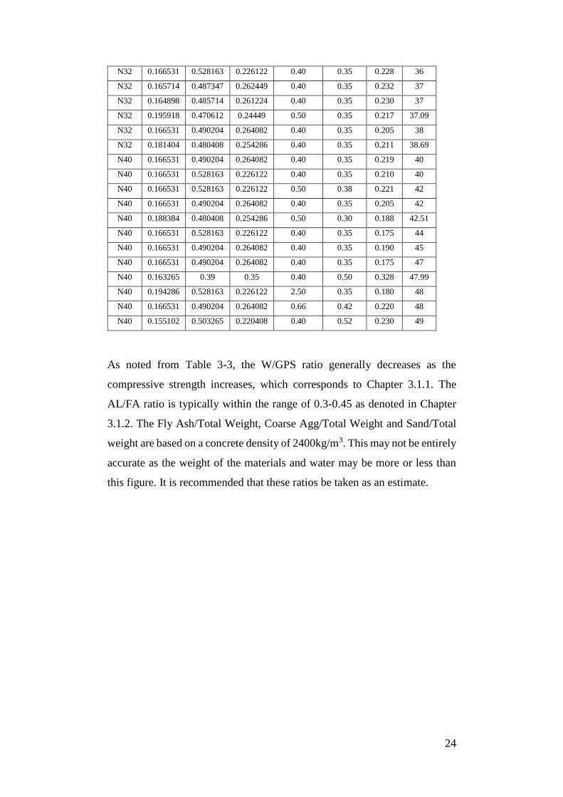
3.1.4 Class F Fly Ash Concrete Mix Design from database

The data shown in this section is a portion of the database for GPC based on

class F Fly Ash. For formatting reasons, the entire table is too large to fit

within this section and can therefore be found in Appendix B: Database.

The key ratios for the establishment of the mix design are:

Hydroxide/Silicate

Alkaline/Fly Ash

Water/Geopolymer Solids

The mixes contain no OPC or GGBFS. For the purposes of this report only

the grades N20, N25, N32 and N40 will be shown (Wallah and Rangan 2006,

Hardjito 2005, Hardjito, Wallah et al. 2005, Rangan 2006, Barber 2010,

Lloyd and Rangan 2010, Galvin and Lloyd 2011, M. Fareed Ahmed 2011,

Olivia and Nikraz 2011, Rahman and Sarker 2011, Joseph and Mathew 2012,

Kusbiantoro, Nuruddin et al. 2012, T. Sujatha 2012, Sarker, Haque et al.

2013, Vora and Dave 2013, Deb, Nath et al. 2014, Nath and Sarker 2014,

Sumajouw, M. D. J. and B. V. Rangan 2006, Xie and Ozbakkaloglu 2015).

Table 3-3 Class F Fly Ash Mix Design from database

Grade Fly

Ash/Tot

Weight

Coarse

Agg/Tot

Weight

Sand/Tot

Weight

Hydroxide/

Silicate

AL/FA W/GPS f'c

(MPa)

N20 0.142857 0.489796 0.263265 0.40 0.41 0.297 20

N20 0.155102 0.43 0.33 0.36 0.39 0.188 24

N20 0.174694 0.477551 0.257143 0.50 0.40 0.295 24

N25 0.163265 0.498776 0.268571 0.40 0.35 0.180 25

N25 0.163265 0.498776 0.268571 0.67 0.35 0.180 27

N25 0.174694 0.477551 0.257143 0.40 0.40 0.251 29

N25 0.174694 0.477551 0.257143 0.40 0.40 0.251 30

N32 0.166531 0.528163 0.226122 0.40 0.35 0.220 32

N32 0.174694 0.477551 0.257143 0.40 0.40 0.251 32

N32 0.174694 0.477551 0.257143 0.50 0.40 0.253 32

N32 0.166531 0.528163 0.226122 0.40 0.35 0.197 35

N32 0.174694 0.477551 0.257143 0.50 0.40 0.253 35

N32 0.166894 0.480408 0.254286 0.67 0.35 0.226 35.73

N32 0.166531 0.528163 0.226122 0.50 0.38 0.221 36

24

N32 0.166531 0.528163 0.226122 0.40 0.35 0.228 36

N32 0.165714 0.487347 0.262449 0.40 0.35 0.232 37

N32 0.164898 0.485714 0.261224 0.40 0.35 0.230 37

N32 0.195918 0.470612 0.24449 0.50 0.35 0.217 37.09

N32 0.166531 0.490204 0.264082 0.40 0.35 0.205 38

N32 0.181404 0.480408 0.254286 0.40 0.35 0.211 38.69

N40 0.166531 0.490204 0.264082 0.40 0.35 0.219 40

N40 0.166531 0.528163 0.226122 0.40 0.35 0.210 40

N40 0.166531 0.528163 0.226122 0.50 0.38 0.221 42

N40 0.166531 0.490204 0.264082 0.40 0.35 0.205 42

N40 0.188384 0.480408 0.254286 0.50 0.30 0.188 42.51

N40 0.166531 0.528163 0.226122 0.40 0.35 0.175 44

N40 0.166531 0.490204 0.264082 0.40 0.35 0.190 45

N40 0.166531 0.490204 0.264082 0.40 0.35 0.175 47

N40 0.163265 0.39 0.35 0.40 0.50 0.328 47.99

N40 0.194286 0.528163 0.226122 2.50 0.35 0.180 48

N40 0.166531 0.490204 0.264082 0.66 0.42 0.220 48

N40 0.155102 0.503265 0.220408 0.40 0.52 0.230 49

As noted from Table 3-3, the W/GPS ratio generally decreases as the

compressive strength increases, which corresponds to Chapter 3.1.1. The

AL/FA ratio is typically within the range of 0.3-0.45 as denoted in Chapter

3.1.2. The Fly Ash/Total Weight, Coarse Agg/Total Weight and Sand/Total

weight are based on a concrete density of 2400kg/m3. This may not be entirely

accurate as the weight of the materials and water may be more or less than

this figure. It is recommended that these ratios be taken as an estimate.

25

3.1.5 Class C Fly Ash Concrete Mix Design from database


class C Fly Ash, see Appendix B: Database for the full database. The mixes

contain no OPC or GGBFS. For the purposes of this report only the grades

N25, N32 and N40 will be shown (Chindaprasirt, P., et al. 2007, Topark-

Ngarm, P., et al. 2014).

Table 3-4 Class C Fly Ash Mix Design from database

Grade Fly

Ash/Tot

Weight

Coarse

Agg/Tot

Weight

Sand/Tot

Weight

Hydroxide/

Silicate

AL/FA W/GPS f'c (MPa)

N25 0.21 0.00 0.56 0.49 0.51 0.295 26

N25 0.21 0.00 0.56 1.00 0.51 0.293 30

N32 0.21 0.00 0.56 0.50 0.51 0.295 32

N32 0.17 0.45 0.24 0.50 0.50 0.222 33.8

N32 0.21 0.00 0.56 0.49 0.51 0.239 36

N32 0.17 0.45 0.24 1.00 0.50 0.229 37.64

N32 0.21 0.00 0.56 0.49 0.51 0.267 38

N32 0.17 0.45 0.24 0.50 0.50 0.222 39.02

N40 0.17 0.45 0.24 1.00 0.50 0.229 39.67

N40 0.21 0.00 0.56 2.00 0.51 0.272 40

N40 0.21 0.00 0.56 2.00 0.51 0.300 42

N40 0.21 0.00 0.56 0.50 0.51 0.267 43

N40 0.21 0.00 0.56 1.00 0.51 0.265 45

N40 0.17 0.45 0.24 1.00 0.50 0.229 45.34

N40 0.17 0.45 0.24 0.50 0.50 0.222 46.69

N40 0.21 0.00 0.56 1.00 0.51 0.237 48

N40 0.21 0.00 0.56 2.00 0.51 0.254 48

As noted in Table 3-4, there are many differences in comparison to the Class

F mix design database. These differences are as follows

Hydroxide/Silicate ratios are much higher for Class C FA

AL/FA ratios are much higher for Class C FA

W/GPS is also higher for Class C FA

This coincides with that denoted in Chapter 2.4 and would explain why the

cost of working with Class C FA would be greater than that found with Class

F FA.

26

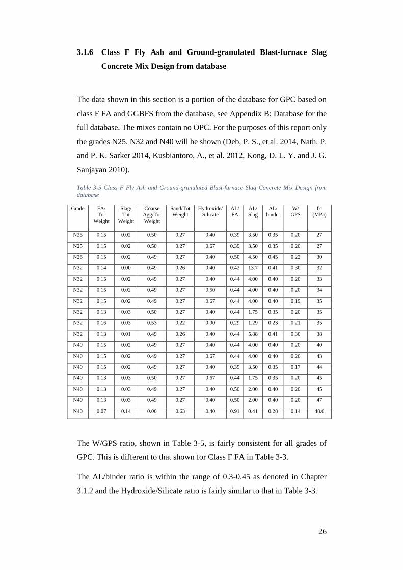
3.1.6 Class F Fly Ash and Ground-granulated Blast-furnace Slag

Concrete Mix Design from database


class F FA and GGBFS from the database, see Appendix B: Database for the

full database. The mixes contain no OPC. For the purposes of this report only

the grades N25, N32 and N40 will be shown (Deb, P. S., et al. 2014, Nath, P.

and P. K. Sarker 2014, Kusbiantoro, A., et al. 2012, Kong, D. L. Y. and J. G.

Sanjayan 2010).

Table 3-5 Class F Fly Ash and Ground-granulated Blast-furnace Slag Concrete Mix Design from

database

Grade FA/ Tot

Weight

Slag/ Tot

Weight

Coarse Agg/Tot

Weight

Sand/Tot Weight

Hydroxide/ Silicate

AL/ FA

AL/ Slag

AL/ binder

W/ GPS

f'c (MPa)

N25 0.15 0.02 0.50 0.27 0.40 0.39 3.50 0.35 0.20 27

N25 0.15 0.02 0.50 0.27 0.67 0.39 3.50 0.35 0.20 27

N25 0.15 0.02 0.49 0.27 0.40 0.50 4.50 0.45 0.22 30

N32 0.14 0.00 0.49 0.26 0.40 0.42 13.7 0.41 0.30 32

N32 0.15 0.02 0.49 0.27 0.40 0.44 4.00 0.40 0.20 33

N32 0.15 0.02 0.49 0.27 0.50 0.44 4.00 0.40 0.20 34

N32 0.15 0.02 0.49 0.27 0.67 0.44 4.00 0.40 0.19 35

N32 0.13 0.03 0.50 0.27 0.40 0.44 1.75 0.35 0.20 35

N32 0.16 0.03 0.53 0.22 0.00 0.29 1.29 0.23 0.21 35

N32 0.13 0.01 0.49 0.26 0.40 0.44 5.88 0.41 0.30 38

N40 0.15 0.02 0.49 0.27 0.40 0.44 4.00 0.40 0.20 40

N40 0.15 0.02 0.49 0.27 0.67 0.44 4.00 0.40 0.20 43

N40 0.15 0.02 0.49 0.27 0.40 0.39 3.50 0.35 0.17 44

N40 0.13 0.03 0.50 0.27 0.67 0.44 1.75 0.35 0.20 45

N40 0.13 0.03 0.49 0.27 0.40 0.50 2.00 0.40 0.20 45

N40 0.13 0.03 0.49 0.27 0.40 0.50 2.00 0.40 0.20 47

N40 0.07 0.14 0.00 0.63 0.40 0.91 0.41 0.28 0.14 48.6

The W/GPS ratio, shown in Table 3-5, is fairly consistent for all grades of

GPC. This is different to that shown for Class F FA in Table 3-3.

The AL/binder ratio is within the range of 0.3-0.45 as denoted in Chapter

3.1.2 and the Hydroxide/Silicate ratio is fairly similar to that in Table 3-3.

27

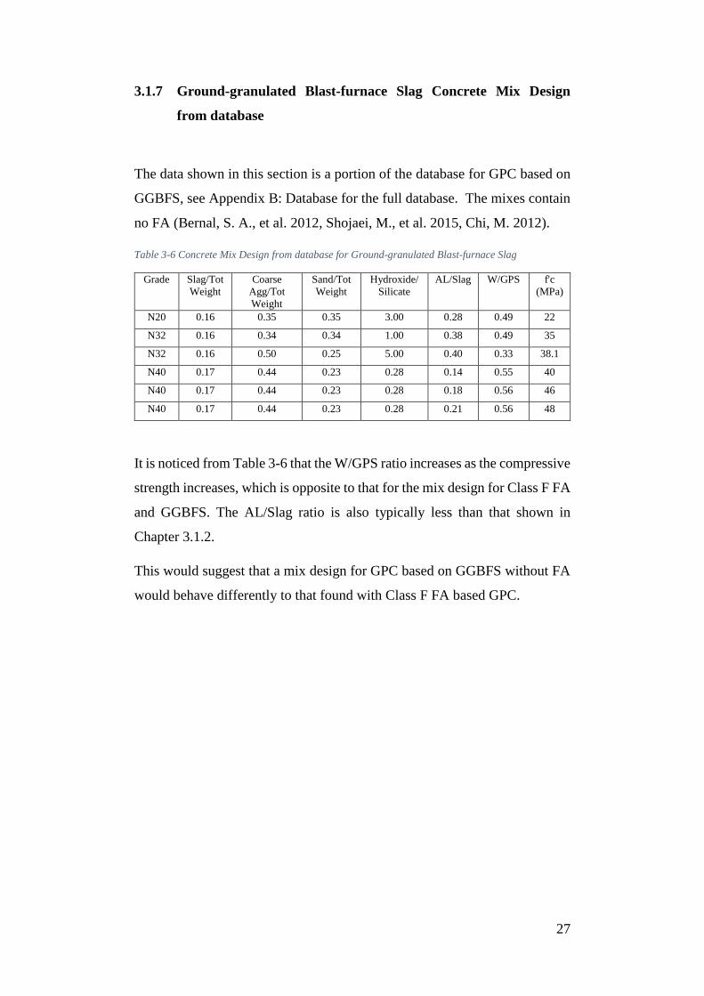
3.1.7 Ground-granulated Blast-furnace Slag Concrete Mix Design

from database


GGBFS, see Appendix B: Database for the full database. The mixes contain

no FA (Bernal, S. A., et al. 2012, Shojaei, M., et al. 2015, Chi, M. 2012).

Table 3-6 Concrete Mix Design from database for Ground-granulated Blast-furnace Slag

Grade Slag/Tot

Weight

Coarse

Agg/Tot

Weight

Sand/Tot

Weight

Hydroxide/

Silicate

AL/Slag W/GPS f'c

(MPa)

N20 0.16 0.35 0.35 3.00 0.28 0.49 22

N32 0.16 0.34 0.34 1.00 0.38 0.49 35

N32 0.16 0.50 0.25 5.00 0.40 0.33 38.1

N40 0.17 0.44 0.23 0.28 0.14 0.55 40

N40 0.17 0.44 0.23 0.28 0.18 0.56 46

N40 0.17 0.44 0.23 0.28 0.21 0.56 48

It is noticed from Table 3-6 that the W/GPS ratio increases as the compressive

strength increases, which is opposite to that for the mix design for Class F FA

and GGBFS. The AL/Slag ratio is also typically less than that shown in

Chapter 3.1.2.

This would suggest that a mix design for GPC based on GGBFS without FA

would behave differently to that found with Class F FA based GPC.

28

CHAPTER 4 ARTIFICIAL NEURAL NETWORK

DEVELOPMENT

As previously mentioned, the study will use Artificial Neural Networks

(ANN) to ascertain an optimum mix design for 32MPa Geopolymer Concrete

(GPC). It was decided to create ANNs for all available mix design options for

Fly Ash (FA) and Ground-granulated Blast-furnace Slag (GGBFS) for

comparison of the mix designs and give the option to use either mix of

materials.

To create the networks, the following inputs were taken from the database

and fed into the neural network toolbox in Matlab.

1. Hydroxide /Sodium Silicate ratio

2. Alkaline Liquid/Fly Ash Ratio or Alkaline Liquid/Binder Ratio

3. Water/Geopolymer Solids

4. The Molarity of the Hydroxide solution

5. Superplasticizers/binder ratio

As mentioned in Chapter 2.9, it was decided to use a three-layer feed forward

network with a tan-sigmoid function as the hidden layer function in this study

to predict the compressive strength of 32MPa GPC.

Once the input and target data were arranged and entered into Matlab the

ANNs were then able to be created. This was done by using the Matlab

NNTOOL function. The NN toolbox allows you to enter data, train it and also

simulate it, as well as many other functions which are not the focus of this

project.

Bondar (2011) describes the feed forward and back propagation method as,

for every interval, an output compressive strength is calculated from the

current weights and biases based on the input data. Then for the second step,

the weights and biases are modified by the back propagation algorithm. The

performance function, mean square error in this case, are also minimised by

this change of weights and biases in each step.

29

The training algorithm used in this project is the traingda algorithm, as offered

in the NN toolbox. Bondar (2011) showed that the traingda algorithm stops

training the data if any of the following conditions are met:

The maximum repetitions or epochs are met

The maximum timeframe has expired

The performance is minimised to suit the target data

The gradient of performance falls below min_grad

The training performances and outputs for the ANNs are shown in the

following sections.

30

4.1 Class F Fly Ash and Ground-granulated Blast-furnace Slag

Artificial Neural Network

The ANN was created based on Class F Fly Ash (FA) and Ground-granulated

Blast-furnace Slag (GGBFS) as the binding material input presented in Table

3-5 and Appendix B: Database. As shown in Table 4-1, this network had 7

inputs and 1 output, being the compressive strengths.

Table 4-1 Class F Fly Ash and Ground-granulated Blast-furnace Slag Artificial Neural Network Inputs

and Predicted Outputs

NaOH/

Sodium

Silicate

AL/FA AL/Slag AL/Binder W/GPS Super/

Binder

NaOH

Molarity

Actual

Comp.

Strength

(MPa)

Predicted

Comp.

Strength

(MPa)

0.40 0.44 5.88 0.41 0.30 0 8 15 31.45674

0.40 0.42 13.71 0.41 0.30 0 8 18 26.20466

0.40 0.39 3.50 0.35 0.20 0.015 14 27 30.10456

0.67 0.39 3.50 0.35 0.20 0.015 14 27 24.92903

0.40 0.50 4.50 0.45 0.22 0 12 30 32.28533

0.40 0.42 13.71 0.41 0.30 0 8 32 26.20466

0.40 0.44 4.00 0.40 0.20 0 12 33 32.98397

0.50 0.44 4.00 0.40 0.20 0 12 34 31.15133

0.67 0.44 4.00 0.40 0.19 0 12 35 30.55009

0.40 0.44 1.75 0.35 0.20 0.015 14 35 28.77511

0.00 0.29 1.29 0.23 0.21 0 12 35 40.98999

0.40 0.44 5.88 0.41 0.30 0 8 38 31.45674

0.40 0.44 4.00 0.40 0.20 0 14 40 43.13738

0.67 0.44 4.00 0.40 0.20 0 14 43 39.28931

0.40 0.39 3.50 0.35 0.17 0 12 44 35.40669

0.67 0.44 1.75 0.35 0.20 0.015 14 45 25.59835

0.40 0.50 2.00 0.40 0.20 0 12 45 31.07638

0.40 0.50 2.00 0.40 0.20 0 14 47 41.65267

0.40 0.91 0.41 0.28 0.14 0 8 48.6 44.11854

0.40 0.92 0.42 0.29 0.14 0 8 52.8 43.82771

0.67 0.50 2.00 0.40 0.20 0 14 54 39.70501

0.40 0.92 0.42 0.29 0.14 0 8 54 43.82771

0.40 0.57 1.33 0.40 0.20 0 12 55 30.99393

0.40 1.36 0.62 0.42 0.20 0 8 55.4 49.46125

0.40 0.33 0.12 0.09 0.05 0 12 61.8 55.15615

31

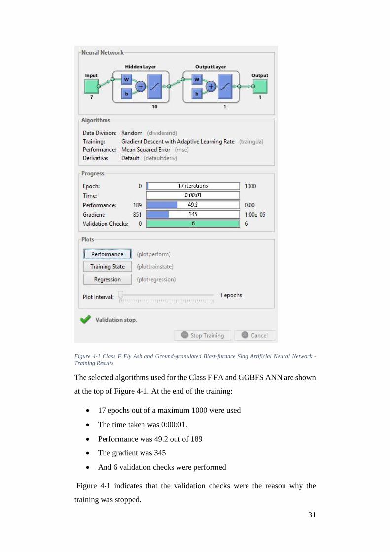
Figure 4-1 Class F Fly Ash and Ground-granulated Blast-furnace Slag Artificial Neural Network -

Training Results

The selected algorithms used for the Class F FA and GGBFS ANN are shown

at the top of Figure 4-1. At the end of the training:

17 epochs out of a maximum 1000 were used

The time taken was 0:00:01.

Performance was 49.2 out of 189

The gradient was 345

And 6 validation checks were performed

Figure 4-1 indicates that the validation checks were the reason why the

training was stopped.

32

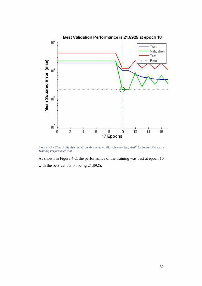
Figure 4-2 - Class F Fly Ash and Ground-granulated Blast-furnace Slag Artificial Neural Network -

Training Performance Plot

As shown in Figure 4-2, the performance of the training was best at epoch 10

with the best validation being 21.8925.

33

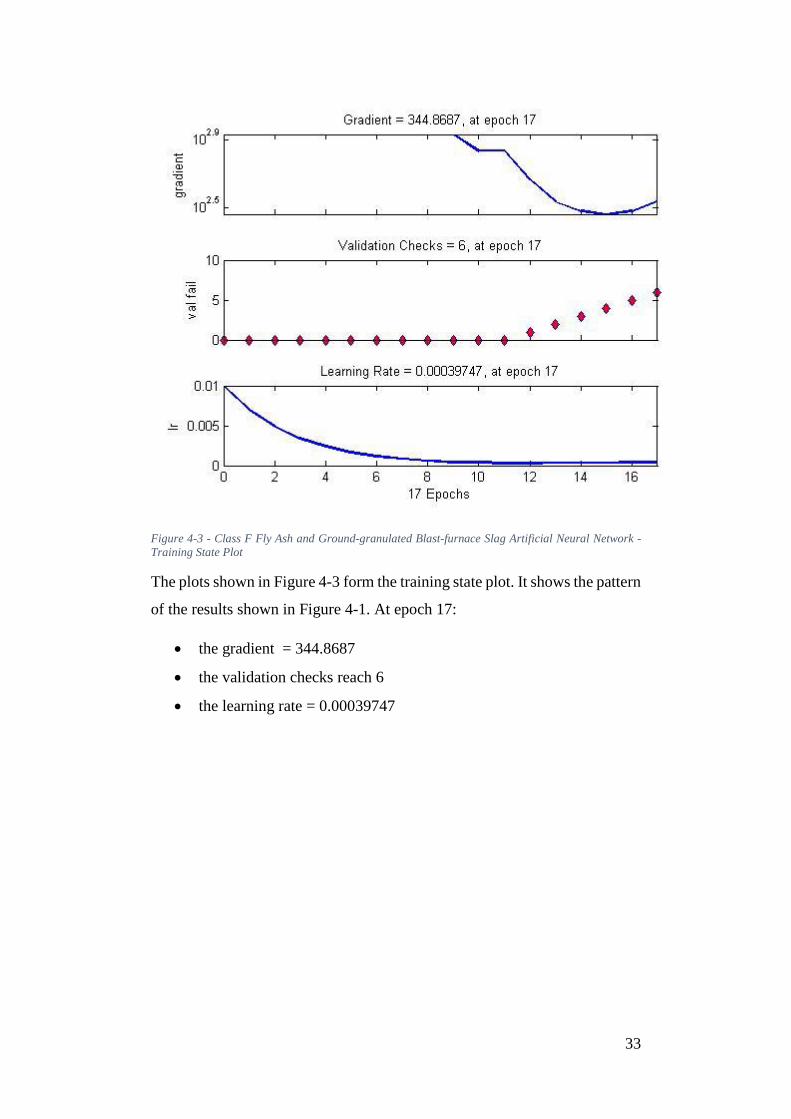
Figure 4-3 - Class F Fly Ash and Ground-granulated Blast-furnace Slag Artificial Neural Network -

Training State Plot

The plots shown in Figure 4-3 form the training state plot. It shows the pattern

of the results shown in Figure 4-1. At epoch 17:

the gradient = 344.8687

the validation checks reach 6

the learning rate = 0.00039747

34

Figure 4-4- Class F Fly Ash and Ground-granulated Blast-furnace Slag Artificial Neural Network -

Training Regression Plots

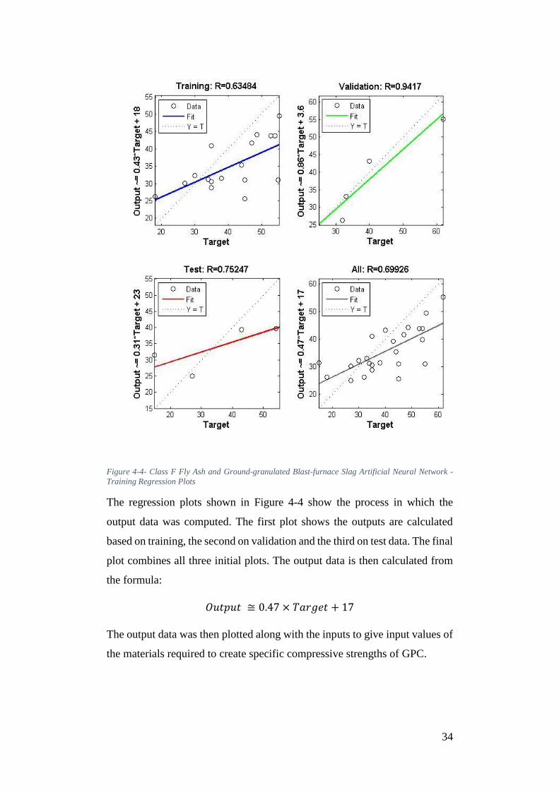
The regression plots shown in Figure 4-4 show the process in which the

output data was computed. The first plot shows the outputs are calculated

based on training, the second on validation and the third on test data. The final

plot combines all three initial plots. The output data is then calculated from

the formula:

𝑂𝑢𝑡𝑝𝑢𝑡 ≅ 0.47 × 𝑇𝑎𝑟𝑔𝑒𝑡 + 17

The output data was then plotted along with the inputs to give input values of

the materials required to create specific compressive strengths of GPC.

35

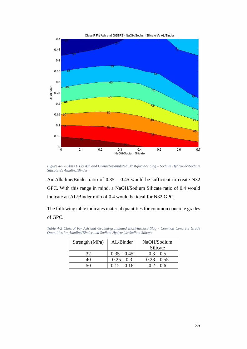
Figure 4-5 - Class F Fly Ash and Ground-granulated Blast-furnace Slag – Sodium Hydroxide/Sodium

Silicate Vs Alkaline/Binder

An Alkaline/Binder ratio of 0.35 – 0.45 would be sufficient to create N32

GPC. With this range in mind, a NaOH/Sodium Silicate ratio of 0.4 would

indicate an AL/Binder ratio of 0.4 would be ideal for N32 GPC.

The following table indicates material quantities for common concrete grades

of GPC.

Table 4-2 Class F Fly Ash and Ground-granulated Blast-furnace Slag - Common Concrete Grade

Quantities for Alkaline/Binder and Sodium Hydroxide/Sodium Silicate

Strength (MPa) AL/Binder NaOH/Sodium

Silicate

32 0.35 – 0.45 0.3 – 0.5

40 0.25 – 0.3 0.28 – 0.55

50 0.12 – 0.16 0.2 – 0.6

36

Figure 4-6 - Class F Fly Ash and Ground-granulated Blast-furnace Slag - Alkaline/Binder Vs


With an AL/Binder ratio of 0.4, Figure 4-6 indicates a range of W/GPS of

0.18 – 0.27. This range is similar to that shown in Table 3-2 and would

indicate a W/GPS of 0.25 would be suitable for N32 GPC.


of GPC.


Quantities for Alkaline/Binder and Water/Geopolymer Solids

Strength (MPa) AL/Binder W/GPS

32 0.35 – 0.45 0.18 – 0.27

40 0.25 – 0.3 0.17 – 0.18

50 0.12 – 0.16 0.07 – 0.09

37

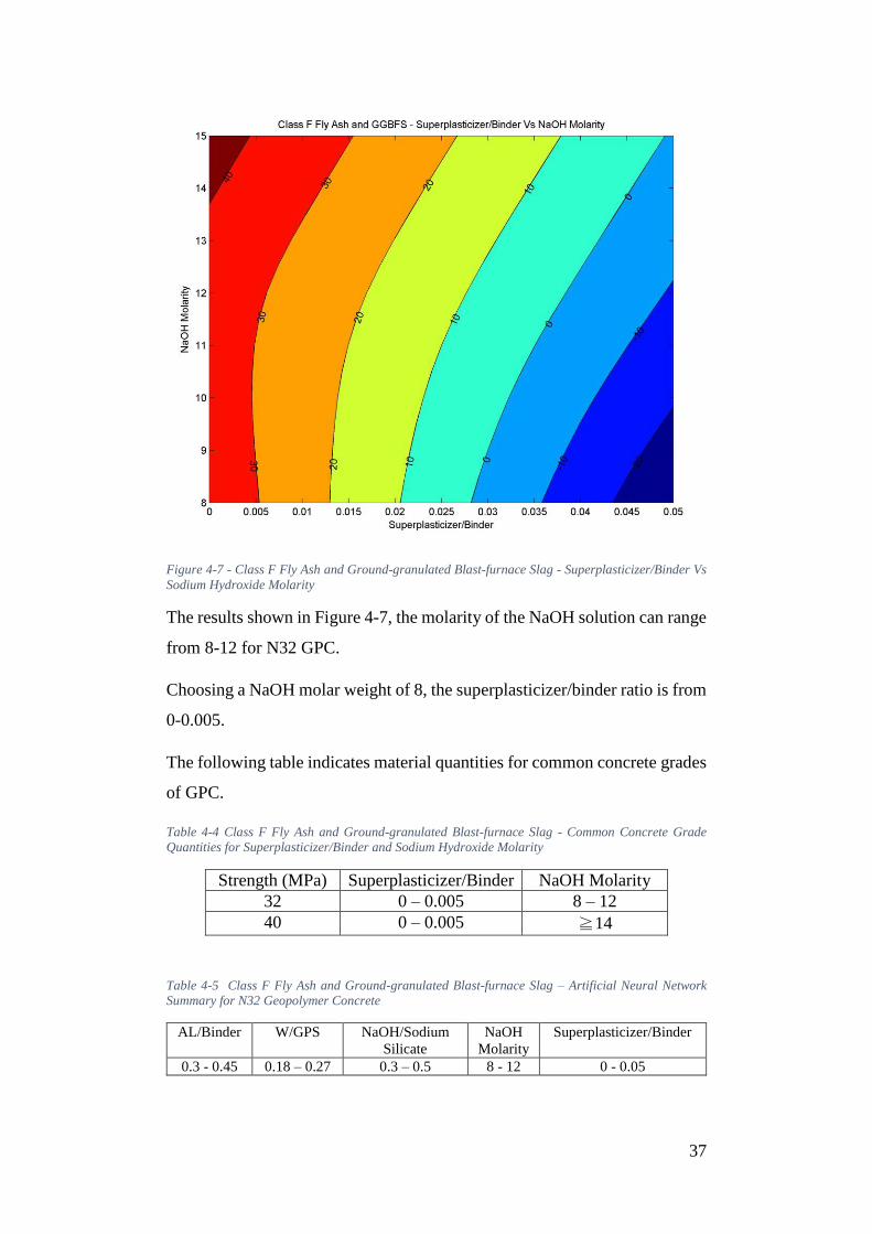
Figure 4-7 - Class F Fly Ash and Ground-granulated Blast-furnace Slag - Superplasticizer/Binder Vs

Sodium Hydroxide Molarity

The results shown in Figure 4-7, the molarity of the NaOH solution can range

from 8-12 for N32 GPC.

Choosing a NaOH molar weight of 8, the superplasticizer/binder ratio is from

0-0.005.


of GPC.


Quantities for Superplasticizer/Binder and Sodium Hydroxide Molarity

Strength (MPa) Superplasticizer/Binder NaOH Molarity

32 0 – 0.005 8 – 12

40 0 – 0.005 ≧14

Table 4-5 Class F Fly Ash and Ground-granulated Blast-furnace Slag – Artificial Neural Network

Summary for N32 Geopolymer Concrete

AL/Binder W/GPS NaOH/Sodium

Silicate

NaOH

Molarity

Superplasticizer/Binder

0.3 - 0.45 0.18 – 0.27 0.3 – 0.5 8 - 12 0 - 0.05

38

This will be the only mixture tested for compressive strength due to time and

material constraint. Six cylinders of 100mm diameter x 200mm high will be

created to test for compressive strength of N32 GPC. This equates to

approximately 0.0094m3 of GPC, with some extra for spillage. Based on a

concrete density of 2500kg/m3, the weight of concrete required is

approximately 35kg.

As the aggregates are based on OPC quantities, the percentages of course and

fine aggregates will be the same as that for the Class F mix. Therefore, the

total weight of aggregates is 28kg, with fine sands equalling 9.8kg of that.

From the database, the average fly ash/total weight ratio is 0.13, whilst the

average slag/total weight ratio is 0.06. Therefore, 4.55kg of Class F FA and

2.1kg of GGBFS are required for this mix.

For the alkaline solution, the ratio of AL/Binder will be taken as 0.4. This

would indicate a quantity of alkaline solution to be 2.66kg. Taking the

NaOH/Sodium Silicate ratio as 0.4, this would indicate quantities:

NaOH solution = 1.064kg

Sodium Silicate solution = 1.596kg

Based on a W/GPS ratio of 0.25 and average percentages from the database:

55.9% water for hydroxide solution = 0.595L of water

57.9% water for silicate solution = 0.924L of water

Extra Water = Approximately 0.43L

Total water required = 1.95 litres

For the Superplasticizer, the super/binder ratio of 0.0025 will be used.

Therefore, 0.02kg of Superplasticizer may be required.

39

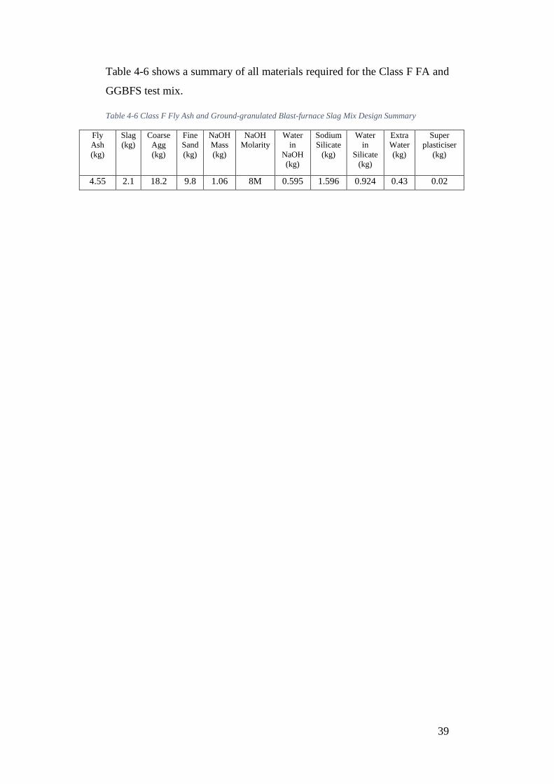
Table 4-6 shows a summary of all materials required for the Class F FA and

GGBFS test mix.

Table 4-6 Class F Fly Ash and Ground-granulated Blast-furnace Slag Mix Design Summary

Fly

Ash

(kg)

Slag

(kg)

Coarse

Agg

(kg)

Fine

Sand

(kg)

NaOH

Mass

(kg)

NaOH

Molarity

Water

in

NaOH

(kg)

Sodium

Silicate

(kg)

Water

in

Silicate

(kg)

Extra

Water

(kg)

Super

plasticiser

(kg)

4.55 2.1 18.2 9.8 1.06 8M 0.595 1.596 0.924 0.43 0.02

40

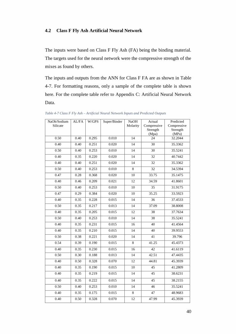
4.2 Class F Fly Ash Artificial Neural Network

The inputs were based on Class F Fly Ash (FA) being the binding material.

The targets used for the neural network were the compressive strength of the

mixes as found by others.

The inputs and outputs from the ANN for Class F FA are as shown in Table

4-7. For formatting reasons, only a sample of the complete table is shown

here. For the complete table refer to Appendix C: Artificial Neural Network

Data.

Table 4-7 Class F Fly Ash – Artificial Neural Network Inputs and Predicted Outputs

NaOh/Sodium

Silicate

AL/FA W/GPS Super/Binder NaOH

Molarity

Actual

Compressive

Strength

(Mpa)

Predicted

Compressive

Strength

(MPa)

0.50 0.40 0.295 0.010 14 24 32.2044

0.40 0.40 0.251 0.020 14 30 35.3362

0.50 0.40 0.253 0.010 14 30 35.5241

0.40 0.35 0.220 0.020 14 32 40.7442

0.40 0.40 0.251 0.020 14 32 35.3362

0.50 0.40 0.253 0.010 8 32 34.5394

0.47 0.28 0.368 0.020 10 33.75 35.1475

0.40 0.46 0.209 0.021 12 34.59 41.8601

0.50 0.40 0.253 0.010 10 35 31.9175

0.47 0.29 0.384 0.020 10 35.25 33.5923

0.40 0.35 0.228 0.015 14 36 37.4533

0.50 0.35 0.217 0.013 14 37.09 38.8008

0.40 0.35 0.205 0.015 12 38 37.7634

0.50 0.40 0.253 0.010 14 38 35.5241

0.40 0.35 0.231 0.015 16 40 41.4564

0.40 0.35 0.210 0.015 14 40 39.9553

0.50 0.38 0.221 0.020 14 41 39.796

0.54 0.39 0.190 0.015 8 41.25 45.4373

0.40 0.35 0.230 0.015 16 42 41.6119

0.50 0.30 0.188 0.013 14 42.51 47.4435

0.40 0.50 0.328 0.070 12 44.81 45.3939

0.40 0.35 0.190 0.015 10 45 41.2809

0.40 0.35 0.219 0.015 14 45 38.6231

0.40 0.35 0.222 0.015 14 45 38.2155

0.50 0.40 0.253 0.010 14 46 35.5241

0.40 0.35 0.175 0.015 8 47 48.9683

0.40 0.50 0.328 0.070 12 47.99 45.3939

41

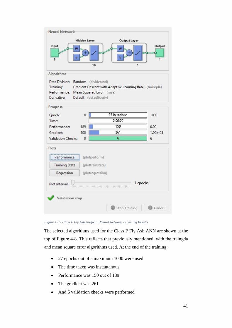
Figure 4-8 - Class F Fly Ash Artificial Neural Network - Training Results

The selected algorithms used for the Class F Fly Ash ANN are shown at the

top of Figure 4-8. This reflects that previously mentioned, with the traingda

and mean square error algorithms used. At the end of the training:


The time taken was instantanous

Performance was 150 out of 189

The gradient was 261


42

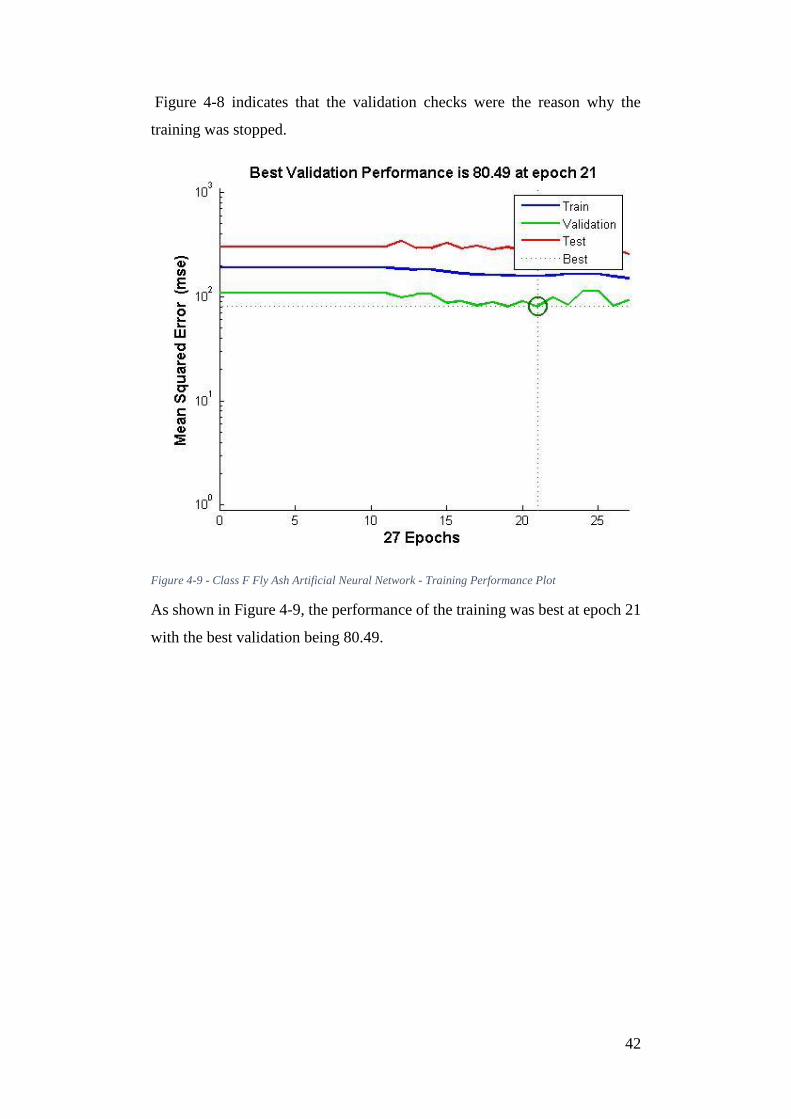
Figure 4-8 indicates that the validation checks were the reason why the

training was stopped.

Figure 4-9 - Class F Fly Ash Artificial Neural Network - Training Performance Plot

As shown in Figure 4-9, the performance of the training was best at epoch 21

with the best validation being 80.49.

43

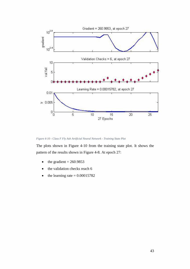
Figure 4-10 - Class F Fly Ash Artificial Neural Network - Training State Plot

The plots shown in Figure 4-10 from the training state plot. It shows the

pattern of the results shown in Figure 4-8. At epoch 27:




44

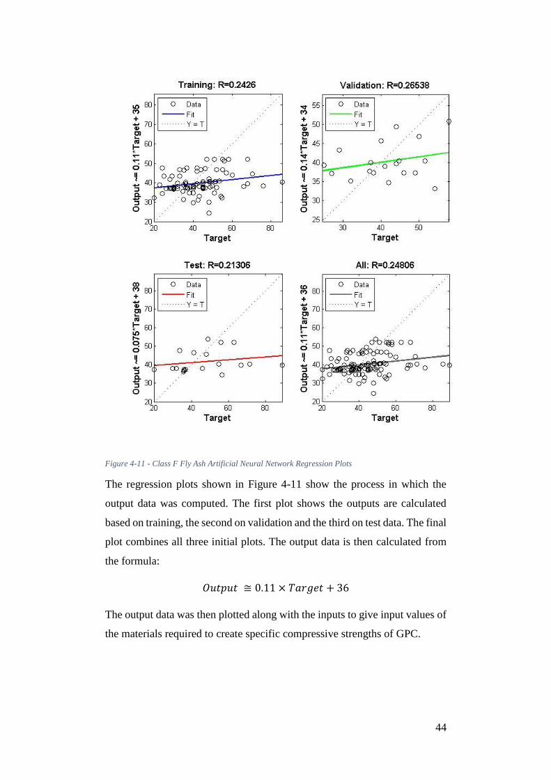
Figure 4-11 - Class F Fly Ash Artificial Neural Network Regression Plots




plot combines all three initial plots. The output data is then calculated from

the formula:

𝑂𝑢𝑡𝑝𝑢𝑡 ≅ 0.11 × 𝑇𝑎𝑟𝑔𝑒𝑡 + 36



45

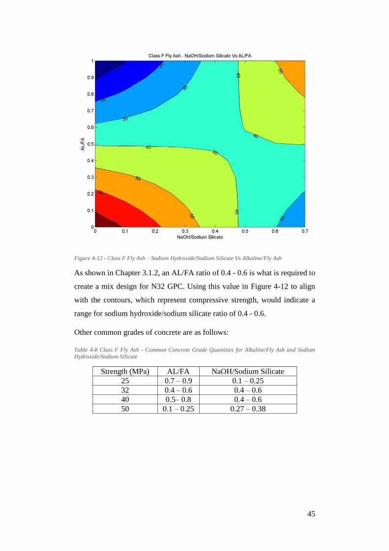
Figure 4-12 - Class F Fly Ash – Sodium Hydroxide/Sodium Silicate Vs Alkaline/Fly Ash

As shown in Chapter 3.1.2, an AL/FA ratio of 0.4 - 0.6 is what is required to

create a mix design for N32 GPC. Using this value in Figure 4-12 to align

with the contours, which represent compressive strength, would indicate a

range for sodium hydroxide/sodium silicate ratio of 0.4 - 0.6.

Other common grades of concrete are as follows:

Table 4-8 Class F Fly Ash - Common Concrete Grade Quantities for Alkaline/Fly Ash and Sodium

Hydroxide/Sodium Silicate

Strength (MPa) AL/FA NaOH/Sodium Silicate

25 0.7 – 0.9 0.1 – 0.25

32 0.4 – 0.6 0.4 – 0.6

40 0.5– 0.8 0.4 – 0.6

50 0.1 – 0.25 0.27 – 0.38

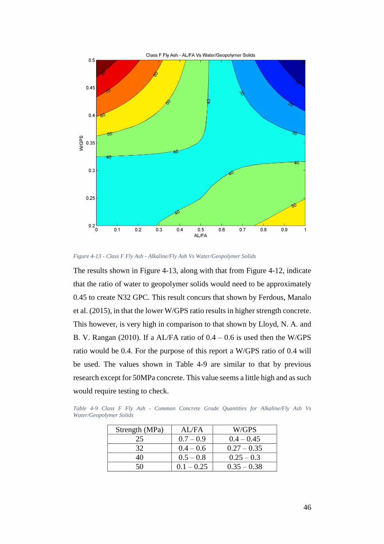
46

Figure 4-13 - Class F Fly Ash - Alkaline/Fly Ash Vs Water/Geopolymer Solids

The results shown in Figure 4-13, along with that from Figure 4-12, indicate

that the ratio of water to geopolymer solids would need to be approximately

0.45 to create N32 GPC. This result concurs that shown by Ferdous, Manalo

et al. (2015), in that the lower W/GPS ratio results in higher strength concrete.

This however, is very high in comparison to that shown by Lloyd, N. A. and

B. V. Rangan (2010). If a AL/FA ratio of 0.4 – 0.6 is used then the W/GPS

ratio would be 0.4. For the purpose of this report a W/GPS ratio of 0.4 will

be used. The values shown in Table 4-9 are similar to that by previous

research except for 50MPa concrete. This value seems a little high and as such

would require testing to check.

Table 4-9 Class F Fly Ash - Common Concrete Grade Quantities for Alkaline/Fly Ash Vs


Strength (MPa) AL/FA W/GPS

25 0.7 – 0.9 0.4 – 0.45

32 0.4 – 0.6 0.27 – 0.35

40 0.5 – 0.8 0.25 – 0.3

50 0.1 – 0.25 0.35 – 0.38

47

Figure 4-14 - Class F Fly Ash - Superplasticizer/Binder Ratio Vs Sodium Hydroxide Molarity

Figure 4-14 shows the relationship between superplasticizer/binder ratio and

the molarity of the NaOH solution. It is evident that as the molarity of the

NaOH solution increases, so too does the ratio of the superplasticizer to

binder. For N32 concrete, NaOH molarity range of 12–14 with

superplasticizer/binder ratio range of 0.04 – 0.1.

Table 4-10 Class F Fly Ash - Common Concrete Grade Quantities for Superplasticizer/Binder and



32 0.04 – 0.1 12 - 14

40 0.02 – 0.1 9 - 12

50 0.035 – 0.06 8 - 10

Table 4-11 Class F Fly Ash Artificial Neural Network Summary for N32 Geopolymer Concrete

AL/FA W/GPS NaOH/Sodium

Silicate

NaOH

Molarity


0.4 - 0.6 0.27 – 0.35 0.4 – 0.6 12 – 14 0.04 – 0.1

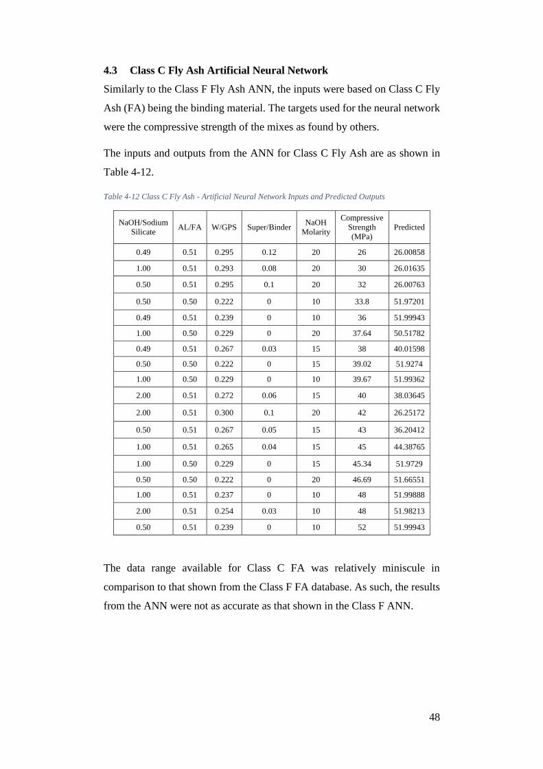
48

4.3 Class C Fly Ash Artificial Neural Network

Similarly to the Class F Fly Ash ANN, the inputs were based on Class C Fly

Ash (FA) being the binding material. The targets used for the neural network

were the compressive strength of the mixes as found by others.

The inputs and outputs from the ANN for Class C Fly Ash are as shown in

Table 4-12.

Table 4-12 Class C Fly Ash - Artificial Neural Network Inputs and Predicted Outputs

NaOH/Sodium

Silicate AL/FA W/GPS Super/Binder

NaOH

Molarity

Compressive

Strength

(MPa)

Predicted

0.49 0.51 0.295 0.12 20 26 26.00858

1.00 0.51 0.293 0.08 20 30 26.01635

0.50 0.51 0.295 0.1 20 32 26.00763

0.50 0.50 0.222 0 10 33.8 51.97201

0.49 0.51 0.239 0 10 36 51.99943

1.00 0.50 0.229 0 20 37.64 50.51782

0.49 0.51 0.267 0.03 15 38 40.01598

0.50 0.50 0.222 0 15 39.02 51.9274

1.00 0.50 0.229 0 10 39.67 51.99362

2.00 0.51 0.272 0.06 15 40 38.03645

2.00 0.51 0.300 0.1 20 42 26.25172

0.50 0.51 0.267 0.05 15 43 36.20412

1.00 0.51 0.265 0.04 15 45 44.38765

1.00 0.50 0.229 0 15 45.34 51.9729

0.50 0.50 0.222 0 20 46.69 51.66551

1.00 0.51 0.237 0 10 48 51.99888

2.00 0.51 0.254 0.03 10 48 51.98213

0.50 0.51 0.239 0 10 52 51.99943

The data range available for Class C FA was relatively miniscule in

comparison to that shown from the Class F FA database. As such, the results

from the ANN were not as accurate as that shown in the Class F ANN.

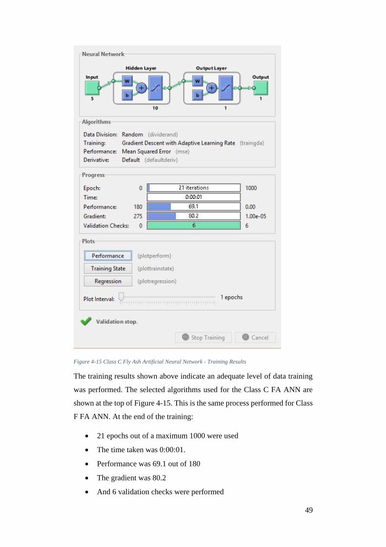
49

Figure 4-15 Class C Fly Ash Artificial Neural Network - Training Results

The training results shown above indicate an adequate level of data training

was performed. The selected algorithms used for the Class C FA ANN are

shown at the top of Figure 4-15. This is the same process performed for Class

F FA ANN. At the end of the training:




The gradient was 80.2


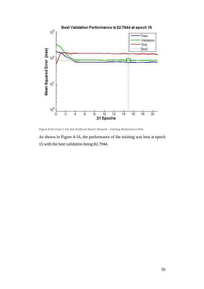
50

Figure 4-16 Class C Fly Ash Artificial Neural Network - Training Performance Plot

As shown in Figure 4-16, the performance of the training was best at epoch

15 with the best validation being 82.7944.

51

Figure 4-17 Class C Fly Ash Artificial Neural Network - Training State Plot

The plots shown in Figure 4-17 from the training state plot. It shows the





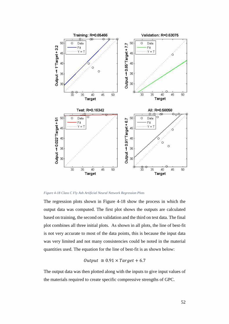
52

Figure 4-18 Class C Fly Ash Artificial Neural Network Regression Plots




plot combines all three initial plots. As shown in all plots, the line of best-fit

is not very accurate to most of the data points, this is because the input data

was very limited and not many consistencies could be noted in the material

quantities used. The equation for the line of best-fit is as shown below:

𝑂𝑢𝑡𝑝𝑢𝑡 ≅ 0.91 × 𝑇𝑎𝑟𝑔𝑒𝑡 + 6.7



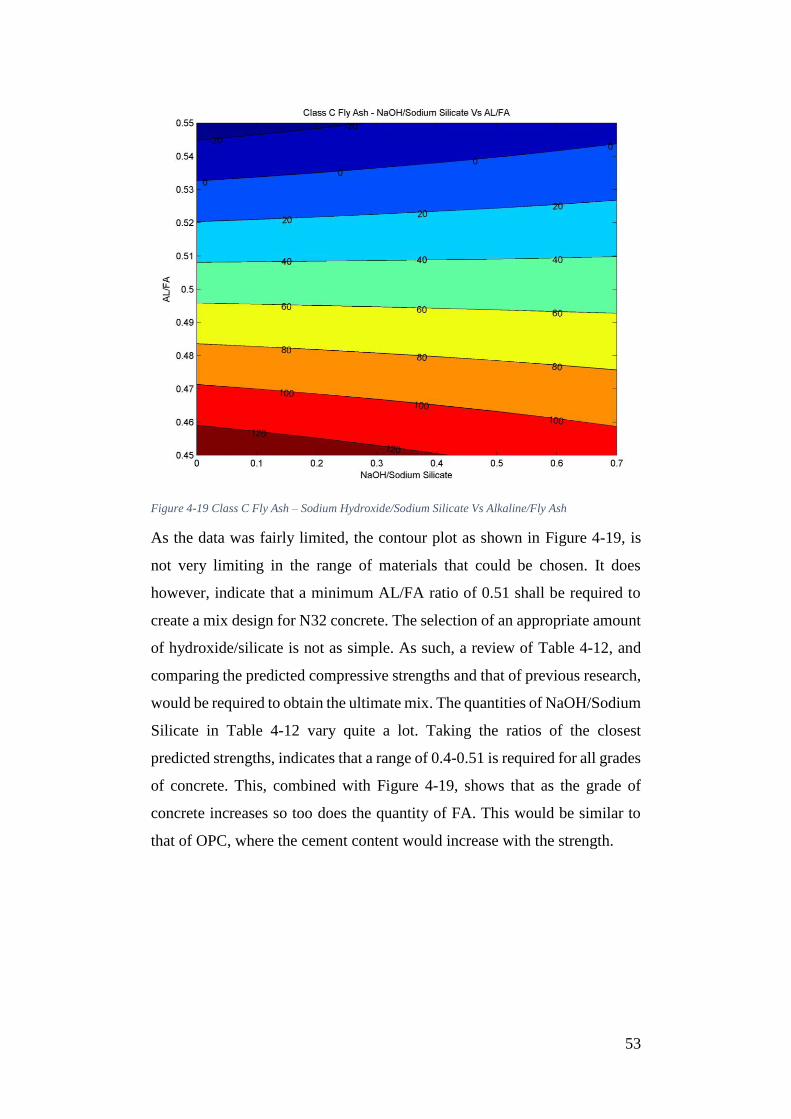
53

Figure 4-19 Class C Fly Ash – Sodium Hydroxide/Sodium Silicate Vs Alkaline/Fly Ash

As the data was fairly limited, the contour plot as shown in Figure 4-19, is

not very limiting in the range of materials that could be chosen. It does

however, indicate that a minimum AL/FA ratio of 0.51 shall be required to

create a mix design for N32 concrete. The selection of an appropriate amount

of hydroxide/silicate is not as simple. As such, a review of Table 4-12, and

comparing the predicted compressive strengths and that of previous research,

would be required to obtain the ultimate mix. The quantities of NaOH/Sodium

Silicate in Table 4-12 vary quite a lot. Taking the ratios of the closest

predicted strengths, indicates that a range of 0.4-0.51 is required for all grades

of concrete. This, combined with Figure 4-19, shows that as the grade of

concrete increases so too does the quantity of FA. This would be similar to

that of OPC, where the cement content would increase with the strength.

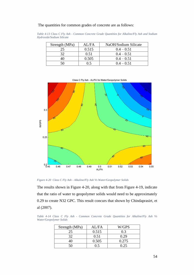
54

The quantities for common grades of concrete are as follows:

Table 4-13 Class C Fly Ash - Common Concrete Grade Quantities for Alkaline/Fly Ash and Sodium

Hydroxide/Sodium Silicate

Strength (MPa) AL/FA NaOH/Sodium Silicate

25 0.515 0.4 – 0.51

32 0.51 0.4 – 0.51

40 0.505 0.4 – 0.51

50 0.5 0.4 – 0.51

Figure 4-20 Class C Fly Ash - Alkaline/Fly Ash Vs Water/Geopolymer Solids



0.29 to create N32 GPC. This result concurs that shown by Chindaprasirt, et

al (2007).

Table 4-14 Class C Fly Ash - Common Concrete Grade Quantities for Alkaline/Fly Ash Vs


Strength (MPa) AL/FA W/GPS

25 0.515 0.3

32 0.51 0.29

40 0.505 0.275

50 0.5 0.25

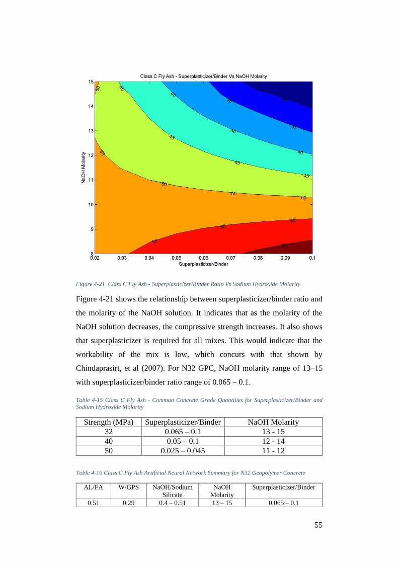
55

Figure 4-21 Class C Fly Ash - Superplasticizer/Binder Ratio Vs Sodium Hydroxide Molarity

Figure 4-21 shows the relationship between superplasticizer/binder ratio and

the molarity of the NaOH solution. It indicates that as the molarity of the

NaOH solution decreases, the compressive strength increases. It also shows

that superplasticizer is required for all mixes. This would indicate that the

workability of the mix is low, which concurs with that shown by

Chindaprasirt, et al (2007). For N32 GPC, NaOH molarity range of 13–15

with superplasticizer/binder ratio range of 0.065 – 0.1.

Table 4-15 Class C Fly Ash - Common Concrete Grade Quantities for Superplasticizer/Binder and



32 0.065 – 0.1 13 - 15

40 0.05 – 0.1 12 - 14

50 0.025 – 0.045 11 - 12

Table 4-16 Class C Fly Ash Artificial Neural Network Summary for N32 Geopolymer Concrete

AL/FA W/GPS NaOH/Sodium

Silicate

NaOH

Molarity


0.51 0.29 0.4 – 0.51 13 – 15 0.065 – 0.1

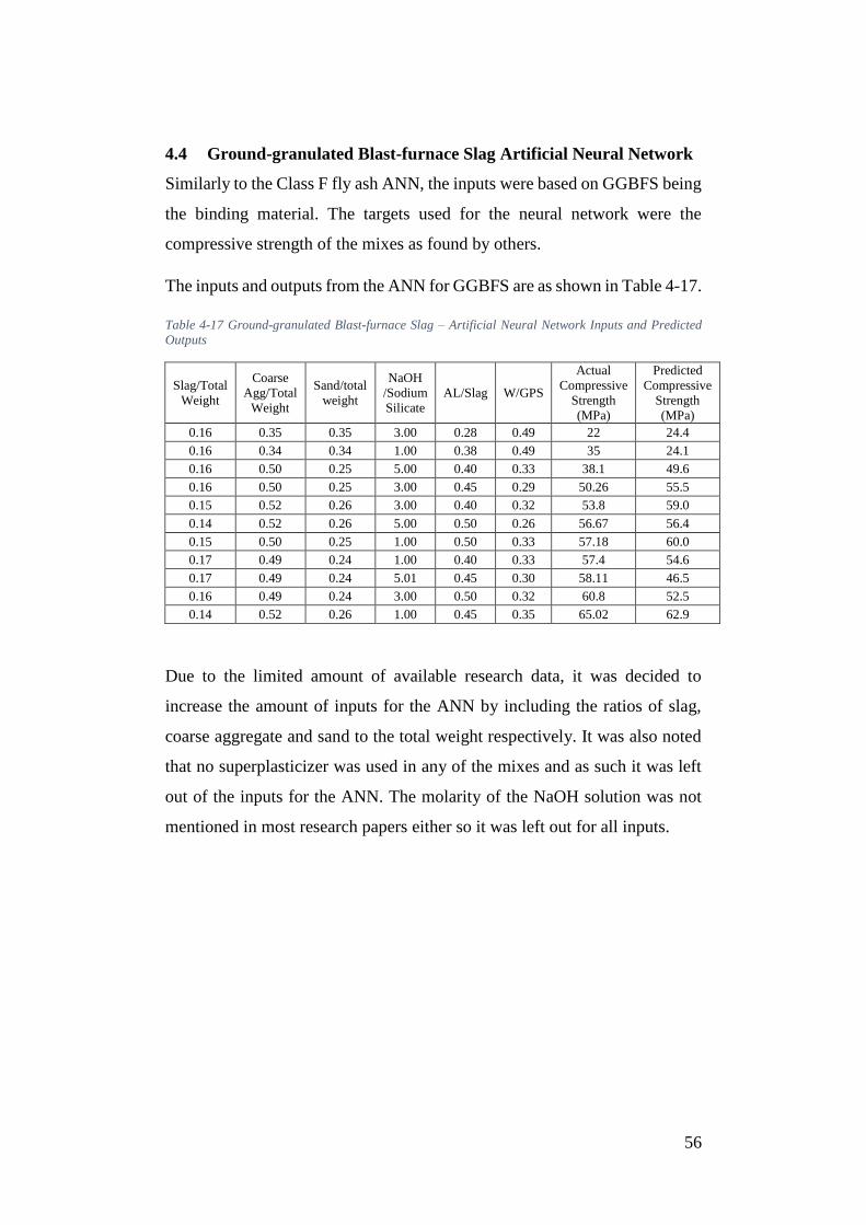
56

4.4 Ground-granulated Blast-furnace Slag Artificial Neural Network

Similarly to the Class F fly ash ANN, the inputs were based on GGBFS being

the binding material. The targets used for the neural network were the

compressive strength of the mixes as found by others.

The inputs and outputs from the ANN for GGBFS are as shown in Table 4-17.

Table 4-17 Ground-granulated Blast-furnace Slag – Artificial Neural Network Inputs and Predicted

Outputs

Slag/Total

Weight

Coarse

Agg/Total

Weight

Sand/total

weight

NaOH

/Sodium

Silicate

AL/Slag W/GPS

Actual

Compressive

Strength

(MPa)

Predicted

Compressive

Strength

(MPa)

0.16 0.35 0.35 3.00 0.28 0.49 22 24.4

0.16 0.34 0.34 1.00 0.38 0.49 35 24.1

0.16 0.50 0.25 5.00 0.40 0.33 38.1 49.6

0.16 0.50 0.25 3.00 0.45 0.29 50.26 55.5

0.15 0.52 0.26 3.00 0.40 0.32 53.8 59.0

0.14 0.52 0.26 5.00 0.50 0.26 56.67 56.4

0.15 0.50 0.25 1.00 0.50 0.33 57.18 60.0

0.17 0.49 0.24 1.00 0.40 0.33 57.4 54.6

0.17 0.49 0.24 5.01 0.45 0.30 58.11 46.5

0.16 0.49 0.24 3.00 0.50 0.32 60.8 52.5

0.14 0.52 0.26 1.00 0.45 0.35 65.02 62.9

Due to the limited amount of available research data, it was decided to

increase the amount of inputs for the ANN by including the ratios of slag,

coarse aggregate and sand to the total weight respectively. It was also noted

that no superplasticizer was used in any of the mixes and as such it was left

out of the inputs for the ANN. The molarity of the NaOH solution was not

mentioned in most research papers either so it was left out for all inputs.

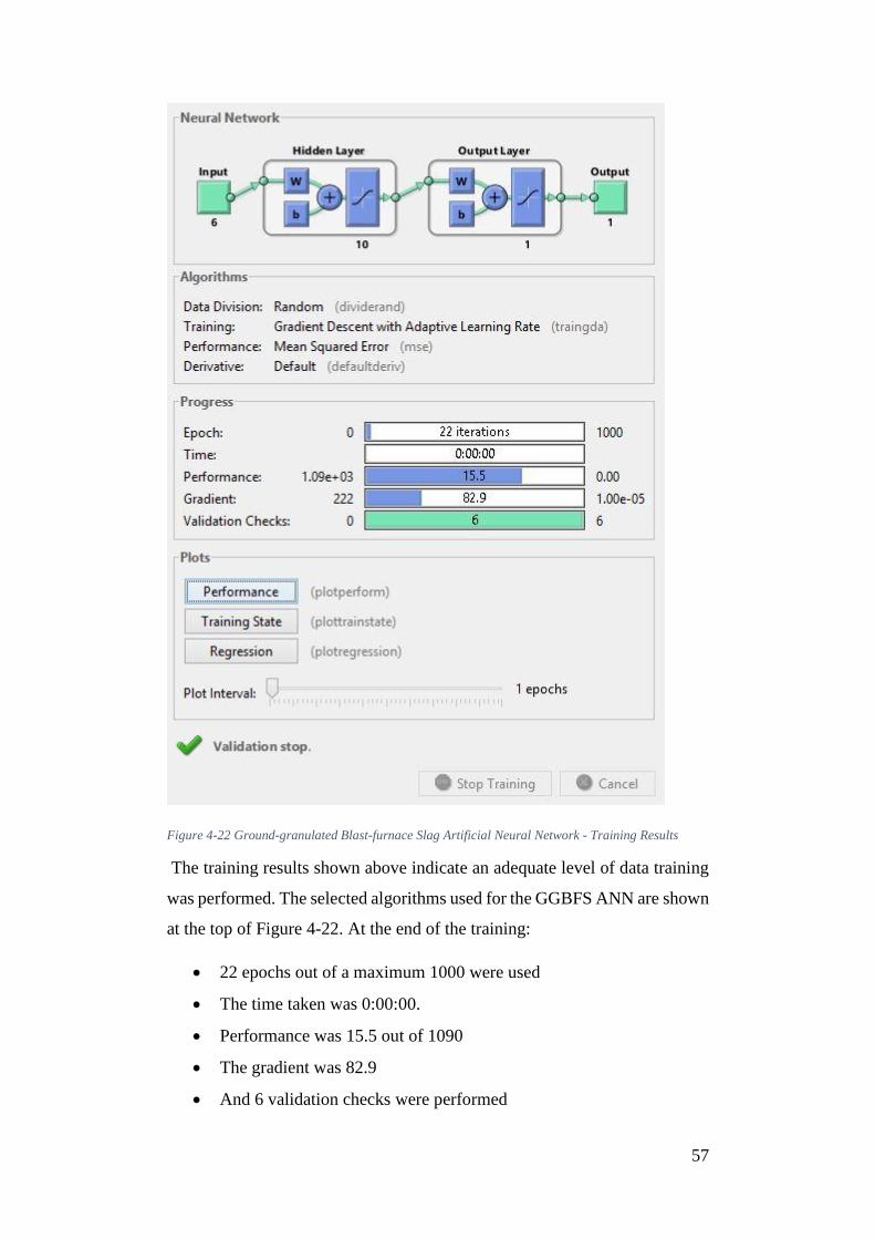
57

Figure 4-22 Ground-granulated Blast-furnace Slag Artificial Neural Network - Training Results

The training results shown above indicate an adequate level of data training

was performed. The selected algorithms used for the GGBFS ANN are shown

at the top of Figure 4-22. At the end of the training:




The gradient was 82.9


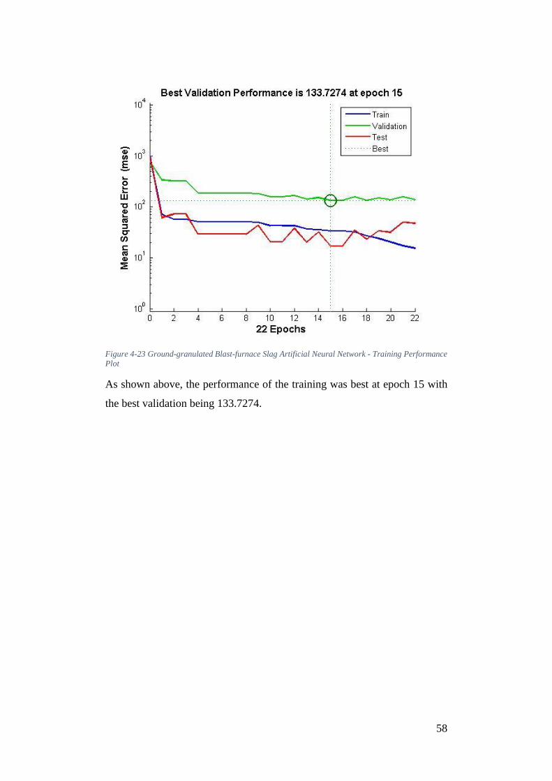
58

Figure 4-23 Ground-granulated Blast-furnace Slag Artificial Neural Network - Training Performance

Plot

As shown above, the performance of the training was best at epoch 15 with

the best validation being 133.7274.

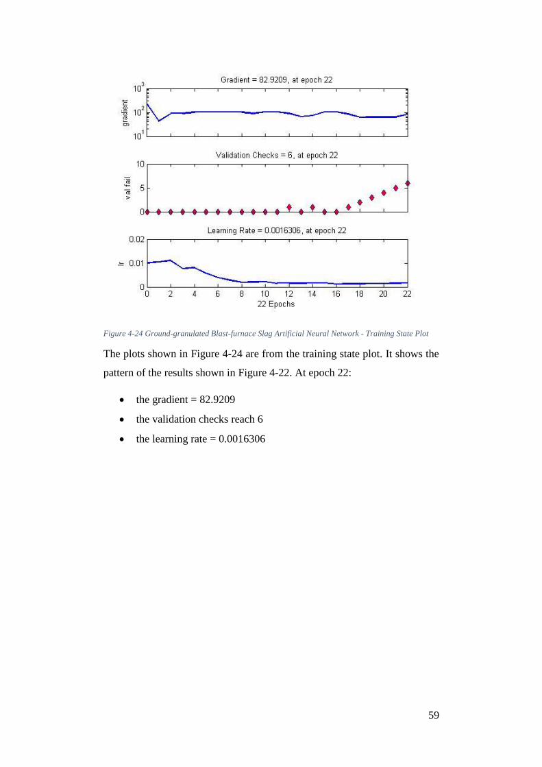
59

Figure 4-24 Ground-granulated Blast-furnace Slag Artificial Neural Network - Training State Plot

The plots shown in Figure 4-24 are from the training state plot. It shows the





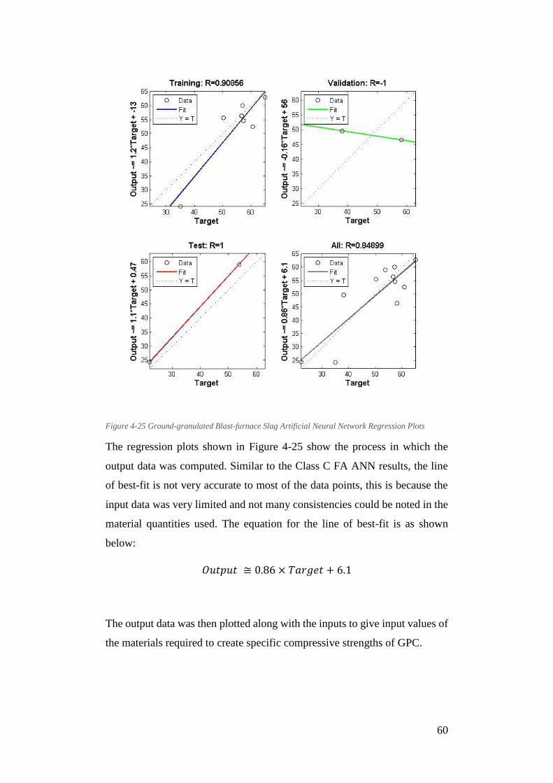
60

Figure 4-25 Ground-granulated Blast-furnace Slag Artificial Neural Network Regression Plots


output data was computed. Similar to the Class C FA ANN results, the line

of best-fit is not very accurate to most of the data points, this is because the

input data was very limited and not many consistencies could be noted in the

material quantities used. The equation for the line of best-fit is as shown

below:

𝑂𝑢𝑡𝑝𝑢𝑡 ≅ 0.86 × 𝑇𝑎𝑟𝑔𝑒𝑡 + 6.1



61

Figure 4-26 Ground-granulated Blast-furnace Slag – Sodium Hydroxide/Sodium Silicate Vs

Alkaline/Slag

From Figure 4-26, the ratios of AL/slag and NaOH/Sodium silicate can be

determined for standard concrete grades.

The quantities for common grades of concrete are as follows:

Table 4-18 Ground-granulated Blast-furnace Slag - Common Concrete Grade Quantities for

Alkaline/Slag and Sodium Hydroxide/Sodium Silicate

Strength (MPa) AL/Slag NaOH/Sodium Silicate

32 0.32 0.4-0.7

40 0.38 0.4-0.7

50 0.42 0.4-0.7

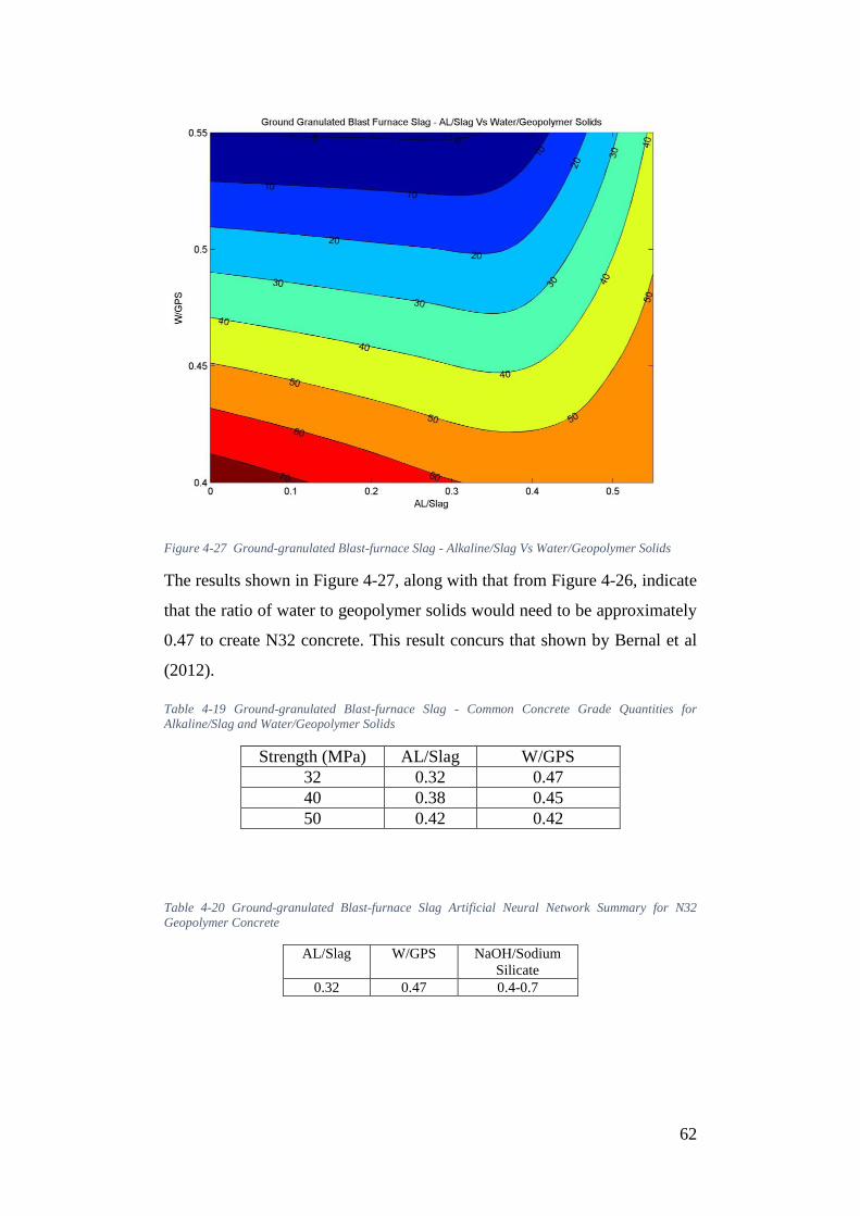
62

Figure 4-27 Ground-granulated Blast-furnace Slag - Alkaline/Slag Vs Water/Geopolymer Solids



0.47 to create N32 concrete. This result concurs that shown by Bernal et al

(2012).

Table 4-19 Ground-granulated Blast-furnace Slag - Common Concrete Grade Quantities for

Alkaline/Slag and Water/Geopolymer Solids

Strength (MPa) AL/Slag W/GPS

32 0.32 0.47

40 0.38 0.45

50 0.42 0.42

Table 4-20 Ground-granulated Blast-furnace Slag Artificial Neural Network Summary for N32

Geopolymer Concrete

AL/Slag W/GPS NaOH/Sodium

Silicate

0.32 0.47 0.4-0.7

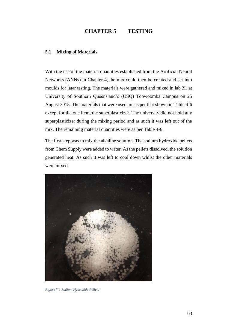
63

CHAPTER 5 TESTING

5.1 Mixing of Materials

With the use of the material quantities established from the Artificial Neural

Networks (ANNs) in Chapter 4, the mix could then be created and set into

moulds for later testing. The materials were gathered and mixed in lab Z1 at

University of Southern Queensland’s (USQ) Toowoomba Campus on 25

August 2015. The materials that were used are as per that shown in Table 4-6

except for the one item, the superplasticizer. The university did not hold any

superplasticizer during the mixing period and as such it was left out of the

mix. The remaining material quantities were as per Table 4-6.

The first step was to mix the alkaline solution. The sodium hydroxide pellets

from Chem Supply were added to water. As the pellets dissolved, the solution

generated heat. As such it was left to cool down whilst the other materials

were mixed.

Figure 5-1 Sodium Hydroxide Pellets

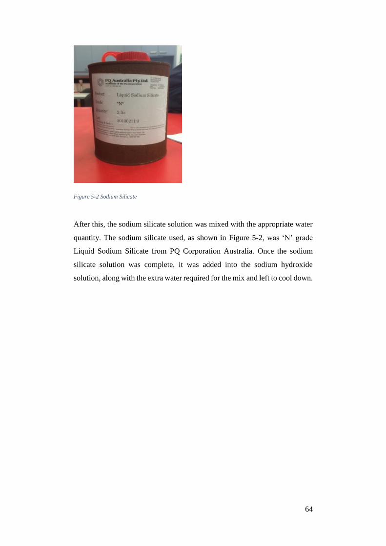
64

Figure 5-2 Sodium Silicate

After this, the sodium silicate solution was mixed with the appropriate water

quantity. The sodium silicate used, as shown in Figure 5-2, was ‘N’ grade

Liquid Sodium Silicate from PQ Corporation Australia. Once the sodium

silicate solution was complete, it was added into the sodium hydroxide

solution, along with the extra water required for the mix and left to cool down.

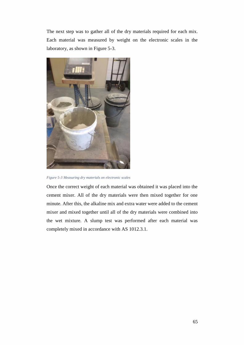
65

The next step was to gather all of the dry materials required for each mix.

Each material was measured by weight on the electronic scales in the

laboratory, as shown in Figure 5-3.

Figure 5-3 Measuring dry materials on electronic scales

Once the correct weight of each material was obtained it was placed into the

cement mixer. All of the dry materials were then mixed together for one

minute. After this, the alkaline mix and extra water were added to the cement

mixer and mixed together until all of the dry materials were combined into

the wet mixture. A slump test was performed after each material was

completely mixed in accordance with AS 1012.3.1.

66

Figure 5-4 Slump Test Cone (AS1012.3.1)

The cone was filled in three equal layers with each layer rodded 25 times for

compaction reasons. The slump for the Class F Fly Ash (FA) and Ground-

granulated Blast-furnace Slag (GGBFS) mix was 160mm.

This slump value is very high in comparison to Ordinary Portland Cement

(OPC) mixes but are fairly similar to that shown by Hardjito (2005).

After the slump test was performed, the mix was then placed into moulds.

This was done so by filling the mould half way, rodding 25 times with an R24

bar, then filling to the top and rodding again 25 times. Figure 5-5 depicts the

compaction by rodding with the R24 bar.

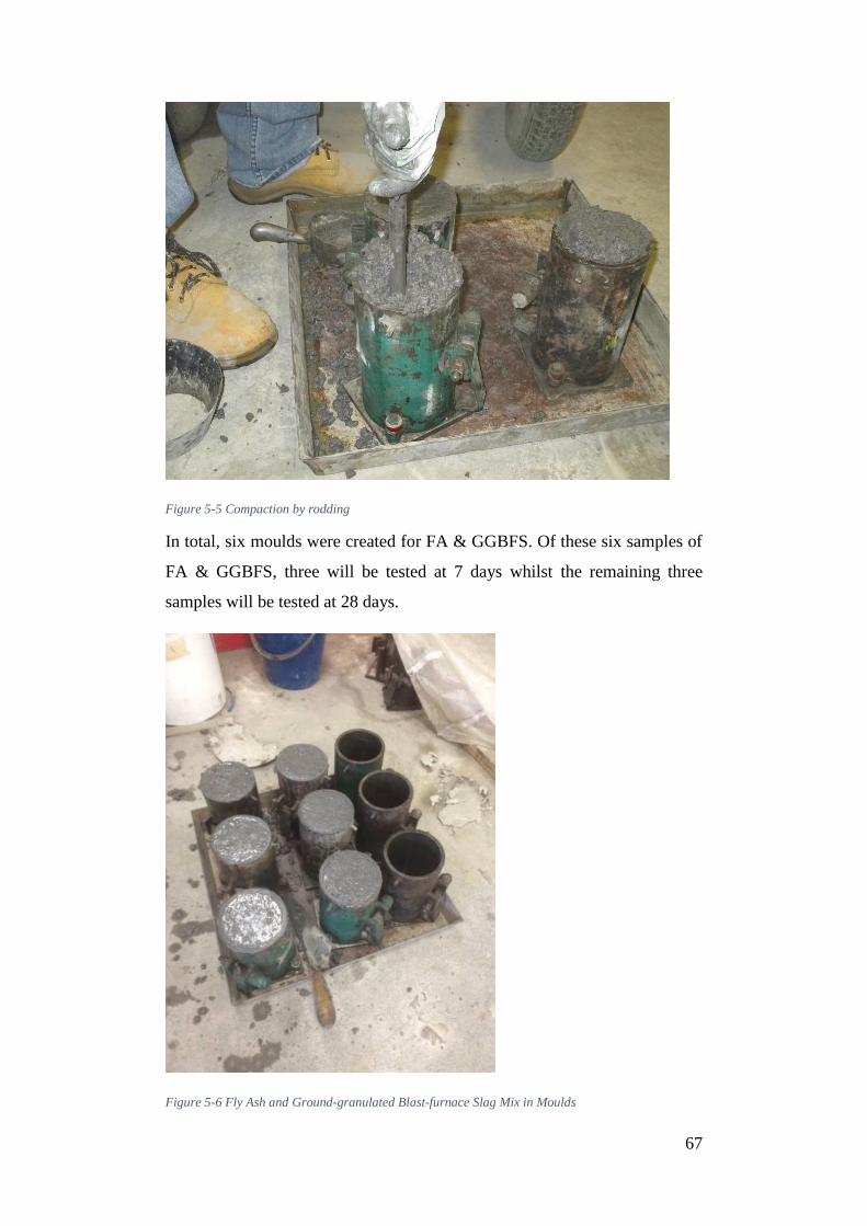
67

Figure 5-5 Compaction by rodding

In total, six moulds were created for FA & GGBFS. Of these six samples of

FA & GGBFS, three will be tested at 7 days whilst the remaining three

samples will be tested at 28 days.

Figure 5-6 Fly Ash and Ground-granulated Blast-furnace Slag Mix in Moulds

68

Once the mould was completely full, the top was finished with a small trowl

and then placed into the curing room for 36 hours at 27° as per AS1012.8.1-

2014. The samples were removed from the moulds after 24 hours, to free them

up for other students. The samples were then placed back into the curing room

for the rest of the 36 hour curing period. After the 36 hours had passed, the

samples were removed from the curing room and left to cure at room

temperature for the remainder of the waiting period until test day.

69

5.2 Testing Procedure

Seven days after the moulds were set, 3 cylinders of FA and GGBFS were

tested for compressive strength in accordance with AS1012.9-2014 Methods

of testing concrete, Method 9: Compressive strength tests. These tests were

performed in lab Z1 at USQ’s Toowoomba Campus on 2 September 2015.

Figure 5-7 Sample setup for Compressive Strength Test

Figure 5-7 shows the sample set into the machine ready for testing. The

sample was locked in place with a rubber based cap which was placed on top

of the sample. The cap then slotted into the machine’s top plate and lowered

into position so that the base was resting on the bottom plate. The impact

machine was then set to apply a force equivalent to 20 +/- 2MPa compressive

stress per minute until there is no more increase in force, as per AS 1012.9-

2014. The maximum force applied to the sample was then noted from the

display on the impact machine.

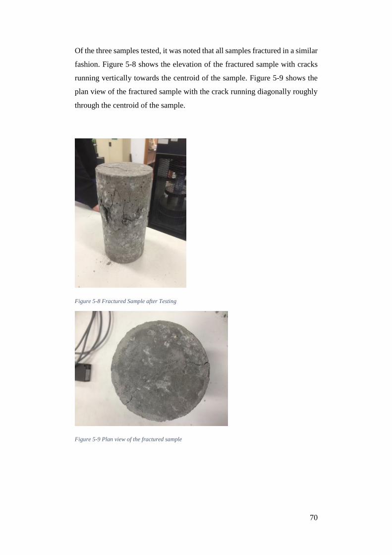
70

Of the three samples tested, it was noted that all samples fractured in a similar

fashion. Figure 5-8 shows the elevation of the fractured sample with cracks

running vertically towards the centroid of the sample. Figure 5-9 shows the

plan view of the fractured sample with the crack running diagonally roughly

through the centroid of the sample.

Figure 5-8 Fractured Sample after Testing

Figure 5-9 Plan view of the fractured sample

71

CHAPTER 6 RESULTS AND DISCUSSION

Table 6-1 Compressive Test Results at 7 days

Sample type Age

Days

Initial

Curing

Hours

Ambient

Curing

Days

Height

(mm)

Diameter

(mm)

Force (kN) Strength

(MPa)

1 FA + GGBFS 7 28 6 200 100 111.7 14.2

2 FA + GGBFS 7 28 6 200 100 106.3 14.1

3 FA + GGBFS 7 28 6 200 100 106.1 14.1

The test results shown in Table 6-1 indicate a 7 day force required for fracture

of the specimen of approximately 106kN. This would translate to a

compressive strength of 14MPa. According to AS1379-2007 - Specification

and supply of concrete, this would indicate a concrete grade of roughly

28MPa at 28 days, as shown in Table 6-2. This table is based on OPC and the

results of the 28 day compression tests will be required to compare these

values.

Table 6-2 Mean 7 day Compressive Strengths (AS1379-2007)

Figure 6-1 Compressive Strengths over time for curing at ambient conditions (Rangan 2006)

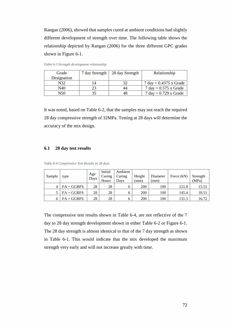
72

Rangan (2006), showed that samples cured at ambient conditions had slightly

different development of strength over time. The following table shows the

relationship depicted by Rangan (2006) for the three different GPC grades

shown in Figure 6-1.

Table 6-3 Strength development relationship

Grade

Designation

7 day Strength 28 day Strength Relationship

N32 14 32 7 day = 0.4375 x Grade

N40 23 44 7 day = 0.575 x Grade

N50 35 48 7 day = 0.729 x Grade

It was noted, based on Table 6-2, that the samples may not reach the required

28 day compressive strength of 32MPa. Testing at 28 days will determine the

accuracy of the mix design.

6.1 28 day test results

Table 6-4 Compressive Test Results at 28 days

Sample type Age

Days

Initial

Curing

Hours

Ambient

Curing

Days

Height

(mm)

Diameter

(mm)

Force (kN) Strength

(MPa)

4 FA + GGBFS 28 28 6 200 100 121.8 15.51

5 FA + GGBFS 28 28 6 200 100 145.4 18.51

6 FA + GGBFS 28 28 6 200 100 131.3 16.72

The compressive test results shown in Table 6-4, are not reflective of the 7

day to 28 day strength development shown in either Table 6-2 or Figure 6-1.

The 28 day strength is almost identical to that of the 7 day strength as shown

in Table 6-1. This would indicate that the mix developed the maximum

strength very early and will not increase greatly with time.

73

These results are obviously fair less than the 32MPa required for this mix,

and as such, there are some possible reasons for the difference.

The sodium silicate solution quantities taken from the database were based

on the sodium silicate being in powder form. This was then to be mixed with

water to provide the solution. The sodium silicate available at the time of

testing was in a solution form already. As such the water required to form the

solution should have been removed from the mix. This would also reduce the

W/GPS ratio as the silicate is not a solid and should therefore be left out of

the geopolymer solids total.

The superplasticizer would have allowed greater workability of the mixture

with a lowered water content.

As the ANNs were based on sodium silicate with water and superplasticizer,

it would be suggested to use silicate powder and include superplasticizer for

any future possible mixtures.

It was decided, even though there was not enough time to test, to revise the

required materials for the Class F FA and GGBFS mix to see if a more

appropriate mix could be found to provide a strength more closely to the

32MPa expected value. Upon review of Figure 4-6 - Class F Fly Ash and

Ground-granulated Blast-furnace Slag - Alkaline/Binder Vs

Water/Geopolymer Solids, it was decided to reduce the W/GPS ratio to 0.20.

Based on a W/GPS ratio of 0.20 for 6 cylinders and average percentages from

the database:

55.9% water for hydroxide solution = 0.595L of water

57.9% water for silicate solution = 0.924L of water

Extra Water = Approximately 0.04L

Total water required = 1.56 litres

If pre-made sodium silicate solution was to be used, the water content of

0.924L for could be removed from the mix design. This would give a total

water content of 0.636L. There is no doubt that the workability of this mix

would be low and as such a superplasticizer would be required.

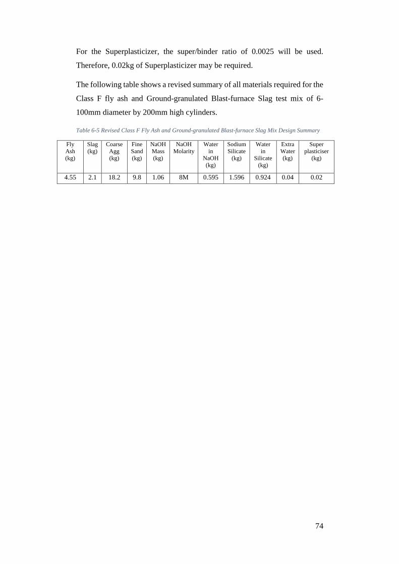
74

For the Superplasticizer, the super/binder ratio of 0.0025 will be used.

Therefore, 0.02kg of Superplasticizer may be required.

The following table shows a revised summary of all materials required for the

Class F fly ash and Ground-granulated Blast-furnace Slag test mix of 6-

100mm diameter by 200mm high cylinders.

Table 6-5 Revised Class F Fly Ash and Ground-granulated Blast-furnace Slag Mix Design Summary

Fly

Ash

(kg)

Slag

(kg)

Coarse

Agg

(kg)

Fine

Sand

(kg)

NaOH

Mass

(kg)

NaOH

Molarity

Water

in

NaOH

(kg)

Sodium

Silicate

(kg)

Water

in

Silicate

(kg)

Extra

Water

(kg)

Super

plasticiser

(kg)

4.55 2.1 18.2 9.8 1.06 8M 0.595 1.596 0.924 0.04 0.02

75

CHAPTER 7 CONCLUSION

It is obvious that global warming has had an effect on the world climate over

the last decade. And with this recognition, we must acknowledge that we have

the power to help rectify the damage that mankind is causing to the planet.

One way of reducing the greenhouse gas emissions is to develop alternate

methods for the production of concrete. Geopolymer Concrete (GPC) is the

method in our salvation. Of course it will not remove the damage already

done but it will help reduce any further harm. If the technology and materials

are available for use today, then it is the responsibility of all within the

construction industry to use these materials. The government should set

targets for greenhouse gas emission reductions and each manufacturer should

be monitored and penalised for exceeding the limits.

It is not enough to say that it may cost a little more per cubic metre or may

take a little longer to reach site. These issues should be taken into account at

the start of the project and included in the cost and scheduling estimates

before construction has begun.

By using the works developed in this project, society is well on the way to

implementing a sustainable replacement for Ordinary Portland Cement

(OPC).

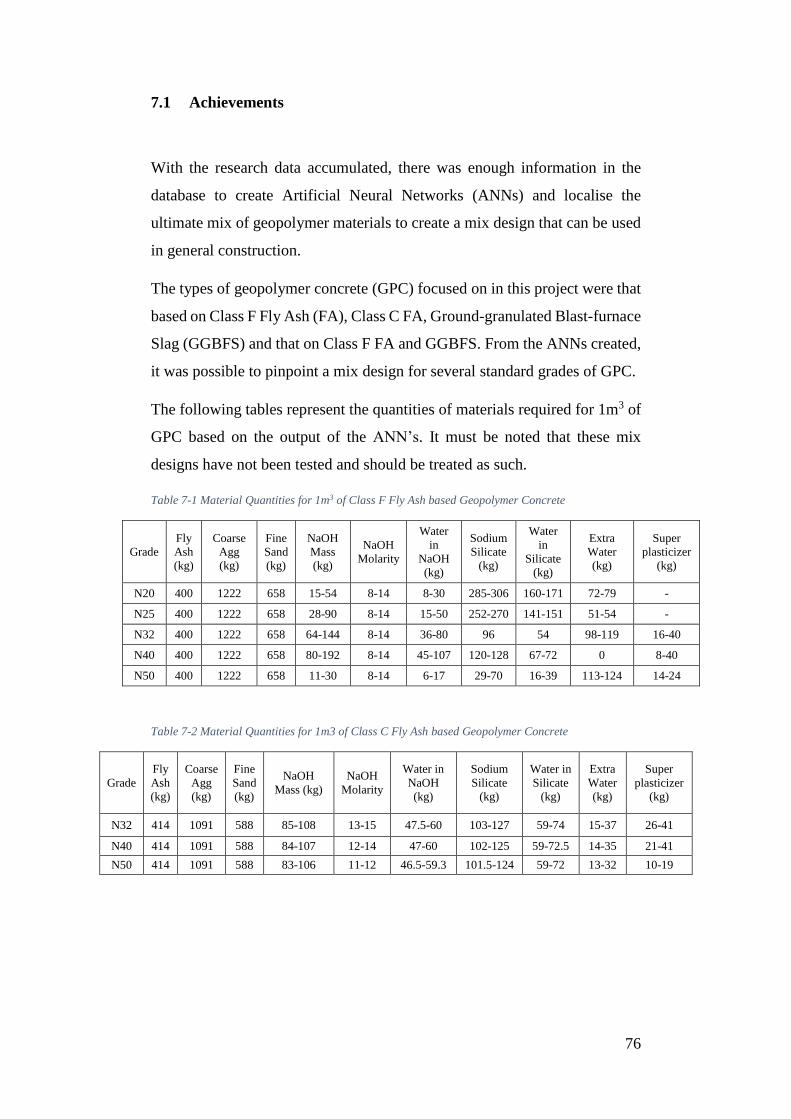
76

7.1 Achievements

With the research data accumulated, there was enough information in the

database to create Artificial Neural Networks (ANNs) and localise the

ultimate mix of geopolymer materials to create a mix design that can be used

in general construction.

The types of geopolymer concrete (GPC) focused on in this project were that

based on Class F Fly Ash (FA), Class C FA, Ground-granulated Blast-furnace

Slag (GGBFS) and that on Class F FA and GGBFS. From the ANNs created,

it was possible to pinpoint a mix design for several standard grades of GPC.

The following tables represent the quantities of materials required for 1m3 of

GPC based on the output of the ANN’s. It must be noted that these mix

designs have not been tested and should be treated as such.

Table 7-1 Material Quantities for 1m3 of Class F Fly Ash based Geopolymer Concrete

Grade

Fly

Ash

(kg)

Coarse

Agg

(kg)

Fine

Sand

(kg)

NaOH

Mass

(kg)

NaOH

Molarity

Water

in

NaOH

(kg)

Sodium

Silicate

(kg)

Water

in

Silicate

(kg)

Extra

Water

(kg)

Super

plasticizer

(kg)

N20 400 1222 658 15-54 8-14 8-30 285-306 160-171 72-79 -

N25 400 1222 658 28-90 8-14 15-50 252-270 141-151 51-54 -

N32 400 1222 658 64-144 8-14 36-80 96 54 98-119 16-40

N40 400 1222 658 80-192 8-14 45-107 120-128 67-72 0 8-40

N50 400 1222 658 11-30 8-14 6-17 29-70 16-39 113-124 14-24

Table 7-2 Material Quantities for 1m3 of Class C Fly Ash based Geopolymer Concrete

Grade

Fly

Ash

(kg)

Coarse

Agg

(kg)

Fine

Sand

(kg)

NaOH

Mass (kg)

NaOH

Molarity

Water in

NaOH

(kg)

Sodium

Silicate

(kg)

Water in

Silicate

(kg)

Extra

Water

(kg)

Super

plasticizer

(kg)

N32 414 1091 588 85-108 13-15 47.5-60 103-127 59-74 15-37 26-41

N40 414 1091 588 84-107 12-14 47-60 102-125 59-72.5 14-35 21-41

N50 414 1091 588 83-106 11-12 46.5-59.3 101.5-124 59-72 13-32 10-19

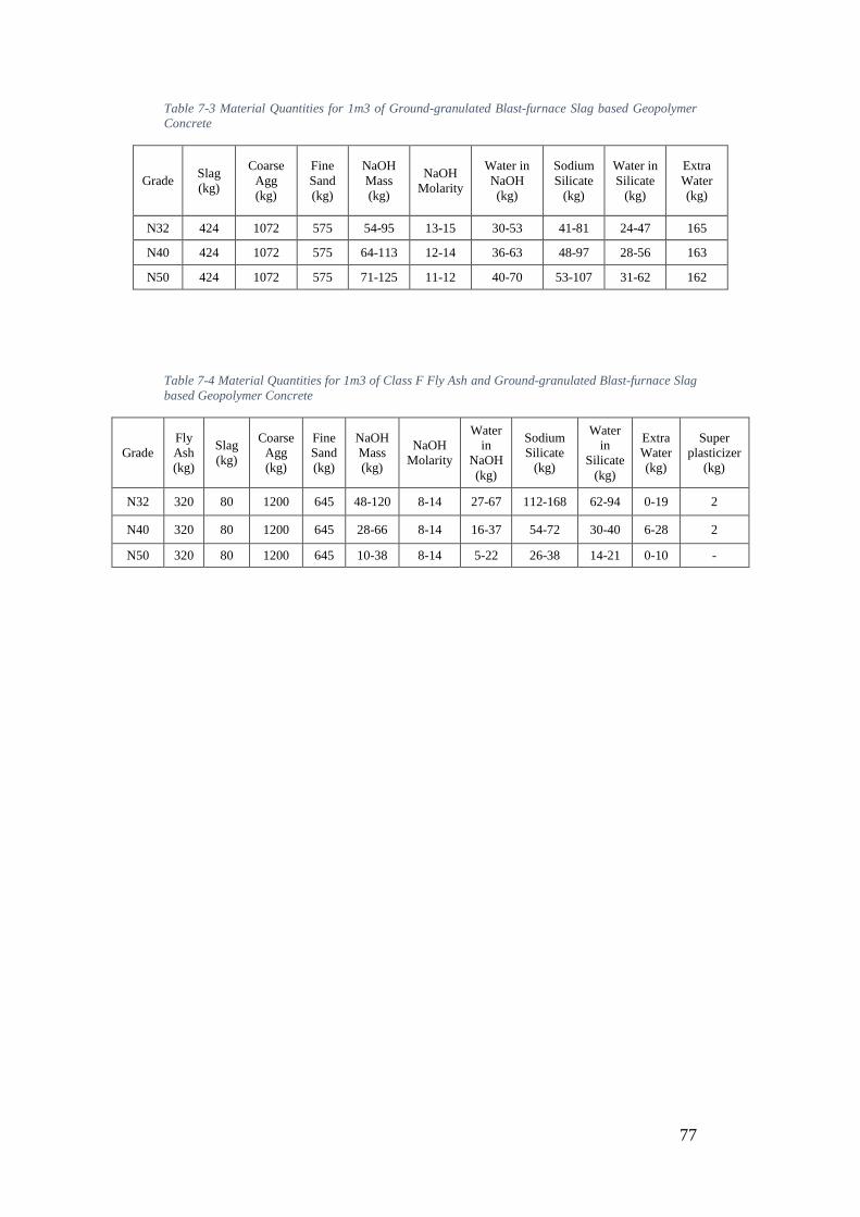
77

Table 7-3 Material Quantities for 1m3 of Ground-granulated Blast-furnace Slag based Geopolymer

Concrete

Grade Slag

(kg)

Coarse

Agg

(kg)

Fine

Sand

(kg)

NaOH

Mass

(kg)

NaOH

Molarity

Water in

NaOH

(kg)

Sodium

Silicate

(kg)

Water in

Silicate

(kg)

Extra

Water

(kg)

N32 424 1072 575 54-95 13-15 30-53 41-81 24-47 165

N40 424 1072 575 64-113 12-14 36-63 48-97 28-56 163

N50 424 1072 575 71-125 11-12 40-70 53-107 31-62 162

Table 7-4 Material Quantities for 1m3 of Class F Fly Ash and Ground-granulated Blast-furnace Slag

based Geopolymer Concrete

Grade

Fly

Ash

(kg)

Slag

(kg)

Coarse

Agg

(kg)

Fine

Sand

(kg)

NaOH

Mass

(kg)

NaOH

Molarity

Water

in

NaOH

(kg)

Sodium

Silicate

(kg)

Water

in

Silicate

(kg)

Extra

Water

(kg)

Super

plasticizer

(kg)

N32 320 80 1200 645 48-120 8-14 27-67 112-168 62-94 0-19 2

N40 320 80 1200 645 28-66 8-14 16-37 54-72 30-40 6-28 2

N50 320 80 1200 645 10-38 8-14 5-22 26-38 14-21 0-10 -

78

7.2 Future work

It is noted that the curing methods from the database were not all consistent

or reflective of ambient conditions, which would be expected in real world

applications. With this acknowledgement, it is advised that more testing be

carried out based around ambient curing temperatures and then repeat the

ANN process to pinpoint an ultimate mix for GPC.

As previously mentioned, the sodium silicate in the database and ANNs was

based on the silicate as a powder and then mixed with water. To fully take

advantage of the ANN results, it is suggested to use sodium silicate powder

instead of pre-made sodium silicate solution. This would also ensure that the

correct water content is used.

It would also be suggested that the revised mix design summary in Table 6-5

be tested first before proceeding onto other mix designs for testing purposes.

To fully cover the range of standard concrete grades, more testing of higher

grades, i.e. 50MPa and above would need to be completed as well as more

testing of slag only mixes and Class C FA mixes. This would overcome the

inconsistencies with the ANN outputs due to lack of training data. It would

then be advised to create ANNs again to determine the ultimate mix for each

type of mixture. The quantities shown in Tables 7-1 to 7-4 would provide an

excellent starting point for testing.

79

References

BARBER, S. 2010. Final Year Project Report. Curtin University.

BERKELMANS, L. W., HAO 2012. Chinese Urban Residential Construction

to 2040. Reserve Bank of Australia.

BERNAL, S. A., MEJÍA DE GUTIÉRREZ, R. & PROVIS, J. L. 2012.

Engineering and durability properties of concretes based on alkali-

activated granulated blast furnace slag/metakaolin blends.

Construction and Building Materials, 33, 99-108.

BONDAR, D. 2011. The Use of Artifical Neural Networks to Predict

Compressive Strength of Geopolymers.

CHI, M. 2012. Effects of dosage of alkali-activated solution and curing

conditions on the properties and durability of alkali-activated slag

concrete. Construction and Building Materials, 35, 240-245.

CHINDAPRASIRT, P., CHAREERAT, T. & SIRIVIVATNANON, V. 2007.

Workability and strength of coarse high calcium fly ash geopolymer.

Cement and Concrete Composites, 29, 224-229.

DAVIDOVITS, J. 1994. Global Warming Impact on the Cement and

Aggregates Industries. World Resource Review, 6, 263-278.

DEB, P. S., NATH, P. & SARKER, P. K. 2014. The effects of ground

granulated blast-furnace slag blending with fly ash and activator

content on the workability and strength properties of geopolymer

concrete cured at ambient temperature. Materials & Design, 62, 32-

39.

DEEVASAN, K. K. & RANGANATH, R. V. 2011. Geopolymer concrete

using industrial byproducts. Proceedings of the Institution of Civil

Engineers, 164, 43-50.

ECONOMIST 2011. Building Rome in a day, The sustainability of China’s

housing boom. The Economist Intelligence Uni.

FERDOUS, W., MANALO, A., KHENNANE, A. & KAYALI, O. 2015.

Geopolymer concrete-filled pultruded composite beams – Concrete

mix design and application. Cement and Concrete Composites, 58, 1-

13.

GALVIN, B. & LLOYD, N. 2011. Fly Ash Based Geopolymer Concrete with

Recycled Concrete Aggregate. Curtin University.

GLASBY, T. 2012. Wagners Earth Friendly Concrete - Global Change

Institute (GCI) Building. Wagners EFC Project Briefing.

HARDJITO, D. 2005. Studies on Fly Ash-Based Geopolymer Concrete.

HARDJITO, D. & RANGAN, B. V. 2005. Development and properties of

Low-Calcium Fly Ash Based Geopolymer Concrete. Curtin

University.

HARDJITO, D., WALLAH, S. E., SUMAJOUW, D. M. & RANGAN, B. V.

2005. Fly Ash-based Geopolymer Concrete. Australian Journal of

Structural Engineering, 6, 77-85.

JOSEPH, B. & MATHEW, G. 2012. Influence of aggregate content on the

behavior of fly ash based geopolymer concrete. Scientia Iranica, 19,

1188-1194.

80

KONG, D. L. Y. & SANJAYAN, J. G. 2010. Effect of elevated temperatures

on geopolymer paste, mortar and concrete. Cement and Concrete

Research, 40, 334-339.

KUSBIANTORO, A., NURUDDIN, M. F., SHAFIQ, N. & QAZI, S. A.

2012. The effect of microwave incinerated rice husk ash on the

compressive and bond strength of fly ash based geopolymer concrete.

Construction and Building Materials, 36, 695-703.

LLOYD, N. A. & RANGAN, B. V. 2010. Geopolymer Concrete with Fly

Ash. Curtin University.

M. FAREED AHMED, M. F. N., AND NASIR SHAFIQ 2011. Compressive

Strength and Workability Characteristics of Low-Calcium Fly ash-

based Self-Compacting Geopolymer Concrete. World Academy of

Science, Engineering and Technology, 74, 8-14.

MEMON, F. A., NURUDDIN, M. F., DEMIE, S. & SHAFIQ, N. 2011. Effect

of Curing Conditions on Strength of Fly ash-based Self-Compacting

Geopolymer Concrete. World Academy of Science, Engineering and

Technology, 80, 860-863.

NATH, P. & SARKER, P. K. 2014. Effect of GGBFS on setting, workability

and early strength properties of fly ash geopolymer concrete cured in

ambient condition. Construction and Building Materials, 66, 163-171.

NAZARI, A. & TORGAL, F. P. 2012. Predicting compressive strength of

different geopolymer by artificial neural networks. Ceramics

International, 39, 2247-2257.

OLIVIA, M. & NIKRAZ, H. 2011. Properties of fly ash geopolymer concrete

designed by Taguchi method. Materials and Design, 36 191–198.

RADLINSKI, M. H., N ; MONCARZ,P 2011. Sustainable Concrete: Impacts

of Existing and Emerging Materials and Technologies on the

Construction Industry.

RAHMAN, M. M. & SARKER, P. K. 2011. Geopolymer Concrete Columns

under Combined Axial Load and Biaxial Bending. Curtin University.

RANGAN, S. E. W. A. B. V. 2006. LOW-CALCIUM FLY ASH-BASED

GEOPOLYMER CONCRETE: LONG-TERM PROPERTIES.

SARKER, P. K., HAQUE, R. & RAMGOLAM, K. V. 2013. Fracture

behaviour of heat cured fly ash based geopolymer concrete. Materials

& Design, 44, 580-586.

SHI, X. S., COLLINS, F. G., ZHAO, X. L. & WANG, Q. Y. 2012.

Mechanical properties and microstructure analysis of fly ash

geopolymeric recycled concrete. Journal of Hazardous Materials,

237–238, 20-29.

SHOJAEI, M., BEHFARNIA, K. & MOHEBI, R. 2015. Application of

alkali-activated slag concrete in railway sleepers. Materials & Design,

69, 89-95.

SUMAJOUW, M. D. J. & RANGAN, B. V. 2006. LOW-CALCIUM FLY

ASH-BASED GEOPOLYMER CONCRETE: REINFORCED

BEAMS AND COLUMNS.

T. SUJATHA, K. K. A. S. N. 2012. STRENGTH ASSESSMENT OF HEAT

CURED GEOPOLYMER CONCRETE SLENDER COLUMN.

ASIAN JOURNALOF CIVIL ENGINEERING (BUILDING

ANDHOUSING)

VOL. 13, PAGES 635-646.

81

TALHA JUNAID, M., KAYALI, O., KHENNANE, A. & BLACK, J. 2015.

A mix design procedure for low calcium alkali activated fly ash-based

concretes. Construction and Building Materials, 79, 301-310.

THOMAS, M. 2007. Optimizing the Use of Fly Ash in Concrete.

TOPARK-NGARM, P., CHINDAPRASIRT, P. & SATA, V. 2014. Setting

Time, Strength, and Bond of High-Calcium Fly Ash Geopolymer

Concrete.

TOPÇU, İ. B., KARAKURT, C. & SARıDEMIR, M. 2008. Predicting the

strength development of cements produced with different pozzolans

by neural network and fuzzy logic. Materials & Design, 29, 1986-

1991.

TOPÇU, İ. B. & SARıDEMIR, M. 2008. Prediction of compressive strength

of concrete containing fly ash using artificial neural networks and

fuzzy logic. Computational Materials Science, 41, 305-311.

TURNER, L. K. & COLLINS, F. G. 2013. Carbon dioxide equivalent (CO2-

e) emissions: A comparison between geopolymer and OPC cement

concrete. Construction and Building Materials, 43, 125-130.

VORA, P. R. & DAVE, U. V. 2013. Parametric Studies on Compressive

Strength of Geopolymer Concrete. Procedia Engineering, 51, 210-

219.

XIE, T. & OZBAKKALOGLU, T. 2015. Behavior of low-calcium fly and

bottom ash-based geopolymer concrete cured at ambient temperature.

Ceramics International, 41, 5945-5958.

SUHENDRO, B. (2014). Toward Green Concrete for Better Sustainable

Environment. Procedia Engineering, 95: 305-320.

CCANZ (1989). The Manufacture of Portland Cement, The Cement and

Concrete Association of New Zealand.

FLY ASH AUSTRALIA (2010). “What is Fly Ash”,

www.flyashaustralia.com.au/WhatIsFlyash.aspx

CEMENT AUSTRALIA (2014). “Slag”,

http://www.cementaustralia.com.au/wps/wcm/connect/website/bulk/Bulk-

Home/our-products/slag/

QUEENSLAND GOVERNMENT (2012). “Safe Use of Laptops”,

Organisational Health, Department of Education, Training and

Employment.

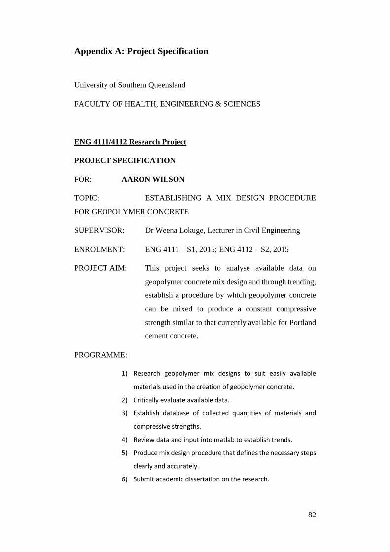
82

Appendix A: Project Specification

University of Southern Queensland

FACULTY OF HEALTH, ENGINEERING & SCIENCES

ENG 4111/4112 Research Project

PROJECT SPECIFICATION

FOR: AARON WILSON

TOPIC: ESTABLISHING A MIX DESIGN PROCEDURE

FOR GEOPOLYMER CONCRETE

SUPERVISOR: Dr Weena Lokuge, Lecturer in Civil Engineering

ENROLMENT: ENG 4111 – S1, 2015; ENG 4112 – S2, 2015

PROJECT AIM: This project seeks to analyse available data on

geopolymer concrete mix design and through trending,

establish a procedure by which geopolymer concrete

can be mixed to produce a constant compressive

strength similar to that currently available for Portland

cement concrete.

PROGRAMME:

1) Research geopolymer mix designs to suit easily available

materials used in the creation of geopolymer concrete.

2) Critically evaluate available data.

3) Establish database of collected quantities of materials and

compressive strengths.

4) Review data and input into matlab to establish trends.

5) Produce mix design procedure that defines the necessary steps

clearly and accurately.

6) Submit academic dissertation on the research.

83

As time permits:

7) Choose 2 mix designs relating to 32MPa concrete for testing.

8) Gather materials and mix concrete for testing.

9) Test samples and compare results to the gathered data.

AGREED Student: Aaron Wilson Date: 31/03/15

Supervisor: Weena Lokuge Date: 31/03/15

Examiner: Chris Snook

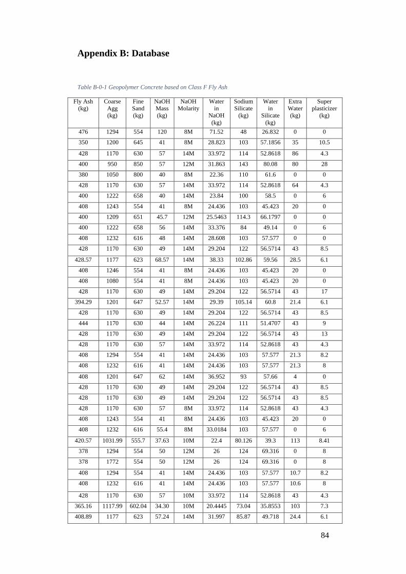
84

Appendix B: Database

Table B-0-1 Geopolymer Concrete based on Class F Fly Ash

Fly Ash

(kg)

Coarse

Agg

(kg)

Fine

Sand

(kg)

NaOH

Mass

(kg)

NaOH

Molarity

Water

in

NaOH

(kg)

Sodium

Silicate

(kg)

Water

in

Silicate

(kg)

Extra

Water

(kg)

Super

plasticizer

(kg)

476 1294 554 120 8M 71.52 48 26.832 0 0

350 1200 645 41 8M 28.823 103 57.1856 35 10.5

428 1170 630 57 14M 33.972 114 52.8618 86 4.3

400 950 850 57 12M 31.863 143 80.08 80 28

380 1050 800 40 8M 22.36 110 61.6 0 0

428 1170 630 57 14M 33.972 114 52.8618 64 4.3

400 1222 658 40 14M 23.84 100 58.5 0 6

408 1243 554 41 8M 24.436 103 45.423 20 0

400 1209 651 45.7 12M 25.5463 114.3 66.1797 0 0

400 1222 658 56 14M 33.376 84 49.14 0 6

408 1232 616 48 14M 28.608 103 57.577 0 0

428 1170 630 49 14M 29.204 122 56.5714 43 8.5

428.57 1177 623 68.57 14M 38.33 102.86 59.56 28.5 6.1

408 1246 554 41 8M 24.436 103 45.423 20 0

408 1080 554 41 8M 24.436 103 45.423 20 0

428 1170 630 49 14M 29.204 122 56.5714 43 17

394.29 1201 647 52.57 14M 29.39 105.14 60.8 21.4 6.1

428 1170 630 49 14M 29.204 122 56.5714 43 8.5

444 1170 630 44 14M 26.224 111 51.4707 43 9

428 1170 630 49 14M 29.204 122 56.5714 43 13

428 1170 630 57 14M 33.972 114 52.8618 43 4.3

408 1294 554 41 14M 24.436 103 57.577 21.3 8.2

408 1232 616 41 14M 24.436 103 57.577 21.3 8

408 1201 647 62 14M 36.952 93 57.66 4 0

428 1170 630 49 14M 29.204 122 56.5714 43 8.5

428 1170 630 49 14M 29.204 122 56.5714 43 8.5

428 1170 630 57 8M 33.972 114 52.8618 43 4.3

408 1243 554 41 8M 24.436 103 45.423 20 0

408 1232 616 55.4 8M 33.0184 103 57.577 0 6

420.57 1031.99 555.7 37.63 10M 22.4 80.126 39.3 113 8.41

378 1294 554 50 12M 26 124 69.316 0 8

378 1772 554 50 12M 26 124 69.316 0 8

408 1294 554 41 14M 24.436 103 57.577 10.7 8.2

408 1232 616 41 14M 24.436 103 57.577 10.6 8

428 1170 630 57 10M 33.972 114 52.8618 43 4.3

365.16 1117.99 602.04 34.30 10M 20.4445 73.04 35.8553 103 7.3

408.89 1177 623 57.24 14M 31.997 85.87 49.718 24.4 6.1

85

408 1294 554 51.5 14M 30.694 103 57.577 16.5 16.3

408 1294 554 41 14M 22.919 103 61.388 22.5 6

408 1201 647 62 14M 36.952 93 57.66 0 0

428 1170 630 49 14M 29.204 122 56.5714 43 8.5

408 1294 554 41 14M 24.436 103 57.577 22.5 6

254.54 1290 694.66 22.77 10M 13.5709 48.49 23.8037 68.7 5.1

408 1201 647 41 14M 24.436 103 57.577 20.7 6.1

406 1194 643 41 14M 24.436 102 57.018 26.8 6

404 1190 640 41 14M 24.436 102 57.018 25.5 6

480 1153 599 56 14M 31.304 112 64.848 23.7 6.1

400 950 850 57 12M 31.863 143 80.08 60 28

408 1201 647 41 12M 24.436 103 57.577 14.3 6.1

428 1170 630 57 14M 33.972 114 52.8618 43 4.3

444.44 1177 623 44.44 14M 24.8419 111.11 64.3327 18.6 6.1

498.46 1153 599 59.82 14M 33.439 89.72 51.9478 26.5 6.1

408 1201 647 41 12M 24.436 103 57.577 14.3 6.1

408 1201 647 41 14M 24.436 103 57.577 20.7 6.1

408 1201 647 41 16M 24.436 103 57.577 26.5 6.1

408 1294 554 41 14M 24.436 103 57.577 16.5 6.1

428 1170 630 57 14M 33.972 114 52.8618 43 8.5

408 1294 554 51.5 14M 30.694 103 57.577 16.5 4.1

408 1294 554 51.5 14M 30.694 103 57.577 16.5 8.2

408 1232 616 55.4 8M 33.0184 103 57.577 0 6

408 1294 554 51.5 14M 30.694 103 57.577 16.5 0

408 1201 647 41 12M 24.436 103 57.577 14.4 6.1

309.85 1204 648.35 27.73 10M 16.5270 59.03 28.97 83.6 6.2

408 1202 647 41 16M 24.436 103 57.577 26 6

461.54 1177 623 46.15 14M 25.7978 92.31 53.44 18.6 6.1

408 1201 647 41 14M 24.436 103 57.577 17.6 6.1

428 1170 630 57 12M 33.972 114 52.8618 43 4.3

408 1294 554 41 14M 24.436 103 57.577 0 8.2

408 1201 647 55.4 8M 33.0184 103 57.577 0 6.1

400 1265 540 42.3 16M 25.2108 105.7 59.086 24.3 4.2

400 950 850 57 12M 31.863 143 80.08 48 28

408 1201 647 41 10M 24.436 103 57.577 7.5 6.1

408 1232 616 41 14M 24.436 103 57.577 20.7 6

408 1232 616 41 14M 24.436 103 57.577 0 8

408 1294 554 41 14M 27.88 103 57.577 22.5 6

428 1170 630 49 14M 29.204 122 56.5714 43 8.5

408 1294 554 41 14M 24.436 103 57.577 22.5 6

400 950 850 57 12M 31.863 143 80.08 48 28

405 1235 545 52.9 16M 31.53 132.4 74.012 28 3

404 1190 640 41 14M 24.436 102 57.018 17 6

428 1170 630 57 14M 33.972 114 52.8618 43 4.3

86

428 1170 630 57 14M 33.972 114 52.8618 43 4.3

408 1201 647 41 8M 24.436 103 57.577 0 6.1

400 950 850 57 12M 31.863 143 80.08 48 28

476 1294 554 120 14M 71.52 48 26.832 0 0

408 1232 616 41 16M 24.436 103 57.577 26.5 6

350 1200 645 41 8M 28.823 103 57.1856 35 0

408 1201 647 68 14M 40.528 103 63.86 0 0

400 950 850 57 12M 31.863 144 81.0864 48 28

400 950 850 57 12M 31.863 143 80.08 48 28

380 1233 540 56.5 16M 33.674 141.3 78.99 14.6 4

428 1170 630 57 14M 33.972 114 52.8618 43 4.3

462.86 1153 599 52.9 14M 29.5711 132.24 76.56 21.2 6.1

404 1195 640 41 16M 24.436 102 57.018 20 6

408 1232 616 41 12M 24.436 103 57.577 14.4 6

408 1232 616 41 8M 24.436 103 57.577 0 6

400 950 850 57 12M 31.863 143 80.08 48 28

400 950 850 57 12M 31.863 143 80.08 48 28

400 950 850 57 12M 31.863 143 80.08 48 28

408 1232 616 41 10M 24.436 103 57.577 7.5 6

400 1356 535 51.5 16M 30.694 128.6 71.89 12.7 4.2

400 950 850 57 12M 31.863 143 80.08 40 28

408 1201 647 63 12M 32.76 138 77.142 0 8

408 723 647 63 12M 32.76 138 77.142 0 8

368 1294 554 53 8M 31.588 131 73.229 0 0

424.62 1177 623 36.4 14M 20.3476 90.99 52.68 15.9 6.1

408 1201 647 55.4 8M 33.0184 103 57.577 0 6.1

408 1232 616 41 8M 24.436 103 57.577 0 6

408 1294 554 41 8M 22.919 103 61.388 0 6

408 1294 554 41 8M 24.436 103 57.577 0 6

532.8 0 1600.8 41 8M 22.919 102.5 57.2975 0 0

476 1294 554 48 8M 28.608 120 67.08 0 0

408 1294 554 41 8M 27.88 103 57.577 0 6

408 1294 554 41 8M 24.436 103 57.577 0 6

408 1232 616 48 8M 28.608 103 57.577 0 0

408 1201 647 41 8M 24.436 103 57.577 0 6.1

404 1190 640 41 14M 24.436 102 57.018 16.5 6

408 1232 616 41 14M 24.436 103 57.577 0 8

476 1294 554 48 14M 28.608 120 67.08 0 0

408 1201 647 41 8M 24.436 103 57.577 0 6.1

420 1125 750 40 22.36 100 55.9 0 0

368 1294 554 53 8M 31.588 131 73.229 0 0

404 1190 640 41 14M 24.436 102 57.018 13.5 6

368 1294 554 53 8M 31.588 131 73.229 0 0

408 1201 647 41 14M 24.436 103 57.577 0 8.2

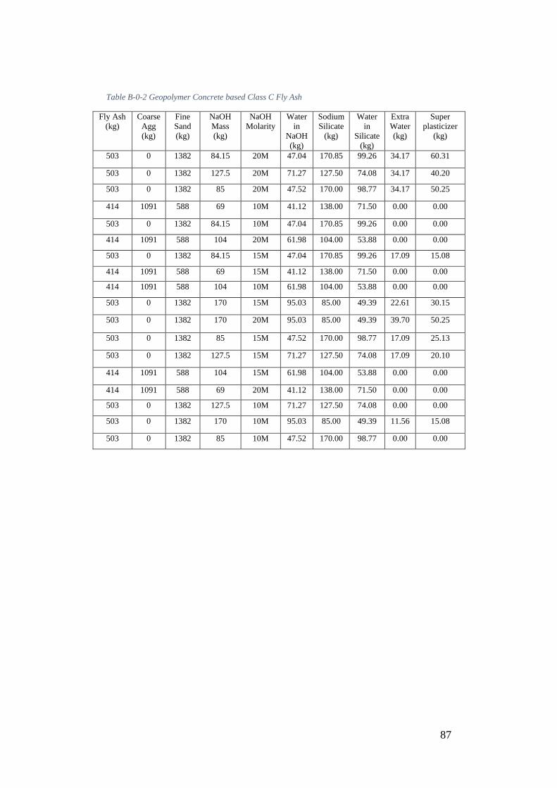
87

Table B-0-2 Geopolymer Concrete based Class C Fly Ash

Fly Ash

(kg)

Coarse

Agg

(kg)

Fine

Sand

(kg)

NaOH

Mass

(kg)

NaOH

Molarity

Water

in

NaOH

(kg)

Sodium

Silicate

(kg)

Water

in

Silicate

(kg)

Extra

Water

(kg)

Super

plasticizer

(kg)

503 0 1382 84.15 20M 47.04 170.85 99.26 34.17 60.31

503 0 1382 127.5 20M 71.27 127.50 74.08 34.17 40.20

503 0 1382 85 20M 47.52 170.00 98.77 34.17 50.25

414 1091 588 69 10M 41.12 138.00 71.50 0.00 0.00

503 0 1382 84.15 10M 47.04 170.85 99.26 0.00 0.00

414 1091 588 104 20M 61.98 104.00 53.88 0.00 0.00

503 0 1382 84.15 15M 47.04 170.85 99.26 17.09 15.08

414 1091 588 69 15M 41.12 138.00 71.50 0.00 0.00

414 1091 588 104 10M 61.98 104.00 53.88 0.00 0.00

503 0 1382 170 15M 95.03 85.00 49.39 22.61 30.15

503 0 1382 170 20M 95.03 85.00 49.39 39.70 50.25

503 0 1382 85 15M 47.52 170.00 98.77 17.09 25.13

503 0 1382 127.5 15M 71.27 127.50 74.08 17.09 20.10

414 1091 588 104 15M 61.98 104.00 53.88 0.00 0.00

414 1091 588 69 20M 41.12 138.00 71.50 0.00 0.00

503 0 1382 127.5 10M 71.27 127.50 74.08 0.00 0.00

503 0 1382 170 10M 95.03 85.00 49.39 11.56 15.08

503 0 1382 85 10M 47.52 170.00 98.77 0.00 0.00

88

Table B-0-3 Geopolymer Concrete based on Ground-granulated Blast-furnace Slag

Slag

(kg)

Coarse

Agg

(kg)

Fine

Sand

(kg)

NaOH

Mass

(kg)

NaOH

Molarity

Water

in

NaOH

(kg)

Sodium

Silicate

(kg)

Water

in

Silicate

(kg)

Extra

Water

(kg)

Super

plasticizer

(kg)

400 860 860 84 8M 46.96 28.00 15.68 156.0 0

400 844 844 76 8M 42.48 76.00 42.56 144.0 0

394.3 1232 616 131.4 73.45 26.30 12.10 67.60 0

424 1072 575 13 8M 7.27 46.50 26.04 216.0 0

424 1072 575 16.3 8M 9.11 58.10 32.54 212.0 0

424 1072 575 19.5 8M 10.90 69.70 39.03 208.0 0

380.7 1232 616 128.5 71.83 42.80 19.69 41.20 0

360 1264 632 108 60.37 36.00 16.56 58.80 0

336 1264 632 140 78.26 28.00 12.88 17.60 0

368 1232 616 92 51.43 92.00 42.32 58.80 0

428.6 1200 600 85.7 47.91 85.70 39.42 83.30 0

413.8 1200 600 155.2 86.76 31.00 14.26 47.00 0

400 1200 600 150 83.85 50.00 23.00 52.90 0

400 832 832 68 8M 38.01 120.00 67.20 132.0 0

347.6 1264 632 78.2 43.71 78.20 35.97 70.60 0

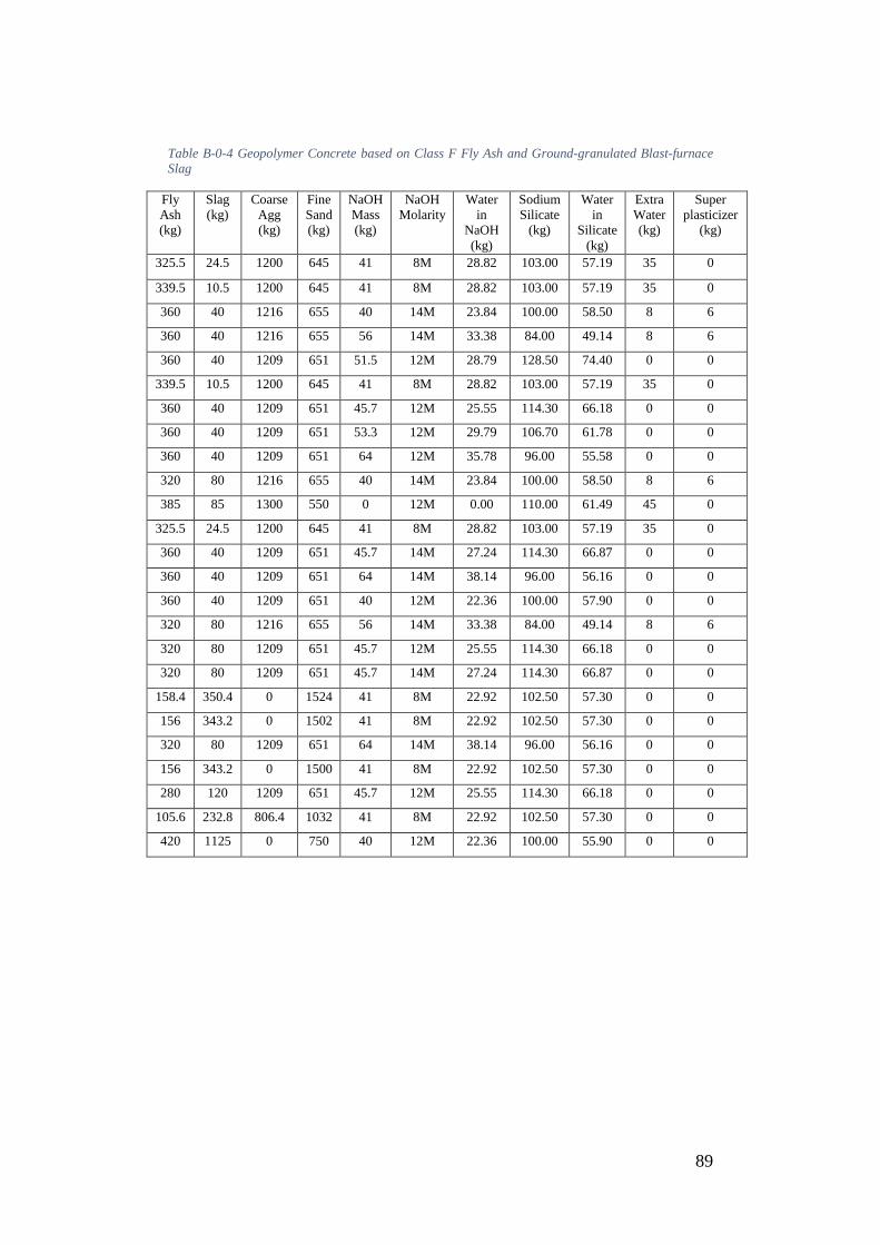
89

Table B-0-4 Geopolymer Concrete based on Class F Fly Ash and Ground-granulated Blast-furnace

Slag

Fly

Ash

(kg)

Slag

(kg)

Coarse

Agg

(kg)

Fine

Sand

(kg)

NaOH

Mass

(kg)

NaOH

Molarity

Water

in

NaOH

(kg)

Sodium

Silicate

(kg)

Water

in

Silicate

(kg)

Extra

Water

(kg)

Super

plasticizer

(kg)

325.5 24.5 1200 645 41 8M 28.82 103.00 57.19 35 0

339.5 10.5 1200 645 41 8M 28.82 103.00 57.19 35 0

360 40 1216 655 40 14M 23.84 100.00 58.50 8 6

360 40 1216 655 56 14M 33.38 84.00 49.14 8 6

360 40 1209 651 51.5 12M 28.79 128.50 74.40 0 0

339.5 10.5 1200 645 41 8M 28.82 103.00 57.19 35 0

360 40 1209 651 45.7 12M 25.55 114.30 66.18 0 0

360 40 1209 651 53.3 12M 29.79 106.70 61.78 0 0

360 40 1209 651 64 12M 35.78 96.00 55.58 0 0

320 80 1216 655 40 14M 23.84 100.00 58.50 8 6

385 85 1300 550 0 12M 0.00 110.00 61.49 45 0

325.5 24.5 1200 645 41 8M 28.82 103.00 57.19 35 0

360 40 1209 651 45.7 14M 27.24 114.30 66.87 0 0

360 40 1209 651 64 14M 38.14 96.00 56.16 0 0

360 40 1209 651 40 12M 22.36 100.00 57.90 0 0

320 80 1216 655 56 14M 33.38 84.00 49.14 8 6

320 80 1209 651 45.7 12M 25.55 114.30 66.18 0 0

320 80 1209 651 45.7 14M 27.24 114.30 66.87 0 0

158.4 350.4 0 1524 41 8M 22.92 102.50 57.30 0 0

156 343.2 0 1502 41 8M 22.92 102.50 57.30 0 0

320 80 1209 651 64 14M 38.14 96.00 56.16 0 0

156 343.2 0 1500 41 8M 22.92 102.50 57.30 0 0

280 120 1209 651 45.7 12M 25.55 114.30 66.18 0 0

105.6 232.8 806.4 1032 41 8M 22.92 102.50 57.30 0 0

420 1125 0 750 40 12M 22.36 100.00 55.90 0 0

90

Appendix C: Artificial Neural Network Data

Table C-0-1 Class F Fly Ash Artificial Neural Network inputs, targets and predicted outputs

NaOH/

Sodium

Silicate

AL/FA W/GPS Super/Binder NaOH

Molarity

Compressive

Strength

(MPa)

Predicted

Compressive

Strength

0.40 0.41 0.297 0.030 8 20 37.48716327

0.50 0.40 0.337 0.010 14 20 32.35372186

0.40 0.50 0.393 0.070 12 22.58 38.96193747

0.36 0.39 0.188 0.000 8 24 47.78985368

0.50 0.40 0.295 0.010 14 24 34.59840653

0.40 0.35 0.180 0.015 14 25 39.36794657

0.40 0.35 0.186 0.000 8 25 43.38942883

0.40 0.40 0.196 0.000 12 26 37.12317855

0.67 0.35 0.180 0.015 14 27 37.19333897

0.47 0.37 0.182 0.000 14 28 41.77777243

0.40 0.40 0.251 0.020 14 28 36.92748634

0.67 0.40 0.252 0.014 14 28.64 37.29445203

0.40 0.35 0.186 0.000 8 29 43.38942883

0.40 0.35 0.186 0.000 8 29 43.38942883

0.40 0.40 0.251 0.040 14 29 37.0594377

0.50 0.40 0.242 0.015 14 29.71 37.92312669

0.40 0.40 0.251 0.020 14 30 36.92748634

0.40 0.35 0.232 0.020 14 30 37.80030647

0.40 0.40 0.251 0.030 14 30 36.89654396

0.50 0.40 0.253 0.010 14 30 37.32609112

0.40 0.35 0.220 0.020 14 32 38.19369819

0.40 0.35 0.220 0.020 14 32 38.19369819

0.67 0.38 0.211 0.000 14 32 39.75294803

0.40 0.40 0.251 0.020 14 32 36.92748634

0.40 0.40 0.251 0.020 14 32 36.92748634

0.50 0.40 0.253 0.010 8 32 35.15739869

0.40 0.35 0.186 0.000 8 33 43.38942883

0.54 0.39 0.190 0.015 8 33 46.7163224

0.47 0.28 0.368 0.020 10 33.75 47.64114071

0.40 0.46 0.209 0.021 12 34.59 35.63436209

0.40 0.46 0.209 0.021 12 34.6 35.63436209

0.40 0.35 0.197 0.020 14 35 38.96583658

0.40 0.35 0.197 0.020 14 35 38.96583658

0.50 0.40 0.253 0.010 10 35 31.35315684

0.47 0.29 0.384 0.020 10 35.25 46.63194798

0.67 0.35 0.226 0.015 14 35.73 36.40944601

0.50 0.38 0.221 0.040 14 36 39.54479158

0.40 0.35 0.228 0.015 14 36 37.47689344

0.67 0.38 0.202 0.000 14 36 40.40615961

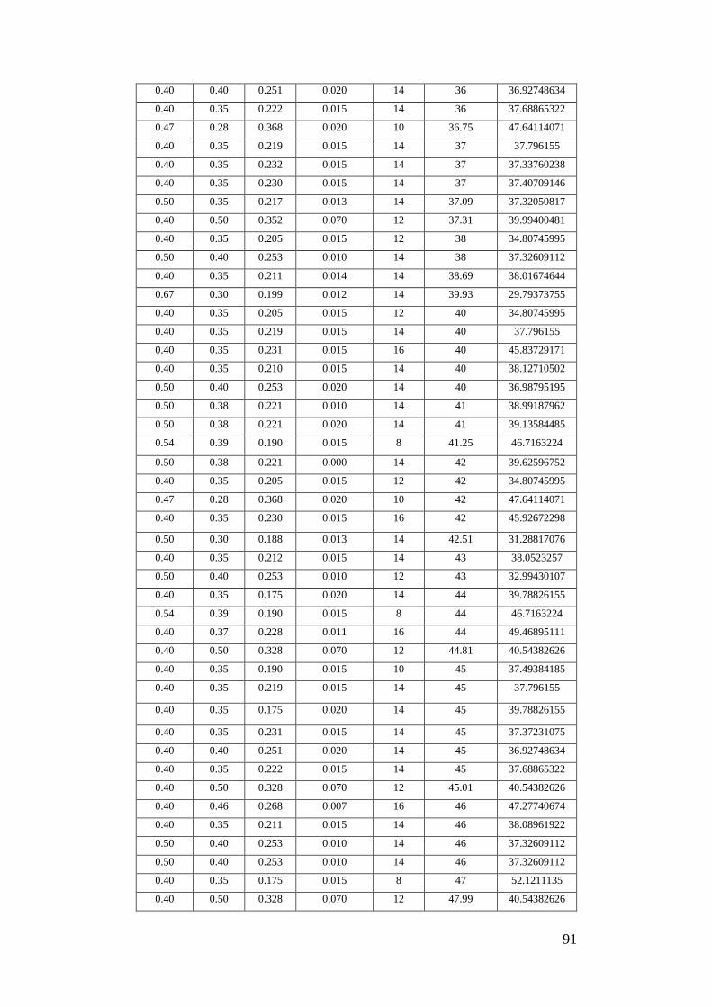
91

0.40 0.40 0.251 0.020 14 36 36.92748634

0.40 0.35 0.222 0.015 14 36 37.68865322

0.47 0.28 0.368 0.020 10 36.75 47.64114071

0.40 0.35 0.219 0.015 14 37 37.796155

0.40 0.35 0.232 0.015 14 37 37.33760238

0.40 0.35 0.230 0.015 14 37 37.40709146

0.50 0.35 0.217 0.013 14 37.09 37.32050817

0.40 0.50 0.352 0.070 12 37.31 39.99400481

0.40 0.35 0.205 0.015 12 38 34.80745995

0.50 0.40 0.253 0.010 14 38 37.32609112

0.40 0.35 0.211 0.014 14 38.69 38.01674644

0.67 0.30 0.199 0.012 14 39.93 29.79373755

0.40 0.35 0.205 0.015 12 40 34.80745995

0.40 0.35 0.219 0.015 14 40 37.796155

0.40 0.35 0.231 0.015 16 40 45.83729171

0.40 0.35 0.210 0.015 14 40 38.12710502

0.50 0.40 0.253 0.020 14 40 36.98795195

0.50 0.38 0.221 0.010 14 41 38.99187962

0.50 0.38 0.221 0.020 14 41 39.13584485

0.54 0.39 0.190 0.015 8 41.25 46.7163224

0.50 0.38 0.221 0.000 14 42 39.62596752

0.40 0.35 0.205 0.015 12 42 34.80745995

0.47 0.28 0.368 0.020 10 42 47.64114071

0.40 0.35 0.230 0.015 16 42 45.92672298

0.50 0.30 0.188 0.013 14 42.51 31.28817076

0.40 0.35 0.212 0.015 14 43 38.0523257

0.50 0.40 0.253 0.010 12 43 32.99430107

0.40 0.35 0.175 0.020 14 44 39.78826155

0.54 0.39 0.190 0.015 8 44 46.7163224

0.40 0.37 0.228 0.011 16 44 49.46895111

0.40 0.50 0.328 0.070 12 44.81 40.54382626

0.40 0.35 0.190 0.015 10 45 37.49384185

0.40 0.35 0.219 0.015 14 45 37.796155

0.40 0.35 0.175 0.020 14 45 39.78826155

0.40 0.35 0.231 0.015 14 45 37.37231075

0.40 0.40 0.251 0.020 14 45 36.92748634

0.40 0.35 0.222 0.015 14 45 37.68865322

0.40 0.50 0.328 0.070 12 45.01 40.54382626

0.40 0.46 0.268 0.007 16 46 47.27740674

0.40 0.35 0.211 0.015 14 46 38.08961922

0.50 0.40 0.253 0.010 14 46 37.32609112

0.50 0.40 0.253 0.010 14 46 37.32609112

0.40 0.35 0.175 0.015 8 47 52.1211135

0.40 0.50 0.328 0.070 12 47.99 40.54382626

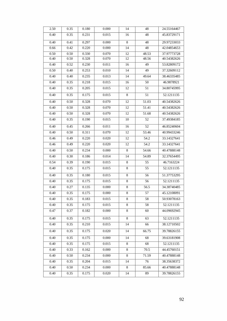
92

2.50 0.35 0.180 0.000 14 48 24.55164467

0.40 0.35 0.231 0.015 16 48 45.83729171

0.40 0.41 0.297 0.000 8 48 29.97233033

0.66 0.42 0.220 0.000 14 48 42.04854653

0.50 0.50 0.330 0.070 12 48.53 37.97773728

0.40 0.50 0.328 0.070 12 48.56 40.54382626

0.40 0.52 0.230 0.011 16 49 53.82809172

0.50 0.40 0.253 0.010 14 49 37.32609112

0.40 0.40 0.235 0.013 14 49.64 38.46335485

0.40 0.35 0.218 0.015 16 50 46.9878921

0.40 0.35 0.205 0.015 12 51 34.80745995

0.40 0.35 0.175 0.015 8 51 52.1211135

0.40 0.50 0.328 0.070 12 51.03 40.54382626

0.40 0.50 0.328 0.070 12 51.41 40.54382626

0.40 0.50 0.328 0.070 12 51.68 40.54382626

0.40 0.35 0.190 0.015 10 52 37.49384185

0.40 0.45 0.266 0.011 16 52 46.85240604

0.40 0.50 0.311 0.070 12 53.46 40.99433246

0.46 0.49 0.220 0.020 12 54.2 33.14327641

0.46 0.49 0.220 0.020 12 54.2 33.14327641

0.40 0.50 0.234 0.000 8 54.66 40.47888148

0.40 0.30 0.186 0.014 14 54.89 32.37654495

0.54 0.39 0.190 0.015 8 55 46.7163224

0.40 0.35 0.175 0.015 8 55 52.1211135

0.40 0.35 0.180 0.015 8 56 51.37753295

0.40 0.35 0.175 0.015 8 56 52.1211135

0.40 0.27 0.135 0.000 8 56.5 34.38740485

0.40 0.35 0.175 0.000 8 57 45.12108091

0.40 0.35 0.183 0.015 8 58 50.93078163

0.40 0.35 0.175 0.015 8 58 52.1211135

0.47 0.37 0.182 0.000 8 60 44.09692945

0.40 0.35 0.175 0.015 8 63 52.1211135

0.40 0.35 0.210 0.015 14 66 38.12710502

0.40 0.35 0.175 0.020 14 66.75 39.78826155

0.40 0.35 0.175 0.000 14 68 39.63181908

0.40 0.35 0.175 0.015 8 68 52.1211135

0.40 0.33 0.162 0.000 8 70.5 44.45760151

0.40 0.50 0.234 0.000 8 71.59 40.47888148

0.40 0.35 0.204 0.015 14 76 38.35638372

0.40 0.50 0.234 0.000 8 85.66 40.47888148

0.40 0.35 0.175 0.020 14 89 39.78826155

93

Appendix D: Sample Matlab Plotfile

% Aaron Wilson Student Number 0050052015 %GGBFS Plot File.

%inputs %NaOH/Sodium Silicate Ratio NaS = slag_inputs(:,4)'; NaSnodes = 0.1:0.01:1;

%AL/Slag Ratio ALslag = slag_inputs(:,5)'; ALslagnodes = 0:0.01:0.55;

%Water/Geopolymer Solids Ratio WGPS = slag_inputs(:,6)'; WGPSnodes = 0.4:0.01:0.55;

%Outputs z = ANN_slag_outputs';

%% %Al/Slag Vs W/GPS

%fit data to surface Z = gridfit(ALslag,WGPS,z,ALslagnodes,WGPSnodes);

%plot the file

figure [A,b]= contourf(ALslagnodes,WGPSnodes,Z); clabel(A,b) title ('Ground Granulated Blast Furnace Slag - AL/Slag Vs

Water/Geopolymer Solids') xlabel ('AL/Slag') ylabel ('W/GPS') print('slag - AL_Slag Vs W_GPS', '-djpeg', '-r300') %% %NaOh/Sodium Silicate Vs Al/Slag

%fit data to surface Z2 = gridfit(NaS,ALslag,z,NaSnodes,ALslagnodes);

%plot the file

figure [B,c]= contourf(NaSnodes,ALslagnodes,Z2); clabel(B,c) title ('Ground Granulated Blast Furnace Slag - NaOH/Sodium

Silicate Vs AL/Slag') xlabel ('NaOH/Sodium Silicate') ylabel ('AL/Slag') print('slag - NaOH_Silic Vs AL_Slag', '-djpeg', '-r300') %% %NaOh/Sodium Silicate Vs W/GPS

94

Z3 = gridfit(NaS,WGPS,z,NaSnodes,WGPSnodes);

%plot the file

figure [C,d]= contourf(NaSnodes,WGPSnodes,Z3); clabel(C,d) title ('Ground Granulated Blast Furnace Slag - NaOH/Sodium

Silicate Vs Water/Geopolymer Solids') xlabel ('NaOH/Sodium Silicate') ylabel ('W/GPS') print('slag - NaOH_Silic Vs W_GPS', '-djpeg', '-r300')

establishing a mix design procedure for … of southern queensland faculty of health, engineering...

Documents