establishing metrics for assessing the performance of ... · pdf filepersonal use of this...

Establishing Metrics for Assessing the Performance of DirectionalModulation Systems

Ding, Y., & Fusco, V. F. (2014). Establishing Metrics for Assessing the Performance of Directional ModulationSystems. IEEE Transactions on Antennas and Propagation, 62(5), 2745-2755. DOI: 10.1109/TAP.2014.2307318

Published in:IEEE Transactions on Antennas and Propagation

Document Version:Peer reviewed version

Queen's University Belfast - Research Portal:Link to publication record in Queen's University Belfast Research Portal

Publisher rights© 2014 IEEE. Personal use of this material is permitted. Permission from IEEE must be obtained for all other uses, in any current or futuremedia, includingreprinting/republishing this material for advertising or promotional purposes, creating new collective works, for resale or redistribution toservers or lists, or reuse of any copyrighted component of this work in other works.

General rightsCopyright for the publications made accessible via the Queen's University Belfast Research Portal is retained by the author(s) and / or othercopyright owners and it is a condition of accessing these publications that users recognise and abide by the legal requirements associatedwith these rights.

Take down policyThe Research Portal is Queen's institutional repository that provides access to Queen's research output. Every effort has been made toensure that content in the Research Portal does not infringe any person's rights, or applicable UK laws. If you discover content in theResearch Portal that you believe breaches copyright or violates any law, please contact [email protected].

Download date:18. Apr. 2018

https://pure.qub.ac.uk/portal/en/publications/establishing-metrics-for-assessing-the-performance-of-directional-modulation-systems(62d20ff2-8bca-4d5b-9c2e-c898dc79da85).html

AP1307-1036-R1 1

Abstract—In this paper metrics for assessing the performance

of directional modulation (DM) physical-layer secure wireless

systems are discussed. In the paper DM systems are shown to be

categorized as static or dynamic. The behavior of each type of

system is discussed for QPSK modulation. Besides EVM-like and

BER metrics, secrecy rate as used in information theory

community is also derived for the purpose of this QPSK DM

system evaluation.

Index Terms—Bit error rate, constellation pattern, directional

modulation, error vector magnitude, secrecy rate.

I. INTRODUCTION

hrough the deployment of wireless networks we can

readily acquire information and share data in real-time.

However, this facility often comes at the expense of security

due to the broadcast nature of wireless communications [1].

Traditionally the wireless secrecy problem has been handled at

protocol stack level through mathematically derived

cryptographic techniques. Physical-layer security, e.g., [2]-[4],

has attracted research attention recently and suggests a means

for achieving an additional level of security in a wireless

transmission.

Physical-layer security exploits the unique physical

properties of wireless communication channels in order to

significantly reduce probability of successful data interception

by eavesdroppers. A promising new concept termed directional

modulation (DM) offers a means for achieving this. In a

traditional beam-forming transmitter, information formats, i.e.,

constellation patterns in IQ space, are not distorted along

undesired communication directions. Whereas in a DM

transmitter, constellation patterns are spatially scrambled in all

but an a-priori specified direction.

The authors in [5]-[7] introduced parasitic DM structures

which rely on near-field coupling effects. In these cases the

design process is complicated due to the complex interactions

in the near-field and their spatial dependent transformation into

the far-field. In contrast actively driven DM arrays [8]-[16] can

be more synthesis-friendly since they allow linkage of array

excitation settings to far-field patterns, and ultimately to the

Manuscript received July 29, 2013; revised Dec. 03, 2013. This work was

sponsored by the Queen’s University of Belfast High Frequency Research

Scholarship. Yuan Ding and Vincent Fusco are with the Institute of Electronics,

Communications and Information Technology (ECIT), Queen's University of

Belfast, Belfast, United Kingdom, BT3 9DT (phone: +44(0)2890971806; fax: +44(0)2890971702; e-mail: [email protected]; [email protected]).

DM system performance. A further effort at simplifying DM

architectures was made by exploiting the beam-orthogonality

characteristics possessed by the Fourier transforming lens [17],

[18]. More recently the artificial noise (orthogonal interference)

[19], [20] and DM concepts were formally linked via the

orthogonal vector approach in [21].

Since the DM technique is a relatively new concept, valid

metrics to evaluate the performance of DM systems in a way

that is consistent and which allows direct comparison between

different systems have not been evolved. For example in [7],

the authors only claimed that the DM properties were obtained

by a certain physical arrangement, but no assessments were

made. In [5], [6], [11]-[13] normalized error rate was adopted,

however, since channel noise and coding strategy was not

considered, this metric is not able to capture differences in

performance if (a) a constellation symbol is constrained within

its compartment, one quadrant for QPSK, but locates at

different positions within that compartment; (b) a constellation

symbol is out of its compartment but falls into a different

compartment. In [17] an EVM-like figure of merit (FOM) for

describing the capability of constellation pattern distortion in a

DM system was defined. In [22] bit error rate (BER) was used

to assess the performance of a QPSK DM system, but no

information about how it is calculated was provided. While in

[8], [9] a closed-form QPSK BER lower bound for DM system

evaluation was proposed, which was recently corrected and

extended in [14]. BER simulated via a random QPSK data

stream was used in [9], [10], [15].

Additionally in DM system discussions there has not been

adequate description of the effect that receive decoder

properties has on system performance, especially in

eavesdropper directions. Hence before BER results reported by

various authors can be compared the influence of receive

decoder capability needs to be described in details, as in

[14]-[16], [18], [21].

To provide better cohesion in regard to DM system

assessment comparability this paper brings together and

contrasts available and newly proposed DM performance

metrics. In Section II of this paper DM systems are categorized

and are shown to be either static or dynamic based on whether

the constellation distortion is updated, with respect to time, or

not. An example QPSK DM transmitter for each type is

presented and is used for DM metrics discussions later in the

paper. In Section III and IV the possible metrics for static and

dynamic QPSK DM systems are respectively presented,

leaving metric discussions and comparisons as the topic of

Establishing Metrics for Assessing the

Performance of Directional Modulation Systems

Yuan Ding, and Vincent Fusco, Fellow, IEEE

T

AP1307-1036-R1 2

Section V. Summaries are drawn in Section VI.

II. STATIC AND DYNAMIC QPSK DM SYSTEMS

DM is a transmitter side technology that is able to scramble

signal formats, i.e., constellation patterns in IQ space, along all

spatial directions except for the direction pre-assigned for

secure transmission.

Constellation distortion along unselected communication

directions can be either constant during the entire transmission

sequence, or it can be dynamically updated usually at the

information symbol rate. From this point onwards, these are,

respectively, termed static and dynamic DM systems.

A. Static DM systems

According to the definition above, DM architectures in

[5]-[16], [22] are labeled the static DM systems.

A typical and synthesis-friendly static DM transmitter array

is depicted in Fig. 1. Prior to transmission via N antenna

elements, carrier signals (fc) are modulated by baseband

information data controlled attenuators with amplitude weights

Amn and phase shifters with values of Phasemn, where m (m = 1,

2, …, M) and n (n = 1, 2, …, N) correspond to the mth

unique

signal symbol and the nth

array element respectively. Usually

this type of DM transmitter is synthesized by linking

architecture parameter settings and the predicted system

performance, then minimizing the values of appropriate cost

functions via iterative optimization, as in [8], [14], [16].

Phasem1

Phasem2

PhasemN

. . .. . .. . .

Power

Splitter

fc . . .

Am1

Am2

AmN

Ele. 1

Ele. 2

Ele. N

Baseband Information Data

Controlled Attenuators and

Phase ShiftersAttenuators

Attenuators

Attenuators

. . .. . .

Fig. 1. A typical static DM transmitter array architecture, consisting of baseband information data controlled attenuators and phase shifters.

For the purpose of metric discussions in Section III, a static

one-dimensional (1-D) half-wavelength spaced four-element

DM transmitter array was synthesized with settings listed in

Table I. It is modulated for QPSK with the selected secure

communication direction of 150º (boresight is along 90º). The

array elements are assumed to have ideal isotropic radiation

patterns. The resulting far-field pattern for each QPSK symbol

is presented in Fig. 2. These far-field patterns can also be

regarded as constellation symbols in IQ space along each

spatial direction. Gray coding is used throughout in this paper,

thus the phase-synchronized symbols ‘11’, ‘01’, ‘00’, and ‘10’

in a standard QPSK system should lie in the first to the fourth

quadrants respectively. For comparison the steering parameters

for a conventional beam-steered QPSK transmitter pointing to

150º are also provided in Table I. Since in a conventional

transmitter the signal is modulated at baseband, the Phasemn are

fixed for each symbol transmitted, i.e., for each m. Fig. 2 shows

the resulting far field patterns obtained for both DM and

conventional array types. It is noted that for the conventional

array type neither phase nor amplitude varies with transmitted

TABLE I

THE PARAMETERS OF AN EXAMPLE QPSK DM TRANSMITTER ARRAY FOR 150º

DIRECTION COMMUNICATION AND THOSE OF THE CONVENTIONAL

BEAM-STEERING ARRAY

DM QPSK transmitter array for 150º communication

n=1 n=2 n=3 n=4

m=1

(Symbol ‘11’)

Amn 1.60 1.60 1.60 1.60 Phasemn 84º 194º 130º 240º

m=2

(Symbol ‘01’)

Amn 1.47 1.47 1.47 1.47 Phasemn 91º 184º 267º 112º

m=3

(Symbol ‘00’) Amn 1.56 1.56 1.56 1.56

Phasemn 334º 139º 192º 344º

m=4

(Symbol ‘10’) Amn 1.60 1.60 1.60 1.60


Conventional beam-steering array pointing to 150º

n=1 n=2 n=3 n=4

(m = 1, 2, 3, 4) Amn 1 1 1 1


0º 30º 60º 90º 120º 150º 180º

Spatial Direction θ

Magn

itud

e (

dB

)

−30

−20

−10

0

5

(a) Far-field magnitude patterns

0º 30º 60º 90º 120º 150º 180º


Ph

ase

0º

45º

90º

135º

180º

45º

90º

135º

180º

18º

108º

162º

72º

(b) Far-field phase patterns

Fig. 2. Far-field (a) magnitude and (b) phase patterns of the DM and the conventional arrays with the settings in Table I (‘ ’: for symbol ‘11’ in the

DM array; ‘ ’: for symbol ‘01’ in the DM array; ‘ ’: for symbol ‘00’

in the DM array; ‘ ’: for symbol ‘10’ in the DM array; ‘ ’: for four symbols in the conventional array).

AP1307-1036-R1 3

symbol, whereas in the DM case they do with QPSK relative

phase displacement and magnitude alignment occurring only

along 150º. The reason of the far-field phase jumps of 180º for

the conventional array as the power nulls are crossed is

discussed in [23]. This is irrelevant to the phase distortion in

DM arrays, which describes phase relations among modulated

symbols.

B. Dynamic DM systems

When the constellation pattern distortions along other

unselected spatial directions are randomly updated, usually at

the information symbol rate, under the constraint that the

standard modulation signal formats along the desired secure

communication direction are well preserved, then the DM

system is defined here as being dynamic. Dynamic DM can be

achieved by updating either the array excitations [17], [18],

[24] or the array element radiation patterns [25]. Dynamic DM

systems perform better than static DM systems when

eavesdroppers are equipped with sophisticated receivers [21].

The dynamic DM structures in [17], [18], [24], and [25] can

be regarded as particular implementations of the orthogonal

artificial interference concept [19]-[21]. Thus in this paper we

take the general approach, i.e., dynamic DM transmitter array

behavior is achieved by updating orthogonal artificial

interference, for discussions in Section IV. Again we assume

that the transmitter array consists of 1-D half-wavelength

spaced antenna elements with isotropic radiation patterns,

modulated for QPSK. Five array elements are used and 45º is

selected as the desired secure communication direction.

To facilitate discussions the parameters and notations are

provided below,

The normalized channel vector along the desired direction

θ0, 45º in this example,

0 0 0 02 201

5

Tj πcosθ jπcosθ jπcosθ j πcosθje e e e e

H (1)

[·]T refers to vector transpose operation;

The normalized channel vectors along other unselected

directions θ, θ [0º, 180º], θ ≠ θ0,

2 0 21

5

Tj πcosθ jπcosθ j jπ cosθ j πcosθθ e e e e e G (2)

The input excitation signal vector S ,

+S HX W (3)

where X is a complex number representing the information

symbol to be transmitted, e.g., ejπ/4

corresponds to the QPSK

symbol ‘11’. W is chosen to lie in the null space of †H .

(· )† is the complex conjugate transpose (Hermitian)

operation. Denote pZ (p = 1, 2, N-1) to be the orthonormal

basis for the null space of †H , then 1

1

1

1

N

p p

p

= vN

W Z .

It is assumed that vp has the same statistical distribution for

each p.

Fig. 3 shows far-field patterns for 100 random QPSK

symbols transmitted when the vp are circularly symmetric i.i.d.

(independent and identically distributed) complex Gaussian

distributed variables with variance 2

v of 0.8. The patterns are

calculated by †H S or †G S for each direction.

0º 30º 60º 90º 120º 150º 180º


Magn

itud

e (

dB

)

−30

−20

−10

0

5

45º

(a) Far-field magnitude patterns

0º 30º 60º 90º 120º 150º 180º


Ph

ase

0º

45º

90º

135º

180º

−45º

−90º

−135º

−180º 45º

(b) Far-field phase patterns

Fig. 3. Far-field (a) power and (b) phase patterns of the dynamic QPSK DM

transmitter array for 100 random QPSK symbols with circularly symmetric i.i.d.

complex Gaussian distributed vp (2

v = 0.8).

III. POSSIBLE METRICS FOR ASSESSING STATIC DM SYSTEMS

In this section possible metrics for assessing the performance

of static DM systems are presented, and those for dynamic DM

systems will be described in Section IV. The example static

QPSK DM transmitter array presented in Section II part A with

parameters in Table I is used throughout in this section.

A. EVM-like Metrics

In modern digital modulation communication systems error

vector magnitude (EVM) is commonly adopted to quantify

system performance because it can be calculated without

demodulation and it also provides an insight in the physical

origin of the distortion. Mathematically EVM can be expressed

as [26] 1

22

1

2

1

1

1

T

meas _i ref _ i

iRMS T

ref _ i

i

S ST

EVM

ST

(4)

http://en.wikipedia.org/wiki/Independent_and_identically_distributed_random_variables

AP1307-1036-R1 4

where Smeas_i and Sref_i are the ith

symbols in streams of

measured and reference symbols in IQ space respectively, and

T is the number of symbols transmitted.

In a non-DM system, i.e., a conventional system which refers

to a transmitter consisting of baseband modulation,

up-conversion and beam-steering via an antenna array, Sref

takes the value of the corresponding standard QPSK symbol. In

such a case, EVM can be directly mapped to signal to noise

ratio (SNR) and bit error rate (BER) [27].

When applying this EVM definition to the example static

DM system and choosing Sref along undesired spatial directions

to be distorted symbols (SDM), the EVM, denoted as EVMDM1, is

calculated and depicted in Fig. 4. The symbol stream length T is

set to 106. The SNR, which is defined in a DM system as signal

to AWGN power ratio along the desired communication

direction, 150º in this example, is chosen to be 10 dB. The

added power of AWGN is assumed to be identical along all

directions. It is noted that in a DM system, SNR is no longer

deterministically linked to EVM, thus it needs to be stated

separately. For comparison, the EVM in the conventional

system with the settings in Table I, denoted as EVMConv is also

illustrated in Fig. 4.

0º 30º 60º 90º 120º 150º 180º


EV

M

80%

100%

120%

140%

160%

60%

40%

20%

0

180%

200%EVMDM1

EVMDM2

EVMDM3

EVMConv

SNR=10 dB

Fig. 4. The EVMDM of the example static DM system and the EVMConv of the

conventional system in Table I. SNR is set to 10 dB, and symbol length T is

chosen to be 106.

With Sref set to be noiseless but statically scrambled symbols

(SDM) the inherent distortions along unselected directions

introduced by static DM systems are not involved. To allow

their effects to be integrated with that of AWGN, we can set an

imaginary standard QPSK constellation pattern along each

spatial direction based on the same total received power of four

unique QPSK symbols, namely 2 24 4

1 1ref _ j DM _ jj jS S

.

Here we choose the phase of symbol ‘11’ as phase reference.

With these manipulations, the power normalized EVM with

standard QPSK constellation reference, EVMDM2, for the same

static DM system is calculated and also shown in Fig. 4. This

EVMDM2 is actually the FOMDM defined in [17].

Besides getting imaginary standard QPSK constellation

references based on the same total power criterion, we can

alternatively generate references to maximize the signal to

interference ratio (SIR) along each direction. Again the phase

of symbol ‘11’ is chosen as the phase reference. A distorted

constellation pattern can be decomposed into a standard

constellation pattern with an average symbol power Pe, which

conveys the genuine information, and the interference with

average power per symbol2

eI , e.g., 2 2 22

1 2 3

1

4e e e eI I I I

2

4e I , see Fig. 5. The SIR is defined as 2

e eP I . For a given

distorted constellation pattern, the separation can be arbitrary.

However, the maximum value of SIR always exists, see

Appendix. Take the pattern formed by SDM in Fig. 5 as an

example, the SIRmax of 8.64 is achieved when the eP is

chosen as 1.78, Fig. 6. This eP can be used to set the length

of the reference symbol, i.e., |Sref|. The EVM with the

SIR-maximized references, denoted as EVMDM3, for the same

static QPSK DM system is obtained and shown in Fig. 4.

I

Q

SDM_1

11

1101

01

00 00 10

10

SDM_4

2 45º1.5 115º

2 220º

1 340º

SDM_2

SDM_3

Sref_1

Sref_2

Sref_3

Sref_4

Ie1Ie2

Ie3

Ie4

Fig. 5. Illustration of an example distorted pattern decomposition.

0 1.78 2 3 4

SIR

8

8.64

10

6

4

2

01

Fig. 6. SIR as a function of

eP for the example pattern in Fig. 5. The

maximum SIR of 8.64 is achieved when eP equals 1.78.

In order to gain more insights on the EVM-like metrics, the

resulting EVM curves for the same static DM and conventional

systems under higher SNR values of 20 dB and 100 dB (an

extreme scenario equivalent to a noiseless wireless channel) are

illustrated in Fig. 7 and Fig. 8, respectively. As expected, since

the Sref for the EVMDM2 and EVMDM3 calculations is chosen to

be a standard QPSK constellation pattern, the inherent

AP1307-1036-R1 5

distortion possessed by the static DM system dominates the

system ‘error vectors’ at most directions. As a consequence, the

EVMDM2 and EVMDM3 are insensitive to SNR, which describes

the imperfection caused by channel noise, except in a small

spatial region around the desired communication direction,

where the inherent DM distortion disappears. On the other hand,

the EVMDM1 and EVMConv are convergent to zero at all

directions when SNR increases, as the Sref choice for them

makes AWGN channel noise the only source to the system

‘error vectors’.

0º 30º 60º 90º 120º 150º 180º


EV

M

80%

100%

120%

140%

160%

60%

40%

20%

0

180%

200%EVMDM1

EVMDM2

EVMDM3

EVMConv

SNR=20 dB



chosen to be 106.

0º 30º 60º 90º 120º 150º 180º


EV

M

80%

100%

120%

140%

160%

60%

40%

20%

0

180%

200%EVMDM1

EVMDM2

EVMDM3

EVMConv

SNR=100 dB



chosen to be 106.

B. BER Metrics

The BER criterion quantifies the effect of various distortions

on the signals and, finally, on the recovered bit stream. Since

receivers may have different capabilities to correct distortions,

the same received signal can be differently decoded, resulting

in different BER values. In other words, prior to BER

calculations the receiver capabilities should be defined.

In this paper the authors propose the closed-form BER

equations in (5) and (6) for static QPSK DM systems associated

with, so called, APSK and QPSK type receivers. APSK

receivers enable the ‘minimum Euclidean distance decoding’,

while standard QPSK receivers decode received symbols based

on which quadrant the constellation points locate into.

2

4

1 0

212

4 2ik i

DM _ APSK

i

d /BER Q

N /

(5)

11

2 2

1

01 00 10

0

41

4 2

DM _QPSK

Error

BER

l sinQ Error Error Error

N

(6)

Here Q(·) is the scaled complementary error function; di is the

minimum distance between the ith

noiseless symbol (SDM_i) with

respect to any other noiseless symbols; ki, the Gray code

inspection coefficient, equals 0 (Gray code pair) or 1 (non-Gray

code pair); N0/2 is the noise power spectral density over a

Gaussian channel; The Errorxy can be obtained by

2 2

0 2

i il sinQ

N

(i = 2, 3, 4) when the noiseless symbol ‘xy’ is

constrained within its quadrant. Parameter βi is the minimum

angle between the symbol vector (with the length li) and the

decoding boundary, which overlaps the IQ axes. Otherwise 0.5

or 1 is assigned to Errorxy depending on which quadrant this

distorted noiseless symbol locates.

Using (5) and (6), we calculate the BER performance of the

example static QPSK DM system under SNRs of 10 dB and 20

dB. These are shown in Fig. 9 and Fig. 10, where the BER

curves for the conventional system are also illustrated for

comparison. It can be noticed that the BERDM_APSK and BERConv

are scaled in all spatial directions as SNR varies, whereas the

BERDM_QPSK has the capability of retaining high BER values

along most unselected communication directions, 30º to 130º in

this example. This is due to the fact that the standard QPSK

0º 30º 60º 90º 120º 150º 180º


BE

R

10 1

10 2

10 3

10 4

100

BERDM_QPSK

BERDM_APSK

BERConv

SNR = 10 dB

Fig. 9. BER spatial distributions calculated using the closed-form equations (5) and (6) for APSK and QPSK receiver types in the example static QPSK DM

system and the conventional system. SNR is set to 10 dB. The BER spatial

distributions calculated via a random symbol stream transmission in the static DM system approximately overlap their counterparts obtained by the

closed-form equations.

AP1307-1036-R1 6

0º 30º 60º 90º 120º 150º 180º


BE

R

10 5

100

BERDM_QPSK

BERDM_APSK

BERConv

SNR = 20 dB

10 10

10 15

10 20

10 25

Fig. 10. BER spatial distributions calculated using the closed-form equations

(5) and (6) for APSK and QPSK receiver types in the example static QPSK DM

system and the conventional system. SNR is set to 20 dB. The BER spatial distributions calculated via a random symbol stream transmission in the static

DM system approximately overlap their counterparts obtained by the

closed-form equations for spatial region where BER is greater than 10−5.

receiver cannot decode symbols located in non-designated

quadrants correctly even when the channel is noise-free.

Instead of the closed-form approximations, BER for APSK

and QPSK receivers can also be calculated via a random

symbol stream transmission [17], [18], [21]. QPSK symbol

streams with a length of 106 are used for simulation in this

paper, which allows the BER down to 10−5

to be calculated. The

simulated BER spatial distributions obtained by each method

are virtually identical, Fig. 9 and Fig. 10.

C. Secrecy Rate Metrics

Research into information-theoretic security began with the

wiretap channel model proposed by Wyner in 1975 [28]. The

model and the analyses were generalized in [29], where the

secrecy rate (Rsec) was defined as the difference in channel

capacities between secure communication channels (Cm) and

eavesdroppers’ channels (Ce), (7). If the difference is negative,

meaning eavesdroppers’ channels have better quality, then Rsec

is forced to zero. Operator (x)+ returns zero if x is negative,

otherwise x is returned.

sec m eR C C

(7)

In this paper we limit our discussions on transmissions of

QPSK signals in free space, which is the case of discrete-time

memoryless Gaussian channel with discrete input alphabets

[30]-[34]. Thus instead of Shannon bound [35], [36] for the

continuous input alphabets case, the channel capacity of the

4-ary modulation in AWGN channel [31] is adopted for secrecy

rate calculations.

In a static QPSK DM system, let X, Y, and Z denote the

transmitted discrete signal set, the signal detected by legitimate

receiver, and the signals intercepted by eavesdroppers. Here X

= {xm | m = 1, 2, 3, 4}, corresponding to four unique QPSK

symbols transmitted. The channel capacities over the secure

communication channel (Cm) and over eavesdroppers’ channels

(Ce) for the QPSK systems can be calculated by finding

maximum values of the mutual information between the

transmitted signal X and the received signals, i.e., Y and Z

respectively, and they are stated in (8) and (9).

Cm = max [ I (X; Y) ] (8)

Ce = max [ I (X; Z) ] (9)

In terms of (9), since the signals Z along undesired spatial

directions are distorted not only by AWGN, but also by unique

properties of DM systems, Ce over each potential

eavesdropper’s channel no longer follows the CQPSK curve in

Fig. 2 in [32]. Furthermore, SNR in these channels cannot be

defined. The calculation of (9) is stated below. Here we assume

that all transmitted constellation symbols are equally likely.

2

0

2

0

2

0

4

2 1 2

1

24

1 1 0

2

1 0

2

0

X; Z

|| log

1 1

4

1

log

1 1

4

r mr

r mr

r ur

aaa

a

e

m

m m

m

z s

N

m r

z s

N

r

z s

N

r

a

C max I

p z xmax p z x p x dz dz

p z

eN

eN

a

eN

2 21 2

2 2

2 2 1 1 2 21 2 1 2

0 0

1 2

24

1 1

4

1

4

2 1

1

12

4

log

m u m

aaaaaaaaa

u

u

K

t t

m

s s s st t t

a

tN N

u

a a a

dz dz

e

e dt d

2t

(10)

In (10) zr is the I (for r = 1) or Q (for r = 2) components of the

signal intercepted. smr (or sur) denotes the I (for r = 1) or Q (for r

= 2) components of the noiseless but distorted signal for the mth

(or uth) unique QPSK symbol, i.e., SDM mentioned in Part A this

section. t1 and t2 are new integration variables. The two-fold

integral K in (10) can be numerically approximated using the

products of the Gaussian-Hermite quadrature [37], [38]. In this

paper the integration point number of 16 is used for K

calculations. Applying (10) we obtain the channel capacity

along each spatial direction in the example static QPSK DM

system for the SNR of 10 dB. From this the secrecy rate spatial

AP1307-1036-R1 7

0º 30º 60º 90º 120º 150º 180º


1.0

1.5

0.5

0

2.0S

ecre

cy r

ate

(b

its/

tran

smis

sio

n)

For the static DM

system

For the conventional

system

SNR=10 dB

Threshold when

code rate is 0.5

Threshold when

code rate is 0.9

Fig. 11. Secrecy rate (bits/transmission) spatial distributions for the example

static QPSK DM system and the conventional system. SNR is set to 10 dB

along the desired communication direction, 150º. The decodable thresholds, discussed in Section V, for code rates of 0.5 and 0.9 are provided.

distributions can be calculated using (7), Fig. 11. The secrecy

rate curve obtained for the conventional QPSK system is also

shown for comparison. To confirm the calculations using (10) a

bit-wise computation of mutual information was performed

[39]. When the transmitted QPSK constellation symbols are

well formatted, the resulting channel capacity values are

identical to their counterparts calculated by (10). However, if

constellation patterns are significantly distorted, the probability

density function fittings, involved in the bit-wise method, can

introduce more errors than the numerical integration of (10).

Thus we choose (10) to calculate the channel capacity, and

hence the secrecy rate in this paper. Under higher SNR

scenarios, the secrecy rates for the DM and the conventional

cases are convergent to zero at all directions except the three

discrete power null directions for the conventional array, which

are similar to EVMDM1 and EVMConv curves in Fig. 8.

IV. POSSIBLE METRICS FOR ASSESSING DYNAMIC DM

SYSTEMS

Next possible metrics for assessing the performance of

dynamic DM systems are presented below. The example

dynamic QPSK DM transmitter array in Section II part B is

used throughout in this section. The conventional system in this

section refers to the 1-D half-wavelength spaced 5-element

array with main beam steered to the selected communication

direction of 45º. It is equivalent to the example dynamic DM

system with a variance 2

v of zero.

A. EVM-like Metrics

The EVM definition for dynamic DM systems is the same as

that for static ones, (4). Since the orthogonal artificial

interference injected into the example dynamic QPSK DM

system has a distribution with zero-mean, three Sref choices,

which are averaged noiseless symbols SDM, the total power

normalized standard QPSK symbols, and the SIR-maximized

standard QPSK symbols, are identical, resulting in overlaps of

EVMDM1, EVMDM2, and EVMDM3. They are illustrated in Fig.

12 and Fig. 13, respectively, for SNRs of 10 dB and 20 dB. As

expected, EVMDM is less sensitive to the channel noise along

directions away from the selected communication direction,

compared with EVMConv in the conventional system.

0º 30º 60º 90º 120º 150º 180º


45º

EV

M

150%

200%

100%

50%

0

250%

300%

For the dynamic DM system

For the conventional system

SNR=10 dB

Fig. 12. The EVMDM of the example dynamic DM system and the EVMConv of the conventional system. The EVMDM1, EVMDM2, and EVMDM3 overlap each

other. SNR is set to 10 dB, and symbol length T is chosen to be 106.

0º 30º 60º 90º 120º 150º 180º


45º

EV

M

150%

200%

100%

50%

0

250%

300%

For the dynamic DM

system

For the conventional

system

SNR=20 dB

Fig. 13. The EVMDM of the example dynamic DM system and the EVMConv of the conventional system. The EVMDM1, EVMDM2, and EVMDM3 overlap each

other. SNR is set to 20 dB, and symbol length T is chosen to be 106.

B. BER Metrics

Since the orthogonal artificial interference in the example

dynamic DM system has Gaussian distribution, its effect on

BER can be integrated with that of the AWGN. As a

consequence the closed-form BER equations for the APSK and

QPSK receiver types can be readily derived by replacing N0

with 2

† †

01

vNN

G ZZ G in (5) and (6). With these

manipulations, the BER spatial distributions are calculated by

the closed-form equations, and are shown in Fig. 14 and Fig. 15

for SNRs of 10 dB and 20 dB. Again the zero-mean property of

the artificial interference distribution makes BER curves for

APSK and QPSK receiver types identical. Under both SNR

scenarios the BERs simulated by transmitting a 106 random

QPSK data stream are also presented.

AP1307-1036-R1 8

0º 30º 60º 90º 120º 150º 180º


BE

R

10−1

10−2

10−3

10−4

100

BERDM calculated from closed-form equations

BERDM simulated from QPSK data streams

BER for the conventional system

45º

SNR=10 dB

Fig. 14. The BERDM of the example dynamic DM system obtained from both

the closed-form equations and random QPSK data streams, and the BER of the

conventional system. The BERDM_APSK and BERDM_QPSK overlap each other. SNR is set to 10 dB, and symbol length T is chosen to be 106.

0º 30º 60º 90º 120º 150º 180º


BE

R

10−1

10−2

10−3

10−4

100

BERDM calculated from closed-form

equations

BERDM simulated from QPSK data

streams


45º

SNR=20 dB

Fig. 15. The BERDM of the example dynamic DM system obtained from both

the closed-form equations and random QPSK data streams, and the BER of the

conventional system. The BERDM_APSK and BERDM_QPSK overlap each other. SNR is set to 20 dB, and symbol length T is chosen to be 106.

C. Secrecy Rate Metrics

Similarly by replacing N0 with 2

† †

01

vNN

G ZZ G in (10),

0º 30º 60º 90º 120º 150º 180º


1.0

1.5

0.5

0

2.0

Secre

cy r

ate

(b

its/

tran

smis

sio

n)

For the dynamic DM system

For the conventional system

SNR=10 dB

Fig. 16. Secrecy rate (bits/transmission) spatial distributions for the example

dynamic QPSK DM system and the conventional system. SNR is set to 10 dB

along the desired communication direction, 45º.

the channel capacity spatial distribution for QPSK modulation

can be calculated, which results in the secrecy rate of the

example dynamic QPSK DM system via (7), Fig. 16. SNR is set

to 10 dB along the desired communication direction, 45º. For

higher SNR, two curves are inevitably converged to zero except

four discrete power null directions.

V. METRICS DISCUSSIONS AND COMPARISONS

In this section, we analyze the possible metrics for DM

systems presented in Section III and IV, and make comparisons

among them.

A. Metrics for Static DM Systems

Firstly, BERs calculated from the closed-form equations and

random QPSK data streams resemble each other.

If we still use the relationship between EVM and BER stated

in [27], although we acknowledge that the relationship does not

hold for static DM systems, the calculated BERDM1, BERDM2,

and BERDM3, corresponding to the EVMDM1, EVMDM2, and

EVMDM3 respectively, are illustrated in Fig. 17, together with

BER curves calculated via a random symbol stream. It can be

observed that BERDM1 can roughly predict the spatial directions

of the ripples on the BERDM_APSK curve because the same

symbol references, SDM, are used. However, a discrepancy of

around 102 along undesired directions makes the BERDM1

unusable. Although the BERDM2 and BERDM3 are approximate

predictions of the BERDM_QPSK curve, compared with the

closed-form BER method, they are neither precise nor

calculation-friendly.

0º 30º 60º 90º 120º 150º 180º


BE

R

10 1

10 3

10 5

10 6

100

10 2

10 4

BERDM_QPSK

BERDM3

BERConv

BERDM_APSK

BERDM1

BERDM2

Fig. 17. The BERDM1, BERDM2, and BERDM3, calculated from the EVMDM1, EVMDM2, and EVMDM3 respectively, and the BER curves calculated via a

random symbol stream. SNR is set to 10 dB along 150º, and symbol length T is chosen to be 106.

At first glance the results in Fig. 11 tell us that the secrecy

performance of the conventional system is generally better.

However, the conclusion cannot be drawn before setting a

threshold, which is determined by modulation scheme and the

rate of the code. The code rate is defined as the number of

message bits per data bit. For example, if the transmitted signal

is modulated with QPSK, which has 4 symbols and thus 2 bits

per symbol, and the code rate chosen is 0.9, then 2×0.9=1.8

message bits are conveyed per channel use. When the capacity

AP1307-1036-R1 9

of a channel for QPSK input is greater than 1.8 bits per

transmission, the receiver is able to recover the information

with arbitrarily low error. Otherwise, it would suffer a low

probability of decoding any data. When considering (7), the

threshold of the secrecy rate for the QPSK modulation scheme

is Cm – (code rate)×2. We label the spatial directions with

secrecy rate lower than the threshold as decodable region. For

the example static QPSK DM system, if the code rate is chosen

to be 0.5, then the threshold for the secrecy rate in Fig. 11 is Cm

− 0.5×2 = 1.99 − 1 ≈ 1 bit per transmission when SNR is 10 dB.

As a consequence, the conventional system outperforms the

static DM system since it owns wider spatial range where

potential eavesdroppers cannot recover the encoded

information, i.e., the decodable region in the conventional

system is smaller. When we increase the code rate to 0.9, the

opposite conclusion is obtained since the threshold for the

secrecy rate is Cm − 0.9×2 ≈ 0.2 bit per transmission. In fact the

secrecy rate and the BERDM_APSK can be mapped onto each

other by eliminating the parameter N0 in (5) and (10). A

distribution similarity between them can be observed in Fig. 9

and Fig. 11. However, the secrecy rate representation provides

guidelines for choosing code rates in various system scenarios.

B. Metrics for dynamic DM Systems

In Fig. 14 and Fig. 15, it can be seen that BER curves

calculated from the closed-form equations and random QPSK

data streams overlap each other, which can also be predicted by

EVMDM in Fig. 12 and 13, respectively, since the injected

orthogonal artificial interference has zero-mean Gaussian

distribution in the example dynamic QPSK DM system. Thus

in this type of case EVMDM is a suitable metric to evaluate

system performance without data decoding. However, in a real

transmitter where the linear and dynamic range is limited,

Gaussian distributed orthogonal artificial interference is

impossible, e.g., the dynamic DM systems reported in [17] and

[21] generated the orthogonal interference with constant

magnitudes. As a consequence, the EVMDM fails to provide

much information about the system performance. Furthermore

0º 30º 60º 90º 120º 150º 180º


BE

R

10−1

10−2

10−3

10−4

100

BERDM calculated from closed-form equations

for Gaussian interference

BERDM simulated from QPSK data streams

for interference with constant magnitude


45º

SNR=10 dB

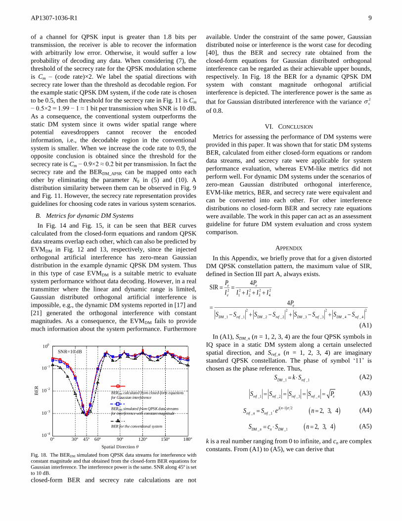
Fig. 18. The BERDM simulated from QPSK data streams for interference with

constant magnitude and that obtained from the closed-form BER equations for Gaussian interference. The interference power is the same. SNR along 45º is set

to 10 dB.

closed-form BER and secrecy rate calculations are not

available. Under the constraint of the same power, Gaussian

distributed noise or interference is the worst case for decoding

[40], thus the BER and secrecy rate obtained from the

closed-form equations for Gaussian distributed orthogonal

interference can be regarded as their achievable upper bounds,

respectively. In Fig. 18 the BER for a dynamic QPSK DM

system with constant magnitude orthogonal artificial

interference is depicted. The interference power is the same as

that for Gaussian distributed interference with the variance 2

v

of 0.8.

VI. CONCLUSION

Metrics for assessing the performance of DM systems were

provided in this paper. It was shown that for static DM systems

BER, calculated from either closed-form equations or random

data streams, and secrecy rate were applicable for system

performance evaluation, whereas EVM-like metrics did not

perform well. For dynamic DM systems under the scenarios of

zero-mean Gaussian distributed orthogonal interference,

EVM-like metrics, BER, and secrecy rate were equivalent and

can be converted into each other. For other interference

distributions no closed-form BER and secrecy rate equations

were available. The work in this paper can act as an assessment

guideline for future DM system evaluation and cross system

comparison.

APPENDIX

In this Appendix, we briefly prove that for a given distorted

DM QPSK constellation pattern, the maximum value of SIR,

defined in Section III part A, always exists.

2 2 2 2 2

1 2 3 4

2 2 2 2

_1 _1 _ 2 _ 2 _3 _3 _ 4 _ 4

4SIR

4

e e

e

e

DM ref DM ref DM ref DM ref

P P

I I I I I

P

S S S S S S S S

(A1)

In (A1), SDM_n (n = 1, 2, 3, 4) are the four QPSK symbols in

IQ space in a static DM system along a certain unselected

spatial direction, and Sref_n (n = 1, 2, 3, 4) are imaginary

standard QPSK constellation. The phase of symbol ‘11’ is

chosen as the phase reference. Thus,

_1 _1DM refS k S (A2)

_1 _ 2 _3 _ 4ref ref ref ref eS S S S P (A3)

1 2

_ _1 2, 3, 4j n

ref n refS S e n

(A4)

_ _1 2, 3, 4DM n n DMS c S n (A5)

k is a real number ranging from 0 to infinite, and cn are complex

constants. From (A1) to (A5), we can derive that

AP1307-1036-R1 10

2 2 22 2 3 2

2 3 3

2

2 2

2 2 2

2 2

3 3 3

2 2

4 4 4

2

41

SIR

2 1

2 cos 1

2 cos 1

2 cos 1

4

j j jk k c e k c e k c e

k k

c k c k

c k c k

c k c k

a k b k

(A6)

αn (n = 2, 3, 4) is the angle between cn and ej(n-1)π/2

. Since 2 2 2

2 3 41 0a c c c

(A7)

The minimum value of 4

SIR exists when k belongs to (0, + ).

In other words, the maximum value of SIR always exists. The

corresponding value of eP , with which the maximum SIR is

reached, can be obtained via (A2) and (A3).

ACKNOWLEDGMENT

The authors would like to thank Dr. Youngwook Ko for

useful discussions. They would also like to thank the

anonymous reviewers and editors for their valuable comments

and suggestions.

REFERENCES

[1] X. Li, J. Hwu, and E. P. Ratazzi, “Using antenna array redundancy and

channel diversity for secure wireless transmissions,” Journal of

Communications, vol. 2, no. 3, pp. 24–32, May 2007. [2] Y. Hwang and H. C. Papadopoulos, “Physical-layer secrecy in AWGN

via a class of chaotic DS/SS systems: analysis and design,” IEEE Trans.

Signal Processing, vol. 52, no. 9, pp. 2637–2649, Sept. 2004. [3] Yi-Sheng Shiu, Shih-Yu Chang, Hsiao-Chun Wu, S. C. Huang, and

Hsiao-Hwa Chen, “Physical layer security in wireless networks: a tutorial,” IEEE Trans. Wireless Commun., vol. 18, pp. 66–74, 2011.

[4] M. Bloch and J. Barros, Physical-Layer Security from Information Theory

to Security Engineering. Cambridge University Press, Oct. 2011. [5] A. Babakhani, D. B. Rutledge, and A. Hajimiri, “Transmitter

architectures based on near-field direct antenna modulation,” IEEE J.

Solid- State Circuits, vol. 43, no. 12, pp. 2674–2692, Dec. 2008. [6] A. Babakhani, D. Rutledge, and A. Hajimiri, “Near-field direct antenna

modulation,” IEEE Microw. Mag., vol. 10, pp. 36–46, 2009.

[7] A. H. Chang, A. Babakhani, and A. Hajimiri, “Near-field direct antenna modulation (NFDAM) transmitter at 2.4GHz,” in Antennas and

Propagation Society International Symposium, 2009 IEEE, 2009, pp. 1–

4. [8] M. P. Daly and J. T. Bernhard, “Directional modulation technique for

phased arrays,” IEEE Trans. Antennas Propagat., vol. 57, pp. 2633–2640,

2009. [9] M. P. Daly and J. T. Bernhard, “Beamsteering in pattern reconfigurable

arrays using directional modulation,” IEEE Trans. Antennas Propagat.,

vol. 58, pp. 2259–2265, 2010. [10] M. P. Daly, E. L. Daly, and J. T. Bernhard, “Demonstration of directional

modulation using a phased array,” IEEE Trans. Antennas Propagat., vol.

58, pp. 1545–1550, 2010. [11] H. Shi and T. Alan, “Direction dependent antenna modulation using a two

element array,” in Proc. 5th Eur. Conf. on Antennas and Propagation,

2011, pp. 812–815. [12] H. Shi and T. Alan, “An experimental two element array configured for

directional antenna modulation,” in Proc. 6th Eur. Conf. on Antennas and

Propagation, 2012, pp. 1624–1626. [13] H. Shi and T. Alan, “Enhancing the security of communication via

directly modulated antenna arrays,” IET Microw., Antennas Propag., vol.

7, no. 8, pp. 606–611, June 2013.

[14] Y. Ding and V. Fusco, “BER driven synthesis for directional modulation

secured wireless communication,” International Journal of Microwave and Wireless Technologies. Available: http://dx.doi.org/10.1017/S175-

9078713000913

[15] Y. Ding and V. Fusco, “Directional modulation transmitter radiation pattern considerations,” IET Microw., Antennas Propag. Available:

http://dx.doi.org/10.1049/iet-map.2013.0282

[16] Y. Ding and V. Fusco, “Directional modulation transmitter synthesis using particle swarm optimization,” in Antennas and Propagation

Conference (LAPC), Loughborough, UK, Nov. 11–12 2013, pp. 500–503.

[17] Y. Zhang, Y. Ding, and V. Fusco, “Sidelobe modulation scambling transmitter using Fourier Rotman lens,” IEEE Trans. Antennas Propagat.,

vol. 61, pp. 3900–3904, 2013.

[18] Y. Ding and V. Fusco, “Sidelobe manipulation using Butler matrix for 60 GHz physical layer secure wireless communication,” in Antennas and

Propagation Conference (LAPC), Loughborough, UK, Nov. 11–12 2013,

pp. 61–65. [19] R. Negi and S. Goel, “Secret communication using artificial noise,” in

Vehicular Technology Conference, 2005. VTC-2005-Fall. 2005 IEEE

62nd, 2005, pp. 1906-1910. [20] S. Goel and R. Negi, “Guaranteeing secrecy using artificial noise,” IEEE

Trans. Wireless Commun., vol. 7, pp. 2180–2189, 2008.

[21] Y. Ding and V. Fusco, “A vector approach for the analysis and synthesis of directional modulation transmitters,” IEEE Trans. Antennas Propagat. Available: http://dx.doi.org/10.1109/TAP.2013.2287001

[22] T. Hong, Mao-Zhong Song, and Y. Liu, “Dual-beam directional modulation technique for physical-layer secure communication,” IEEE

Antennas Wireless Propag. Lett., vol. 10, pp. 1417–1420, 2011. [23] C. A. Balanis, Antenna Theory: Analysis and Design, 3rd ed. New York:

Wiley, 2005, pp. 27–29.

[24] N. Valliappan, A. Lozano, and R. W. Heath, “Antenna subset modulation for secure millimeter-wave wireless communication,” IEEE Trans.

Commun., vol. 61, pp. 3231–3245, Aug. 2013.

[25] M. P. Daly, “Physical layer encryption using fixed and reconfigurable antennas,” Ph.D. dissertation, Dept. Electrical and Computer Eng.,

University of Illinois at Urbana-Champaign, 2012.

[26] S. Forestier, P. Bouysse, R. Quere, A. Mallet, J.-. Nebus, and L. Lapierre, “Joint optimization of the power-added efficiency and the error-vector

measurement of 20-GHz pHEMT amplifier through a new dynamic

bias-control method,” IEEE Trans. Microw. Theory Techniques, vol. 52, pp. 1132–1141, 2004.

[27] R. A. Shafik, S. Rahman, and AHM Razibul Islam, “On the extended

relationships among EVM, BER and SNR as performance metrics,” in Proc. Int. Conf. on Electrical and Computer Engineering, 2006, pp. 408–

411.

[28] A. D. Wyner, “The wire-tap channel,” Bell Sys. Tech. Journ., vol. 54, no. 8, pp. 1355–1387, Oct. 1975.

[29] I. Csiszar and J. Korner, “Broadcast channels with confidential

messages,” IEEE Trans. Inf. Theory, vol. 24, pp. 339–348, 1978. [30] Shunsuke Ihara, Information Theory for Continuous systems. World

Scientific Publishing Co. Pte. Ltd., 1993, pp. 177–184.

[31] Ke-Lin Du and M. N. S. Swamy, Wireless Communication Systems from RF Subsystems to 4G Enabling Technologies. Cambridge University

Press, 2010, pp. 571–575.

[32] G. Ungerboeck, “Channel coding with multilevel/phase signals,” IEEE Trans. Inf. Theory, vol. IT–28, pp. 56–67, Jan. 1982.

[33] Philip Edward McIllree, 1995: Channel Capacity Calculations for M-ary

N-dimensional Signal Sets. M.E. thesis in Electronic Engineering, The University of South Australia.

[34] J. P. Aldis and A. G. Burr, “The channel capacity of discrete time phase

modulation in AWGN,” IEEE Trans. Inf. Theory, vol. 39, pp. 184–185, Jan. 1993.

[35] C. E. Shannon, “A mathematical theory of communication,” Bell Syst.

Tech. J., vol. 27, pp. 379–423, July 1948. [36] Thomas M. Cover and Joy A. Thomas, Elements of Information Theory.

2nd ed. John Wiley&Sons, INC., 2006, pp. 261–264.

[37] A. H. Stroud, Approximate Calculation of Multiple Integrals.

EnglewoodCliffs, New Jersey, Prentice-Hall, 1971, pp. 23–52.

[38] Vladimir Ivanovich Krylov (Translated by A. H. Stroud), Approximate

Calculation of Integrals. Macmillan, New York, 1962, pp. 129–130 and pp. 343–346.

[39] S. T. Brink, “Convergence behavior of iteratively decoded parallel

concatenated codes,” IEEE Trans. Commun., vol. 49, no. 10, pp. 1727–1737, Oct. 2001.

http://dx.doi.org/10.1049/iet-map.2013.0282

AP1307-1036-R1 11

[40] Shunsuke Ihara, Information Theory for Continuous systems. World

Scientific Publishing Co. Pte. Ltd., 1993, pp. 53–54.

establishing metrics for assessing the performance of ... · pdf filepersonal use of this...

Documents