establishing parking generation rates for selected land uses in … · 2016. 4. 18. · my...
TRANSCRIPT

An-Najah National University
Faculty of Graduate Studies
Establishing Parking Generation
Rates for Selected Land Uses in the
West Bank
By
Jamil Mohammad Jamil Hamadneh
Supervisor
Dr. Khaled Al-Sahili
This Thesis is Submitted in Partial Fulfillment of the Requirements for
the Degree of Master of Science in Civil Engineering, Faculty of
Graduate Studies, An-Najah National University, Nablus, Palestine.
2015


III
1 Dedication
بسن اهلل الزحوي الزحين
الوؤهى( رسل عولكن )قل اعولا فسيز الل
My beloved parents, my brothers, my sisters
My Holy Homeland Palestine

IV
2 Acknowledgement
Firstly, I would like to express my sincere gratitude to my advisor
Dr. Khaled Al Sahili for the continuous support of my M.Sc. study, for his
patience, motivation, and immense knowledge. His encouragement,
guidance and invaluable suggestions enabled me to develop an
understanding of the subject. I could not have imagined having a better
advisor and mentor for my M. Sc. study.
I do appreciate my friends, colleagues, students, lecturers, who
assisted, advised, and supported my research. Especially, I need to express
my gratitude and deep appreciation to Eng. Muath Najjar, Eng.
Mohammad Dwikat, and Eng. Khaled Assi whose experience, knowledge,
and wisdom have supported, and enlightened me over the thesis period.
Special thanks for Eng. Ahmad Mustafa for his participation and
cooperation in data collection process.
Last but not the least; I would like to thank my family: my parents
and my brothers and sister for supporting me spiritually throughout writing
this thesis.
All praise and glory be to Allah for his limitless help and guidance. Peace
pleasing of Allah be upon His prophet Mohammed.


VI
4 Table of Contents
1 Dedication ____________________________________________________________ III
2 Acknowledgement _____________________________________________________ IV
3 Declaration ____________________________________________________________ V
4 Table of Contents ______________________________________________________ VI
List of Abbreviations _____________________________________________________ XIV
Abstract________________________________________________________________ XVI
5 Chapter One ___________________________________________________________ 1 5.1 Background ________________________________________________________ 1
5.2 Research Problem ___________________________________________________ 3
5.3 Justification and Research Significance __________________________________ 4
5.4 Thesis Objectives ___________________________________________________ 6
5.5 Study Area ________________________________________________________ 7
5.6 Thesis Outline ______________________________________________________ 7
6 Chapter Two ___________________________________________________________ 9 6.1 General Overview ___________________________________________________ 9
6.2 Review of Parking Studies ____________________________________________ 9
6.2.1 International Studies ____________________________________________ 10
6.2.2 Regional Studies ________________________________________________ 29
6.2.3 Local Studies ___________________________________________________ 31 6.3 Summary and Discussion ____________________________________________ 33
7 Chapter Three ________________________________________________________ 35 7.1 Background _______________________________________________________ 35
7.2 Data Collection Procedure ___________________________________________ 35
7.2.1 Desk Review ___________________________________________________ 36
7.2.2 Selection of Variables ____________________________________________ 36
7.2.3 Sample Size Determination _______________________________________ 36
7.2.4 Sites Selection __________________________________________________ 37
7.2.5 Classification of Land Uses _______________________________________ 38
7.2.6 Data Collection Forms Design _____________________________________ 39
7.2.7 Interviews _____________________________________________________ 39
7.2.8 Count Periods and Durations _____________________________________ 40
7.2.9 Filtering/Screening ______________________________________________ 41
7.2.10 Parking Accumulation Survey Counts ______________________________ 41
7.2.11 Data Aggregation _______________________________________________ 42 7.3 Data Analysis Process _______________________________________________ 42
7.3.1 Maximum Average Parking Accumulation __________________________ 42
7.3.2 Test of Normality _______________________________________________ 44
7.3.3 Overview of Simple Linear Regression _____________________________ 45
7.3.4 Rates _________________________________________________________ 47
7.3.5 Goodness of Fit: Coefficient of Determination (R Square) _____________ 47
7.3.6 Statistical Tests _________________________________________________ 48 7.4 Software _________________________________________________________ 49
7.5 Developing Parking Generation Model _________________________________ 49
7.6 Models Verification and Validation ____________________________________ 49
7.7 Selection of Study Area and its Characteristics ___________________________ 51
8 Chapter Four _________________________________________________________ 52 8.1 Study Area _______________________________________________________ 52

VII 8.2 Sample Size_______________________________________________________ 52
8.3 Types of Data Collection ____________________________________________ 53
8.4 Survey Forms _____________________________________________________ 54
8.5 Field Survey ______________________________________________________ 55
8.6 Data Aggregation __________________________________________________ 55
8.6.1 Residential Land Use ____________________________________________ 55
8.6.2 Office Land Use Class ___________________________________________ 60
8.6.3 Retail Land Use ________________________________________________ 63 8.7 Parking Accumulation ______________________________________________ 66
8.7.1 Residential Land Use ____________________________________________ 67
8.7.1 Office Land Use ________________________________________________ 68
8.7.2 Retail Land Use ________________________________________________ 70
9 Chapter Five __________________________________________________________ 73 9.1 Introduction _______________________________________________________ 73
9.2 Simple Regression Analysis __________________________________________ 73
9.2.1 General Form of Parking Generation Models/ Equations ______________ 74 9.3 Data Analysis _____________________________________________________ 75
9.3.1 Descriptive Statistics ____________________________________________ 76
9.3.2 Residential Land Use ____________________________________________ 77
9.3.3 Office Land Use ________________________________________________ 98
9.3.4 Retail Land Use _______________________________________________ 109 9.4 Models Verification and Validation ___________________________________ 113
10 Chapter Six __________________________________________________________ 119 10.1 Introduction ______________________________________________________ 119
10.2 Conclusions ______________________________________________________ 120
10.3 Recommendations _________________________________________________ 122
References ______________________________________________________________ 125
11 Appendix (A): Data Collection Form _____________________________________ 131 1. Offices & Retail __________________________________________________ 131
2. Residential (Apartment, Detached, and Attached Housing) _________________ 132
12 Appendix (B): Parking Count Sheet _____________________________________ 133
13 Appendix (C): Descriptive Statistic ______________________________________ 134
14 Appendix (D): Models and Rates Sheet ___________________________________ 142
15 Residential Land Use __________________________________________________ 142 a. Attached Housing Class ____________________________________________ 142
b. Detached Housing Class ____________________________________________ 146
c. Apartment Housing Class ___________________________________________ 150
16 Office Land Use ______________________________________________________ 156 a. General Office Class _______________________________________________ 156
b. Institutional Office Class ___________________________________________ 168
c. Government Office Class ___________________________________________ 180
17 Retail Land Use ______________________________________________________ 192 a. Supermarket Retail Class ___________________________________________ 192
b. Strip Retail Class _________________________________________________ 195
Appendix (E): Residual Plots ______________________________________________ 198 18 198
19 Sample of Residual Plots ___________________________________________ 198
Attached Housing Land Use ____________________________________________ 198 20 AM Period_______________________________________________________ 198

VIII 25 Detached Housing Land Use Class _______________________________________ 203 26 Power Relationship ________________________________________________ 203
31 Apartment Housing Land Use Class _____________________________________ 207 32 AM Period_______________________________________________________ 207
36 PM Period _______________________________________________________ 210
40 212
41 Office Land Use ______________________________________________________ 213
42 General Office Land Use Class __________________________________________ 213 43 Peak Period ______________________________________________________ 213
48 AM Period_______________________________________________________ 218
53 PM Period _______________________________________________________ 222
58 Institutional Office Class _______________________________________________ 226 59 Peak ____________________________________________________________ 226
64 AM Period_______________________________________________________ 230
69 PM Period _______________________________________________________ 234
74 Government _________________________________________________________ 237 75 Peak Period ______________________________________________________ 237
80 AM Period_______________________________________________________ 241
85 PM Period _______________________________________________________ 245
90 248
91 Retail Land Use ______________________________________________________ 249
92 Peak of Development/s_________________________________________________ 249 93 Supermarket Retail Class ___________________________________________ 249
97 Strip Retail Class _________________________________________________ 253
101 Appendix (F): Part of Palestinian Regulations ______________________ 256
Vitae __________________________________________________________________ 262

IX
List of Tables
Table 4-1: Collected Data about Attached Housing Land Use (AH) ___ 57
Table 4-2: Collected Data about Detached Housing Land Use (DH) ___ 58
Table 4-3: Collected Data about Apartment Housing Land Use (APH) _ 59
Table 4-4: Collected Data about General Office Land Use Class ______ 61
Table 4-5: Collected Data about Institutional Office Land Use Class ___ 61
Table 4-6: Collected Data about Government Office Land Use Class __ 62
Table 4-7: Collected Data about Supermarket Land Use Class ________ 64
Table 4-8: Collected Data about Strip Retail Land Use Class _________ 65
Table 4-9: Collected Data about Shopping Center Land Use Class ____ 66
Table 4-10: Attached Housing Land Use Class Parking Accumulation _ 67
Table 4-11: Detached Housing Land Use Class Parking Accumulation _ 67
Table 4-12: Apartments Housing Land Use Class Parking Accumulation 68
Table 4-13: General Office Class Parking Accumulation ____________ 68
Table 4-14: Institutional Office Class Parking Accumulation _________ 69
Table 4-15: Government Office Class Parking Accumulation ________ 70
Table 4-16: Supermarket Parking Accumultation __________________ 71
Table 4-17: Strip Class Parking Accumulation ____________________ 72
Table 4-18: Shopping Center Class Parking Accumulation __________ 72
Table 5-1: Parking Generation Sheet Form _______________________ 76
Table 5-2: Descriptive Statistics for No. of Inhabitants of AH ________ 77
Table 5-3: Descriptive Statistics for No. of Occupied AH Units ______ 78
Table 5-4: AH Land Use Class Regression Analysis Parameters ______ 79
Table 5-5: AH Simple Linear Regression ANOVA Table ___________ 80

X
Table 5-6: AH Simple Linear Regression Coefficients ______________ 80
Table 5-7: Critical Values of the t - Distribution (Z) ________________ 86
Table 5-8: Parking Generation Models for AH Residential Land Use Class
in AM and PM Periods ___________________________ 87
Table 5-9: Parking Generation Rates for AH Residential Land Use Class in
AM and PM Periods _____________________________ 88
Table 5-10: Parking Generation Models for DH Residential Land Use
Class in AM and PM Periods _______________________ 90
Table 5-11: Parking Generation Rates for DH Residential Land Use Class
in AM and PM Periods ____________________________ 91
Table 5-12: Parking Generation Models for APH Residential Land Use
Class on AM and PM Periods _______________________ 93
Table 5-13: Parking Generation Rates for APH Residential Land Use Class
on AM and PM Periods____________________________ 94
Table 5-14: Parking Generation Models/Rates of Resdential Land Use _ 95
Table 5-15: Recommended Parking Generation Models/Rates of Resdential
Land Use _______________________________________ 96
Table 5-16: The Obtained Parking Generation Models/Rates of Residential
Land Use vs.ITEModels/Rates * ____________________ 97
Table 5-17: Parking Generation Models for Office Land Use Classes Based
in Peak Parking of Development ____________________ 99
Table 5-18: Parking Generation Rates for Office Land Use Classes Based
in Peak Parking of Development ___________________ 100

XI
Table 5-19: Parking Generation Models for Office Land Use Classes Based
in AM Peak Accumulation ________________________ 102
Table 5-20: Parking Generation Rates for Office Land Use Classes Based
on AM Peak Accumulation ________________________ 103
Table 5-21: Parking Generation Models for Office Land Use Classes Based
on PM Peak Accumulation ________________________ 104
Table 5-22: Parking Generation Rates for Office Land Use Classes Based
on PM Peak Accumulation ________________________ 105
Table 5-23: Parking Generation Models/Rates of Office Land Use ___ 107
Table 5-24: Recommended Parking Generation Models/Rates of Office
Land Use _____________________________________ 108
Table 5-25: Parking Generation Models for Retail Land Use Classes Based
on Peak Demand of Development __________________ 110
Table 5-26: Parking Generation Rates for Retail Land Use Classes Based
on Peak Demand of Development __________________ 111
Table 5-27: Parking Generation Rates for Shopping Center Land Use Class
_____________________________________________ 111
Table 5-28: Parking Generation Models/Rates of Retail Land Use ____ 112
Table 5-29: Recommended Parking Generation Models/Rates of Retail
Land Use _____________________________________ 112
Table 5-30: Models Verification of DH Class ____________________ 114
Table 5-31: Models Verification of Government Office Class _______ 115
Table 5-32: Models Verification of Strip Retail Class _____________ 115
Table 5-33: Rates Verification of APH and DH Classes ____________ 116

XII
Table 5-34: Rates Verification of Government Office Class _________ 117
Table 5-35: Rates Verification of Strip Retail Class _______________ 118

XIII
List of Figures
Figure 1.1: Study Area _______________________________________ 8
Figure 2.1: Average Peak Period Parking Demand vs. Dwelling Units (ITE,
2010). __________________________________________ 12
Figure 3.1: Flow Chart of Data Collection Process
_______________________________________________ 43
Figure 3.2: Flow chart of Data Analysis Process __________________ 50
Figure 5.1: Model Plot of Parking Demand (AM) vs. No. of Occupied
Houses _________________________________________ 81
Figure 5.2: Model Plot of Parking Demnd (AM) vs. No. of Inhabitants _ 82
Figure 5.3: Residual Normality Plot ____________________________ 84
Figure 5.4: Distribution of Residuals around Mean ________________ 85

XIV
List of Abbreviations AH Attached housing class
AM Morning period
ANOVA Analysis of variance
APH Apartment housing class
B1 Slope (coefficient)
B0 Intercept (constant)
CBD Central business district
CV Coefficient of variation
df Degree of freedom (N-1)
DH Detached housing class (villas/ separate houses)
DU Dwelling unit
EA Engineers Association
F-Test Statistical test has F distribution under H0
GFA Gross floor area
GLA Gross leasable area
GLFA Gross leasable floor area
H0 Null hypothesis
H1 Alternative hypothesis
ITE Institute of Transportation Engineers
LGU Local government unit
Ln Natural logarithm
MoLG Ministry of Local Government
MS Mean square error
N Sample size
NZ New Zealand
P Parking demand (passenger car)
PM Afternoon period
P value The probability of type one error used
R Coefficient of correlation
R2 Coefficient of determination
RMSE Root mean square error (standard error of the estimate)
SA Site area
Sig Significant
SPSS Statistical Package for the Social Sciences
SS Sum of squares
Std Standard deviation
TIS Traffic impact study
TRICS Trip Rate Information Computer System
TSM Transportation systems management
T-Test Statistical hypothesis test, in which the test statistic follows a
Student's t-distribution if the null hypothesis is supported.
UAE United Arab Emirates
UK United Kingdom
USA United States of America
Weekdays Normal days (all days of week except the weekend, first day and last

XV day of calendar days)
X1 Independent variable
єi: Random error
σ Sigma; standard deviation

XVI
Establishing Parking Generation Rates for Selected Land Uses
in the West Bank Cities
By
Jamil M. J. Hamadneh
Supervisor
Dr. Khaled Al-Sahili
Abstract
Estimating parking demand in Palestine needs more oriented studies
towards parking generation to enrich transportation planning, design and
management by valuable information. The available local studies are
partial studies and not based on comprehensive specialized studies.
Furthermore, using regional or international models and rates of parking
demand may not be appropriate for Palestine. This research is conducted to
establish reliable reference for provision of parking supply for three major
types of land uses, which are residential, office, and retail land uses.
Seventy three sites of different land uses were selected through field
investigations, interviews, and availability of information for each site.
These sites cover all the targeted land use types and their classes (three
classes for each type).The study covered all main cities in the West Bank.
Data collection was conducted manually, which contains site
characteristics and average of two days of parking counts during three
periods (AM, PM, and Peak of the Development).
The analysis of the attained data produced several parking models and rates
that might be used as local specifications for parking demand and supply of

XVII
the three selected land uses. Following the American Institute of
Transportation Engineers procedure, simple linear or logarithmic/power
model forms were investigated.
The produced models have various levels of statistical significance for
identifying the required parking spaces for a current and proposed
development.
The developed models are applicable in the peripheral areas of the cities.
Fifty six models and rates were produced with variable accuracy. Good
statistical models and rates were summarized and highlighted for each type
of land use in tables. Parking generation models with good statistical
significance (R2, etc.) were recommended, otherwise, parking generation
rates are recommended. Simple linear regression, natural logarithmic linear
regression and power were the forms of the recommended models for the
studied land uses.
Therefore, the parking demand of residential, office, retail land uses with
the same characteristics can be identified based on the produced models
and rates. This thesis forms the first step of a future Palestinian “Parking
Generation Manual” that will contain various local land use types, as well
as guidance for the Ministry of Local Government requirements of parking
spaces for various developments.

1
5 Chapter One
Introduction
5.1 Background
Many states around the world have published trip and parking generation
rates/equations in multi-forms such as books, manuals, handbooks, etc.,
and as a result, they produced trip and parking generation rates/equations
that have been used in many areas of planning and for the support of the
preparation of Traffic Impact Studies (TIS). Trip and parking generation
contributes in the formation of urban areas (Urban Morphology) and
supports the decision makers in the planning of the urban areas. For
example, changing the land use pattern of specific area from residential to
commercial will affect the road network system, but at what level this
effect will be? Trip and parking generation rate for each type of land use
will assist in making decisions through conducting TIS and notice the
effects on the adjacent road network system.
The transportation planning system in Palestine does not have a
comprehensive policy or strategy for providing parking spaces for different
land use types. Therefore, there should be clear. Policies and strategies,
which could assist in building better transport mobility and accessibility at
major movements in different areas of cities and contribute in making
planning decisions.

2
In addition to a few studies that deal with parking generation, Palestine has
a law that deals with operational issues of parking spaces called "Traffic
Laws No. 5 for year 2000" (Ministry of Transport, 2005).
The State of Palestine has some standards/regulations for parking spaces
required for different types of developments, and these standards were set
by municipalities, the Ministry of Local Government (MoLG), and
Engineers Association (EA). These standards are not based on specialized
studies and may not consider the detailed characteristics of land use types.
Other operational studies were prepared by Palestinian government that
deals with parking operation and management rather than parking
provision. Therefore, Palestine does not have any partially or completed
parking generation rates/equations in the form of a manual or a book. On
the other hand, MoLG has set and updated parking requirements for
various developments, and these requirements have been used by engineers
for design.
In this study parking generation for residential, retail, and office land uses
is investigated.
The available parking generation documents that were published around
the world may not be compatible with local patterns in Palestine due to
different conditions and environment.

3
5.2 Research Problem
Traffic is still growing every year in the road network as a product of
several factors such as economic, technology, population growth, etc. The
traffic volumes on road network are increasing due to the creation of new
developments or changing the land use type of specific developments from
one to another without changing parking supply, and some of these actions
are taken without precautions or proper traffic impact studies. The
available parking regulations, which are used in urban development, are
outdated and these regulations did not depend on a specific study. As a
result, the transportation network is congested and needs quick actions due
to the increased parking demand generated from land uses. In urban areas
of Palestine, especially in major cities in the West Bank, has been suffering
from traffic congestion at critical locations, and one of many causes of
congestion is the extensive use of on-street parking by adjacent land uses.
Therefore, estimating the parking generation for each type of land use
(development) will provide for the evaluation of the parking spaces
required because different land uses have different parking demands. The
decision makers or transport planners will assess the impacts of
construction of new development on the road network at the preliminary
stage (i.e. before development construction) and decide on the mitigation
measures based on anticipated impacts.

4
5.3 Justification and Research Significance
Parking generation has helped professionals working in transportation and
urban planning due to its effects and impacts in managing the traffic and
guiding the urban/transport planners in making decisions about land use
patterns of the city based on the amount of parking demand generated by
specific land uses. Adequate provision of off-street parking discourages on-
street parking and improves safety and the level of service.
This work has been done in several cities, states, provinces, etc. around the
world, but in Palestine it is still lacking of a comprehensive study. Studies
conducted abroad (i.e., USA, Abu Dhabi, UK, etc.) cannot be applied as a
whole locally due to major differences in factors like travel habits,
economic size, people, developments types, sizes, Israeli occupation, and
others. Therefore, it is necessary to conduct and establish local parking
generation rates/equations for Palestinian cities in order to form the initial
stage in making local parking generation guide, manual, or book.
This research supports and enriches planners with information, but also it
fills the gap in the planning and engineering process. And this research
forms the base point for planners to decide about proposed/new
development, and it assists in preparing reliable Traffic Impact Studies
(TIS), where parking characteristics are key input data to TIS. Therefore,
producing local parking generation rates for the Palestinian cities will
fulfill one of the important requirements of TIS and engineering designs.

5
Main cities in Palestine suffer from congestion at critical sites due to
improper planning for parking facilities regarding new developments or
identifying the type of suitable land use. As a result, this guides the
transportation planners in managing the transportation system and assists
them in their planning decisions. Furthermore, this thesis assists the key
stakeholders (i.e., government agencies and municipalities) to
institutionalize TIS and update any available regulations regarding parking
facilities.
The existing of major developments such as: residential, shopping centers,
hotels, hospitals, supermarkets, and others need parking facilities such as
on-street and off street parking. These parking areas affect traffic on
roadways; roadways are able to accommodate limited number of parking
due to the limited available capacity and space as well as other factors.
Conducting parking generation analysis will enable the decision makers to
take in their accounts the traffic issues and the capacity of road network
through preparing policies related to institutionalizing TIS. This will create
a room to determining regulations for buildings in different land uses and
as well as a cost sharing mechanism (i.e., impact of parking supply on the
network ought to require investors to contribute to mitigation measures)
that will assist the agencies in developing their cities.
In summary, this research establishes the ground for estimating the number
of parking spaces required for each land use type as well as assists in
developing strategies for mitigating their adverse impacts. Therefore, the

6
process will make stakeholders get involved in decision making by
participating in finding solutions and conducing proper actions.
5.4 Thesis Objectives
The following is the main objective of this thesis is to establish a parking
generation document to be used in predicting the needs of three main land
use types (residential, office, and retail) for parking spaces.
Whilst, the envisaged outcomes of this thesis are shown below:
Specify limitations of the study for the future research.
Support the transportation planning process and the parking
management through several policies and actions such as TIS.
Develop a new tool that assists in Transportation Systems
Management (TSM).
Provide foreseen results about proposed land use for decision
makers. For example, accepting, rejecting, or demanding
modifications as related to changing or creating new
development/land use in one place.
Support urban planning development and assist the
municipalities and ministries in making planning decisions.
In essence; the output of this study is to evaluate how many spaces are
required for parking for specific land use/development. Developing local

7
parking generation rates or equations for the selected land uses will
contribute to establishing a Palestinian “Parking Generation Manual.”
5.5 Study Area
Urban areas outside the CBDs of cities in the West Bank were selected as a
study area as shown in Figure 5.1. Many sites were studied in almost all
cities in the West Bank. Nablus, Ramallah and Albireh and Hebron were
the main cities among all because they have a lot of diversity in land uses.
5.6 Thesis Outline
The thesis contains the following chapters; introduction which presents
general background, problem definition, and objectives of the research.
Literature review is discussed in chapter two. The methodology is
presented in chapter three, while field survey and data collections are
discussed in chapter four. Data analysis and outputs are presented and
discussed in chapter five. In addition, conclusions and recommendations
are presented in chapter six.

8
Figure 5.1: Study Area
Source: (Ministry of Local Government, 2015)

9
6 Chapter Two
Literature Review
6.1 General Overview
Parking and trip rates/equations are used in evaluating the requirements of
transportation network such as the right of way adjacent to specific land
use or the maximum traffic volume should not be exceeded in the adjacent
street, as well as size of parking for each type of land use. Excessive on-
street parking supply may affect negatively the level of service of roads
network due to the generated obstructions from these parked vehicles.
Furthermore, deficiency in providing sufficient off-street parking spaces
for land uses such as retail and office creates negative economic impacts.
On the other hand, size of parking supply might exhaust roads network and
drop down the level of service to the worst. In essence, estimating parking
generation for different uses absolutely contributes in specifying and
controlling parking supply for each land use, and consequently avoiding
congestion generated by parking.
6.2 Review of Parking Studies
This section provides a review of selected past relevant studies of parking
generation that have been conducted in three levels; international, regional,
and local studies. Historically, many studies around the world have been

10
developed and used. Unfortunately, local studies as researches, manuals,
books, etc. are scarce as shown in the following subsections.
6.2.1 International Studies
International studies are divided into the following sub-sections:
6.2.1.1 North America
The American Institute of Transportation Engineers (ITE) published
several studies about parking generation in different format such as
journals and reports. The most recent report is the 4th
edition of Parking
Generation, which involves 106 land uses. Indeed, the 4th
Edition Parking
Generation report represents a collection of data since 1978.
The 4th
Edition of Parking Generation, which will be called later as "ITE
Parking Generation", involves parking demand observation, time and date
of observation, and independent variables. Parking Generation
demonstrates a reasonable relationship between parking demand and single
independent variable. Previous editions used the average maximum
parking demand ratios in predicting parking demand regardless of some
important factors such as area type. On the contrary, the third and fourth
editions did not use that, but it began to take more factors of estimation
parking demand such as linking data to time and area type. Most of the
data available in the ITE Parking Generation are from suburban sites with
free parking and single use.

11
Parking Generation produced various levels of statistics ranging from poor
to good. For example, when using the gross floor area (GFA) with parking
demand it produces high coefficient of variation; however, when using
number of employees it produces low coefficient of variation. The ITE
concluded that homogeneous data sets or small data sets may produce low
coefficient of variation and this does not mean more reliable relationship.
Statistically reliable data does not cover all sites but it forms a long range
goal. Indeed, average or mean parking demand has been used in Parking
Generation (ITE, 2010).
ITE (2010) provides information and guidelines about site selection,
permissions, procedure, background, and independent variables. The
following are some variables in ITE documents that were used in
predicting parking demand:
Residential: dwelling units, persons, vehicles, acres.
Office: employees, 1,000 square feet (sq. ft.)GFA, acres.
Retail: employees, acres, 1,000 sq. ft. GFA, 1,000 sq. ft.
occupied gross leasable area (GLA), etc.
Shopping Center: 1,000 sq. ft. GFA, employees, % restaurant
space, % entertainment space.
ITE Parking Generation provides models and rates for predicting parking
demand for various land use types, for example on weekday, Low/Mid-rise
Apartment generates 0.59 to 1.94 and 0.66 to 2.5 parked vehicle per

12
dwelling unit (DU) for suburban and urban areas, respectively. Office
Building generates 0.86 to 5.58 and 1.46 to 3.43 parked vehicles per 1000
sq. ft. GFA for suburban and urban areas, respectively. Shopping Center
generates 1.44 to 7.37 parked vehicles per 1000 sq. ft. for non-Friday
weekday (ITE, 2010).Figure 6.1exhibits an example of parking generation
model/equation for Low/Mid-Rise Apartment through average peak period
of weekday in urban area.
The 2nd
Edition of Parking Generation covered only suburban areas, and
the last two editions covered five areas: CBD, central city (not downtown),
suburban center, suburban, and rural. Parking Generation showed that local
conditions and area type can influence parking demand. Parking
Generation introduced the importance of estimation of parking demand
with respect to the ambient temperature (McCourt, 2004).
Figure 6.1: Average Peak Period Parking Demand vs. Dwelling Units (ITE, 2010).

13
Kuah (1991) followed a procedure for estimating parking demand in order
to develop ordinances to regulate parking supply for meeting peak parking
demand for a single use. The author used several factors, including project
size, type of zoning, type and number of persons expected to visit the site,
availability of alternative transportation modes, and the time frame of the
analysis in performing the study. The author proposed a methodology for
estimating parking demand for Mixed Use Developments (MXDs) planned
in jurisdictions with Transportation System Management (TSM) programs
ordinances. The proposed method accounted for potential parking
reductions resulting from the implementation of TSM and the sharing of
parking spaces for MXDS (Kuah, 1991).
The author concluded that the study not only takes into account parking
reductions because of TSM programs, but it also addresses the saving of
spaces because of shared parking among different land uses of the MXDs.
Based on that approach, developers will be able to provide an adequate
number of parking spaces that might vary from the code requirements.
Meyer (1984) published guidelines for obtaining parking generation data.
These guidelines involved site selection, permission, background data,
procedure, and existing data. Each one of these guidelines should be
considered in performing parking generation. The study indicated that it is
important to take permission from the owner/manager of prospective
survey site. Procedure for conducting parking occupancy count at each site
should be counted at the time of peak parking demand, and variation of

14
peak parking demand throughout the time horizon should be studied as
well (Meyer, 1984). In addition, the author provided guidelines, and these
were taken into consideration in second, third, and fourth edition of the ITE
Parking Generation.
Gattis et al (1995) studied parking generation at a selected type of schools,
which were elementary schools. The authors addressed the issues
accompanying the generated traffic congestion that occurred on the
surrounding streets at school's beginning and dismissal. The authors
presented methods to predict the parking demand during this "school rush-
hour". Therefore, several factors were studied such as location of school
with respect to different types of roads classes (i.e. collector, local, etc.).
Predictive models were developed based on variables that local officials
could easily estimate or find in common documents, such as census data.
The author concluded, the provision of adequate parking spaces can reduce
school traffic congestion and enhance traffic safety (Gattis et al., 1995).
Smith (1990) prepared a report to guide users of the second edition of ITE
Parking Generation. The author used factors that contribute to parking
demand, which are related to the characteristics of the sites themselves and
others that are related to the way in which each individual study was
conducted such as availability of transit and time of year. In addition,
possible methods for estimating design level parking demand for rates,
equations, and cumulative distributions were addressed. Some of these

15
methods are parking generation rates and standard deviations, regression
equations, and cumulative distributions.
Moreover, Smith (1990) provided precautions when using ITE Parking
Generation, such as care should be taken in using the data where sample
sizes are small. The regression line is used to estimate total peak parking
occupancy, not the generation rate.
In addition, Smith (1990) provided several tips for users when using the
data from the second edition of Parking Generation such as:
The regression line should not be used for sites where the
independent variable is outside the limits of the data available.
Possible choices include using the generation rate or using the
generation rate computed from the high or low limits of the
regression line.
The occupancy computed from the mean rate can be plotted
on the same graph as the regression line for the purpose of
comparison.
When sample sizes are small, little confidence can be placed.
Smith study (1990) investigated two area types, which were suburban
activity centers and downtown sites. The study found that application of
the output rates/equations can be applied on activity center requires
appropriate allowances for time-of-day variations, multiple stops, etc. The

16
author concluded that this would normally be done only for new
development and where more direct studies and data are unavailable.
Rugger and Gorys (1989) studied the impact of a 90-room hotel to be
added to an existing banquet hall in the City of North York, Ontario,
Canada, focusing primarily on the implications of the project with respect
to its parking requirement.
The authors conducted surveys on five sites, including the subject site.
Two of the sites were major hotels in close proximity to the subject site,
while the other two were industrial/ commercial sites adjacent to the
subject site. The degree of certainty that one can put on these values was
calculated through the 95% confidence of the mean.
Analysis of collected data showed the demand for parking at the two hotels
did not, in any instance during the survey period, ever exceed 75% of the
supply. The present parking capacity at the subject site can accommodate a
hotel operation for 94% of the time; the exception being Saturday evenings
because of the banquet functions. However, this problem already existed
and the owners of the subject site made arrangements with neighbors to
share parking spaces (Ruggero et al., 1989).
Hain et al. (1987) studied parking generation rates developed from
recreational land uses. The authors focused on four recreational land uses
in Colorado: golf courses, athletic clubs, bowling alleys, and ski areas. To

17
simplify the data collection effort, site managers for each land use were
contacted prior to the survey to identify the peak parking demand period.
Several statistics were included in the study such as mean, range, standard
deviation, linear regression equations, and coefficient of determination
(R2),which ranged from (no fit) to 1 (perfect fit). The authors
recommended that additional study of this land use is needed to get more
accurate and reliable estimates (Hain et al., 1987).
Fitzgerald and Halliday (2002) prepared a study for the Northwest
Connecticut regarding parking. Forty two locations were surveyed and
each location was counted twice in two different dates after specifying the
peak period of each location.
Parking occupancy was counted in 10 minutes interval, and area types were
distinguished. Comparison was undertaken between regulations and actual
number of spaces available, and the occupied spaces observed. Square
footage of building space was based on evaluating the number of space
required for specific land use. The study showed that many of parking
areas were underutilized; for example, 11 existing spaces per 1000 sq. ft. of
building area were provided at a general office, and the 3 occupied spaces
were observed, but the national standards set out 5 to 10 spaces per 1000
sq. ft. Therefore, using strategies to reduce the amount of provided parking
in zoning regulations is useful because the results showed the average
percentage of occupied parking spaces was less than 50%, and this percent

18
is smaller than desirable percentage (85 percent to 95 percent). Several
strategies should be followed such making modifications on the existing
standards, and promoting shared parking (Fitzgerald and Halliday, 2002).
Small Office Complexes were not included in ITE Parking Generation.
Therefore, the Montana State University Institute of Transportation
Engineers gathered information on Nopper Technology Building, which is
located in Montana. Traffic tubes were used to collect traffic data on this
development. Estimation of both employees and occupancy in the
development was used. The study was based on the ITE basic forms in
conducting surveys. In three separate times or dates the traffic data were
collected. Square footage was used as independent variable in estimating
parking demand. Different types of modes were included in the results of
this study like trucks, pedestrian, vehicle, and bicycles. Parking rate of 1.67
on average is required for every 1000 sq. ft. GFA (MSU-ITE, 2009).
Rowe et al. (2013) studied the importance of investment in parking
provision. Misunderstanding of variation in parking demand for different
areas (urban, suburban, etc.) leads to overprovision of parking and
increased cost to users that have no need for these facilities.
The author studied the effects of decrease in auto ownership, licensed
drivers, and vehicle miles traveled, especially among young people in
United States. The design of multifamily housing for low rates of vehicle

19
ownership is equally as important as design for suburban conditions where
higher rates of vehicle access are found.
Socio-demographic, housing, and built environment variables have all been
shown to have an impact on residential parking and vehicle availability.
More than 100 factors were developed for data collection and analysis such
as supply and price, property/development characteristics, neighborhood
household characteristics, accessibility, and built form/development
patterns. Sample sizes of 208 sites were assembled, representing various
types of multifamily development around urbanized King County Metro in
the Seattle region. The parking utilization data was correlated with the 100
factors. Factors with higher correlations to parking utilization include the
supply of parking, transit access, walk score, concentrations of people and
jobs, block size transit service, good walk access, and shorter block spacing
have a reasonable potential to provide lower parking supply for a
multifamily residential project (Rowe et al., 2013).
Although each of these factors individually did not exhibit strong
correlation (R2> 0.7), relationships plots were conducted between supply,
transit access, concentration of people and jobs, walk score, and block size
versus observed parking. CBD multifamily parking utilization of 0.51
vehicles per occupied dwelling unit in the sites studied, compared with
suburban 1.18 vehicles per occupied dwelling unit, indicates that better
accommodations/ environment for low- and zero-auto-ownership
households correlates with reduced need for parking. Most important, the

20
research demonstrates that higher supply of parking appears to consistently
correlate with greater parking demand (Rowe et al., 2013).
Rowe et al. (2011) studied the effects of transit availability on the
provision of parking spaces in urban areas. The author examined the
relationship of parking demand and transit service in First Hill– Capitol
Hill (FHCH) and Redmond; two urban centers in King County,
Washington. The results showed a strong relationship between transit
service and parking demand. Parking demand in FHCH was observed to be
0.52 parking spaces per dwelling unit, which was about 50% less than
parking demand observed in Redmond, a growing mixed-use suburban
center, and 50% less than data reported by the ITE.
Two centers were chosen and they represent two contrasting types of
development, an urban and a suburban environment, yet they have the
highest number of multifamily apartment buildings available to study
among all centers in King County Metro in Seattle. To assess parking
demand, eight apartment buildings (four in each urban center) were
selected to conduct parking utilization counts. Property managers at each
development site were contacted to gain permission to use their sites for
this research (Rowe et al., 2011).
Specific criteria were based on filtering and selection of sites such as
permissions from manger or owner of site and occupancy is at least 85
percent. Parking counts were completed during midweek days (Tuesday

21
through Thursday) at the peak parking demand hours for residential land
uses (i.e., from 12:00 to 5:00 a.m.). The results show that parking demand
is lower than the amount supplied in both urban centers, a finding which
suggests that parking is overbuilt. The observed parking demand found in
this study is less than the parking demand data presented in the ITE report
in both urban centers (Rowe et al., 2011).
Gabriel (2010) provided trip generation and parking statistics for Oxford
Plaza in California. This development is categorized as residential land use.
This development is close to commercial area and dozen transit line. Data
collection was done during three weekdays. Person trips and vehicle trips
were identified in the study. Specific parking pricing strategy in area of
development was reflected in this study.
The author concluded the Oxford Plaza does not provide sufficient parking
to encourage using other modes of travel, and despite of that there were a
lot of vehicles parked outside of development (off-street). Therefore,
parking demand is larger than parking supply (Gabriel, 2010).
Fehr and Peers (2008) provided an assessment of the expected parking
demand and peak hour trip generation of the proposed Stanford Hospitals
and Clinics (SHC)/Lucile Packard Children‟s Hospital (LPCH) projects.
The study utilize traffic counts and parking occupancy surveys to define
unique trip generation and parking demand rates for the hospitals as a
whole (inpatient and clinic space) and for certain Welch Road medical

22
office buildings. These rates were applied to the growth plans for the
hospitals, including new inpatient and clinic space, and for a new medical
office building to be located on the Hoover Pavilion site.
The survey data indicated that the hospitals generate traffic and parking
demand at rates that are generally consistent with rates observed at other
large medical centers. The rates were based on the total floor area for
inpatient space and clinics.
Parking industry publications such as “Parking,” published by the ENO
Foundation, recommend that a vacancy factor of 10 to 15 percent be
applied to the calculated parking demand to quantify the needed parking
spaces to meet parking demand. The vacancy factor is needed to ensure
that drivers are able to locate an available parking space without re-
circulating through the parking areas (Le Craw et al., 1946).
The authors conducted traffic counts during the morning (7:00 to 9:00 AM)
and evening (4:00 to 6:00 PM) peak periods for 20 parking areas. These
counts were conducted using either machine counts or tubes (6 driveways)
and manual/person counts (15 driveways). In addition to driveway counts,
peak period occupancy and parking permit surveys were conducted for the
20 parking areas and three on-street locations. Fehr and Peers also
determined the peak hospital parking occupancy, or „demand‟, during both
the mid-morning and mid-afternoon periods. Parking occupancy or demand
is the number of spaces in which vehicles are parked. As a result, the

23
recommended parking demand rates for the hospitals and medical office
space were determined (Fehr, 2008).
Ornstein (1966) indicated that in residential area there are two points that
should be considered; providing adequate parking spaces plus the place of
parking with respect to developments such as on street. The author studied
the parking demand for the inhabitants‟ vehicles ownership rather than all
users of parking spaces; for example, visitors, customers, and employees.
Ornstein concluded the availability of mass transit in residential area does
not affect the parking spaces. The author presented three factors to alleviate
the problems associated with provision of parking spaces in residential
areas. Zoning ordinances, public power, and providing off-street parking
are factors that could be used as a remedial tools in solving parking
provision problems in existing developments. The author concluded that in
the new development zoning ordinance is the key solution of parking
problem, while in existing developments off-street facilities can be
effective solution for alleviating parking problem (Ornstein, 1966).
6.2.1.2 South America
A new type of land use was discovered in the Portland area, and as a result,
Students in Transportation Engineering and Planning (STEP) (2009)
conducted study in order to include this new type of land use in the ITE
documents. The IKEA is an international, home products retailer with
stores in many countries, and indeed, it is a discount big store. This

24
development has large area store, shopping center, and large parking
spaces for vehicles and bicycles. Pedestrian and bicycle movements were
counted since there was a light rail 500 ft. away from the developments.
This development has its internal trips that prevented distinguishing people
modes of choice. Three separate dates were used to conduct survey counts.
Peaks were identified and documented since the estimation of parking
demand relied on it. Parking accumulation was drawn then the average was
taken as representative one. ITE survey forms were used for conducting the
study (Students in Transportation Engineering and Planning, 2009).
6.2.1.3 Australia
Douglass and Albey (2011) prepared a research study to compare New
Zealand, Australia, UK, and USA information on trip and parking related
to land uses, and reviewed current trip generation survey and data manuals
from these four countries. The research covered surveyed trips to and from
individual sites by all modes of travel, and considered observations from
car park demand surveys. The research considered seasonal traffic and
parking variations and identified the practical parking design demand for a
whole year as the 85th
percentile satisfaction, which is also the 50th
highest
hour. The 85th
percentile was the upper design limit suggested for the site
being considered. Independent variables such as GFA, gross leasable floor
area (GLFA), which is commonly 80% of the GFA, site area (SA),
employees, and activity units were derived from survey process.

25
In residential; primary factors explaining the variation in household trip
generation such as topography, demography, etc. were considered. The
combination of various socio-economic characteristics, student flats, etc.
led to widely varying vehicle use and associated parking demand and
traffic generation. In retail; traditional town center shopping areas
experienced a range of vehicle and pedestrian journeys. In smaller towns
and suburban areas, the proximity of retail areas to residential catchments
means about 10% to 15% of shopping trips are made on foot or by bicycle.
The most practicable unit for most district plans is still spaces per 100 m²
GFA (Douglass and Albey, 2011).
Douglass and Abley (2011) concluded that the designer and planner must
appreciate both the direct effect of the physical features of a site and the
indirect factors such as catchment, competition, and surrounding
transportation systems.
The Roads and Traffic Authority (2002) established a guide that outlined
all aspects of traffic generation considerations relating to developments.
This guide sets out the range of parking demands likely to occur at an
isolated site, recognizing the impact it may have on transport policy and
travel demand. Parking provision should be viewed as the minimum
desirable requirement, while Councils' parking codes are considered to be
minimum mandatory requirements. Roads and Traffic Authority (2002)
conducted traffic counts in both peak periods of which vehicular traffic
occurs (peak of development itself and peak of adjacent road network).

26
The independent variables used were not always suitable for predicting
future traffic generating characteristics of a proposed development. For
example, using employees can be useful for operation studies; not for
future planning studies. The parking provisions recommended are based,
wherever possible, on physical characteristics of the proposed
development, particularly the gross floor area (Roads and Traffic
Authority, 2002).
The Roads and Authority (2002) used 85th
percentile level of demand in
parking demand estimation. For examples, one parking space is required
for each one dwelling unit, and the recommended minimum number of off-
street visitor parking spaces is one space for every 5 to 7 dwellings for
residential land use. About 6.1 parking spaces per 100 sq. m. are required
for GLFA ranging from 0 to 10000 sq. m. In off-street parking GLFA is
preferred to GFA for the shopping center land use category because it
refers most specifically to the factor that generates / attracts trips. As a
guide, about 75% of the GFA is deemed GFLA. However, this percentage
can vary substantially between developments.
Clark (2007) studied trips and parking generation in New Zealand (NZ)
and Australia for the purpose of promotion of practices for sources of
surveyed data that was used in New Zealand and Australia. The study was
undertaken to show the differences, correlations, and similarities in traffic
conditions in UK and NZ land use types. Therefore, a simple system of site
lists linked to data for individual sites was developed in both countries (UK

27
and NZ). Variation through years such as seasonal, weekly, daily, and
hourly factors were included in this study in order to identifying 85%
design hour. Some differences between individual sites within a land use
class were noticed.
However, taking the averages, or more importantly the 85th percentile to
get UK, New Zealand, and probably Australia in the same order is
oriented. Finally; The New Zealand Trips and Parking Database (NZTPD)
is being upgraded and detailed comparisons are being made with Trip Rate
Information Computer System (TRICS) (JMP Consultants Limited., 2013)
to develop the database as well as accuracy and coverage of data (Clark,
2007).
6.2.1.4 Europe
JMP Consultants Limited (1995) studied the provision of parking at food
retailing in order to reduce the trips distance and alleviate the reliance on
car, in addition to providing safe environment through alleviating the
impacts of transportation. Maximum parking demand was recorder for
selected sites of retail in and out of town center. The results indicated the
demand in town center is larger than out of center. Moreover, parking rates
in terms of GFA and retail floor area were computed during three
weekdays which represent the maximum regime. The author also noticed
that there is a relationship between customer visits and maximum parking
demand (JMP Consultants Limited, 1995).

28
JMP Consultants Limited (1995) assessed parking demand in terms of
comparison of existing database of parking demand with existing parking
standards. Six land uses were studied to achieve that comparison. The 85th
percentile was taken as a high value and this value is not rigid; the 50th
percentile and more is suggested. Maximum hourly accumulation of each
site was noted. Base on the gross floor area parking demand ratios were
calculated. The survey was designed to undertake the typical days rather
than peak days to avoid adaptation of peak parking demand. Confidence
level of one standard deviation (std.) from the mean (68%) and two std.
from the mean (94%) were used in data analysis. Seasonal, operational, and
growth in demand factors affected the resultants demand. These factors
were reflected in the 85th
percentile but the results in some instances were
over provision of parking space. Therefore, using lower value to reflect
previous factors was adopted. Comparison of parking demand with existing
standards showed there are many up and down variation values especially
in retail land use.
6.2.1.5 Other Countries
Regidor and Regin (2010) assessed some issues and concerns pertaining to
local trip and parking rates in Philippine. Parking generation in Philippines
used a number of relevant laws pertaining to the provision of off-street
parking for different types of developments, and among these is the
National Building Code (P.D. 1096) of the Republic of the Philippines,
which stipulates the minimum requirements in the number of parking slots

29
per type of development. In this law, developments are classified into
groups and divisions ranging from Group A to Group J; these divisions
summarize several types of land uses such as hotel, residential, industrial,
etc. The study identified several parameters for parking requirements for
such developments such as gross floor area, gross saleable area, floor area
ratio (density), parking slot cost, and distance from the CBD.
However, it is also necessary to point out the importance of estimating
local trip and parking generation rate because ITE trip and parking
generation does not incorporate public transport trips, and it is limited to
vehicle trips that are interpreted as private trips (Regidor et al., 2010).
6.2.2 Regional Studies
The Department of Transport of Abu Dhabi (2012) prepared a manual for
assisting planners, engineers, and developers in estimating the parking and
trip generation rates for several local land uses. These rates have been
obtained through the survey and analysis on nearly 400 different sites
throughout the Emirate.
To ensure sufficient parking with respect to size and location of
development, a specialized process was undertaken in publishing this
manual, which includes site selection, surveys, data analysis and
validation. Parking generation rates that was developed in this manual
covered all types of predominated land uses in Abu Dhabi (Department of
Transportation, 2012).
30
Regional shopping center/mall generates 0.204 resident or employee
parked vehicle, and 2.433 visitor parked vehicle, 0.013 parked
school/company/trucks per 100 sq. m. These rates are based on 4 selected
sites that are well distributed around the study area. Local shopping center
generates 0.107 resident or employee parked vehicle, and 1.204 visitor
parked vehicle, 0.007 parked vehicle school/company/trucks per 100 sq. m.
These rates are based on 5 selected sites that are well distributed around the
study area. In addition, supermarket generates in non-CBD area of Abu
Dhabi 0.949 resident or employee vehicle, and 6.371 visitor parked
vehicle, 0.214 school/company/trucks per 100 sq. m. These rates are based
on 15 selected sites that are well distributed around the study area. Local
government office generates parking rate in Abu Dhabi City of 1.982
vehicles per 100 sq. m. based on sample size of 3. On the other hand,
residential land use was covered in this manual and it was based on the
number of bedroom as an independent variable (Department of
Transportation, 2012).
Al-Masaeid et al. (1999) developed statistical models for estimating
vehicle parking demands of different land uses in Jordan. These land uses
include 53 hospitals, 40 hotels, 42 office buildings, 35 apartment buildings,
21 restaurants, and 17 shopping centers, for a total of 208 sites. The sites
were located in different cities in Jordan, including Amman, Zarqa, and
Irbid. Three criteria were adopted in the selection process. First, each
selected site must have a well-defined parking lot and the parking is not

31
permitted to be used by adjacent land uses. This criterion is important to
determine the peak parking need accurately for the selected land uses only.
Second, the sites of each land use should be located in different cities.
Clearly, this criterion was adopted to increase the domain of inferences.
Third, the parking lot for each site should have an adequate parking supply.
The availability of a sufficient parking supply was judged through field
survey. All selected sites were located outside the CBD‟s. A statistical
model for estimating vehicle parking demand of various land uses in
Jordan was developed.
The developed models had an exponential form, except for models for
restaurants and shopping centers, which had a linear form. The researchers
concluded that compared with the standard values for developed countries,
the parking demands for the investigated land uses in Jordan had lower
rates (Al-Masaeid et al., 1999).
6.2.3 Local Studies
Ordinances were developed and used by the Ministry of Local Government
(MoLG) and municipalities in Palestinian localities regarding provision of
parking supply.
Local small scale studies were conducted by several agencies/
organizations in specific sites in the West Bank such as Traffic Analysis
and Simulation of Al-Ersal Center Project (Al-Sahili, 2010).

32
Al-Sahili (2010) performed parking and traffic counts adjacent to
residential, hotel, office, and shopping / retail center land uses to capture
trips and parking associated with the particular land use. Five sites (land
uses) were surveyed during the AM peak and PM peak periods of atypical
workday. This study provides local trip generation rates and parking
generation rates for the selected developments in the study area. In
addition, the study evaluated the proposed parking supply against the
parking requirements established by MoLG in Palestine. The study
concluded that the local parking requirements may not be suitable for mix
land uses, such as the project of Al-Ersal Center.
Palestinian Buildings Laws and Regulations for Local Government Units
(LGU's) (Ministry of Local Government, 2011)is the only system used
locally by planners, and LGU's for estimating parking requirements for
various land uses. For residential land use class (A, B, and high rise
buildings) one space for each dwelling unit is required. While for Class C,
D, and old city one space for each two dwelling units is required. Retail
land use should provide one space for each 50 square meter of stores and
exhibits one additional space for other uses (other than stores). For each 70
square meter (sq. m.) of office land use one space should be provided.
Appendix (F) shows an extracted table from the Palestinian regulation of
parking spaces provision.

33
6.3 Summary and Discussion
Different studies, reports, and projects were conducted to find parking
generation for various land uses. In summary, the variables used in these
efforts overlap and some of these variables are used in operational
purposes while the others in future or new developments. Types of land
uses not only define what variable should be used in developing parking
generation, but also the case study and the nature participate in defining the
variables. The outputs of some studies were appended by limitations and
precautions when using the developed parking demand generation. Some
studies take different area types but mainly suburban area occupied the
main concern of most of them. Survey tools used in developing parking
generation were interviews, manual counting, and automatic counting
(pneumatic). Some agencies or researchers developed parking generation
rates and compared these with used regulations and codes of their areas.
Parking accumulation of each land use was counted for peak period of
adjacent street, for AM peak, and for PM peak, and this depends upon the
objective of each study.
Linear Regression analysis and the average maximum parking demand
ratio were the major tool in developing parking generation. In addition,
sample size limits the accuracy and power of the output rate or equation
and some studies mentioned that the accuracy developed will be enhanced
in the future by expanding the sample size.

34
In summary, the level of efforts and details were different from one study
to another based on several factors such as time of study, budget,
availability of resources, and the condition of studied area.
The most common independent variables among the reviewed studies will
be investigated. The ITE survey methodology, which is the most common
among these studies, and the time horizons for conducting surveys will be
taken into consideration in this research; specifics of the ITE used in this
research will be presented in later chapters. Furthermore, non-CBD sites or
peripherals of cities will be adopted in the survey in this study.

35
7 Chapter Three
Methodology
7.1 Background
This thesis covers several Palestinian cities in the West Bank. The nature
of cities in the West Bank is different from other cities abroad. The
differences are in terms of size, economic conditions, travel habits, and so
on. These differences lead to the conclusion that the used methodology
may differ a l ittle bit from other research conducted abroad.
Literature review presented that almost all published studies counted
accumulation of parking at different periods of time depending on the
purpose of the study. The ITE has established guidelines for conducting
parking occupancy counts (ITE, 2010). Estimating parking accumulation of
each site by counting parked vehicles at specified intervals and at specific
periods of time is the main purpose of surveying works.
The following sub sections show how the research was conducted.
7.2 Data Collection Procedure
For the purpose of preparing parking generation rates/equations, several
parameters are required at the initial stage in order to get ready for
preparing good data survey forms and traffic counting sheets. The

36
following subsections provide details about main items in the data
collection process:
7.2.1 Desk Review
This process intended for reviewing previous studies related to parking
generation for different types of land uses. Literature review related to
parking generation models or rates was reviewed.
7.2.2 Selection of Variables
Developing of parking generation rates or equations required gathering
information about dependent and independent variables. Therefore, the
selection of independent variables (parameters) depends on the nature of
each land use such as residential land use patterns might use dwelling
units, while retail land use might use number of employees and the same
for office land use patterns. These variables are very important because
parking generation is used to predict parking demand of specific land use
in the form of equations or rates that will be built based on parameters
(independent variables). Therefore, desk review provides several proposed
variables that assist in designing survey form.
7.2.3 Sample Size Determination
Sample size was determined based on the ITE guide, statistical
considerations (example; population size, ranges of data etc.) as well as
some significance levels, and the available resources. Therefore, a

37
minimum of four sites should be provided to conduct analysis and get
useful information as stated by ITE (2010). The higher the sample size, the
better reliability can be reached.
7.2.4 Sites Selection
Searching for suitable sites in each city was done using 2012and 2014
aerial photo of the West Bank. Moreover, the internet websites were
helpful for getting useful information about some sites such as working
days and hours, surrounding areas, nature of its services, location of site,
and so on.
The researcher visited many sites in order to investigate and evaluate
whether the proposed sites are appropriate and meet the set criteria, such as
classification of area (urban, suburban, and rural). ITE (2010) suggested
some guided criteria for selecting sites that enhance the outputs of study,
these are:
Site should be mature (i.e., at least two years old).
Occupancy (i.e., at least 85 percent).
Sites should be clear for the purpose of controlling parking counts on
it.
No abnormal condition besides selected site such as constructions.
Accessible by the surveyors for collecting whole information.

38
ITE stated that sample size of at least four should be analyzed to develop
regression model (McCourt, 2004). This would be appropriate for some
land uses with limited availability.
In addition, evaluation of each site was undertaken in terms of how many
persons (surveyors) are needed to conduct a traffic count, and at what
location they should be. Moreover, meeting and coordinating with the
responsible person of the site and meeting surveyors were conducted
through site visits. In addition, access of site and ability of surveyor to
conduct and control vehicular traffic in and out of the development were
also taken into consideration in the selection process.
Furthermore, selected developments should have single land use because
this research focuses on single land use rather mixed land uses.
7.2.5 Classification of Land Uses
Investigation about the residential, retail, and office land use, and taking
into consideration the local experience and the existing environment in
Palestinian cities, lead to the conclusion that these land uses can be
classified into types, and types could be classified into classes. Residential
land use type can be classified into different classes as attached housing
(AH), detached housing (DH), and apartments (APH). While office land
use was classified based on its nature and services they provided as
general, institutional, and government land use classes. Retail land use was

39
classified to three classes; strip, shopping center, medium to large
supermarket, which is called later supermarket.
7.2.6 Data Collection Forms Design
The type of needed data was determined based on local experience and
international and regional references. Special forms were prepared to
collect necessary information of each selected site and to fulfill the need of
estimating parking generation in terms of the required variables needed
(See Appendix A). Moreover, special counting form was prepared for the
purpose of the parking count survey (Appendix B).
7.2.7 Interviews
Interviews were held with people who have the merit to provide
information about the surveyed development/site. Special interviews were
made with large developments such as Plaza Mall and Jawwal Company to
discuss the research and its objectives. Feedback from these developments
about their requirements to conduct traffic count was taken into
consideration such as coordination with the developments before
conducting the survey.
Permission for conducting the traffic count during specific peak periods of
each site was obtained. Some sites needed two types of permissions; one of
them was local permission, which was requested from the owner/manager

40
and the other permission was security permission from police centers,
ministries, and associations.
Therefore, the communication tools used in getting full information about
sites were: telephone, email, fax, mail, personal interviews, and social
media. These tools were effectively used to improve the accuracy of
counting and getting any future information about sites.
7.2.8 Count Periods and Durations
As stated by ITE, time of counting is connected to the purpose of the study;
from the objectives and outcomes of this research, it is finding peak
periods parking demand of each site during weekdays for the periods of
AM and PM. In addition, time of day in which the adjacent streets of each
site exposed to the highest volume of traffic is recorded in this study.
Therefore, during data collection process information about the peak
movements of vehicles in and out of site was recorded to minimize and
restrict the period of parking count. As a result, two peak periods were
developed, and counts based on 15-minute time interval was used. Time
counting interval is appropriate since ITE used larger interval (I hour) in
order to capture the variation during the whole day (ITE, 2010). Therefore,
as counting interval decreases the probability of detecting the maximum
accumulation increases, especially when the stay duration of parked
vehicle is small.

41
Furthermore, this study covers only the weekdays (Monday, Tuesday, and
Wednesday), and it does not take into account the weekends, holidays, and
any abnormal day through the week.
7.2.9 Filtering/Screening
From among large number of visits for proposed sites; only specific
number of sites for each land use was selected based on obvious and
predefined criteria (ITE guides). The criteria as presented in the
Methodology Chapter (section 3.2.4) were used to judge about the
suitability of a site for conducting the study. Preliminary selection of sites
was based on visual and not professional experience; therefore, after visits
and interviews several preselected sites were excluded and replaced.
7.2.10 Parking Accumulation Survey Counts
Parking counts for each selected sites were conducted. Communications
with surveyors throughout counting times were tedious; however, it was
important to ensure good quality of data and in solving problems appeared
during counts. Different numbers of surveyors (1 to 4 persons) were
assigned to each site for the purpose of counting, based on the
characteristics of each site and its surrounding area. Furthermore,
communicating with police centers in some areas to facilitate the works of
traffic parking surveyors was made before counting.

42
7.2.11 Data Aggregation
Collection of parking counts from surveyors with the data of the selected
sites was organized. Therefore, two parking accumulations data per site
were collected. Moreover, variables and descriptive information of each
site were also collected. Figure 7.1 summarizes the data collection
processes.
7.3 Data Analysis Process
The following sub-sections contain information about the process of data
analysis that were used for developing parking generation models and
rates.
7.3.1 Maximum Average Parking Accumulation
Parking accumulation is the number of parked vehicle at a specified time
(Garber et al., 2010). It provides maximum parked vehicles during
counting periods (AM, PM, and both).
Parking accumulation was used to predict the maximum parked vehicles
during weekdays throughout conducting survey counts during different
peak periods for each development. In order to identify the time of
maximum accumulation; inventory study was conducted to minimize
counting duration, and consequently, saving efforts. Average maximum
parking accumulation represents the average maximum parked vehicles
during two days of counts.

43
Data Collection
Desk Review
Selection of
Variables
Sample Size
Determination
Sites Selection
Classification of
Land Use
Data Collection
Forms‟ Design
Interviews
Counts Periods
and Time
Filtering/
Screening
Parking Counts
Data Aggregation
Interviews
Figure 7.1: Flow Chart of Data Collection Process
44
7.3.2 Test of Normality
Normality plot with test was used to check the normality distribution of
variables and residuals. Some studies showed that there are no need to
check the normality of variables but the normality test of residuals are
important (David, 2008). Thus, this study focused on the normality of
residuals rather than variables.
The Shapiro-Wilk Test is more appropriate for small sample sizes (< 50
samples), but can also handle sample sizes as large as 2000. For this reason
using the Shapiro-Wilk test is used as numerical means of assessing
normality (Gray et al., 2012). Some researchers recommend the Shapiro-
Wilk test as the best choice for testing the normality of data(Lillis, 2008).
The following is the hypothesis that was used in interpreting the normality
tests. The null hypothesis is accepted if significant Shapiro-Wilk (Sig. W)
is larger than 0.05 (assume 95% confidence level), otherwise the null
hypothesis is rejected. For small sample sizes, normality tests have little
power to reject the null hypothesis, therefore, small samples most often
pass normality tests.
H0: Normal Distribution
H1: Not Normal Distribution
P value is the probability of type one error, and if this value is smaller than
certain predefined value, the results will be significant and this means

45
rejection of null hypotheses. Small sample size is misleading, so the
previous conclusion is not correct about rejection or acceptation of null
hypothesis for small sample size (Noru, 2012).
As a result, normality test of residuals (i.e. the difference between the
obtained results from observation and a model/rate) in regression analysis
is important and should be checked to avoid incorrect estimate for
dependent variable; therefore, it was used in this study, and it is called
validation.
7.3.3 Overview of Simple Linear Regression
Developing parking generation equations or rates requires statistical
analysis in order to assure robust model and meaningful outputs.
Relationship between dependent variable and single independent is called
simple linear regression, and correlation between them known as bivariate
Correlations.
The mathematical complexity of the model and the degree to which it is a
realistic model depends on how much is known about the process being
studied and on the purpose of the modeling exercise. Estimating parking
demand is the main output of this study, so linear regression model method
is used when the prediction forms problem objective of study (Rawlings et
al., 1998).

46
A linear regression model consists of a dependent variable, independent
variables, coefficients, and a constant. The dependent variable represents
the Parking Demand (P) and independent variables (parameters) vary, and
depend upon the type of each land use pattern. For example, retail used
gross floor area (GFA), gross leasable area (GLA), and number of
employees as independent variables. Simple regression used only one
independent variable in developing the model. Simple linear regression
model minimizes the least square error of the model and can be formulated
in general as:
P = β1*X1+ B0+ єi
P: Parking Demand
B1: Slope (Coefficient)
B0: intercept (constant)
X1: Independent Variable
єi:: Random error
Evaluation of regression analysis with intercept is based mainly on the
graph, confidence interval, coefficient of determination, root mean square
error (RMSE), and residuals plots (Shacham et al., 1996).

47
7.3.4 Rates
Average weighted mean, which is predominately used in several locations
around the worlds, for example, UAE, Australia, and USA for estimating
parking demand of different land uses. Rates could be used when the
developed model does not have power to predict.
7.3.5 Goodness of Fit: Coefficient of Determination (R Square)
Best fit or regression line, which stands for the line that matches largest
number of points or close enough from them. Distances between points and
line should be minimized for regression line and these distances are called
residuals (the difference between observed value and the predicted value).
R2 or adjusted R
2 measures the goodness of fit of the developed model. The
adjusted R2 adjusts the values of R
2 when sample size is small because the
estimated R2 of small sample size tends to be higher than actual R
2 for
population. Adjuster R2
is used when it differs by large amount from R2
(Green et al., 2010).
As R2
is close to 1, this means that there is high correlation between
associated variables in the model. R2
is used to express the variation in the
percentage of number of parked vehicles associated with the variance in
the sample size of independent variable (McCourt, 2004). As stated before,
this coefficient is strongly used for comparison among different regression

48
with intercept models. And as stated and guided by ITE, it is preferable to
use R2 when there is sufficient sites and R
2 is larger than 0.5 (ITE 2010).
2 1- Sum of Squares of esidual (SS esidual)
Sum of Squares otal (SS otal)
7.3.6 Statistical Tests
When parking generation is developed, some tests should be performed to
estimate the accuracy of these developed models. Two types of tests
involved in regression analysis, these are:
7.3.6.1 Significance of Overall Model: F- Test
Analysis of Variance (ANOVA) provides information on how the
regression equation accounts for variability in the independent variable. F-
Test is used to test the significance of the generated model at predefined
confidence level. The reliability of the developed models depends on this
test (Montgomery et al., 2002).
7.3.6.2 Testing the Significance of Coefficients in Model: T- Test
T-Test was used to test the hypothesis about coefficients included in the
generated model by checking the significance of coefficients included in
the developed model. Test of hypotheses can be done using the T-test null
hypothesis (H0), which is whenever a coefficient is not significant and
does not impact the model at predefined confidence level. On the other
hand, alternative hypothesis (H1) shows that the coefficient is significant

49
and affects the model (Montgomery et al., 2002). Figure 7.2summarizes
data analysis processes, as shown below.
7.4 Software
Statistical software packages were used to analyze the collected data such
Statistical Package for the Social Sciences (SPSS).
7.5 Developing Parking Generation Model
The most important step in developing parking generation is the selection
of appropriate parameters and this could be done using statistical analysis.
Parking generation model based on single parameters such as how many
parked vehicles are presented if there are X-dwelling units, employees,
GFA, GLA, inhabitants, etc. In addition, parking rates were developed in
terms of different variables (parameters) for each class of the selected types
of land uses. Simple regression analysis forms the best way for developing
their models.
7.6 Models Verification and Validation
Validation process is used to test the accuracy of developed model.
Coefficient of determination and square errors are not enough to support
the produced model. Residuals should show a random distribution in order
to represent the data in suitable fit. Moreover, residual sum should be zero.
Residuals are plotted in y- axis while independent variable in X-axis, and if

50
Data Analysis
Max. Parking
Accumulation
Test of
Normality
Statistical
Analysis
Regression
Analysis
Regression with
Intercept
R Square
Rates
Tests of Sig.
RMSE
F- TestT- Test
Residuals
Normality Test
Descriptive
Statistics
Models
Figure 7.2: Flow chart of Data Analysis Process

51
the data are distributed randomly around X-axis the linear regression is
appropriate to represent (Minitab, 2015).
Model verification is important to see the error between the results of the
model and the observed value. Verification generally comes first-done
before validation. Furthermore, model verification is important to see the
ability of model in predication in the future.
Therefore, a random sample was selected from some classes, which have
sufficient sample size, in order to verify the model (about 15% of sample
size).
7.7 Selection of Study Area and its Characteristics
Retail, Office, and Residential land use types have already been identified
as the focus of this study for the initial stage of building database (local
parking generation rates or equations) for Palestinian cities. These
developments represent some of the main types of major developments in
Palestinian cities locating mainly in the suburban areas.
The number of surveyed sites depends on the availability of appropriate
developments and sites, the possibility of conducting the survey, budget,
and expected reliability of such survey results.

52
8 Chapter Four
Field Survey and Data Collection
8.1 Study Area
In this research, the collected data are distributed in the West Bank; and
mainly in West Bank cities (Hebron, Ramallah, Albireh, Bethlehem, Jenin,
Tulkarem, Nablus, Qalqilia, and Jericho). Residential, office, and retail
sites were studied in this research that were located in suburb areas and
isolated from overlapping activities with other land uses.
8.2 Sample Size
According to the ITE (2004 and 2010) a minimum of 4 points are required
in order to undertake statistical analysis and generating simple regression
model. In this research, more than 4 sites for each of residential, retail, and
office were selected to the conduct parking generation study.
Seventy three sites were selected and distributed among the three types of
land uses. Each land use type has several sites that were distributed in
several main cities in the West Bank. There are 23 sites of residential land
use, 26 sites of office land use, and 24 sites of retail land use types in this
study. The residential land use consists of 8 DH, 5 AH, and 10 APH.
Office land use consists of 14 sites of government office, 7 sites of
institutional office, and 5 sites of general office. Retail land use consists of
15 sites of supermarket class, 8 sites of strip retails land use, and only one

53
shopping center land uses. Additional sites for some land use classes were
selected for the verification purposes.
All above land uses and their classes are shown in tables hereafter.
8.3 Types of Data Collection
Collected data contains information about independent variables such as
gross floor area (GFA), number of employees, or number of dwelling units
in apartment buildings. In addition, brief information about each site and
surrounding area to avoid misunderstanding the selected sites was
collected.
Access of public transportation to the selected sites is included in the
survey forms as shown in this chapter. The nature of the selected sites and
the reliability of available public transportation are factors that might not
affect parking generation in this study area. Therefore, public
transportation factor is not included in the analysis chapter.
The following two points summarized the nature of data acquired from the
selected sites:
Development/Site's Characteristics
Descriptive Data: it depicts the site location and its relationship with
surrounding main features such as adjacent streets or neighborhood.

54
Statistical Data: it involves some statistics about the population in
each site, and some engineering calculations.
Parking Accumulation Survey Count
Manual parking occupancy counts, which represent the number of parked
vehicle at specific time during two peak periods of a day, was conducted at
each site for two weekdays.
8.4 Survey Forms
Special forms were used for the purpose of data collection process, which
include descriptive and statistics. Useful information of each type of land
uses was involved in separate form (i.e., residential form, retail form, and
office form). The recorded information in the prepared forms is description
of each site, time of data acquisition, day, operational time, etc. (see
Appendix A). The dependent variable is the measured variable and it is the
response of the independent variable. Independent variables are called
repressors, explanatory variables, and predictors (Montgomery et al.,
2002). Dependent and independent variables form the major items in the
forms because they are the base for developing parking generation. The
prepared parking accumulation sheets were used for collecting information
about the parking demand for each land use.

55
8.5 Field Survey
This presents information about the survey process of collecting parking
counts. Number of vehicles parked at each site during 10 minutes interval
during the rush hour and peak of the adjacent street. Survey forms and
sheets were used in conducting data collection. In addition, data
aggregation of parking accumulation and the characteristics of each site, as
shown in the following sections, are conducted as well.
8.6 Data Aggregation
Acquired data includes collection of information about each site such as
descriptive and statistical information. The following points summarized
the aggregated data of each type of land use and their classifications. This
process included office work, interviews, and field visits.
The attained information from survey forms are descriptive data and
proposed variables, which are classified to dependent and independent.
Different independent variables were selected in order to build good
estimates of the dependent variable. Independent variables were derived
from several resources and local experience.
8.6.1 Residential Land Use
The independent variables are number of inhabitants, number of occupied
units, and number of unoccupied units in each development.

56
8.6.1.1 Attached Housing Class (AH)
Attached housing forms one of the predominant land use patterns of
residential land use in Palestinian cities. Table 8-1summarizes the collected
data of this class of land use in terms of name of development, number of
inhabitants, number of occupied, total dwelling units, number of vehicles
that inhabitants have, and occupancy of development.
Only five sites/developments were studied because there are a few
developments found in the study area (among the explored sites) that
comply with almost all the predefined specific criteria (ITE, 2010).
8.6.1.2 Detached Housing Class (DH)
Detached housing or villas are a common type of building in all cities in
the West Bank. This class is a single house over a single parcel. Eight sites
were studied, and the results as shown in
Table 8-2. There are three sites that are far away from public transport
source (more than 400 m), however, this does not affect the parking
generation nature.
8.6.1.3 Apartment Housing Class (APH)
Table 8-3 shows the data collection of APH which contains 10 sites
distributed in the study area. These sites have been serviced by public
transportation except one site, which is Al Ajlouni Housing site.

57
Table 8-1: Collected Data about Attached Housing Land Use (AH)
No. Name of Development/s Location/City
No. of
Inhabitants
No. of
Occupied
AH Units
Total No. of
AH Units
No. of
Owned
Vehicles
Occupancy
(%)
1 Doctors' Housing - Al Jabriat Jenin 108 24 36 25 67
2 Doctors' Housing Nablus 180 36 52 30 69
3 Al Ata'ot Housing Qalqilia 59 13 14 10 93
4 An Najmeh Housing - Abu Qash Ramallah and Albireh 115 23 48 28 48
5 Education Housing Tulkarem 80 23 31 11 74

58
Table 8-2: Collected Data about Detached Housing Land Use (DH)
No. Name of Development/s Location/City
No. of
Inhabitant
No. of
Occupied
Dwelling
Units
Total No. of
Dwelling
Units
No. of
Owned
Vehicles
Occupancy (%)
1 Engineers Housing - Beit Sahour Bethlehem 158 45 45 44 100
2 Az Zaytona Housing Hebron 308 76 76 141 100
3 Al Khedawi Housing Jericho 28 7 7 9 100
4 Engineers Housing - Al Makhfeya Nablus 225 45 81 100 55
5 Tayba Housing Nablus 66 16 17 27 94
6 Swaileh Villas Qalqilia 38 8 8 9 100
7 Al Dawha Housing- Bir Zeit
Ramallah and
Albireh
187 36 51 48 70
8 Social Affairs Housing Tulkarem 142 45 54 45 83

59
Table 8-3: Collected Data about Apartment Housing Land Use (APH)
No. Name of Development/s Location/
City
Total
GFA
(m²)
Average
Apartment
Area (m²)
No. of
Inhabitant
No. of
Occupied
Dwelling
Units
Total No.
of Dwelling
Units
No. of
Owned
Vehicles
Occupancy
(%)
1 Yasso' Child Housing Bethlehem 2800 105 220 24 24 24 100
2 Al Mohtaseb Building Hebron 2320 125 87 18 23 11 78
3 Palestinian Housing Jenin 7600 115 384 64 64 12 100
4 Al Ajlouni Housing Jericho 3150 115 120 25 40 4 63
5 ANNU Housing - Al Ma'jeen Nablus 11648 150 382 61 77 39 79
6 An Noor Building Nablus 4400 140 135 26 32 6 81
7 Old Qalqilia Housing Qalqilia 2340 160 70 14 16 13 88
8 New Qalqilia Housing Qalqilia 6200 105 315 58 72 26 81
9 BirZeit University Housing
Ramallah
and
Albireh
5250 170 120 30 30 30 100
10 Al Jawhara Tower Tulkarem 5250 135 126 29 33 19 88

60
8.6.2 Office Land Use Class
Public transportation routes serviced all sites in this type of land use and
this was derived from the survey form. Representative sample size of
general, institutional, and government office were selected as shown in the
next subsections. Several independent variables were included in the
survey forms such as GLA, GFA, number of workers/employees (including
owners who are working), and number of vehicles. General Office Class
Standalone General Office land use class was hard to find because there
were conflicts with other land uses types. Therefore, only 5 sites were
studied that have a single land use or the general office predominant use
(95%).
Table 4-4, Table 4-5, and Table 4-6 present the collected information about
the three classes of office land use.
Table 4-4 summarizes the collected information about each site of office
land use, as shown below. There is an access of public transportation in
each site within 400 m.
8.6.2.1 Institutional Office Class
Institutional land use class is a land use, which takes the office style with
great capability such as private garage, large building, etc. Seven sites were
studied as shown in Table 8-5. There is an access of public transportation
in each site within 400 m.

61
Table 8-4: Collected Data about General Office Land Use Class
No. Name of
Development/s
Location/
City
No. of
Workers
Total
GFA
(m²)
Total
GLA
(m²)
No. of
Owned
Vehicles
1 Aabdeh Building -
Morra Intersection Hebron 42 1655 1160 21
2 Al Isra' Building -
Faisal Str. Nablus 35 540 380 10
3 Jawwal Building -
Rafidia Main Str. Nablus 45 1000 900 15
4 Ugarit Building - Near
Al Ersal Str.
Ramallah
and
Albireh
25 1000 1000 20
5 Bdran Complex Tulkarem 23 1425 1425 15
Table 8-5: Collected Data about Institutional Office Land Use Class
No. Name of
Development/s
Location/
City
No. of
Worke
rs
Total
GFA
(m²)
Total
GLA
(m²)
No. of
Owned
Vehicles
1 Palestinian Insurance
Company Bethlehem 12 250 250 8
2 Telecommunication
Company - Paltel Jenin 25 1000 1000 20
3 Telecommunication
Company - Paltel Nablus 390 7200 7200 196
4 Al Mashriq Insurance
Company
Ramallah
and
Albireh
99 3130 3130 55
5 Alwatanya Company
Ramallah
and
Albireh
300 4067 3246 150
6 Jawwal Company -
Main Headquarter
Ramallah
and
Albireh
600 12500 12500 275
7 Telecommunication
Copmany - Paltel Tulkarem 43 900 700 24
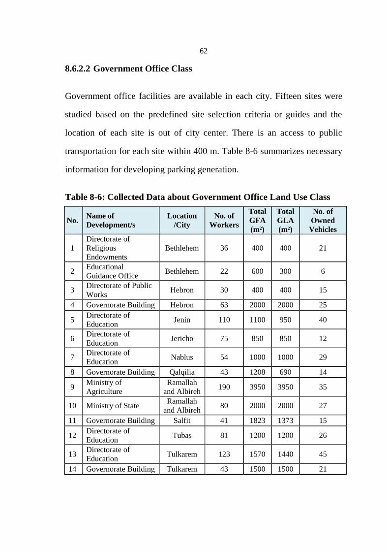
62
8.6.2.2 Government Office Class
Government office facilities are available in each city. Fifteen sites were
studied based on the predefined site selection criteria or guides and the
location of each site is out of city center. There is an access to public
transportation for each site within 400 m. Table 8-6 summarizes necessary
information for developing parking generation.
Table 8-6: Collected Data about Government Office Land Use Class
No. Name of
Development/s
Location
/City
No. of
Workers
Total
GFA
(m²)
Total
GLA
(m²)
No. of
Owned
Vehicles
1
Directorate of
Religious
Endowments
Bethlehem 36 400 400 21
2 Educational
Guidance Office Bethlehem 22 600 300 6
3 Directorate of Public
Works Hebron 30 400 400 15
4 Governorate Building Hebron 63 2000 2000 25
5 Directorate of
Education Jenin 110 1100 950 40
6 Directorate of
Education Jericho 75 850 850 12
7 Directorate of
Education Nablus 54 1000 1000 29
8 Governorate Building Qalqilia 43 1208 690 14
9 Ministry of
Agriculture
Ramallah
and Albireh 190 3950 3950 35
10 Ministry of State Ramallah
and Albireh 80 2000 2000 27
11 Governorate Building Salfit 41 1823 1373 15
12 Directorate of
Education Tubas 81 1200 1200 26
13 Directorate of
Education Tulkarem 123 1570 1440 45
14 Governorate Building Tulkarem 43 1500 1500 21

63
8.6.3 Retail Land Use
As noted in the methodology chapter, many sites were selected within the
study area that fulfills the predefined criteria. The studied sites were 17
supermarket land use class and 8 strip retail. In addition, one shopping
center was studied, which is the only one in the West Bank that complies to
the criteria. GLA, GFA, and number of workers are the main independent
variables of retail land use. Table 8-7, Table 4-8, and Table 4-9 present the
collected information of retail land use classes.
8.6.3.1 Supermarket Class
Supermarket covers almost large percent of retail. The selected sites for the
purpose of developing parking generation were selected based on being in
the peripheral area and fulfilling the predefined criteria of ITE for site
selection step. The selected sites shared high percentage of similar
characteristics and scale. Small shops were excluded, supermarket sites
without acceptable surrounding environments were also excluded, and
variations among cities were also included.
8.6.3.2 Strip Retail Class
The selection of strip retail land use class was difficult because there were
obstacles facing the researcher such as almost all strip retail are close to
urban areas and the existence of other land use types besides strip retail
leads to excluding the site. Public transportation routes serviced all sites of
this type of land use. Shopping Center Class

64
Shopping center represents the largest size market in terms of area,
diversity of available goods, etc. The only shopping center available in the
West Bank cities that complies with the site selection criteria is Plaza Mall,
in Albireh City as shown in Table 4-9. Access of public transportation is
available at this site.
Table 8-8 shows the collected information about strip retail classes in terms
of number of workers, GFA, gross leasable area (GLA), and number of
vehicles owned by workers and development.
Table 8-7: Collected Data about Supermarket Land Use Class
No. Name of
Development/s
Location/
City
No. of
Workers
Total
GFA
(m²)
Total
GLA
(m²)
No. of
Owned
Vehicles
1 Al Moghrabee
Supermarket Bethlehem 5 240 240 5
2 Khater Supermarket Bethlehem 5 200 200 3
3 Al Yazan Supermarket Hebron 5 170 170 7
4 Supermarket and
Coffee of Abu Mazin Hebron 5 520 520 2
5 Saif Side Supermarket Jenin 3 300 300 2
6 Ar Rjoub Supermarket Jericho 2 113 113 1
7 Bravo Supermarket -
Rafidia Main Str. Nablus 15 650 650 2
8 Wahet Al Makhfeya Nablus 6 320 320 2
9 Al Karmel
Supermarket Qalqilia 14 700 700 2
10 Bravo Supermarket -
Al Masyoun
Ramallah
and
Albireh
12 1000 1000 1
11 Bravo Supermarket -
Al Tyreh
Ramallah
and
Albireh
15 1200 1200 2
12
Green Land
Supermarket - Al
Tyreh
Ramallah
and
Albireh
3 300 300 1
13 Almadina
Supermarket Tubas 2 110 110 1

65
No. Name of
Development/s
Location/
City
No. of
Workers
Total
GFA
(m²)
Total
GLA
(m²)
No. of
Owned
Vehicles
14 Al Islameya
Supermarket Tulkarem 12 490 490 5
15 Dallas Supermarket Tulkarem 4 420 420 2
8.6.3.3 Shopping Center Class
Shopping center represents the largest size market in terms of area,
diversity of available goods, etc. The only shopping center available in the
West Bank cities that complies with the site selection criteria is Plaza Mall,
in Albireh City as shown in Table 4-9. Access of public transportation is
available at this site.
Table 8-8: Collected Data about Strip Retail Land Use Class
No. Name of Development/s Location/
City
No. of
Workers
Total
GFA
(m²)
Total
GLA
(m²)
No. of
Owned
Vehicles
1 Alkarkafah Strip Retail Bethlehem 9 210 210 6
2 Ras Aljora Area Strip
Retail Hebron 28 980 980 17
3 Asira Ash Shamalieh
Main Street Strip Retail Nablus 11 275 275 9
4 Ishtar Shops Strip Retail Nablus 6 200 200 4
5 Near Fehmi Gas Station
Strip Retail Qalqilia 8 196 196 6
6 Al Masyoun Strip Retail
Ramallah
and
Albireh
14 1200 1200 4
7 Near Al Quds Street Strip
Retail
Ramallah
and
Albireh
5 180 180 3
8
Near Telecommunica-
tions Company Strip
Retail - Paltel
Tulkarem 11 265 265 5

66
Table 8-9: Collected Data about Shopping Center Land Use Class
No. Name of
Development/s
Location/
City
No. of
Worke
rs
Total
GFA
(m²)
Total
GLA
(m²)
No. of Owned
Vehicles
1 Plaza Mall Albireh 37 5500 4200 20
8.7 Parking Accumulation
Two days from among the three typical weekdays (Monday, Tuesday, and
Wednesday) were used to conduct traffic survey count for each site. The
peak periods of adjacent streets of some sites coincided with the peaks of
the studied sites during AM and PM periods, and this was noticed forall
sites of office land use type. In office land use, three periods were analyzed
which are: AM, PM (which represent the peaks of the sites and adjacent
streets during morning and evening), and the peak of the development,
which represents the maximum recorded value during all periods, and this
should be used for design purposes.
Different time periods during the day are used for conducting the parking
accumulation. The difference in counting times was due to the nature of the
surveyed sites, as well as the surrounding conditions. Parking accumulation
is conducted during the following hours: 7:00-9:00 AM and 14:00-17:00
PM for residential land use, 7:00-10:45 AM and 12:00-17:00 PM for office
land use, and 7:00 AM to 21:00 PM for retail land use.

67
8.7.1 Residential Land Use
Parking accumulation of residential land use was counted manually for two
days, and two peak periods with different hours of the adjacent streets in
each day (AM and PM). Table 4-10, Table 4-11, and Table 4-12 show the
average peak parking accumulation for the two periods which represents
the average maximum peak of the two-day count (Parking Demand).
Table 8-10: Attached Housing Land Use Class Parking Accumulation
No. Name of Development/s Location/City
Parking
Demand
(AM)
Parking
Demand
(PM)
1 Doctors' Housing - Al Jabriat Jenin 17 13
2 Doctors' Housing Nablus 36 12
3 Al Ata'ot Housing Qalqilia 15 10
4 An Najmeh Housing - Abu Qash Ramallah and
Albireh 35 21
5 Education Housing Tulakrem 12 9
Table 8-11: Detached Housing Land Use Class Parking Accumulation
No. Name of Development/s Location/City
Parking
Demand
(AM)
Parking
Demand
(PM)
1 Engineers Housing - Beit
Sahour Bethlehem 40 47
2 Az Zaytona Housing Hebron 49 45
3 Al Khedawi Housing Jericho 4 6
4 Engineers Housing - Al
Makhfeya Nablus 68 45
5 Tayba Housing Nablus 12 14
6 Swaileh Villas Qalqilia 12 18
7 Al Dawha Housing - Bir Zeit Ramallah and
Albireh 48 43
8 Social Affairs Housing Tulkarem 26 12

68
Table 8-12: Apartments Housing Land Use Class Parking
Accumulation
No. Name of Development/s Location/City
Parking
Demand
(AM)
Parking
Demand
(PM)
1 Yasso' Child Housing Bethlehem 23 13
2 Al Mohtaseb Building Hebron 5 5
3 Palestinian Housing Jenin 12 13
4 Al Ajlouni Housing Jericho 3 4
5 ANNU Housing - Al Ma'jeen Nablus 26 23
6 An Noor Building Nablus 9 8
7 Old Qalqilia Housing Qalqilia 13 24
8 New Qalqilia Housing Qalqilia 24 38
9 BirZeit University Housing Ramallah and
Albireh 27 23
10 Al Jawhara Tower Tulkarem 11 9
8.7.1 Office Land Use
The same counting methods of residential land use and periods were used
for developing average maximum accumulation of parked vehicles for
office land use. Table 4-13, Table 4-14, and Table 4-15 show the outputs of
survey process. Parking demand herein and after represents the average
peak value of the two-day parking counts. Whilst, maximum parking
demand is the maximum parking demand of the development.

69
Table 8-13: General Office Class Parking Accumulation
No. Name of Development/s Location/City
Parking
Demand
(AM)
Parking
Demand
(PM)
Max.
Parking
Demand
1 Aabdeh Building - Morra
Intersection Hebron 9 8 9
2 Al Isra' Building - Faisal Str. Nablus 21 34 34
3 Jawwal Building - Rafidia
Main Str. Nablus 8 15 15
4 Ugarit Building - Near Al
Ersal Str.
Ramallah and
Albireh 16 18 18
5 Bdran Complex Tulkarem 14 13 14
Table 8-14: Institutional Office Class Parking Accumulation
No. Name of Development/s Location/City
Parking
Demand
(AM)
Parking
Demand
(PM)
Max.
Parking
Demand
1 Palestinian Insurance
Company Bethlehem 17 12 17
2 Telecommunication
Company - Paltel Jenin 21 14 21
3 Telecommunication
Company - Paltel Nablus 159 153 159
4 Al Mashriq Insurance
Company
Ramallah and
Albireh 31 48 48
5 Alwatanya Company Ramallah and
Albireh 112 127 127
6 Jawwal Company - Main
Headquarter
Ramallah and
Albireh 310 313 313
7 Telecommunication
Copmany - Paltel Tulkarem 16 11 16

70
Table 8-15: Government Office Class Parking Accumulation
No. Name of Development/s Location/City
Parking
Demand
(AM)
Parking
Demand
(PM)
Max.
Parking
Demand
1 Directorate of Education Bethlehem 8.5 8 10
2 Directorate of Religious
Endowments Bethlehem 7 6 8
3 Educational Guidance
Office Bethlehem 7 6 7
4 Directorate of Public
Works Hebron 19 17 21
5 Governorate Building Hebron 26 22.5 27
6 Directorate of Education Jenin 30.5 29 32
7 Directorate of Education Jericho 15 13.5 18
8 Directorate of Education Nablus 26.5 30 30
9 Governorate Building Nablus 15.5 19.5 21
10 Ministry of Agriculture Ramallah and
Albireh 38 33.5 40
11 Ministry of State Ramallah and
Albireh 19.5 22.5 25
12 Governorate Building Salfit 23.5 34.5 39
13 Directorate of Education Tubas 24.5 26 28
14 Directorate of Education Tulkarem 30.5 24 33
15 Governorate Building Tulkarem 22 23.5 29
8.7.2 Retail Land Use
Medium to large Supermarket, Strip, and Shopping Center Retail land use
classes were counted for two days in two peak periods to capture the
highest peak. There is no AM and PM unified parking accumulation for all
sites because the peak periods of each site are different from another.
Therefore, parking counts of two peaks were conducted in order to capture
the maximum parking demand of the facility.

71
Table 4-16, Table 4-17, and Table 4-18 show the average maximum
parking accumulation of each development during the two weekdays.
Table 8-16: Supermarket Parking Accumultation
No. Name of Development/s Location
/City
Parking
Demand
(First
Peak)
Parking
Demand
(Second
Peak)
Max.
Parking
Demand
1 Al Moghrabee Supermarket Bethlehe
m 5 5 5
2 Khater Supermarket Bethlehe
m 7 7 7
3 Al Yazan Supermarket Hebron 6 10 10
4 Plaza Supermarket - Bravo Hebron 12 10 12
5 Supermarket and Coffee of
Abu Mazin Hebron 3 8 8
6 Saif Side Supermarket Jenin 6 7 7
7 Ar Rjoub Supermarket Bethlehe
m 9 6 9
8 Bravo Supermarket -
Rafidia Main Str. Nablus 16 19 19
9 Wahet Al Makhfeya Nablus 3 4 4
10 Al Karmel Supermarket Qalqilia 8 7 8
11 Bravo Supermarket - Al
Masyoun
Ramalla
h and
Albireh
19 15 19
12 Bravo Supermarket - Al
Tyreh
Ramalla
h and
Albireh
24 23 24
13 Green Land Supermarket -
Al Tyreh
Ramalla
h and
Albireh
10 18 18
14 Max Mar Supermarket - Al
Ersal Main Str.
Ramalla
h and
Albireh
59 40 59
15 Almadina Supermarket Tubas 3 4 4
16 Al Islameya Supermarket Tulkare
m 5 7 7
17 Dallas Supermarket Tulkare
m 4 4 4

72
Table 8-17: Strip Class Parking Accumulation
No. Location of Strip Location/
City
Parking
Demand
(First
Peak)
Parking
Demand
(Second
Peak)
Max.
Parking
Demand
1 Alkarkafah Strip Retail Bethlehem 6 7 7
2 Ras Aljora Area Strip Retail Hebron 19 19 19
3 Asira Ash Shamalieh Main
Street Strip Retail Nablus 6 9 9
4 Ishtar Shops Strip Retail Nablus 6 8 8
5 Near Fehmi Gas Station
Strip Retail Qalqilia 8 7 8
6 Al Masyoun Strip Retail
Ramallah
and
Albireh
15 14 15
7 Near Al Quds Street Strip
Retail
Ramallah
and
Albireh
11 9 11
8
Near Telecommunication
Company Strip Retail -
Paltel
Tulkarem 6 7 7
Table 8-18: Shopping Center Class Parking Accumulation
No. Name of Development/s Location
/City
Parking
Demand
(First Peak)
Parking
Demand
(Second
Peak)
Max.
Parking
Demand
1 Plaza Mall
Ramallah
and
Albireh
120 124 124

73
9 Chapter Five
Data Analysis and Outputs
9.1 Introduction
This chapter analyzes collected data and provides discussion of the outputs.
Statistical tools are used to estimate parking demand for morning, evening,
and peak periods.
The following sections summarize the outputs of data analysis of each
class of land use using SPPS.
9.2 Simple Regression Analysis
Neither regression nor correlation analyses can be interpreted as estimating
cause-and-effect relationships. They can indicate only how or to what
extent variables are associated with each other. Confidence interval of 95%
is used when there are more than 20 sites available as noted by the Institute
of Transportation Engineers (ITE, 2010). Low confidence level could be
considered for small sample size such as 68% (one std. from the mean) and
95% (approximately two std. from the mean) (Smith, 1990). Higher
confidence level is recommended to ensure high percentage of reliability.

74
9.2.1 General Form of Parking Generation Models/ Equations
The collected data are analyzed using regression analysis as follow:
Simple Regression with Intercept
The following equations represent the formulas of produced parking
generation model.
P = β → Linear
P = β → Power
P = β → Exponential
P = β → Logarithmic
P: Parking Demand (Dependent Variable)
X: Independent Variable
β1: Variable Coefficient (Slope)
C: Constant (Intercept)
Note: The above equations have an estimation error (єi) as shown in
Methodology Chapter (sub-section 3.3.3)

75
9.3 Data Analysis
Linear and nonlinear regression analysis produced models, which are used
in predicting parking demand. Logarithmic, power, exponential and linear
regression models are conducted in the collected data and the best fit model
is included. These developed models have various powers of prediction;
therefore, comparison among models of same independent variable should
be based on the residuals plot, confidence level, R2, and RMSE (standard
error of the estimate) (Shacham et al., 1996). Furthermore, validation of
models and verification of models/rates are good indicators for their
accuracy in prediction.
The following subsections present the analysis of collected data associated
with the three land uses and their classes. The most appropriate form of the
model for each independent variable is provided. Other forms were
investigated; however, not presented.
Analysis of one example is presented in details (AH class), and only the
main outputs of others classes are presented in tables.
The final outputs of this chapter is summarized in Appendix (D) and
sample form is shown in Table 5-1, which contains the produced models
and rates, and their associated parameters such as average size of data,
standard deviation, confidence interval, data plot, equation, R2, residuals

76
plot, test of normality of residuals, mean, range, minimum, maximum, and
coefficient of variation (CV).
Table 9-1: Parking Generation Sheet Form
Average Peak Parking Demand vs. Number of Inhabitants
Survey Time Range
Number of Sites
Average Size
Standard Deviation
Coefficient of Variation (CV)
Range
Rate
85th
Percentile
33rd
Percentile
Model
Model Confidence Interval
Coefficient of Determination (R2)
9.3.1 Descriptive Statistics
This section represents descriptive statistics that is used to organize,
interpret, and clarify the collected data in a meaningful form. Descriptive
statistics of variables are presented in Appendix (C). These statistics should
be used for interpreting the results of analysis and ease of understanding
the data and the models such as mean, standard deviation, range, and
skewness, which is used to indicate degree of asymmetry of the probability
distribution of a random variable about its mean (MacGillivray et al.,
1988). In addition, Coefficient of Variation (CV) shows the variation of
data around the mean and measures the concentration of data. This

77
coefficient is computed by dividing the standard deviation by the mean and
it is expressed as percentage. Importance of this coefficient is to remove
the misunderstanding of variance when it has small value because this
coefficient gives percentage with respect to mean. There are no specific
limits for CV but a value of 10% could be the acceptable upper limit
(Wesrgard, 1999).
9.3.2 Residential Land Use
Parking accumulation during AM and PM peak periods of the adjacent
streets are analyzed. Indeed, some agencies or references use vehicle
ownerships as parking demand and add small percentage of 10% and 5%
for circulation and visitors, respectively (Willson, 2005).
Table 9-2 and Table 9-3, which are examples of descriptive statistics of
independent variables, they will be shown in the final outputs of parking
generation models.
Table 9-2: Descriptive Statistics for No. of Inhabitants of AH
Mean Std. Deviation CV Minimum Maximum Range
108.40 45.87 42% 59 180 121
It is obvious from Table 9-2 that the average number of inhabitants is
108.4. The maximum value in the collected data of AH is 180 inhabitants
whereas the minimum is 59 inhabitants.

78
Table 9-3: Descriptive Statistics for No. of Occupied AH Units
Mean Std. Deviation CV Minimum Maximum Range
23.8 8.17 34% 13 36 23
The average number of occupied houses is 23.8 as shown in Table 9-3. The
range of values is 23 and the CV is 34%.
Therefore, good inferences about the produced model or rate could be done
when descriptive statistics of parking demand are provided.
The following subsections summarize the process of statistical analysis of
each one of three classes of residential land use.
9.3.2.1 Regression Analysis
AH, DH, and APH classes are analyzed in this section. It is noted that
almost all selected sites have an occupancy value more than 85% as shown
previously in the data collection chapter, which consistent with the set
criteria.
Parking generation is analyzed using regression analysis, as shown below.
Regression Analysis with Intercept
Table 9-4 presents the main outputs of regression analysis, which includes
the relationship between dependent variable and single independent
variable (number of occupied houses and number of inhabitants).

79
Furthermore, it provides an indication about the power or accuracy of the
attained model in prediction.
Table 9-4: AH Land Use Class Regression Analysis Parameters
Parking Demand (AM) vs. Number of Occupied AH Units
R R2 Std. Error of the Estimate
0.644 0.414 10.209
Parking Demand (AM) vs. Number of Inhabitants
R R2 Std. Error of the Estimate
0.811 0.658 7.800
The following points are interpretation of the results of regression analysis
that were included in the summary tables.
Goodness of Fit: Coefficient of Determination R2
Assessing the accuracy of prediction is achieved by studying R2. From
Table 9-4, about 40% and 65% of variation in parking demand in the AM
period is explained by number of occupied houses and number of
inhabitants, respectively.
Significance of Model: F- Test
Table 5-5 shows Analysis of Variance (ANOVA) results, which are used to
test the significance of R and R2
using F-test. In conclusion, at 95%
confidence interval, all independent variables that were used in developing
the parking demand model in the AM period are not good predictors
because the 0.241 and 0.96 are larger than 0.05. Decreasing the confidence

80
interval will be appropriate here due to small sample size, for example,
68% is appropriate here.
Table 9-5: AH Simple Linear Regression ANOVA Table
Parking Demand (AM) vs. Number of Occupied AH Units
Sum of Squares Mean Square F Sig.
Regression 221.323 221.323 2.123 0.241
Parking Demand (AM) vs. Number of Inhabitants
Sum of Squares Mean Square F Sig.
Regression 351.471 351.471 5.777 0.096
Model Coefficient Significance (Constant): T- Test
Coefficients in Table 9-6 are used to build the model by providing the
coefficients of independent variable and the constant (β and c). herefore,
at 95% the t- test showed that H0 is correct (0.937 and 0.938>0.05) for
both models, respectively.
Table 9-6: AH Simple Linear Regression Coefficients
Parking Demand (AM) vs. Number of Occupied AH Units
Unstandardized
Coefficients
Standardized
Coefficients t Sig.
B Std. Error Beta
(Constant) 1.323 15.560 0.085 0.938
Number of Occupied
AH Units 0.911 0.625 0.644 1.457 0.241
Parking Demand (AM) vs. Number of Inhabitants
Unstandardized
Coefficients
Standardized
Coefficients t Sig.
B Std. Error Beta
(Constant) 0.849 9.854 0.086 0.937
Number of Inhabitants 0.204 0.085 0.811 2.403 0.096
From Table 9-6, the Parking Generation Model for AH class during AM
period based on number of occupied AH unit is:

81
P = ------------- (1)
P: Parking Demand (AM) (Passenger Car)
X: Number of Occupied AH Units
Figure 9.1 shows the data plot of AH land use class and the regression line
in association with the coefficient of determination.
Figure 9.1: Model Plot of Parking Demand (AM) vs. No. of Occupied Houses
Note: number of occupied attached housing units means the total number
of units in development (each one AH contains two units).

82
From Table 9-6, Parking Generation Models for the AH class during AM
period based on number of inhabitants is:
P =
P: Parking Demand (AM) (Passenger Car)
X: No. of Inhabitants
In addition, the model plot presents the relationship of parking demand
with number of inhabitants is shown in Figure 9.2.
Figure 9.2: Model Plot of Parking Demnd (AM) vs. No. of Inhabitants
Indeed, the models (1 and 2) of AH land use class do not have a good
power because the significance of intercept is not significant, since P value
for both parameters is very high (>>0.05).

83
A significant intercept (<0.05) in a model only means that there is also a
constant in the model. As a result, using intercept as zero generally
increases prediction error and hence should be avoided, if possible.
Therefore, the attained R2 for the number of occupied AH units predictor is
a small value (less than 0.5). Therefore, aborting any points will affect the
model because the sample size is small. The CV showed that the variation
in data points in the first independent variable is larger than others and this
can interpret the value of R2. In essence, the minimum acceptable value of
R2
is 0.5, and models of R2 smaller than 0.5 should not be considered and
used (ITE, 2010).
Test the Normality of Residuals
The normality of residuals is essential to ensure the accuracy of the
developed model. Figure 9.3 shows the scatter plot of the data. In this
figure, the points are close to a diagonal line; therefore, the residuals
appear to be approximately normally distributed without considering the
sample size. The deviations of points from diagonal line weaken the
produced model in prediction, and at the same time affect the strength of
model.

84
Figure 9.3: Residual Normality Plot
The summation of residuals is preferred to be zero value in order to ensure
accurate prediction of parking demand. Figure 9.4 shows that there is an
asymmetry distribution around the mean. Thus, using the model carefully
in prediction is important to avoid erroneous prediction because this
deviation weakens the model in prediction.

85
Figure 9.4: Distribution of Residuals around Mean
Confidence Interval Bounds
Table 9-7 presents some statistics values of the t-Student distribution.
These values are used in calculating the confidence interval. Lower and
upper bounds, which form the range of predictions (rates), can be
computed using the following formulas:
=

86
Z: Based on number of degree of freedom (df) = N-1 (N: sample Size).T-
Distribution is used in the analysis.
Table 9-7: Critical Values of the t - Distribution (Z)
df` Confidence Level (%)
90 95 99
2 2.920 4.303 9.925
3 2.353 3.182 5.841
4 2.132 2.776 4.604
5 2.015 2.571 4.032
8 1.943 2.306 3.355
10 1.812 2.228 3.169
15 1.753 2.086 2.845
20 1.725 2.009 2.678
Source: (Montgomery et al., 2002)
Table 9-7 is used to compute confidence interval bounds for every model.
Parking generation models of AH Residential Land Use class are shown in
Table 9-8 and Table 9-9. These tables present the models and rates with
their associated statistics during the AM and PM periods.

87
Table 9-8: Parking Generation Models for AH Residential Land Use Class in AM and PM Periods
No. Period Regression Model Type R2
R2
adj.
F-test MS
t- test Std. Error of
the Estimate
Independent
Variable F Sig. t Sig.
1
AM
P= 0.911*X+ 1.323 Linear 0.41 0.22 2.12 0.241 104 0.085 0.938 10.2
Number of
Occupied AH
Units
2 P= 0.204*X+ 0.849 Linear 0.66 0.54 5.78 0.096 61 0.086 0.937 7.8 Number of
Inhabitants
3
PM
P= 2.66 * X 0.516
Power 0.28 0.04 1.159 0.361 0.12 0.651 0.561 0.35
Number of
Occupied AH
Units
4 P= 0.708 * X 0.635
Power 0.56 0.41 3.83 0.145 0.07 -0.229 0.833 0.27 Number of
Inhabitants

88
Table 9-9: Parking Generation Rates for AH Residential Land Use
Class in AM and PM Periods
No. Period Rate Std.
Deviation CV (%) Range
1 AM
0.95 space per occupied AH unit 0.39 41 1.02
2 0.21 space per inhabitant 0.07 32 0.16
3 PM
0.55 space per occupied AH unit 0.25 45 0.58
4 0.12 space per inhabitant 0.05 39 0.12
The produced models' forms of AH class for both AM and PM periods
were linear and power, respectively.
Table 9-8 shows that all regression models are not significant at 95%
confidence interval.
From Table 9-8, the produced models for PM period and the first model in
AM period are not strong models for prediction, because they have low
values of R2. Therefore, it is preferable to use the rates in Table 9-9.Std.
Error of the Estimate also gives an indication about the concentration of the
data around the fitted equation. Values of 10.2 and 7.8 are the RMSE of the
linear regression model based on the predictive variables number of
occupied houses and number of inhabitants, respectively. On the other
hand, 0.35 and 0.27 are the RMSE of the power regression models based
on the number of occupied houses and number of inhabitants, respectively.
Therefore, the best fit model means highest R2 and lowest RMSE.

89
Therefore, the small sample size affected the strength of all produced
models either rates or models. Rates are recommended to use for AH land
use class because the produced models are poor.
In essence, prediction points should be within the plot area in order to get
the level of accuracy for the used model. Extrapolation should be used
carefully especially when the model is week in prediction to ensure
minimal error. Confidence level could affect the use of produced models;
for example at confidence interval 90%, the produced model of R20.66 is
recommended to use.
DH and APH Land Use classes are similarly analyzed. As in the previous
analysis of AH class, different types of transformation (linear, logarithmic,
exponential, and power) are checked, and only models that have the best fit
are recorded.
Table 9-10 and Table 9-11 summarize the results of regression analysis for
DH land use class. These tables include parking generation models and
rates for both AM and PM periods.

90
Table 9-10: Parking Generation Models for DH Residential Land Use Class in AM and PM Periods
No. Period Regression Model Type R2
R2
adj.
F-test
MS
t-test
RMSE Independent Variable
F Sig. t Sig
1
AM
P= 0.914*X 0.911
Power 0.82 0.79 26.92 0.002 0.2 -0.14 0.894 0.448 Number of Occupied DH Units
2 P= 0.157* X 1.065
Power 0.91 0.90 61.06 0 0.1 -2.89 0.029 0.314 Number of Inhabitants
3
PM
P= 14.951*ln (x)-20.34 Log* 0.55 0.48 7.38 0.035 167 -1.09 0.315 12.918 Number of Occupied DH Units
4 P= 16.781*ln (x)-50.38 Log* 0.67 0.62 12.20 0.013 123 -2.19 0.07 11.075 Number of Inhabitants
* log: Logarithmic

91
Table 9-11: Parking Generation Rates for DH Residential Land Use
Class in AM and PM Periods
No. Period Rate Std.
Deviation
CV
(%) Range
1 AM
0.93 space per occupied DH unit 0.40 43 0.94
2 0.22 space per inhabitant 0.06 29 0.16
3 PM
0.82 space per occupied DH unit 0.56 69 1.93
4 0.20 space per inhabitant 0.11 57 0.16
In Table 9-10, the produced models in AM period are good estimators for
parking generation; because they produced good values of R2, RMSE,
confidence level, and residuals plot. Furthermore, the produced models for
AM period are significant at 95% confidence interval. Thus, these models
are recommended to be used in prediction.
In the PM period, the developed models in Table 9-10 are fair to good in
prediction with respect to the associated statistical parameters of each
model. Therefore, using rates included in Table 9-11are recommended, but
the model which used the number of inhabitants as independent variable
could be used because it has an acceptable R2.
Independent variable should be within the range of data when using rates
and models to ensure good level of accuracy.
Table 9-12 and Table 9-13 summarize the results of regression analysis for
APH land use class for both AM and PM periods.

92
Logarithmic models are the best fit models in AM period whereas power
and exponential models are the best fit models of PM period. From the
results in Table 9-12, it is not recommended to use any model in both AM
and PM periods, because the produced regression models are poor models
in prediction based on the attained R2, F-test, and other supporting
statistical parameters. Therefore, using the produced rates included in
Table 9-13 instead of models is recommended.

93
Table 9-12: Parking Generation Models for APH Residential Land Use Class on AM and PM Periods
No. Period Regression Model Type R2
R2
adj.
F-test
MS
t-test Std.
Error
of the
Estim
ate
Independent
Variable F Sig. t Sig.
1
AM
P= 11.379*ln(x)-40.97 Log 0.44 0.37 6.38 0.035 53 -1.8 0.11 7.3 Number of
Inhabitants
2 P= 11.035*ln(x)-76.032 Log 0.36 0.28 4.54 0.066 61 -1.75 0.118 7.8 GFA (sq. m.)
3 P= 12.534*ln(x)-25.925 Log 0.39 0.31 5.11 0.054 58 -1.38 0.206 7.6
Number of
Occupied
Dwelling Units
(DU's).
4
PM
P= e 1.816*X
Exp* 0.28 0.18 3.03 0.12 0.5
0 3.93 0.004 0.703
Number of
Inhabitants
5 P= 0.025*X 0.741
Power 0.23 0.13 2.37 0.162 0.5
3 -0.91 0.388 0.725 GFA (sq. m.)
6 P= 0.424*X+ 2.278 Linear 0.38 0.30 4.89 0.058 81 0.34 0.745 9 Number of
Occupied DU's.
*Exp: Exponential

94
Table 9-13: Parking Generation Rates for APH Residential Land Use
Class on AM and PM Periods
No. Period Rate Std.
Deviation CV (%) Range
1
AM
0.09 space per Inhabitant 0.06 66 0.20
2 0.33 space per 100 sq. m. of GFA 0.22 65 0.71
3 0.51 space per occupied DU 0.30 59 0.82
4
PM
0.09 space per Inhabitant 0.10 106 0.31
5 0.33 space per 100 sq. m. of GFA 0.28 87 0.91
6 0.49 space per occupied DU 0.45 92 1.57
9.3.2.2 The Best Models and Rates for Residential Land Use
Table 9-14 summarizes the produced models (R2>0.6) or rates for each
class based on number of inhabitants and occupied units, while
Table 9-15 summarizes the applicable and recommended models and rates
of parking generation during AM and PM periods of residential land use
for the most appropriate independent variable.
The recommended models/rates are the most powerful ones among others
based on statistical parameters (R2>0.6) and the predominant used
independent variable, as applicable.

95
Table 9-14: Parking Generation Models/Rates of Resdential Land Use
Class Period Independent Variable Model R2 Rate
AH
AM Number of Occupied AH Units - - 0.95 space per Occupied AH unit
Number of Inhabitants P= 0.204*X+ 0.849 0.66 -
PM No. of Occupied AH units - - 0.55 space per Occupied AH unit
Number of Inhabitants - - 0.12 space per inhabitant
DH
AM Number of Occupied DH Units P= 0.914*X
0.911 0.82 -
Number of Inhabitants P= 0.157* X 1.065
0.91 -
PM Number of Occupied DH Units - - 0.82 space per Occupied AH unit
Number of Inhabitants P= 16.781*ln(x)-50.38 0.67 -
APH
AM
Number of Inhabitants - - 0.09 space per inhabitant
GFA (100 sq. m.) - - 0.33 space per 100 GFA
Number of Occupied DU's. - - 0.51 space per Occupied DU
PM
Number of Inhabitants - - 0.09 space per inhabitant
GFA (sq. m.) - - 0.33 space per 100 GFA
Number of Occupied DU's. - - 0.49 space per Occupied DU

96
Table 9-15: Recommended Parking Generation Models/Rates of Resdential Land Use
Class Period Independent Variable Model R2 Rate Recommended
AH
AM Number of Inhabitants P= 0.204*X+ 0.849 0.66 0.21 space per inhabitant Model
PM Number of Inhabitants P= 0.708 * X 0.635
0.56 0.12 space per inhabitant Rate
DH
AM Number of Inhabitants P= 0.157* X 1.065
0.91 0.22 space per inhabitant Model
PM Number of Inhabitants P= 16.781*ln(x)-50.38 0.67 0.20 space per inhabitant Model
APH
AM Number of Occupied DU's. P= 12.534*ln(x)-25.925 0.39 0.51 space per Occupied DU Rate
PM Number of Occupied DU's. P= 0.424*X+ 2.278 0.38 0.49 space per Occupied DU Rate

97
Do the developed parking generation models/rates from this study differ
from Palestinian regulations? Appendix F presents the needed parking
spaces for residential land use regardless of its classes and surrounding
environment. One space per dwelling units shall be provided, according to
local regulations (Appendix F). However the produced models/rates in this
study provide different values for land use type (0.51-0.95 space per DU),
and these values depend on a class of residential land use.
Moreover, a comparison of the recommended models/rates of this research
with the common international parking generation (ITE) is shown in Table
9-16.
Table 9-16: The Obtained Parking Generation Models/Rates of
Residential Land Use vs.ITEModels/Rates *
Land use
class Period
Result of Recommended
Model/Rate ITE Model/Rate Result
AH AM 0.30 space per Occupied DU 1.73 space per Occupied DU
DH PM 0.30 space per Occupied DU 0.35 space per Occupied DU
APH AM 0.51 space per Occupied DU 1.23 space per Occupied DU
PM 0.49 space per Occupied DU 1.2 space per Occupied DU
*Source: (ITE, 2010)
The differences shown in Table 5-16 justify using local studies rather than
international studies. Abu Dhabi regional study has detailed rates for many
land use types and is not appropriate for similar comparison.

98
9.3.3 Office Land Use
Office Land uses are classified into three classes based on the local
condition Chapter Four. General, Institutional, and Government Office
Land use classes are analyzed in the following subsections to find models
or rates of predicting parking demand. Three peaks were used in analysis:
AM and PM peaks of the adjacent streets as well as the maximum peak
period of development.
Table 9-17 and Table 9-18 show that the parking generation models based
on the peak parking of development. These tables involve different forms
of regression; exponential, linear, and power for General Office class.
Linear regression models are the best fit for Institutional Office class. On
the other hand, Government Office class has two types of regression model
forms, which are logarithmic and power models.
As shown in Table 9-17, the produced models of General Office class
based on GFA, GLA, and number of workers' vehicles are the best models,
because they have high R2, and they are significant at 95% confidence
level. Therefore, using these three models in prediction is recommended,
while, the number of workers as an independent variable for parking
generation rate shown in Table 9-18 should be used instead of poor model
(R2<0.6) in Table 9-17.

99
Table 9-17: Parking Generation Models for Office Land Use Classes Based in Peak Parking of Development
No. Land Use
Class Regression Model Type R
2
R
adj.
F-test MS
t-test RMSE Independent Variable
F Sig. t Sig.
1
General
Office
P= 20.88*e-0.008x
Exp 0.03 0 0.082 0.793 0.30 3.11 0.053 0.547 Number of Workers
2 P= 27502*X-1.072
Power 0.93 0.91 40.72 0.008 0.02 8.74 0.003 0.145 GFA (sq. m.)
3 P=-17.62*ln(x) +
137.32 Log 0.88 0.83 21.11 0.019 15 5.26 0.013 3.892 GLA (sq. m.)
4 P= -28.51*ln(x) + 96.07 Log 0.78 0.71 10.71 0.047 27 3.98 0.028 5.162 Number of Workers'
Vehicles
1
Institutional
Office
P= 0.48*X-0.57 Linear 0.97 0.97 182.17 0.000 387 -0.05 0.959 19.677 Number of Workers
2 P= 0.025*X-2.18 Linear 0.97 0.97 170.25 0.000 414 -0.20 0.850 20.335 GFA (sq. m.)
3 P= 0.024*X+ 3.26 Linear 0.95 0.94 98.04 0.000 703 0.23 0.825 26.519 GLA (sq. m.)
4 P= 1.03*X-7.17 Linear 0.95 0.94 102.62 0.000 673 -0.49 0.640 25.949 Number of Workers'
Vehicles
1
Government
Office
P 10.79*ln(x)-20.99 Log 0.46 0.42 10.38 0.007 51 -1.49 0.163 7.196 Number of Workers
2 P 11.38 ln(x)-56.91 Log 0.61 0.57 18.43 0.001 38 -3.03 0.010 6.171 GFA (sq. m.)
3 P 10.62*ln(x)-49.92 Log 0.64 0.61 21.15 0.001 35 -3.10 0.009 5.912 GLA (sq. m.)
4 P= 2.8*X 0.664
Power 0.45 0.38 9.11 0.008 0.17 0.79 0.140 0.418 Number of Workers'
Vehicles

100
Table 9-18: Parking Generation Rates for Office Land Use Classes
Based in Peak Parking of Development
No.
Land
Use
Class
Rate Std.
Deviation
CV
(%) Range
1
General
Office
P= 0.52 space per worker 0.31 59 0.77
2 P= 1.57 space per 100 sq. m. of GFA 2.34 150 5.78
3 P= 1.81 space per 100 sq. m. of GLA 3.46 192 8.21
4 P= 1.09 space per worker vehicle 1.19 110 3
5 Institutio
nal
Office
P= 0.48 space per worker 0.38 79 1.04
6 P= 2.41 space per 100 sq. m. of GFA 1.82 75 5.28
7 P= 2.50 space per 100 sq. m. of GLA 1.81 73 5.28
8 P= 0.96 space per worker vehicle 0.49 51 1.46
9 Governm
ent
Office
P= 0.33 space per worker 0.19 58 0.65
10 P= 1.68 space per 100 sq. m. of GFA 0.01 59 3.79
11 P= 1.82 space per 100 sq. m. of GLA 0.01 55 3.79
12 P= 1.17 space per worker vehicle 0.61 52 2.57
Furthermore, Institutional Office class has strong models and rates as
shown in Table 9-17 and Table 9-18. Thus, using either models or rates in
prediction is applicable, but models are recommended to be used because
they are preferred statistically. Coefficient of Variation is high enough to
conclude that the data has high variance, and this means the distribution of
data does not follow the normal distribution (test of normality).
Government Office land use class showed fair and poor parking generation
models as shown in Table 9-17. The produced models that used GFA and
GLA as independent variables could be used because they produced
acceptable R2 (> 60%). As a result, the produced rates in Table 9-18 for
Government Office class are recommended to use instead of models,
especially for number of workers and number of workers vehicles
independent variables.

101
Table 9-19 and Table 9-20 show the developed models and rates of office
land use for the peak of adjacent streets during the AM period.
As shown in Table 9-19, General Office class produced poor parking
generation models. In addition, Institutional Office class models or rates
are strong predictor at high level of confidence. As aforementioned, the
models are better than rates. Thus, Institutional Office models presented in
Table 9-19 are recommended to use.
Finally, Government Office class produced fair to good models as shown
in Table 9-19. Therefore, using the statistically good models is
recommended.
The peak parking accumulation during the PM was also studied as shown
in Table 9-21 and Table 9-22.

102
Table 9-19: Parking Generation Models for Office Land Use Classes Based in AM Peak Accumulation
No.
Land
Use
Class
Regression Model Type R2
R
adj.
F-test
MS
t-test
RMSE Independent
Variable F Sig. t Sig.
1
General
Office
33.148*e-0.029x
Exp 0.44 0.25 2.33 0.224 0.14 5.26 0.013 0.3736 Number of
Workers
2 P -9.49 ln(x)+79.32 Log 0.55 0.40 3.61 0.154 19 2.28 0.107 4.320 GFA (sq. m.)
3 P -7.27 ln(x)+62.66 Log 0.44 0.25 2.36 0.222 23 1.95 0.147 4.794 GLA (sq. m.)
4 P= -11.29*ln(x)+ 44.37 Log 0.36 0.15 1.71 0.283 26.2 1.86 0.160 5.118 Number of
Workers' Vehicles
1
Institutio
nal
Office
P= 0.478* X-5.269 Linear 0.97 0.96 136.16 0.000 514 -0.434 0.682 22.676 Number of
Workers
2 P= 0.025* X-7.082 Linear 0.97 0.96 144.86 0.000 484 -0.59 0.577 22.008 GFA (sq. m.)
3 P= 0.024* X-1.882 Linear 0.95 0.94 98.08 0.000 27 -0.134 0.898 26.536 GLA (sq. m.)
4 P= 15.502*e 0.012x
Exp 0.98 0.98 265.28 0.000 0.03 27.31 0.00 0.1804 Number of
Workers' Vehicles
1
Governm
ent
Office
P 11.89*ln(x)-26.93 Log 0.65 0.62 21.79 0.001 30 -2.56 0.025 5.442 Number of
Workers
2 P 10.15*ln(x)-49.96 Log 0.54 0.51 14.32 0.003 38 -2.63 0.022 6.167 GFA (sq. m.)
3 P 9.88*ln(x)-46.77 Log 0.64 0.61 21.30 0.001 30 -3.14 0.009 5.482 GLA (sq. m.)
4 P= -0.312*X+ 23.903 Linear 0.78 0.61 18.91 0.001 32 1.94 0.077 5.691 Number of
Workers' Vehicles

103
Table 9-20: Parking Generation Rates for Office Land Use Classes
Based on AM Peak Accumulation
No.
Land
Use
Class
Rate Std.
Deviation
CV
(%) Range
1
Genera
l
Office
P= 0.39 space per worker 0.23 60 0.47
2 P= 1.18 space per 100 sq. m. of
GFA 1.37 116 3.38
3 P= 1.37 space per 100 sq. m. of
GLA 2.04 149 4.79
4 P= 0.82 space per worker vehicle 0.68 0.83 1.70
5
Institut
ional
Office
P= 0.45 space per worker 0.40 88 1.10
6 P= 2.29 space per 100 sq. m. of
GFA 1.88 82 5.81
7 P= 2.37 space per 100 sq. m. of
GLA 1.87 79 5.81
8 P= 0.91 space per worker vehicle 0.53 58 1.56
9
Govern
ment
Office
P= 0.31 space per worker 0.15 48 0.44
10 P= 1.55 space per 100 sq. m. of
GFA 1.00 65 3.79
11 P= 1.69 space per 100 sq. m. of
GLA 0.99 58 3.79
12 P= 0.92 space per worker vehicle 0.30 33 1.23

104
Table 9-21: Parking Generation Models for Office Land Use Classes Based on PM Peak Accumulation
No. Land Use
Class Regression Model Type R
2
R
adj.
F-test MS
t-test RMSE
Independent
Variable F Sig. t Sig.
1
General
Office
P= 21.78*e -0.010x
Exp 0.04 0 0.133 0.759 0.36 2.88 0.063 0.60 Number of Workers
2 P= 61945*X-1.193
Power 0.95 0.93 57.34 0.005 0.02 10.05 0.002 0.136 GFA (sq. m.)
3 P= -18.4*ln(x)+142.28 Log 0.88 0.84 21.88 0.018 15.9 5.31 0.013 3.991 GLA (sq. m.)
4 P= -28.06* +94.51 Log 0.70 0.60 6.90 0.079 40 3.20 0.049 8.328 Number of Workers'
Vehicles
5
Institutional
Office
P=0.486* X-5.449 Linear 0.97 0.97 173.10 0.000 418 -0.50 0.640 20.448 Number of Workers
6 P=0.025* X-7.057 Linear 0.97 0.96 159.44 0.000 453 -0.61 0.566 21.280 GFA (sq. m.)
7 P=0.024* X-1.449 Linear 0.95 0.94 91.05 0.000 775 -0.10 0.925 27.844 GLA (sq. m.)
8 P=1.045* X-12.121 Linear 0.95 0.94 98.93 0.000 716 -0.81 0.453 26.768 Number of Workers'
Vehicles
9
Government
Office
P= 1.86*X 0.574
Power 0.37 0.32 6.98 0.022 0.22 0.69 0.502 0.465 Number of Workers
10 P= 10.47*ln(x)-51.99 Log 0.56 0.52 15.08 0.002 38 -2.72 0.019 6.196 GFA (sq. m.)
11 P= 0.289*X 0.608
Power 0.59 0.56 17.42 0.001 0.14 -1.23 0.244 0.373 GLA (sq. m.)
12 P= 2.63*X 0.659
Power 0.40 0.35 8.02 0.015 0.21 1.35 0.204 0.452 Number of Workers'
Vehicles

105
Table 9-22: Parking Generation Rates for Office Land Use Classes
Based on PM Peak Accumulation
No. Land Use
Class Rate
Std.
Deviation
CV
(%) Range
1
General
Office
P= 0.51 space per worker 0.31 61 0.78
2 P= 1.54 space per 100 sq. m.
of GFA 2.36 153 5.81
3 P= 1.78 space per 100 sq. m.
of GLA 3.48 196 8.26
4 P= 1.07 space per worker
vehicle 1.20 112 3.02
5
Institution
al Office
P= 0.46 space per worker 0.22 48 0.70
6 P= 2.33 space per 100 sq. m.
of GFA 1.20 51 3.38
7 P= 2.41 space per 100 sq. m.
of GLA 1.26 52 3.2
8 P= 0.93 space per worker
vehicle 0.32 34 0.98
9
Governme
nt Office
P= 0.31 space per worker 0.20 64 0.67
10 P= 1.57 space per 100 sq. m.
of GFA 0.01 59 3.40
11 P= 1.70 space per 100 sq. m.
of GLA 0.01 55 3.40
12 P= 0.93 space per worker
vehicle 0.46 49 2.01
As shown in Table 9-21, number of workers independent variable of
General Office class shall not be used in prediction because the analysis
showed there is a weak relationship between dependent and independent
variables. On the other hand, GFA and GLA at 95% confidence level
independent variables are good models in prediction based on the F-test.
On the other hand, the model that used number of workers vehicles as
repressor is good model at 90% confidence level based on the F-test. Thus,
using rates that were included in Table 9-22 are recommended for number
of workers and number of workers vehicles repressors.
106
The analysis of Institutional Office class produced good prediction models
and rates as shown in Table 9-21 and Table 9-22. Parking generation
models in Table 9-21 are better than rates included in Table 9-22, and this
was justified statistically.
The developed parking generation models for Government Office class in
Table 9-21 are poor models. Rates that are presented in Table 9-22 are
recommended in prediction of parking demand for Government Office.
9.3.3.1 The Best Models and Rates for Office Land Use
Table 9-23 and Table 9-24 summarize the applicable and recommended
models (R2>0.6) and rates of parking generation during periods of AM,
PM, and peak of development of office land use.
Appendix F presents the required parking spaces for office land use based
on the Palestinian MoLG regulations regardless of its classes. One space
per 70 sq. m. shall be provided according to local regulations. However,
the produced models/rates in this study provide higher values. The
developed models/rates provide different values for three classes of office
land use, while MoLG regulations provide one value for all office types.
Comparison with the ITE parking generation provides large differences.
For example, this study produces 1.5 spaces per 100 sq. m. GFA for
general office class, while the ITE provides 2.74 spaces per 100 sq. m.
GFA for office building land use. Again, this large difference justifies
using local parking generation.

107
Table 9-23: Parking Generation Models/Rates of Office Land Use
Class Period Independent Variable Model R2 Rate
Peak
GFA (sq. m.) P= 27502*X-1.072
0.93 -
GLA (sq. m.) P -17.62 ln(x)+137.32 0.88 -
Number of Workers' Vehicles P -28.51 ln(x)+96.07 0.78 -
AM
GFA (sq. m.) - - 1.18 space per 100 sq. m. GFA
GLA (sq. m.) - - 1.37 space per 100 sq. m. GLA
Number of Workers' Vehicles - - 0.82 space per worker's vehicle
PM
GFA (sq. m.) P= 61945*X-1.193
0.98 -
GLA (sq. m.) P -18.40 ln(x)+142.28 0.88 -
Number of Workers' Vehicles P -28.06 ln(x)+94.51 0.70 -
Institutional
Office
Peak
Number of Workers P= 0.48*X-0.57 0.97 -
GFA (sq. m.) P= 0.025*X-2.18 0.97 -
GLA (sq. m.) P= 0.024*X+ 3.26 0.95 -
Number of Workers' Vehicles P= 1.03*X-7.17 0.95 -
AM
Number of Workers P= 0.478* X1-5.269 0.97 -
GFA (sq. m.) P= 0.025* X-7.082 0.97 -
GLA (sq. m.) P= 0.024* X-1.882 0.95 -
Number of Workers' Vehicles P= 15.502*e 0.012x
0.98 -
PM
Number of Workers P=0.486* X-5.449 0.97 -
GFA (sq. m.) P=0.025* X-7.057 0.97 -
GLA (sq. m.) P=0.024* X-1.449 0.95 -
Number of Workers' Vehicles P=1.045* X-12.121 0.95 -
Government
Office
Peak
Number of Workers - - 0.33 space per worker
GFA (sq. m.) P 11.53*ln(x)-57.71 0.61 -
GLA (sq. m.) P 10.62*ln(x)-49.92 0.64 -
Number of Workers' Vehicles - - 1.17 space per worker's vehicle

108
Class Period Independent Variable Model R2 Rate
AM
Number of Workers P 11.89 ln(x)-26.93 0.65 -
GFA (sq. m.) - - 1.55 space per 100 sq. m. GFA
GLA (sq. m.) P 9.88*ln(x)-46.77 0.64 1.69 space per 100 sq. m. GLA
Number of Workers' Vehicles P= -0.312*X1+ 23.903 0.78 0.92 space per worker's vehicle
PM
Number of Workers - - 0.31 space per worker
GFA (sq. m.) - - 1.57 space per 100 sq. m. GFA
GLA (sq. m.) - - 1.70 space per 100 sq. m. GLA
Number of Workers' Vehicles - - 0.93 space per worker's vehicle
Table 9-24: Recommended Parking Generation Models/Rates of Office Land Use
Class Period Independent
Variable Model R
2 Rate
Recommended
General Office
Peak GFA (sq. m.) P= 27502*X-1.072
0.93 P= 1.57 space per 100 sq. m. of GFA Model
AM GFA (sq. m.) P -9.49*ln(x)+79.32 0.55 1.18 space per 100 sq. m. GFA Rate
PM GFA (sq. m.) P= 61945*X-1.193
0.98 P= 1.54 space per 100 sq. m. of GFA Model
Institutional
Office
Peak GFA (sq. m.) P= 0.025*X-2.18 0.97 P= 2.41 space per 100 sq. m. of GFA Model
AM GFA (sq. m.) P= 0.025* X-7.082 0.97 P= 2.29 space per 100 sq. m. of GFA Model
PM GFA (sq. m.) P=0.025* X-7.057 0.97 P= 2.33 space per 100 sq. m. of GFA Model
Government
Office
Peak GLA (sq. m.) P 10.62 ln(x)-49.92 0.64 1.82 space per 100 sq. m. GLA Model
AM GLA (sq. m.) P 9.88 ln(x)-46.77 0.64 1.69 space per 100 sq. m. GLA Model
PM GLA (sq. m.) P= 0.289*X 0.608
0.59 1.70 space per 100 sq. m. GLA Rate

109
9.3.4 Retail Land Use
Supermarket, Strip, and Shopping Center Retail Land use classes were
analyzed.
The analysis of the collected data regarding retail land use showed there
are two peak periods (not necessary AM or PM) of parking demand. For
example, supermarket development has two peak periods from 14:00 to
16:00 and 19:00 to 21:00, so the two peaks are in PM periods. Only the
maximum peak value for each development was analyzed, because it
represents the maximum parking demand of each development.
Data collection indicated that the GFA and GLA independent variables are
the same in Strip and Supermarket Retail classes. Therefore, only one of
them was used in the analysis, which is GLA.
Table 9-25 and Table 9-26 are summary tables of the regression analysis of
retail land use type.
Table 9-25 shows poor models for supermarket retail class, and fair to
good models for strip retail class. The produced models of supermarket
class provide low level of accuracy in prediction. Therefore, using rates
included in Table 9-26 is preferable. Whereas, the developed rates of strip
class should be used except the derived model from number of workers'
vehicles independent variable.

110
Table 9-25: Parking Generation Models for Retail Land Use Classes Based on Peak Demand of Development
No. Land Use
Class Regression Model Type R
2
R
adj.
F-test MS
t-test RMSE
Independent
Variable F Sig. t Sig.
1
Supermarket
Retail
P= 0.773*X+ 4.636 Linear 0.34 0.287 6.34 0.023 30 1.80 0.096 5.482 Number of
Workers
2 P= 0.014*X+ 3.74 Linear 0.51 0.471 13.47 0.003 22 1.75 0.104 4.722 GLA (sq. m.)
3 P= -2.947*ln(x)+ 12.384 Log 0.08 0.007 1.10 0.313 42 4.64 0.000 6.471
Number of
Workers'
Vehicles
4
Strip Retail
P= 0.492*X+ 4.843 Linear 0.68 0.625 12.65 0.012 7 2.62 0.040 2.661 Number of
Workers
5 P= 0.009*X+ 6.453 Linear 0.75 0.711 18.23 0.005 5 5.14 0.002 2.334 GLA (sq. m.)
6 P= 0.606*X+ 6.408 Linear 0.40 0.300 3.99 0.093 13 2.65 0.038 3.634
Number of
Workers'
Vehicles

111
Table 9-26: Parking Generation Rates for Retail Land Use Classes
Based on Peak Demand of Development
No. Land Use
Class Rate
Std.
Deviation
CV
(%) Range
1
Supermarket
Retail
P= 1.15 space per worker 1.05 92 3.83
2 P= 2.08 space per 100 sq. m.
of GLA 1.74 83 5.17
3 P= 3.91 space per worker
vehicle 5.93 1.52 17.60
5
Strip Retail
P= 0.82 space per worker 0.51 63 1.60
7 P= 2.22 space per 100 sq. m.
of GLA 1.13 51 3.56
8 P= 1.52 space per worker
vehicle 1.08 71 2.63
Shopping Center class was studied. Only one site is available in the study
area that has the characteristics of shopping center land use class as noted
before. Therefore, the rate is applicable to use in predicting parking
generation (see Table 9-27).
Table 9-27: Parking Generation Rates for Shopping Center Land Use
Class
Period Max. Average Parking Peak Demand
Total GFA (per 100 sq. m.) 2.25
Total GLA (per 100 sq. m.) 2.94
9.3.4.1 The Best Models and Rates for Retail Land Use
Table 9-28 and Table 9-29 summarize the applicable and recommended
models (R2>0.6) and rates of parking generation during AM and PM
periods of Retail land use.

112
Table 9-28: Parking Generation Models/Rates of Retail Land Use
Class Independent
Variable (X) Model R
2 Rate
Supermarket
Retail
Number of
Workers - -
1.15 space per
worker
GFA (100 sq. m.) - - 2.08 space per
100 sq. m. GFA
Number of
Workers Vehicle - -
3.91 space per
worker's
vehicle
Strip Retail
Number of
Workers P= 0.492*X+ 4.843 0.68
0.82 space per
worker
GFA (sq. m.) P= 0.009*X+ 6.453 0.75 2.22 space per
100 sq. m. GFA
Number of
Workers Vehicle - -
1.52 space per
worker's
vehicle
Table 9-29: Recommended Parking Generation Models/Rates of Retail
Land Use
Class Independent
Variable (X) Model R
2 Rate
Recommended
Supermarket
Retail
GFA (100
sq. m.)
P= 0.014*X+
3.74 0.51
2.08 space
per 100 sq.
m. GFA
Rate
Strip Retail GFA (sq. m.) P= 0.009*X+
6.453 0.75
2.22 space
per 100 sq.
m. GFA
Model
One space per 50 sq. m. shall be provided according to Palestinian MOLG
regulations (Appendix F).However, the produced models/rates in this study
provide higher values for parking generations such a land use type. The
developed models/rates provide different values for three classes of retail
land use, while the local regulations provide one value for all retail land
use types.

113
9.4 Models Verification and Validation
Residual plots presented in Appendix (E) show the difference between
regression lines and field measurement. All resulted models have points
that deviate from regression lines. These deviations vary from one model to
another. Therefore, as the points are close to the regression line the model
is better.
Validation and verification are used to test the ability of developed
models/equations in prediction. Indeed, the small simple size of some
classes weakens the validation and verification accuracy.
Model Validation
The validation of developed models are studied based on some statistical
parameters that are used to test the power of model such as R2 and residual
plots as shown in the aforementioned tables for each land use type, and in
Appendix (E). Validation is used to test the quality of used methodology in
producing models/equations.
Model/Rate Verification
Verification of the attained models and rates are checked based on random
samples; this sample was selected for studied land use classes to estimate
the parking demand, and make inferences about the differences between
the observations and the model estimation. If the estimated values from
models coincide or close to the observed values, the models can be

114
considered verified. For the purpose of this research and according to the
studied sample sizes, 25% of difference is acceptable as an average.
Table 9-30 shows that not all the models are verified in DH class,
particularly in the PM period. Other new sites are required to test the model
verified and make inferences.
Table 9-30: Models Verification of DH Class
Per
iod
Ind
epen
den
t V
ari
ab
le
Mo
del
Sam
ple
No.
Mo
del
Ob
serv
ed
Dif
feren
ce
AM
Number of
Occupied DH Units P= 0.911 *X
0.911
1 29 35 -17%
2 33 37 -11%
Number of
Inhabitants P=0.157* X
1.065
1 34 35 -3%
2 40 37 8%
PM Number of
Inhabitants P= 16.781* -502.77
1 35 47 -26%
2 37 36 3%
Only Government office land use class is verified among the three classes
of office land use because the sample size is large enough. The other two
classes are not verified here because the sample size of each is small.
Table 9-31 presents the estimated parking demand from previous models
(regression with intercept) for government office classes during three count
periods and the observed values.
It is obvious from Table 9-31 that almost all the developed models have
low differences (<25%).

115
Table 9-31: Models Verification of Government Office Class
Per
iod
Ind
epen
den
t
Vari
ab
le
Mod
el
Sam
ple
No.
Mod
el
Ob
serv
ed
Dif
feren
ce
Peak
GFA (sq. m.) P 11.53*ln(x)-57.71
1 19 18 6%
2 37 45 -18%
3 6 6 0%
GLA (sq. m.) P 10.62*ln(x)-49.92 1 21 18 17%
2 38 45 -16%
AM
Number of Workers P 11.89*ln(x)-26.93 1 19 18 6%
2 35 45 -22%
GLA (sq. m.) P 9.88*ln(x)-46.77 1 19 18 6%
2 35 45 -22%
Number of Workers
Vehicles P= -0.312*X+ 23.903
1 18 18 0%
2 7 45 -84%
PM GLA (sq. m.) P= 0.289*X 0.608
1 17 14 21%
2 43 43 0%
For strip retail class, Table 9-32 shows that the observed values are close to
the estimated values of developed models. Thus, almost all the models are
verified (<25%).
Table 9-32: Models Verification of Strip Retail Class
Period Independent
Variable Model
Sample
No. Model Observed Difference
Peak
Number of
Workers
P=
0.492*X1+
4.843
1 13 14 -7%
2 9 9 0%
3 15 15 0%
GLA (sq. m.)
P=
0.009*X1+
6.453
1 11 14 -21%
2 8 9 -11%
3 15 15 0%
Rates Verification
Table 9-33 presents the validation of Detached and Apartment Housing
classes. The table shows that the values of observed data are close to the

116
rate values in almost all samples. High value of the difference (true value
minus estimated value) means that the rate has weak power in prediction.
Table 9-33: Rates Verification of APH and DH Classes
Lan
d U
se
Cla
ss
Per
iod
Ind
epen
den
t
Vari
ab
le
Rate
Sam
ple
No.
Rate
Ob
serv
ed
Dif
feren
ce
APH AM
Number of
Inhabitants
0.09 space per
Inhabitant
1 23 28 18%
2 48 51 -6%
3 17 18 -6%
GFA (100 sq. m.)
0.33 space per
100 sq. m. of
GFA
1 24 28 -14%
2 41 51 -20%
3 13 18 -28%
Number of DU's 0.51 space per
occupied DU
1 16 28 -43%
2 68 51 33%
3 24 18 33%
PM
Number of
Inhabitants
0.09 space per
Inhabitant
1 23 26 -12%
2 54 55 -2%
3 17 19 -11%
GFA (100 sq. m.)
0.33 space per
100 sq. m. of
GFA
1 25 26 -4%
2 61 55 11%
3 13 19 -32%
Number of DU's 0.49 space per
occupied DU
1 25 26 -4%
2 66 55 20%
3 23 19 21%
DH PM
Number of
Inhabitants
0.20 space per
inhabitant
1 47 32 47%
2 18 26 -31%
3 36 36 0%
Number of
occupied DH
Units
0.82 space per
Occupied DH
unit
1 47 37 27%
2 18 18 0%
3 36 43 -16%

117
Government Office class rates are also verified as shown in Table 9-34.
Almost all the developed rates are verified based on the differences
attained. Some high difference values showed that the rates are poor, but
this result does not have poor because the sample size that was used in
verification is small.
Table 9-34: Rates Verification of Government Office Class
Period Independent
Variable Rate
Sample No.
Rate Observed Difference
Peak
Number of Workers
0.33 space per worker
1 17 18 6% 2 47 45 4% 3 10 6 67%
GFA (sq. m.) 1.68 space per 100 sq. m. GFA
1 13 18 -28% 2 64 45 42% 3 4 6 -33%
GLA (sq. m.) 1.82 space per 100 sq. m. GLA
1 15 18 -17% 2 69 45 53% 3 5 6 -17%
Number of Workers' Vehicles
1.17 space per worker's vehicle
1 23 18 28% 2 64 45 42% 3 12 6 100%
AM
Number of Workers
0.31 space per worker
1 16 18 -11% 2 44 45 -2% 3 7 6 17%
GFA (sq. m.) 1.55 space per 100 sq. m. GFA
1 12 18 -33% 2 59 45 31% 3 4 6 -33%
GLA (sq. m.) 1.69 space per 100 sq. m. GLA
1 14 18 -22% 2 64 45 42% 3 4 6 -33%
Number of Workers' Vehicles
0.92 space per worker's vehicle
1 18 18 0% 2 51 45 13% 3 9 6 50%
PM
Number of Workers
0.31 space per worker
1 16 14 14% 2 44 43 2% 3 7 5 40%
GFA (sq. m.) 1.57 space per 100 sq. m. GFA
1 13 14 -7% 2 60 43 40% 3 4 5 -20%
GLA (sq. m.) 1.70 space per 100 sq. m. GLA
1 14 14 0% 2 65 43 51% 3 4 5 -20%
Number of Workers' Vehicles
0.93 space per worker's vehicle
1 19 14 36% 2 51 43 19% 3 9 5 80%

118
Table 9-35 presents rates verification of strip retail class, which is verified
because the observed values are close to the rate values in two out of three
points (<25%).
Table 9-35: Rates Verification of Strip Retail Class
Per
iod
Ind
epen
den
t
Vari
ab
le
Rate
Sam
ple
No.
Rate
Ob
serv
ed
Dif
feren
ce
Peak Number of Workers'
Vehicles
1.52 space per
worker's vehicle
1 12.2 14 13%
2 10.6 9 -18%
3 10.6 15 29%

119
10 Chapter Six
Conclusions and Recommendations
10.1 Introduction
Estimating parking Generation is important because it has major effects on
developing, design, planning, and managing real estate and road network.
Providing parking spaces more than required will affect the price of the
real estate. On the other hand, providing parking spaces less than required
will negatively affect the road network capacity and affect the real estate
itself. Therefore, estimating parking generation will help the decision
makers in traffic management and planning.
Palestine does not have complete and specialized documents that provide
engineers and planners the necessary parking demand estimation for
current and new developments. The only available regulations need
updating to meet the current and future needs. Moreover, they are not
based on reliable studies. This research established the first step towards a
comprehensive parking generation document that will be used for all
stakeholders in preparing parking regulations. The research studied the
parking demand for three selected land uses, which are residential, office,
and retail. These selected land uses represent the main and predominated
land uses in Palestine. The research covers all main cities in the West
Bank. The cities peripheries are the domain of this research.

120
Extensive efforts are made to investigate and select appropriate sample size
for each land use type. The three aforementioned land uses were
subdivided into classes based on the nature of the collected data in order to
increase the relevance and accuracy of the study. Attached housing,
detached housing, apartment housing classes are the residential land use
classes. General, institutional, and government classes represent the office
land use classes. On the other hand, supermarket, strip and shopping center
classes are the Retail land use classes.
Different models and rates are produced to be used in predicting the
parking demand of each land use and its class. Each model or rate has its
own statistical characteristics that justify using it and shows its power in
predicting parking demand.
10.2 Conclusions
The following inferences are the main conclusions about the outputs of this
thesis. These points provide the reader with information and instructions
about the produced models and rates:
Twenty six sites of office land use, 23 sites of residential land use,
and 24 sites of retail land use were studied.
The most predominant independent variables are number of dwelling
units and number of inhabitants for residential land use. Gross floor
area, gross leasable area, and number of vehicles owned by workers
are the predominant independent variables for office land use. While

121
gross leasable area and number of workers are the predominant
independent variables for retail land use.
Simple regression analysis, which is the most common method to
develop models and rates for parking generation, was used. SPSS
and Excel tools were used to develop the models.
Two or three periods of analysis were studied (AM, PM, and the
Peak of facility) depends on the nature of the land use. AM and PM
represent the peak of adjacent streets during morning and evening
hours. The peak of facility represents the peak period of parking
occupancy, and it was derived from the AM and PM periods of the
adjacent streets. Sometimes, the peak of adjacent streets coincides
with the peak period of facility such as for office land use.
Models and rates were developed for all land use types. Both strong
to poor models and rates were investigated. Therefore, summaries of
the best models and rates were summarized for each type of land
use.
All land use classes' models and rates were built but with different
reliability due to some statistical factors. Furthermore, the
socioeconomic differences among cities, for example, vehicles
ownership, availability of public services, etc., have produced
models with various statistical significance levels.
For certain land uses, the sample size was small (such as AH which
has only five sites), as these were the available facilities that satisfy
the field survey criteria. This was the case for attached housing and

122
general office classes. Therefore, caution should be taken when
using the developed models or rates for these classes.
In general, models are recommended to be used over rates. Models
with coefficient of variation (R2) larger than 0.5 are classified as fair
to good models; confidence interval should not be less than 95% for
the model to get realistic information. The produced models will
have higher power when the size of the facility is within the range of
data set of the model.
Validation and Verification of models and rates show that, in
general, observed values are close to the models‟ or rates‟ value.
Few samples show high differences between the models‟ and
observed values; this could be statistical justified.
In summary, statistical models and rates for estimating parking demand for
residential, office, and retail land use types are developed. The developed
models have power, linear, logarithmic, and exponential forms.
10.3 Recommendations
The results of this research are valuable and can be developed to be
comprehensive and highly reliable to be used in Palestine. The following
points will enrich the study and open new opportunities for forthcoming
researchers:

123
The thesis covers only three types of land uses. It is recommended to
expand this study to cover all available land uses in Palestinian
cities.
Location of developments with respect to the urban morphology of
city affects the parking demand. Therefore, it is recommended to
study the other areas, which are the central business district and rural
areas.
The thesis provides the users with parking demand, but it is
recommended to add a vacancy factor for the calculated parking
demand as stated in the literature.
This study was built based on available resources; for example,
availability of sites, time, and budget. In addition, while preparing
this study, there are many developments that are under construction
that fulfill the study criteria (such as attached housing). It is
recommended to increase the reliability of the produced models from
this research by increasing the sample size of each land use class.
Furthermore, covering high range of variation in each class of land
use could be done by increasing sample size, thus achieving higher
reliability.
The study established parking rates for weekdays, and this forms the
starting point. Therefore, it is recommended to study the weekend
and special events, as applicable, and develop regression
models/rates for these periods.

124
The outputs of this research are recommended to be adopted locally
by government institutions (MOLG and municipalities) to improve
the development and planning process in Palestine.
Finally, this is the first study of its kind in the Palestinian area and it
covers only three land uses. Therefore, as this is envisioned to be the
core of the future “Palestinian Parking Generation Manual”, similar
studies should be conducted additional land uses and to cover Gaza
Strip cities as well.
125
References
Al-Masaeid, H. R., Al-Omari, B., and Al-Harahsheh, A. (1999).
Vehicle Parking Demand for Different Land Uses in Jordan. ITE
J o u r n a l o n T h e W e b , 7 9 - 8 4 . R e t r i e v e d f r o m
http://library.ite.org/pub/e24017e9-2354-d714-5198-33268b87c07d
Al-Sahili, K. (2010). Traffic Analysis and Simulation of Al-Ersal
Center Project. Ramallah and Albireh, Palestine: Arduna.
Clark, I. (2007). Trip Rate and Parking Databases in New Zealand
and Australia. Australian Institue of Traffic Planning and
Managment (AITPM) National Conference, National Convention
Center, Canberra, Australia.
David, L. (2008). The Distribution of Independent Variables in
Regression Models. 2015, Avaliable From
http://www.theanalysisfactor.com/the-distribution-of-independent-
variables-in-regression-models/
Douglass, M.,and Abley, S. (2011). Trips and Parking Related to Land
Use (Report No. 453).Retrieved from NZ Transport Agency Research
website: http://www.nzta.govt.nz/resources/research/reports/453/
Fehr, P. (2008). Trip Generation and Parking Demand Study (Report
WC06-2327). Retrieved from Stanford University, Medical Center
website:
http://www.cityofpaloalto.org/civicax/filebank/documents/8840
Fitzgerald, and Halliday. (2002). Northwest Connecticut Parking
Study. Northwestern Connecticut: NWCCOG and LHCEO.

126
Gabriel, H. (2010). Trip Generation and Parking Study for Urban
TOD. Berkeley: University of California. Retrived from
http://www.westernite.org/annualmeetings/sanfran10/Papers/Session%2
08_Papers/ITE%20Paper_8D-Ho.pdf
Garber, N., and Hoel, L. Traffic and Highway Engineering. University
of Virginia: Cengage Learning: 2010. Fourth ed.,140 p.
Gattis, J. L., Nicewander, W. A., and Toothaker, L. E. (1995).
Estimating Parking Accumulation Demands at Elementary Schools.
ITE Journal, 45-49. Retrieved from
http://www.worldtransitresearch.info/research/1678/
Gray, C. D., and Kinnear, P. R. (2012). IBM SPSS statistics 19 made
simple. New York: Psychology Press.
Green, S. B., and Salkind, N. J. (2010). Using SPSS for Windows and
Macintosh: Analyzing and understanding data. USA:Prentice Hall
Press Upper Saddle River. 2010. Sixth ed., 480 p.
Hain, R., Havercamp, R., Lantz, F., May, J., and Schaefer, M. (1987).
Parking Generation Rates for Recreational Land Uses. ITE Journal,
21-26. Retrieved from http://trid.trb.org/view.aspx?id=290418
ITE, Montana State University. (2009). Trip and Parking Generation
Study of Small Office Buildings. MSU-ITE. Retrieved from
http://www.westernite.org/datacollectionfund/2009/MSU%20Final%20
Report.pdf

127
ITE. (2010). Parking Generation (Report No. IR–034C). Washigton:
ITE. Retrieved from
http://ecommerce.ite.org/IMIS/ItemDetail?iProductCode=IR-034C
JMP Consultants Limited. (1995). Traffic and Parking at Food
Retailing. (Report No. 95/3). Retrieved from http://www.trics.org/
Kuah, G. K. (1991). Estimating Parking Demand for Mixed-Use
Developments Subject to TSM Ordinances. ITE Journal, 61(2), 19-
24.
Le Craw, C. S., and Smith, W. S. (1946). Parking. Saugatuck, Conn.:
The Eno Foundation for Highway Traffic Control, Inc.
MacGillivray, H., and Balanda, K. (1988). The relationships between
skewness and kurtosis. Australian Journal of Statistics, 30(3), 319-
337.
McCourt, R. S. (2004). Parking Generation (Report No. IR-034B).
Washigton: ITE. Retrieved from
http://ecommerce.ite.org/IMIS/ItemDetail?iProductCode=IR-034B
Meyer, M. B. (1984). Guidelines for Obtaining Parking Generation
Data. ITE Journal, 4.
Ministry of Local Government of Palestine. (2015, August).
GeoMOLG [Integrated Spatial Information System]. Retrieved
fromhttp://www.molg.pna.ps/
Ministry of Local Government. (2011). Buildings Laws and
Regulations for LGU's. Palestine: MoLG. Retrieved from
http://www.molg.pna.ps/Laws/%D9%86%D8%B8%D8%A7%D9%85

128
%D8%A7%D9%84%D8%A7%D8%A8%D9%86%D9%8A%D8%A9
%D9%88%D8%A7%D9%84%D8%AA%D9%86%D8%B8%D9%8A
%D9%85%D9%84%D9%84%D9%87%D9%8A%D8%A6%D8%A7%
D8%AA%D8%A7%D9%84%D9%85%D8%AD%D9%84%D9%8A%
D8%A9.pdf
Ministry of Transport. (2005). Traffic Law No. 5 in Year 2000.
Palestine: MoT. Retrieved from
http://www.plc.gov.ps/menu_plc/arab/files/%D9%81%D9%84%D8%B
3%D8%B7%D9%8A%D9%86/%D8%A7%D9%84%D9%88%D9%82
%D8%A7%D8%A6%D8%B9%20%D8%A7%D9%84%D9%81%D9%
84%D8%B3%D8%B7%D9%8A%D9%86%D9%8A%D8%A9/36/%D9
%82%D8%A7%D9%86%D9%88%D9%86%20%D8%A7%D9%84%D
9%85%D8%B1%D9%88%D8%B1%20%D8%B1%D9%82%D9%85%
20(5)%20%D9%84%D8%B3%D9%86%D8%A9%202000.htm
Minitab, I. (2015). ANOVA Statistics, Avaliable From
http://support.minitab.com/en-us/minitab/17/topic-library/modeling-
statistics/anova/anova-statistics/understanding-mean-squares/
Montgomery, D. C., and Runger, G. C. (2002). Applied Statistics and
Probability for Engineers (Third ed.). United States of America: John
Wiley and Sons, Inc.: 2002. 822 p.
Noru, M. J. (2012). IBM℗ ʼ SPSS℗ʼ Statistics 19 Guide to Data
Analysis: Prentice Hall.

129
Ornstein, G. (1966). Parking in Residential Area (Report No. 214).
Illinois: JMP Ltd. Retrived from
https://www.planning.org/pas/at60/report214.htm
Rawlings, J. O., Pantula, S. G., and Dickey, D. A. (1998). Applied
regression analysis: a research tool (Second ed.). United States of
America: Springer Science and Business Media: 1998. 658 p.
Regidor, and Regin, J. (2010). A review of trip and parking
generation rates in the Philippines. Philippine Engineering Journal,
27(1).
Roads and Traffic Authority. (2002). Guide to Traffic Generating
Developments. NSW, Australia: Sydney Client Services. Retrieved
from http://www.rms.nsw.gov.au/documents/projects/guide-to-
generating-traffic-developments.pdf
Rowe, D., McCourt, R. S., Morse, S., and Haas, P. (2013). Do Land
Use, Transit, and Walk Access Affect Residential Parking
Demand?.ITE Journal, 8(2), 24-28.
Rowe, D. H., Bae, C.-H. C., and Shen, Q. (2011). Evaluating the
impact of transit service on parking demand and requirements.
Transportation Research Record: Journal of the Transportation
Research Board, 2245(1), 56-62.
Ruggero, B. F., and Gorys, J. M. (1989). Hotel Parking Demand
Analysis City of North Yorlq Ontario, Canada. ITE Journal, 31-36.
Shacham, M., Brauner, N., and Cutlip, M. B. (1996). Replacing graph
paper with interactive software in modeling and analysis of

130
experimental data. Computer Applications in Engineering
Education, 4(3), 241-251.
Smith, S. (1990). Using the ITE Parking Generation Report. ITE
Journal, 60(7), 25-31.
Students in Transportation Engineering and Planning. (2009). Trip and
Parking Generation Study: Portland IKEA. Portland: STEP.
Retrieved from
http://www.westernite.org/datacollectionfund/2009/PSU%20Final%20R
eport.pdf
The Department of Transport of Abu Dhabi. (2012). Trip Generation
and Parking Rates Manual for Emirate of Abu Dhabi. Abu Dhabi,
UAE: Department of Transport.
Wesrgard, J. (June 1999). Z-4: Mean, Standard Deviation, And
Coefficient Of Variation. Tools, Technologies and Training for
Healthcare Laboratories. 2015, Avaliable From
https://www.westgard.com/lesson34.htm
Willson, R. (2005). Resident Parking Demand for The University
Gateway Project. USA.Retrieved from
http://www.nandc.org/docs/land_use/UGY_DEIR_ResidentParkingDe
mand_8[1].26.05.pdf

131
11 Appendix (A): Data Collection Form Parking Survey Form
1. Offices & Retail
City/Town
Site Name
Land Use Code
Location
Classification of Site Urban Suburb Rural
Topography Class Mountainous Rolling Level
Working Hours
Parking Peak Period (AM & PM)
Description of Site
Parking Properties
Area of Site/Land Actual
Approx.
Total Gross Floor Area of Building/s (m²) Actual
Approx.
Total Leasable Area of Building/s (m²) Actual
Approx.
Number of Employees/Workers Actual
Approx.
No. of vehicles owned by employees or workers Actual
Approx.
No. of vehicles owned by development Actual
Approx.
Location of Parking Garage: One Floor Garage: More than One Floor Parking Lot
On street Inside the border of building
No. of parking spaces used for parking or total area (m²) Actual
Approx.
Is the parking area used by another building/site Yes No
Is there parking delineated for customers use only? Yes No
If answer above is yes; how many spaces are delineated for customers?
Is there a fee required for parking? If yes; what is the rate (NIS)?
Public Transportation
Does public transportation arrive to site directly?
Is there any public transportation within 400m away from the site?
Additional Information
Name of contact person for more information:
Occupation: Tel/Mob.
Email:
Written By:
Tel/Mob. Date:

132
2. Residential (Apartment, Detached, and Attached Housing)
City/Town:
Site Name:
Land Use Code:
Location:
Classification of Site: Urban Suburb Rural
Topography Class: Mountainous Rolling Level
Description of Site
Parking Properties
Location of Parking Garage: One floor Garage: More than one floor Parking
Lot On street Inside the border of building
Is the parking area used from outside properties Yes No
Total no. of apartments /villas in the selected site Actual
Approx.
Total no. of usable apartments /villas in the selected site Actual
Approx.
Average area of apartment in the selected site (m²) Actual
Approx.
Total Gross Floor Area of Building/s (m²) Actual
Approx.
Total Leasable Area of Building/s (m²) Actual
Approx.
Number of inhabitant inside the site Actual
Approx.
No. of vehicles owned by inhabitants Actual
Approx.
No. of parking spaces used for parking / total area (m²) Actual
Approx.
Is the Parking Area Used from outside properties Yes No
Public Transportation
Does public transportation arrive to site directly? Yes No
If the answer above is number Is there any public transportation within
400m away from the site?
Yes
No
Additional Information
Name of contact person for more information:
Occupation: Tel/Mob.
Email:
Written By:
Tel/Mob. Date:

133
12 Appendix (B): Parking Count Sheet
Parking Accumulation Survey Count Sheet
Land Use Type: Name of
Development/Site: Duration of Count:
Adjacent Street Name: Weather: Cloudy,
Sunny, Rainy, Windy, Cold Block/City:
Surveyor Name: Surveyor
Mobile: Day: Date:
Time of
Count
(Start of
each 15
minutes)
Morning/Evening Time of
Count
(Start of
each 15
minutes)
Morning/Evening
Total number of Parked
Vehicles
Total number of Parked
Vehicles
(Passenger
Car)
(Shared
Taxi)
(Van) Trucks
(Passenger
Car)
(Shared
Taxi)
(Van) Trucks
Notes:

134
13 Appendix (C): Descriptive Statistic
1. Residential Land Use
Table 36: Descriptive Statistics of AH Residential Land Use Class
N Range Min. Max. Mean Std.
Deviation Variance Skewness CV
Statistic Statistic Statistic Statistic Statistic Statistic Statistic Statistic Std.
Error %
Independent Variables
a. No of Houses 5 23 13 36 23.80 8.167 66.700 0.425 0.913 34.32
b. No of Inhabitants 5 121 59 180 108.40 45.873 2104.300 0.966 .913 42.32
c. No of Persons' Vehicles 5 20 10 30 20.80 9.576 91.700 -0.463 0.913 46.04
Dependent Variables
a. APP Parking Demand
AM 5 24 12 36 23.00 11.554 133.500 0.504 0.913 50.23
b. APP Parking Demand
PM 5 12 9 21 14.00 5.000 25.000 0.600 0.913 35.71
c. Max. APP Parking
Demand 5 26 12 38 23.60 12.381 153.300 0.529 0.913 52.46
Valid N (listwise) 5
APP: Average peak period

135
Table 37: Descriptive Statistics of DH Residential Land Use Class
N Range Min. Max. Mean Std.
Deviation Variance Skewness CV
Statistic Statistic Statistic Statistic Statistic Statistic Statistic Statistic Std.
Error %
Independent Variables
a. No of Houses 8 69 7 76 34.75 23.469 550.786 .388 .752 67.54
b. No of Inhabitants 8 280 28 308 144.00 97.308 9468.857 .372 .752 67.58
c. No of Persons'
Vehicles 8 132 9 141 52.88 45.780 2095.839 1.194 .752 86.57
Dependent Variables
a. Max Parked Vehicles
(AM) 8 64 4 68 32.19 22.544 508.210 .244 .752 70.03
b. Max Parked Vehicles
(PM) 8 42 6 47 28.50 17.857 318.857 -.114 .752 62.66
c. Max Parked Vehicles
(AVG) 8 69 6 75 36.75 23.113 534.214 .308 .752 62.89
Valid N (listwise) 8

136
Table 38: Descriptive Statistics of APH Residential Land Use Class
N Range Min. Max. Mean Std.
Deviation Variance Skewness CV
Statistic Statistic Statistic Statistic Statistic Statistic Statistic Statistic Std.
Error %
Independent Variables
a. Gross Floor Area 10 9328 2320 11648 5095.80 2892.704 8367736.40 1.355 0.687 56.77
b. No of Persons Occupied 10 314 70 384 195.90 121.384 14734.100 0.782 0.687 61.96
c. No of Persons' Vehicles 10 35 4 39 18.40 11.227 126.044 0.510 0.687 61.02
d. Total No. of Apartments 10 61 16.00 77.00 41.1000 21.83499 476.767 0.779 0.687 53.13
e. No of Apartment 10 50 14 64 34.90 18.675 348.767 0.800 0.687 53.51
Dependent Variables
a. Max Parked Vehicles
(AM) 10 24 3 27 15.10 8.881 78.878 0.131 0.687 58.81
b. Max Parked Vehicles
(PM) 10 34 4 38 15.60 10.839 117.489 0.844 0.687 69.48
c. Max Parked Vehicles
(AVG) 10 39 4 43 19.00 12.055 145.333 0.656 0.687 63.45
Valid N (listwise) 10

137
1. Offices Land Use
Table 39: Descriptive Statistics of General Offices Land Use Class
N Range Min. Max. Mean Std.
Deviation Variance Skewness CV
Statistic Statistic Statistic Statistic Statistic Statistic Statistic Statistic Std.
Error %
Independent Variables
a. No of Workers 5 22 23 45 34.00 9.849 97.000 -.094 .913 28.97
b. Gross Floor Area
(m2)
5 1115 540 1655 1124.00 431.384 186092.50
0
-.135 .913
38.38
c. Gross Leasable
Area (m2)
5 1045 380 1425 973.00 386.322 149245.00
0
-.795 .913
39.70
d. No. of Workers'
Vehicles
5 11 10 21 16.20 4.438 19.700 -.364 .913
27.40
Dependent Variables
a. Max Parked
Vehicles (AM)
5 14 8 21 13.30 5.552 30.825 .415 .913
41.74
b. Max Parked
Vehicles (PM)
5 26 8 34 17.30 9.954 99.075 1.572 .913
57.54
c. Max Average Peak
Parked Vehicles
5 25 9 34 17.60 9.555 91.300 1.770 .913
54.29
Valid N (listwise) 5

138
Table 40: Descriptive Statistics of Government Offices Land Use Class
N Range Min. Max. Mean Std.
Deviation Variance Skewness CV
Statistic Statistic Statistic Statistic Statistic Statistic Statistic Statistic Std.
Error %
Independent Variables
a. No of Workers 14 168 22 190 70.79 45.328 2054.643 1.540 .597 64
b. Gross Floor Area (m2)
14 3550 400 3950 1400.07 907.647 823822.53
3
1.717 .597
65
c. Gross Leasable Area (m2)
14 3650 300 3950 1289.50 939.844 883306.57
7
1.818 .597
73
d. No. of Workers' Vehicles 14 39 6 45 23.64 11.105 123.324 .426 .597 47
Dependent Variables
a. Max Parked Vehicles
(AM)
14 31 7 38 21.75 8.774 76.990 -.154 .597
40
b. Max Parked Vehicles
(PM)
14 28.5 6.0 34.5 21.964 8.9431 79.979 -.556 .597
41
c. Max Average Peak
Parked Vehicles
14 31 7 38 23.71 9.442 89.143 -.507 .597
40
Valid N (listwise) 14

139
Table 41: Descriptive Statistics of Institutional Offices Land Use Class
N Range Min. Max. Mean Std.
Deviation
Varianc
e Skewness CV
Statistic Statistic Statistic Statistic Statistic Statistic Statistic Statistic Std.
Error %
Independent Variables
a. No of Workers 7 588 12 600 209.86 225.920 51039.8
10 .929 .794 108
b. Gross Floor Area (m2) 7 12250 250 12500 4149.57 4392.556
1929454
7.952 1.335 .794 106
c. Gross Leasable Area (m2) 7 12250 250 12500 4003.71 4430.346
1962796
9.905 1.419 .794 111
d. No. of Workers' Vehicles 7 267 8 275 104.00 103.998 10815.6
67 .782 .794 100
Dependent Variables
a. Max Parked Vehicles
(AM) 7 294 16 310 95.07 109.986
12096.8
69 1.499 .794 116
b. Max Parked Vehicles
(PM) 7 302 11 313 96.57 111.404
12410.7
86 1.409 .794 115
c. Max Average Peak
Parked Vehicles 7 297 16 313 100.14 109.901
12078.1
43 1.417 .794 110
Valid N (listwise) 7

140
2. Retail Land Use
Table 42: Descriptive Statistics of Large Super Market Land Use Class
N Range Min. Max. Mean Std.
Deviation Variance Skewness CV
Statistic Statistic Statistic Statistic Statistic Statistic Statistic Statistic Std.
Error %
Independent Variables
a. No of Workers 15 13 2 15 7.20 4.887 23.886 .691 .580 68
b. Gross Floor Area (m2)
15 1090 110 1200 448.87 321.931 103639.26
7
1.195 .580
72
c. Gross Leasable Area (m2)
15 1090 110 1200 448.87 321.931 103639.26
7
1.195 .580
72
d. No. of Workers' Vehicles 15 6 1 7 2.53 1.767 3.124 1.549 .580 70
Dependent Variables
a. Max Parked Vehicles
(AM)
15 21 3 24 8.27 6.250 39.067 1.473 .580
76
b. Max Parked Vehicles
(PM)
15 19 4 23 9.33 6.161 37.952 1.116 .580
66
c. Max Average Peak
Parked Vehicles
15 20 4 24 10.20 6.494 42.171 1.050 .580
64
Valid N (listwise) 15

141
Table 43: Descriptive Statistics of Strip Retail Land Use Class
N Range Min. Max. Mean Std.
Deviation Variance Skewness CV
Statistic Statistic Statistic Statistic Statistic Statistic Statistic Statistic Std.
Error %
Independent Variables
a. No of Workers 8 23 5 28 11.50 7.270 52.857 1.987 .752 63
b. Gross Floor Area (m2)
8 1020 180 1200 438.25 407.897 166380.21
4
1.500 .752
93
c. Gross Leasable Area (m2)
8 1020 180 1200 438.25 407.897 166380.21
4
1.500 .752
93
d. No. of Workers' Vehicles 8 14 3 17 6.75 4.528 20.500 2.027 .752 67
Dependent Variables
a. Max Parked Vehicles
(AM)
8 14 6 19 9.38 4.998 24.982 1.269 .752
53
b. Max Parked Vehicles
(PM)
8 13 7 19 9.81 4.415 19.496 1.666 .752
45
c. Max Average Peak
Parked Vehicles
8 12 7 19 10.50 4.342 18.857 1.361 .752
41
Valid N (listwise) 8

142
14 Appendix (D): Models and Rates Sheet
Parking Generation Model and Rate
15 Residential Land Use
a. Attached Housing Class
Average Peak Parking Demand vs. Number of Inhabitants
Survey Time Range AM (7:00 - 9:00) on a Weekday
Number of Sites 5
Average Size 108.4
Standard Deviation 0.07
Coefficient of Variation (CV) 0.32%
Range 0.14-0.30 space per inhabitant
Rate 0.21 space per inhabitant
85th
Percentile 0.27
33rd
Percentile 0.17
Model P= 0.204*X+0.849
Model Confidence Interval 1-0.096
Coefficient of Determination (R2) 0.66

143
Average Peak Parking Demand vs. Number of Occupied Attached
House Units
Survey Time Range AM (7:00 - 9:00) on a Weekday
Number of Sites 5
Average Size 23.8
Standard Deviation 0.39
Coefficient of Variation (CV) 41%
Range 0.50-1.52 space per occupied unit
Rate 0.95 space per occupied unit
85th
Percentile 1.28
33rd
Percentile 0.80
Model P= 0.911*X+1.323
Model Confidence Interval (1-0.241)
Coefficient of Determination (R2) 0.41

144
Average Peak Parking Demand vs. Number of Inhabitants
Survey Time Range PM (14:00 - 17:00) on a Weekday
Number of Sites 5
Average Size 108.4
Standard Deviation 0.05
Coefficient of Variation (CV) 39%
Range 0.07-0.18
Rate 0.13 space per inhabitant
85th
Percentile 0.17
33rd
Percentile 0.12
Model P= 0.635*X-0.345
Model Confidence Interval (1-0.145)
Coefficient of Determination (R2) 0.56

145
Average Peak Parking Demand vs. Number of Attached House Units
Survey Time Range PM (14:00 - 17:00) on a Weekday
Number of Sites 5
Average Size 23.8
Standard Deviation 0.25
Coefficient of Variation (CV) 45%
Range 0.33-0.91
Rate 0.55
85th
Percentile 0.83
33rd
Percentile 0.44
Model P= 0.516*X+ 0.979
Model Confidence Interval (1-0.361)
Coefficient of Determination (R2) 0.28

146
b. Detached Housing Class
Average Peak Parking Demand vs. Number of Inhabitants
Survey Time Range AM (7:00 - 9:00) on a Weekday
Number of Sites 8
Average Size 144
Standard Deviation 0.06
Coefficient of Variation (CV) 29%
Range 0.14-0.30
Rate 0.22
85th
Percentile 0.30
33rd
Percentile 0.18
Model P= 0.157*X^1.065
Coefficient of Determination (R2) 0.91

147
Average Peak Parking Demand vs. Number of Attached House Units
Survey Time Range AM (7:00 - 9:00) on a Weekday
Number of Sites 8
Average Size 34.75
Standard Deviation 0.40
Coefficient of Variation (CV) 43%
Range 0.57-1.51
Rate 0.93
85th
Percentile 1.43
33rd
Percentile 0.67
Model P= 0.914*X^0.911
Coefficient of Determination (R2) 0.82

148
Average Peak Parking Demand vs. Number of Inhabitants
Survey Time Range PM (14:00 - 17:00) on a Weekday
Number of Sites 8
Average Size 144
Standard Deviation 0.11
Coefficient of Variation (CV) 57%
Range 0.08-0.46
Rate 0.20
85th
Percentile 0.29
33rd
Percentile 0.20
Model P= 16.781*LN(X)-50.38
Coefficient of Determination (R2) 0.67

149
Average Peak Parking Demand vs. Number of Attached House Units
Survey Time Range PM (14:00 - 17:00) on a Weekday
Number of Sites 8
Average Size 34.75
Standard Deviation 0.56
Coefficient of Variation (CV) 69%
Range 0.26-2.19
Rate 0.82
85th
Percentile 1.17
33rd
Percentile 0.81
Model P= 14.951*LN(X)-20.34
Coefficient of Determination (R2) 0.55

150
c. Apartment Housing Class
Average Peak Parking Demand vs. Number of Inhabitants
Survey Time Range AM (7:00 - 9:00) on a Weekday
Number of Sites 10
Average Size 175.7
Standard Deviation 0.06
Coefficient of Variation (CV) 66%
Range 0.03-0.22
Rate 0.09
85th
Percentile 0.17
33rd
Percentile 0.07
Model P= 11.379*X-40.97
Coefficient of Determination (R2) 0.44

151
Average Peak Parking Demand vs. Number of Occupied Dwelling
Units
Survey Time Range AM (7:00 - 9:00) on a Weekday
Number of Sites 10
Average Size 32
Standard Deviation 0.30
Coefficient of Variation (CV) 59%
Range 0.12-0.94
Rate 0.51
85th
Percentile 0.91
33rd
Percentile 0.36
Model P= 12.534*LN(X-25.925
Model Confidence Interval (1-0.054)
Coefficient of Determination (R2) 0.39

152
Average Peak Parking Demand vs. GFA (Square Meter)
Survey Time Range AM (7:00 - 9:00) on a Weekday
Number of Sites 10
Average Size 4855.8
Standard Deviation 0.22
Coefficient of Variation (CV) 65%
Range 0.1-0.80 space per 100 sq. m. GFA
Rate 0.33 space per 100 sq. m. GFA
85th
Percentile 0.54
33rd
Percentile 0.22
Model P= 11.035*LN(X)-76.032
Model Confidence Interval (1-0.066)
Coefficient of Determination (R2) 0.36

153
Average Peak Parking Demand vs. Number of Inhabitants
Survey Time Range PM (14:00 - 17:00) on a Weekday
Number of Sites 10
Average Size 175.7
Standard Deviation 0.10
Coefficient of Variation (CV) 106%
Range 0.03-0.34
Rate 0.09
85th
Percentile 0.17
33rd
Percentile 0.06
Model P= 1.816*X+ 0.004 EXP
Model Confidence Interval (1-0.12)
Coefficient of Determination (R2) 0.28

154
Average Peak Parking Demand vs. Number of Occupied Dwelling
Units
Survey Time Range PM (14:00 - 17:00) on a Weekday
Number of Sites 10
Average Size 32
Standard Deviation 0.45
Coefficient of Variation (CV) 92%
Range 0.14-1.71
Rate 0.49
85th
Percentile 0.72
33rd
Percentile 0.29
Model P= 0.424*X+ 2.278
Model Confidence Interval (1-0.058)
Coefficient of Determination (R2) 0.38

155
Average Peak Parking Demand vs. GFA (Square Meter)
Survey Time Range PM (14:00 - 17:00) on a Weekday
Number of Sites 10
Average Size 4855.8
Standard Deviation 0.28
Coefficient of Variation (CV) 87%
Range 0.11-1.03 space per 100 sq. m.
GFA
Rate 0.33 space per 100 sq. m. GFA
85th
Percentile 0.55
33rd
Percentile 0.19
Model P= 0.741*X-3.678 power
Model Confidence Interval (1-0.162)
Coefficient of Determination (R2) 0.23

156
16 Office Land Use
a. General Office Class
Average Peak Parking Demand vs. Number of Employees
Survey Time Range AM (7:00 - 10:45) on a Weekday
Number of Sites 5
Average Size 34
Standard Deviation 0.23
Coefficient of Variation (CV) 60%
Range 0.17-0.64
Rate 0.39
85th
Percentile 0.62
33rd
Percentile 0.33
Model 33.148 e -0.029 x
Model Confidence Interval (1-0.224)
Coefficient of Determination (R2) 0.44

157
Average Peak Parking Demand vs. GFA (Square Meter)
Survey Time Range AM (7:00 - 10:45) on a Weekday
Number of Sites 5
Average Size 1124
Standard Deviation 1.37
Coefficient of Variation (CV) 116%
Range 0.51-3.89
Rate 1.18
85th
Percentile 2.52
33rd
Percentile 0.81
Model
Model Confidence Interval (1-0.154)
Coefficient of Determination (R2) 0.55

158
Average Peak Parking Demand vs. GLA (Square Meter)
Survey Time Range AM (7:00 - 10:45) on a Weekday
Number of Sites 5
Average Size 973
Standard Deviation 2.04
Coefficient of Variation (CV) 149%
Range 0.73-5.53
Rate 1.37
85th
Percentile 3.17
33rd
Percentile 0.87
Model
Model Confidence Interval (1-0.222)
Coefficient of Determination (R2) 0.44

159
Average Peak Parking Demand vs. Number of Employees Vehicles
Survey Time Range AM (7:00 - 10:45) on a Weekday
Number of Sites 5
Average Size 16.2
Standard Deviation 0.68
Coefficient of Variation (CV) 83%
Range 0.40-2.10
Rate 0.82
85th
Percentile 1.38
33rd
Percentile 0.60
Model
Model Confidence Interval (1-0.283)
Coefficient of Determination (R2) 0.36

160
Average Peak Parking Demand vs. Number of Employees
Survey Time Range PM (11:30 - 17:00) on a Weekday
Number of Sites 5
Average Size 34
Standard Deviation 0.31
Coefficient of Variation (CV) 61%
Range 0.19-0.97
Rate 0.51
85th
Percentile 0.81
33rd
Percentile 0.39
Model P= 21.78 e-0.010 x
Model Confidence Interval (1-0.759)
Coefficient of Determination (R2) 0.04

161
Average Peak Parking Demand vs. GFA (Square Meter)
Survey Time Range PM (11:30 - 17:00) on a Weekday
Number of Sites 5
Average Size 1124
Standard Deviation 2.36
Coefficient of Variation (CV) 153%
Range 0.48-6.30
Rate 1.54
85th
Percentile 3.57
33rd
Percentile 1.06
Model P= 61945*X-1.193
Coefficient of Determination (R2) 0.95
Average Peak Parking Demand vs. GLA (per 100 Square Meter)

162
Survey Time Range PM (11:30 - 17:00) on a Weekday
Number of Sites 5
Average Size 973
Standard Deviation 3.48
Coefficient of Variation (CV) 196%
Range 0.69-8.95
Rate 1.78
85th
Percentile 4.63
33rd
Percentile 1.11
Model
Coefficient of Determination (R2) 0.88
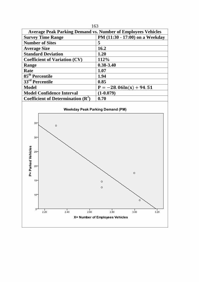
163
Average Peak Parking Demand vs. Number of Employees Vehicles
Survey Time Range PM (11:30 - 17:00) on a Weekday
Number of Sites 5
Average Size 16.2
Standard Deviation 1.20
Coefficient of Variation (CV) 112%
Range 0.38-3.40
Rate 1.07
85th
Percentile 1.94
33rd
Percentile 0.85
Model
Model Confidence Interval (1-0.079)
Coefficient of Determination (R2) 0.70

164
Average Peak Parking Demand vs. Number of Employees
Survey Time Range Weekday
Number of Sites 5
Average Size 34
Standard Deviation 0.31
Coefficient of Variation (CV) 59%
Range 0.20-0.97
Rate 0.52
85th
Percentile 0.81
33rd
Percentile 0.41
Model P= 20.88*e-.008x
Model Confidence Interval (1-0.793)
Coefficient of Determination (R2) 0.03

165
Average Peak Parking Demand vs. GFA (Square Meter)
Survey Time Range Weekday
Number of Sites 5
Average Size 1124
Standard Deviation 2.34
Coefficient of Variation (CV) 150%
Range 0.51-6.30
Rate 1.57
85th
Percentile 3.57
33rd
Percentile 1.11
Model P= 27502*X-1.072
Coefficient of Determination (R2) 0.93
Average Peak Parking Demand vs. GLA (per 100 Square Meter)
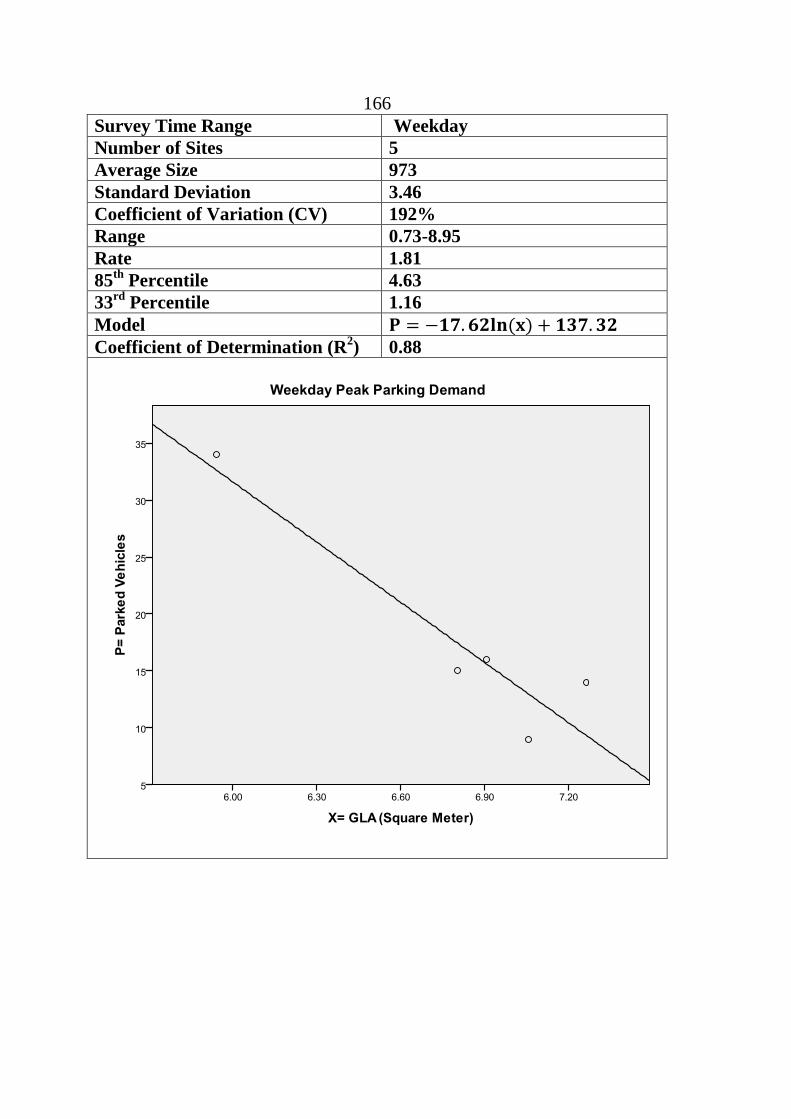
166
Survey Time Range Weekday
Number of Sites 5
Average Size 973
Standard Deviation 3.46
Coefficient of Variation (CV) 192%
Range 0.73-8.95
Rate 1.81
85th
Percentile 4.63
33rd
Percentile 1.16
Model
Coefficient of Determination (R2) 0.88

167
Average Peak Parking Demand vs. Number of Employees Vehicles
Survey Time Range Weekday
Number of Sites 5
Average Size 16.2
Standard Deviation 1.19
Coefficient of Variation (CV) 110%
Range 0.40-3.40
Rate 1.09
85th
Percentile 1.94
33rd
Percentile 0.88
Model
Coefficient of Determination (R2) 0.78

168
b. Institutional Office Class
Average Peak Parking Demand vs. Number of Employees
Survey Time Range AM (7:00 - 10:00) on a Weekday
Number of Sites 7
Average Size 209.8
Standard Deviation 0.40
Coefficient of Variation (CV) 88%
Range 0.31-1.42
Rate 0.45
85th
Percentile 0.88
33rd
Percentile 0.37
Model P= 0.478* X-5.269
Coefficient of Determination (R2) 0.96
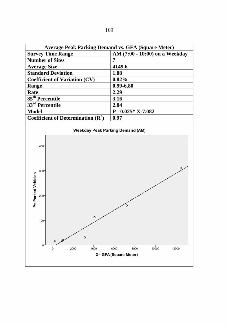
169
Average Peak Parking Demand vs. GFA (Square Meter)
Survey Time Range AM (7:00 - 10:00) on a Weekday
Number of Sites 7
Average Size 4149.6
Standard Deviation 1.88
Coefficient of Variation (CV) 0.82%
Range 0.99-6.80
Rate 2.29
85th
Percentile 3.16
33rd
Percentile 2.04
Model P= 0.025* X-7.082
Coefficient of Determination (R2) 0.97

170
Average Peak Parking Demand vs. GLA (per 100 Square Meter)
Survey Time Range AM (7:00 - 10:00) on a Weekday
Number of Sites 7
Average Size 4003.7
Standard Deviation 1.87
Coefficient of Variation (CV) 79%
Range 0.90-6.80
Rate 2.37
85th
Percentile 3.79
33rd
Percentile 2.21
Model P= 0.024* X-1.882
Coefficient of Determination (R2) 0.95

171
Average Peak Parking Demand vs. Number of Employees Vehicles
Survey Time Range AM (7:00 - 10:00) on a Weekday
Number of Sites 7
Average Size 104
Standard Deviation 0.53
Coefficient of Variation (CV) 0.58%
Range 0.56-2.13
Rate 0.91
85th
Percentile 1.23
33rd
Percentile 0.75
Model P= 15.502 e 0.012 x
Coefficient of Determination (R2) 0.98
Average Peak Parking Demand vs. Number of Employees

172
Survey Time Range PM (13:30 - 17:00) on a Weekday
Number of Sites 7
Average Size 209.8
Standard Deviation 0.22
Coefficient of Variation (CV) 48%
Range 0.26-0.96
Rate 0.46
85th
Percentile 0.60
33rd
Percentile 0.42
Model P=0.486* X-5.449
Coefficient of Determination (R2) 0.97

173
Average Peak Parking Demand vs. GFA (Square Meter)
Survey Time Range PM (13:30 - 17:00) on a Weekday
Number of Sites 7
Average Size 4149.6
Standard Deviation 1.20
Coefficient of Variation (CV) 51%
Range 1.22-4.60
Rate 2.33
85th
Percentile 3.27
33rd
Percentile 1.52
Model P=0.025* X-7.057
Coefficient of Determination (R2) 0.97
Average Peak Parking Demand vs. GLA (per 100 Square Meter)

174
Survey Time Range PM (13:30 - 17:00) on a Weekday
Number of Sites 7
Average Size 4003.7
Standard Deviation 1.26
Coefficient of Variation (CV) 52%
Range 1.40-4.60
Rate 2.41
85th
Percentile 3.98
33rd
Percentile 1.57
Model P=0.024* X-1.449
Coefficient of Determination (R2) 0.95

175
Average Peak Parking Demand vs. Number of Employees Vehicles
Survey Time Range PM (13:30 - 17:00) on a Weekday
Number of Sites 7
Average Size 104
Standard Deviation 0.32
Coefficient of Variation (CV) 34%
Range 0.46-1.44
Rate 0.33
85th
Percentile 1.17
33rd
Percentile 0.78
Model P=1.045* X-12.121
Coefficient of Determination (R2) 0.95
Average Peak Parking Demand vs. Number of Employees

176
Survey Time Range Weekday
Number of Sites 7
Average Size 209.8
Standard Deviation 0.38
Coefficient of Variation (CV) 79%
Range 0.37-1.42
Rate 0.48
85th
Percentile 0.88
33rd
Percentile 0.42
Model P= 0.48*X-0.57
Coefficient of Determination (R2) 0.97

177
Average Peak Parking Demand vs. GFA (Square Meter)
Survey Time Range Weekday
Number of Sites 7
Average Size 4149.6
Standard Deviation 1.82
Coefficient of Variation (CV) 75%
Range 1.52-6.80
Rate 2.41
85th
Percentile 3.49
33rd
Percentile 2.04
Model P= 0.025*X-2.18
Coefficient of Determination (R2) 0.97

178
Average Peak Parking Demand vs. GLA (per 100 Square Meter)
Survey Time Range Weekday
Number of Sites 7
Average Size 4003.7
Standard Deviation 1.81
Coefficient of Variation (CV) 73%
Range 1.52-6.80
Rate 2.50
85th
Percentile 4.20
33rd
Percentile 2.21
Model P= 0.024*X+ 3.26
Coefficient of Determination (R2) 0.95

179
Average Peak Parking Demand vs. Number of Employees Vehicles
Survey Time Range Weekday
Number of Sites 7
Average Size 104
Standard Deviation 0.49
Coefficient of Variation (CV) 1.24%
Range 0.67-2.13
Rate 0.96
85th
Percentile 1.24
33rd
Percentile 0.85
Model P= 1.03*X-7.17
Coefficient of Determination (R2) 0.95

180
c. Government Office Class
Average Peak Parking Demand vs. Number of Employees
Survey Time Range AM (7:00 - 9:00) on a Weekday
Number of Sites 14
Average Size 70.8
Standard Deviation 0.15
Coefficient of Variation (CV) 48%
Range 0.19-0.63
Rate 0.31
85th
Percentile 0.51
33rd
Percentile 0.26
Model
Coefficient of Determination (R2) 0.65
Average Peak Parking Demand vs. GFA (Square Meter)

181
Survey Time Range AM (7:00 - 9:00) on a Weekday
Number of Sites 14
Average Size 1400
Standard Deviation 1
Coefficient of Variation (CV) 65%
Range 0.96-4.75
Rate 1.55
85th
Percentile 2.66
33rd
Percentile 1.29
Model
Coefficient of Determination (R2) 0.54

182
Average Peak Parking Demand vs. GLA (per 100 Square Meter)
Survey Time Range AM (7:00 - 9:00) on a Weekday
Number of Sites 14
Average Size 1289.5
Standard Deviation 0.99
Coefficient of Variation (CV) 58%
Range 0.96-4.75
Rate 1.69
85th
Percentile 2.68
33rd
Percentile 1.72
Model
Coefficient of Determination (R2) 0.64
Average Peak Parking Demand vs. Number of Employees Vehicles

183
Survey Time Range AM (7:00 - 9:00) on a Weekday
Number of Sites 14
Average Size 23.6
Standard Deviation 0.30
Coefficient of Variation (CV) 33%
Range 0.33-1.57
Rate 0.92
85th
Percentile 1.25
33rd
Percentile 0.92
Model P= -0.312*X+ 23.903
Coefficient of Determination (R2) 0.78

184
Average Peak Parking Demand vs. Number of Employees
Survey Time Range PM (12:00- 16:00) on a Weekday
Number of Sites 14
Average Size 70.8
Standard Deviation 0.20
Coefficient of Variation (CV) 64%
Range 0.17-0.84
Rate 0.31
85th
Percentile 0.56
33rd
Percentile 0.27
Model P= 1.86*X 0.574
Coefficient of Determination (R2) 0.37

185
Average Peak Parking Demand vs. GFA (Square Meter)
Survey Time Range PM (12:00- 16:00) on a Weekday
Number of Sites 14
Average Size 1400
Standard Deviation 0.92
Coefficient of Variation (CV) 59%
Range 0.85-4.25
Rate 1.57
85th
Percentile 2.65
33rd
Percentile 1.51
Model
Coefficient of Determination (R2) 0.56

186
Average Peak Parking Demand vs. GLA (per 100 Square Meter)
Survey Time Range PM (12:00- 16:00) on a Weekday
Number of Sites 14
Average Size 1289.5
Standard Deviation 0.95
Coefficient of Variation (CV) 55%
Range 0.85-4.25
Rate 1.70
85th
Percentile 3
33rd
Percentile 1.57
Model P= 0.289*X 0.608
Coefficient of Determination (R2) 0.59

187
Average Peak Parking Demand vs. Number of Employees Vehicles
Survey Time Range PM (12:00- 16:00) on a Weekday
Number of Sites 14
Average Size 23.6
Standard Deviation 0.46
Coefficient of Variation (CV) 49%
Range 0.29-0.92
Rate 0.93
85th
Percentile 1.15
33rd
Percentile 0.92
Model P= 2.63*X 0.659
Coefficient of Determination (R2) 0.40

188
Average Peak Parking Demand vs. Number of Employees
Survey Time Range Weekday
Number of Sites 14
Average Size 70.8
Standard Deviation 0.19
Coefficient of Variation (CV) 58%
Range 0.19-0.84
Rate 0.33
85th
Percentile 0.56
33rd
Percentile 0.28
Model P=
Coefficient of Determination (R2) 0.46

189
Average Peak Parking Demand vs. GFA (Square Meter)
Survey Time Range Weekday
Number of Sites 14
Average Size 1400
Standard Deviation 0.99
Coefficient of Variation (CV) 59%
Range 0.96-4.75
Rate 1.68
85th
Percentile 2.78
33rd
Percentile 1.58
Model P=
Coefficient of Determination (R2) 0.61

190
Average Peak Parking Demand vs. GLA (per 100 Square Meter)
Survey Time Range Weekday
Number of Sites 14
Average Size 1289.5
Standard Deviation 1
Coefficient of Variation (CV) 55%
Range 0.96-4.75
Rate 1.82
85th
Percentile 3.01
33rd
Percentile 1.75
Model P=
Coefficient of Determination (R2) 0.64

191
Average Peak Parking Demand vs. Number of Employees Vehicles
Survey Time Range Weekday
Number of Sites 14
Average Size 23.6
Standard Deviation 0.61
Coefficient of Variation (CV) 52%
Range 0.43-3.0
Rate 1.17
85th
Percentile 1.32
33rd
Percentile 0.87
Model P= 2.8*X 0.664
Coefficient of Determination (R2) 0.43

192
17 Retail Land Use
a. Supermarket Retail Class
Average Peak Period Parking Demand vs. Number of Employees
Survey Time Range (7:00 - 22:00) on a Weekday
Number of Sites 15
Average Size 7.2
Standard Deviation 1.05
Coefficient of Variation (CV) 92%
Range 0.42-4.25
Rate 1.15
85th
Percentile 1.96
33rd
Percentile 0.89
Model P= 0.773*X+ 4.636
Coefficient of Determination (R2) 0.338

193
Average Peak Period Parking Demand vs. GLA (per 100 Square
Meter)
Survey Time Range (7:00 - 22:00) on a Weekday
Number of Sites 15
Average Size 448.8
Standard Deviation 1.74
Coefficient of Variation (CV) 83%
Range 0.83-6.0
Rate 2.08
85th
Percentile 5.13
33rd
Percentile 1.50
Model P= 0.014*X+ 3.74
Coefficient of Determination (R2) 0.509

194
Average Peak Period Parking Demand vs. Number of Employees
Vehicles
Survey Time Range (7:00 - 22:00) on a Weekday
Number of Sites 15
Average Size 2.53
Standard Deviation 5.93
Coefficient of Variation (CV) 152%
Range 0.90-18.50
Rate 3.91
85th
Percentile 11.53
33rd
Percentile 2.11
Model
Model Confidence Interval (1-0.313)
Coefficient of Determination (R2) 0.078

195
b. Strip Retail Class
Average Peak Period Parking Demand vs. Number of Employees
Survey Time Range (7:00 - 22:00) on a Weekday
Number of Sites 8
Average Size 11.5
Standard Deviation 0.51
Coefficient of Variation (CV) 63%
Range 0.50-2.10
Rate 0.82
85th
Percentile 1.03
33rd
Percentile 0.67
Model P= 0.492*X+ 4.843
Coefficient of Determination (R2) 0.678

196
Average Peak Period Parking Demand vs. GLA (per 100 Square
Meter)
Survey Time Range (7:00 - 22:00) on a Weekday
Number of Sites 8
Average Size 438.3
Standard Deviation 1.13
Coefficient of Variation (CV) 51%
Range 1.17-4.72
Rate 2.22
85th
Percentile 3.74
33rd
Percentile 2.71
Model P= 0.009*X+ 6.453
Coefficient of Determination (R2) 0.752

197
Average Peak Period Parking Demand vs. Number of Employees
Vehicles
Survey Time Range (7:00 - 22:00) on a Weekday
Number of Sites 8
Average Size 6.75
Standard Deviation 1.08
Coefficient of Variation (CV) 71%
Range 1-3.63
Rate 1.52
85th
Percentile 3.42
33rd
Percentile 1.21
Model P= 0.606*X+ 6.408
Model Confidence Interval (1-0.093)
Coefficient of Determination (R2) 0.40

198
Appendix (E): Residual Plots
18
19 Sample of Residual Plots
Attached Housing Land Use
20 AM Period
21 Independent Variable: Number of Occupied AH Units

199

200
22 Independent Variable: Number of Inhabitants

201
23 Independent Variable: Number of Occupied AH Units

202
24 Independent Variable: Number of Inhabitants

203
25 Detached Housing Land Use Class
26 Power Relationship
27 Independent Variable: Number of Occupied AH Units

204
28 Independent Variable: Number of Inhabitants

205
29 Independent Variable: Number of Occupied AH Units

206
30 Independent Variable: Number of Inhabitants

207
31 Apartment Housing Land Use Class
32 AM Period
33 Independent Variable: Number of Inhabitants

208
34 Independent Variable: GFA (sq. m.)

209
35 Independent Variable: Number of Occupied AH Units

210
36 PM Period
37 Independent Variable: Number of Inhabitants

211
38 Independent Variable: GFA (sq. m.)

212
39 Independent Variable: Number of Occupied AH Units
40

213
41 Office Land Use
42 General Office Land Use Class
43 Peak Period
44 Independent Variable: Number of Workers

214

215
45 Independent Variable: GFA (sq. m.)

216
46 Independent Variable: GLA (sq. m.)

217
47 Independent Variable: Workers Vehicles

218
48 AM Period
49 Independent Variable: Number of Workers
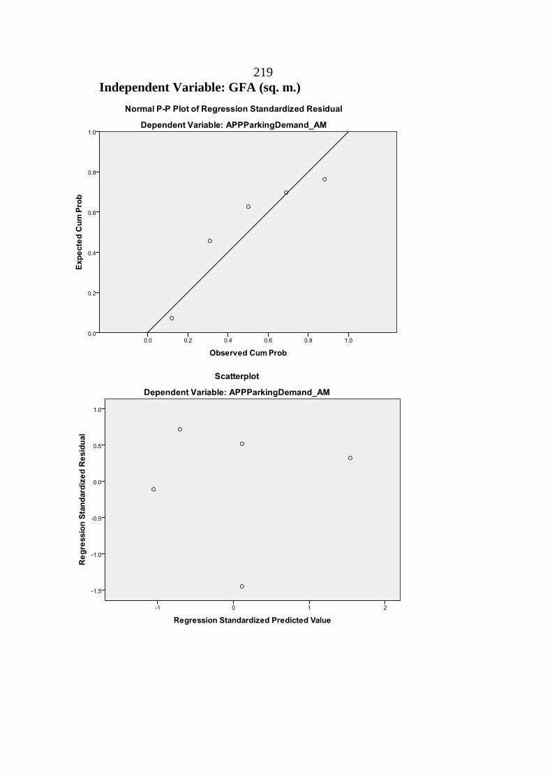
219
50 Independent Variable: GFA (sq. m.)

220
51 Independent Variable: GLA (sq. m.)

221
52 Independent Variable: Workers Vehicles

222
53 PM Period
54 Independent Variable: Number of Workers

223
55 Independent Variable: GFA (sq. m.)

224
56 Independent Variable: GLA (sq. m.)

225
57 Independent Variable: Workers Vehicles

226
58 Institutional Office Class
59 Peak
60 Independent Variable: Number of Workers
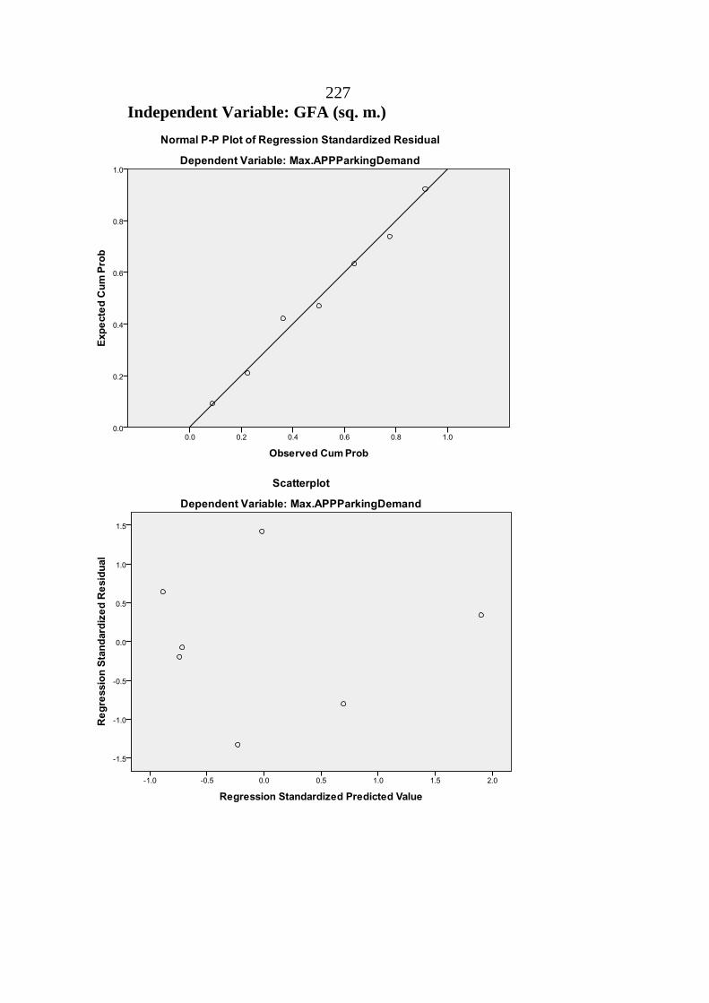
227
61 Independent Variable: GFA (sq. m.)

228
62 Independent Variable: GLA (sq .m.)

229
63 Independent Variable: Workers Vehicles

230
64 AM Period
65 Independent Variable: Number of Workers

231
66 Independent Variable: GFA (sq. m.)

232
67 Independent Variable: GLA (sq. m.)

233
68 Independent Variable: Workers Vehicles

234
69 PM Period
70 Independent Variable: Number of Workers
71 Independent Variable: GFA (sq. m.)

235
72 Independent Variable: GLA (sq. m.)

236
73 Independent Variable: Workers Vehicles

237
74 Government
75 Peak Period
76 Independent Variable: Number of Workers

238
77 Independent Variable: GFA (sq. m.)

239
78 Independent Variable: GLA (sq. m.)

240
79 Independent Variable: Workers Vehicles

241
80 AM Period
81 Independent Variable: Number of Workers

242
82 Independent Variable: GFA (s q. m.)

243
83 Independent Variable: GLA (sq. m.)

244
84 Independent Variable: Workers Vehicles

245
85 PM Period
86 Independent Variable: Number of Workers

246
87 Independent Variable: GFA (sq. m.)

247
88 Independent Variable: GLA (sq. m.)

248
89 Independent Variable: Workers Vehicles
90

249
91 Retail Land Use
92 Peak of Development/s
93 Supermarket Retail Class
94 Independent Variable: Workers

250

251
95 Independent Variable: GFA/GLA (sq. m.)
4

252
96 Independent Variable: Workers Vehicle

253
97 Strip Retail Class
98 Independent Variable: Workers

254
99 Independent Variable: GFA/GLA (sq. m.)

255
100 Independent Variable: Workers Vehicle

256
101 Appendix (F): Part of Palestinian Regulations

257

258

259

260

261

262
Vitae
Name : Jamil Mohammad Jamil Hamadneh
Nationality: Palestinian
Date of Birth: 23/6/1988
Email: [email protected]/ [email protected]
Address: Asira Ash-Shamlieh, Nablus. Palestine.
Academic Background: B. Sc. in Civil engineering at An-Najah National
University- Nablus City-Palestine. Bachelor Degree Graduation project is
in traffic engineering which is called "Building of Traffic Database for an
urban Roadways Network in Nablus CBD" including options for
improvements.


ب

ت
R2
(R2>0.6)