estimates of the trade and welfare e⁄ects of...

Estimates of the Trade and Welfare Effects of NAFTA

Lorenzo Caliendo∗

Yale University and NBER

Fernando Parro∗

Federal Reserve Board

July 24, 2014

Abstract

We build into a Ricardian model sectoral linkages, trade in intermediate goods, and sectoral hetero-

geneity in production to quantify the trade and welfare effects from tariff changes. We also propose a

new method to estimate sectoral trade elasticities consistent with any trade model that delivers a multi-

plicative gravity equation. We apply our model and use our estimated elasticities to identify the impact

of NAFTA’s tariff reductions. We find that Mexico’s welfare increases by 1.31%, U.S.’s welfare increases

by 0.08%, and Canada’s welfare declines by 0.06%. We find that intra-bloc trade increases by 118% for

Mexico, 11% for Canada and 41% for the U.S. We show that welfare effects from tariff reductions are

reduced when the structure of production does not take into account intermediate goods or input-output

linkages. Our results highlight the importance of sectoral heterogeneity, intermediate goods and sectoral

linkages for the quantification of the welfare gains from tariffs reductions.

JEL classifcation: F10, F11, F13, F14, F17.

Keywords: Trade policy, Gains from trade, Intermediate inputs, Sectoral interrelations, Computa-

tional general equilibrium.

∗First Draft: November 2009. We are particularly grateful to Robert Lucas, Samuel Kortum, Nancy Stokey for theircontinuous encouragement, support and advice. We also thank for helpful comments Fernando Alvarez, Costas Arkolakis, KyleBagwell, Francesco Caselli, Thomas Chaney, Dave Donaldson, Jonathan Eaton, Rob Feenstra, Cecilia Fieler, Gordon Hanson,Timothy Kehoe, Kalina Manova, Brent Neiman, Ralph Ossa, Stephen Redding, John Romalis, Peter Schott, Robert Shimer,Bob Staiger, Daniel Sturm, Chang Tai Hsieh, Silvana Tenreyro, four anonymous referees, and many seminar participantsfor useful conversations and comments. We thank Zina Saijid for excellent research assistance. Correspondence: Caliendo,[email protected], Parro, [email protected]. The views in this paper are solely the responsibility of the authorsand should not be interpreted as re‡ecting the views of the Board of Governors of the Federal Reserve System or of any otherperson associated with the Federal Reserve System.

1

© The Author 2014. Published by Oxford University Press on behalf of The Review of

Economic Studies Limited.

The Review of Economic Studies Advance Access published November 14, 2014 at Y

ale University on O

ctober 2, 2015http://restud.oxfordjournals.org/

Dow

nloaded from

http://restud.oxfordjournals.org/

1. INTRODUCTION

Sectors and countries are interrelated. When the U.S. reduces tariffs applied to Mexico in a given sector,

it not only affects prices in that industry but also in sectors that purchase materials from that industry.

Moreover, a tariff reduction affects prices in non-tradable sectors that are using inputs from tradable sectors.

Of course, how important are these direct and indirect effects from tariff changes will depend on the extent to

which sectors are interrelated. For instance, the larger is the share of tradable goods used in the production

of non-tradable goods the larger are the gains for producers of non-tradable goods from a reduction in the

price of tradables. Even more, if non-tradable goods are also used as inputs in the production of other goods,

or as final goods in consumption, then the benefits spread to the rest of the economy. In fact, most of the

final goods consumed are non-tradable goods.1 However, recent developments in international trade pay

little attention to understanding how the gains from tariff reductions spread across sectors.2

In this paper, we build into a multi-country, multi-sector Ricardian model the interaction across tradable

and non-tradable sectors observed in the input-output tables. We use the model to identify the trade and

welfare effects of tariff reductions from the North American Free Trade Agreement (NAFTA) between Mexico,

Canada and the U.S. NAFTA provides a unique example to quantify the trade and welfare effects of tariff

changes for three main reasons. First, it is among the largest free trade area in the world, both in terms of

population and GDP; second, it involves countries with very different structures of production, reflected by

their GDP per capita and different sectoral specialization of economic activity; and third, it is an archetypal

agreement that resulted in the creation of a cross-border production chain, as revealed by the large share

of intermediate goods and intra-industry trade across members.3 These features are the key characteristics

from NAFTA that help us understand more broadly the quantitative importance of sectoral heterogeneity,

trade in intermediate goods, and sectoral linkages.

Adding more detail into a model comes at the cost of losing track of the mechanisms that deliver the main

results. In fact, this complexity has lead to criticism of computational general equilibrium (CGE) models

in the past.4 To address this issue we build on the seminal work of Eaton and Kortum (2002) to develop a

tractable and simple model for tariff policy evaluation that escapes the black box denigration of traditional

CGE models. As a result, we can decompose and quantify the differential role that intermediate goods and

sectoral linkages have as amplifiers of the gains from tariff reductions. We also show that regardless of the

number of sectors and how complicated the interactions across sectors are, the model can be reduced to a

system of one equation per country, and the solution depends on estimates of one set of parameters, the

dispersion of productivity across sectors (trade elasticities). Our solution method simplifies considerably the

1Non-tradable goods (services) accounted for more than 80% of the total final goods demanded in the year 1993 for the U.S.2An exception is the work of Arkolakis, Costinot, and Rodriguez-Clare (2012) where they evaluate the welfare gains from

trade openness implied by a variety of international trade models including multi-sector models.3 In Section 2 we document that sectoral trade in intermediate goods is particularly important for NAFTA members.4These models have been criticized for their complexity, lack of transparency and analytical foundations, and the arbitrary

choice of the value of key parameters (Baldwin and Venables 1995 describe them as “black boxes”).

2

at Yale U

niversity on October 2, 2015

http://restud.oxfordjournals.org/D

ownloaded from


data requirements and estimated parameters needed for the evaluation of tariff changes.

In our theory, production is at constant returns to scale and markets are perfectly competitive. Countries

import intermediate goods subject to trade costs from the lowest cost supplier in the world.5 Intermediate

goods in a given sector are used for the production of a sectoral good which is then used as final good for

consumption and as material in the production of tradable and non-tradable intermediate goods from all

sectors. Productivity differences across individual producers in a sector are introduced in the same way as

in Eaton and Kortum (2002). The larger is the dispersion of productivities across producers, the larger

are the gains from trade integration. In our model, productivity, as well as the dispersion of productivity,

varies across sectors. This heterogeneity in the dispersion of productivities together with the share of

intermediate goods in production and sectoral interrelations are key in order to capture how a tariff reduction

has differential impact across sectors.

We express the model in relative changes and identify the trade and welfare effects of NAFTA’s tariff

reductions.6 Our simulations are performed with few data and parameter requirements. In particular, we

only use data on bilateral trade flows, production, tariffs and an estimate of sectoral trade elasticities. We

develop a new method to estimate sectoral trade elasticities. The estimations are performed using trade and

tariff data, without assuming bilaterally symmetric trade costs as is standard in the literature. Moreover,

the method is consistent with any trade model that delivers a gravity-type trade equation. We estimate

the parameters of the model at a sectoral level using data from 1993, the year before NAFTA went into

effect. We calibrate a 31 countries 40 sector version of our model. Then, using the estimated parameters and

incorporating the change in tariffs from 1993 to 2005, both between NAFTA members and with the rest of

the world, we use the model to evaluate the welfare effects and quantify the changes in exports and imports

in aggregate and at the sectoral level.

We find that NAFTA’s tariffs reductions had a considerable impact on its member’s economies, in partic-

ular for Mexico. NAFTA augmented aggregate intra-bloc trade by 118% for Mexico, 11% for Canada and

41% for the U.S. We find that NAFTA increased the sectoral specialization of export activity in Mexico.

After NAFTA the most export oriented sector in Mexico (Electrical Machinery) represented one third of the

total export shares, while before it was only one fifth. For the case of Canada and U.S. the result is different;

sectoral concentration of export activity was reduced.

We find that not all countries gained from NAFTA. Mexico and the U.S. gained 1.31% and 0.08% respec-

5The importance of trade in intermediate goods has been documented by several studies. For instance, Feenstra and Hanson(1996) find that the share of imported intermediates increased from 5.3% of total U.S. intermediate purchases to 11.6% between1972 and 1990. Campa and Goldberg (1997) find similar evidence for Canada and the United Kingdom. Hummels, Ishii, andYi (2001), and Yeats (2001) show that international trade in intermediate inputs has increased more than that in final goods.

6We perform a model-based identification of the trade effects due to NAFTA’s tariff reductions by holding technology andother trade costs fixed. By doing this, we are not saying that technology or other trade costs might not have changed as aconsequence of the change in tariffs. We are agnostic about how they might have changed and focus instead on the direct effectof tariff changes over the allocation of resources. An alternative exercise could have been to quantify the implied changes intechnology and other trade costs in order for the model to deliver the observed change in trade flows after NAFTA. But theproblem there is how to identify if these changes were due only to NAFTA. Unless a model of TFP or trade costs is writtenthere is no hope for identification. In our case, we take as exogenous the observable change in tariff due to NAFTA to quantifythe trade effects.

3

at Yale U



ownloaded from


tively, while Canada suffered a welfare loss of 0.06%. Still, real wages increased for all NAFTA members

and Mexico had the largest gains. We decompose the welfare effects into terms of trade and volume of trade

effects and find that most of the gains from NAFTA are a result of an increase in the volume of trade. We

find that the trade created, mostly between NAFTA members, was larger than the trade diverted from other

economies. This was particularly so for Mexico and Canada. The welfare gains from trade creation with

NAFTA members are 1.80% and 0.08% while the welfare loss from trade diversion with the rest of the world

are 0.08%, and 0.04% for Mexico and Canada respectively. Only a handful of sectors were responsible for

the aggregate volume of trade effects. These were sectors highly protected before NAFTA, like Textiles in

Mexico, with a large trade elasticity, like Petroleum, and with a large share of material use and sectoral

interdependence, like Electrical Machinery and Autos.

The terms of trade effects were mixed. We find that Mexico’s and Canada’s terms of trade deteriorated by

0.41% and 0.11%, respectively, mostly due to reductions in export prices, while for the U.S. terms of trade

increased by 0.04%; largely attributed to cheaper import prices from Mexico. We also decompose the terms

of trade effects by sector and find that terms of trade effects were primarily concentrated in a few sectors.

We show that certain sectors had a larger aggregate effect compared to others depending on the magnitude

of sectoral reductions in import tariffs, the share of materials used in production, and sectoral linkages.

We also evaluate the welfare effects from observed world tariff changes. We find that all countries in the

world gained. The welfare gains for NAFTA members were 1.36%, 0.10% and 0.22% for Mexico, Canada

and the U.S. Netting out the effect of NAFTA, these figures show that Canada was the largest winner from

world tariff reductions, followed by U.S. and then Mexico.

Finally, we quantify the trade and welfare effects from NAFTA’s tariff reductions across different class of

models. We find that welfare effects are on average 71% lower in a one sector model, 62% lower in a model

without materials, and 50% lower in a model without sectoral linkages. Trade effects are reduced on average

50%, 26%, and 18%, respectively. These results confirm that sectoral heterogeneity, intermediate inputs,

and sectoral linkages are important mechanisms to quantify the trade and welfare effects from tariff changes.

Quantifying potential welfare gains and costs from trade policies has become increasingly important over

the years.7 Our paper relates to a large literature that evaluates trade policy and is mostly related to studies

that quantify the gains from trade from NAFTA.8 In particular, Anderson and van Wincoop (2002) who use

a one good gravity model to evaluate the gains from NAFTA. Relative to Anderson and van Wincoop (2002)

7The number of regional trade agreements (RTAs) signed in the world has increased dramatically in the last 20 years. In1990 there were close to 25 RTAs signed, by 2010 more than 180. By the year 2002 more than one third of world trade wascovered by RTAs.

8Jacob Viner’s (1950) work was among the first to study the welfare analysis of trade policy. Bhagwati, Krishna, andPanagariya (1999) put together many of the major theoretical contributions since Viner. More recents are Anderson and vanWincoop (2004), Baier and Bergstrand (2009), Deardorff (1998), Redding and Venables (2004), Rose (2004), and Subramanianand Wei (2007). Bagwell and Staiger (2010) survey recent economic research on trade agreements, with special focus on theGATT/WTO. Several studies have focused on the case of NAFTA, for instance Krueger (1999) and the references therein,Lederman, Maloney, and Serven (2005), Romalis (2007), and Trefler (2006). For results on CGE models in general see Brown,Deardorff, and Stern (1994), Brown and Stern (1989), Kehoe and Kehoe (1994), and for the case of NAFTA refer to Fox (1999),Kehoe (2003), Rolleigh (2008) and Shikher (2010).

4

at Yale U



ownloaded from


our model has multiple sectors, intermediate goods trade, a production economy, non-tradable sectors and

builds on Ricardian motives of trade instead of love from variety.9 Our results show that these features are

quantitatively important.

Our paper is closely related to a recent and growing literature that extends the Eaton and Kortum (2002)

model to multiple-sectors. For instance Arkolakis, et al. (2012), Caliendo and Parro (2010), Chor (2010),

Costinot, Donaldson, and Komunjer (2012), Donaldson (2012), Dekle, Eaton and Kortum (2008), Eaton,

Kortum, Neiman, and Romalis (2011), Hsieh and Ossa (2011), and Shikher (2011).10 Our paper differs

from these studies in several dimensions. First, we explicitly consider sectoral linkages between tradable

sectors and between tradable and non-tradable sectors unlike previous Ricardian trade models. In our

model, producers of non-tradable goods differ in productivity levels, demand tradable and non-tradable

intermediate goods for production and supply goods not only for consumption but also for production in

all sectors.11 This feedback in production turns out to be important in order to quantify the trade and

welfare effects of tariff reductions. Second, we show how accounting for intermediate goods in production

and sectoral linkages does amplify the trade and welfare effects of trade costs and tariff reductions.12 Third,

we extend the Ricardian model to perform a thoroughly quantitative evaluation of the trade and welfare

effects from changes in trade policies. Finally, the way in which we take the model to the data is very

different compared to other studies. We solve the multi-country and multi-sector model in changes, relative

to a base year, allowing us to perform counterfactuals without relying on estimates of unobserved structural

parameters, like fundamental productivity. We show that this approach is simple and useful in order to

evaluate counterfactual changes in trade costs more broadly.

Our paper is also related to studies that propose new methods to estimate trade elasticities.13 We propose a

new method that identifies sectoral and aggregate trade elasticities by exploiting the cross sectional variation

in trade shares induced by the cross sectional variation in tariffs. The method relies on the multiplicative

properties of the gravity equation consistent with a large variety of trade models (Krugman 1981, Eaton and

Kortum 2002, Anderson and Wincoop 2003, Melitz 2003, and Chaney 2008).

The paper is structured as follows. In Section 2 we motivate the importance of modeling trade in in-

termediates, multiple sectors, and sectoral linkages for tariff policy evaluation. In Section 3, we develop a

methodology to evaluate the trade and welfare effects of tariff changes, we present the equilibrium conditions

9This last distinction is important since it generates changes at the extensive margin of trade while this is not the case ofan Armington type model as commonly used in CGE analysis.10The Eaton and Kortum (2002) model has been extended in many other directions also. One of the earliest studies was Yi

(2003) who uses the model to understand if vertical specialization can explain the large growth in trade. More recent studiesare Burstein, Cravino, and Vogel (2013), Burstein and Vogel (2012), Caselli, Koren, Lisicky, and Tenreyro (2012), Fieler (2011),Kerr (2009), Levchenko and Zhang (2011), Parro (2013), Ossa (2012), Ramondo and Rodriguez-Clare (2013), and Waugh(2010). For a comprehensive survey of recent extensions of the Ricardian model of trade refer to Eaton and Kortum (2012).11Non-tradable good sectors are often modeled as an outside sector that does not use intermediate goods for production. For

example see Alvarez and Lucas (2007).12 In Section 5.3 we compare the effects of NAFTA across different models and show that sectoral heterogeneity, intermediate

goods, and sectoral linkages are quantitatively important.13For instance, Feenstra (1994), Head and Ries (2001), Anderson and van Wincoop (2004) and references therein, Romalis

(2007), Simonovska and Waugh (2013) and Bergstrand, Egger, and Larch (2013).

5

at Yale U



ownloaded from


of the model, and show how to solve and calibrate the model. In Section 4, we propose a new method and

estimate sectoral trade elasticities. In Section 5, we apply the model to evaluate the trade and welfare effects

of NAFTA. In Section 6 we conclude.

2. TARIFFS, INTERMEDIATE GOODS AND SECTORAL LINKAGES

In this section we motivate the importance of modeling trade in intermediates, multiple sectors, and

sectoral linkages for tariff policy evaluation. The Appendix “Data Sources and Description”, at the end

of the document, describes in detail the data sources that we use in this paper. Throughout the paper,

whenever we make reference to a sector in the data, we refer to a 2-digit ISIC Rev. 3 industry. Table A.1 in

the Appendix “Data Sources and Description”provides a description of the sectoral categories.

Tariff rates vary substantially across sectors. In 1993, the year before NAFTA went into effect, sectoral

tariff rates applied by Mexico, Canada and the U.S. to NAFTA members were, on average, 12.5%, 4.2%,

and 2.7%, respectively, with a large heterogeneity across sectors (Figure A.1, in the appendix, presents the

effective tariffs rates across NAFTA members for the year 1993). By 2005 they dropped almost to zero

between NAFTA members, but tariffs that Mexico, Canada and the U. S. applied to the rest of the world

were, on average, 7.1%, 2.2%, and 1.7%, respectively.14 The fact to take away is that by 2005 average tariffs

had decreased considerably, but they still remained very dispersed across sectors. Trade and welfare effects

of average changes in tariffs can be analyzed using a one-sector trade model; however, the effects of changes

in the dispersion of tariffs can only be analyzed with a model that includes multiple sectors, sectoral linkages

and intermediate goods.

Actually, most goods traded are intermediate goods.15 In 1993, 68% of Mexico’s imports from countries

not belonging to NAFTA were intermediate goods. The share for Canada is 61.5% and for the U.S. 64.6%.

Intermediate goods trade is even more important for NAFTA members. In fact, 82,1% of Mexico’s imports

from NAFTA were intermediate goods, while for Canada and the U.S. the values were 72.3% and 72.8%

respectively. Therefore, by 1993 most goods traded across NAFTA members were intermediate goods and

trade of these types of goods was more important across NAFTA members than with the rest of the world.

Also, tradable and non-tradable sectors are interconnected. Using input-output (I-O) tables we can mea-

sure the proportion of spending from sectors on final and intermediate goods from other sectors. One salient

characteristic of any I-O matrix is that it presents a strong diagonal, namely that the share of own industry

material inputs purchased are important. However, this expenditure share is far from 100%. For example,

14The reason why tariffs decreased is mostly that several free trade agreements entered into force during the period 1993-2005.For instance, Mexico signed free trade agreements with Costa Rica in 1995, Nicaragua in 1998, Chile in 1999, the EuropeanUnion in 2000, El Salvador, Guatemala and Honduras in 2001, and Japan in 2005; Canada signed agreements with Chile in1997 and Costa Rica in 2002; and the United States signed agreements with Jordan in 2001, Chile, Costa Rica, the DominicanRepublic, El Salvador, Guatemala, Honduras, Nicaragua and Singapore in 2004, and Australia in 2005.15The descriptive statistics presented in this paragraph use data from COMTRADE via WITS. The product categories are the

HS Standard Product Groups, UNCTAD. We refer to intermediate goods to categories UNCTAD-SoP2 and UNCTAD-SoP4.The intermediate goods traded in the model that we present below map to these two categories.

6

at Yale U



ownloaded from


for the U.S., the mean diagonal share is 16% and has a standard deviation of 15%, while for Mexico, the

mean diagonal share is 13% and has a standard deviation of 14%.16 If we focus only on tradable sectors,

the mean share of the diagonal elements is 20%, and 19% while the mean share of the diagonal elements for

the non-tradable sectors are 11% and 7%, respectively for the U.S. and Mexico. This means that industries

purchase mostly intermediate inputs from other industries.17 Moreover, I-O tables reflect that tradable

and non-tradable sectors are interrelated. The average share of tradable sectors in the production of non-

tradable sectors is 23% for the U.S. and 32% for Mexico, while the average share of non-tradable sectors in

the production of tradable sectors is 34% for the U.S. and 26% for Mexico. This casual inspection of the I-O

tables shows that sectors are strongly interrelated and that non-tradable sectors are a relevant input in the

production of tradables and vice versa.

We finish this subsection concluding that an assessment of the economics effects of NAFTA needs to

take into account that most goods traded are intermediate goods, that countries have different structure

of production and that there is substantial sectoral heterogeneity in tariffs. We now proceed to describe a

model that takes all of these mechanisms into account.

3. A QUANTITATIVE MODEL FOR TRADE POLICY EVALUATION

We develop a quantitative general equilibrium model with trade in intermediate goods, sectoral hetero-

geneity and input-output linkages, that takes into consideration all the empirical facts described in the

previous section. The model builds on the Ricardian trade model of Eaton and Kortum (2002). There are

N countries and J sectors. We denote countries by i and n and sectors by j and k. Sectors are of two types,

either tradable or non-tradable and there is only one factor of production, labor. All markets are perfectly

competitive and labor is mobile across sectors and not mobile across countries.

3.1 The Model

3.1.1 Households.–

In each country there are a measure of Ln representative households that maximize utility by consuming

final goods Cjn. The preferences of the households are given by

u (Cn) =∏J

j=1Cj αjnn , where

∑J

j=1αjn = 1. (1)

We denote by In households’ income. Income is derived from two sources; households supply labor Ln

at a wage wn and receive transfers on a lump-sum basis (tariff revenues and transfers from the rest of the

world, as we will see in a moment).

16These figures are computed using the I-O tables described in the Appendix “Data Sources and Description.”17Jones (2007) presents a detailed description of the characteristics of I-O tables. He shows that, regardless of the level of

sectoral disaggregation, the largest share is always the share of own industry material inputs purchased. However, the higherthe level of disaggregation, the smaller the share is. For instance, the share of own industry material inputs purchased are, onaverage, 3.3% of total material purchases for the case of the U.S. using a 6-digit I-O table.

7

at Yale U



ownloaded from


3.1.2 Intermediate goods.–

A continuum of intermediate goods ωj ∈ [0, 1] is produced in each sector j. Two types of inputs, labor and

composite intermediate goods (also referred to as materials) from all sectors, are used for the production of

each ωj . Producers of intermediate goods across countries differ in the effi ciency of production. We denote

by zjn(ωj)the effi ciency of producing intermediate good ωj in country n. The production technology of a

good ωj is

qjn(ωj) = zjn(ωj) [ljn(ωj)

]γjn∏J

k=1

[mk,jn (ωj)

]γk,jn ,

where ljn(ωj) is labor andmk,jn (ωj) are the composite intermediate goods from sector k used for the production

of intermediate good ωj . The parameter γk,jn > 0 is the share of materials from sector k used in the production

of intermediate good ωj , with∑Jk=1 γ

k,jn = 1 − γjn, and the parameter γjn > 0 is the share of value added.

Both value added shares and intermediate goods shares vary across countries and sectors.18

Since production of intermediate goods is at constant returns to scale and markets are perfectly competi-

tive, firms price at unit cost, cjn/zjn

(ωj), where cjn denotes the cost of an input bundle. In particular

cjn = Υjnw

γjnn

∏J

k=1Pk γk,jnn , (2)

where P kn is the price of a composite intermediate good from sector k, and Υjn is a constant.

19 Equation (2)

captures a key difference compared to the one-sector model or the multi-sector model without interrelated

sectors, as the cost of the input bundle depends on wages and on the price of all the composite intermediate

goods in the economy, tradable and non-tradable. A change in policy that affects the price in any single

sector will affect indirectly all the sectors in the economy via the input bundle. We show later that this

interrelation plays an important role in evaluating the trade and welfare effects from trade openness.

3.1.3 Composite intermediate goods.–

Producers of composite intermediate goods in sector j and country n, supply Qjn at minimum cost by pur-

chasing intermediate goods ωj from the lowest cost suppliers across countries.20 The production technology

18The main reason why we assume a unit elasticity of substitution across materials is because, at the level of aggregation atwhich we conduct our empirical analysis, value added and I-O shares are fairly constant over time. Using I-O tables for theyears 1995 and 2005, at the two-digit ISIC rev 2, from 26 countries sourced from WIOD (http://www.wiod.org/), we evaluatedthe stability of input shares by calculating the correlation coeffi cient across all input shares over time. We find that for allcountries, the correlation was higher than 0.91. Still, Appendix “CES Model”presents a general version of our model where weallow for any degree of substitutability across inputs.

19Specifically, Υjn ≡∏J

k=1(γk,jn )−γ

k,jn (γjn)−γ

jn .

20Allowing for producers of composite intermediate goods to search for the lowest cost supplier is a key distinction frommodels with Armington-type assumptions. In those models, because of the love for variety, regardless of the price, goods arealways bought from all sources, since they are differentiated by country of origin. In the Eaton and Kortum (2002) model, thesource from which goods are purchased is endogenously determined and can change as a consequence of tariff reductions. Thisis crucial in order to understand why this model conceptually takes into account changes at the extensive new goods marginand not only changes at the intensive old goods margin, as is the case in Armington-type models. However, both models deliversimilar aggregate moments for trade flows. In fact, the gravity equation implied from the Eaton and Kortum (2002) model,equation (6) below, is identical to the Armington model after mapping the dispersion of productivity, θ, and the technologyparameter, λ, to the elasticity of substitution and the home bias parameter in the Armington-type models.

8

at Yale U



ownloaded from


of Qjn is an Ethier (1982) or Dixit and Stiglitz (1977) aggregator given by

Qjn =

[∫rjn(ωj)1−1/σjdωj

]σj/(σj−1),

where σj > 0 is the elasticity of substitution across intermediate goods within sector j, and rjn(ωj) is the

demand of intermediate goods ωj from the lowest cost supplier. The solution to the problem of the composite

intermediate good producer gives the following demand for good ωj

rjn(ωj) =

(pjn(ωj)

P jn

)−σjQjn,

where P jn is unit price of the composite intermediate good

P jn =

[∫pjn(ωj)1−σjdωj

] 1

1−σj

,

and pjn(ωj) denotes the lowest price of intermediate good ωj across all locations n.

Composite intermediate goods from sector j are used as materials for the production of intermediate good

ωk in the amount mj,kn (ωk) in all sectors k, and as final goods in consumption Cjn.

21

3.1.4 International trade costs and prices.–

We assume that trade in goods is costly. In particular, there are two types of trade costs: iceberg trade

costs and an ad-valorem flat-rate tariffs. Iceberg costs are defined in physical units as in Samuelson (1954),

where one unit of a tradable intermediate good in sector j shipped from country i to country n requires

producing djni ≥ 1 units in i, with djnn = 1. Goods imported by country n from country i have to pay an

ad-valorem flat-rate tariff τ jni applicable over unit prices. We combine both trade costs, represented by

κjni = τ jnidjni, (3)

where τ jni = (1 + τ jni). We also assume that the triangular inequality holds; κjnhκ

jhi > κjni for all n, h, i.

After taking into account trade costs, a unit of a tradable intermediate good ωj produced in country i is

available in country n at unit prices cjiκjni/z

ji

(ωj). Therefore, the price of intermediate good ωj in country

n is given by

pjn(ωj)

= mini

cjiκ

jni

zji (ωj)

.

We model non-tradable sectors in the same way as tradable sectors but impose that κjin =∞; thus, in some

sectors goods are not traded because it is always cheaper to buy goods from local suppliers. In non-tradable

sectors, pjn(ωj)

= cjn/zjn

(ωj)and the demand of intermediate goods is given by rjn(ωj) = qjn(ωj).

Ricardian motives to trade are introduced following Eaton and Kortum’s (2002) probabilistic representa-

tion of technologies allowing productivities to differ by country and also by sectors. In particular, we assume21The market clearing condition for the composite intermediate good in sector j is

Qjn = Cjn +∑J

k=1

∫mj,kn (ωk)dωk.

9

at Yale U



ownloaded from


that the effi ciency of producing a good ωj in country n is the realization of a Fréchet distribution with a

location parameter that varies by country and sector, λjn > 0 and shape parameter that varies by sector,

θj .22 In the context of this model, a higher λjn makes the average productivity in a sector higher, a notion

of absolute advantage, while a smaller value of θj implies a higher dispersion of productivity across goods

ωj , a notion of comparative advantage. We assume that the distributions of productivities are independent

across goods, sectors and countries, and that 1 + θj > σj . With these assumptions on the distribution of

effi ciencies we can solve for the distribution of prices.23 The price of the composite intermediate good is then

given by

P jn = Aj[∑N

i=1λji (c

jiκjni)−θj]−1/θj

, (4)

for all sectors j and countries n; where Aj is a constant. Note that (4) is also the price index of the

non-tradable goods sector. The difference is that in that case, since κjin = ∞, the price index is given by

P jn = Ajλj −1/θj

n cjn.

Consumers purchase final goods at prices P jn. With Cobb-Douglas preferences (1), the consumption price

index is given by

Pn =∏J

j=1(P jn/α

jn)α

jn . (5)

3.1.5 Expenditure shares.–

Total expenditure on sector j goods in country n is given by Xjn = P jnQ

jn. We denote by X

jni to the

expenditure in country n of sector j goods from country i. It follows that country n′s share of expenditure

on goods from i are given by πjni = Xjni/X

jn. Using the properties of the Fréchet distribution we can derive

expenditure shares as a function of technologies, prices and trade costs

πjni =λji

[cjiκ

jni

]−θj∑N

h=1λjh

[cjhκ

jnh

]−θj . (6)

As we can see, bilateral trade shares πjni take the form of a multi-sector version of a gravity equation.

Changes in tariffs have a direct effect in trade shares via κjni, and from (2) note that changes in tariffs also

have an indirect effect through the input bundle cji since it incorporates all the information contained in the

I-O tables.

3.1.6 Total expenditure and trade balance.–

Total expenditure on goods j is the sum of the expenditure on composite intermediate goods by firms and

22For a description of the properties of the Fréchet distribution, refer to Eaton and Kortum (2002). Donaldson (2012) relatesthis assumption to other standard assumptions used in models of international trade with heterogeneous firms, like those inMelitz (2003), Chaney (2008), and others. Costinot et al. (2012) consider the case of more general distributions.23Appendix “Distribution of Prices and Expenditure Shares” presents a detailed derivation of the distribution of prices and

how to solve for the price index (4) as well as the expenditure shares (6). The derivation follows Eaton and Kortum (2002)applied to a multi-sector economy.

10

at Yale U



ownloaded from


the expenditure by households. Then, Xjn is given by

Xjn =

∑J

k=1γj,kn

∑N

i=1Xki

πkin1 + τkin

+ αjnIn, (7)

where

In = wnLn +Rn +Dn, (8)

represents final absorption in country n, as the sum of labor income, trade deficit, and tariff revenues. In

particular, Rn =∑Jj=1

∑Ni=1 τ

jniM

jni where M

jni = Xj

nπjni

1+τjniare country n′s imports of sector j goods from

country i. The summation of trade deficits across countries is zero,∑Nn=1Dn = 0, and national deficits are the

summation of sectoral deficits,Dn =∑Jk=1D

kn. Sectoral deficits are defined byD

jn =

∑N

i=1M jni−

∑N

i=1Ejni,

where Ejni = Xji

πjin1+τjin

are country n′s exports of sector j goods to country i. Aggregate trade deficits in

each country are exogenous in the model, however sectoral trade deficits are endogenously determined.

Finally, using the definition of expenditure and trade deficit we have that

∑J

j=1

∑N

i=1Xjn

πjni1 + τ jni

−Dn =∑J

j=1

∑N

i=1Xji

πjin1 + τ jin

. (9)

This condition reflects the fact that total expenditure, excluding tariff payments, in countryn minus trade

deficits equals the sum of each country’s total expenditure, excluding tariff payments, on tradable goods from

country n. We are adding over all sectors whether a sector is tradable or non-tradable. The non-tradable

sectors will appear in both sides of the equation and cancel out.24

We now define formally the equilibrium under policies τ jni in this model.

Definition 1 Given Ln, Dn, λjn and d

jni, an equilibrium under tariff structure τ is a wage vector w ∈ RN

++

and pricesP jnJ,Nj=1,n=1

that satisfy equilibrium conditions (2) , (4) , (6) , (7) , and (9) for all j, n.

3.1.6 Equilibrium in relative changes.–

Instead of solving for an equilibrium under policy τ we solve for changes in prices and wages after changing

from policy τ to policy τ ′, what we define as an equilibrium in relative changes.25 There are several advantages

of doing so. First, we can match exactly the model to the data in a base year; second, we can identify the

effect on equilibrium outcomes from a pure change in tariffs, which is what we are after in this paper; and

finally we can solve for the general equilibrium of the model without needing to estimate parameters which

are diffi cult to identify in the data, as productivities λjn and iceberg trade costs djni.

We now define the equilibrium of the model under policy τ ′ relative to a policy under tariff structure τ .

24 It is also possible to show that (9) implies labor market clearing. To see this, add (7) across sectors and substitute into (9)to obtain

wnLn =∑J

j=1γjn∑N

i=1Xji

πjin

1 + τ jin.

25This idea of expressing the equilibrium in relative changes follows Dekle et al. (2008). They use it to understand the effectsof a change in trade deficits while we use it to compute the effects of a change in the tariff structure.

11

at Yale U



ownloaded from


Definition 2 Let (w, P ) be an equilibrium under tariff structure τ and let (w′, P ′) be an equilibrium under

tariff structure τ ′. Define(w, P

)as an equilibrium under τ ′ relative to τ , where a variable with a hat “x”

represents the relative change of the variable, namely x = x′/x. Using (2) , (4) , (6) , (7) , and (9) the

equilibrium conditions in relative changes satisfy:

Cost of the input bundles:

cjn = wγjnn

∏J

k=1P kn

γk,jn . (10)

Price index:

P jn =

[∑N

i=1πjni[κ

jnic

ji ]−θj]−1/θj

. (11)

Bilateral trade shares:

πjni =

[cji κ

jni

P jn

]−θj. (12)

Total expenditure in each country n and sector j:

Xj′

n =∑J

k=1γj,kn

∑N

i=1

πk′

in

1 + τk′in

Xk′

i + αjnI′n. (13)

Trade balance: ∑J

j=1

∑N

i=1

πj′ni1 + τ j′ni

Xj′n −Dn =

∑J

j=1

∑N

i=1

πj′in1 + τ j′in

Xj′i , (14)

where κjni = (1 + τ j′

ni)/(1 + τ jni) and I′n = wnwnLn +

∑J

j=1

∑N

i=1τ j′ni

πj′ni1+τj′ni

Xj′

n +Dn.

From inspecting equilibrium conditions (10 through 13) we can observe that the focus on relative changes

allows us to perform policy experiments without relying on estimates of total factor productivity or transport

costs. We only need two sets of tariff structures (τ and τ ′), data on bilateral trade shares (πjni), the share

of value added in production (γjn), value added (wnLn), the share of intermediate consumption (γk,jn ), and

sectoral dispersion of productivity (θj). The share of each sector in final demand (αjn) is obtained from

these data as we will show later on. The only set of parameters to estimate is the sectoral dispersion of

productivity θj . We provide a new method to estimate them in Section 4.

3.1.7 Relative change in real wages.–

We conclude this subsection by briefly discussing how important it is to account for multiple sectors and

sectoral linkages in order to quantify the effects on real wages from counterfactual changes in trade costs.26

Using equation (10) and (12) we solve for the counterfactual change in real wages wn/P jn in each sector j

as a function of the share of expenditure on domestic goods and sectoral prices. We then aggregate across

sectors using consumption expenditure shares and obtain the following expression for the logarithm change

26Changes in real wages are not changes in welfare in a model where tariff revenue is lump sum transferred. The changein welfare is a weighted average measure of the change in real wages and real tariff revenue, namely In/Pn = ηwn/Pn +(1− η) Rn/Pn, where η = wnLn/In. We focus on real wages in this subsection only as a mode to relate our findings to studiesthat evaluate welfare effects of trade openness in models in which tariffs are absent (for instance Arkolakis, et al. 2012).

12

at Yale U



ownloaded from


in real wages

lnwn

Pn= −

∑J

j=1

αjnθj

ln πjnn︸︷︷︸−Final goods

∑J

j=1

αjnθj

1− γjnγjn

ln πjnn︸︷︷︸Intermediate goods

−∑J

j=1

αjn

γjnln∏J

k=1(P kn/P

jn)γ

k,jn︸︷︷︸

Sectoral linkages

, (15)

where Pn is the change in consumption prices (5).27 This decomposition shows that all the general equilibrium

effects on real wages can be summarized by the change in the share of domestic expenditure in each sector,

πjnn and the changes in sectoral prices, Pjn. Each term measures an additional effect compared to a certain

benchmark model. For instance, consider the case where γjn = 1 for all j and n, then intermediate goods

are produced only with labor and they are used only to produce final goods. In this case ln wn/Pjn =

−(1/θj) ln πjnn and since αjn is the share spent on final goods from sector j, −(αjn/θ

j) ln πjnn measures the

contribution of the change in the real wage in sector j to the aggregate change in real wages. Adding

across all sectors, −∑Jj=1(αjn/θ

j) ln πjnn measures the aggregate effect of trade in final goods. This effect

depends on the share of each sector in final demand and the sectoral trade cost elasticity. Note that the

more negatively correlated are αjn/θj with πjnn the larger are the welfare effects for small changes in π

jnn.

28

From this expression it is evident that sectoral heterogeneity in trade elasticities matters for welfare.29

Consider the model where γjn 6= 1 and γj,jn = 1 − γjn for all j and n. In this case there are no sectoral

interrelations since intermediate goods are produced with labor and materials only from the same sector.

Reductions in trade cost reduce the price of tradable intermediate goods and in turn reduce the price of the

composite intermediate good. As a consequence, producers of intermediate goods gain from this reduction

in the cost of their inputs. This additional effect on real wages compared to a model with no intermediates

goods is captured by the term −∑Jj=1

αjnθj

1−γjnγjn

ln πjnn.

Finally consider the general model. The materials price index∏J

k=1(P kn )γ

k,jn captures the effect of a

change in the price of composite intermediates from sector k on real wages in sector j. The larger is γk,jn

for sectors in which prices decline more, the larger is the reduction in the cost of material inputs used in

production. In other words, it captures the importance of the input-output structure of the economy. The

contribution to aggregate change in real wages is given by −∑J

j=1

αjnγjn

ln∏J

k=1(P kn/P

jn)γ

k,jn . Note that this

term resembles a geometric weighted average of the change in the price of materials. Only in the case where

substantial symmetry in parameters is assumed this term will be equal to zero.30

27To obtain the expression for the change in real wages use (12) and (10) to solve for wn/Pjn, and then take the product for

all sectors j weighted by αjn. Finally, apply logarithms from both sides and rearrange terms to obtain the expression for thepercentage change in the real wage in country n, as presented in the text.28Arkolakis et al. (2012) show that within a variety of trade models there are two suffi cient statistics to evaluate welfare

gains: the share of expenditure on domestic goods and trade elasticities. Donaldson (2012) makes the same observation for thecase of a multi-sector Eaton and Kortum (2002) model.29 In a recent study, Ossa (2012) evaluates the importance of sectoral variation in trade elasticities for welfare quantification.30 In fact, to see this consider the case of two sectors. Sectoral linkages are given by (α1nγ

2,1n /γ1n − α2nγ

1,2n /γ2n) ln(P 1n/P

2n).

Note that this term will only be zero if prices change in the same proportion, and-or if the share of final good in demand andthe share of intermediate goods in production is the same across sectors together with a symmetric I-O table.

13

at Yale U



ownloaded from


3.2 Welfare Effects From Tariff Changes

In this subsection we decompose the welfare effects from tariff changes into terms of trade and volume of

trade effects. We use this decomposition in the quantitative section of the paper in order to evaluate the

welfare effects of NAFTA’s tariff changes. More generally, this welfare decomposition allows us to understand

the effects of tariffs changes across different countries and sectors.

We denote welfare of the representative consumer in country n by Wn = In/Pn, where In is given by (8)

and Pn by (5) . Totally differentiatingWn and after using the equilibrium conditions of the model the change

in welfare is given by

d lnWn =1

In

∑J

j=1

∑N

i=1

(Ejnid ln cjn −M

jnid ln cji

)︸︷︷︸

Terms of trade

+1

In

∑J

j=1

∑N

i=1τ jniM

jni

(d lnM j

ni − d ln cji

)︸︷︷︸

Volume of trade

, (16)

where the first term measures the multilateral and multisectoral terms of trade effect and the second term

the multilateral and multisectoral volume of trade effect from tariff changes.31

The change in welfare due to the terms of trade effects from tariff changes quantifies the gains from an

increase in exporter prices relative to the change in importer prices, measured at world prices.32 In our

model, this measure of terms of trade is a multilateral weighted change in export and import prices at the

sectoral level, where the weights are given by bilateral exports and imports respectively. The contribution

of each sector to the aggregate change in terms of trade depends on sectoral trade deficits (the difference

between Ejni and Mjni) and sectoral changes in import and exporter prices. In general it is not possible

to sign the particular contribution of each sector to the aggregate effect.33 Doing so requires performing a

quantitative assessment, as we do below for the case of NAFTA.

The variation across sectors on the terms of trade effects is a key distinction from a model with multiple

sectors and intermediate goods relative to a model with no intermediate goods. In fact, if there are no

intermediate goods in production the sectoral variation in trade flows plays absolutely no role on influencing

the aggregate terms of trade. To see this, consider the case where γjn = 1 for all j and n, then interme-

diate goods are only produced with labor. Input costs do not vary by sector, since cjn = wn and then

d ln cjn = d lnwn, and the aggregate terms of trade effects are given by∑Jj=1

∑Ni=1M

jni (d lnwn − d lnwi) =∑N

i=1Mni (d lnwn − d lnwi) , where Mni are total imports by country n from country i. Hence, conditional

31 Appendix “Welfare”presents a detailed derivation of equation (16). Other studies have also presented multilateral measuresof terms of trade. For instance, Bagwell and Staiger (1999) and Ossa (2014). We borrow the term “volume of trade effect”from Dixit and Norman (1980) which they define in the context of a two-good two-country model.32Conditional on exporting, the world price (net of tariffs) of the intermediate good that country n exports to i is

cjndjni/z

jn

(ωj). Changes in tariffs impact only the input bundle, cjn and affect all exporters of intermediate goods in sec-

tor j proportionally. Of course, changes in tariffs can change the set of goods sourced from each country, but since prices changeproportionally to cjn, the world price of the goods that country i is still sourcing from n change in the same way as the onesthat it stops sourcing from n. Therefore, changes in input costs measure the change in trade prices in this model.33A suffi cient condition for a sector to contribute positively to aggregate welfare is that the sector net export to the rest of

the world and that exporter prices increase relative to importer prices. To see this, note that d ln cjn can be aproximated bycjn − 1, then

∑Jj=1

∑Ni=1(Ejnic

jn −Mj

nicji ) =

∑Jj=1

∑Ni=1 c

jnM

jni(E

jni/M

jni − c

ji/c

jn). Therefore, if sector j is a net exporter,

then Ejni > Mjni, and if exporter prices improve relative to importer prices, c

jn > cji , then the contribution of that sector to the

aggregate terms of trade is positive since Ejni/Mjni − c

ji/c

jn > 0.

14

at Yale U



ownloaded from


on a change in wages and aggregate trade flows, a multi-sector model delivers the same aggregate terms of

trade effects as a one sector model. Still, terms of trade are going to vary bilaterally.34

The second term in (16) measures the welfare gains from changes in the volume of trade as a consequence

of the change in tariffs. More trade is created the larger is the increase in the volume of trade, measured

as import values deflated by import prices, and contributes positively to welfare. Initial tariffs and import

volumes weight how important this effect is across sectors and countries.

From (16) we can define bilateral and sectoral measures of terms of trade and volume of trade that can

be used to decompose the welfare effects across countries and sectors. The change in bilateral terms of trade

between countries n and i is given by

d ln totni =∑J

j=1

(Ejnid ln cjn −M

jnid ln cji

), (17)

while the change in the bilateral volume of trade is given by

d ln votni =∑J

j=1τ jniM

jni

(d lnM j

ni − d ln cji

). (18)

Similarly, we measure the change in sectoral terms of trade by

d ln totjn =∑N

i=1

(Ejnid ln cjn −M

jnid ln cji

), (19)

while the change in sectoral volume of trade is given by

d ln votjn =∑N

i=1τ jniM

jni

(d lnM j

ni − d ln cji

). (20)

Of course, given these definitions, the change in welfare in country n can also be computed as d lnWn =

1In

∑Ni=1 (d ln totni + d ln votni) = 1

In

∑Jj=1

(d ln totjn + d ln votjn

).

3.3 Taking the Model to the Data

A key advantage from solving the model in relative changes is that it minimizes the data requirements to

calibrate the model. Concretely, the data needed are bilateral trade flows (M jni− imports of n from i), value

added (V jn ), gross production (Y jn ), and I-O tables. With these data we can calculate the data counterparts

of πjni, γjn, γ

j,kn , and αjn.

To obtain the bilateral trade share πjni, we first calculate domestic sales in each country, Mjnn as the dif-

ference between gross production and total exports; M jnn = Y jn −

∑Ni=1,i6=nM

jin. We then define expenditure

by country n of sector j goods imported from country i as Xjni. We calculate X

jni by multiplying trade

flows by tariffs, that is, Xjni = M j

ni(1 + τ jni). We obtain πjni for each sector j and pair of countries n, i as

follows πjni = Xjni/∑N

i=1Xjni. The share of sector k’s spending on sector j’s goods γ

j,kn , is calculated from

34Ossa (2014), using a multi sector Armington model, shows that the terms of trade effect can be viewed as a relative wageeffect since world prices are proportional to wages in a model with no intermediate goods. We show that when there areintermediate goods, world prices are not proportional only to wages.

15

at Yale U



ownloaded from


the I-O matrix as the share of intermediate consumption of sector j in sector k over the total intermediate

consumption of sector k times one minus the share of value added in sector j, 1 − γjn, where the share of

value added in each sector and country is given by γjn = V jn/Yjn . To calculate final consumption share, α

jn

we take the total expenditure of sector j goods, substract the intermediate goods expenditure and divide by

total final absorption, namely αjn = (Y jn +Djn −

∑Jk=1 γ

j,kn Y kn )/In, where trade deficits in each sector j and

country n are given by Djn =

∑Ni=1M

jni −

∑Ni=1M

jin. Finally, the only parameters missing are the sectoral

dispersion of productivity, θj . In the next section we present a new method to estimate these parameters.

3.4 Solving the Model for Tariff Changes

Consider a change in policy from τ to the new policy τ ′, captured by κjni. To solve for the equilibrium, we

first guess a vector of wages w = (w1, ..., wN ), for example, w = 1. Given a vector of wages, the equilibrium

conditions (10) and (11) are JxN equations in JxN unknown prices. Therefore, we can solve for prices in

each sector and each country. Let pjn (w) and cjn (w) be the solution for the price and cost of the input

bundle in each sector j and country n consistent with the vector of wages w. Then use πjni and θj together

with the calculated pjn (w) and cjn (w) and solve for πj′ni (w) using (12). Given πj′ni (w), τ ′, γjn, γj,kn and αjn,

solve for total expenditure in each sector j and country n, Xj′n (w) consistent with the vector of wages w

using (14) . Substituting πj′in (w), Xj′n (w), τ ′, and Dn into (13) we verify if the trade balance holds. If not,

we adjust our guess of w until equilibrium condition (13) is obtained. The Appendix “Solving the Model”

describes in greater detail every step.

4. A NEW METHOD TO ESTIMATE TRADE ELASTICITIES

The trade elasticities θj are the key parameters for quantitative trade policy evaluation. In our model,

these are the only parameters we need to estimate in order to identify the effects of tariff reductions. In the

context of the Eaton and Kortum model, as well as ours, the trade elasticities are related to the dispersion

of productivity parameter and it determines how trade flows react to changes in tariffs. If productivity is

less dispersed, as indicated by a larger value of θj , then a change in tariffs will not change the share of

traded goods in a substantial way. The reason is that goods are less substitutable. On the other hand, if

the productivities are less concentrated -if there is high dispersion- small changes in tariffs can translate to

large adjustments in the share of goods traded. The reason is that producers of the composite aggregate

are more likely to change their suppliers, since goods are more substitutable. The change in the measure of

goods traded is the adjustment at the extensive margin in this model.35 To see these effects more formally,

35 In our model the elasticity of trade with respect to trade costs is the dispersion of productivity, and is not the elasticity ofsubstitution as in Armington models. If we restrict producers of the intermediate good aggregate to purchase goods from thesame source, regardless of the change in trade costs, then the trade elasticity will be given by the elasticity of substitution asin Armington models. This is the sense in which the dispersion of productivity can be related to the elasticity of substitutionin an Armington model. Both models, the Ricardian and the Armington, deliver a similar gravity-type equation. However,conceptually the models are very different. Adjustments from changes in tariffs occur for different reasons in the two models.Refer to footnotes 9 and 20. Also, in a Ricardian trade model like, Eaton and Kortum (2002), there are production-side gains

16

at Yale U



ownloaded from


from (6) note how changes in trade costs impact trade shares according to θj .

We propose a new method to estimate the dispersion parameter that is consistent with any trade model

that delivers a gravity equation like (6).36 Consider three countries indexed by n, i, and h. Take the cross-

product of goods from sector j shipped in one direction between the three countries, from n to i, from i to

h, and from h to n, and then the cross-product of the same goods shipped in the other direction, from n to

h, from h to i, and from i to n. Using equation (6) we can calculate each expression and then take the ratio:

XjniX

jihX

jhn

XjnhX

jhiX

jin

=

(κjniκjin

κjihκjhi

κjhnκjnh

)−θj. (21)

All the terms involving prices and parameters are canceled out and we end up with a relation between

bilateral trade and trade costs.37 The advantage of using (21) is that unobservable trade costs cancel

out.38 For example, consider the following model of asymmetric trade costs.39 From the definition of κjni

in equation (3), trade costs are composed of tariffs (non-symmetric) and iceberg (also non-symmetric) trade

costs, namely lnκjni = ln τ jni + ln djni. Iceberg trade costs, ln djni, can be modeled quite generally as linear

functions of cross-country characteristics. For instance,

lnκjni = ln τ jni + ln djni = ln τ jni + νjni + µjn + δji + εjni, (22)

where νjni = νjin captures symmetric bilateral trade costs like distance, language, common border, and

belonging to an FTA or not. The parameter µjn captures an importer sectoral fixed effect, for example,

non-tariff barriers, and it is assumed to be common to all trading partners of country n. The parameter δji

is an exporter sectoral fixed effect that can also capture non-tariff barriers, and it is assumed to be common

to all trading partners of country i. Finally, εjni is a random disturbance term that represents remoteness

deviation from symmetry and is assumed to be orthogonal to tariffs. Substituting (22) into (21) we get:

ln

(XjniX

jihX

jhn

XjinX

jhiX

jnh

)= −θj ln

(τ jniτ jin

τ jihτ jhi

τ jhnτ jnh

)+ εj , (23)

from trade, while in a standard Armington model, like Anderson’s (1979), gains are from the consumption side only.36The method relies on the multiplicative properties of the gravity equation derived from a variety of trade models, like

Krugman (1981), Eaton and Kortum (2002), Melitz (2003), Anderson and van Wincoop (2003) and all of the class of modelsin Arkolakis, et. al (2012).37The number of cross-product terms in our method is given by

∑N−2n=1 n (n+ 1) /2, where N is the number of countries in

the sample. For instance, for a sample of 10 countries there will be a maximum of 120 observations.38The method we propose is similar to the odds ratio method developed by Head and Ries (2001) and also presented in Head

and Mayer (2001). Our method is also similar to the one Head, Mayer, and Ries (2009) denote as “tetrads.”Other papers usingthe “tetrad” are Martin, Mayer, and Thoenig (2008), Hallak (2006), Romalis (2007), and Anderson and Marcouiller (2002).These methods were constructed to estimate trade costs. We instead propose a method to estimate trade elasticities. Comparedto the odds ratio, our method does not need to assume symmetric trade costs and we do not need to rely on information ofdomestic sales at the sectoral level. The key differences with these methods are: 1) In order to identify the trade cost elasticity,our method does not involve the estimation of unobservable trade barriers, as it is the case using the Head and Ries index, orthe methodology in Romalis (2007). Our triple differentiation eliminates all the unobservable components of trade costs, thuswe only need to use trade and tariff data to identify the elasticity; 2) we do not need information on domestic sales at thesectoral level (data on gross production and trade flows combined) and this reduces the concern of measurement errors on totalexpenditure; 3) our method combines fewer countries in the calculation (three instead of four), which increases the sample sizeconsiderably; and finally, 4) we do not need to use a reference country to identify the parameters.39A standard assumption in the trade literature is to assume symmetric geographic trade costs; for instance, see Krugman

(1991). With our method, we do not need to assume symmetry in order to get identification.

17

at Yale U



ownloaded from


Table 1. Dispersion-of-productivity estimatesFull sample 99% sample 97.5% sample

Sector θj s.e. N θj s.e. N θj s.e. NAgriculture 8.11 (1.86) 496 9.11 (2.01) 430 16.88 (2.36) 364Mining 15.72 (2.76) 296 13.53 (3.67) 178 17.39 (4.06) 152ManufacturingFood 2.55 (0.61) 495 2.62 (0.61) 429 2.46 (0.70) 352Textile 5.56 (1.14) 437 8.10 (1.28) 314 1.74 (1.73) 186Wood 10.83 (2.53) 315 11.50 (2.87) 191 11.22 (3.11) 148Paper 9.07 (1.69) 507 16.52 (2.65) 352 2.57 (2.88) 220Petroleum 51.08 (18.05) 91 64.85 (15.61) 86 61.25 (15.90) 80Chemicals 4.75 (1.77) 430 3.13 (1.78) 341 2.94 (2.34) 220Plastic 1.66 (1.41) 376 1.67 (2.23) 272 0.60 (2.11) 180Minerals 2.76 (1.44) 342 2.41 (1.60) 263 2.99 (1.88) 186Basic metals 7.99 (2.53) 388 3.28 (2.51) 288 -0.05 (2.82) 235Metal products 4.30 (2.15) 404 6.99 (2.12) 314 0.52 (3.02) 186Machinery n.e.c. 1.52 (1.81) 397 1.45 (2.80) 290 -2.82 (4.33) 186Offi ce 12.79 (2.14) 306 12.95 (4.53) 126 11.47 (5.14) 62Electrical 10.60 (1.38) 343 12.91 (1.64) 269 3.37 (2.63) 177Communication 7.07 (1.72) 312 3.95 (1.77) 143 4.82 (1.83) 93Medical 8.98 (1.25) 383 8.71 (1.56) 237 1.97 (1.36) 94Auto 1.01 (0.80) 237 1.84 (0.92) 126 -3.06 (0.86) 59Other Transport 0.37 (1.08) 245 0.39 (1.08) 226 0.53 (1.15) 167Other 5.00 (0.92) 412 3.98 (1.08) 227 3.06 (0.83) 135

Test equal parameters F( 17, 7294) = 7.52 Prob > F = 0.00

Aggregate elasticity 4.55 (0.35) 7212 4.49 (0.39) 5102 3.29 (0.47) 3482

where εj = εjin− εjni + εjhi− ε

jih + εjnh− ε

jhn. Note that all the symmetric and asymmetric components of the

iceberg trade costs cancel out. The terms κjni/κjin, κ

jih/κ

jhi, and κ

jhn/κ

jnh will cancel the symmetric bilateral

trade costs (νjni, νjih, and ν

jhn). The terms κ

jni/κ

jnh, κ

jih/κ

jin, and κ

jhn/κ

jhi cancel the importer fixed effects

(µjn, µji , and µ

jh); and the terms κjni/κ

jhi, κ

jih/κ

jnh, and κ

jhn/κ

jin cancel the exporter fixed effects (δ

ji , δ

jh, and

δjn). The only identification restriction is that εj is assumed to be orthogonal to tariffs.40

It is important to notice that our methodology is consistent with a wide class of gravity-trade models

and therefore the estimated trade cost elasticity from using this method does not depend on the underlying

microstructure assumed in the model. We estimate the dispersion-of-productivity parameter sector by sector

using the proposed specification (23) for 1993, the year before NAFTA was active.41 Table 1 presents the

(negative of the) estimates (θj) and heteroskedastic-robust standard errors. As we can see, the coeffi cients

have the correct sign and the magnitude of the estimates varies considerably across sectors. The estimates

40 Of course, as any estimation of trade elasticities from bilateral trade and tariff data, our method is subject to the endogenoustrade policy concern (Trefler 1993, and Baier and Bergstrand 2007). Still, our triple differencing might alleviate some of theseconcerns given that the estimates we obtain are comparable to the range of previous elasticity estimates done with differentmethods and different data.41We estimate (23) by OLS, dropping the observations with zeros. Zeros in the bilateral trade matrix are very frequent and

several studies are focused on understanding how robust the estimates of trade elasticities are if zeros are taken into account.For instance, Santos-Silva and Tenreyro (2010).

18

at Yale U



ownloaded from


range from 0.37 to 51.08. This heterogeneity was confirmed by being able to reject the null hypothesis of

common estimates (we performed an F-test and the result is presented at the bottom of Table 1). Still, at

the bottom of the table, we also present the estimated aggregate elasticity.

The estimation gives an equal weight to all countries; thus, as a robustness check we dropped observations

with small trade flows. Table 1 shows the estimates for 99% of the sample and 97.5% of the sample. The 99%

and 97.5% samples were constructed in the following way: in each sector, we ranked the countries according

to the share of trade they contribute in that particular sector. We dropped the countries with the lowest

1% share and re-estimated the trade elasticity. Then we dropped the lowest 2.5%. As we compare across

estimates, we note that three sectors are not robust since they changed sign as we restricted the sample.42

These sectors are Basic metals, Machinery n.e.c., and Auto.43

Our estimates are in the range of the trade elasticities estimated in the literature.44 Our benchmark

estimates are the estimates presented in Table 1 for the 99% sample, since they control for outliers. For the

sectors Basic metals, Machinery n.e.c., and Auto we replace them by the mean estimate for the manufacturing

sector. We also re-estimated the dispersion parameters including importer and exporters fixed effects as an

additional robustness check. The results appear in Table A.2, Appendix “Additional Results.”

5. QUANTIFYING THE TRADE AND WELFARE EFFECTS OF NAFTA

In this section we evaluate the trade and welfare effects from the change in the tariff structure caused by

NAFTA. Our base year is 1993, the year before the agreement came into force. We use data from different

sources in order to calibrate the model to the base year. The criterion was to maximize the number of

countries covered in our sample conditional on obtaining reliable tariff, production and trade flows data. We

end up with a sample of N = 31, 30 countries and a constructed rest of the world, and J = 40 sectors (20

tradable and 20 non-tradable). We now provide a short list with the data sources. Appendix “Data Sources

and Description”provides a detailed description of all the sectoral and aggregate data used in this paper.

Bilateral trade flows are sourced from the United Nations Statistical Division (UNSD) Commodity Trade

(COMTRADE) database. Gross output and value added come from three different sources. From OECD

STAN database for industrial analysis, the Industrial Statistics Database INDSTAT2, and the OECD Input-

42For the case of Chemicals China was an outlier. The estimates including China were 1.39 for the full sample, -0.64 for the99% sample and -0.93 for the 97.5% sample. The numbers without China are presented in the table. China represented 5% ofthe share of trade in that sector.43Machinery n.e.c. corresponds to manufacture of electrical machinery and apparatus not elsewhere classified.44The magnitudes of the sectoral trade elasticities are within the range of the coeffi cient estimated by Eaton and Kortum

(2002) for the manufacturing sector as a whole using data from 1990. Their estimate ranged between 3.60 and 12.86, andtheir preferred estimate is 8.28. Other studies, for example: Anderson, Balistreri, Fox, and Hillberry (2005) document thatthe average elasticity is 17. Broda and Weinstein (2006) find that the simple average of the elasticities is 17 at the seven-digit(TSUSA), 7 at the three-digit (TSUSA), 12 at the ten-digit (HTS) and 4 at the three-digit (HTS) goods disaggregation. Clausing(2001) and Head and Ries (2001) find values between 7 and 11.4, Romalis (2007) finds values between 4 and 13. Bishop (2006)estimates the trade elasticity for the steel industry and finds values between 3 and 5. Yi (2003) compares several models andfinds that in order to match the bilateral trade flows in the data, the Armington type models need a value of elasticity of 15.Imbs and Méjean (2011) make the point that the “true” elasticity of substitution is more than twice the elasticity implied bythe aggregate data. Hertel, Hummels, Ivanic, and Keeney (2003) estimate sectoral trade elasticities between 3 and 30.

19

at Yale U



ownloaded from


Output database. Input-output tables are sourced from the World Input-Output Database (WIOD) and the

OECD Input-Output Database.45 Finally, ad-valorem tariffs for the years 1993 and 2005 are obtained from

the United Nations Statistical Division, Trade Analysis and Information System (UNCTAD-TRAINS). We

calibrate the model following the calibration strategy described in Section 3.3, and use the trade elasticities,

θj sourced from the estimates presented in Table 1, column 5, to quantify the effects of tariff changes.

We quantify the economic effects of NAFTA’s tariff changes performing two different but equally infor-

mative counterfactual exercises. In the first counterfactual exercise we introduce into the model the change

in the tariff structure from 1993 to the year 2005 between NAFTA members and fix the tariff structure

for the rest of the world to the levels in 1993. This counterfactual measures the effect of NAFTA’s tariff

reductions conditional on no other tariff changing. In the second counterfactual we measure the effects of

NAFTA by quantifying the gains from NAFTA’s tariff reductions given observed world tariff changes. We

do this in the following way. First we introduce into the model the observed change in world tariff structure

from 1993 to the year 2005. Of course, the world tariff structure in 2005 incorporates the change in tariffs

applied by NAFTA and all other bilateral, and multilateral, tariff changes.46 With this exercise we measure

the economic effects of observed world tariff changes. We then recalibrate the model to the year 1993 and

introduce the observed change in world tariff structure from 1993 to the year 2005 holding NAFTA tariffs

fixed to the year 1993. With this exercise we measure the economic effects of observed world tariff changes

excluding the change in tariffs as a consequence of NAFTA. We then compare the gains between these two

exercises, namely the gains from world tariff reductions with and without NAFTA.

Before we present the results it is important to note that with our calibration strategy the model matches

exactly the base year. This means that if countries have an aggregate trade deficit the model is also going to

account for the trade deficit in the base year. However, counterfactual changes to trade policy are not going

to adjust the aggregate trade deficit given that they are exogenous to the model. We need to deal with this

and we do so in two different ways. First, we eliminate all aggregate deficits by first calibrating the model

with trade deficits and then solving the model imposing zero aggregate deficit, D′n = 0. We then use the

implied no-deficit world economy as our base year. Second, we calibrate the model with aggregate deficits to

the year 1993 and then calculate all counterfactuals holding the countries aggregate trade deficits constant, as

a share of world GDP. We compute all the counterfactual exercises using both solution strategies but present

in the main text only the results with no aggregate deficit in the base year. The Appendix “Additional

Results”shows a variety of additional results including the case where aggregate trade deficits remain fixed

45 It is worth noticing that in general, input-output tables distribute imports to sectors using the assumption that thedistribution is the same as for domestic production in the sector. Future work might want to incorporate domestic and foreignintermediate import shares into the analysis and evaluate how important is this distinction for the trade and welfare effects oftariff changes.46The change in the tariff structure between NAFTA members is a consequence of signing NAFTA. However, the change in

tariffs that NAFTA members applied to the rest of the world and the one the rest of the world applied to NAFTA has manyconsequences. As we documented earlier, NAFTA members signed independently free trade agreements with other countries.Moreover, given that we are using a model with 31 countries, many countries reduced tariffs between each other over this period,we account for this as well.

20

at Yale U



ownloaded from


as a share of world GDP.

5.1 Trade and Welfare Effects from NAFTA’s Tariff Reductions

We now quantify the trade and welfare effects of NAFTA. Table 2 presents the welfare effects from

NAFTA’s tariff reductions while fixing the tariff to and from the rest of the world to the year 1993. Welfare

effects are calculated using (16) , and changes in real wages using (15) . As we can see, Mexico’s welfare

increases by 1.31%. The effects for Canada and the U.S. are smaller. Canada loses 0.06% while the U.S.

gains 0.08%. Still, we find that real wages increase for all NAFTA members and Mexico gains the most,

followed by Canada and the U.S.47

Table 2. Welfare effects from NAFTA’s tariff reductionsWelfare

Country Total Terms of trade Volume of Trade Real wagesMexico 1.31% -0.41% 1.72% 1.72%Canada -0.06% -0.11% 0.04% 0.32%U.S. 0.08% 0.04% 0.04% 0.11%

Decomposing the welfare effects into terms of trade and volume of trade underscores the sources of these

gains. The third column in Table 2 shows that the major source of gains are increases in volume of trade. The

welfare gains from trade creation for Mexico, Canada and the U.S. are 1.72%, 0.04% and 0.04% respectively.

We can look deeper and measure the extent to which the welfare effects are a result of trade creation with

NAFTA members vis-a-vis the rest of the world. This is done by applying the bilateral volume of trade

measures (18) defined before.

Table 3. Bilateral welfare effects from NAFTA’s tariff reductionsTerms of trade Volume of Trade

Country NAFTA Rest of the world NAFTA Rest of the worldMexico -0.39% -0.02% 1.80% -0.08%Canada -0.09% -0.02% 0.08% -0.04%U.S. 0.03% 0.01% 0.04% 0.00%

Column 3 in Table 3 shows that the trade created with NAFTA members is the single most important

contributor to the positive welfare effects. The figures are 1.80%, 0.08% and 0.04% for Mexico, Canada

and the U.S. respectively. This result unmasks an important channel by which NAFTA generated positive

welfare effects to all of its members, by creating more trade within the bloc. On the other hand, column 4

from Table 3 shows that the reduction in volume of trade with the rest of the world has a negative welfare

effect. This negative welfare effect, which we discuss further below, arises from NAFTA diverting trade from

countries outside of the agreement.47The welfare effects results in the model with trade deficits are very similar, 1.17%, -0.04% and 0.09% for Mexico, Canada

and the U.S. respectively. Appendix “Additional Results”, tables A.4 to A.7, includes this and additional results with tradedeficits and it shows that all the results in this section are robust to include trade deficits or not.

21

at Yale U



ownloaded from


Another source of welfare effects are changes in terms of trade. From column 2 of Table 2 we can see

that Mexico and Canada’s terms of trade deteriorate while the U.S. terms of trade improve. One way to

understand this differential effect is by looking at how export prices change in each country. From equation

(10) notice that the change in unit costs, or the change in export prices, are an increasing function of input

prices; namely wages and the price of materials. The last column of Table 2 shows that real wages increase

for all NAFTA members but relatively more for Mexico and Canada compared to the U.S. So, all else equal,

the increase in wages increase export prices. However, from equation (11) note that, all else equal, the price

of materials fall with reductions in import tariffs. Therefore, export prices change according to how large

is the increase in wages relative to the fall in the price of materials. It turns out that the average export

prices across sectors fall by 2% and 0.6% for Mexico and Canada and increase by 0.1% for the U.S. If we

now factor in that most trade between NAFTA members is with other NAFTA members, then this explains

why terms of trade deteriorate for Mexico and Canada and increase for the U.S.

Table 3, columns 2 and 3, present the bilateral terms of trade changes with respect to NAFTA members

and the rest of the world using (17). As we can see, Mexico and Canada’s terms of trade deteriorate against

both group of countries, but mostly with NAFTA countries. For the U.S. the story is different. Terms of

trade improve with respect to all countries. However, the terms of trade improve relatively more against

NAFTA members since the U.S. mostly sources intermediate goods from Mexico and Canada, countries that

experience a reduction in export prices.

Table 4 presents the sectoral contribution to the aggregate terms of trade and volume of trade effects

for each NAFTA member. These figures are calculated for each sector j as d ln totjn/∑Jj=1 d ln totjn and

d ln votjn/∑Jj=1 d ln votjn using the sectoral measures defined in (19) and (20) . As we can see, there is con-

siderable variation in the sectoral contribution to the aggregate effects. Still, the aggregate change in terms

of trade in each country is explained by a handful of sectors. The three sectors that contribute the most to

Mexico’s terms of trade deterioration account for 76% of the reduction. These sectors are Electrical Machin-

ery, Communication Equipment, and Auto (Motor Vehicles). These same three sectors are also the sectors

that contribute the most to U.S.’s terms of trade change accounting for 51% of the increase. In the case of

Canada, the three sectors that contribute the most to the change in terms of trade account for 52.5% of the

reduction. These sectors are, Auto, Other Transport and Basic Metals. The main explanations why certain

sectors have a large aggregate effect compared to others are the magnitude of the reduction in import tariffs,

how large is the share of materials used in production, and how important are sectoral linkages.

To see this, consider the case of Mexico and U.S. From the previous discussion we know that Mexico’s

terms of trade deteriorate mainly as a consequence of the reduction in export prices and that most trade

is with NAFTA, in particular with the U.S. Similarly, since the U.S. mostly imports goods from Mexico,

and Mexican export prices fall, this is the first order effect why the U.S. aggregate terms of trade improve.

So in order to understand why certain sectors contribute more to the aggregate terms of trade changes in

Mexico and the U.S. we need to understand why export prices in these sectors fall so much as a consequence

22

at Yale U



ownloaded from


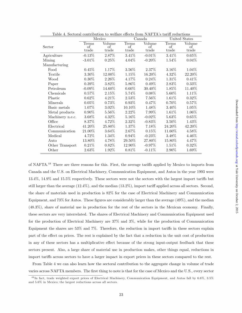
Table 4. Sectoral contribution to welfare effects from NAFTA’s tariff reductionsMexico Canada United States

SectorTermsoftrade

Volumeoftrade

Termsoftrade

Volumeoftrade

Termsoftrade

Volumeoftrade

Agriculture -0.13% 2.87% 3.41% -0.01% 3.41% 0.65%Mining -3.01% 0.25% 4.04% -0.20% 1.54% 0.04%ManufacturingFood 0.45% 1.17% 3.56% 2.37% 3.16% 1.04%Textile 3.30% 12.00% 1.15% 16.20% 4.32% 22.20%Wood 0.30% 2.26% 4.17% 0.24% 1.31% 0.41%Paper 0.39% 3.82% 5.86% 0.49% 2.83% 0.33%Petroleum -0.09% 14.60% 0.60% 30.40% 1.85% 11.40%Chemicals 0.57% 2.15% 5.74% 0.08% 5.60% 1.11%Plastic 0.62% 4.21% 2.53% 7.56% 1.61% 0.32%Minerals 0.05% 0.73% 0.93% 0.47% 0.70% 0.57%Basic metals 1.07% 3.02% 10.10% 1.48% 3.40% 1.05%Metal products 0.90% 5.56% 2.22% 7.99% 1.61% 1.06%Machinery n.e.c. 3.68% 4.32% 5.16% -0.02% 5.63% 0.65%Offi ce 8.37% 4.72% 2.32% -0.83% 3.50% 1.43%Electrical 41.20% 25.80% 1.37% 7.18% 24.20% 42.20%Communication 21.00% 3.64% 2.67% 0.15% 11.60% 4.58%Medical 4.72% 1.34% 0.94% -0.23% 3.48% 4.46%Auto 13.80% 4.78% 29.50% 27.80% 15.80% 4.47%Other Transport 0.21% 0.82% 12.90% -0.97% 1.51% 0.32%Other 2.63% 1.92% 0.81% -0.11% 2.90% 1.69%

of NAFTA.48 There are three reasons for this. First, the average tariffs applied by Mexico to imports from

Canada and the U.S. on Electrical Machinery, Communication Equipment, and Autos in the year 1993 were

13.4%, 14.9% and 15.5% respectively. These sectors were not the sectors with the largest import tariffs but

still larger than the average (12.4%), and the median (13.2%), import tariff applied across all sectors. Second,

the share of materials used in production is 82% for the case of Electrical Machinery and Communication

Equipment, and 73% for Autos. These figures are considerably larger than the average (49%), and the median

(48.3%), share of material use in production for the rest of the sectors in the Mexican economy. Finally,

these sectors are very interrelated. The shares of Electrical Machinery and Communication Equipment used

for the production of Electrical Machinery are 37% and 3%, while for the production of Communication

Equipment the shares are 53% and 7%. Therefore, the reduction in import tariffs in these sectors explain

part of the effect on prices. The rest is explained by the fact that a reduction in the unit cost of production

in any of these sectors has a multiplicative effect because of the strong input-output feedback that these

sectors present. Also, a large share of material use in production makes, other things equal, reductions in

import tariffs across sectors to have a larger impact in export prices in these sectors compared to the rest.

From Table 4 we can also learn how the sectoral contribution to the aggregate change in volume of trade

varies across NAFTAmembers. The first thing to note is that for the case of Mexico and the U.S., every sector

48 In fact, trade weighted export prices of Electrical Machinery, Communication Equipment, and Autos fall by 6.6%, 3.5%and 5.6% in Mexico; the largest reductions across all sectors.

23

at Yale U



ownloaded from


has a positive contribution to the welfare increase from volume of trade. Three sectors account for more than

50% of the sectoral contribution of Mexico’s and U.S.’s volume of trade. These are Textiles, Petroleum and

Electrical Machinery. For the case of Canada, the sectors that contribute the most are Textiles, Petroleum

and Auto. In general, volume of trade effects depend on the magnitude of the tariff reduction, the trade

elasticity, and the share of materials used in production and these factors weight differently for each of these

sectors. Textiles was the most protected sector by Mexico in the year 1993. Applied import tariffs were

on average 18%. So the large reduction in tariffs facilitates trade between members of NAFTA and results

in a significant contribution to the increase in volume of trade. Petroleum is a homogenous good sector.

As a consequence, small changes in import tariffs can have large trade effects since it is relatively easy to

substitute suppliers, as documented by its high import tariff trade elasticity (see Table 1). The average

import tariffs in Petroleum in the year 1993 across NAFTA members was 7%. Finally, NAFTA’s tariffs

reductions has important effects over the price of intermediate goods traded in some sectors compared to

others. This is particularly important for the sectors Electrical Machinery and Autos for reasons we discussed

in the previous paragraph. The reduction in trade prices in these sectors explains the increase in the volume

of trade effect.

Table 5. Trade effects from NAFTA’s tariff reductionsMexico Canada U.S.

Mexico’s imports - 116.60% 118.31%Canada’s imports 58.57% - 9.49%U.S.’s imports 109.54% 6.57% -

Table 5 presents aggregate trade effects from NAFTA. As we can see, NAFTA generated large aggregate

trade effects for all members. Mexico’s imports from NAFTA increased by more than 110% and equally so

across both partners. For the case of Canada, we find that the percentage increase in imports from Mexico

is more than five times larger than the percentage increase in imports from the U.S. This results reflect

that Mexico’s role as a supplier of intermediate goods to NAFTA members increased as a consequence of

NAFTA. In fact, this is even more evident when we look at the case of the U.S. imports. Imports from

Mexico increase more than 100% while from Canada only 6.57%. These figures reflect how interdependent

these economies become after the tariff reductions imposed by the agreement. In short, NAFTA strengthened

the trade dependence that these countries had before the agreement, and as a consequence Canada and the

U.S. source more goods from Mexico, while Mexico sources more goods from Canada and the U.S.

NAFTA also had an effect on sectoral specialization. Table 6 presents export shares by industry before

and after reducing NAFTA’s tariffs. First note that sectoral concentration varies considerably across sectors

and countries. Consider the case of Mexico before NAFTA, the year 1993. Three sectors account for 52.75%

of total exports. These sectors are Electrical Machinery, Autos and Mining. For the case of Canada, the

three sectors with the largest shares are Autos, Basic Metals and Mining, and account for 43.7% of total

exports. While for the U.S. the three largest sectors are Machinery, Chemicals, and Autos, and account for

24

at Yale U



ownloaded from


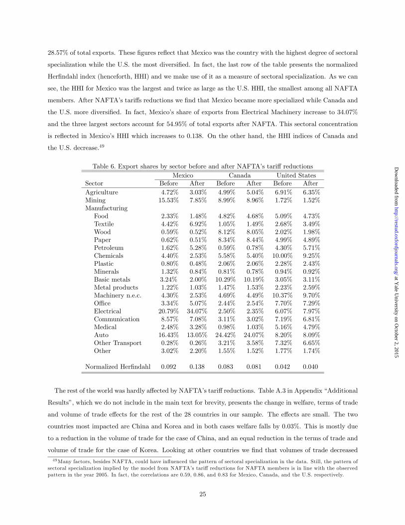
28.57% of total exports. These figures reflect that Mexico was the country with the highest degree of sectoral

specialization while the U.S. the most diversified. In fact, the last row of the table presents the normalized

Herfindahl index (henceforth, HHI) and we make use of it as a measure of sectoral specialization. As we can

see, the HHI for Mexico was the largest and twice as large as the U.S. HHI, the smallest among all NAFTA

members. After NAFTA’s tariffs reductions we find that Mexico became more specialized while Canada and

the U.S. more diversified. In fact, Mexico’s share of exports from Electrical Machinery increase to 34.07%

and the three largest sectors account for 54.95% of total exports after NAFTA. This sectoral concentration

is reflected in Mexico’s HHI which increases to 0.138. On the other hand, the HHI indices of Canada and

the U.S. decrease.49

Table 6. Export shares by sector before and after NAFTA’s tariff reductionsMexico Canada United States

Sector Before After Before After Before AfterAgriculture 4.72% 3.03% 4.99% 5.04% 6.91% 6.35%Mining 15.53% 7.85% 8.99% 8.96% 1.72% 1.52%ManufacturingFood 2.33% 1.48% 4.82% 4.68% 5.09% 4.73%Textile 4.42% 6.92% 1.05% 1.49% 2.68% 3.49%Wood 0.59% 0.52% 8.12% 8.05% 2.02% 1.98%Paper 0.62% 0.51% 8.34% 8.44% 4.99% 4.89%Petroleum 1.62% 5.28% 0.59% 0.78% 4.30% 5.71%Chemicals 4.40% 2.53% 5.58% 5.40% 10.00% 9.25%Plastic 0.80% 0.48% 2.06% 2.06% 2.28% 2.43%Minerals 1.32% 0.84% 0.81% 0.78% 0.94% 0.92%Basic metals 3.24% 2.00% 10.29% 10.19% 3.05% 3.11%Metal products 1.22% 1.03% 1.47% 1.53% 2.23% 2.59%Machinery n.e.c. 4.30% 2.53% 4.69% 4.49% 10.37% 9.70%Offi ce 3.34% 5.07% 2.44% 2.54% 7.70% 7.29%Electrical 20.79% 34.07% 2.50% 2.35% 6.07% 7.97%Communication 8.57% 7.08% 3.11% 3.02% 7.19% 6.81%Medical 2.48% 3.28% 0.98% 1.03% 5.16% 4.79%Auto 16.43% 13.05% 24.42% 24.07% 8.20% 8.09%Other Transport 0.28% 0.26% 3.21% 3.58% 7.32% 6.65%Other 3.02% 2.20% 1.55% 1.52% 1.77% 1.74%

Normalized Herfindahl 0.092 0.138 0.083 0.081 0.042 0.040

The rest of the world was hardly affected by NAFTA’s tariff reductions. Table A.3 in Appendix “Additional

Results”, which we do not include in the main text for brevity, presents the change in welfare, terms of trade

and volume of trade effects for the rest of the 28 countries in our sample. The effects are small. The two

countries most impacted are China and Korea and in both cases welfare falls by 0.03%. This is mostly due

to a reduction in the volume of trade for the case of China, and an equal reduction in the terms of trade and

volume of trade for the case of Korea. Looking at other countries we find that volumes of trade decreased49Many factors, besides NAFTA, could have influenced the pattern of sectoral specialization in the data. Still, the pattern of

sectoral specialization implied by the model from NAFTA’s tariff reductions for NAFTA members is in line with the observedpattern in the year 2005. In fact, the correlations are 0.59, 0.86, and 0.83 for Mexico, Canada, and the U.S. respectively.

25

at Yale U



ownloaded from


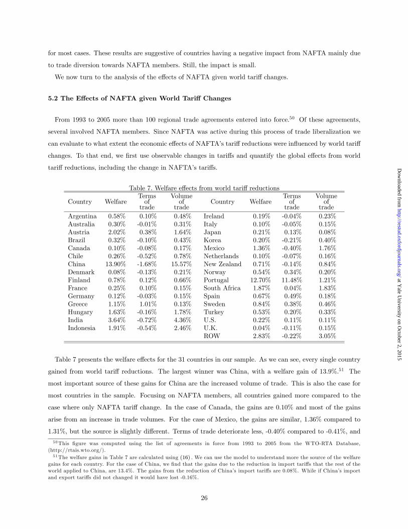
for most cases. These results are suggestive of countries having a negative impact from NAFTA mainly due

to trade diversion towards NAFTA members. Still, the impact is small.

We now turn to the analysis of the effects of NAFTA given world tariff changes.

5.2 The Effects of NAFTA given World Tariff Changes

From 1993 to 2005 more than 100 regional trade agreements entered into force.50 Of these agreements,

several involved NAFTA members. Since NAFTA was active during this process of trade liberalization we

can evaluate to what extent the economic effects of NAFTA’s tariff reductions were influenced by world tariff

changes. To that end, we first use observable changes in tariffs and quantify the global effects from world

tariff reductions, including the change in NAFTA’s tariffs.

Table 7. Welfare effects from world tariff reductions

Country WelfareTermsoftrade

Volumeoftrade


Volumeoftrade

Argentina 0.58% 0.10% 0.48% Ireland 0.19% -0.04% 0.23%Australia 0.30% -0.01% 0.31% Italy 0.10% -0.05% 0.15%Austria 2.02% 0.38% 1.64% Japan 0.21% 0.13% 0.08%Brazil 0.32% -0.10% 0.43% Korea 0.20% -0.21% 0.40%Canada 0.10% -0.08% 0.17% Mexico 1.36% -0.40% 1.76%Chile 0.26% -0.52% 0.78% Netherlands 0.10% -0.07% 0.16%China 13.90% -1.68% 15.57% New Zealand 0.71% -0.14% 0.84%Denmark 0.08% -0.13% 0.21% Norway 0.54% 0.34% 0.20%Finland 0.78% 0.12% 0.66% Portugal 12.70% 11.48% 1.21%France 0.25% 0.10% 0.15% South Africa 1.87% 0.04% 1.83%Germany 0.12% -0.03% 0.15% Spain 0.67% 0.49% 0.18%Greece 1.15% 1.01% 0.13% Sweden 0.84% 0.38% 0.46%Hungary 1.63% -0.16% 1.78% Turkey 0.53% 0.20% 0.33%India 3.64% -0.72% 4.36% U.S. 0.22% 0.11% 0.11%Indonesia 1.91% -0.54% 2.46% U.K. 0.04% -0.11% 0.15%

ROW 2.83% -0.22% 3.05%

Table 7 presents the welfare effects for the 31 countries in our sample. As we can see, every single country

gained from world tariff reductions. The largest winner was China, with a welfare gain of 13.9%.51 The

most important source of these gains for China are the increased volume of trade. This is also the case for

most countries in the sample. Focusing on NAFTA members, all countries gained more compared to the

case where only NAFTA tariff change. In the case of Canada, the gains are 0.10% and most of the gains

arise from an increase in trade volumes. For the case of Mexico, the gains are similar, 1.36% compared to

1.31%, but the source is slightly different. Terms of trade deteriorate less, -0.40% compared to -0.41%, and

50This figure was computed using the list of agreements in force from 1993 to 2005 from the WTO-RTA Database,(http://rtais.wto.org/).51The welfare gains in Table 7 are calculated using (16) . We can use the model to understand more the source of the welfare

gains for each country. For the case of China, we find that the gains due to the reduction in import tariffs that the rest of theworld applied to China, are 13.4%. The gains from the reduction of China’s import tariffs are 0.08%. While if China’s importand export tariffs did not changed it would have lost -0.16%.

26

at Yale U



ownloaded from


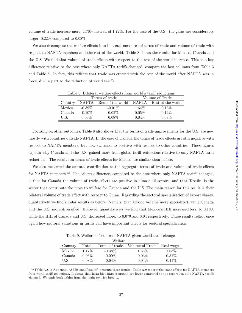
volume of trade increase more, 1.76% instead of 1.72%. For the case of the U.S., the gains are considerably

larger, 0.22% compared to 0.08%.

We also decompose the welfare effects into bilateral measures of terms of trade and volume of trade with

respect to NAFTA members and the rest of the world. Table 8 shows the results for Mexico, Canada and

the U.S. We find that volume of trade effects with respect to the rest of the world increase. This is a key

difference relative to the case where only NAFTA tariffs changed; compare the last columns from Table 3

and Table 8. In fact, this reflects that trade was created with the rest of the world after NAFTA was in

force, due in part to the reduction of world tariffs.

Table 8. Bilateral welfare effects from world’s tariff reductionsTerms of trade Volume of Trade

Country NAFTA Rest of the world NAFTA Rest of the worldMexico -0.39% -0.01% 1.64% 0.13%Canada -0.10% 0.02% 0.05% 0.12%U.S. 0.03% 0.08% 0.04% 0.08%

Focusing on other outcomes, Table 8 also shows that the terms of trade improvements for the U.S. are now

mostly with countries outside NAFTA. In the case of Canada the terms of trade effects are still negative with

respect to NAFTA members, but now switched to positive with respect to other countries. These figures

explain why Canada and the U.S. gained more from global tariff reductions relative to only NAFTA tariff

reductions. The results on terms of trade effects for Mexico are similar than before.

We also measured the sectoral contribution to the aggregate terms of trade and volume of trade effects

for NAFTA members.52 The salient difference, compared to the case where only NAFTA tariffs changed,

is that for Canada the volume of trade effects are positive in almost all sectors, and that Textiles is the

sector that contribute the most to welfare for Canada and the U.S. The main reason for this result is their

bilateral volume of trade effect with respect to China. Regarding the sectoral specialization of export shares,

qualitatively we find similar results as before. Namely, that Mexico became more specialized, while Canada

and the U.S. more diversified. However, quantitatively we find that Mexico’s HHI increased less, to 0.133,

while the HHI of Canada and U.S. decreased more, to 0.079 and 0.04 respectively. These results reflect once

again how sectoral variations in tariffs can have important effects for sectoral specialization.

Table 9. Welfare effects from NAFTA given world tariff changesWelfare


52Table A.8 in Appendix “Additional Results”presents these results. Table A.9 reports the trade effects for NAFTA membersfrom world tariff reductions. It shows that intra-bloc import growth are lower compared to the case when only NAFTA tariffschanged. We omit both tables from the main text for brevity.

27

at Yale U



ownloaded from


We now recalibrate the model to the year 1993 and introduce the observed change in world tariff structure

from 1993 to the year 2005 holding NAFTA tariffs fixed. In this way we measure the economic effects of all

observed world tariff changes excluding the reduction in NAFTA’s tariffs. After this, we compare the gains

from world tariff reductions with and without NAFTA. In other words, the effects of NAFTA given world

tariff changes. Table 9 presents the welfare effects. As we can see, welfare and real wage changes for Canada

and the U.S. are almost identical to the ones we find in the previous subsection, Table 2. For the case of

Mexico, the welfare effects and real wage effects are somehow smaller. The main reason for this lower gains

is that volume of trade effects are lower, 1.55% instead of 1.80%.

Table 10. Bilateral welfare effects from NAFTA given world tariff changesTerms of trade Volume of Trade

Country NAFTA Rest of the world NAFTA Rest of the worldMexico -0.37% -0.01% 1.78% -0.23%Canada -0.08% -0.01% 0.08% -0.05%U.S. 0.03% 0.01% 0.04% 0.00%

As we did before, we can make use of the bilateral measure of terms of trade to identify the reason why

Mexico’s volume of trade effects fall. We find that this is a consequence of the reduction in volume of

trade effects with respect to the rest of the world, not with respect to NAFTA members. Table 10 presents

these results. As we can see, Mexico’s volume of trade effects fall by 0.23% with the rest of the world.

Therefore, we find a larger negative effect due to trade diversion compared to the case when only NAFTA’s

tariff changed, last column of Table 3. The logic of this result is as follows. When we evaluate the effects of

NAFTA holding world tariffs fixed, trade is diverted from the lowest cost supplier outside NAFTA to a new

lower cost supplier inside the bloc, because of the lower tariffs. Now, as we also allow tariffs with respect to

the rest of the world to change, there is a larger pool of lowest cost suppliers in the world that Mexico is not

getting access to, because of low NAFTA tariffs. In this sense, what the model is measuring is the implied

trade diversion from NAFTA. Said differently, the change in world tariffs has raised the opportunity cost,

measured by the volume of trade effect, of belonging to NAFTA.53

5.3 The Effects of NAFTA Across Different Models

We now quantify the role that different mechanisms in our model have at explaining the results. We

compare the results from our model (Benchmark) to a one sector model (One sector), a multi sector model

53Tables A.10 to A.13 in Appendix “Additional Results” presents additional welfare and trade effects at the aggregate andsectoral level. Overall, we find that the results are similar to the case when only NAFTA’s tariff change, Section 5.1. We alsoperformed an additional counterfactual exercise to quantify how the welfare gains from NAFTA compare to a unilateral tariffelimination by each member. We do this exercise calibrating the model to the year 1993 and then, for each NAFTA memberindependently, we reduce their import tariffs to zero with respect to every country in the world. As a result, we find a welfareincrease of 0.54% for Mexico and a welfare loss of 0.03% and 0.02% for Canada and the U.S. respectively. Real wage increase by1.53%, 0.60% and 0.19%, for Mexico, Canada and the U.S. These welfare effects are due to the standard optimal tariff reasons.

28

at Yale U



ownloaded from


with no materials used in production (No materials), and with no I-O connections (No I-O).54 We calibrate

each of these models to the year 1993 and compute the welfare and trade responses from NAFTA’s tariff

reductions. Table 11 presents the simulated trade and welfare effects implied by the different models. The

first column shows the welfare effect from the one sector model. The second column presents the welfare

result for the no materials model, and the third column presents the welfare result for the no I-O model.

Table 11. Trade and welfare effects from NAFTA across different modelsWelfare Imports growth from NAFTA members

Multi sector Multi sectorCountry One sector No materials No I-O One sector No materials No I-O BenchmarkMexico 0.41% 0.50% 0.66% 60.99% 88.08% 98.96% 118.28%Canada -0.08% -0.03% -0.04% 5.98% 9.95% 10.14% 11.11%U.S. 0.05% 0.03% 0.04% 17.34% 26.91% 30.70% 40.52%

We find that for all models the welfare effects are smaller compared to the benchmark model. Still, in

all cases Mexico gains the most followed by the U.S. then Canada. The results from the one sector model

reflect the importance of accounting for sectoral heterogeneity. In fact, recent studies have emphasized

that the sectoral variation in trade elasticities is particularly important for the quantification of the welfare

gains.55 The calculations also show that intermediate goods amplify the welfare effects from tariff reductions.

Mexico’s figure increase from 0.50% to 0.66%, Canada’s deteriorate more from -0.03% to -0.04% and the

U.S. increase from 0.03% to 0.04% as we move from a model with no materials to a model with materials.

We also find that the model with input-output linkages amplifies the effects as well. If we compare the third

column on Table 11 to the results from the benchmark model, Table 2, we can clearly see that the welfare

effects are substantially larger for the countries that win and lower for the countries that loose.

Trade effects are also smaller across these models compared to the benchmark case. The last four columns of

Table 11 presents, for the case of Mexico, Canada and the U.S., the change in imports from NAFTA members

implied by the different models. As we can see, the trade effects are reduced substantially compared to the

benchmark case. In the one sector model, the trade responses are almost reduced by half. The intuition for

this result relates to the result on welfare. By averaging out the effects, a one sector model fails to capture

the large increase in trade flows from certain sectors. In fact, we know from tables 4 and 6 that NAFTA

generated very heterogenous responses across sectors. If we compare the results from column five to column

six we can see that adding intermediate goods increases the trade effects. The intuition for this result is

54The one sector model has one tradable sector and one non-tradable sector. Production uses materials from both sectors,(I-O). We agregate all sectoral data to calibrate the parameters and use the median tariff across sectors. We use our specification(23) to estimate an aggregate elasticity, the value is θ = 4.5. In the multi-sector model “No materials” there are no materialsused in production, γjn = 1, and as a result value added is equal to gross output. In the multi sector model “No I-O”, materialsare used in production, γjn < 1, but we zero out the off-diagonal elements of the I-O matrix. Firms can only use materialssourced from the same sector they operate, γj,jn = 1 − γjn. We use I-O tables for each country to calibrate γj,jn . For all cases,we first calibrate the model and then eliminate the observed aggregate trade deficits.55 In a recent study, Ossa (2012) shows that the heterogeneity in trade elasticities per se has an important effect on the

quantification of the welfare gains from trade. He shows this for the case of iceberg trade costs and by calculating welfare lossesfrom reverting to autarky.

29

at Yale U



ownloaded from


as follows. In the model with no materials, goods are only traded to produce final goods for consumption

and not for the production of intermediate goods. However, in the no I-O model, materials are also used for

the production of intermediate goods. Therefore, a tariff reduction delivers a larger trade effect due to the

increase in demand of tradable goods for the production of intermediates. Finally, we can also compare the

implied changes in trade flows from a model with intermediate goods in production but no sectoral linkages,

the no I-O model, to the benchmark case. The trade effects from tariff reductions are lower in the no I-O

model than in the model with sectoral interrelations (Benchmark). The reason is that since producers are

only using inputs from one sector they are not exploiting the benefits of having access to cheaper materials

from other sectors. This in turn delivers a smaller trade effect from tariff changes. In short, the results

from this subsection unmask the importance of accounting for sectoral heterogeneity, intermediate goods in

production and I-O linkages to evaluate the trade and welfare gains from tariff changes, in general, and in

particular for the case of NAFTA.

6. CONCLUSION

This study develops a general equilibrium model to quantify the trade and welfare effects of tariff changes.

The model is able to perform complex trade policy evaluations for an arbitrary number of sectors and

countries in a parsimonious way with few data and parameter requirements. Using the model we decompose

the different channels by which a reduction in tariffs can spread the gains across sectors in the economy.

We show that accounting for sectoral interrelations is quantitatively and economically meaningful. With the

model, one can quantify and decompose the effects that a reduction or increase in a tariff in a particular

sector can have on the price of intermediate inputs in that sector and in the rest of the economy, the general

equilibrium price effects of tariff reductions at home and abroad, the impact on factor allocations across

sectors, the change in factor payments and the extent to which the structure of production of a particular

economy can spread the gains from having access to cheaper intermediate goods and more effi cient technology.

Evaluating the effects of NAFTA has receive considerable attention in the economic literature. Therefore,

it is important to clarify how our results about NAFTA should be interpreted. We use the model to perform

a model-based identification of the effects of NAFTA’s tariff reductions. Unquestionably, NAFTA had more

provisions than only reducing tariff between members and by no means our results should be interpreted as

the trade and welfare effects of the entire agreement. For instance, non-tariff barriers or unobservable trade

costs might also have changed as a consequence of NAFTA. Moreover, NAFTA might have even influenced

the rate of technological change of each member. Certainly, we could have used the model to quantify

what is the implied change in fundamental TFP and trade costs such that the model matches the trade

patterns observed in the data. However, understanding how fundamental TFP changed as a consequence of

NAFTA is outside of the scope of this paper. In our model fundamental TFP is exogenous and by holding

it fixed during the period of analysis we are able to identify the pure direct effect of tariff reductions. Our

30

at Yale U



ownloaded from


study uses the case of NAFTA to show how the effects of tariff reductions are amplified as we take into

account the interrelation across sectors observed in the data. We find that the trade and welfare effects from

tariff reductions are lower if intermediate goods in production and input-output linkages are ignored in the

analysis. With this results we hope to convey the message that modelling sectoral interrelations is not only

feasible but also important for quantitative analysis.

31

at Yale U



ownloaded from


REFERENCES

[1] Alvarez, Fernando, and Robert E. Lucas (2007): “General Equilibrium Analysis of the Eaton-Kortum Modelof International Trade,”Journal of Monetary Economics, 54(6), 726—68.

[2] Anderson, James E. (1979): “A Theoretical Foundation for the Gravity Equation,”American EconomicReview, 69(1), 106-116.

[3] Anderson, Michael A., Edward J. Balistreri, Alan Fox, and Russell H. Hillberry (2005): “Taste Parameters asModel Residuals: Assessing the Fit of an Armington Trade Model,”Review of International Economics,13(5), 973-984.

[4] Anderson, James E., and Douglas Marcouiller (2002): “Insecurity and the Pattern of Trade: An EmpiricalInvestigation,”Review of Economics and Statistics, 84(2), 342-352.

[5] Anderson, James E., and Eric van Wincoop (2002): “Borders, Trade and Welfare”, in S. Collins and D.Rodrik eds, Brookings Trade Policy Forum 2001, 207—230.

[6] Anderson, James E., and Eric van Wincoop (2003): “Gravity with Gravitas: A Solution to the BorderPuzzle,”American Economic Review, 93(1), 170-192.

[7] Anderson, James E., and Eric van Wincoop (2004): “Trade Costs,”Journal of Economic Literature, 42(3),691-751.

[8] Arkolakis, Costas, Arnaud Costinot, and Andres Rodriguez Clare (2012): “New Theories, Same Old Gains?,”American Economic Review, 102(1), 94-130.

[9] Armington, Paul (1969): “A Theory of Demand for Products Distinguished by Place of Production,” IMFStaff Papers, 16(1), 159-176.

[10] Bagwell, Kyle, and Robert Staiger (1999): “An Economic Theory of GATT,”American Economic Review,89(1), 215-248.

[11] Bagwell, Kyle, and Robert Staiger (2010): “The World Trade Organization: Theory and Practice,”AnnualReview of Economics, 2(1), 223-256.

[12] Baier, Scott, and Jeffrey Bergstrand (2007): “Do Free Trade Agreements Actually Increase Members’Inter-national Trade?,”Journal of International Economics 71(1), 72-95.

[13] Baier, Scott, and Jeffrey Bergstrand (2009): “Estimating the Effects of Free Trade Agreements on TradeFlows using Matching Econometrics,”Journal of International Economics, 77(1), 77-85.

[14] Baldwin, Richard E., and Antony J. Venables (1995): “Regional Economic Integration,” in Handbook ofInternational Economics (G. M. Grossman and K. Rogoff eds.), vol. 3: 1597-1644, North-Holland,Amsterdam.

[15] Bergstrand, Jeffrey H., Peter Egger, and Mario Larch (2013): “Gravity Redux: Estimation of Gravity-Equation Coeffi cients, Elasticities of Substitution, and General Equilibrium Comparative Statics underAsymmetric Bilateral Trade Costs,”Journal of International Economics, 89(1), 110-121.

[16] Bhagwati, Jagdish, Pravin Krishna, and Arvind Panagariya (eds.) (1999): “Trading Blocs: AlternativeApproaches to Analyzing Preferential Trade Agreements,”MIT Press, Cambridge, Massachusetts.

[17] Bishop, Jesse (2006): “Substitution Elasticities and the Cost of Protection: Evidence from the 2002 U.S.Steel Tariffs,”unpublished working paper, University of Minnesota.

[18] Broda, Christian, and David Weinstein (2006): “Globalization and the Gains from Variety,” QuarterlyJournal of Economics, 121(2), 541-585.

[19] Brown, Drusilla K., Alan V. Deardorff, and Robert M. Stern (1994): “Estimates of a North American FreeTrade Agreement,”unpublished working paper, Federal Reserve Bank of Minneapolis.

32

at Yale U



ownloaded from


[20] Brown, Drusilla K., and Robert M. Stern (1989): “U.S.-Canada Bilateral Tariff Elimination: The Role ofProduct Differentiation and Market Structure,”in Trade policies for International Competitiveness, ed.Robert C. Feenstra, pp. 217—45. Chicago: University of Chicago Press.

[21] Burstein, Ariel, and Jonathan Vogel (2012): “International Trade, Technology, and the Skill Premium,”unpublished working paper, Columbia University.

[22] Burstein, Ariel, Javier Cravino, and Jonathan Vogel (2013): “Importing Skill-Biased Technology,”AmericanEconomic Journal: Macroeconomics, 5(2), 32-71.

[23] Caliendo, Lorenzo, and Fernando Parro (2010): “Welfare Gains from Changing Partners in a Trade Bloc:The Case of MERCOSUR,” in Hamid Beladi, E. Kwan Choi (ed.) New Developments in ComputableGeneral Equilibrium Analysis for Trade Policy (Frontiers of Economics and Globalization, Volume 7),Emerald Group Publishing Limited, pp.41-60.

[24] Campa, Jose Manuel, and Linda S. Goldberg (1997): “The Evolving External Orientation of ManufacturingIndustries: Evidence from Four Countries,”Federal Reserve Bank of New York Economic Policy Review,3(2), 53-81.

[25] Caselli, Francesco, Miklos Koren, Milan Lisicky, and Silvana Tenreyro (2012): “Diversification throughTrade,”mimeo LSE.

[26] Chaney, Thomas (2008): “Distorted Gravity: The Intensive and Extensive Margins of International Trade,”American Economic Review, 98(4), 1707-1721.

[27] Chor, Davin (2010): “Unpacking Sources of Comparative Advantage: A Quantitative Approach,”Journalof International Economics, 82(2), 152-167.

[28] Clausing, Kimberly A. (2001): “Trade Creation and Trade Diversion in the Canada-United States Free TradeAgreement,”Canadian Journal of Economics, 34(3), 677-696.

[29] Costinot, Arnaud, Dave Donaldson, and Ivana Komunjer (2012): “What Goods Do Countries Trade? AQuantitative Exploration of Ricardo’s Ideas?,”Review of Economic Studies, 79(2), 581-608.

[30] Deardorff, Alan V. (1998): “Determinants of Bilateral Trade: Does Gravity Work in a Neoclassical World?,”in Jeffrey A. Frankel, ed., The Regionalization of the World Economy. University of Chicago Press.

[31] Dekle, Robert, Jonathan Eaton, and Samuel S. Kortum (2008): “Global Rebalancing with Gravity: Mea-suring the Burden of Adjustment,”IMF Staff Papers, 55(3), 511-540.

[32] Dixit, A. and V. Norman, (1980): “The Theory of International Trade: A Dual General Equilibrium Ap-proach,”Cambridge University Press.

[33] Dixit, Arvind.K., and Joseph E. Stiglitz (1977): “Monopolistic Competition and Optimum Product Diver-sity,”American Economic Review, 67(3), 297-308.

[34] Donaldson, Dave (2012): “Railroads of the Raj: Estimating the Impact of Transportation Infrastructure,”American Economic Review, forthcoming.

[35] Eaton, Jonathan, and Samuel S. Kortum (2002): “Technology, Geography, and Trade,”Econometrica, 70(5),1741—1779.

[36] Eaton, Jonathan, and Samuel S. Kortum (2012): “Putting Ricardo to Work,”Journal of Economic Perspec-tives, 26(2): 65—90.

[37] Eaton, Jonathan, Sam Kortum, Brent Neiman, and John Romalis (2011): “Trade and the Global Recession”,NBER Working Paper No 16666.

[38] Ethier, Wilfred J. (1982): “National and International Returns to Scale in the Theory of InternationalTrade,”American Economic Review, 72(3), 389-405.

[39] Feenstra, Robert C. 1994. “New Product Varieties and the Measurement of International Prices,”AmericanEconomic Review, 84(1), 137-77.

33

at Yale U



ownloaded from


[40] Feenstra, Robert C., and Gordon Hanson (1996): “Globalization, Outsourcing and Wage Inequality,”Amer-ican Economic Review 86(2), 240-245.

[41] Fieler, Cecilia (2011): “Non-Homotheticity and Bilateral Trade: Evidence and a Quantitative Explanation,”Econometrica, 79(4), 1069-1101.

[42] Fox, Alan K. (1999): “Evaluating the Success of a CGE Model of the Canada-U.S. Free Trade Agreement,”unpublished working paper, Michigan University.

[43] Hallak, Juan Carlos (2006): “Product Quality and the Direction of Trade,” Journal of International Eco-nomics, 68(1), 238-265.

[44] Head, Keith, and Thierry Mayer (2001): “Illusory Border Effects: Distance Mismeasurement Inflates Esti-mates of Home Bias in Trade,”CEPII Working Papers 2002-01.

[45] Head, Keith, Thierry Mayer, and John Ries (2009): “The Erosion of Colonial Trade Linkages After Inde-pendence,”CEPR Discussion Paper No 6951.

[46] Head, Keith, and John Ries (2001): “Increasing Returns versus National Product Differentiation as anExplanation for the Pattern of U.S.-Canada Trade,”American Economic Review, 91(4), 858-876.

[47] Hertel, Thomas.W., David Hummels, Maros Ivanic, and Roman Keeney (2003): “How Confident Can WeBe in CGE-Based Assessments of Free Trade Agreements,”GTAP Working Paper No. 26.

[48] Hsieh, Chang-Tai, and Ralph Ossa (2011): “A Global View of Productivity Growth in China,” NBERworking paper No 16778.

[49] Hummels, David, Jun Ishii, and Kei-Mu Yi (2001): “The Nature and Growth of Vertical Specialization inWorld Trade,”Journal of International Economics, 54(1), 75-96.

[50] Imbs, Jean, and Isabelle Méjean (2011): “Elasticity Optimism,”CEPR Discussion Paper No 7177.

[51] Jones, Charles I. (2007): “The Input-Output Multiplier and Economic Development,”unpublished workingpaper, U.C. Berkeley.

[52] Kehoe, Timothy J. (2003): “An Evaluation of the Performance of Applied General Equilibrium Models ofthe Impact of NAFTA,”Federal Reserve Bank of Minneapolis Working Paper No. 320.

[53] Kehoe, Patrick, and Timothy J. Kehoe (1994): “Capturing NAFTA’s Impact with Applied General Equilib-rium Models,”Federal Reserve Bank of Minneapolis Quarterly Review, 18(2), 17-34.

[54] Kerr, William R. (2009): “Heterogeneous Technology Diffusion and Ricardian Trade Patterns,”unpublishedworking paper, Harvard Business School.

[55] Krueger, Anne O. (1999): “Trade Creation and Trade Diversion Under NAFTA,”NBER Working Paper No7429.

[56] Krugman, Paul, (1981): “Intraindustry specialization and the Gains from Trade,”Journal of Political Econ-omy, 86(5), 959-973.

[57] Krugman, Paul (1991): “Increasing Returns and Economic Geography,”Journal of Political Economy, 99(3),483-99.

[58] Lederman, Daniel, William F. Maloney, and Luis Servén (2005): “Lessons from NAFTA for Latin Americaand the Caribbean,” Stanford University Press and the World Bank, Latin American DevelopmentForum Series: Palo Alto, California and Washington, DC.

[59] Levchenko, Andrei, and Jing Zhang (2011): “The Evolution of Comparative Advantage: Measurement andWelfare Implications,”NBER Working Paper No 16806.

[60] Martin, Philippe, Thierry Mayer, and Mathias Thoenig (2008): “Make Trade NotWar?,”Review of EconomicStudies, 75(3), 865—900.

34

at Yale U



ownloaded from


[61] Melitz, Marc J. (2003): “The Impact of Trade on Intra-industry Reallocations and Aggregate IndustryProductivity,”Econometrica, 71(6), 1695-1725.

[62] Ossa, Ralph (2012): “Why Trade Matters After All,”NBER working paper No 18113.

[63] Ossa, Ralph (2014): “Trade Wars and Trade Talks with Data,”American Economic Review, forthcoming.

[64] Parro, Fernando (2013): “Capital-Skill Complementarity and the Skill Premium in a Quantitative Model ofTrade,”American Economic Journal: Macroeconomics, 5(2), 72-117.

[65] Ramondo, Natalia, and Andres Rodriguez-Clare (2013): “Trade, Multinational Production, and the Gainsfrom Openness,”Journal of Political Economy, 121(2), 273-322.

[66] Redding, Stephen, and Anthony J. Venables (2004): “Economic Geography and International Inequality,”Journal of International Economics, 62(1), 53-82.

[67] Rolleigh, Michael M. (2008): “Plant Heterogeneity and Applied General Equilibrium Models of Trade,”unpublished working paper, Williams College.

[68] Romalis, John (2007): “NAFTA’s and CUSTFA’s Impact on International Trade,”Review of Economicsand Statistics, 89(3), 416-435.

[69] Rose, Andrew K. (2004): “Do We Really Know That the WTO Increases Trade?,”American EconomicReview, 94 (1), 98-114.

[70] Samuelson, Paul (1954): “The Transfer Problem and Transport Costs, II: Analysis of Effects ofTrade.Impediments,”The Economic Journal, 64(2), 264-289.

[71] Shikher, Serge (2010): “Predicting the Effects of NAFTA: Now We Can Do It Better!,”Journal of Interna-tional and Global Economic Studies, forthcoming.

[72] Shikher, Serge (2011): “Capital, Technology, and Specialization in the Neoclassical Model,” Journal ofInternational Economics, 83(2), 229-242.

[73] Subramanian, Arvind, and Shang-Jin Wei (2007): “The WTO Promotes Trade, Strongly but Unevenly,”Journal of International Economics, 72(1), 151-75.

[74] Santos-Silva, J.M.C., and Silvana Tenreyro (2010): “Estimation of Ratio Models when the Ratio Can Take0/0 Values,”unpublished working paper, LSE.

[75] Simonovska, Ina, and Michael Waugh (2013): “The Elasticity of Trade: Estimates and Evidence,”Journalof International Economics, forthcoming.

[76] Trefler, Daniel (1993): “Trade Liberalization and the Theory of Endogenous Protection: An Economic Studyof U.S. Import Policy,”Journal of Political Economy 101(1),138-60.

[77] Trefler, Daniel (2006): “The Long and Short of the Canada-U.S. Free Trade Agreement,” STICERD -Economics of Industry Papers 41, Suntory and Toyota International Centres for Economics and RelatedDisciplines, LSE.

[78] United Nations Conference on Trade and Development (UNCTAD) (2005): “Methodologies, Classifications,Quantification and Development Impacts of Non-Tariff Barriers: Note by the UNCTAD Secretariat,”Document TD/B/COM.1/EM.27/2, June 23.

[79] Viner, Jacob (1950): “The Customs Union Issue,”New York: Carnegie endowment for International Peace.

[80] Waugh, Michael (2010): “International Trade and Income Differences,”American Economic Review, 100(5),2093-2124.

[81] World Bank (2005): “Global Economic Perspective,”Washington DC.

[82] Yeats, Alexander (2001): “Just How Big Is Global Production Sharing?,”in Fragmentation: New ProductionPatterns in the World Economy, S.W. Arndt and K. Henryk (eds.). Oxford University Press.

[83] Yi, Kei-Mu (2003): “Can Vertical Specialization Explain the Growth of World Trade?,”Journal of PoliticalEconomy, 111(1), 52-102.

35

at Yale U



ownloaded from


APPENDIX: DISTRIBUTION OF PRICES AND EXPENDITURE SHARES

The effi ciency of country n in producing an intermediate good ωj in sector j is the realization of a random

variable zji drawn for each ωj in each sector j from the distribution F jn (z) = e−λ

jnz−θj

. Therefore, the costof purchasing an intermediate good ωj from country i, where we abuse of notation and denote by pjni(z

ji ), is

the realization of the random variable pjni(zji ) = cjiκ

jni/z

ji . First note that p

jni(z

ji ) has a Fréchet distribution,

in particular

Pr[pjni ≤ p

]= 1− e−T

jnip

θj

, (24)

where T jni = λji (cjiκjni)−θj . Given this, the lowest price of an intermediate good ωj in country n, namely

pjn(ωj), has also a Fréchet distribution,

Pr[pjn ≤ p

]= 1−

∏N

i=1Pr[pjni ≥ p

], (25)

and using (24) we obtain

Pr[pjn ≤ p

]= 1− e−Φjnp

θj

, (26)

where Φjn =∑N

i=1T jni =

∑N

i=1λji (c

jiκjni)−θj . The object Φjn plays a critical role in our model. It’s a

suffi cient statistic of the states of technologies around the world, input costs, geographic barriers and tariffpolicies. In Eaton and Kortum (2002), this object is country specific, while in our model it is also sectorspecific. Note that Φjn is correlated across sectors since sectors are interrelated and the input costs arefunctions of prices from all sectors. The shares γk,jn will determine the extent of the correlation. Note thatin a non-tradable goods sector, since κjin =∞, Φjn = λjn(cjn)−θ

j

.

It is convenient to work with pjn(ωj)θj

. Note that since pjn(ωj) is Fréchet with shape parameter θj , thenpjn(ωj)θ

j

has an exponential distribution. To see this, define the function g (x) = xθj

and suppose that x hasa Fréchet distribution with location parameter Φjn and shape parameter θ

j . Let fx (x) denote the density

function of x, namely fx (x) = θjΦjnxθj−1e−Φjnx

θj

. It follows that the density function of y = g (x) is given

by fy (y) = fx(g−1 (y)

)|∂g−1(y)∂y |. Then since g−1 (y) = y

1

θj , and ∂g−1(y)∂y = 1

θjy

1

θj−1, the density function of

y is fy (y) = Φjne−Φjny, which is an exponential distribution with parameter Φjn. Given this result, the price

index is

(P jn)1−ηj =

∫Φjny

(1−ηj)/θje−yΦjndy,

which follows since we have just derived that y = pjn(ωj)θj

has probability density function, Φjne−Φjny. Now

consider the change of variables u = Φjny. Then (P jn)1−σj = (Φjn)−(1−σj)/θj ∫ u(1−σj)/θje−udu, and finally

P jn = AjΦj −1/θj

n ,

which is the same as (4) , where Aj = Γ(ξj)1/(1−σj)

, and Γ(ξj)is a Gamma function evaluated at ξj =

1 +(1− σj

)/θj . For the case of a non-tradeable sector, Φjn = λjn(cjn)−θ

j

, and therefore P jn = Ajλjn(cjn)−θj

.

To derive the expenditure shares πjni = Xjni/X

jn, note that

Xjni = Pr

[cjiκ

jni

zji (ωj)≤ min

h6=i

cjhκjnh

zjh(ωj)

]Xjn.

Then using (24) , and (26) , note that

Xjni =

T jniΦjn

[∫ ∞0

Φjne−Φjnp

θj

θjp θj−1dp

]Xjn =

λji (cjiκjni)−θj∑N

i=1λji (c

jiκjni)−θj

Xjn,

and in this way obtain (6) .

36

at Yale U



ownloaded from


APPENDIX: WELFARE

We present a detailed derivation of the expression for the change in welfare, equation (16).

Welfare is given by Wn = wnLnPn

+ RnPn

+ DnPn, where recall that Rn =

∑Jj=1

∑Ni=1

τjniMjni

Pn. Totally differen-

tiating welfare and assuming that exogenous trade deficits remain constant, dDn = 0, and holding icebergtrade costs fixed, namely d lnκjni = d ln τ jni, we obtain

d lnWn =wnLnIn

d lnwn +RnInd lnRn − d lnPn. (27)

Now, totally differentiating tariff revenue we obtain

dRn =∑J

j=1

∑N

i=1τ jniM

jnid lnM j

ni +∑J

j=1Xjn

∑N

i=1πjnid ln τ jni. (28)

Totally differentiating the consumption price index (5) we obtain,

d lnPn =∑J

j=1αjnd ln pjn =

∑J

j=1αjn∑N

i=1πjni

(d ln cji + d ln τ jni

), (29)

where we use the definition of sectoral prices (4) , which then implies that d ln pjn =∑N

i=1πjni[d ln cji+d ln τ jni],

by (6) . Finally, from the definition of the input bundle (2) , we can obtain an expression for the change inwages. Totally differentiating this expression we get

d lnwn =1

γjnd ln cjn −

∑k=1

γk,jn

γjnd ln pkn. (30)

Substituting (28) , and (29) , into (27) we get

d lnWn =wnLnIn

d lnwn +1

In

∑J

j=1

∑N

i=1τ jniM

jnid lnM j

ni

+1

In

∑J

j=1Xjn

∑N

i=1πjnid ln τ jni

−∑J

j=1αjn∑N

i=1πjni

(d ln cji + d ln τ jni

),

using the intermediate goods market clearing condition (7) to solve for αjn, we obtain

d lnWn =wnLnIn

d lnwn +1

In

∑J

j=1

∑N

i=1τ jniM

jnid lnM j

ni∑J

j=1

∑k=1

γj,knγkn

wnLkn

In

∑N

i=1πjni

(d ln τ jni + d ln cji

)−∑J

j=1

Xjn

In

∑N

i=1πjnid ln cji ,

adding and substracting 1In

∑Jj=1

∑N

i=1Ejnid ln cjn, we obtain

d lnWn =wnLnIn

d lnwn +1

In

∑J

j=1

∑N

i=1τ jniM

jni

(d lnM j

ni − d ln cji

)− 1

In

∑J

j=1

∑N

i=1Ejni

(d ln cjn −

∑k=1

γk,jn d ln pkn

)

+1

In

∑J

j=1

∑N

i=1

(Ejnid ln cjn −M

jnid ln cji

),

and finally we use (30) to obtain (16) .

37

at Yale U



ownloaded from


APPENDIX: SOLVING THE MODEL

We present a step by step description on how to solve the model. Consider a change in policy from τ tothe new policy τ ′, captured by κjni or a change in Dn to D′n.

• Step 1: Guess a vector of wages w = (w1, ..., wN )

• Step 2: Use equilibrium conditions (10) and (11) to solve for prices in each sector and each country,pjn (w) and input costs, cjn (w) consistent with the vector of wages w.

• Step 3: Use the information on πjni and θj together with the solutions to pjn (w) and cjn (w) from step

2 and solve for πj′ni (w) using (12).

• Step 4: Given πj′ni (w) from step 3, the new tariff vector τ ′, and data for γjn, γj,kn and αjn, solve for

total expenditure in each sector j and country n, Xj′n (w) consistent with the vector of wages w in the

following way. Note that from (13) , the total expenditure in the counterfactual scenario is given by

Xj′n =

∑J

k=1γj,kn

∑N

i=1

πk′

in (w)

1 + τk′in

Xk′i + αjn(wnwnLn +

∑J

j=1

∑N

i=1τ j′niM

j′ni (w) +D′n). (31)

Equation (31) is a system of J ×N equations in J ×N total expenditures. Notice that if τ ′ = τ , andD′n = Dn then w = 1 and Xj′

n (1) = Xn. It is convenient to re-write the system of equations in matrixform:

Ω (w) X = ∆ (w) ,

where X is the vector of expenditures for each sector and country and ∆ (w) is a vector containing theshares of each sector and country in final demand, value added and aggregate trade deficit by country.Concretely,

X =

X1′1...

XJ′1...

X1′n...

XJ′N

JN×1

; ∆ (w) =

α11 (w1w1L1 +D′1)

...αJ1 (w1w1L1 +D′1)

...α1N (wNwNLN +D′N )

...αJN (wNwNLN +D′N )

JN×1

.

The matrix Ω (w) is a square matrix of dimensions JN × JN. Ω (w) captures the general equilibriumeffects of how changes in tariffs from one sector and one country impact expenditure in all other sectorsof the economy and the world. Ω (w) is constructed by adding three square matrices, I, z(w) andH(w). The matrix I is the identity matrix with dimensions JN × JN . The square matrix z(w) isconstructed using the following vectors,

An =

α1n...αJn

J×1

, F ′n (w) =( (

1− F 1′

n (w))· · ·

(1− F J′n (w)

) )1×J

,

where F j′

n (w) =∑Ni=1

πj′ni(w)

1+τj′ni. Then the matrix z(w) is defined as

z(w) =

A1 ⊗ F ′1 (w) 0J×J · · · 0J×J 0J×J

0J×J A2 ⊗ F ′2 (w) · · ·...

...

0J×J 0J×J. . . 0J×J 0J×J

...... · · · AN−1 ⊗ F ′N−1 (w) 0J×J

0J×J 0J×J · · · 0J×J AN ⊗ F ′N (w)

JN×JN

.

38

at Yale U



ownloaded from


The square matrix H (w) is given by:

H (w) =

γ1,11 π1′1,1 (w) · · · γ1,J1 πJ′1,1 (w) · · · γ1,11 π1′N,1 (w) · · · γ1,J1 πJ′N,1 (w)...

......

......

......

γJ,11 π1′1,1 (w) · · · γJ,J1 πJ′1,1 (w) · · · γJ,11 π1′N,1 (w) · · · γJ,J1 πJ′N,1 (w)...

......

......

......

γ1,1N π1′1,N (w) · · · γ1,JN πJ′1,N (w) · · · γ1,1N π1′N,N (w) · · · γ1,JN πJ′N,N (w)...

......

......

......

γJ,1N π1′1,N (w) · · · γJ,JN πJ′1,N (w) · · · γJ,1N π1′N,N (w) · · · γJ,JN πJ′N,N (w)

JN×JN

,

where πk′

in (w) =πk′in(w)

1+τk′in

. Finally, Ω (w) = I −z(w)− H(w). The interactions presented in Ω (w) are

the key differences compared to a one-sector model and a multi-sector model without I-O linkages. Forexample, in the special case in which γj,jn = 1 − γjn, tariffs do not appear in Ω (w) and expendituresin each country can be solved independently of the expenditures from other countries. For the case inwhich there is only one sector, Ω (w) collapses to a scalar as in Alvarez and Lucas (2007) and Eatonand Kortum (2002). In a two-sector model without tariffs and exogenous sectoral deficit, as in Dekle,Eaton and Kortum (2008), Ω (w) depends only on technology and preference parameters, (γ, α). Wesolve for the vector X (w) by inverting the matrix Ω (w).

X (w) = Ω−1 (w) ∆ (w) .

Denote by Xj′

n (w) the entry j of the vector X (w) (the expenditure in sector j and country n). Thisexpression is crucial in order to solve for the general equilibrium, since it allows us to express all theequilibrium conditions as a function of one vector of unknowns, the vector of factor prices, w.

• Step 5: Substitute πj′in (w), X (w), τ ′, and D′n into (14) and obtain:

∑J

j=1

∑N

i=1

πj′ni (w)

1 + τ j′niXj′n (w)−D′n =

∑J

j=1

∑N

i=1

πj′in (w)

1 + τ j′inXj′i (w) . (32)

Notice that we have just reduced the system of equilibrium conditions (10 through 13) to a system ofN equations (one trade balance per country) and N unknowns (one wage per country).

• Step 6: Verify if (32) holds. If not, we adjust our guess of w and proceed to step 1 again untilequilibrium condition (32) is obtained.

APPENDIX: CES MODEL

In this appendix we develop a model that allows for different degrees of substitutability across inputs.Consider a double nested constant elasticity of substitution (CES) production function, with an outer nestbetween labor and materials and an inner CES aggregator of materials from all sectors. Concretely, theproduction function of intermediate goods ωj is given by

qjn(ωj) = zjn(ωj) [[

χjn] 1η[ljn(ωj)

] η−1η +

[1− χjn

] 1η[M jn(ωj)

] η−1η

] ηη−1

,

where materials and labor are combined with a CES function with elasticity of substitution equal to η andweights given to χjn varying by sector and country. M

jn

(ωj)is the total materials demanded in sector j by

producer ωj in country n. We also allowed for a varying degree of substitution where materials from sectork used to produce intermediate goods in sector j are combined with a CES function with elasticity equal toρ and weights equal to δk,jn that vary across sectors and countries where

∑Jk=1 δ

k,jn = 1,

M jn

(ωj)

=

[∑J

k=1

[δk,jn

] 1ρ [mk,jn (ωj)

] ρ−1ρ

] ρρ−1

.

39

at Yale U



ownloaded from


In terms of the characterization of the equilibrium, two equations have to be modified with a CES model.First, the cost of the bundle of inputs now adopts a nested CES functional form given by

cjn =[[χjn]

[wn]1−η

+[1− χjn

] [PM,jn

]1−η] 11−η

, (33)

where PM,jn is the price index of materials used in production, given by

PM,jn =

[∑J

k=1δk,jn

[P kn]1−ρ] 1

1−ρ

. (34)

Second, the input shares are not constant with a CES model, and therefore the equation for total expen-diture is given by

Xjn =

∑J

k=1ξj,kn

∑N

i=1Xki

πkin1 + τkin

+ αjnIn, (35)

where ξj,kn is the share of inputs from sector j in sector k gross output.Mapping this shares to our previous notation, this implies that

γk,jn ≡ ξk,jn =(1− χjn

) [PM,jn

cjn

]1−η

δk,jn

[P kn

PM,jn

]1−ρ

, and γjn ≡ χjn[wn

cjn

]1−η.

Equilibrium in relative changes

In relative changes, the cost of bundle of inputs (33) becomes:

cjn =

[ζl,jn [wn]

1−η+∑J

k=1ξk,jn

[PM,jn

]1−η] 11−η

, (36)

and the price index (34) becomes

PM,jn =

[∑J

k=1ξk,jn

]− 11−ρ[∑J

k=1ξk,jn

[P kn

]1−ρ] 11−ρ

(37)

where ζl,jn is the share of labor in sector j gross output.Total expenditure (35) in the counterfactual equilibrium is given by

Xj′n =

∑J

k=1ξj,k′n

∑N

i=1Xk′i

πk′in1 + τk′in

+ αjnI′n, (38)

with

ξj,k′n =

ζl,kn∑Jj=1 ξ

j,kn

[PM,kn

wn

]η−1

+ 1

−1 ∑J

h=1

ξh,kn

ξj,kn

[P kn

Phn

]ρ−1−1

Equations (36) , (37) , (38) , together with equations (12), and (13) describe the equilibrium in relativechanges in a CES model.

40

at Yale U



ownloaded from


APPENDIX: DATA SOURCES AND DESCRIPTION

This appendix describes the data sources and data construction we use in the paper. The list of countriesincluded in our database is: Argentina, Australia, Austria, Brazil, Canada, Chile, China, Denmark, Finland,France, Germany, Greece, Hungary, India, Indonesia, Ireland, Italy, Japan, Korea, Mexico, Netherlands,New Zealand, Norway, Portugal, South Africa, Spain, Sweden, Turkey, UK, USA, and a constructed rest ofthe world. The list of sectors is reported in Table A.1.

Bilateral Trade Flows We use bilateral trade flows for the 20 tradable sectors described in TableA.1 and our sample of 31 countries for the year 1993. Bilateral trade data come from the United NationsStatistical Division (UNSD) Commodity Trade (COMTRADE) database. Values are reported in thousandsof U.S. dollars at current prices and include cost, insurance and freight (CIF). Commodities are definedusing the Harmonized Commodity Description and Coding System (HS)1988/1992 at the 6-digit level ofaggregation and were concorded to 2-digit ISIC Rev. 3 using the United Nations concordance table. Toconstruct imports from the rest of the world, we use data on imports of each country n in our sample fromthe world and subtract total imports of that country n from the rest of the countries included in our sample.Analogously, to construct exports to the rest of the world, we use data on exports of each country n in oursample to the world and subtract total imports of the rest of the countries included in our sample from thatcountry n.

Tariffs Bilateral tariffs data at the sectoral level for the years 1993 and 2005 are obtained from theUnited Nations Statistical Division-Trade Analysis and Information System (UNCTAD-TRAINS). The tariffmeasures are tariff lines and are reported in two ways; simple and weighted average effective applied rates at2-digit ISIC Rev. 3 industries. Effective applied rates refers to the actual tariff applied, taking into accountwhether there is any trade agreement between the countries. We also downloaded the most-favored-nation(MFN) tariffs for each country. Under the rules of the World Trade Organization (WTO), members cannotdiscriminate between their trading partners; therefore, they need to grant all countries the same favorabletreatment as all other WTO members. The tariff that considers this rule is the MFN tariff. If countriessign bilateral and multilateral trade agreements, then they are exempt from this rule. We compared bothmeasures to see if they were consistent, that is, if the effective applied rates are lower or equal than theMFN tariffs. We decided to use weighted average rates in the counterfactual exercises, although we checkedthat the results are robust by also using the simple averages. When tariff data for the year 1993 was notavailable, we input this value with the closest value available, searching for the four previous years. Whentariff data were not available in 2005, we input the value of 2006 or 2004. When the effective appliedtariff was not available in all these years, which occurs in about 2% of all the observations, we input themost-favored-nation (MFN) tariff rate for each country. Figure A.1 presents the effective tariffs rates acrossNAFTA members for the year 1993.

Value Added and Gross Production We obtained data on gross output and value added at thesectoral level for the year 1993 from three different sources. First, we collected data from OECD STANdatabase for industrial analysis that contains gross output and value added data for OECD countries at thesectoral level based on ISIC Rev. 3 at current prices and in national currency. We use data from OECDSTAN exchange rates to covert values into U.S. dollars. Second, value added and gross output data for theremaining countries are sourced from the Industrial Statistics Database INDSTAT2. This database containsdata at current prices in U.S. dollars for 23 ISIC Rev. 3 manufacturing sectors at 2-digit level of aggregation.These two databases allow us to complete gross output and value added for about two-third of the totalnumber of countries and sectors in our sample, and nearly all the observations in the manufacturing sectors.For the remaining countries and sectors where data from these two databases were not available, we

construct sectoral value added and gross output using information from the OECD Input-Output database.The OECD database provides input-output tables for 48 countries for the years 1995, 2000, and 2005, andcontain information for 37 ISIC Rev. 3 industries. We obtained gross output and value added for the missingsectors and countries for the year 1995 from these input-output tables. To convert value added and grossoutput to the year 1993, we assume that the sectoral shares of value added in GDP and the share of value

41

at Yale U



ownloaded from


Table A.1. Tradable and non-tradable sectorsProduct Classification System: International Standard Industrial Classification (ISIC) Revision 3.

Number Industry Description ISIC Rev.31 Agriculture Agriculture forestry and fishing 1 - 52 Mining Mining and quarrying 10 - 143 Food Food products, beverages and tobacco 15-164 Textile Textiles, textile products, leather and footwear 17-195 Wood Wood and products of wood and cork 206 Paper Pulp, paper, paper products, printing and publishing 21-227 Petroleum Coke refined petroleum and nuclear fuel 238 Chemicals Chemicals 249 Plastic Rubber and plastics products 2510 Minerals Other nonmetallic mineral products 2611 Basic metals Basic metals 2712 Metal products Fabricated metal products, except machinery and equipment 2813 Machinery n.e.c Machinery and equipment n.e.c 2914 Offi ce Offi ce, accounting and computing machinery 3015 Electrical Electrical machinery and apparatus, n.e.c. 3116 Communication Radio, television and communication equipment 3217 Medical Medical, precision and optical instruments, watches and clocks 3318 Auto Motor vehicles trailers and semi-trailers 3419 Other Transport Other transport equipment 351 - 35920 Other Manufacturing n.e.c and recycling 36 -3721 Electricity Electricity Gas and Water Supply 40 - 4122 Construction Construction 4523 Retail Wholesale and retail trade repairs 50 - 5224 Hotels Hotels and restaurants 5525 Land Transport Land transport transport via pipelines 6026 Water Transport Water transport 6127 Air Transport Air transport 6228 Aux Transport Support. & aux. transport act. travel agencies activ. 6329 Post Post and telecommunications 6430 Finance Financial intermediation 65 - 6731 Real State Real estate activities 7032 Renting Mach Renting of machinery and equipment 7133 Computer Computer and related activities 7234 R&D Research and development 7335 Other Business Other business activities 7436 Public Public admin. and defense compulsory social security 7537 Education Education 8038 Health Health and social work 8539 Other services Other community social and personal services 90 - 9340 Private Private households with employed persons 95

42

at Yale U



ownloaded from


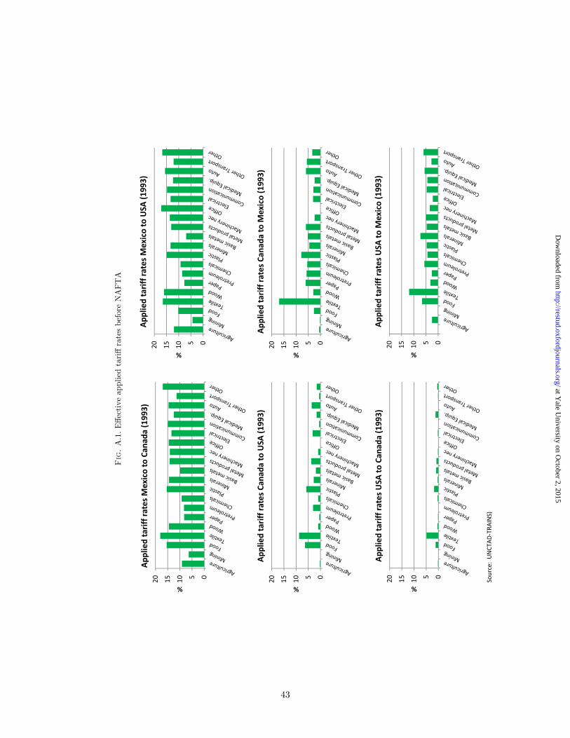
05101520 %

Applied tariff rates M

exico to USA

(1993)

05101520 %

Applied tariff rates Can

ada to USA

(1993)

05101520 %

Applied tariff rates Can

ada to M

exico(1993)

05101520 %

Applied tariff rates USA

to Can

ada(1993)

05101520 %Ap

plied tariff rates USA

to M

exico(1993)

05101520 %Ap

plied tariff rates M

exico to Can

ada (1993)

Source: UNCT

AD‐TRA

INS)

Fig

. A

.1. Effec

tive

appl

ied

tariff r

ates

bef

ore

NA

FT

A

43

at Yale U



ownloaded from


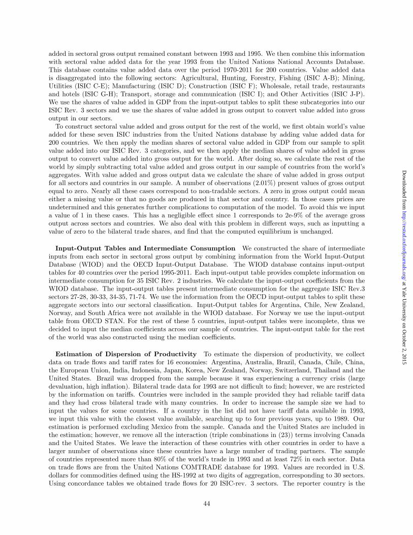
added in sectoral gross output remained constant between 1993 and 1995. We then combine this informationwith sectoral value added data for the year 1993 from the United Nations National Accounts Database.This database contains value added data over the period 1970-2011 for 200 countries. Value added datais disaggregated into the following sectors: Agricultural, Hunting, Forestry, Fishing (ISIC A-B); Mining,Utilities (ISIC C-E); Manufacturing (ISIC D); Construction (ISIC F); Wholesale, retail trade, restaurantsand hotels (ISIC G-H); Transport, storage and communication (ISIC I); and Other Activities (ISIC J-P).We use the shares of value added in GDP from the input-output tables to split these subcategories into ourISIC Rev. 3 sectors and we use the shares of value added in gross output to convert value added into grossoutput in our sectors.To construct sectoral value added and gross output for the rest of the world, we first obtain world’s value

added for these seven ISIC industries from the United Nations database by adding value added data for200 countries. We then apply the median shares of sectoral value added in GDP from our sample to splitvalue added into our ISIC Rev. 3 categories, and we then apply the median shares of value added in grossoutput to convert value added into gross output for the world. After doing so, we calculate the rest of theworld by simply subtracting total value added and gross output in our sample of countries from the world’saggregates. With value added and gross output data we calculate the share of value added in gross outputfor all sectors and countries in our sample. A number of observations (2.01%) present values of gross outputequal to zero. Nearly all these cases correspond to non-tradable sectors. A zero in gross output could meaneither a missing value or that no goods are produced in that sector and country. In those cases prices areundetermined and this generates further complications to computation of the model. To avoid this we inputa value of 1 in these cases. This has a negligible effect since 1 corresponds to 2e-9% of the average grossoutput across sectors and countries. We also deal with this problem in different ways, such as inputting avalue of zero to the bilateral trade shares, and find that the computed equilibrium is unchanged.

Input-Output Tables and Intermediate Consumption We constructed the share of intermediateinputs from each sector in sectoral gross output by combining information from the World Input-OutputDatabase (WIOD) and the OECD Input-Output Database. The WIOD database contains input-outputtables for 40 countries over the period 1995-2011. Each input-output table provides complete information onintermediate consumption for 35 ISIC Rev. 2 industries. We calculate the input-output coeffi cients from theWIOD database. The input-output tables present intermediate consumption for the aggregate ISIC Rev.3sectors 27-28, 30-33, 34-35, 71-74. We use the information from the OECD input-output tables to split theseaggregate sectors into our sectoral classification. Input-Output tables for Argentina, Chile, New Zealand,Norway, and South Africa were not available in the WIOD database. For Norway we use the input-outputtable from OECD STAN. For the rest of these 5 countries, input-output tables were incomplete, thus wedecided to input the median coeffi cients across our sample of countries. The input-output table for the restof the world was also constructed using the median coeffi cients.

Estimation of Dispersion of Productivity To estimate the dispersion of productivity, we collectdata on trade flows and tariff rates for 16 economies: Argentina, Australia, Brazil, Canada, Chile, China,the European Union, India, Indonesia, Japan, Korea, New Zealand, Norway, Switzerland, Thailand and theUnited States. Brazil was dropped from the sample because it was experiencing a currency crisis (largedevaluation, high inflation). Bilateral trade data for 1993 are not diffi cult to find; however, we are restrictedby the information on tariffs. Countries were included in the sample provided they had reliable tariff dataand they had cross bilateral trade with many countries. In order to increase the sample size we had toinput the values for some countries. If a country in the list did not have tariff data available in 1993,we input this value with the closest value available, searching up to four previous years, up to 1989. Ourestimation is performed excluding Mexico from the sample. Canada and the United States are included inthe estimation; however, we remove all the interaction (triple combinations in (23)) terms involving Canadaand the United States. We leave the interaction of these countries with other countries in order to have alarger number of observations since these countries have a large number of trading partners. The sampleof countries represented more than 80% of the world’s trade in 1993 and at least 72% in each sector. Dataon trade flows are from the United Nations COMTRADE database for 1993. Values are recorded in U.S.dollars for commodities defined using the HS-1992 at two digits of aggregation, corresponding to 30 sectors.Using concordance tables we obtained trade flows for 20 ISIC-rev. 3 sectors. The reporter country is the

44

at Yale U



ownloaded from


importer, and imports are at CIF. values. Data on tariffs are from UNCTAD-TRAINS for 1989-1995. Tariffsrepresent the effective tariff rate applied by each country. Tariffs are available for industries at four digitsISIC-rev.3. and were aggregated up to two digits using a weighted average, where the weights are given bythe import values. Whenever data on bilateral tariffs are not available in 1993, we input this value withthe closest value available, searching up to four previous years. The total number of observations for the 20sectors is 9138, with an average of 457 observations per sector.

45

at Yale U



ownloaded from


APPENDIX: ADDITIONAL RESULTS

Table A.2. Dispersion-of-productivity estimates (with importer and exporter fixed effects)Full sample 99% sample 97.5% sample

Sector θj s.e. N θj s.e. N θj s.e. NAgriculture 8.59 (2.00) 496 9.54 (2.11) 430 16.97 (2.48) 364Mining 14.83 (2.87) 296 11.96 (3.84) 178 14.84 (4.38) 152ManufacturingFood 2.84 (0.57) 495 3.02 (0.57) 429 2.89 (0.65) 352Textile 5.99 (1.24) 437 8.55 (1.38) 314 0.61 (1.89) 186Wood 10.19 (2.24) 315 10.72 (2.63) 191 9.30 (2.82) 148Paper 8.32 (1.66) 507 15.20 (2.69) 352 0.51 (2.86) 220Petroleum 69.31 (19.32) 91 68.47 (19.08) 86 65.92 (19.51) 80Chemicals 3.64 (1.75) 430 3.23 (1.76) 341 -0.02 (2.07) 220Plastic 0.88 (1.57) 376 3.10 (2.24) 272 1.95 (2.22) 180Minerals 3.38 (1.54) 342 3.03 (1.73) 263 3.85 (2.07) 186Basic metals 6.58 (2.28) 388 0.88 (2.58) 288 -1.31 (2.77) 235Metal products 5.03 (1.93) 404 7.30 (2.01) 314 0.82 (2.83) 186Machinery n.e.c. 2.87 (1.85) 397 3.88 (3.14) 290 0.70 (4.24) 186Offi ce 13.88 (2.21) 306 9.85 (5.60) 126 21.57 (5.78) 62Electrical 11.02 (1.46) 343 13.95 (1.66) 269 4.66 (2.82) 177Communication 4.86 (1.69) 312 3.27 (2.07) 143 3.33 (2.19) 93Medical 7.63 (1.22) 383 7.49 (1.48) 237 2.45 (1.25) 94Auto 0.49 (0.91) 237 1.59 (1.04) 126 -2.13 (1.34) 59Other Transport 0.90 (1.16) 245 0.91 (1.15) 226 1.05 (1.22) 167Other 4.95 (0.92) 412 3.52 (1.04) 227 2.61 (0.81) 135

46

at Yale U



ownloaded from


Table A.3. Welfare effects from NAFTA’s tariff reductions


Volumeoftrade


Volumeoftrade

Argentina 0.001% 0.000% 0.001% Ireland -0.018% -0.012% -0.006%Australia 0.000% 0.000% -0.000% Italy -0.004% -0.003% -0.001%Austria -0.004% -0.002% -0.002% Japan -0.007% -0.005% -0.002%Brazil -0.002% -0.002% 0.000% Korea -0.029% -0.018% -0.011%Chile 0.010% 0.009% 0.001% Netherlands -0.005% -0.003% -0.002%China -0.028% -0.006% -0.022% New Zealand 0.002% 0.002% -0.000%Denmark -0.002% -0.001% -0.001% Norway 0.003% 0.004% -0.001%Finland -0.001% 0.000% -0.001% Portugal -0.003% -0.002% -0.001%France -0.004% -0.003% -0.001% South Africa 0.003% 0.002% 0.002%Germany -0.005% -0.003% -0.001% Spain -0.008% -0.004% -0.001%Greece 0.000% 0.001% -0.000% Sweden -0.009% -0.006% -0.002%Hungary -0.003% -0.002% -0.002% Turkey -0.001% -0.001% -0.001%India -0.005% -0.002% -0.003% U.K. -0.005% -0.003% -0.002%Indonesia -0.001% 0.000% -0.001% ROW -0.003% -0.001% -0.002%

Table A.4. Welfare effects from NAFTA’s tariff reductions, with trade deficitWelfare


Table A.5. Bilateral welfare effects from NAFTA’s tariff reductions, with trade deficitTerms of trade Volume of Trade

Country NAFTA Rest of the world NAFTA Rest of the worldMexico -0.39% -0.02% 1.69% -0.10%Canada -0.08% -0.01% 0.08% -0.04%U.S. 0.03% 0.02% 0.04% -0.00%

47

at Yale U



ownloaded from


Table A.6. Sectoral contribution to welfare effects from NAFTA’s tariff reductions, with trade deficitMexico Canada United States

SectorTermsoftrade

Volumeoftrade

Termsoftrade

Volumeoftrade

Termsoftrade

Volumeoftrade

Agriculture 0.77% 3.00% 2.06% 0.05% 3.47% 0.79%Mining -0.03% 0.21% 0.58% -0.02% 2.08% 0.07%ManufacturingFood 0.92% 1.17% 2.74% 3.00% 3.30% 1.21%Textile 3.54% 12.30% 1.11% 20.00% 4.84% 23.20%Wood 0.38% 2.26% 1.65% 0.34% 0.99% 0.47%Paper 0.54% 3.78% 4.16% 0.93% 2.32% 0.44%Petroleum 0.17% 15.20% 0.43% 18.90% 0.51% 10.30%Chemicals 1.39% 2.09% 5.90% 0.73% 6.05% 1.35%Plastic 0.82% 4.22% 2.83% 8.77% 1.71% 0.36%Minerals 0.29% 0.75% 0.99% 0.94% 0.81% 0.67%Basic metals 1.51% 2.97% 9.50% 1.61% 3.13% 1.16%Metal products 1.07% 5.59% 2.76% 9.19% 1.76% 1.25%Machinery n.e.c. 4.17% 4.28% 6.14% 0.20% 6.61% 0.78%Offi ce 6.54% 4.53% 2.46% -0.79% 4.31% 1.31%Electrical 36.30% 25.00% 1.75% 7.30% 21.40% 39.50%Communication 20.00% 3.64% 2.82% 0.34% 12.10% 4.85%Medical 4.44% 1.33% 1.25% -0.12% 3.84% 4.65%Auto 14.10% 4.90% 33.10% 29.40% 15.40% 5.16%Other Transport 0.22% 0.80% 17.30% -1.12% 2.15% 0.43%Other 2.87% 1.99% 0.44% 0.39% 3.17% 2.00%

48

at Yale U



ownloaded from


Table A.7. : Sectoral composition of exports, with trade deficitMexico Canada United States



49

at Yale U



ownloaded from


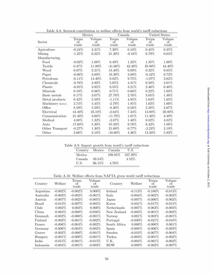
Table A.8. Sectoral contribution to welfare effects from world’s tariff reductionsMexico Canada United States

SectorTermsoftrade

Volumeoftrade

Termsoftrade

Volumeoftrade

Termsoftrade

Volumeoftrade

Agriculture -0.24% 3.31% 7.39% 0.10% 0.45% 0.25%Mining -1.25% 0.32% 21.20% -0.16% 6.79% 0.04%ManufacturingFood -0.02% 1.08% 6.49% 1.32% 1.35% 1.00%Textile 0.47% 11.80% -41.60% 42.30% 35.00% 44.40%Wood 0.07% 2.21% 18.40% 0.89% 0.32% 0.85%Paper -0.06% 3.89% 16.30% 3.00% -0.42% 0.73%Petroleum -0.11% 14.40% 0.82% 9.75% -1.07% 3.62%Chemicals -0.76% 2.80% 5.05% 4.31% 0.50% 2.61%Plastic -0.85% 3.95% 0.55% 3.21% 2.46% 0.40%Minerals 0.10% 0.86% 0.71% 0.66% 0.22% 1.03%Basic metals 0.17% 3.07% 27.70% 2.76% 3.05% 1.46%Metal products 0.42% 5.50% -1.11% 4.85% 1.64% 1.65%Machinery n.e.c. 2.74% 4.45% -2.79% 1.85% 1.02% 1.00%Offi ce 8.59% 5.59% -8.30% 0.56% 5.28% 2.67%Electrical 44.40% 23.10% -2.64% 7.34% 13.80% 20.80%Communication 21.40% 3.60% -11.70% 1.01% 11.30% 3.49%Medical 4.88% 1.32% -2.87% 1.40% 0.82% 4.82%Auto 17.60% 5.30% 55.50% 9.76% 6.42% 1.08%Other Transport -0.27% 1.30% 21.60% 0.77% -2.23% 2.19%Other 2.66% 2.10% -10.60% 4.36% 13.20% 5.93%

Table A.9. Import growth from world’s tariff reductionsCountry Mexico Canada U.S.Mexico 109.85% 107.29%Canada 49.54% 4.52%U.S. 96.15% 4.76%

Table A.10. Welfare effects from NAFTA given world tariff reductions


Volumeoftrade


Volumeoftrade

Argentina -0.002% -0.002% 0.000% Ireland -0.113% -0.100% -0.013%Australia -0.003% -0.002% -0.001% Italy -0.004% -0.002% -0.002%Austria -0.007% -0.002% -0.005% Japan -0.007% -0.006% -0.002%Brazil -0.012% -0.007% -0.005% Korea -0.031% -0.017% -0.015%Chile 0.002% 0.002% 0.000% Netherlands -0.007% -0.003% -0.003%China -0.063% -0.008% -0.056% New Zealand -0.003% -0.001% -0.002%Denmark -0.002% -0.000% -0.001% Norway 0.001% 0.002% -0.001%Finland -0.003% -0.001% -0.002% Portugal -0.030% -0.021% -0.010%France -0.006% -0.004% -0.002% South Africa 0.000% -0.000% 0.001%Germany -0.006% -0.004% -0.002% Spain -0.008% -0.006% -0.003%Greece -0.002% -0.000% -0.001% Sweden -0.010% -0.007% -0.004%Hungary -0.001% -0.000% -0.001% Turkey -0.003% -0.001% -0.002%India -0.015% -0.001% -0.015% U.K. -0.004% -0.001% -0.003%Indonesia -0.004% -0.001% -0.003% ROW -0.009% -0.002% -0.007%

50

at Yale U



ownloaded from


Table A.11. Sectoral contribution to welfare effects from NAFTA given world tariff changesMexico Canada United States

SectorTermsoftrade

Volumeoftrade

Termsoftrade

Volumeoftrade

Termsoftrade

Volumeoftrade

Agriculture 0.03% 3.10% 3.14% 0.02% 3.69% 0.81%Mining -2.73% 0.25% 3.03% -0.21% 0.80% 0.06%ManufacturingFood 0.56% 1.29% 3.41% 3.71% 3.72% 1.31%Textile 3.66% 12.30% 0.52% -4.65% 4.46% 16.50%Wood 0.34% 2.30% 3.41% 0.36% 1.13% 0.57%Paper 0.46% 3.96% 5.48% 0.85% 3.50% 0.53%Petroleum -0.04% 13.40% 0.62% 40.00% 1.98% 12.10%Chemicals 0.77% 2.27% 5.93% 0.37% 6.77% 1.49%Plastic 0.71% 4.50% 2.64% 11.00% 1.44% 0.40%Minerals 0.09% 0.80% 0.97% 0.69% 0.65% 0.74%Basic metals 1.22% 3.24% 10.00% 2.23% 3.09% 1.34%Metal products 0.98% 5.82% 2.42% 10.20% 1.53% 1.38%Machinery n.e.c. 3.80% 4.58% 5.55% 0.13% 5.91% 0.82%Offi ce 7.56% 3.09% 2.27% -1.06% 3.49% 1.34%Electrical 40.50% 26.60% 1.40% 1.45% 22.40% 42.70%Communication 20.20% 3.67% 2.35% 0.20% 11.30% 5.12%Medical 4.55% 1.29% 1.08% -0.81% 3.20% 4.80%Auto 14.40% 4.91% 30.90% 37.80% 17.00% 5.48%Other Transport 0.21% 0.62% 14.30% -1.86% 1.75% 0.47%Other 2.75% 2.06% 0.63% -0.44% 2.19% 2.08%

51

at Yale U



ownloaded from


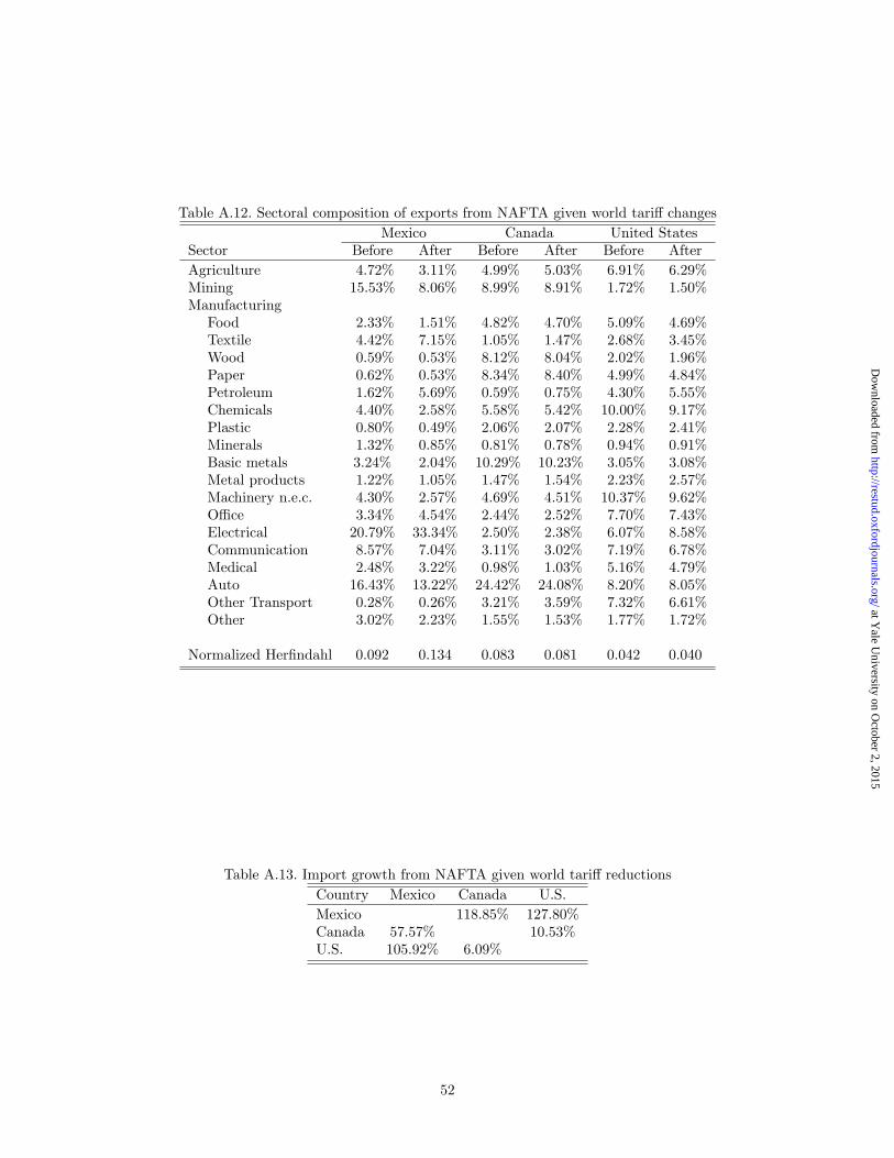
Table A.12. Sectoral composition of exports from NAFTA given world tariff changesMexico Canada United States



Table A.13. Import growth from NAFTA given world tariff reductionsCountry Mexico Canada U.S.Mexico 118.85% 127.80%Canada 57.57% 10.53%U.S. 105.92% 6.09%

52

at Yale U



ownloaded from


estimates of the trade and welfare e⁄ects of...

Documents