Singapore Centre for Applied and Policy Economics

Department of Economics SCAPE Working Paper Series

Paper No. 2013/01 – February 2013 http://www.fas.nus.edu.sg/ecs/pub/wp-scape/1301.pdf

Estimating bubbles and affordable housing price trends: A study based on Singapore

by

Tilak Abeysinghe and Jiaying Gu

   

Estimating bubbles and affordable housing price trends:  A study based on Singapore 

Tilak Abeysinghea,* and Jiaying Gub 

a Department of Economics National University of Singapore AS2, 1 Arts Link, Singapore 117570 

Email: tilakabey@nus.edu.sg, Ph +65 6516 6116  

b Department of Economics University of Illinois at Urbana‐Champaign 

IL61820, USA Email: gu17@illinois.edu  

February 2013 

Abstract 

Policy makers often  impose  some  cooling measures on  the housing market when housing prices  rise fast. Such policies yield limited success if housing prices are driven up by fundamentals. A fundamental price  trend may not necessarily be an affordable one. Unaffordable housing price  trends  increase  the mortgage burden of households. Estimating these different price trends provides valuable  information to policy makers. This paper presents an empirical methodology to separate out a housing price trend into  fundamental  and  affordable  components.  The  gap  between  actual  and  fundamental  trend  is attributed  to  expectations  driven  persistence  of  housing  price  inflation.  This  is  the  component  that cooling measures are usually aimed at. Affordable housing price trend is defined in terms of a measure of lifetime income. Affordability requires the house price to lifetime income ratio to be stationary with a certain mean. Fundamentals need to be adjusted to obtain this outcome. Analyzing Singapore data using this methodology reveals some interesting observations.  

Key Words: Fundamental housing price, affordable housing price, lifetime income, counter‐factual simulations 

JEL Classification: R21, D31. 

‐‐‐‐‐‐‐‐‐ 

* Corresponding author, Tilak Abeysinghe 

 

1. Introduction 

Although  house  prices  are well  known  to  form  bubbles,  separating  the  bubble  and  non‐bubble 

components  is a challenging  task because of  the difficulty of working out a  reference price  level  that 

represents the unobserved non‐bubble component.  There are various definitions of asset price bubbles 

but  from  an  operational  point  of  view we  align with  those who  define  bubbles  in  relation  to  some 

fundamental  variables  (see  Siegel,  2003  for  some  references).  By  this  definition  the  fundamentals 

determine  the  non‐bubble  component  of  the  price  level.  One  question  is  how  to  estimate  this 

fundamental price level. A price level determined by the fundamentals, however, may not necessarily be 

an affordable price  level. For example, population pressures tend to drive city house prices well above 

affordable  levels. Another  important question,  therefore,  is how  to determine  an  affordable housing 

price  level. The objective of this exercise  is to develop an empirical methodology to answer these two 

questions and analyze housing price data from Singapore.   

Singapore is an interesting case study in this regard. The country has a small private housing sector 

and  a  large  public  housing  sector  with  private  ownership.  Singapore  has  one  of  the  highest  home 

ownership rates (about 90%) in the world. Singapore government desires to see house prices appreciate 

over time at an affordable rate. Through home ownership the government  is trying to achieve a social 

objective of “heartland‐feeling” in this global city. Despite regular interventions by the government,1 the 

Singapore housing market has gone through a number of price cycles with prices escalating way beyond 

any  expectation.  Persistent  unaffordable  increase  in  housing  prices  may  bring  about  unexpected 

negative consequences. For example, Abeysinghe and Choy (2007) observed that in Singapore increasing 

housing  wealth  as  a  result  of  increasing  housing  prices  does  not  create  a  positive  impact  on 

consumption  expenditures  because  of  a  lack  of  monetizing  opportunities  of  housing  wealth.  They 

                                                            1 See Gu (2008) and Lum (2011) for a review of Singapore government policies in the housing market. 

2  

observed, however, that increasing housing prices render a substantial negative effect on consumption 

expenditures  leading  to  a  substantial  secular drop  in  average propensity  to  consume  (APC).  This has 

exposed the economy more to volatile external forces.  Yi and Zhang (2010) observed that rising housing 

prices  in Hong Kong as a major cause for the precipitous decline of the state’s total fertility rate (TFR).  

Abeysinghe (2011) noted similar results for Singapore.  The negative impact of rising housing prices may 

not be  limited  to  these  areas.   When house prices  appreciate  it  is not  clear  exactly what drives  the 

appreciation, fundamentals or something else. In this respect the results of this paper provide important 

guidelines to the policy makers. 

There  is  a  sizable  literature  on  modeling  residential  property  prices.  Under  the  so‐called  first 

generation models  pioneered  by Muth  (1960)  followed  by  others  like  Smith  (1969)  stock  and  flow 

demand  for housing was modeled under  the assumption of a highly elastic housing supply. Obviously 

these  models  underwent  the  scrutiny  of  others  for  many  shortcomings.  This  gave  rise  to  further 

improvements under the next generation models that used either the stock‐flow framework or the asset 

pricing  approach.  This  led  to  incorporating more  comprehensive measures  of  user  cost  of  housing, 

supply side features, disequilibrium, demand side expectations, supply side expectations, house vacancy 

rate specifications, and  land supply  issues.2 We  incorporate some key features of this  literature to our 

modeling strategy but depart from the literature in the way we address the two main questions raised 

earlier.  

The methodology  of  estimating  the  fundamental  housing  price  trend  is  discussed  in  Section  2.1. 

Since buying a house is a long term commitment, housing affordability has to be measured in relation a 

measure  of  permanent  income.  The  income  measure  we  propose  is  lifetime  income  and  the 

methodology  of  obtaining  estimates  of  lifetime  income  for  different  income  deciles  is  presented  in                                                             2 To cite a few: Poterba (1984), Case and Shiller (1987), Smith, Rosen and Fallis (1988), Topel and Rosen (1988), Mankiw and Weil (1989), Dipasquale and Wheaton (1994), Mayer and Somerville (2000), Malpezzi and Maclennan (2001), Hwang and Quigley (2006). Gu (2008) provides an extensive literature review. 

3  

Section  2.2. We  propose  to measure  housing  affordability  in  relation  to  the  growth  rate  of  lifetime 

income.  Section  3  provides  a  description  of  computational  methods  of  the  variables  used  in  our 

regressions. Readers may skim through this section to pick up the variable notations and move on to the 

empirical results of sections 4 and 5 directly. Section 6 provides a summary of the methodology and the 

key findings from the analysis of the Singapore housing prices. 

 

2. Methodology 

2.1 Estimating the fundamental housing price level  

There  are  three  price  levels  that  we  need  to  consider,  equilibrium  housing  price,  fundamental 

housing price  and  affordable housing price.  Equilibrium housing price  is usually  expressed  through  a 

present value  relationship  that  is often used  to model house price‐to‐rent  ratio  (Meese and Wallace, 

1994;  Schreyer,  2009;  Igan  and  Loungani,  2012). Holly  et  al.  (2010)  converted  this  relationship  to  a 

house price‐to‐income ratio. This transformation requires the price‐income ratio to be stationary. As we 

shall  see  later,  the  price‐income  ratio  is  unlikely  to  be  stationary  in  situations  where  housing 

affordability  has  been  deteriorating.  To  remove  this  non‐stationarity  we  have  to  introduce  other 

fundamental variables into the model.  

In a simple one period setting  the equilibrium housing price  is obtained by equating the expected 

rate of  return  from home ownership  to  the  rate of homeowner  cost of  capital  (Meese  and Wallace, 

1994). In order to model log‐transformed variables it would be easier to work with the log‐linear present 

value formulation that Campbell and Shiller (1988) introduced for financial assets.3 To stick to the same 

symbols  let   be  the  log of house price  and lntp = tP tDlntd =  be  the  implicit  rental  (dividend)  for 

                                                            3 See Cochrane (2005) for a textbook treatment and Campbell (2008) and Engsted et al. (2012) for further assessments of the transformation. 

4  

owner occupied housing. When the price‐rent ratio  is stationary the Campbell‐Shiller approximation to 

log  return  is     1 1 1ln[( ) / ]t t tr P D+ + += + tP ≈   1 1(1 )t tk p d tpρ ρ+ ++ + − −   = 

1( ) (t t t tk p d d p 1 1)tdρ+ +− − + Δ + +− 1/ (1, where  /P )Dρ = +   and   is a constant. Here   is the 

steady  state  level  of  the  price‐rent  ratio.  In  equilibrium  the  rate  of  return  is  equal  to  the  rate  of 

homeowner  cost  of  capital.  Therefore, writing  the  above  equation  for 

k /P D

t tp d− ,  solving  forward  and 

taking expectation leads to the present value formulation: 

            (1) 1

1( )j

t t j t jj

E d rρ ρ∞

−+ +

=

⎡ ⎤Δ −⎢

⎣ ⎦∑/ (1 )t tp d k− = − +

t

⎥

Ewhere    indicates  expectation  conditional  on  information  at  t.  This  fundamental  bubble‐free 

formulation  shows  that  the price‐rent  ratio, apart  from  the  constant  term,  is  the discounted present 

value of the expected rent growth rate adjusted for the homeowner cost of capital. 

In  general    and    are  I(1)  variables  and  the  formulation  in  (1)  requires    to  be  I(0). 

Although  the  price‐income  ratio  is  our  primary  focus  as  in Holly  et  al.  (2010),  it may  not  be  an  I(0) 

variable as  in the case of Singapore. We can, however, replace   with 

tp td t tp d−

txβ ′td tx, where    is a vector of 

fundamental  variables,  including  income,  such  that  tp β ′− tx   is  I(0).4  The  expectation  term  in  (1) 

involves I(0) variables which are not observed. Both rational expectations (Hansen and Sarget, 1980) and 

extrapolative expectations  (Lansing, 2006, 2010; Granziera and Kozicki, 2012) show  that  the expected 

term  in (1) can be replaced with relevant observed  I(0) variables. Therefore, we can formulate a more 

general econometric model within the cointegrating and error correction model (ECM) framework. 

                                                            4 Usually these variables are expressed in real terms. The inflation effect, however, cancels out in the formulation in (1). Apart from this, we prefer modeling in nominal terms because the consumer price index (CPI) tends to increase when house prices increase and the real house price (P/CPI) tends to be over deflated especially during housing price bubbles. 

5  

  Our  first  question  is  how  to  estimate  the  long  run  price  level  based  on  its  fundamental 

determinants.    Let  *0t tp xβ β′= +   be  the  long  run  (log)  price  determined  by  a  k×1  vector  tx of  the 

fundamental variables.  As mentioned above, we require 

0tp xt tuβ β ′= + +                    (2) 

to be  a  cointegrating  relationship  such  that  . Although we  can obtain  the estimates of  the 

parameters in (2) either using OLS or some other method, the predicted price 

~ (0)tu I

0ˆ ˆˆ tp txβ β ′= +  is not the 

*tp   that we  are  looking  for.  Since  these  parameter  estimates  are  obtained  such  that  u 0t =∑   the 

predicted price line will pass through the center of   line. When price bubbles are present the  line 

will  invariably  lie  above  the 

tp ˆ tp

*tp   line.5 This does not help us  in  gauging  the price  gap  *( )ttp p−   that 

would be of policy interest.  

  One way to estimate  *tp  is to specify an ECM of the form  

0 11 1 0

[p pm

t i t i t ji jt i t t ti j i

p p z x p x 1]φ φ γ δ α β− − −= = =

′Δ = + Δ + + Δ + − +∑ ∑∑ ε−′       (3) 

where    is  a  vector  of  short‐run  determinants  of  house  price  inflation  such  as  the  indicators  of 

speculative activities  in the housing market. The  lagged dependent variables, 

tz

,t ip −Δ  capture the short 

run persistence of housing price  inflation. Such persistence may result  from price expectations. When 

house prices are rising fast the buyers may rush to buy a house because of the fear of further increase in 

price, which will drive prices further up. When house prices are falling buyers may delay the purchase of 

a  house  with  the  hope  that  the  prices may  fall  further,  which  will  accentuate  the  price  fall.  Such 

                                                            5 The opposite will happen if negative bubbles (troughs) are dominant. 

6  

persistence may cause short run deviations of housing price  from  the  fundamental price or may even 

lead to the formation of price bubbles through the interaction of other factors (Glaeser et al., 2008).    

  If (3) is well specified, a dynamic simulation using the full model in (3) will track the actual   very 

closely.  If we  set 

tp

0iφ γ= =  what  is  left  in  (3) are  the  fundamental determinants of  the house price 

inflation. We can therefore obtain  *tp as 

* *0 1

1 0(1 )

pm

t t ji jt i tj i

1p p xφ α δ αβ− −= =

x −′= + + + Δ −∑∑ .          (4) 

Given  1 0α− ≤ <

*t

, a dynamic simulation using  (4) will yield a  long  run price  that will converge  to  the 

same price  p  regardless of the starting point  *0p . The trend of the price line is determined by that of

txβ ′ .  

  While  *tp   is determined by fundamental demand‐supply forces there could be another price  level 

**tp   that  could  be  deemed  desirable  in  terms  of  sustaining  housing  affordability.    When  demand 

pressure  outstrips  the  supply,  *tp will  rise  faster  than **

tp .  Obviously  a  persistent  positive  gap  of

*( )t tp p−  or  **( t t )p p− indicates a buildup of household mortgage debt.   We  can define  **tp  as  the 

price  level  that  renders    stationary. Here    is  a measure  of  household  income.  In  other 

words,   should share the same trend as that of  . In this context what measure of   that we 

should consider becomes important.  

ln( /t )tP Y tY

lnln tP tY tY

    

 

 

7  

2.2 Estimating lifetime income (W) for assessing housing affordability 

A convenient choice for income is per capita disposable income ( ). One problem of using this in 

the assessment of housing affordability is that   is a measure of average income. As income inequality 

increases the average income biases towards higher income groups. A more robust choice would be the 

median income, or some quantile measures of income.

tYd

t

tYd

6  Another problem of using   is that   

does not correspond to the often used mortgage payment to income ratio for affordability assessment. 

Both  these measures  focus on short run affordability. For  this reason Abeysinghe and Gu  (2011) have 

proposed a lifetime income measure ( ) and used the ratio  to assess housing affordability. This 

ratio under some conditions is the same as the standard measure of mortgage payment to income ratio; 

but it has some advantages over the latter. Typically a price‐income ratio less than 30% is taken to mean 

affordable housing prices.  

tYd /t tP Yd

tW /tP W

  Lifetime  income  is the discounted present value of the future  income stream of a household or an 

individual. For this we require the age‐income profile of a household or an individual. When income data 

by age and year are available  it  is possible  to  trace  the  income of  the same birth cohort as  they age. 

However, given the  limited data available, complete age‐income profiles can be constructed only for a 

few cohorts. Incomplete age‐income profiles have to be filled using predicted values from a regression. 

The regression that Abeysinghe and Gu (2011) adapted from Moffitt (1984)) to estimate the age‐income 

profile of a representative household in a birth cohort can be written as: 

120 1 2 2

A Tit i i k k itk

y Age Age Cα α α γ+ −

== + + + +∑ ε

                                                           

            (5) 

 6 If income (y) is lognormally distributed or log of income is normally distributed with mean μ  and variance  2σ , 

then 20.5( )E y eμ σ+=  and Median(y)=Md(y)= eμ . This gives, 

20.5( ) / ( )E y Md y e σ= and as the variance of log‐

income distribution increases the mean departs from the median at the rate given above. 

8  

where i=1,2,…,A is the ith age representing year in index form, t=1,2,…,T is the tth year index, k=A‐i+t is 

the kth cohort  index, ’s are cohort dummies and    is  the  log of average household  income. Note 

that the income data for (5) are arranged in a panel format, for each age i, t=1,2,…,T. The quadratic age 

term  captures  the  usually  observed  hump‐shaped  age‐income  profile  of  a  household.  The  cohort 

dummies allow for shifts in the age‐income profile from one birth cohort to another.  

kC ity

If  income by household  is available annually  then  the quantile  regression  technique proposed by 

Koenker and Bassett (1978) can be used to obtain quantile coefficient estimates of (5) and then derive 

the quantile age‐income profiles. The income data available to us are in deciles (see Section 3) and we 

cannot use  the quantile  regression  techniques directly. However, Chamberlain  (1994) has  shown  that 

when the right hand variables of the regression are discrete (as in the case of our regression 5) the least‐

square method  on  group‐specific  quantile  summary  statistics  provides  consistent  estimators  for  the 

regression quantile coefficients and they are asymptotically normally distributed under mild regularity 

conditions  (see  Bassett  et  al.,  2003  and  Chetverikov  et  al.,  2013  for  further  developments  and 

applications). We can, therefore, estimate (5) or its variants discussed below by OLS for different income 

deciles to obtain the quantile age‐income profiles.  

Usually income data are available by age groups, say L years (usually L=5). To correspond to this we 

have to convert years also  into L year groups. If A and T are taken to be multiples of L, then there  is a 

total of  (A/L)(T/L) observations to estimate  (5) with  (A+T)/L‐1 cohort dummies. This grouping provides 

age‐income  profiles  of  different  birth  cohorts  also  at  L‐year  intervals.  Abeysinghe  and  Gu  (2011) 

followed this estimation method and used the spline  interpolation method  in SAS to obtain an annual 

series of lifetime income values.  

An alternative method is not to group years into five‐year intervals, but to introduce enough cohort 

dummies  to  estimate  the  age‐income  profile  at  yearly  intervals. Under  this  setting  there  are  (A/L)T 

9  

observations to estimate (5) with A+T‐L cohort dummies. One disadvantage of the alternative method is 

that  the  number  of  observations  available  for  estimating  the  cohort  coefficients  of  the  older  and 

younger  cohorts  drops  substantially  leading  to more  volatile  cohort  coefficient  estimates.  Since we 

expect  the  lifetime  income  to move  smoothly among  the  consecutive  cohorts we  suggest applying a 

smoothing filter to the annual cohort coefficients.  In this exercise we use a spline smoothing method. 

Fig.  1  shows  the  annual  cohort  coefficient  estimates  from  our  alternative  methodology  and  their 

smoothed values for the median income group. 

6.0

6.2

6.4

6.6

6.8

7.0

7.2

7.4

7.6

7.8

8.0

1945

1947

1949

1951

1953

1955

1957

1959

1961

1963

1965

1967

1969

1971

1973

1975

1977

1979

1981

Birth cohort

 

Fig. 1. Cohort coefficient estimates solid line and their smooth values dashed line for the median income group 

 

 

 

10  

3. Data and computation methods of variables7 

Residential property price (P) 

Singapore’s  residential  property market  has  three major  segments,  private  housing,  new  public 

housing and resale public housing. Private housing caters mainly to high income groups. Public housing 

in  Singapore  is  provided  by  the  Housing  and  Development  Board  (HDB)  and  is  also  known  as  HDB 

housing. New HDB houses are sold to Singapore citizens at a highly subsidized rate. After five years of 

owner occupation  these properties  can be  sold  in  the open market. This  is known as  the HDB  resale 

market. Price data of new HDB properties are not available. Therefore, we study only  the private and 

HDB  resale housing prices. Even  for  these markets  sufficiently  long  time  series are available only  for 

median housing prices. The Urban Redevelopment Authority has published a quarterly private housing 

price  index since 1975 and  the HDB has published a quarterly HDB  resale price  index since 1990. We 

converted these indices to price levels using median price levels of 2005. Fig. 2 presents the private and 

HDB median housing prices. The  large price gap between the two markets and upward trend of prices 

with common cycles are some observations to be noted down.  

                                                            7  Unless otherwise specified the main source of data used in the study is the STS database of the Department of Statistics, Government of Singapore. 

11  

0

200,000

400,000

600,000

800,000

1,000,000

1,200,000

1,400,000

1975

1976

1978

1979

1981

1982

1984

1985

1987

1988

1990

1991

1993

1994

1996

1997

1999

2000

2002

2003

2005

2006

2008

2009

2011

P Private P HDB 

Fig. 2. Private and HDB median housing prices (Singapore $) 

Housing stock (HS) 

Because  of  data  limitations  on  the  number  of  housing  units  available, we  constructed  quarterly 

housing  stock  series  from constant dollar  investment  in private and public housing markets using  the 

perpetual inventory method. This investment‐based housing stock accounts for quality variation in units 

and also  contains  supply‐side expectations. We  lagged  the HDB  series by  five years because  the new 

HDB units can be sold only after five years of owner occupation.  

Population (POP) 

Population  data  are  available  on  an  annual  basis.    Singapore’s  resident  population  consists  of 

Singapore  citizens  and  permanent  residents.  This  component  changes  slowly  and  smoothly.  We 

therefore, used the spline interpolation method in SAS to obtain the quarterly resident population. The 

most  volatile  component  of  the  population  is  non‐permanent  residents.  A  large  proportion  of  this 

population  is foreign workers. We used the  labor force data that are available quarterly to construct a 

12  

quarterly series of working age foreign worker population. The total population is the sum of these two 

components.  In  the  private  housing  price  equation we  used  the  total  population.  In  the  HDB  price 

equation  we  used  the  resident  population  because  HDB  houses  can  be  bought  only  by  Singapore 

residents. 

Lifetime income (W) 

We  obtained  average  household  nominal  income  by  age  and  year  by  income  deciles  from  the 

Department of Statistics, Government of Singapore. Age  is for the household head and  is grouped  into 

five‐year intervals. Annual data are available from 1990. Data from 2000 onwards are available with and 

without employer’s Central Provident Fund (CPF) contributions. The ratio of income with CPF to income 

without CPF  is  about  1.1. We multiplied  the data  prior  to  2000 by  1.1  to  adjust  them  to match  the 

income data with  employer’s CPF  contributions. We  then used  the  alternative methods described  in 

Section 2.2 to construct age‐income profiles by birth cohort for each  income decile. We then obtained 

the discounted present value of household  income over age 30‐64 using  the discount  rate of 5% and 

constructed the  lifetime  income series by birth cohort; birth year plus 30 becomes the reference year. 

As in Abeysinghe and Gu (2011) we use age 30 as the age at which a young couple looks for a residential 

property unit. We denote the lifetime income series thus constructed by W1, W2 …,W9  to refer to the 

defiles 1 to 9. To convert these annual series to quarterly we used the spline  interpolation available  in 

the SAS  software package. Fig. 3 presents  these  lifetime  income  series and  it highlights  the widening 

income gap between the lower and higher income groups that is of interest for a separate study.8  

                                                            8 Note that the series presented in Figure 4 of Abeysinghe and Gu (2011) are in real terms whereas those in Fig. 3 in this paper are in nominal terms. Moreover, the income series of this study includes employer’s CPF contributions that were not available to Abeysinghe and Gu (2011). 

13  

0.0

1.0

2.0

3.0

4.0

5.0

6.0

7.0

1975

1977

1979

1981

1983

1985

1987

1989

1991

1993

1995

1997

1999

2001

2003

2005

2007

2009

2011

W9

W8

W7

W6

W5

W4

W3

W2

W1

 

Fig. 3. Estimated nominal lifetime income (Singapore $mn) of 30‐year old cohorts by income deciles  

Savings 

By age 30 households have some savings that need to be added to the discounted present value of the 

future income stream to obtain the complete lifetime income of a household. Constructing meaningful 

savings  series  by  income  deciles  from  quinquennial  household  expenditure  surveys  is  not  easy. We, 

therefore, use quarterly per capita CPF balances  (overall)  in nominal  terms  to  represent accumulated 

savings. 

Disposable income (Yd) and Deposits (Depst) 

Lifetime income is a slowly changing quantity (Fig. 3). Therefore, to capture short run effects of income 

changes we use per  capita nominal disposable  income  and  residents’ deposits. Disposable  income  is 

calculated  as  in  Abeysinghe  and  Choy  (2007):  GDP  ‐  taxes  ‐  government  fees  &  charges  ‐  net  CPF 

contributions. About 60% of the financial wealth of Singaporean households is made up of CPF balances 

14  

and residents’ deposits. Our empirical analysis shows that between the two the CPF balances is the key 

long run determinant of housing prices but deposits may have some short run effects.  

User cost of housing (UC) 

In empirical exercises the user cost of owner occupied housing (the rate of homeowner cost of capital) is 

often defined as   

[(1 )( ) ]m pUC iτ τ δ π= − + + −                (6) 

where  mτ   is  the marginal  income  tax  rate,  pτ   is  the  property  tax  rate,    is  the  nominal mortgage 

interest rate, 

i

δ   is  the depreciation rate which may be broadly defined  to  include other maintenance 

costs, and π  is expected capital gains (DePasquale and Wheaton, 1994; Igan and Loungani, 2012). The 

marginal income tax rate is included in the equation because property taxes and mortgage payments are 

tax deductible. 

Constructing the user cost of housing is problematic because of the difficulty of measuring expected 

housing price appreciation π .   Since house prices are subject to bubbles, the use of some averages or 

projections  based  on  observed  housing  price  to  represent  expectations  in  the  UC  formula  tend  to 

produce highly volatile UC series with implausible negative values (Schreyer, 2009).  Researchers on this 

problem have found that the trend movements of the consumer price  index (CPI) as providing a much 

better measure of  long term house price expectations  (Poterba, 1992; Schreyer 2009).  In our exercise 

we  also  use  the  trend  movements  of  the  CPI  inflation  rate  to  measure  the  baseline  house  price 

expectations.    After  some  experimentation,  the  baseline  CPI  inflation  rate  was  obtained  by  simple 

exponential smoothing with α =0.2.   

15  

The marginal  income  tax  rate  in  the  UC  formula  was  calculated  as  the  income‐share  weighted 

average  of  the marginal  tax  rates.  Let  iτ   be  the marginal  income  rate  for  the  ith  income  bracket 

i=1,2,…,k,   be the assessed  income of the  ith  income group, and   be the  income share of the  ith 

group. Then the average of the marginal income tax rates, 

iY iw

mτ , can be written as: 

1

Total tax assessedTotal assessed income

ki i

m i ii i

Yw

Yτ

τ τ=

= = =∑∑ ∑           

where  . Total tax assessed and total assessed income are available in the Yearbook of 

Statistics.  

/i iw Y Y= ∑ i

As  for  the  mortgage  interest  rate  i  we  use  the  average  housing  loan  rate  compiled  by  the 

Department  of  Statistics.  This  is  available  since  1983.  For  the  period  before  1983 we  use  the  prime 

lending  rate.  For  HDB  housing  we  take  the  weighted  average  of  the  housing  loan  rate  and  HDB 

concessionary home  loan  rate with a weight of 0.75  for  the  former. We set  the annual value of  δ to 

0.03. The UC series can be computed from 1976Q1 and shows a downward trend; it dropped from more 

than 14% in 1986 to below 1% by the end of 2012. 

Sub‐sale Rate and Foreign Ownership Rate 

An important indicator of speculative activities in the private housing market in Singapore is the sub‐

sale  rate.  This measures  how  frequently  a  new  residential  unit  under  construction  is  sold  before  its 

completion. This data  series  is available only  from 1995Q1. Another  variable  that  is alleged  to  cause 

large price upswings is the inflow of foreign capital to the private housing market (Lum, 2011; Liao et al. 

2012).  Time  series  data  on  capital  inflow  is  not  available.  As  a  proxy  we  use  the  proportion  of 

uncompleted  private  residential  units  purchased  by  foreigners.  These  data  are  available  only  from 

16  

1996Q2.  

 

4. Fundamental housing price trends and bubbles 

To estimate  long run housing price trends determined by the fundamentals we first formulate the 

cointegrating regression (2) as: 

  0 1 2 3 4ln( / ) ln( / ) ln . 08t t t t t tP W HS POP CPF UC UC Dum utβ β β β β= + + + + +   (7) 

The  variables  in  (7)  were  defined  in  the  previous  section  (see  also  notes  to  Table  1).9  Following 

DePasquale  and Wheaton  (1994)  HS/POP  represents  a  given  stock  of  housing  supply  per  capita.  As 

mentioned  in  the previous  section our  investment‐based housing  stock measure  contains  supply  side 

expectations. The other variables represent demand side fundamentals. Unit root tests indicate that the 

variables in (7) can be assumed to be unit root processes. Dum08 in (7) is a step dummy that takes value 

1  from 2008Q1. The  recursive OLS estimates of  3β  become  less stable after 2007 because of a sharp 

drop  in  the UC  variable. With  the  interaction  variable, UC.Dum08,  the  recursive  estimates  of  all  the 

coefficients of (7) become highly stable.10  

Since we have only the median house prices we wanted to assess which lifetime income variables to 

be  used  in  the  regression. We  first  carried  out  a  residual  based ADF  test  for  cointegration  over  the 

sample period 1976‐2007 without  the dummy.  Since private housing  in  Singapore  is  for high  income 

groups we used  the  income  variables  from W5  to W9  in  (7)  for  this  test. We  find  that  cointegration 

cannot be rejected at the 10% level only for the high income groups W8 and W9. As for HDB housing we 

carried  out  this  test  for  income  groups  W1‐W6.  The  residual  based  ADF  test  does  not  support 

                                                            9 Unrestricted estimates show that the coefficient of lnWt can be restricted to unity. 10 Trying to obtain the cointegrating vector in (7) through dynamic models (Bardsen, 1989; Stock 1993; Johansen, 1995) proved unsatisfactory because of the distortionary effects of price bubbles on the estimates. 

17  

cointegration  for  HDB  housing  prices.  This  could  be  due  to  the  shorter  sample  period  1990‐2007. 

Nevertheless we estimated the full regressions and carried out simulations using W8 for private housing 

and W5 for HDB housing. 

The  estimation  results  are  reported  in  Table  1.  The  coefficient  estimates  in  Panel  1  have  the 

expected  signs  and  their  recursive  estimates  are  highly  stable.  Although  the  t‐statistics  of  these 

cointegrating  regressions  may  not  follow  the  normal  distribution  they,  except  for  that  of  UC,  are 

substantially larger than the standard critical values. Recursive estimates of the ECMs in columns (1) and 

(3)  in Panel 2 are also stable and meaningful although some residual diagnostics fail. We retained only 

the statistically significant estimates in these regressions. Although the ADF test rejects cointegration for 

HDB  housing  price,  the  adjustment  coefficient  of  the  EC  term  indicates  that  it  is  a  cointegrating 

relationship though the t‐statistic is not as large as that for the private housing price.11 Column (2) in the 

table was considered to examine the effect of two additional variables (see below). Despite the reduced 

sample size the estimates in column (2) are not very different from those in column (1).    

   

                                                            11 Residual based ADF test for cointegration is well known to have low power. 

18  

Table 1. Regression estimates for private and HDB housing prices 

Private  HDB 

Panel 1: Cointegrating regression 

(1)  (2)  (3) 

Dept variable  ln( / 8 )t tP W   ln( / 5 )t tP W  

Coeff  t‐stat  Coeff  t‐stat 

Constant  ‐0.26  ‐0.67 

Same as Col (1) 

 

 

18.63  11.2 

ln( / )t tHS POP   ‐1.58  ‐14.6  ‐3.55  ‐13.7 

ln tCPF   1.45  17.5  1.37  13.2 

tUC   ‐0.02  ‐1.88  ‐0.02  ‐1.23 

. 0 tUC Dum 8   ‐0.10  ‐6.41  ‐0.09  ‐4.28 

R2  0.82  0.71 

Panel 2: Error correction model 

Dept variable  ln tPΔ   ln tPΔ   ln tPΔ  

Coeff  t‐stat  Coeff  t‐stat  Coeff  t‐stat 

Constant  ‐0.02  ‐2.93  ‐0.02  ‐2.49  0.02  2.33 

1ln tP−Δ   0.64  11.1  0.57  6.89  0.58  7.11 

1tEC −   ‐0.07  ‐4.24  ‐0.06  ‐2.98  ‐0.07  ‐2.66 

ln tHSΔ   ‐  ‐  ‐  ‐  ‐2.20  ‐2.8 

ln tPOPΔ   1.62  2.43  1.13  1.42  ‐  ‐ 

1ln tDepst −Δ   0.43  3.51  0.44  3.88  ‐  ‐ 

ln tYdΔ   0.19  1.99  0.22  2.11  ‐  ‐ 

1ln tYd −Δ   0.22  2.26  0.22  2.00  0.26  2.5 

tSubsaleRateΔ   ‐  ‐  0.002  1.65  ‐  ‐ 

1tForeignOwnershipRate −Δ   ‐  ‐  0.002  1.63  ‐  ‐ 

R2  0.63  0.72  0.52 

Residual diagnostics  test  p‐value  Test  p‐value  test  p‐value 

AR  1.64  0.1537  1.59  0.1927  1.50  0.2003 

ARCH  2.72  0.0325  0.89  0.4756  0.24  0.9174 

Normality   21.50  0.0000  40.37  0.0000  44.06  0.0000 

Hetero   1.53  0.1212  0.96  0.5195  1.02  0.4351 

Hetero‐X   1.87  0.0130  ‐  ‐  0.99  0.4914 

RESET   0.68  0.4124  0.54  0.4673  0.08  0.7767 

Sample period  1976Q1 ‐ 2011Q4  1996Q2 ‐ 2011Q4  1990Q1 ‐ 2011Q4 Note:  P=median  housing  price, W5=household  lifetime  income  of  5th  income  decile, W8=household  lifetime  income  of  8th income decile, CPF=per capita Central Provident Fund balances, HS=housing stock, POP=population, UC=user cost of housing, Depst=per  capita  residents’  deposits,  Yd=per  capita  disposable  income,  EC=error  correction  term  OLS  residuals  from  the cointegrating regression. Residual diagnostics are those readily available in PcGive.  

19  

 

It  is worth  highlighting  some observations  that  emerge  from  Table  1.  First,  for HDB housing  the 

coefficient of per capita housing  stock  is much  larger  in absolute value  than  that  for private housing. 

Although this was not expected apriori, this seems to capture the fact that HDB caters to more than 80% 

of the Singaporean households. Therefore, one percent  increase  in per capita housing stock  is  likely to 

have a much bigger effect on HDB housing prices compared to private housing. Second, short run effects 

of housing stock growth and population growth seem to manifest differently in private and HDB markets 

(Panel 2).  It appears that short run fluctuations  in population affect private housing price  inflation and 

not HDB. This  is understandable because HDB units cannot be bought by  foreigners and they are also 

subject to renting restrictions. On the other hand, an increase in the HDB housing stock lowers the HDB 

housing price  inflation both  in  the  short  run and  long  run. Third,  the effects of  the  sub‐sale  rate and 

foreign ownership rate are not statistically significant. This is partly due to the reduced sample size. The 

sub‐sale  rate  picks  up  the  speculative  activities  in  the  housing  market.  It  dropped  sharply  after 

government interventions in the housing market in 1996. Since then speculation in the housing market 

has  remained  subdued and  the  insignificant effect  for  the  sub‐sale  rate  seems  to  reflect  this. Foreign 

ownership  rate, on  the other hand, does not  seem  to be picking up  the  full  impact of  foreign capital 

inflow to the private housing market. To stimulate the housing market out of its slumber during the mid 

2000s the government relaxed the rules of foreign ownership of residential properties in Singapore. This 

led to a substantial pick up in housing prices subsequently and the government had to tighten the rules 

again (Lum, 2011; Liao et al. 2012). Our proxy variable does not pick up this effect well. 

Fig. 4  shows  the actual median private housing price and  the  fundamental price  trend  simulated 

from regression (1) in Table 1 based on the formulation in (4) using starting values from 1977Q1 and Q2. 

Fig. 4 also shows a simulated (dotted) line with starting values from 1995Q1 and Q2 to highlight that it 

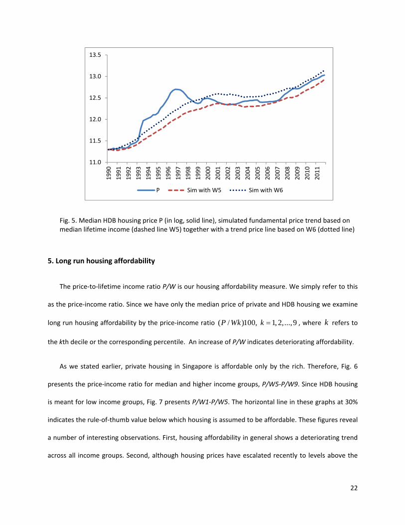
converges to the same trend line regardless of the starting values. Fig. 5 shows the simulated trend line 

20  

for HDB median housing price. Housing price bubbles are clearly visible from these figures, one  in the 

early 1980s and the other in the mid 1990s. Government interventions pricked the bubble of the 1990s 

that resulted in a decade long downward price adjustment before prices started to climb up again above 

the  trend  line since 2007. Between 2007 and 2011 both private and HDB housing prices  increased by 

about 12%  per year whereas fundamental trend price increase should have been about 7% for private 

housing and 10% for HDB housing. It seems that the HDB housing price inflation is mostly fundamental 

driven. Fig. 5 also shows price trend  line generated by plugging  in W6 to the regression (3)  in Table 1. 

Although we need HDB prices for the 6th decile for a proper study, Fig. 5 shows that recently HDB prices 

have moved closer to the price generated for the 6th income decile than to the median trend. This brings 

us to the next question whether the fundamental trend price increases are affordable. 

11.0

11.5

12.0

12.5

13.0

13.5

14.0

14.5

P Sim with W8 

Fig. 4. Median private housing price P (in log, solid line) and simulated fundamental price trend (dashed line W8). Dotted line uses starting value from 1995Q1 and Q2.  

 

21  

11.0

11.5

12.0

12.5

13.0

13.5

1990

1991

1992

1993

1994

1995

1996

1997

1998

1999

2000

2001

2002

2003

2004

2005

2006

2007

2008

2009

2010

2011

P Sim with W5 Sim with W6 

Fig. 5. Median HDB housing price P (in log, solid line), simulated fundamental price trend based on median lifetime income (dashed line W5) together with a trend price line based on W6 (dotted line) 

 

5. Long run housing affordability 

The price‐to‐lifetime income ratio P/W is our housing affordability measure. We simply refer to this 

as the price‐income ratio. Since we have only the median price of private and HDB housing we examine 

long run housing affordability by the price‐income ratio  ( / )100, 1, 2,...,9P Wk k = , where   refers to 

the kth decile or the corresponding percentile.  An increase of P/W indicates deteriorating affordability.  

k

As we  stated earlier, private housing  in Singapore  is affordable only by  the  rich. Therefore, Fig. 6 

presents the price‐income ratio for median and higher income groups, P/W5‐P/W9. Since HDB housing 

is meant for low income groups, Fig. 7 presents P/W1‐P/W5. The horizontal line in these graphs at 30% 

indicates the rule‐of‐thumb value below which housing is assumed to be affordable. These figures reveal 

a number of interesting observations. First, housing affordability in general shows a deteriorating trend 

across all  income groups. Second, although housing prices have escalated recently to  levels above the 

22  

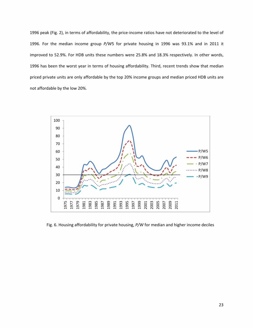
1996 peak (Fig. 2), in terms of affordability, the price‐income ratios have not deteriorated to the level of 

1996.  For  the median  income  group  P/W5  for  private  housing  in  1996  was  93.1%  and  in  2011  it 

improved to 52.9%. For HDB units these numbers were 25.8% and 18.3% respectively.  In other words, 

1996 has been the worst year  in terms of housing affordability. Third, recent trends show that median 

priced private units are only affordable by the top 20% income groups and median priced HDB units are 

not affordable by the low 20%.  

 

0

10

20

30

40

50

60

70

80

90

100

1975

1977

1979

1981

1983

1985

1987

1989

1991

1993

1995

1997

1999

2001

2003

2005

2007

2009

2011

P/W5

P/W6

P/W7

P/W8

P/W9

 

Fig. 6. Housing affordability for private housing, P/W for median and higher income deciles 

23  

0

10

20

30

40

50

60

70

80

90

100

1990

1991

1992

1993

1994

1995

1996

1997

1998

1999

2000

2001

2002

2003

2004

2005

2006

2007

2008

2009

2010

2011

P/W1

P/W2

P/W3

P/W4

P/W5

 

Fig. 7. Housing affordability for HDB housing, P/W for median and lower income deciles 

 

Since 2007 the price‐income ratios have trended upward. We noted in the previous section that the 

median  housing  prices  have  increased  by  about  12%  per  year  between  2007  and  2011  and  the 

fundamental trend price increase should have been about 7‐10%. The average annual growth of median 

lifetime income has been about 4% and that of the 8th income decile has been about 4.3%. These are the 

rates  at  which  relevant  housing  prices  should  have  grown  in  order  to  sustain  long  run  housing 

affordability.   

5.1 Counter‐factual simulations 

From a policy point of view our framework suggests attending to two components of housing price 

inflation in order to keep it in line with the growth of the lifetime income. First is to eliminate short run 

housing price  inflation persistence and the second  is to adjust the fundamental variables. To eliminate 

the short run persistence various governments from time to time have imposed various measures such 

24  

as higher downpayments and additional  stamp duties.  In  the  case of Singapore,  the government has 

introduced  seven  rounds  of  cooling measures  on  the  property market  since  2009.  These measures 

obviously have only limited effects if actions are not taken to address the fundamentals.    

We carried out a number of counter‐factual simulations to see how changes  in some fundamental 

variables  would  have  altered  the  private  and  HDB  median  housing  price  inflation  since  2007. We 

considered  five  scenarios by  fixing  the values  for population, housing  stock and user cost of housing. 

These have to be discussed separately for private and HDB housing.  

For  private  housing we  used  total  population.  The  growth  of  population  is  a  contentious  issue 

among Singaporeans who want to see a drastic reduction in the foreign worker population in Singapore. 

In 2007‐08 Singapore’s resident population grew by about 1.6% while the total population grew by more 

than 4.9% before slowing down to about 2% in 2010‐11. Restrictive immigration and work visa policies 

of the Singapore government are likely to slow down the population growth further. In our simulations 

we  set  the annual  total population growth  rate  to 1.5%. To avoid an abrupt change  in  the  simulated 

values, we  allow  the population  growth  rate  to  steadily decline over  the  quarters of  2007  and  then 

onwards  settle  down  to  1.5%.  The  second  variable  we  consider  is  the  housing  stock.  Singapore 

government  has  been  releasing  more  land  sites  for  private  sector  housing  developments  and  the 

housing investment growth rate has increased to more than 7% in 2011 from a low of 3.8% in 2007Q1. 

Further  increase  in the housing  investment growth rate  is  likely. We, therefore, set this growth rate to 

8% in our simulation. As in the case of population growth we allow the rate to increase steadily in 2007 

before settling to 8%.  The third variable we consider is the user cost of housing. The key factor in the UC 

is  the mortgage  interest  rate which  is market  determined  and  not  subject  to  policy  interventions  in 

Singapore.  We  can,  however,  expect  the  interest  rates  to  pick  up  from  their  rock‐bottom  values 

25  

presently. Our UC value for private housing stood at 6.2% in 2007Q1 and dropped to 1.7% by 2011Q4. In 

our simulations we set the UC value to 6.2% since 2007Q1.  

As  for HDB housing we used  the  resident population Singapore citizens and permanent  residents, 

PRs. Despite many monetary and non‐monetary incentives offered by the government, the fertility rates 

of Singaporeans have been falling. As a result the growth of the Singapore citizen population has slowed 

down to about 0.9% per year since 2005. To compensate for this the government has taken in more PRs. 

From 288,000 in 2000 the PR number increased to 541,000 in 2010 before declining to 532,000 in 2011. 

Because of the unhappiness expressed by Singaporeans on foreigner  inflow, the government plan  is to 

restrict the PR population to about 500,000. Had this been a concern in 2006 we could assume that the 

government would have  frozen  the PR population at  the 2006  level of 418,000. This  is a scenario we 

consider for our counter‐factual simulation over 2007‐2011.  The next policy variable is the HDB housing 

stock. There has been a  substantial  slowing of  the  growth of HDB housing  investment  since  the  late 

1990s; it declined from above 6% growth to about 0.5% growth by 2006. This effect is felt in the HDB re‐

sale market five years later because of the restriction that new units can be sold only after five years of 

owner occupation. The  government  is  currently  in  the process of  increasing  the HDB housing  supply 

substantially. For our simulation we set the housing  investment growth rate to a modest 3%, the rate 

observed  in 2001  that matters  for  the  resale market  in 2006. The  third variable  is UC; we  set  this  to 

2007Q1 value of 5.56%. 

The simulation results are presented in Table 2. The table presents the base line simulation that we 

presented in Fig. 4 and 5 together with other counter‐factual simulations. It presents the average annual 

median housing price inflation rate over 2007‐2011 in each case and the price gap (actual – simulated) 

or the dollar amount by which the median price would have dropped by 2011Q4. Note that we obtained 

26  

the  baseline  simulation  by  removing  inflation  persistence  from  our  ECM model.  The  other  scenarios 

present the additional drops resulting from the adjustments to the fundamental variables. 

The results in Table 2 show that the population growth policy, at least the way we have set it up, is 

the least effective in bringing down the housing price inflation. Obviously limiting the population growth 

rate  requires  a  substantial  reduction  of  the  foreign  worker  population  in  Singapore.  The  results  in 

Abeysinghe  and  Choy  (2007)  based  on  a  comprehensive  macro‐econometric  model  show  that  a 

substantial  reduction  in  the  foreign  worker  population  entails  undesirable  outcomes  like  reduced 

economic growth and high unemployment. Therefore, the foreign worker population as a policy variable 

for the housing market has  limited flexibility. An  increase  in the housing stock works more effectively, 

more  so  in  the  HDB market.  Therefore,  a more  desirable  policy  combination would  be  a moderate 

reduction  in  the population growth and a  reasonably higher growth  in  the housing stock. Obviously a 

pick up  in the user cost of housing to higher  levels while the other two policies are  in place may bring 

down the housing price inflation to affordable rates.  

   

27  

Table 2. Counter‐factual simulations over 2007Q1‐2011Q4 for median housing prices 

Annual house price  inflation rate 2007‐2011

Price gap Sin $ (Actual‐Simulated) 2011Q4Scenario 

Private Housing Actual  11.7  $0 Simulation: Base line‐Fundamental, Fig. 4  7.01  $160,000 (1) Population growth 1.5%  6.38  $193,000 (2) Housing Stock growth 8%  5.81  $234,000 (3) User Cost value 6.2%  5.72  $241,000 (1) and (2)  5.41  $246,000 (1) (2) and (3)  4.37  $303,000 HDB Housing Actual  12.37  $0 Simulation: Base line‐Fundamental, Fig. 5  10.41  $44,000 (1) PR population frozen at 418,000  9.50  $61,000 (2) Housing Stock growth 3%  5.10  $142,000 (3) User Cost value 5.56%  7.12  $108,000 (1) and (2)  4.31  $154,000 (1) (2) and (3)  1.23  $200,000 Note: Hosing stock in this study is the accumulated housing investment. Median housing prices at 2011Q4 for private and HDB units were $1,28 mn and $456,000 respectively.  

 

6. Conclusion 

Unaffordable increases in residential property prices over a long stretch of time may entail unexpected 

negative socio‐economic consequences. Obviously, long term housing affordability has to be assessed in 

relation to a measure of permanent income. The income measure proposed in this study is the lifetime 

income of a household. Extending from Abeysinghe and Gu (2011) we have presented a way to compute 

lifetime  income by  income deciles.  If housing prices  increase at the rate of  lifetime  incomes  long term 

housing affordability is sustained. Otherwise, households will be burdened by excessive mortgage debts. 

Any  increase  in housing prices above this sustainable  level may result primarily from a combination of 

two  other  forces,  other  fundamentals  (e.g.,  supply  shortfall)  and  expectations  driven  persistence  of 

28  

hosing  price  inflation. We  have  presented  a way  to  estimate  the  fundamental  driven  price  level.  If 

housing prices increase faster than the fundamental trend, housing market cooling measures are called 

for.  The  gap  between  fundamental  and  affordable  trends  needs  to  be  addressed  by  adjusting  the 

fundamentals.  

Applying  these  methods  to  analyze  Singapore  residential  property  market  reveals  interesting 

observations. Some key  results are  summarized here. 1. Housing affordability measured by  the price‐

income ratio shows a deteriorating trend across all income groups although price corrections from time 

to time have brought the ratio under the 30% cut‐off value. Recent increases in housing prices are not as 

bad as the 1995‐96 period when viewed  from an affordability point of view. 2. With the relaxation of 

government restrictions on the housing market housing prices started to escalate again after 2006. Both 

private and HDB median prices have increased by about 12% per year over 2007‐2011. When we assess 

how much of this is due to fundamentals, we can attribute only about 7% increase to the fundamentals 

in  the private housing market  and  about 10%  in  the HDB market.  The HBD price  trend  seems  to be 

largely due  to  fundamentals. The gap between  the actual and  fundamental price can be attributed  to 

housing price inflation expectations that need to be addressed through short term cooling measures. 3. 

Counter‐factual  simulations  indicate  that  a  moderate  reduction  in  population  growth  a  reasonably 

higher  increase  in housing  supply  can  lower  the housing price  inflation  substantially. A pickup  in  the 

mortgage interest rates will accelerate the drop in housing prices. 

 

Acknowledgements 

Authors would like to thank the participants of the Seventh Joint Economics Symposium of Fudan university, HKU, Keio university, NUS, and Yonsei university held on January 25, 2013 at NUS for their valuable comments on this exercise. 

 

29  

References  

Abeysinghe,  T.  2011.  Fewer  children when  house  prices  head  north.  The  Straits  Times.  Singapore,  1 

September 

Abeysinghe, T.,  Choy, K.M., 2007. The Singapore Economy: An Econometric Perspective. Routledge. 

Abeysinghe, T., Gu,  J. 2011. Lifetime  income and housing affordability  in Singapore. Urban Studies 

489, 1875‐1891. 

Bardsen, G., 1989. The estimation of long run coefficients from error correction models. Oxford Bulletin 

of Economics and Statistics 51, 345‐350.  

Bassett, G., Tam, M., Knight, K., 2002. Quantile models and estimators for data analysis. Metrika 55, 17‐26 

Campbell, J.Y. 2008. Viewpoint: Estimating the equity premium. Canadian Journal of Economics 41, 1‐21.  Campbell, J.Y.,  Shiller R.J., 1988. The dividend‐price ratio and expectations of future dividends and 

discount factors. Review of Financial Studies 1, 195‐228. 

 Case, K.E., Shiller, R.J., 1987. The Efficiency of the Market for Single‐family Homes. American Economic 

Review 79, 125‐137. 

Chamberlain,  G.,  1994.  Quantile  regression,  censoring,  and  the  structure  of  wages.  In  Advances  in 

Econometrics (ed. by C. Sims), p171‐209. 

Chetverikov,  D.,  Larsen,  B.,  Palmer,  C.,  2013.    IV  quantile  regression  for  group‐level  treatment, MIT 

working paper.   

Cochrane, J.H., 2005. Asset Pricing. revised edition, Princeton University Press.  

30  

Dipasquale, D., Wheaton, W.C., 1994. Housing Market Dynamics and the Future of Housing Prices. 

Journal of Urban Economics, 35, 1‐27. 

Engsted, T.,  Pedersen, T.Q., Tanggaard, C., 2012. The log‐linear return approximation, bubbles, and 

predictability. Journal of Financial and Quantitative Analysis 47( 3), 643‐665. 

Glaeser, E. L., Gyourko, J., Saiz, A., 2008. Housing supply and housing bubbles. Journal of Urban 

Economics, 64, 198‐217. 

Granziera, E., Kozicki, S. 2012. House price dynamics: Fundamentals and expectations. Bank of Canada 

Working Paper 2012‐12. 

Gu, J. 2008. Singapore Housing Market: An econometric model and housing affordability index, 

M.Soc.Sci. research thesis, National University of Singapore. 

Hansen, L. P., Sargent, T.J. 1980. Formulating and estimating rational expectations models. Journal of 

Economic Dynamics and Control 2, 7‐46. 

Holly, S., Pesaran, M.H., Yamagata, T., 2010. A spatio‐temporal model of house prices in the US, Journal 

of Econometrics 158, 160‐173. 

Hwang, M., Quigley, J.M., 2006. Economic Fundamentals in Local Housing Markets: Evidence from U.S. 

Metropolitan Regions. Journal of Regional Science 46, 425‐453. 

Igan, D., Loungani, P., 2012. Global housing cycles, IMF working paper WP/12/217. 

Johansen  S.,  1995.  Likelihood‐based  Inference  in  Cointegrated Vector Autoregressive Models, Oxford 

Univ Press. 

Koenker, R., Bassett, G., 1978. Regression quantiles. Econometrica 46, 33‐50. 

Lansing, K. 2006. Lock‐in of extrapolative expectations in an asset pricing model. Macroeconomic 

Dynamic 10, 317‐348. 

31  

 Lansing, K., 2010. Rational and near‐rational bubbles without drift. The Economic Journal 120, 1149‐74.  Liao, W.C., Zhao, D., Lim, L.P., Wong, G.K.M. 2012. Foreign liquidity and ripple effect to Singapore 

housing market. Working Paper IRES2012‐031, Institute of Real Estate Studies, National University of 

Singapore.  

Lum,  S.K., 2011. The impact of land supply and public housing provision on the private housing market 

in Singapore. Working Paper IRES2011‐005, Institute of Real Estate Studies, National University of 

Singapore.  

 Mankiw,N.G.,  Weil, D., 1989.  The Baby Boom, the Baby Bust and the Housing Market. Regional Science 

and Urban Economics 19, 235‐258. 

Mayer, C.J., Somerville, C.T., 2000. Residential Construction: Using the Urban Growth Model to Estimate 

Housing Supply. Journal of Urban Economics 48, 85‐109. 

Meese, R., Wallace, N., 1994. Testing the present value relation for housing prices: Should I leave my 

house in San Francisco?  Journal of Urban Economics 35, 245‐266.  

Moffitt, R., 1984. Trends in social security wealth by cohort, in: M. Moon (Ed.) Economic Transfers in the 

United States, pp. 327–358. Chicago, IL: The University of Chicago Press. 

Muth, R. 1960. The Demand for Non‐Farm Housing, in Arnold C. Harberger ed., The Demand for Durable 

Goods, The university of Chicago Press. 

Poterba, J.N., 1984. Tax subsidies to owner‐occupied housing: an asset market approach. Quarterly 

Journal of Economics, 99, 729‐52. 

Poterba, J. M., 1992. Taxation and housing: old questions, new answers. American Economic Review 82 

(2) 237–242. 

32  

33  

Schreyer, P.,  2009. User costs and bubbles in housing markets. Journal of Housing Economics 18, 267‐

272. 

Siegel, J.J.,  2003. What is an asset price bubble? An operational definition. European Financial 

Management 91, 11‐24. 

Smith, L.B., 1969. A Model of the Canadian Housing and Mortgage Markets. Journal of Political Economy, 

77, 795‐816. 

Smith, L.B., Rosen, K.T., Fallis, G. 1988. Recent Developments in Economic Models of Housing Markets. 

Journal of Economic Literature 261, 29‐64. 

Stock, J. H., Watson, M. W., 1993. A simple estimator of cointegrating vectors in higher order integrated 

systems.  Econometrica 61,783‐820. 

Topel, R., Rosen, S., 1988. Housing Investment in the United States. Journal of Political Economy 96, 718‐

740. 

Yi, J., Zhang, J. 2010. The Effect of House Price on Fertility: Evidence from Hong Kong. Economic Inquiry  

48 (3), 635‐650.