estimating bull and bear betas for the nigerian stock ... bull and bear betas... · 264 estimating...

CBN Journal of Applied Statistics Vol. 6 No. 1(b) (June, 2015) 263

Estimating Bull and Bear Betas for the Nigerian Stock Market

Using Logistic Smooth Threshold Model1

Mohammed M. Tumala2 and OlaOluwa S. Yaya

3

In this paper, we examine the Nigerian stock market sector returns and

estimate the bull and bear betas using the Logistic Smooth Threshold Market

(LSTM) model. The LSTM model specification follows from the linear

Constant Risk Market (CRM) model. We estimate the LSTM model for the

overall sampled daily time series from 2001 to 2012 using the conditional

nonlinear least squares approach. We also estimate the model for each of the

All share Index (ASI) sub-samples taking the time of financial crisis (February

2008) as the break point. The results show the significant correlations of

stocks returns in each market industry with ASI. Nonlinear LSTM dynamics

are found to be significant, with significant bull and bear betas in the overall

and each of the sub-samples. We find in particular, that the Petroleum,

Finance, and Food and Beverages sector equities to be of higher investment

risk within the study period.

Key Words: Logistic smooth threshold model, nonlinear least squares, market beta,

market returns

JEL Classification: C22, C58

1.0 Introduction

Central banks are becoming more and more concerned with the functioning of

financial markets because of their importance not only for monetary policy,

but also for the effective regulation of the financial institutions regarding risk

management. A critical component of financial markets is the capital market.

The capital market provides a framework within which medium to long term

resources are made available for productive utilization. In exchange for

financial assets, lenders provide funds offered by borrowers. Like in any other

market, investors in the Nigerian capital market are interested in appraising

their investments and seek to know the level of risks associated across the

business sectors. From the regulatory perspective, regulatory agencies were

concerned about the causes and remedies for the downturn in investor

confidence. As a matter of fact, the stability of the capital market means a lot

1 With research assistance from Bolanle S. Falade and Murtala Abubakar, both of Statistics

Department, Central Bank of Nigeria (CBN), Abuja, Nigeria 2 Statistics Department, CBN, Abuja, Nigeria. Email: [email protected]

3 Department of Statistics, University of Ibadan, Nigeria

mailto:[email protected]

264 Estimating Bull and Bear Betas for the Nigerian Stock Market Using

Logistic Smooth Threshold Model Tumala and Yaya

to the transmission mechanism of monetary policy to the real sector. That is

why some central banks publish the market Beta index for the “Banks,

Finance and Insurance (BFI) Sector” in regular financial stability reports. A

high BFI Beta index indicates an increase in stress levels.

Historically, the Nigerian stock market was established in 1960 but

commenced active trading on June 5, 1961 first as the Lagos Stock Exchange

but later (in 1977) renamed the Nigerian Stock Exchange (NSE). It

commenced with few stocks: the Nigerian Tobacco Company, the Nigerian

Cement Limited and two registered stocks for John Holt Investment Company

Limited. By the end of December 2012, there were one hundred and ninety six

(196) equities being traded. The exchange publishes the All Share Index (ASI)

with January 3, 1984 as the base date and computed a Laspyres Index. In

May, 2001, the index crossed the 10,000 mark and it rose to 10,153.8 at the

end of the same month while the highest value of 66,371.20 was recorded on

March 5, 2008. The market capitalization this date was N12.64 trillion. Like

other stock markets, the Nigerian Stock Market was not spared by the global

financial meltdown which saw the ASI recording 28,078.81 at the end of the

year 2012 with a corresponding market capitalization of N8.97 trillion.

This study investigates the risk/return characteristics of the equities of the

different business sectors traded on the Nigerian stock exchange with a view

to assessing their relative risk levels using innovative way of incorporating

regime-switching mechanism in the traditional Capital Asset Pricing Model

(CAPM). The issue of stationarity of the beta in the Nigerian stock market

over the bulls and bears periods forms the crux of this study. Our specific

objective therefore is, to estimate the bull and bear betas for equities of key

economic sectors. Because the bull/bear state is not observable, many of the

existing studies on the Nigeria stock market assume that the Beta is constant

over the two market regimes. Using realized and expected returns, a few other

studies have employed the Dual Beta Models (DBM) to look at the market.

The remainder of this paper is structured as follows: section 2 reviews past

literatures on the subject matter. Section 3 presents the methodologies

involved in the research, while section 4 presents the data analysis and

discusses the results as well. Section 5 gives the concluding remarks and

policy implications of the findings.


2.0 Literature Review

Investors are usually motivated by expected returns to invest in stocks

(Gitman and Joehnk, 1996), while watching both diversifiable and non-

diversifiable risks. The CAPM looks at returns as a function of the level of

non-diversifiable risk investments are exposed to. The CAPM, which was

developed independently by many writers such as Sharpe (1964) and Litner

(1965), marked the birth of asset pricing theory.

Despite numerous theoretical and empirical criticisms, the CAPM has been

and is still one of the most popular standard tools for financial research. It is

an extension of Markowitz’s portfolio theory of portfolio returns and expected

risk, with the Beta being the coefficient when expected return is regressed on

market risk. However, on the contrary, Ferson and Korajczyk (1995) and

Jaganathan and Wang (1996) argued that beta and the market risk premium

change with time and are not static as proposed by the CAPM. They suggested

that the CAPM should be adjusted to incorporate time variation element in its

computation of asset prices.

The Arbitrage Pricing Model (APM) is an alternative to the CAPM. The APM

sees the return on assets as a function of several risk factors. It assumes that

investors take “advantage of arbitrage opportunities in the broader market”

with an asset’s rate of return being a function of the return on alternative

investments and other risk factors (Ferson and Harvey, 1998). In addition,

other studies like Kandir (2008) found prices like exchange, interest and

inflation rates, affecting portfolio returns.

Over the bulls and bears market segments, studies like Fabozzi and Francis

(1977) and Kim and Zumwalt (1979) have found market betas to significantly

differ. The bulls and bears market segments are widely used to characterize

the evolution in stock prices over time. These segments are often not

observable, thereby informing the consideration of the state definition in terms

of returns (Fabozzi and Francis, 1977; Kim and Zumwalt, 1979 and Chen,

1982). The ``bull'' and ``bear'' market structures can also be termed as periods

of expansion and contraction in the business setting. Thus, the two market

phases are associated with periods when the returns are positive and negative

(Aslanidis et al., 2002).

The Smooth Transition Autoregressive (STAR) model typically describes the

financial market classified into two phases. The market index as an example



displays critical threshold value which separates the ``bull'' from the ``bear''

market periods (Wiggins, 1992). Granger and Silvapulle (2001) separate the

market into the ``bullish'' and ``bearish'' periods. These ``bull'' and ``bear''

phases are defined based on peaks and troughs found in economic and

financial data. So, the ``bull'' and ``bear'' markets are defined in terms of

movements between peaks and troughs. Research has shown that ``bull''

markets are said to last longer than ``bear'' markets (Lunde and Timmermann,

2001; Pagan and Sossounov, 2003). In stock market, the ``bull'' and ``bear''

markets correspond to periods of generally increasing and decreasing market

prices.

Following Hamilton (1989) analysis of the bull and bear markets, Schwert

(1989), Hamilton and Susmel (1994), Turner et al. (1989), Ang and Bekaert

(2002) and Guidolin and Timmermann (2004) adopted the framework to study

changes in volatility and regime switching between bull and bear markets.

Quite a number of researchers have investigated the relationship between beta

risk and stock market conditions. While, Fabozzi and Francis (1977,1979),

Chen (1982), Dukes et al. (1987) and Wiggins (1992), looked at changes in

returns, Bhardwaj and Brooks (1993) and Granger and Silvapulle (2001)

looked at median and quantiles of returns in looking at bulls and bears

segments.

In defining the bull and bear markets, Cohen et al. (1973, 1987) used changes

of at least 20% from trough to peak in the S&P500 index. After Duke et al.

(1987), Pagan and Sossounov (2003) and Lunde and Timmermann (2001),

proposed algorithms to classify bulls and bears markets. The bull and bear

markets regimes were also defined by Gonzalez, et al. (2005) in a regime-

switching model. The Pagan and Sossounov (2003) algorithm was utilized by

Cunado et al. (2008) and Gursakal (2010) to classify the S&P500 index into

bull and bear phases. In a more recent study, Gil-Alana et al. (2014) also

applied the Pagan and Soussonouv (2003) algorithm to stocks in Europe,

America and Asia using the 20%’s rule to classify stocks into phases and

obtained results to Cunado et al. (2008).

In addition to the Pagan and Sossounov (2003) algorithm, regime switching

models for classification of bull and bear markets are being used. These

include the Markov switching in Maheu and McCurdy (2000), continuous


switching proposed by Granger and Teräsvirta (1993) and Teräsvirta (1994),

and the nonlinear market model of Woodward and Anderson (2009).

In Nigeria, a number of studies have been conducted on the estimation of the

stock market beta, most of which used the ordinary least squares (OLS)

method with static beta. Some of the investigations include; Oludoyi (2003)

who examined risk characteristics of quoted firms, and Akingunola (2006)

studied the CAPM for Nigerian stocks. Bello and Adedokun (2011) also

studied the beta of stocks of Nigerian firms.

Olakojo and Ajide (2010) examined the CAPM for the Nigerian stock market

using monthly stock returns for 10 most capitalized stocks on the exchange,

while Osamwonyi and Asein (2012) examined the market risk as defined in

the CAPM as an explanatory variable for security returns. Their findings do

not support the theory’s basic statement that “higher beta is associated with

higher returns” and thus concluded that the CAPM does not hold for Nigeria.

In other words, they found that the value-beta relationship was non-linear but

failed to model the relationship in a non-linear manner, as they used OLS

method with a constant beta.

This study will employ the asset pricing model as its theoretical framework

where the ASI and business sector indexes of the Nigerian stock exchange

would be used to represent the asset price. This will be of immense benefit to

investors, researchers and policy makers.

3.0 Methodology

The workhorse model for an analysis of this nature is the traditional CAPM,

which posits that in a well-diversified portfolio of assets, the valuation of a

security depends not only on its own returns, but on how it contributes to

overall risk. The beta coefficient measures the relation between returns on a

particular security and returns on the overall market portfolio. The CAPM

sees risky stocks as having higher betas and discounted at high rates, while

less sensitive stocks have lower beta and discounted low rates.

In this work, the logistic smooth transition market model (LSTM) is the

preferred model since it measures the speed of transition between the market

phases and as well classifies the market into the two distinguished phases. It is

applied to the indices of the different sectors of the stock market over the

period 2001 to 2012 to investigate whether bull and bear market betas differ.



The DBM model implies discrete jump regimes, while the LSTM allows for a

smooth and continuous transition between bull and bear states (i.e.). This is

based on our believe that in stock In markets with many participants, smooth

transition between bull and bear seems more appropriate due to heterogeneous

beliefs and differing investment horizons.

3.1 Logistic Smooth Threshold Model (LSTM)

Following a constant risk CAPM, an unconditional beta for an asset or

portfolio can be estimated based on the regression:

𝑅𝑖𝑡 = 𝛼 + 𝛽𝑅𝑚𝑡 + 𝜀𝑖𝑡 (1)

where 𝑅𝑖𝑡 is the return on asset or portfolio i , for period t , 𝑅𝑚𝑡 is the return

on the market index for period t , and 𝜀𝑖𝑡 is disturbance term which is assumed

to follow a white noise process. The coefficient β, is the market risk for the

asset/portfolio in question and is computed as Cov(𝑅𝑖𝑡,𝑅𝑚𝑡)/𝜎𝑚𝑡2 . The

formulation in equation (1) assumes that 𝛼 and β are constants over time. The

model is therefore known as Constant Risk Model (CRM). In view of

arguments in respect of the stability of β, a dual beta market (DBM) model

introduces a threshold dummy into (1) which defines the bull and bear periods

in the market as follows:

𝑅𝑖𝑡 = 𝛼 + 𝛽𝑅𝑚𝑡 + 𝛽𝑈. 𝐷𝑡 𝑅𝑚𝑡 + 𝜀𝑖𝑡 (2)

The discrete dummy ‘D’ takes a value 1 if the return on the market index

exceeds a certain threshold, K, and zero otherwise. The parameter 𝛽𝑈 is for

the “up” or bull market. Our study, like several other studies, argues that the

definition of the threshold level, K, used in (2) may be faulty and prefers to

model the threshold level alongside the other parameters of the model. Again,

the transition between the bull and bear periods is believed to be smooth,

rather than discrete as specified in (2). Hence, the choice of the Logistic

Smooth Threshold Model (LSTM), which is specified below to account for

possible smooth and gradual transitions between the bull and bear periods:

𝑅𝑖𝑡 = 𝛼 + 𝛽𝑅𝑚𝑡 + (𝛼𝑈 + 𝛽𝑈. 𝑅𝑚𝑡)𝐺(𝑆𝑡, 𝛾, 𝐾) + 𝜀𝑖𝑡 (3)


where 𝐺(𝑆𝑡, 𝛾, 𝐾) is the transition function, normalized and bounded between

0 and 1, 𝑆𝑡 is the threshold or transition variable (which is 𝑅𝑚𝑡 in this case), 𝛾

is the speed of transition (or the smoothness parameter), K is the threshold

parameter and 𝜀𝑡 is the disturbance term, such that 𝜀𝑡~(0, 𝜎2). When 𝛾 is

large, the shape of the transition function G(.) is very steep in the

neighborhood of the threshold value ‘K’. We choose to use the logistic

specification for the transition function as follows:

𝐺(𝑆𝑡, 𝛾, 𝐾) = (1 + exp[−𝛾(𝑅𝑚𝑡 − 𝐾)])−1, 𝛾 > 0 (4)

As noted earlier, the LSTM model allows for gradual changes in both the level

and trend of the market return series. The LSTM as specified in (2) and (3)

classifies the market into a ‘bull’ regime when St > K and a bear regime when

St < K. The incorporation of equation (3) in (2) allows beta to change

monotonically with the transition variable St (or the independent variable Rmt)

due to the fact that G(.) in (3) is a smooth and continuous increasing function

of St. The transition function G(.) takes a value between 0 and 1, depending on

the magnitude of (St - K). When (St - K) is large and negative, G(.) = 0 and Rit

is effectively generated by the linear model in (1). In such cases, the market

for stocks in industry i is in the bear state. On the other hand, when (St - K) is

large and positive, G(.) = 1 and Rit is effectively generated by

𝑅𝑖𝑡 = (𝛼 + 𝛼𝑈) + (𝛽 + 𝛽𝑈) 𝑅𝑚𝑡 + 𝜀𝑖𝑡 (5)

and the model for stocks in industry i is in the bull state. The parameter 𝛽𝑈 in

equation (5) measures the difference between the ‘bull’ and ‘bear’ market

values of the slope coefficient. Thus, the bull beta is computed as 𝛽 + 𝛽𝑈

while the bear beta is represented as β. Intermediate values of (St - K) give a

convex combination of the two extreme regimes, and as G(St - K) whereas

from 0 to 1, the market for industry i moves through a series of market states

that range from very bearish to very bullish.

The parameter 𝛾 determines the speed of transition between the two market

states. As 𝛾 tends to 0, the LSTM model in (3) approaches the linear model in

(1). These are the parameters of interest in this study and they are used to

measure the market risk for each of the sectors of the Nigerian stock market

during the bull and bear regimes. Due to the fact that the LSTM model

presented in this work closely resemble LSTAR model, tests for smooth

transition regression employed here are very similar. Using the LSTM to



study bull and bear market is a very new methodology. This methodology is

straight forward and parametric approach is involved.

3.2 Model Identification and Specification

Granger and Teräsvirta (1993) strongly proposed a “specific to general”

strategy for building nonlinear time series models. This says the specification

of model for asset returns should start with a simple or restricted model to be

proceeded by more complicated ones except if a model fails diagnostic tests,

which indicate model inadequacy. Modeling cycle for LSTAR model adapted

for LSTM model here as put forward by Teräsvirta (1994) consists of the

following steps: specification of a linear CRM model of order p for the return

series which is of order p = 1; selecting the appropriate transition variable, St,

and the form of the transition function which is logistic; testing of the null

hypothesis of CRM linearity against the alternative of LSTM nonlinearity, and

if linearity is rejected, proceed to estimate the LSTM parameters and evaluate

the LSTM model using the diagnostic tests.

We apply a general-to-specific procedure, with the least significant (if nothing

is significant) variable is dropped at each stage and the reduced model re-

estimated. Teräsvirta (1994) suggests the use of Akaike Criterion (AIC),

Bayesian Information Criterion (BIC) and Ljung-Box statistic to determine

lag order of the model. The selected model by the general-to-specific

procedure is then assumed to form the null hypothesis for testing linearity.

Once the initial linear model is specified, we proceed to testing linearity

against the LSTM form. The initial linear market model (CRM) is first

estimated. Then, null hypothesis of linearity against LSTM is tested based on

the hypothesis, 0 : 0iH . If the linearity hypothesis cannot be rejected, we

conclude the CRM model adequately represents the data generating process,

on the contrary, we can go on to estimate the nonlinear LSTM using

Nonlinear Least Squares (NLS) method.

Luukkonen et al. (1988) concludes that tests0 : 0iH , are not standard

since the parameters of LSTM in (3) are only identified under the alternative

hypothesis, 1 : 0iH . Then, G(.) is then replaced by third-order Taylor

series expansion, and expanding this gives the auxiliary regression model,


2 3 2 3

1 2 3 4 5 6 7 8it mt t t t mt t mt t mt t itR R S S S R S R S R S U

(6)

with the last six variables in the equation acting as proxies for the nonlinearity

with 0 : 1,...,8iH i as parameters in the model and itU is some noise

process. Then, testing 0 : 0iH against

0 : 0iH implies testing

0 : 0 3,...,8jH j against 1 :H at least one of 3,...,8j j is not zero.

The test statistic has a 2 distribution with 6 degrees of freedom

asymptotically and the test statistic as denoted by LM2. The test statistic is

then computed based on it corresponding auxiliary regression as

0

102

SSR

SSRSSRNLM

(7)

The F version of LM2 is then given as

0 1

0

/ 6

/( 7)

SSR SSRF

SSR N

(8)

where N is the sample size and SSR0 and SSR1 are the error sums of squares

of the CRM in (1) and auxiliary model in (6), respectively. The acceptance of

the linearity hypothesis, 0 : 0H , indicate that two regime parameter is not

possible.

3.3 Parameter Estimation

The estimation principle can be performed using any conventional nonlinear

optimization procedure (Quandt, 1983; Hamilton, 1994) by an appropriate

choice of starting and the estimation of the nonlinear parameter in the

transition function. As suggested by Leybourne et al. (1998), the estimation

procedure can be simplified by concentrating the sum of squares function.

The LSTM is estimated using Nonlinear Least Squares (NLS), and consistent

estimates are obtained with the assumption that the errors, t are iid(0, 2 ).

Using normality assumption, NLS is seen to be equivalent to MLE. Because



of the nonlinear component, estimating the parameters of the LSTM poses

some difficulty, which often gives flat likelihood with respect to the

parameters and K (Teräsvirta, 1994; Maringer and Meyer, 2008; Chan and

Theoharakis, 2009). Failure of convergence is also experience during

estimation. The estimates of ˆ, ,U and ˆU are sequentially conditioned

on each value of and K as given by the Ordinary Least Squares (OLS)

estimator to overcome these problems,

1

1

,ˆ ˆˆ ˆ, , ,

, ,

N

tU U t

N

t t

t

K r

r K r K

(9)

The procedure for setting out a grid search over likely values for , K to

determine the set ˆˆ, K that minimizes the residual sum of squares is given

by Maringer and Meyer (2008).

3.4 Research Data

The data used in this study are the daily stock prices of all listed stocks on the

Nigerian Stock Exchange (NSE). The data span from 2nd

January 2001 to 28th

December 2012 giving rise to about 2967 data points. The All Share Index

(ASI) used are as compiled and published by the NSE rescaled to have 2001

as the origin, while portfolio/sector indexes were computed by the researchers

in accordance with the NSE-ASI computation methodology. Altogether, 15

Portfolios/Sectors are represented based on availability of data as well as

importance of such in the Nigerian market. In computing sector indexes,

unless where exact dates of changes in issued shares are reported, published

end period (end December) values of issued share were used. No adjustments

were made for non-trading days (weekends and holidays).

4.0 Results and Discussions

The Market Portfolios/Sectors examined are: Agriculture, Transportation,

Finance, Food, Construction, Engineering and Technology, Footwear, Health,

Industrial Products, Building, Conglomerate, Packaging, Petroleum, Printing

and Chemicals. Return series for each Market portfolio/sector and the ASI are


computed as logarithmic returns. Figure 1a and 1b provide a graph of the ASI

and logarithm returns from 2001 to 2012. We can observe that the global

financial crisis took its toll on the Nigerian capital market in February 2008,

only to stabilize a year later. Table 1 gives the descriptive statistics for the

market returns of each of the 15 sectors.

Fig. 1a: Nigerian Stocks from 2001 to 2012

Fig. 1b: Log-Returns of ASI from 2001 to 2012

Turning to the summary statistics in Table 1, all sector logarithmic returns

exhibited high volatility with the Jarque-Bera tests indicating that none of the

return series followed a normal distribution. The Transportation, Finance,

0.0

100.0

200.0

300.0

400.0

500.0

600.0

700.0

800.0

900.0

Jan-01 Jan-02 Jan-03 Jan-04 Jan-05 Jan-06 Jan-07 Jan-08 Jan-09 Jan-10 Jan-11 Jan-12

-0.060

-0.040

-0.020

0.000

0.020

0.040

0.060

Jan-01 Jan-02 Jan-03 Jan-04 Jan-05 Jan-06 Jan-07 Jan-08 Jan-09 Jan-10 Jan-11 Jan-12



Engineering and Technology, Health and Petroleum sectors are characterized

by dominant positive returns as indicated by high positive skewness

coefficients, while Agriculture, Printing and Chemical sector equity returns

were characterized by dominant negative returns as indicated by high negative

skewness coefficient.

Table 1: Summary Statistics and Estimates of Beta for CRM

*** Significant at 1%, ** significant at 5%

4.1 The CPM

Results of fitting the Constant Risk Market (CRM) given in (1) are given in

the last column of Table 1. The CRM estimate of the model beta is highest for

Food, followed by Finance and Petroleum sectors stocks, and this is lowest for

Footwear sector. Three sectors, Printing, Building and Footwear, recorded

insignificant CRM model beta estimates. This implies that 12 out of 15 CRM

betas are significant at 5% level of significance, and this is in agreement with

previous authors (Woodward and Anderson, 2009).

Sectors

Std.

Dev. Skewness Kurtosis Jarque-Bera Beta Estimate

Agriculture 0.0216 -3.7898 85.7283 852899.8*** 0.1649***

Transportation 0.0705 24.9617 1122.0060 155000000.0*** 0.1029**

Finance 0.0276 8.6830 178.3385 3836667.0*** 0.2842***

Food 0.0277 2.0138 170.2166 3457567.0*** 0.3324***

Construction 0.0358 3.3482 225.6918 6134240.0*** 0.1577**

Engineering & Technology 0.0197 27.4518 1165.5710 167000000.0*** 0.0769**

Footwear 0.0114 -0.6968 61.6378 425167.3*** -0.0119

Health 0.0236 4.3235 262.9478 8360121.0*** 0.0667

Industrial Products 0.0219 2.9341 80.9296 754779.6*** 0.1176***

Building 0.0075 0.3034 54.6970 330331.9*** 0.0249

Conglomerate 0.0175 0.4947 176.1885 3706909.0*** 0.1187***

Packaging 0.0136 -1.3147 35.2782 129613.8*** 0.0786***

Petroleum 0.0262 5.8577 264.0176 8436720.0*** 0.2347***

Printing 0.0507 -5.4916 660.5599 53450487.0*** -0.0199

Chemicals 0.0201 -2.8869 197.3667 4672904.0*** 0.0912**

ASI 0.0098 -0.0287 5.4809 761.0***


4.2 The LSTM

Evidence of nonlinearities of LSTM against CRM model is presented in Table

2. As discussed in the methodology, the approach employed is that of

Luukkonen, et al. (1988) and Teräsvirta (1994). The estimates of sum of

squares for CRM and nonlinearity test auxiliary regression model in (6) with

the corresponding F-statistics are given. Based on the critical point set for the

test, linearity between sectorial stock and overall ASI is rejected across all the

sectors. Though there is a choice between exponential and logistic threshold

market model, but since LSTM relates to bear and bull market, we assume

that the nonlinear market model is LSTM for all the sectorial stocks.

Table 2: Linearity Tests Statistics

*** Significant at 1%, ** significant at 5%, * significant at 10%.

Estimation of LSTM required the determination of initial values of 𝛾 and K.

Their values were first determined by grid-search following the approach of

Maringer and Meyer (2008). Though, this is a very difficult task, nonlinear

optimization of most software report convergence problem during estimation,

therefore the better method is the grid searching. The selected values of 𝛾 and

K are the values that minimized the error in the LSTM transition function. We

standardized the transition variable in order to simplify the joint estimation of

𝛾 and K, despite this standardization, we observed very large estimates of 𝛾 in

most of the sectors. In Table 3, we found 5 of the sectors with 𝛾 < 5 and the

Sectors SSR0 SSR1 F Decision

Agriculture 1.3753 1.3439 11.26729** LSTM

Transportation 14.7402 12.82297 64.18861** LSTM

Finance 2.2422 2.1618 17.69575** LSTM

Food 2.2458 2.2130 7.207587** LSTM

Construction 3.7887 3.7613 3.569008** LSTM

Engineering & Technology 1.1440 1.1069 16.00424** LSTM

Footwear 0.3839 0.3496 44.09234** LSTM

Health 1.6514 1.6299 6.425003** LSTM

Industrial Products 1.4173 1.3956 7.555881** LSTM

Building 0.1645 0.1630 4.5** LSTM

Conglomerate 0.9070 0.8890 9.793826** LSTM

Packaging 0.5489 0.4768 64.82301** LSTM

Petroleum 2.0244 1.9955 7.045124** LSTM

Printing 7.6098 7.5626 3.060948** LSTM

Chemicals 1.1944 1.1523 17.3948** LSTM



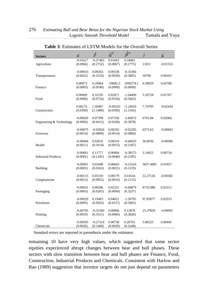
Table 3: Estimates of LSTM Models for the Overall Series

Standard errors are reported in parenthesis under the estimates.

remaining 10 have very high values, which suggested that some sector

equities experienced abrupt changes between bear and bull phases. These

sectors with slow transition between bear and bull phases are Finance, Food,

Construction, Industrial Products and Chemicals. Consistent with Harlow and

Rao (1989) suggestion that investor targets do not just depend on parameters

Sectors ̂ ̂ ˆU ˆU ̂ K̂

Agriculture

-0.01617

(0.0066)

-0.27463

(0.2732)

0.01693

(0.0067)

0.34681

(0.2775) 11811 -0.01553

Transportation

-0.00033

(0.0022)

0.09263

(0.2516)

0.00538

(0.0038)

-0.35384

(0.3805) 30706 0.00102

Finance

0.00073

(0.0005)

0.29964

(0.0540)

-59682.5

(0.0000)

1099274.1

(0.0000)

6.59829

0.05788

Food

0.00069

(0.0006)

0.32195

(0.0724)

0.02671

(0.0156)

-1.04499

(0.5662)

5.59728

0.01767

Construction

0.06174

(0.0390)

1.50487

(1.1489)

-0.06165

(0.0390)

-1.24419

(1.1565)

7.79795

-0.02434

Engineering & Technology

-0.00029

(0.0004)

0.07399

(0.0415)

0.07336

(0.0106)

-2.60672

(0.3878)

6791.84

0.02064

Footwear

-0.00075

(0.0014)

-0.03826

(0.0809)

0.00182

(0.0014)

-0.02295

(0.0860)

6573.63

-0.00843

Health

-0.00064

(0.0011)

0.02032

(0.1014)

0.00218

(0.0015)

-0.06033

(0.1367)

36.0036

-0.00060

Industrial Products

-0.00061

(0.0081)

0.11777

(0.1245)

0.00694

(0.0048)

-0.39575

(0.2395)

3.14922

0.00754

Building

-0.00001

(0.0001)

0.01698

(0.0163)

0.00643

(0.0031)

-0.21616

(0.1219)

3837.4081

0.01857

Conglomerate

-0.00115

(0.0013)

0.05310

(0.0952)

0.00179

(0.0014)

0.01634

(0.1115)

22.27126

-0.00382

Packaging

-0.00031

(0.0003)

0.06586

(0.0283)

0.02231

(0.0094)

-0.68879

(0.3237)

8735.088

0.02212

Petroleum

-0.00029

(0.0005)

0.19403

(0.0563)

0.04621

(0.0137)

-1.50791

(0.5065)

97.85877

0.02013

Printing

-0.00795

(0.0059)

-0.31560

(0.3511)

0.00866

(0.0060)

0.13878

(0.3826)

25.37859

-0.00695

Chemicals

-0.00595

(0.0026)

-0.27314

(0.1469)

0.00738

(0.0029)

0.26701

(0.1649)

5.86525

0.00445


computed with the distribution of market returns; there is no apparent

common value for this parameter across different industries.

Table 4: Estimates of LSTM Models for the period before the Global

Financial Crisis

NB: Standard errors are reported in parenthesis under the estimates.

The up-market betas for the sectors are recorded in the ˆU column, and 11 of

these are significant at 5% level. We can see that the LSTM model therefore

provide widespread support for time varying betas, with variations linked to

movements in the business cycle. Eight of the eleven statistically significant

up market betas are negative; this is in agreement with the literature that risk

in up market is lower than that in the down-markets.


Agriculture

0.07620

(0.0000)

3.84274

(0.0000)

-0.07594

(0.0000)

-3.63910

(0.0000)

1.12535

-0.04361

Transportation

0.00087

(0.0031)

0.08384

(0.4095)

0.00728

(0.0053)

-0.55269

(0.5785)

90.9997

0.00078

Finance

0.00281

(0.0009)

0.71890

(0.1383)

-0.00352

(0.0031)

-0.15970

(0.2666)

199036

0.00483

Food

0.00492

(0.0026)

0.89530

(0.2312)

-0.00669

(0.0048)

-0.27696

(0.3473)

5.44033

0.00064

Construction

-0.00048

(0.0009)

0.07480

(0.1362)

0.01335

(0.0056)

-0.27288

(0.3761)

240.8016

0.00851


0.00051

(0.0003)

0.05339

(0.0373)

0.00627

(0.0026)

-0.32555

(0.1441)

42.0485

0.01102

Footwear

0.00095

(0.0003)

-0.02572

(0.0418)

0.01281

(0.0082)

-0.49648

(0.3480)

317.25439

0.01759

Health

0.00181

(0.0007)

0.22437

(0.1132)

-0.00713

(0.0035)

0.20166

(0.2620)

47.52201

0.00669

Industrial Products

0.00081

(0.0007)

0.42974

(0.1017)

0.00943

(0.0054)

-0.78205

(0.3354)

32.37108

0.00973

Building

0.00008

(0.0001)

0.01019

(0.0098)

-0.00120

(0.0005)

0.05569

(0.0321)

62.89803

0.00945

Conglomerate

0.04737

(0.0611)

1.78521

(1.7901)

-0.04732

(0.0611)

-1.53001

(1.7883)

1.95266

-0.02696

Packaging

0.00024

(0.0001)

0.01070

(0.0129)

-0.00117

(0.0008)

0.05571

(0.00458)

28.86846

0.01048

Petroleum

0.00041

(0.0004)

0.23877

(0.0456)

2.12528

(0.6822)

-61.26900

(19.9732)

133.70077

0.03288

Printing

-0.01161

(0.0076)

-0.60131

(0.4854)

0.01445

(0.0078)

0.37268

(0.5117)

25.32094

-0.00732

Chemicals

-0.01035

(0.0052)

-0.48603

(0.2940)

0.01296

(0.0056)

0.47959

(0.3255)

4.38522

-0.00532



Table 5: Estimates of LSTM Models for the period after the Global Financial

Crisis

Note: Standard errors are reported in parenthesis under the estimates

We therefore divided the data into two sub-series with February 2008 as the

break point. We estimated LSTM model for each of the sub-series (before and

after financial crisis). The results are presented in Tables 4 and 5.


Agriculture

-0.02684

(0.0089)

-0.76943

(0.3669)

0.02768

(0.0089)

0.72447

(0.3745)

25.58852

-0.01500

Transportation

-0.00067

(0.0027)

0.15000

(0.2832)

-0.00521

(0.0072)

0.19578

(0.5435)

200978

0.00408

Finance

-0.00133

(0.0007)

0.04335

(0.0000)

0.01511

(0.0094)

-0.53924

(0.3887)

1168.939

0.01542

Food

-0.00013

(0.0008)

0.15647

(0.0840)

0.03739

(0.0148)

-1.33213

(0.5393)

8.54906

0.01754

Construction

0.10070

(0.0454)

2.17242

(1.3330)

-0.10198

(0.0454)

-2.01154

(1.3378)

15.89829

-0.12631


-0.00160

(0.0009)

0.05963

(0.0870)

0.08458

(0.0183)

-2.88614

(0.6501)

62.93592

0.02026

Footwear

-0.00100

(0.0013)

-0.02068

(0.0740)

0.00201

(0.0013)

-0.07444

(0.0803)

687.96581

-0.00813

Health

-0.01604

(0.10155)

-0.48717

(0.5253)

0.01541

(0.0155)

0.51464

(0.5286)

29.13244

-0.02288

Industrial Products

0.00409

(0.0053)

0.15798

(0.2379)

-0.00555

(0.0053)

-0.22344

(0.2477)

21.57934

-0.01217

Building

-0.00006

(0.0003)

0.02947

(0.0358)

0.01035

(0.0058)

-0.33675

(0.2217)

3777.230

0.01857

Conglomerate

-0.00309

(0.0029)

-0.11442

(0.1556)

0.00403

(0.0031)

0.00576

(0.1689)

10.01772

-0.00518

Packaging

-0.00097

(0.0006)

0.10910

(0.0622)

0.03559

(0.0172)

-1.03764

(0.5716)

9738.0865

0.02212

Petroleum

-0.00159

(0.0011)

0.11192

(0.1082)

0.09591

(0.0231)

-2.92724

(0.8223)

6076.0114

0.02065

Printing

0.11339

(0.0692)

3.14433

(2.0395)

-0.11640

(0.0692)

-3.11567

(2.0436)

15.79602

-0.02638

Chemicals

-0.00147

(0.0005)

-0.05384

(0.0482)

0.00763

(0.0037)

-0.21275

(0.1717)

9.30564

0.01033


In Table 4, the transition between bull and bear period is abrupt in most of the

portfolios. The speed is highest for financial sector and lowest for

conglomerates sector.

After the financial crisis (starting from March, 2008) when the stock market

started experiencing the global shock, we have similar results of LSTM

models in Table 5. We found that Packaging, Transportation, Petroleum and

Building experienced abrupt change between market phases. This implies that

these portfolios (industries) recovered fast after the crisis.

5.0 Policy Implications and Conclusion

Financial analysts believe that market and portfolio betas are influenced by

the alternating forces of bull and bear markets. Most of the studies have

applied simple threshold model which classifies market in these two phases.

This work is the first of its kind classifying Nigerian stock markets into bull

and bear phases using the logistic smooth threshold market (LSTM) model.

Using the All share Index (ASI) and selected 15 portfolios (sectors/industries

on Nigerian Stock Exchange), we tested for up (bull) and down (bear) markets

differentials using the logistic smooth transition nonlinearity test similar to

that proposed in Luukkonnen, et al. (1988) and applied in Teräsvirta (1994).

The results obtained showed strong evidence of betas varying between bull

and bear phases. The estimates of LSTM model indicated that the transition is

fast (abrupt) for most of the portfolios and this is in support of the

homogenous beliefs among the investors as a result of news/information

symmetry. Also, the up-market and down-market betas are significantly

different in most of the portfolios.

Our results are consistent with Pagan and Sossounov (2003) and Cunado et al.

(2008) who found stocks spending more time in bull-market than bear-market

states. This work has offered an alternative way of studying Nigerian stock

market asymmetries.

Findings of this research have policy implications. Within the period under

study, the CPM identified the Petroleum, Finance and Food to be of higher

risk as compared to aggregate market risk of all sectors. We also found that

for most industries, the beta estimate obtained before financial crisis is

different from that obtained after the financial crisis.



References

Aslanidis, N., Osborn, D.R. and Sensier, M. (2002). Smooth Transition

Regression Models in UK Stock Returns. Centre for Growth and

Business Cycle Research paper. pp. 1-32.

Akingunola, R. O. (2006). Capital Asset Pricing Model and Shares Value in

the Nigerian Stock Market. Journal of Banking and Finance, 8(2):64-

78.

Ang, A. and Bekaert, G. (2002). Regime Switches in Interest Rates. Journal of

Business and Economic Statistics 20:163–182.

Bello, A. I. and Adedokun, L. W. (2011). Empirical Analysis of the Risk-

Return Characteristics of the Quoted Firms in the Nigerian Stock

Market. Global Journal of Management and Business Research, 11(8)

Bhardwaj, R. and Brooks, L. (1993). Dual Betas from Bull and Bear Markets:

Reversal of the Size Effect. Journal of Financial Research, 16:269-83.

Chen, S. (1982). An Examination of Risk Return Relationship in Bull and

Bear Markets using Time Varying Betas. Journal of Financial and

Quantitative Analysis, 17:1-10.

Chan, F. and Theoharakis, B. (2009). Re-Parameterization of Multi-regime

STAR-GARCH Model. 18th World IMAS/MODSIM Congress.

Cairns, Australia. pp. 1384-1390. http://mssanz.org.au/modsim09.

Cohen, J. B., Zinbarg, E.D. and Zeikel, A. (1973). Investment Analysis and

Portfolio Management, Revised Edition (Homewood, IL: R. D. Irwin

Co., 1973).

Cohen, J. B., Zinbarg, E.D. and Zeikel, A. I. (1987). Investment Analysis and

Portfolio Management, 5th Edition (Homewood, IL: R. D. Irwin Co.

Cunado, J., Gil-Alana, L.A., Perez de Gracia, F. (2008). Stock Market

Volatility in US Bull and Bear Markets. Journal of Money, Investment

and Banking. Issue 1.


Dukes, W.P., Bowlin, O.D. and MacDonald S.S. (1987). The performance of

beta in forecasting portfolio returns in bull and bear markets using

alternative market proxies, Quarterly Journal of Business and

Economics 26:89-103.

Fabozzi, F.J. and Francis, J.C. (1977). Stability Tests for Alphas and Betas

over Bull and Bear Market Conditions. Journal of Finance, 32:1093–

1099.

Fabozzi, F. J. and Francis J. C. (1979). Mutual fund systematic risk for bull

and bear markets: An empirical examination, Journal of Finance

34:1243-1250.

Ferson, W.E. and Korajczyk, R. A. (1995), Do Arbitrage Pricing Models

Explain the Predictability of Stock Returns?, Journal of Business,

68:11-23.

Ferson, W.E. and Harvey, C.R. (1998). Fundamental determinants of national

equity market returns: A perspective on conditional asset pricing.

Journal of Banking and Finance 21:1625-1665

Gil-Alana, L.A., Shittu, O.I. and Yaya, O.S. (2014). On the Persistence and

Volatility in European, American and Asian Stocks Bull and Bear

Markets. Journal of International Money and Finance 40: 149-162.

Gitman, S. and Joehnk, M. D. (1996). Fundamentals of Investing. 6th

edition,

Harpercollins Publishing.

Granger, C.W. and Silvapulle, P. (2001). Large Returns, Conditional

Correlation and Portfolio Diversification: A Value-At-Risk Approach.

Institute of Physics Publishing, 1:542-51.

Granger, C.W.J. and Terasvirta, T. (1993). Modelling Nonlinear Economic

Relationships. Oxford: Oxford University Press. Chinese edition 2006:

Shanghai University of Finance and Economics Press.

Gonzalez, L., Powell, J.G., Shi, J. and Wilson, A. (2005). Two centuries of

bull and bear market cycles, International Review of Economics and

Finance 14:469-486.



Guidolin, M. and Timmermann, A. (2004). Economic Implications of Bull

and Bear Regimes in UK Stock and Bond Returns. Economic Journal,

115:111–143.

Gursakal, S. (2010). Detecting long memory in bulls and bears markets:

evidence from Turkey. Journal of Money, Investment and Banking.

Issue 18.

Hamilton, J. D. (1989). A New Approach to the Economic Analysis of Non-

stationary Time Series and the Business Cycle. Econometrica, 57:357–

384.

Hamilton, J.D. (1994). Time Series Analysis. Princeton University Press.

Hamilton, J.D. and Susmel, R. (1994). Autoregressive Conditional

Heteroskedasticity and Changes in Regime. Journal of Econometrics,

64:307–333.

Harlow, V.W. and Rao, R.K.S. (1989). Asset pricing in a generalized mean-

lower partial moment framework: theory and evidence. Journal of

Finance and Quantitative Analysis, 24:285-311.

Jagannathan, R. and Wang, Z. (1996). The Conditional CAPM and the Cross

Section of Expected Returns. Journal of Finance, 51:3-53.

Kandir, S.Y. (2008). Macroeconomic Variables, Firm Characteristics and

Stock Returns: Evidence from Turkey. International Research Journal

of Finance and Economics, Issue 16.

Kim, M.K. and Zumwalt, K.J. (1979). An Analysis of Risk in Bull and Bear

Markets. Journal of Financial and Quantitative Analysis, 14(5):1015-

1025.

Litner, J. (1965). The Valuation of Risk Assets and the Selection of Risky

Investments in Stock Portfolios and Capital Budgets. Review of

Economic Statistics, 47:13-37.


Leybourne, S., Newbold, P. and Vougas, D. (1998). Unit Roots and Smooth

Transitions. Journal of Time Series Analysis 191:83-97.

Luukkonen, R. Saikkonen, P. and Teräsvirta, T. (1988). Testing Linearity

against Smooth Transition Autoregressive models. Biometrika,

75:491-499.

Lunde, A. and Timmermann A. (2001). Duration Dependence in Stock Prices:

An Analysis of Bull and Bear Markets. Working Paper.

Maheu, J. and McCurdy, T. (2000). Identifying bull and bear markets in stock

returns. Journal of business and Economic Statistics, 18:100-112.

Maringer, D. and Meyer, M. (2008). “Smooth Transition Autoregressive

Models-New Approaches to the Model Selection Problem”. Nonlinear

Dynamical Methods and Time Series Analysis in Studies in Nonlinear

Dynamics and Econometrics, 121:1-21.

Olakojo, S. A and Ajide, K. B. (2010), Testing the Capital Asset Pricing

Model (CAPM): The case of the Nigerian Securities Market. Journal

of International Business Management. 4(4):239-242

Oludoyi, S. B. (2003). An Empirical Analysis of Risk Profile of Quoted Firms

in the Nigerian Stock Market. Ilorin Journal of Business and Social

Sciences, 8:9-19

Osamwonyi, I. O. and Asein, E. I. (2012). Market Risk and Returns: Evidence

from the Nigerian Capital Market. Asian Journal of Business

Management, 4(4):367-372.

Pagan, A. and Sossounov, K. (2003), A Simple Framework for Analyzing

Bull and Bear Markets. Journal of Applied Econometrics. 18:23-46.

Quandt, R. (1983) Computational problems and methods, in Z. Griliches and

M.D. Intriligator eds., Handbook of Econometrics I. Amsterdam:

Elsevier Science, pp. 699-746.

Schwert, G. W. (1989), Why Does Stock Market Volatility Change Over-

Time? Journal of Finance, 44:1115-1153.



Sharpe, W. F. (1964), Capital Asset Prices: A Theory of Market Equilibrium

under Conditions of Risk. Journal of Finance, 19(3):425 – 442

Teräsvirta, T. (1994). Specification, Estimation and Evaluation of Smooth

Transition Autoregressive Models. Journal of the American Statistical

Association, 89:208-218.

Turner, C. M., Richard S. and Charles R. N. (1989). A Markov Model of

Heteroskedasticity, Risk, and Learning in the Stock Market”, Journal

of Financial Economics, 25:3–22.

Wiggins, J.B. (1992), Betas in up and down Markets. The Financial Review,

27:107-123.

Woodward, G. and Anderson, H. M. (2009). Does Beta react to market

conditions? Estimates of bull and bear betas using a nonlinear market

model with an endogenous threshold parameter. Quantitative Finance,

9:913-924.

estimating bull and bear betas for the nigerian stock ... bull and bear betas... · 264 estimating...

Documents