Estimating Clustering Coefficients and Size of SocialNetworks via Random Walk

Stephen J. Hardiman∗Capital Fund Management,

Francehardimas@tcd.ie

Liran KatzirAdvanced Technology Labs,Microsoft Research, Israellirank@microsoft.com

ABSTRACTOnline social networks have become a major force in today’ssociety and economy. The largest of today’s social networksmay have hundreds of millions to more than a billion users.Such networks are too large to be downloaded or stored lo-cally, even if terms of use and privacy policies were to permitdoing so. This limitation complicates even simple computa-tional tasks. One such task is computing the clustering coef-ficient of a network. Another task is to compute the networksize (number of registered users) or a subpopulation size.The clustering coefficient, a classic measure of network con-nectivity, comes in two flavors, global and network average.In this work, we provide efficient algorithms for estimatingthese measures which (1) assume no prior knowledge aboutthe network; and (2) access the network using only the pub-licly available interface. More precisely, this work providesthree new estimation algorithms (a) the first external accessalgorithm for estimating the global clustering coefficient; (b)an external access algorithm that improves on the accuracyof previous network average clustering coefficient estimationalgorithms; and (c) an improved external access network sizeestimation algorithm.

The main insight offered by this work is that only a rela-tively small number of public interface calls are required toallow our algorithms to achieve a high accuracy estimation.Our approach is to view a social network as an undirectedgraph and use the public interface to retrieve a random walk.To estimate the clustering coefficient, the connectivity ofeach node in the random walk sequence is tested in turn.We show that the error of this estimation drops exponen-tially in the number of random walk steps. Another insightof this work is the fact that, although the proposed algo-rithms can be used to estimate the clustering coefficient ofany undirected graph, they are particularly efficient on socialnetwork-like graphs. To improve the network size prior-artestimation algorithms, we count node collision one step be-fore they actually occur. In our experiments we validateour algorithms on several publicly available social networkdatasets. Our results validate the theoretical claims anddemonstrate the effectiveness of our algorithms.

∗Research was conducted while the author was unaffiliated.

Copyright is held by the International World Wide Web ConferenceCommittee (IW3C2). IW3C2 reserves the right to provide a hyperlinkto the author’s site if the Material is used in electronic media.WWW2013, May. 13-17, Rio de Janeiro, BrazilACM 978-1-4503-2035-1/13/05.

Categories and Subject DescriptorsF.2.2 [Theory of Computing]: Analysis of Algorithmsand Problem Complexity—Nonnumerical Algorithms andProblems

General TermsAlgorithms

KeywordsEstimation, Sampling, Clustering Coefficient, Social Net-work

1. INTRODUCTIONThe popularity of online social networks has grown enor-

mously in recent years. Users of the most popular socialnetwork, FacebookTM, now number greater than a billion1.This popularity has increased interest in analyzing the prop-erties of these networks. In [2, 13, 21] the authors investigatestructural measures of online social networks, including de-gree distribution and clustering coefficient.

Large social networks, as well as search engines, providea public interface as part of their service. Estimating struc-tural measures of the network using only these public inter-faces is a research question that has received much attentionin recent studies. Search engine public interfaces have beenused in [6, 8] to estimate corpus size, index freshness, anddensity of duplicates, and in [7] estimate the impressionrankof a webpage. Online social network public interfaces havebeen used in [13, 14, 25] to estimate the assortativity co-efficient, degree distribution, and clustering coefficients ofonline social networks, as well as in [14, 15] to estimate thenumber of registered users.

In practical scenarios, the underlying social network maybe available only through a public interface. The publicinterface of most social networks provides the ability to re-trieve a list of a user’s connections (“friends”). By applyingthis function iteratively to a random member of the connec-tion list one can effectively perform a random walk on thenetwork. Although the public interface allows us to store thesocial network locally, this practice is considered impracti-cal due to high time/space/communication cost and oftenviolates the terms of use agreement. In light of this, in thispaper we proceed under the assumption that (1) only ex-ternal access to the social network is available; and (2) onlya small number of users/nodes can be sampled. The main

1http://newsroom.fb.com/News/457/One-Billion-People-on-Facebook

539

insight offered by this work is that, even under these limita-tions, our algorithms achieve a good estimation accuracy ofthe network’s structural measures.

This work focuses on two particular structural measures.The first measure is called the clustering coefficient. The sec-ond measure is the size of the network. Namely, the numberof registered users in the network2.

The clustering coefficient comes in two main flavors, (1)the network average clustering coefficient [12]; and (2) theglobal clustering coefficient [12]. Both measures are impor-tant for the understanding of the network structure. First,we introduce the local clustering coefficient of a node in agraph as the ratio of the number of edges between its neigh-bors to the maximal possible number of such edges. Thenetwork average clustering coefficient of a graph is the localclustering coefficient averaged over the set of nodes in thegraph. The global clustering coefficient of a graph is theratio of the number of triangles (ordered triples of differ-ent nodes in which are all nodes connected) to the numberof connected triplets (ordered triples of different nodes inwhich consecutive nodes are connected).

The size of the network is one of the basic structural mea-sures. The network size can determine the worth of a net-work (for business development). For certain applicationsin business development and advertisement, the size of asocial network subpopulation is extremely important. Forexample, the number of users of an online product or thenumber of potential users for a product. The subpopulationfraction (which can also be estimated efficiently [15]) andthe network size can determine the size of the subpopula-tion. Although some networks report their size periodically,the difference between consecutive reports can be more thanten percent. Moreover, even if this number is reported everyday, an unbiased independent estimate would be beneficial.

This work contains three main contributions. The firstand principal contribution is the first external access esti-mator for the global clustering coefficient. The second con-tribution is an improved external access estimator for thenetwork average clustering coefficient. The third contribu-tion is an improved external access estimator for the networksize.

The rest of this paper is organized as follows. Section 2surveys related work. Section 3 provided preliminaries andnotations. Section 4 details our clustering coefficient estima-tors. Section 5 details our network size estimator. Section 6reports our experimental results. We conclude the paper inSection 7.

2. BACKGROUND AND PRIOR WORKWe consider the social network as an undirected graph

where nodes and edges are represented by users and friend-ship connections. Although the algorithms presented in thispaper are correct for general graphs, the structure of socialnetworks renders them even more effective.

Both the network average and the global clustering coeffi-cient (also known as transitivity) are a long studied classicalcomputer science problem. The running time of the naivealgorithm for computing them is O(n3) for dense graphs(where n is the number of nodes in the graph), and it is con-sidered impractical for large graphs. For the global cluster-

2Technically, the algorithm estimates the size of the largestconnected component and isolated users are neglected.

ing coefficient, the most challenging part of the computationis counting the total number of triangles, since computingthe number of connected triplets is done in linear time. Tothis end, the computation of global clustering coefficient andthe computation of the number of triangles is equivalent.

We provide references for a partial list (most recent) forseveral directions for estimating the number of triangles.Alon et al. [3] provided an exact algorithm for the count-ing the number of triangles. The running time of this al-

gorithm is O(E2ω

ω+1 ) = O(E1.41), where ω < 2.376 is theexponent of matrix multiplication. Avron [4] provided anestimator based on numerical matrix-vector multiplicationusing O(log2 n) samples, each of which requires O(|E|) time(where E is the set of nodes in the graph). Both these algo-rithm access the entire graph.

Buriol et al. [10] provided an approximate solution to theglobal clustering coefficient in the streaming model. Thestreaming models allows the algorithm to have a single passon the input while (1) reading the edges in arbitrary/vertexordered appearance (different algorithms) and (2) use con-stant amount of space. Becchetti et al. [9] provided analgorithm for the network average clustering coefficient inthe streaming model. In contrast to [3, 4] these works as-sume there is no random access to the graph. However, thestreaming algorithms access each edge at least once.

Schank et al. [27], provided estimators for both the globaland network average clustering coefficient which only usesa sample of the nodes. However, unlike our work, the al-gorithms assume there is an efficient way to sample nodeswith distribution that is tailored to the clustering coefficient.Specifically, for the network average clustering coefficient thesampling distribution is the uniform distribution and for theglobal clustering coefficient each node vi with degree di issampled proportionally to di(di − 1). In contrast, the algo-rithms provided in this work do not even assume the numberof nodes is known and does not require a tailored samplingdistribution.

Another research direction [13, 25] addresses the problemof estimating the local clustering coefficient with externalaccess3. In these papers, the graph can only be accessedvia the exploration of nodes that lie on the frontier of previ-ously explored nodes. Ribeiro et al [25] explored the graphusing a random walk. Gjoka et al. [13] explored the graphusing Metropolis-Hastings random walk that generates uni-form samples from the nodes set. In both these papers, thecomputation requires augmenting the set of explored nodes,S, with further exploration of S’s ego network. An ego net-work of a set of users S, is the set of users S′ that containsall the users in S and all their (immediate) friends [13, 28].

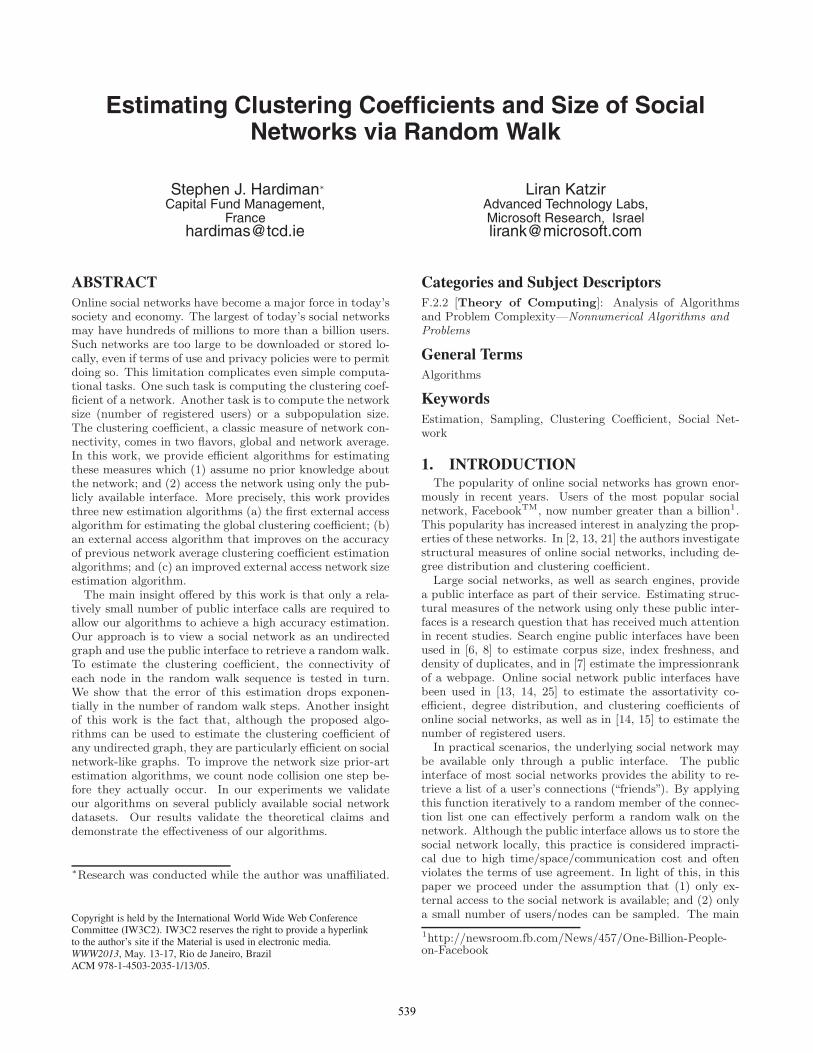
In this work, we perform a random walk but remove therequirement of exploring the ego network. This differenceis illustrated in Figure 1. The random walk contains threenodes v1, v2, v3. Our approach requires the exploration ofthe nodes v1, v2, v3 (marked by a thick circle), the ego net-work approach requires additional exploration of the nodesv4, v5, v6. In total the ego network requires exploration ofall the nodes v1, v2, . . . , v6 (marked by solid fill). In sec-tion 6, we show that the algorithm provided in this paper

3Ref [25] mistakenly refers to the global clustering coeffi-cient, but provides an accurate definition of the networkaverage clustering coefficient.

540

va

vb

vc

in random walk

in ego network

beyond reach

visible by random walkand ego network

visible by ego networkonly

visible by neither

v1 v2

v3

v4

v5

v6

v7

v8

v9

Figure 1: An example of a random walk with itscorresponding ego network augmentation.

outperform competing approaches [25, 13] on all the socialnetworks we study.

Another method for estimating the clustering coefficientfrom a random walk was presented in [14]. This algorithmuses only the ids of nodes visited by a random walk anddoes not assume any prior information. In contrast, the al-gorithms in this paper assume not only the node ids arevisible, but also their list of friends (adjacency list). Practi-cally, if this assumption holds, it renders [14] uncompetitive.

In this work, two estimators are provided for the cluster-ing coefficient. The first for the network average clusteringcoefficient and the second for the global clustering coeffi-cient. Both estimators use samples taken from a randomwalk on the graph. Namely, not only that the algorithms donot access the entire graph, they do not even have randomaccess to the graph’s nodes and edges. The only assumptionis that a random walk can be performed via the public inter-face, and the visited node ids along with their list of friends(adjacency list). This is the case for many social networks.Indeed, the act of performing a random walk at all in anonline social network typically necessitates having access tothis information.

Both [14, 15] provide estimators for the total number ofregistered users in the network. These algorithms use onlythe node ids visited on the random walk and do not assumeany prior information on the graph. The underlying ideain both papers is to count node collision, a pair of indices(k, l) such that the same node appears in the kth and lth

location of the random walk. Nodes on the random walkare highly correlated when their index distances (|k − l|) areshort, which increases the probability of a node collision. Toensure a unified probability of collision across all node pairs,a collision is counted only if the nodes appear a significantnumber of steps apart. These works differ in the way theyselect these pairs. In [15] the estimator chooses all pairsin which both k and l are a multiple of a parameter m,while [14] chooses all pairs in which m ≤ |k − l|. Choosingall pairs [14] is practically better, but harder to analyze. Theconvergence of social network like graphs is very fast anddepends on the degree distribution. For example, if the nodedegrees are distributed according to a Zipfian distributionwith maximum degree of

√n and parameter α = 2, then the

number of samples needed to guarantee convergence for afixed accuracy is O(n1/4 log n) [15].

In some applications the size of a subpopulation needsto be estimated. This subpopulation is defined by a prop-erty of the user’s profile. For example, the number of regis-tered users who use a specified online product. Estimatingthe size of a subpopulation requires multiplying the totalsize of the network by the ratio the target nodes to thetotal nodes which could also be estimated by the randomwalk [15]. In this work, we improve the network size estima-tion algorithms by using not only the visited node ids, butalso the adjacency list of each of the visited nodes. This isdone by counting node collision one step before they actu-ally occur. Namely, two nodes on the random walk (enoughnodes apart) that share a connection. We call this collisiona neighbor collision.

3. PRELIMINARIES AND NOTATIONSWe denote by G(V, E) the social network’s underlying

undirected graph, where V = {v1, v2, . . . , vn} is the set ofnodes (users) and E is the set of edges (friendship connec-tions). Additionally, we denote by di the degree of nodevi and the sum of degrees by D =

∑ni=1 di = 2 |E|. The

maximum degree of a node in the graph is noted by dmax =maxn

i=1 di.We denote by an n×n matrix A the adjacency matrix for

graph G. Namely, Ai,k = Ak,i = 1 if node vi is connectedby an edge to node vk and 0 otherwise. We assume no selfloops, thus Ai,i = 0 for all i.

Definition 1. A triplet of nodes (vj , vi, vk) is called con-nected if vj is connected to vi, vi is connected to vk, andj < k. Formally, if Aj,i = 1, Ai,k = 1, and j < k.

Definition 2. A triangle is a connected triplet (vj , vi, vk)in which vj and vk are connected. Formally, if Aj,k = 1.

Following these definitions, a triplet of nodes is connectedif j < k and Aj,iAi,k = 1 and it is a triangle if j < kand Ai,jAi,kAj,k = 1. For a specific node vi, the numberof connected triplets (vj , vi, vk) is thus

∑j<k Aj,iAi,k. Note

that∑

j<k Aj,iAi,k = di(di−1)/2 since there are di(di−1)/2choices for j < k in which both Aj,i = 1 and Ai,k = 1.For a specific node vi, the number of (vj , vi, vk) triangles isdenoted by li =

∑j<k Ai,jAi,kAj,k (it is also the number of

edges between neighbors of vi) .

Definition 3. The local clustering coefficient [12] for nodevi, denoted by ci, is defined as the ratio of the number of(vj , vi, vk) triangles to the number of (vj , vi, vk) connectedtriplets. Formally,

ci =2li

di(di − 1)

Note that ci ∈ [0, 1]. In the case where di = 1 or di = 0, wehave ci = 0.

Definition 4. The network average clustering coefficient[12], denoted by cl, is defined by

cl =1

n

n∑i=1

ci

541

Definition 5. The global clustering coefficient [12], de-noted by cg, is defined as the ratio of the total number oftriangles to the total number of connected triplets. Formally,

cg =2∑n

i=1 li∑ni=1 di(di − 1)

Note that a set of three nodes {vj , vi, vk} forms three dif-ferent triangles4 one is counted in lj , a second in li, and athird in lk.

The first step of the estimation algorithms is to generatea random walk. A random walk with r steps on G, denoteby R = (x1, x2, . . . , xr), is defined as follows: start from anarbitrary starting node vx1 , then move to one of the neigh-boring nodes uniformly at random (with probability 1

dxi)

and repeat r − 1 times. We use Pr [A] to denote the prob-ability that event A occurred. We denote the distributioninduced by R, as

πR = (Pr [xr = 1] ,Pr [xr = 2] , . . . ,Pr [xr = n]) .

The probability Pr [xr = i] after many random walk steps

converges to pi � di/D and the vector π = (p1, p2, . . . , pn)is called the stationary distribution of G.

In our estimators, we assume that x1 is drawn from thestationary distribution5. This assumption is valid becausewe can always perform an initial random walk from an ar-bitrary node to draw a starting node from the stationarydistribution.

The actual number of steps needed to converge to thestationary distribution depends on the mixing time of G.There are several definitions of mixing time, many of whichare known to be equivalent up to constant factors. All def-initions take an ε parameter to measure the distance be-tween the stationary and the induced distribution. Boththe book [17] and the survey [19] provide excellent overviewon random walks and mixing times. We denote the mixingtime of graph G by τ (ε) or τ (ε is assumed to be a smallconstant). We use the following definition:

Definition 6. Let R = (x1, x2, . . . , xr) be a random walk.Then, let the distance between π and πR be the maximum dif-ference between the probability of drawing a specific node xr

over all possible choices of nodes x1 and xr. Namely,

d(r) =n

maxx1=1

nmaxi=1|pi − Pr [xr = i]|.

We have τ (ε) = min {r | d(r) ≤ ε}.Social network graphs are known to have low mixing times

and constant clustering coefficients (which are not extremelysmall). Recently, Addario-Berry et al [1] proved rigorouslythat the mixing time of Newman-Watts [23, 24] small worldnetworks is Θ(log2 n). Mohaisen et al. [22] provide numeri-cal evaluation of the mixing time of several networks. Theauthors claim that “the mixing time is much larger than an-ticipated”. However, Table 1 and Figure 2 in their papershow that to have d(r) ≈ 0, the number of steps should

4In some references a triangle is defined by an unordered setof three nodes, in which case cg is defined by three times theratio of the total number of triangles to the total number ofconnected triplets.5This is not necessary in practice. However, the runningtime bound is tighter with this assumption.

be r = log2 n for the Facebook network, r = 3 log2 n forthe DBLP and youtube networks, and r = 10 log2 n for theLive Journal network. Both the low mixing time and therelatively high value of the clustering coefficients enable theclustering coefficient estimation algorithms in this paper toprovide accurate result with relatively low number of sam-ples. Notations are summarized in Table 1.

G underlying undirected graphn number of nodes in the graphA adjacency matrix for Gvi node in Gdi degree of node viD the sum all nodes degrees

∑ni=1 di

r total number of steps in the random walkxk the index of kth node in the random walk

pi p(xk = i) = diD

π the stationary distribution (p1, p2, . . . , pn)li number of edges between neighbors of vicl network average (local) clustering coefficientcg global clustering coefficientcl cl estimationcg cg estimationn n estimation

τ (ε) mixing timedmax maxn

i=1 di

Table 1: Summary of notations

4. CLUSTERING COEFFICIENT ESTIMA-TION

We now present the main observation used in both net-work average and global clustering coefficient estimators.Given a random walk (x1, x2, . . . , xr), we define a new vari-able φk = Axk−1,xk+1 for every 2 ≤ k ≤ r − 1. For any

function f(xk) the following holds6:

E [φkf(xk)] =n∑

i=1

piE [φkf(xk)|xk = i]

=

n∑i=1

diD

2lid2i

f(vi) (1)

=

n∑i=1

1

D

2lidi

f(vi).

The first equality holds due to the law of total expectation.The second equality holds because there are d2i equal proba-bility combinations of (xk−1, vi, xk+1) out of which only 2liform a triangle (vj , vi, vk) or a reverse triangle (vk, vi, vj).Notice that in a triangle or a reverse triangle vj is connectedto vk (Aj,k = 1). The third equality holds due to algebraicmanipulation.

4.1 Network average clustering coefficientTo estimate cl, we introduce two variables. First, we de-

fine Φl as a weighted sum of φjs, Φl =1

r−2

∑r−1k=2 φk

1dxk−1

.

Second, we define Ψl as the sum of the sampled nodes re-ciprocal degrees, Ψl =

1r

∑rk=1

1dxk

.

6We choose f(vi) = 1/ (di − 1) for the network average clus-tering and f(vi) = di for the global clustering estimator.

542

Using linearity of expectation and Eq (1) it is easy tocompute Φl and Ψl expectation.

E [Φl] = E

[φk

1

dxk − 1

]=

n∑i=1

1

D

2lidi(di − 1)

=1

D

n∑i=1

ci

E [Ψl] = E

[1

dxk

]=

n∑i=1

diD

1

di=

n

D

From the above equations we can isolate cl and get that:

cl =1

n

n∑i=1

ci =E [Φl]

E [Ψl]

Intuitively, both Φl and Ψl converge to their expected valuesand the estimator Φl/Ψl converges to cl as well.

Definition 7. Let cl be the estimator for cl, defined asfollows:

cl �Φl

Ψl.

Lemma 1. For any ε ≤ 1/8 and δ ≤ 1 we have:

Pr[cl(1− ε) ≤ cl ≤ cl(1 + ε)] ≥ 1− δ

when the number of samples, r, satisfies:

r ≥ rl ∈ O

(D

nclτ (ε)

).

Proof. The proof first finds the number of step, rl, whichguarantees both Φl and Ψl be within ε/3 approximations totheir expected values with probability at least 1− δ/2. SeeAppendix A for more details. Since the probability of Φl orΨl deviating from their expected value is at most δ/2, theprobability of either Φl or Ψl deviating is at most δ (usingthe union bound). Then, we use the fact that

(1− ε)cl ≤(1− ε

3)

(1 + ε3)

E [Φl]

E [Ψl]≤ Φl

Ψl≤ (1 + ε

3)

(1− ε3)

E [Φl]

E [Ψl]≤ (1+ ε)cl

to complete the proof.

Note that for social network like graph the mixing time isassumed to be relatively low (for Newman-Watts networksτ (ε) = O(log2 n) [1]), D = O(n) and cl is a small constant.Thus, the number of steps needed is linear in the mixingtime, τ (ε).

4.2 Global Clustering CoefficientTo estimate cg, we introduce two variables. First, we de-

fine Φg as a weighted sum of φjs, Φg = 1r−2

∑r−1k=2 φkdxk .

Second, we define Ψg as the sum of the sampled nodes de-grees minus one, Ψg = 1

r

∑rk=1 dxk − 1.

Using linearity of expectation and Eq (1) it is easy tocompute Φg and Ψg expectation.

E [Φg ] = E [φkdxk ] =n∑

i=1

1

D

2lidi

di =1

D

n∑i=1

2li

E [Ψg] = E [dxk − 1] =

n∑i=1

diD

(di − 1) =1

D

n∑i=1

di(di − 1)

From the above equations we can isolate cg and get that:

cg =1∑n

i=1 di(di − 1)

n∑i=1

2li =E [Φg ]

E [Ψg].

Intuitively, both Φg and Ψg converge to their expectedvalues and the estimator Φg/Ψg converges to cl as well.

Definition 8. Let cg be the estimator for cg, defined asfollows:

cg � Φg

Ψg.

Lemma 2. For any ε ≤ 1/8 and δ ≤ 1 we have:

Pr[cg(1− ε) ≤ cg ≤ cg(1 + ε)] ≥ 1− δ

when the number of samples, r, satisfies:

r ≥ rg ∈ O

(Ddmax

cg∑n

i=1 di(di − 1)τ (ε)

).

The proof is similar to the proof of Lemma 1, except thenumber of steps rg that guarantees convergences for Φg andΨg is different. See Appendix B for more details.

Both estimators presented in this section are consistent.Formally, as the number of samples, r, grows the estimatorsconverge to the true value. This also implies the estimatorsare asymptotically unbiased.

5. NETWORK SIZE ESTIMATIONIn this section we present an estimator for the graph size

(number of nodes). The estimator uses observations of nodepairs which are “far away” from each other in the randomwalk (as in Ref [14]). This assumption is needed to ensureboth nodes in a pair are (approximately) uncorrelated: eachdrawn from the stationary distribution7. Specifically, the es-timator examines node pairs whose index distance is greaterthan a threshold m. Formally,

I = {(k, l) | m ≤ |k − l| ∧ 1 ≤ k, l ≤ r} .The estimator counts weighted neighbor collisions. A neigh-

bor collision is a pair of indices (k, l) such that vxk and vxl

share a common neighbor. Formally, let Ai be the set of ver-tices adjacent to vi. Thus, Ai∩Aj is the set of nodes neigh-boring both vi and vj . Given a random walk (x1, x2, . . . , xr),we define a new variable φk,l = |Axk ∩Axl |. Note that if(k, l) ∈ I , then

E

[φk,l

1

dxkdxl

]=

n∑i=1

n∑j=1

diD

djD|Ai ∩Aj | 1

didj=

n∑j=1

(djD

)2

.

To see why∑n

i=1

∑nj=1 |Ai ∩Aj | = ∑n

j=1 d2j consider the

following combinatorial proof. For a node vk, the number ofconnected triplets (vi, vk, vj) with no restrictions on i andj is d2k. Thus, the total number of connected triplets is∑n

k=1 d2k. Alternatively, for nodes vi and vj the number

of connected triplets (vi, vk, vj) is |Ai ∩Aj |. Thus, the to-tal number of connected triplets can also be expressed by∑n

i=1

∑nj=1 |Ai ∩Aj |.

Next, we define Φn to be the averaged value of φk,l1

dxkdxl

over all possible choices of (k, l) ∈ I . Namely,

Φn =1

|I |∑

(k,l)∈Iφk,l

1

dxkdxl

.

7The larger the value of m, the smaller the bias in the esti-mate introduced by this correlation, but increasing m meansfewer observations of node pairs and a larger estimator vari-ance. However, note that we again benefit from the fast-mixing nature of social graphs, and m need only be of theorder O(log2 n).

543

Let Ψn be the averaged sum ofdxkdxl

over all possible choices

of (k, l) ∈ I . Formally,

Ψn =1

|I |∑

(k,l)∈I

dxk

dxl

.

Due to linearity of expectation, we have

E [Φn] = E

[φk,l

1

dxkdxl

]=

n∑j=1

(djD

)2

E [Ψn] = E

[dxk

dxl

]=

n∑i=1

n∑j=1

diD

djD

djdi

= nn∑

j=1

(djD

)2

Notice that n = E [Ψn]/E [Φn]. Intuitively, both Ψn andΦn converge to their expected values and the estimator Ψn/Φn

converges to n as well.

Definition 9. Let n be the estimator for n, defined asfollows:

n � Ψn

Φn.

Prior art algorithm [14, 15] count the number of nodecollisions, C, and estimates n by Ψn/C. A node collisionis a pair of indices (k, l) such that such that xk = xl. Incontrast Φn counts neighbor collision and estimates n byΨn/Φn.

Lemma 3. The neighbor collision estimator, n (defini-tion 9), has confidence intervals tighter than the node colli-sion estimator.

Proof. Formally, C = 1|I|

∑(k,l)∈I 1xk=xl where 1xk=xl

is 1 if xk = xl and 0 otherwise. The key observation is that

E[1xk+1=xl+1 | xk, xl

]= φk,l

1

dxkdxl

.

This stems from the combinatorial argument that (a) thereare dxkdxl equally likely joint node transitions from xk andxl to xk+1 and xl+1; and (b) in only φk,l = |Axk ∩Axl | ofthem xk+1 = xl+1 holds. Note that, xk is uncorrelated withxl when (k, l) ∈ I . Using this observation we have,

Φn =1

|I |∑

(k,l)∈IE[1xk+1=xl+1 | xk, xl

].

This is the Conditional Monte Carlo estimator8 of C, whichguarantees Var [C] ≥ Var [Φn] [26](Section 5.4).

5.1 Implementation notesThe straight forward computation of Ψn and Φn running

time is O(r2) and O(r2d2max) respectively. However, a care-ful implementation can reduce this complexity to O(r) andO(rdmax) respectively. For Φn the expected running can be

reduced to O(r∑n

i=1

d2iD).

First, we define (l+m)+ to be min {r, l +m} and (l−m)−

to be max {l −m, 1}. For the computation of Ψn instead ofmultiplying the value of 1

dxlby each dxk separately, it is mul-

tiplied by the sum of∑(l+m)+

k=(l−m)− dxk . The sum in turn, can

8Note that if (k, l) ∈ I , then (k − 1, l − 1) ∈ I except fork = 1 which holds only for a negligible fraction of the pairs.

be efficiently computed for every k in O(1), using a cumu-lative sum precomputation. Specifically, if Bq =

∑qk=1 dxk ,

then

|I |Ψn =r∑

l=1

1

dxl

(Br −B(l+m)+ +B(l−m)−

).

To compute Φn one must first construct an inverted indexof neighboring nodes. In document-term view, each node isa document containing adjacent nodes as terms. Specifi-cally if vj is a neighbor of xk then k is a term in vj . Therunning time of creating an inverted index is linear in the

number of terms (O(rdmax) worst case and O(r∑n

i=1d2iD) ex-

pected). Then, the entry for vj holds a list Lj of all indicesin which vj is a neighbor. Thus, |I |Φn =

∑nj=1 Cj , where

Cj =∑

(k,l)∈I|k∈Lj∧l∈Lj

1dxk

dxl. To efficiently compute Cj

in O(|Lj |), a precomputation Bq(j) =∑

q≥k∈Lj

1dxk

should

be used (similarly to the computation of Ψn).

6. EXPERIMENTAL EVALUATION

6.1 Networks with public datasetWe demonstrate the effectiveness of the estimators by

experimenting with social networks with known structure.Datasets statistics are enclosed in Table 2.

Network n D/n cl cgDBLP 977,987 8.457 0.7231 0.1868Orkut 3,072,448 76.28 0.1704 0.0413Flickr 2,173,370 20.92 0.3616 0.1076

Live Journal 4,843,953 17.69 0.3508 0.1179

Table 2: Networks statistics

In all our datasets we perform the following: (1) if the orig-inal network is directed, the direction is removed (the edge ismade undirected); (2) only the network’s largest connectedcomponent is retained and the rest of the nodes/users aredropped. All the datasets we use are publicly available9.

DBLP In the “Digital Bibliography and Library Project”(DBLP[18]) dataset each entry is a reference to a paperwhich contains a title and a list of authors. In thecorresponding network each node is an author and anedge between two authors represent co-authorship ofone or more papers. We used a snapshot taken Oct 01,2012.

Orkut Orkut is a general purpose social network. Thedataset contains a partial snapshot (11.3% of the nodes)taken during 2006 by [21]. In this social network thefriendship connections (edges) are undirected.

Flickr Flickr is an online social network with focus on photosharing. The dataset contains a partial snapshot takenduring 2006–2007 by [20]. In this social network thefriendship connections (edges) are directed.

9The DBLP, Orkut, Flickr, and LiveJournal are pub-licly available at http://dblp.uni-trier.de/xml/ andhttp://konect.uni-koblenz.de/networks/{orkut-links,flickr-growth,soc-LiveJournal1} [16], respectivly.

544

LiveJournal LiveJournal is an on-line social network withfocus on journals and blogs. The dataset contains apartial snapshot of the nodes taken by [5]. In thissocial network the friendship connections (edges) aredirected.

The x-axis in our figures is the percentage of mined nodes(number of mined nodes over the total number of networknodes). The y-axis is the relative estimated value (esti-mate value over the true value). We display [5%, 95%]-confidence intervals for all figures. A [5%, 95%]-confidenceinterval of random variable z, is defined as the interval [L, U ]such that Pr [z ≤ L] = 0.05 and Pr [z ≤ U ] = 0.95. Thus,Pr [z ∈ [L,U ]] = 0.9. To estimate the confidence interval,each simulation was run independently 100,000 times. Thevalues L and U are estimated by the 5th and 95th percentilevalues respectively.

In subsections 6.2 and 6.3 we compare the prior art al-gorithms method with the random walk approach describedin this work. For comparison we consider the following ap-proaches: (1) the estimator based on random walk combinedwith ego network exploration described in [25] (labeled RWEgo network); and (2) the estimator based on Metropolis-Hastings sampling with ego network exploration describedin [13] (labeled MH Ego Network). The estimator describedin subsection 4.1 is labeled random walk. In the randomwalk estimator (our approach) the number of mined nodes isexactly the random walk’s length, while in the Ego networkalgorithms (prior art) the mined nodes include the (sampled)walk nodes as well as their neighbors.

In subsection 6.4 we compare prior art node collision esti-mator [14, 15] (labeled node collision) with the new proposedneighbor collision estimator (labeled neighbor collision).

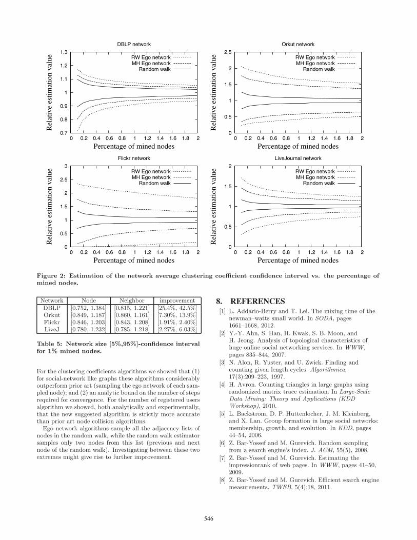
6.2 Network average clustering coefficientFigure 2 displays confidence intervals for all algorithms

and datasets. The proposed random walk estimator sig-nificantly outperforms ego network estimators. Specifically,using only 1% of the network size, the confidence intervalsof the random walk estimator are about fifty percent tighterfor the DBLP network and four times as tight for the Orkut,Flickr, and LiveJournal networks. The exact numbers areenclosed in Table 3.

Network random walk MH Ego RW EgoDBLP [0.967, 1.033] [0.942, 1.051] [0.910, 1.073]Orkut [0.916, 1.085] [0.583, 1.468] [0.426, 1.658]Flickr [0.891, 1.111] [0.557, 1.415] [0.064, 2.023]LiveJ [0.951, 1.054] [0.816, 1.200] [0.645, 1.329]

Table 3: Network average clustering [5%,95%]-confidence interval for 1% mined nodes.

6.3 Global clustering coefficientIn this subsection there is no prior art algorithm for com-

parison. To have a baseline, we retrofit the ego network es-timator for computing the global clustering coefficient. Theglobal clustering coefficient can be viewed as a weighted sumof local clustering coefficients. The ego network sampling es-timators multiplies each observed cxk by wk = dxk(dxk − 1)and divide the total by the sum W =

∑k wk.

Figure 3 displays confidence intervals for all algorithmsand datasets. The proposed random walk estimator sig-

nificantly outperforms ego network estimators by an evengreater margin when compared with the network averageclustering coefficient estimators. The curve for metropolishasting ego network in missing in the Flickr graph becauseall the values are greater than 8, which demonstrate theestimator’s inefficiency. In the LiveJournal graph, one cansee the upper 95% curves are even increasing. These curvesconverge only after 5% of the network is sampled. Usingonly 1% of the network size, the confidence intervals of therandom walk estimator are about three times tighter for theDBLP network and ten times tighter for the Orkut network.The ego network estimators for the Flickr and LiveJournalnetworks are extremely inaccurate in the [0.1%, 2%] range.The exact numbers are enclosed in Table 4.

Network random walk MH Ego RW EgoDBLP [0.869, 1.180] [0.659, 1.919] [0.609, 1.485]Orkut [0.892, 1.130] [0.424, 2.711] [0.317, 3.068]Flickr [0.922, 1.078] [0.212, 10.07] [0.176, 1.588]LiveJ [0.620, 1.523] [0.235, 4.275] [0.246, 3.051]

Table 4: Global clustering [5%,95%]-confidence in-terval for 1% mined nodes.

6.4 Network sizeIn this subsection we compare the node collision and neigh-

bor collision estimators. In all estimators the number ofmined nodes is exactly the random walk’s length. We usedm = 2.5%r as the separation parameter for all estimators.Namely, we used about 95% of the maximum number of(k, l) pairs (|I | ≈ 0.95r2). In Figure 4 we see that the neigh-bor collision estimator outperforms the node collision esti-mator. The node collision estimator and neighbor collisionestimator are Ψn/C and Ψn/Φn respectively. The perfor-mance of the estimators depend on the variance of Ψn, C,and Φn. The performance of the neighbor collision reducesthe variance of one factor, but retains the variance of Ψn.Therefore, we see a different performance impact on thesedatasets. Moreover, the fact that 1

1±x≈ 1∓x+x2∓· · ·+x2k

explains why the neighbor collision estimator has a greaterimpact on performance in the early stages of convergencewhen r is small.

Using only 1% of the network size, there was a significantaccuracy improvement in the DBLP network, a noticeableimprovement for the Orkut network, and negligible improve-ment for the Flickr and LiveJ networks. The exact numberare enclosed in Table 5. The second column is prior artnode-collision estimator; the third column is the proposednew neighbor collision estimator; and the fourth column isthe confidence bound improvement10.

7. CONCLUSIONSWe presented algorithms for estimating the (1) network

average clustering coefficient; (2) global clustering coeffi-cient; and (3) the number of registered users. These algo-rithms use the information collected by randomwalk, namely,the ids of the visited nodes along with their adjacency list.

10In the DBLP network the change from 1.384 to 1.221 in the95% confidence implies a (0.384−0.221)/0.384 improvementand the change in the 5% confidence from 0.752 to 0.815implies a (0.815 − 0.752)/(1 − 0.752) improvement.

545

0.7

0.8

0.9

1

1.1

1.2

1.3

0 0.2 0.4 0.6 0.8 1 1.2 1.4 1.6 1.8 2

Rel

ativ

e es

timat

ion

valu

e

Percentage of mined nodes

DBLP network

RW Ego networkMH Ego network

Random walk

0

0.5

1

1.5

2

2.5

0 0.2 0.4 0.6 0.8 1 1.2 1.4 1.6 1.8 2

Rel

ativ

e es

timat

ion

valu

e

Percentage of mined nodes

Orkut network

RW Ego networkMH Ego network

Random walk

0

0.5

1

1.5

2

2.5

3

0 0.2 0.4 0.6 0.8 1 1.2 1.4 1.6 1.8 2

Rel

ativ

e es

timat

ion

valu

e

Percentage of mined nodes

Flickr network

RW Ego networkMH Ego network

Random walk

0

0.5

1

1.5

2

0 0.2 0.4 0.6 0.8 1 1.2 1.4 1.6 1.8 2

Rel

ativ

e es

timat

ion

valu

e

Percentage of mined nodes

LiveJournal network

RW Ego networkMH Ego network

Random walk

Figure 2: Estimation of the network average clustering coefficient confidence interval vs. the percentage ofmined nodes.

Network Node Neighbor improvementDBLP [0.752, 1.384] [0.815, 1.221] [25.4%, 42.5%]Orkut [0.849, 1.187] [0.860, 1.161] [7.30%, 13.9%]Flickr [0.846, 1.203] [0.843, 1.208] [1.91%, 2.40%]LiveJ [0.780, 1.232] [0.785, 1.218] [2.27%, 6.03%]

Table 5: Network size [5%,95%]-confidence intervalfor 1% mined nodes.

For the clustering coefficients algorithms we showed that (1)for social-network like graphs these algorithms considerablyoutperform prior art (sampling the ego network of each sam-pled node); and (2) an analytic bound on the number of stepsrequired for convergence. For the number of registered usersalgorithm we showed, both analytically and experimentally,that the new suggested algorithm is strictly more accuratethan prior art node collision algorithms.

Ego network algorithms sample all the adjacency lists ofnodes in the random walk, while the random walk estimatorsamples only two nodes from this list (previous and nextnode of the random walk). Investigating between these twoextremes might give rise to further improvement.

8. REFERENCES[1] L. Addario-Berry and T. Lei. The mixing time of the

newman–watts small world. In SODA, pages1661–1668, 2012.

[2] Y.-Y. Ahn, S. Han, H. Kwak, S. B. Moon, andH. Jeong. Analysis of topological characteristics ofhuge online social networking services. In WWW,pages 835–844, 2007.

[3] N. Alon, R. Yuster, and U. Zwick. Finding andcounting given length cycles. Algorithmica,17(3):209–223, 1997.

[4] H. Avron. Counting triangles in large graphs usingrandomized matrix trace estimation. In Large-ScaleData Mining: Theory and Applications (KDDWorkshop), 2010.

[5] L. Backstrom, D. P. Huttenlocher, J. M. Kleinberg,and X. Lan. Group formation in large social networks:membership, growth, and evolution. In KDD, pages44–54, 2006.

[6] Z. Bar-Yossef and M. Gurevich. Random samplingfrom a search engine’s index. J. ACM, 55(5), 2008.

[7] Z. Bar-Yossef and M. Gurevich. Estimating theimpressionrank of web pages. In WWW, pages 41–50,2009.

[8] Z. Bar-Yossef and M. Gurevich. Efficient search enginemeasurements. TWEB, 5(4):18, 2011.

546

0.5

1

1.5

2

2.5

3

0 0.2 0.4 0.6 0.8 1 1.2 1.4 1.6 1.8 2

Rel

ativ

e es

timat

ion

valu

e

Percentage of mined nodes

DBLP network

MH Ego networkRW Ego network

Random walk

0

1

2

3

4

5

0 0.2 0.4 0.6 0.8 1 1.2 1.4 1.6 1.8 2

Rel

ativ

e es

timat

ion

valu

e

Percentage of mined nodes

Orkut network

RW Ego networkMH Ego network

Random walk

0

0.5

1

1.5

2

2.5

0 0.2 0.4 0.6 0.8 1 1.2 1.4 1.6 1.8 2

Rel

ativ

e es

timat

ion

valu

e

Percentage of mined nodes

Flickr network

RW Ego networkMH Ego network

Random walk

0

1

2

3

4

5

6

0 0.2 0.4 0.6 0.8 1 1.2 1.4 1.6 1.8 2

Rel

ativ

e es

timat

ion

valu

e

Percentage of mined nodes

LiveJournal network

RW Ego networkMH Ego network

Random walk

Figure 3: Estimation of the global clustering coefficient confidence interval vs. the percentage of mined nodes.

[9] L. Becchetti, P. Boldi, C. Castillo, and A. Gionis.Efficient algorithms for large-scale local trianglecounting. TKDD, 4(3), 2010.

[10] L. S. Buriol, G. Frahling, S. Leonardi,A. Marchetti-Spaccamela, and C. Sohler. Countingtriangles in data streams. In PODS, pages 253–262,2006.

[11] K.-M. Chung, H. Lam, Z. Liu, and M. Mitzenmacher.Chernoff-hoeffding bounds for markov chains:Generalized and simplified. In STACS, pages 124–135,2012.

[12] L. F. Costa, F. A. Rodriguez, G. Travieso, andP. R. V. Boas. Characterization of complex networks:A survey of measurements. Advances in Physics,56(1):167–242, Aug. 2006.

[13] M. Gjoka, M. Kurant, C. T. Butts, andA. Markopoulou. Walking in facebook: A case studyof unbiased sampling of OSNs. Proceedings of IEEEINFOCOM 2010, pages 1–9, 2010.

[14] S. J. Hardiman, P. Richmond, and S. Hutzler.Calculating statistics of complex networks throughrandom walks with an application to the on-line socialnetwork bebo. European Physics Journal B,71(4):611–622, 2009.

[15] L. Katzir, E. Liberty, and O. Somekh. Estimatingsizes of social networks via biased sampling. InWWW, pages 597–606, 2011.

[16] J. Kunegis. KONECT – the Koblenz NetworkCollection. http://konect.uni-koblenz.de/, 2012.

[17] D. A. Levin, Y. Peres, and E. L. Wilmer. MarkovChains and Mixing Times. American MathematicalSociety, 2008.

[18] M. Ley. The DBLP computer science bibliography:Evolution, research issues, perspectives. In Proc. Int.Symp. on String Processing and Information Retrieval,pages 1–10, 2002.

[19] L. Lovasz and P. Winkler. Mixing times. microsurveysin discrete. In DimacsWorkshop, 1998.

[20] A. Mislove, H. S. Koppula, K. P. Gummadi,P. Druschel, and B. Bhattacharjee. Growth of theflickr social network. In Proceedings of the 1st ACMSIGCOMM Workshop on Social Networks(WOSN’08), August 2008.

[21] A. Mislove, M. Marcon, P. K. Gummadi, P. Druschel,and B. Bhattacharjee. Measurement and analysis ofonline social networks. In Internet MeasurementComference, pages 29–42, 2007.

[22] A. Mohaisen, A. Yun, and Y. Kim. Measuring themixing time of social graphs. In Internet MeasurementConference, pages 383–389, 2010.

[23] M. Newman and D. Watts. Renormalization groupanalysis of the small-world network model. PhysicsLetters A, 263:341–346, 1999.

547

0.6

0.8

1

1.2

1.4

1.6

1.8

2

2.2

0.5 1 1.5 2 2.5

Rel

ativ

e es

timat

ion

valu

e

Percentage of mined nodes

DBLP network

Node CollisionNeighbor Collision

0.4 0.6 0.8

1 1.2 1.4 1.6 1.8

2 2.2 2.4 2.6

0.1 0.2 0.3 0.4 0.5 0.6 0.7 0.8 0.9 1

Rel

ativ

e es

timat

ion

valu

e

Percentage of mined nodes

Orkut network

Node CollisionNeighbor Collision

0.4 0.6 0.8

1 1.2 1.4 1.6 1.8

2 2.2 2.4 2.6

0 0.2 0.4 0.6 0.8 1 1.2 1.4 1.6

Rel

ativ

e es

timat

ion

valu

e

Percentage of mined nodes

Flickr network

Node CollisionNeighbor Collision

0.6

0.8

1

1.2

1.4

1.6

1.8

2

2.2

0.2 0.4 0.6 0.8 1 1.2 1.4 1.6

Rel

ativ

e es

timat

ion

valu

e

Percentage of mined nodes

LiveJournal network

Node CollisionNeighbor Collision

Figure 4: Estimation of the network size confidence interval vs. the percentage of mined nodes.

[24] M. Newman and D. Watts. Scaling and percolation inthe small-world network model. Physical Review E,60:7332–7342, 1999.

[25] B. F. Ribeiro and D. F. Towsley. Estimating andsampling graphs with multidimensional random walks.In Internet Measurement Conference, pages 390–403,2010.

[26] R. Y. Rubinstein and D. P. Kroese. Simulation andthe Monte Carlo Method. Wiley Series in Probabilityand Statistics, 2 edition, 2007.

[27] T. Schank and D. Wagner. Approximating clusteringcoefficient and transitivity. J. Graph Algorithms Appl.,9(2):265–275, 2005.

[28] S. Wasserman and K. Faust. Social Network Analysis:Methods and Applications. Cambridge UniversityPress, 1994.

APPENDIX

A. CONCENTRATION OF ΨL AND ΦL

In the proof of Lemma 1 we required that the variables Ψl

and Φl give an ε/3 approximation to their expected valueswith probability at least 1 − δ/2.

To prove both Ψl or Φl are concentrated we first restatea theorem from Chung et al. [11]:

Theorem 4 (Theorem 3.1 [11]). Let M be an er-godic Markov chain with state space [n] and stationary dis-

tribution π. Let τ = τ (ε) be its ε-mixing time for ε ≤ 18. Let

(x1, x2, . . . , xr) denote an r-step random walk on M start-ing from an initial distribution ϕ on [n], i.e., x1 ← ϕ. Let

‖ϕ‖π =∑n

i=1

ϕ2i

πi. For every k ∈ [r], let fk : [n] → [0, 1] be

a weight function at step k such that the expected weightEv←π[fk(xk)] = μ for all k. Define the total weight of

the walk (x1, x2, . . . , xr) by Z �∑r

k=1 fk(xk). There ex-ists some constant c (which is independent of μ, δ and ε)such that for 0 < δ < 1

Pr [|Z − μr| > εμr] ≤ c ‖ϕ‖π e−ε2μr/72τ ,

or equivalently

Pr

[∣∣∣∣Zr − μ

∣∣∣∣ > εμ

]≤ c ‖ϕ‖π e−ε2μr/72τ .

Lemma 5. There is a constant value, ξ, such that if r ≥rΨl = ξD

nτ (ε), we have

Pr

[|Ψl − E [Ψl]| ≤ εE [Ψl]

3

]≥ 1− δ

2

Proof. Let fk(xk) = f(xk) = 1dxk

. We assume that

ϕ ≈ π, and thus ‖ϕ‖π = 1. We have, E [Ψl] = E[

1dxk

]= n

D.

From Theorem 4,

Pr[|Ψl − E [Ψl]| > ε

3E [Ψl]

]≤ ce−ε2nr/9·72·τD

548

Extracting rΨl for whichδ2= ce−ε2nr/9·72·τD, we have rΨl ≤

ξ log(δ) 1ε2

Dnτ (ε). Since ε and δ are constants, this ends the

proof.

Lemma 6. There is a constant value, ξ, such that if r ≥rΦl = ξ D

nclτ (ε), we have

Pr

[|Φl − E [Φl]| ≤ εE [Φl]

3

]≥ 1− δ

2

Proof. For this bounds, we cannot apply Therorem 4directly since fj depends on previously visited node. How-

ever, sinceAxk,xk+2

dxk−1

only depends on a 3-nodes history, we

observe a related Markov chain that remembers the lastthree visited nodes. To this end, M has n = n × n × nnodes, and (x1, x2, x3) ← (x2, x3, x4) with the same transi-

tion probability of x3 to x4 in M . Let fk(xk) =Axk−1,xk+1

dxk−1

.

We assume that ϕ ≈ π, and thus ‖ϕ‖π = 1. We have,

E [Φl] = E[φk

1dxk−1

]= 1

D

∑ni=1 ci = n

Dcl. From Theo-

rem 4,

Pr[|Φl − E [Φl]| > ε

3E [Φl]

]≤ ce−ε2ncl(r−2)/9·72·τD

Extracting rΦl for which δ2= ce−ε2ncl(r−2)/9·72·τD, we have

rΦl ≤ ξ log(δ) 1ε2

Dncl

τ . Since ε and δ are constants, this ends

the proof.Note that τ (ε) ≤ τ (ε). To see this, in the true station-

ary distribution the probability of drawing xk−1, xk, xk+1 isdxk−1

D1

dxk

1dxk+1

. After τ (ε) steps, the probability of drawing

xk−1 is at most ε distance away. Therefore, probability of

drawing xk−1, xk, xk+1 is(

dxk−1

D± ε

)1

dxk

1dxk+1

, and thus

the difference is bounded by ε 1dxk

1dxk+1

≤ ε.

To conclude we combine Lemma 5 and 6, and chooserl = max {rΨl , rΦl}.

B. CONCENTRATION OF ΨG AND ΦG

In the proof of Lemma 2 we require that the variables Ψg

and Φg give an ε/3 approximation to their expected valueswith probability at least 1− δ/2.

Lemma 7. There is a constant value, ξ, such that if r ≥rΨg = ξ Ddmax∑n

i=1 di(di−1)τ (ε), we have

Pr

[|Ψg − E [Ψg]| ≤ εE [Ψg]

3

]≥ 1− δ

2

Proof. Let fk(xk) = f(xk) =dxk−1

dmax(all values in [0, 1]).

We assume that ϕ ≈ π, and thus ‖ϕ‖π = 1. We have,1

dmaxE [Ψg] = E

[dxk−1

dmax

]= 1

Ddmax

∑ni=1 di(di − 1). From

Theorem 4,

Pr

[∣∣∣∣ Ψg

dmax− E [Ψg]

dmax

∣∣∣∣ > ε

3

E [Ψl]

dmax

]≤ ce

− ε2∑n

i=1 di(di−1)r

9·72·τDdmax

Extracting rΨg for which δ2= ce−ε2

∑ni=1 di(di−1)r/9·72·τDdmax ,

we have rΨg ≤ ξ log(δ) 1ε2

Ddmax∑ni=1 di(di−1)

τ (ε). Since ε and δ are

constants, this ends the proof.

Lemma 8. There is a constant value, ξ, such that if r ≥rΦg = ξ Ddmax

cg∑

ni=1 di(di−1)

τ (ε), we have

Pr

[|Φg − E [Φg ]| ≤ εE [Φg ]

3

]≥ 1− δ

2

Proof. The proof combines the division by dmax of lemma 7and the the 3-node history markov chain M of lemma 6.

549