estimating contributions from biomass burning, …...estimating contributions from biomass burning,...

Atmos. Chem. Phys., 16, 13753–13772, 2016www.atmos-chem-phys.net/16/13753/2016/doi:10.5194/acp-16-13753-2016© Author(s) 2016. CC Attribution 3.0 License.

Estimating contributions from biomass burning, fossil fuelcombustion, and biogenic carbon to carbonaceous aerosols in theValley of Chamonix: a dual approach based on radiocarbon andlevoglucosanLise Bonvalot1, Thibaut Tuna1, Yoann Fagault1, Jean-Luc Jaffrezo2, Véronique Jacob2, Florie Chevrier2,3, andEdouard Bard1

1CEREGE, Aix-Marseille University, CNRS, IRD, Collège de France, Technopôle de l’Arbois, BP 80,13545 Aix-en-Provence, France2Université Grenoble Alpes/CNRS, LGGE-UMR 5183, 38402 Saint Martin d’Hère, France3Université Savoie Mont-Blanc – LCME, 73376 Le Bourget du Lac CEDEX, France

Correspondence to: Lise Bonvalot ([email protected]) and Edouard Bard ([email protected])

Received: 24 April 2016 – Published in Atmos. Chem. Phys. Discuss.: 17 June 2016Revised: 12 October 2016 – Accepted: 14 October 2016 – Published: 7 November 2016

Abstract. Atmospheric particulate matter (PM) affects theclimate in various ways and has a negative impact on hu-man health. In populated mountain valleys in Alpine re-gions, emissions from road traffic contribute to carbonaceousaerosols, but residential wood burning can be another sourceof PM during winter.

We determine the contribution of fossil and non-fossilcarbon sources by measuring radiocarbon in aerosols usingthe recently installed AixMICADAS facility. The accelera-tor mass spectrometer is coupled to an elemental analyzer(EA) by means of a gas interface system directly connectedto the gas ion source. This system provides rapid and accurateradiocarbon measurements for small samples (10–100 µgC)with minimal preparation from the aerosol filters. We showhow the contamination induced by the EA protocol can bequantified and corrected for. Several standards and syntheticsamples are then used to demonstrate the precision and accu-racy of aerosol measurements over the full range of expected14C / 12C ratios, ranging from modern carbon to fossil car-bon depleted in 14C.

Aerosols sampled in Chamonix and Passy (Arve River val-ley, French Alps) from November 2013 to August 2014 areanalyzed for both radiocarbon (124 analyses in total) and lev-oglucosan, which is commonly used as a specific tracer forbiomass burning. NOx concentration, which is expected tobe associated with traffic emissions, is also monitored.

Based on 14C measurements, we can show that the relativefraction of non-fossil carbon is significantly higher in winterthan in summer. In winter, non-fossil carbon represents about85 % of total carbon, while in summer this proportion is still75 % considering all samples. The largest total carbon andlevoglucosan concentrations are observed for winter aerosolswith values up to 50 and 8 µg m−3, respectively. These levelsare higher than those observed in many European cities, butare close to those for other polluted Alpine valleys.

The non-fossil carbon concentrations are strongly corre-lated with the levoglucosan concentrations in winter samples,suggesting that almost all of the non-fossil carbon originatesfrom wood combustion used for heating during winter.

For summer samples, the joint use of 14C and levoglucosanmeasurements leads to a new model to separately quantifythe contributions of biomass burning and biogenic emissionsin the non-fossil fraction. The comparison of the biogenicfraction with polyols (a proxy for primary soil biogenic emis-sions) and with the temperature suggests a major influence ofthe secondary biogenic aerosols.

Significant correlations are found between the NOx con-centration and the fossil carbon concentration for all seasonsand sites, confirming the relation between road traffic emis-sions and fossil carbon.

Overall, this dual approach combining radiocarbon andlevoglucosan analyses strengthens the conclusion concerning

Published by Copernicus Publications on behalf of the European Geosciences Union.

13754 L. Bonvalot et al.: PM sources in the valley of Chamonix

the impact of biomass burning. Combining these geochemi-cal data serves both to detect and quantify additional carbonsources. The Arve River valley provides the first illustrationof aerosols of this model.

1 Introduction

Airborne particles, generally known as atmospheric aerosolsor particulate matter (PM), are the focus of many environ-mental concerns. Indeed, airborne particles affect the climateon a regional (Penner et al., 1998; Chung and Seinfeld, 2002)and global (Ramanathan et al., 2001a, b) scale by modify-ing cloud properties (Jacobson et al., 2000) and by reflecting,scattering, and absorbing sunlight. Notably, the black carbonfraction of PM leads to the second largest anomaly of ra-diative forcing observed since the beginning of the industrialera, close behind anthropogenic CO2 (Bond et al., 2013).

In addition, the harmful impact of PM on human health iswell established: exposure to aerosols can cause respiratoryand cardiopulmonary diseases that lead to increased mortal-ity (Jerrett et al., 2005; Pope and Dockery, 2006; Kennedy,2007; Lelieveld et al., 2015).

Carbonaceous particles constitute a major fraction (at leasta third) of PM (Putaud et al., 2004, 2010). Their sources canbe both biogenic and anthropogenic, leading to primary parti-cles (i.e., directly emitted) and to secondary organic particlesfrom gaseous precursors such as volatile organic compounds(Pöschl, 2005).

Improving the characterization of the relative contribu-tions of anthropogenic and natural sources to PM is a crucialissue that has scientific and societal implications (Gustafssonet al., 2009). The importance of PM emission due to biomassburning (BB) for domestic heating has been shown for manyurban areas (Jordan et al., 2006b; Zotter et al., 2014). TheArve River valley, located in the French Alps, is strongly im-pacted by pollution events and high PM concentrations. Theseverity of these events is due to a combination of topogra-phy and local meteorology, notably with temperature inver-sion layers during winter, which trap air masses close to theground (Herich et al., 2014). Due to very limited exogenouscontributions, notably during winter, the typology of aerosolsources remains simple, which constitutes an ideal site fortesting a new method of aerosol source characterization.

The pollution of the Arve River valley has already beeninvestigated using various techniques and results suggest theinfluence of local sources of carbon, more specifically frombiomass burning used for residential heating during win-ter (Marchand et al., 2004; Aymoz et al., 2007; Herich etal., 2014). Different source apportionment models (ChemicalMass Balance, Positive Matrix Factorization, aethalometer)have been used to determine the contribution from biomassburning in a French Alpine city (Grenoble) (Favez et al.,2010), but significant discrepancies due to differences in the

conceptual hypotheses made for each model are still ob-served.

Radiocarbon (14C) measurement of the carbonaceous PMfraction has been demonstrated to be an effective tool foraerosol source apportionment, in particular for distinguishingfossil fuel combustion products from other carbon sourcessuch as biomass burning and biogenic emissions (Jordan etal., 2006b; Szidat et al., 2006; El Haddad et al., 2011; Liu etal., 2013).

14C is produced naturally in the upper atmosphere by theinteraction of secondary neutrons from cosmic rays with ni-trogen atoms. It is then oxidized into 14CO2 and well mixedin the atmosphere before being partly taken up by vegetationduring photosynthesis. Living organisms such as trees exhibit14C / 12C ratios similar to that of the atmospheric pool on theorder of 10−12.

Biomass fuel is defined as a generic term meaning a sourceof modern carbon. Several factors cause the atmospheric14C / 12C ratio to vary slightly from year to year, and thishas been well documented over the last decades (Levin andKromer, 2004; Hua et al., 2013; Levin et al., 2013). As a con-sequence, the 14C / 12C ratio in the biomass will also varywith the year of growth. By contrast, fossil fuels are de-pleted in 14C as they are made of sedimentary organic mat-ter, which is much older than the radioactive half-life of 14C(T1/2 = 5730 years). Therefore, by measuring the 14C in thewhole carbonaceous fraction of aerosol samples, it is possi-ble to quantify the fossil (fF) and non-fossil (fNF) fractions.

The direct coupling of an elemental analyzer (EA) to anaccelerator mass spectrometer (AMS) is a fast and efficientway to measure the 14C in small samples and, more partic-ularly, in aerosols (Ruff et al., 2010a; Salazar et al., 2015).In our case, the CO2 produced by combustion in the EA isdelivered into the gas ion source of the AMS AixMICADAS(Bard et al., 2015) by means of the gas interface system (GIS)(Wacker et al., 2013). AixMICADAS is based on an updatedversion of the MICADAS (MIni CArbon DAting System)developed and constructed by ETH Zurich and now pro-duced by the company IonPlus. In contrast to conventionaloffline solid AMS analyses where the sample preparation,i.e., graphitization, of very small samples (Genberg et al.,2010, 2013) is complex and time consuming, this methodis now applied to very small samples (5–100 µgC) withoutcomplex preparation and handling problems. In the case ofatmospheric PM samples, such a low required mass allowscomplementary analyses of other parameters on the same fil-ter.

This study describes our protocol of PM sample analysisfor 14C, including the analyses of standards and blanks in or-der to quantify and correct for possible contamination (Ruffet al., 2010b). As an example of application, we then deter-mine the fractions of fossil and non-fossil carbon in carbona-ceous aerosols from the Arve River valley (French Alps),sampled in the cities of Passy and Chamonix, from Novem-ber 2013 to August 2014. Levoglucosan, which is a biomass

Atmos. Chem. Phys., 16, 13753–13772, 2016 www.atmos-chem-phys.net/16/13753/2016/

L. Bonvalot et al.: PM sources in the valley of Chamonix 13755

burning molecular proxy (Simoneit et al., 1999), is measuredin the same samples and is used to provide an independentview of the biomass burning contribution. NOx levels arealso monitored in parallel because they are mainly associ-ated with traffic emissions. Polyols are measured as a proxyfor primary biogenic aerosol particles.

2 Materials and methods

2.1 Radiocarbon measurements: method development

2.1.1 EA–GIS–AixMICADAS coupling

AixMICADAS is a compact AMS system dedicated to 14Cmeasurements in ultra-small samples (Synal et al., 2007;Bard et al., 2015). It operates at around 200 kV with car-bon ion stripping in helium gas. It is equipped with a hybridion source that can handle both graphite targets and CO2 gas(Fahrni et al., 2013; Wacker et al., 2013). It is coupled to aversatile gas interface system that ensures stable gas mea-surements from different sources: a cracker for CO2 in glassampoules, an automated system to handle carbonate, and anelemental analyzer for combusting organic matter. AixMI-CADAS and its performances are described elsewhere (Bardet al., 2015).

Atmospheric PM is collected on quartz filters, but only asmall punch (between 0.2 and 1.5 cm2, depending on the fil-ter loading) is required for the 14C analysis. The small fil-ter punch is wrapped into a metallic boat before being com-busted in the elemental analyzer. The sample preparation iscarried out in a laminar flow hood to minimize contamina-tion. The boats are made of silver (10× 10× 20 mm, about240 mg each) and are baked at 800 ◦C for 2 h to eliminate or-ganic contamination. The EA (vario Micro cube, Elementar)is equipped with a combustion tube filled with tungsten oxidegranules (heated at 1050 ◦C) and a reduction tube filled withcopper wires and silver wool (heated at 550 ◦C). The sampleis oxidized in the combustion tube under an oxygen–heliumatmosphere temporarily enriched with oxygen; the tungstenoxide bed supports the complete oxidation of combustiongases. Then, the evolved CO2, water, and nitrogen oxidesflow through the reduction tube (helium is used as carriergas) where nitrogen oxides are reduced to N2. A phosphoruspentoxide trap is then used to retain water produced duringcombustion and only the CO2 is transferred and focused intothe zeolite trap of the GIS. CO2 is released by heating the trapto 450 ◦C and is then transferred into the injection syringe bygas expansion. The CO2 is quantified before addition of he-lium to obtain a 5 % CO2 mixture, which is finally injectedinto the ion source of AixMICADAS. An overall confidenceinterval of 4 % is considered for the carbon measurements.This conservative value is based on the average differencebetween several duplicate measurements of different aerosolsamples. This 4 % value thus includes the intrinsic uncer-

tainty of the measurement by the GIS, together with the ad-ditional uncertainty linked to loading heterogeneities at thesurface of the filters and the difficulty in punching exactlythe same surface of the filter. This 4 % uncertainty is propa-gated to all values related to the carbon mass.

Measured 14C / 12C ratios are corrected for fractionationbased on the analysis of the 13C ion beam on an AixMI-CADAS Faraday cup. 14C data are then expressed as a nor-malized activity F 14C ratio equivalent to fraction modern(Reimer et al., 2004).

Blank measurements are performed using CO2 derivedfrom fossil sources (without 14C). Measurements of CO2produced from oxalic acid 2 standard (OxA2; National In-stitute of Standards and Technology, SRM 4990C) are usedto normalize all 14C / 12C ratios of the measured samples.Both blank and standard CO2 are contained in bottles directlycoupled to the GIS and its injection syringe. During 2015, 85blank gas samples were measured, giving an average F 14Cof 0.0045 (SD= 0.0019; N = 85; and σer = 0.0002, σer =

SD/N1/2). This result is equivalent to a radiocarbon ageof 43 400± 360 years. During the same year, we added 46OxA2 gas samples, considered as unknown samples, whichled to an average F 14C of 1.3405 (SD= 0.0064,N = 46, andσer = 0.0009). These values are compatible with the standardvalue of 1.3407± 0.0005F 14C (Stuiver, 1983). OxA2 gassamples are considered as unknown samples so they are notused to correct and normalize measurements (i.e., machinetransmission and chemistry fractionation) (Bard et al., 2015)and SD can be quantified.

In aerosol science, the fraction modern (fM) is widelyused. As underlined by Eriksson Stenström et al. (2011), itis not always clear if fM has been corrected for decay since1950 as in Currie et al. (1989). To avoid any confusion in ourpaper, all measurements will be expressed in F 14C as definedby Reimer et al. (2004). F 14C is defined as the ratio of thesample activity to the standard (OxA2) activity measured inthe same year, with both activities background-corrected andδ13C-normalized (i.e., ASN/AON with ASN as the normal-ized specific activity of the sample and AON as the normal-ized specific activity of the OxA2). F 14C does not dependon the year of measurement. Conversion between F 14C andfM (corrected for decay since 1950) is carried out followingEq. (1):

fM = F14C× exp

[(1950− Tm)/8267

], (1)

with Tm the year of measurement and 8267 correspondingto the true mean life of radiocarbon expressed in years, i.e.,the true half-life 5730 years divided by ln(2). The exponen-tial factor is slightly lower than one; thus, fM is smaller thanF 14C (currently about 8 ‰). It is worth underlining that thenon-fossil fraction fNF and the fossil fraction fF do not de-pend on the 14C measurement unit. Indeed, fNF and fF are ra-tios between the sample measurement and a reference value,as detailed in Eq. (6), for the modern end-member (the fos-sil end-member staying at zero). As long as 14C measure-

www.atmos-chem-phys.net/16/13753/2016/ Atmos. Chem. Phys., 16, 13753–13772, 2016


ments and end-members values are expressed in the sameunit (F 14C or fM), fNF and fF do not vary with the year ofmeasurement and values determined at different times can becompared.

2.1.2 Contamination quantification

It is initially assumed that a sample of a carbon massMS anda 14C / 12C ratio F 14CS analyzed with the EA-GIS couplingbecomes contaminated with a constant mass of carbon MCexhibiting a constant 14C / 12C ratio F 14CC. The main sourceof contamination is likely to come from the silver boat: whilethe heat treatment can remove the carbon adsorbed on metal-lic surfaces of the boat, carbon impurities occluded in thesilver cannot be removed. By using the EA, we previouslyquantified the carbon content of empty silver boats, resultingin a contamination on the order of 1–2 µgC per boat. Sim-ilar carbon contaminations have been quantified by Ruff etal. (2010b) for smaller tin boats. Other sources of carbon maypotentially originate in the preparation of the sample (filter)or even from EA-GIS coupling.

The ultimate contamination of metallic boats will be con-sidered as constant. This assumption is expressed in the fol-lowing mass balance Eqs. (2) and (3) whereMM and F 14CMrepresent the measured mass and the measured isotopic ratio,respectively (Ruff et al., 2010a):

F 14CM×MM = F14CS×MS+F

14CC×MC (2)MM =MS+MC. (3)

In order to determineMC and F 14CC and to test the assump-tion of constant values, blank and standard samples weremeasured with various masses MM. Phthalic acid (PA) blank(F 14C= 0) and OxA2 standard were diluted in ultrapure wa-ter and various volumes (less than 25 µL) were depositedonto a quartz filter (Pall Flex QAT) punch of approximately1 cm2 which had been pre-baked at 500 ◦C for 2 h. Spikedfilter punches were wrapped in silver boats and then loadedinto the EA autosampler.

Combining Eqs. (2) and (3) leads to Eq. (4) in which themeasured values MM and F 14CM and the known F 14Cs val-ues are used to derive MC and F 14CC of the contaminatingcarbon.

F 14CM =(MM−MC)×F

14CS+MC×F14CC

MM(4)

OxA2 and PA samples with different carbon mass (MM)

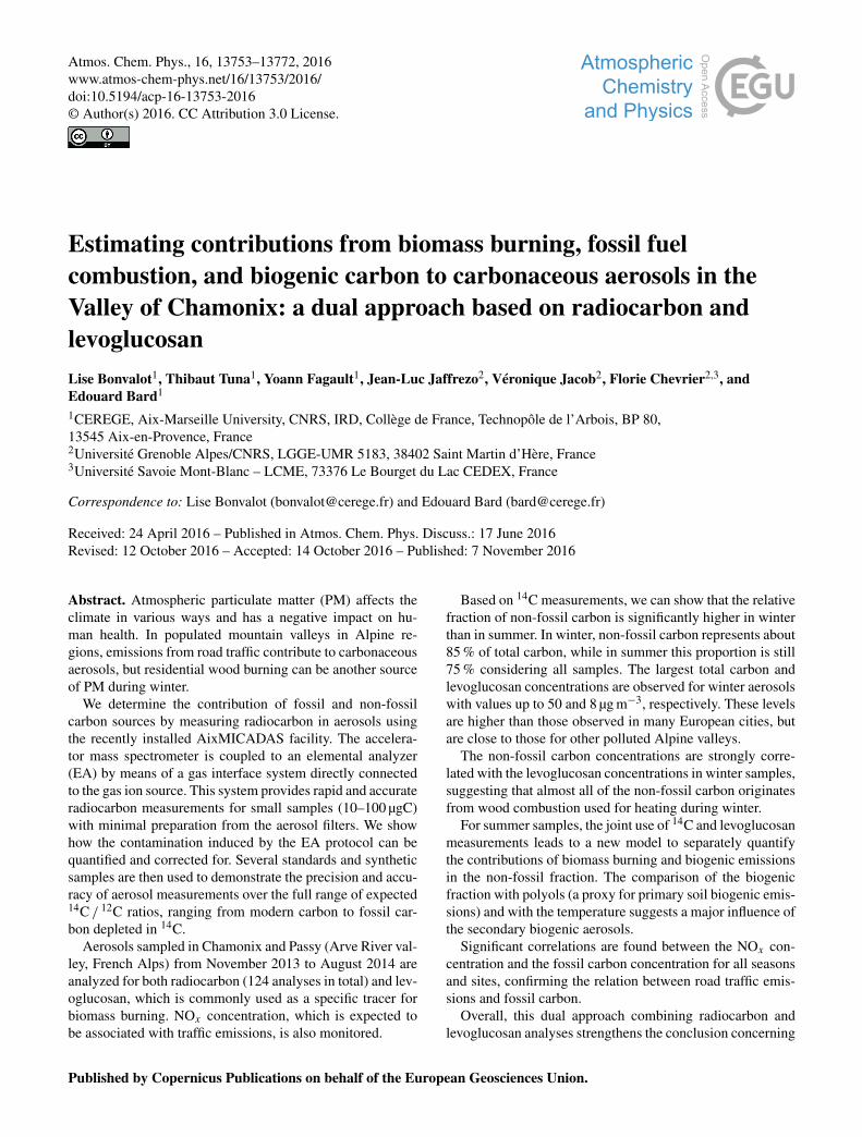
were measured and a nonlinear weighted least squaresmethod (weights corresponding to the measured uncertain-ties on F 14CM values) was applied to determine F 14CCand MC. The results of the contamination model for theblank and the standard are represented in Fig. 1a; the esti-mated parameters from the fit are F 14CC= 0.73± 0.11 andMC= 1.45± 0.26 µgC (95 % confidence interval). Figure 1band c depicts the same dataset corrected for the contamina-tion parameters. It can be observed that F 14CS values for PA

-0.25

-0.20

-0.15

-0.10

-0.05

0.00

0.05

0.10

0.15

0.20

0 20 40 60 80 100 120

14C

/12C

rat

io [

F14C

]

Carbon mass (MS)[µg]

1.20

1.30

1.40

1.50

1.60

1.70

1.80

0 20 40 60 80 100 120

14C

/12C

rat

io [

F14C

]

Carbon mass (MS) [µg]

(b)

(c)

1.00

1.10

1.20

1.30

1.40

0.00

0.10

0.20

0.30

0.40

0 20 40 60 80 100 120

14C

/1

2C O

xA2

[F1

4C]

14C

/12C

PA

[F1

4C

]

Measured carbon mass (MM) [µg]

(a)(a)

Figure 1. Measurements and corrections for blank (phthalic acid,PA) and standard (oxalic acid 2, OxA2) samples. (a) Blue dotsrepresent the measured 14C / 12C ratio for sample blanks and redsquares stand for standard measurements. Solid lines and dashedlines represent the least square optimization with its 95 % confi-dence interval. MM is the measured carbon mass. (b) Blue dots arethe corrected blank measurements. MS is the sample carbon mass(i.e., the measured carbon mass corrected for the contaminant car-bon mass). (c) Red squares are the corrected standard measurementsand the line at 1.3406 stands for the certified value of OxA2. MS isthe sample carbon mass (i.e., the measured carbon mass correctedfor the contaminant carbon mass). The results shown in (b) (blank)and (c) (standard) illustrate the quality of the correction.

and OxA2 are in agreement with the expected values, con-firming the constant contamination assumption. Contamina-tion studies were also carried out without filter punches (theblank and standard are laid in solid forms in the silver boats),leading to similar contamination parameters. It may thus bededuced that the boats are the primary source of contamina-tion.



2.1.3 Standard and synthetic aerosol samples

In order to mimic aerosol samples, two NIST standards wereused as end-members and were mixed together to simulatedifferent 14C / 12C ratios: SRM (Standard Reference Mate-rial) 2975 Forklift Diesel Soot (78 % carbon) and SRM 1515Apple Leaves (45 % carbon). The first standard typifies fossilfuel combustion products while the second provides an ana-log of natural biopolymers generally found in PM (Currieand Kessler, 2005). 14C / 12C ratios were determined by per-forming precise measurements on large samples, of roughly1 mgC, that were graphitized with the AGE-3 system (Au-tomated Graphitization Equipment, described in Wacker etal., 2010) and analyzed with AixMICADAS using its hy-brid ion source in the conventional mode. As expected, SRM2975 exhibits a very low 14C / 12C ratio (F 14C= 0.0013 withSD= 0.0002, N = 5, and σer= 0.0001, blank subtracted)whereas SRM 1515 has the 14C / 12C ratio of the atmosphereat the time of its photosynthesis in 1985 (F 14C= 1.1862 withSD= 0.0017, N = 5, and σer= 0.0007).

Mixtures of the two SRM standards were prepared to ob-tain different 14C / 12C ratios. To ensure homogeneity, thestandards were mixed with an agate mortar and pestle. Therelative proportion of modern carbon can be defined as fol-lows in Eq. (5):

Xmodern carbon =mCSRM1515

mCSRM1515+mCSRM2975

=0.45×mSRM1515

0.45×mSRM1515+ 0.78×mSRM2975. (5)

Expected F 14C values were calculated by using the massof each SRM and their measured F 14C as end-members.The uncertainties were calculated by propagating differentsources of errors: the weighing uncertainty on the massof each standard and the analytical uncertainties of the14C / 12C ratio of the pure standards. All mixed sampleswere graphitized with the AGE-3 system and measured withAixMICADAS (three measurements for each mixture). Thesmall scatter of the results listed in Table 1 confirms that mix-tures were well homogenized and that 14C / 12C ratio deter-minations are reproducible. In addition, the good agreementbetween theoretical and measured values confirms that thesemixtures can be used to simulate small aerosol samples.

Following this initial step, the SRM mixtures were loadedonto quartz filters. In order to simulate real aerosol samples,each powder mixture was suspended in ultrapure water. Dif-ferent volumes of these suspensions (about 80 µgC mL−1)

were then deposited onto quartz filters that had been bakedpreviously at 500 ◦C for 2 h. A vacuum filtration system(Millipore) was used to eliminate most of the water and todistribute carbonaceous particles evenly over the filter sur-face. Loaded filters were dried overnight in a laminar air-flow hood and then subsampled with a puncher (d = 11 mm,S= 0.95 cm2) before being loaded into silver boats. Each

0.0

0.2

0.4

0.6

0.8

1.0

1.2

1.4

0.0 0.2 0.4 0.6 0.8 1.0 1.2 1.4

F14C

gase

ous m

easu

rem

ents

Theoretical F14C

y = ax + ba = 0.992 ± 0.042b = -0.013 ± 0.042

Pearson's r = 0.998

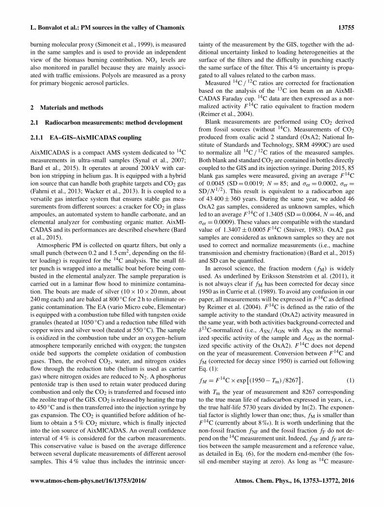
Figure 2. F 14C values of synthetic and standard (test) aerosol sam-ples measured with the gas source compared with theoretical values.These test aerosols are made of two Standard Reference Materials(SRM 2975 and SRM 1515). The compositions of the different mix-tures are listed in Table 1 with the corresponding theoretical andmeasured F 14C. The coefficients of the linear regression have beencalculated by taking into account error bars (2 SD) on both axesand are given with their 95 % confidence interval. The linear rela-tion confirms the accuracy of aerosol measurements with the gasion source over the full range of expected 14C activities.

standard mixture was measured at least four times with dif-ferent carbon masses, corresponding to different loadings onindependent filters. Mean results shown in Fig. 2 confirm theaccuracy of aerosol measurements with the gas ion sourceover the full range of expected 14C activities (F 14C between0.001 and 1.2).

To further test the precision and accuracy of the developedaerosol analytical procedures, we also analyzed two stan-dards prepared from atmospheric particle matter (Table 2).

We acquired NIST SRM 1649b, prepared from the samebulk material as the original SRM 1649 and SRM 1649a(which are no longer available) but sieved to a smaller par-ticle size fraction (63 µm). The original bulk material, SRM1649 was prepared at NIST from PM collected in 1976–1977in the Washington, DC, area over a 12-month period and is-sued in 1982 (Wise and Watters, 2007, 2009).

High-precision measurements were performed to deter-mine the 14C / 12C ratio of NIST SRM 1649b. Samples wereconverted to graphite with the AGE-3 system. Four solid tar-gets (≈ 1 mgC) were measured. Online gas measurementswere also investigated using quartz filters loaded with NISTSRM 1649b. In short, SRM 1649b was suspended in ultra-pure water (about 80 µgC mL−1) and deposited onto previ-ously baked quartz filters. Loaded filters were then dried inthe clean hood, punched, and wrapped into silver boats, readyfor use with the EA-GIS coupled to AixMICADAS. Thereplicates (N = 7) were obtained with carbon mass rangingfrom 7 to 93 µgC.

Our graphite measurements of large samples are in agree-ment with the values reported in the literature for SRM 1649and SRM 1649a (Currie et al., 1984, 2002; Szidat et al., 2004;



Table 1. Analyses of mixtures of SRM 2975 and SRM 1515 standards in the form of solid graphite targets of large samples (roughly 1 mgC).X modern carbon represents the mass fraction of modern carbon; see Eq. (5). The mass fraction of each SRM can be calculated using theircarbon content (i.e., 45 % for SRM1 515 and 78 % for SRM 2975). “Expected F 14C” is calculated by using the mass of each SRM and itsmeasured F 14C as end-members. Measurements are made with solid target (graphitization, roughly 1 mgC).

X modern Expected F 14C Standard error Measured F 14C (after Standard deviationcarbon [F 14C] graphitization) [F 14C]

0 0.0013 0.0001 0.0013 0.0002 (N = 5)0.2 0.2379 0.0185 0.2297 0.0002 (N = 3)0.51 0.6039 0.0131 0.5896 0.0003 (N = 5)0.8 0.9467 0.0096 0.9411 0.0012 (N = 3)1 1.1862 0.0007 1.1862 0.0017 (N = 5)

Table 2. Analyses of SRM1949b with gaseous and solid (roughly 1 mgC) source. Gaseous measurements are made with punches of loadedquartz filters. Comparison with the literature values for SRM 1649 and SRM 1649a.

GaseoussourceF 14C

SD(N = 7)

SolidsourceF 14C

SD(N = 4)

Literature values F 14C

0.505 0.028 0.532 0.004 Solid measurement SRM 1649a:0.523± 0.018 (N = 5) (Szidat et al., 2004)0.507–0.61, depending on the sample preparation (Currie et al.,2002; Wise and Watters, 2007)0.517/0.572 (simple/double combustion) (Heal et al., 2011)Solid measurement SRM 1649:0.61± 0.04 (Currie et al., 1984)

Wise and Watters, 2007; Heal et al., 2011). The F 14C valuefor the online gas measurements is 0.505, with a SD of 0.028,N = 7, and a σer of 0.010, whereas the determined F 14C forthe solid measurements is 0.532 with a SD of 0.004, N = 4,and a σer of 0.002.

Two suggestions could be proposed to explain the smalldifference between solid and gaseous measurements. Somecolloidal fraction or some water-soluble compounds mayhave been lost during sample preparation. If the soluble andinsoluble fractions are of different origins, associated withdifferent isotopic compositions, this could bias the 14C / 12Cratio of the residual material loaded on the filter. Similarly,the ultrafine fraction (< 0.3 µm) not retained by the filter mayhave a different isotopic carbon composition, leading to thediscrepancy between the solid and gaseous measurements.

Such a problem does not affect our results on mixtures ofSRM 2975 and SRM 1515 standards described previously;indeed, these standards are more prone to be isotopicallyhomogeneous because of their simpler composition, as theyboth originate from one source.

The second reference material is RM 8785, composed ofthe fraction lower than 2.5 µm (i.e., PM2.5) of SRM 1649which has been resuspended in air and deposited onto quartzfilters by NIST and SRI International (Cavanagh and Watters,2005; Klouda et al., 2005). Analyses of three punches givean average F 14C of 0.387 and SD of 0.008. This value is in

agreement which measurements performed by five differentlaboratories (Szidat et al., 2013), even if it is positioned at thehigh end of the values (Fig. 3). Szidat et al. (2013) pointedout that 14C / 12C results for RM 8785 exhibit a larger scat-ter than that measured on other PM samples during the sameintercomparison of laboratories. This was probably causedby heterogeneous loading during production of RM 8785 fil-ters by NIST (concentrations ranging from 92 to 2855 µg onto 8.55 cm2 (Cavanagh and Watters, 2005)) or by secondarydeposition of volatile organic compounds (VOCs) onto thefilters.

An additional source of 14C / 12C scatter may be linkedto the heterogeneity of fine particles (< 2.5 µm) constitutingRM 8785. Indeed, its average F 14C value of approximately0.39 is quite different from the value of approximately 0.5measured for SRM 1649a, which was sieved at 125 µm only,and which is the raw material used to produce RM 8785. Thissuggests the possibility of isotopic heterogeneities betweendifferent particle sizes.

2.2 Samples from the Arve River valley

2.2.1 Sampling sites and procedures

The measurements were performed in the framework of theDECOMBIO (deconvolution combustion biomass) program(Chevrier et al., 2016), which focuses on the source appor-



0.00

0.20

0.40

0.60

0.80

1.00

This study Lab 1 Lab 2 Lab 3 Lab 4 Lab 5

14C

/12C

rat

io [

F14C

]

N=3 N=3 N=6 N=3 N=1 N=5

Figure 3. RM 8785 measurements. Black squares and error barsrepresent values and measurement uncertainties at 2σ , described inSzidat et al. (2013). The black line stands for the average value andthe blue ribbon represents the 2σ confidence interval for Labs 1–5.The red square shows the weighted average result obtained for thisstudy (N = 3) and its weighted error (2σ). The large scatter couldbe linked to heterogeneous loading during the production of RM8785 as mentioned by Cavanagh and Watters (2005). The value ob-tained in this study is compatible with the high end of measurementsperformed by the five different laboratories.

tionment of PM10 in the Arve River valley and the evolu-tion of the contribution of biomass burning emissions. Fil-ters analyzed in our study were collected between Novem-ber 2013 and August 2014 in Passy and between Decem-ber 2013 and January 2014 in Chamonix. Both urban sta-tions, maintained by the local Air Monitoring Agency (AirRhône-Alpes) are located in the Arve River valley, in theFrench Alps. The collection sites are presented in Fig. 4.Sampling in the city of Passy (12 000 inhabitants) was per-formed at 583 m a.s.l. (above sea level) whereas samplingin Chamonix (9000 inhabitants) took place at 1035 m a.s.l.For both sampling sites the PM collection occurs about 4 mabove the ground. The Passy sampling station is located ina parking lot, 20 m from the closest house and 90 m froma road. The Chamonix sampling occurred in the city center,close to shops. Temperatures were monitored hourly at bothsites throughout the sampling period. Daily PM10 sampleswere collected on a quartz filter, using a Digitel DA-80 HighVolume Sampler (30 m3 h−1). All filters (quartz filters, PallTissu Quartz, 150 mm Ø) were pre-baked at 500 ◦C for 8 h.They were stored in aluminum foil and sealed in a polyethy-lene sheath before the PM sampling. After collection, filterswere folded, wrapped in aluminum foils, sealed in polyethy-lene bags, and stored at −20 ◦C.

2.2.2 Additional data

Levoglucosan (1,6-anhydro-b-D-glucopyranose) is ananhydro-sugar, emitted by the pyrolysis of cellulose (Si-moneit et al., 1999) and is widely used as a biomass burning

Mont Blanc

Figure 4. Location of the sampling stations in the Arve River val-ley investigated in this study. PM was sampled between Novem-ber 2013 and August 2014 in Passy and between December 2013and January 2014 in Chamonix. Both are urban stations, collectingthe PM10 fraction of atmospheric aerosols.

tracer (Schauer et al., 2001; Jordan et al., 2006a; Caseiroet al., 2009). Here, the levoglucosan is water extracted andthen quantified by high-performance liquid chromatographycoupled with pulsed amperometric detection (Dionex,HPLC DX500 and PAD ED40) (Waked et al., 2014).The concentrations of several polyols (arabitol, mannitol,sorbitol) are also determined by this analysis. Polyols at highconcentration in the atmospheric PM are known to originatefrom emission from fungi from soils (Yttri et al., 2007;Bauer et al., 2008).

TC (total carbon) concentration is also quantified on thesame filters as the determination of the EC (elemental car-bon) and OC (organic carbon) by thermal-optical analysis(TOA) EUSAAR2 (Cavalli et al., 2010) with a Sunset ap-paratus (Birch and Cary, 1996). TC is equal to the sum of ECand OC. PM10 total mass is measured online by TEOMS-FDMS (TEOM 1400ab and FDMS 8500c from Thermo Sci-entific), taking into account the volatile and nonvolatile frac-tions of the PM. NOx (NO+NO2) are also measured online(with the Environnement S.A. AC32M nitrogen oxides ana-lyzer) and are used as proxies for traffic emissions.

2.2.3 Radiocarbon analyses

All samples were analyzed twice to increase the precisionof 14C / 12C and carbon mass data and to check for possi-ble heterogeneity of individual filters. This represents a to-tal of 124 measurements including the sampling blanks (4field blanks for Chamonix and 12 for Passy). Blank sam-pling filters are treated as real samples (in the lab and in thefield) with the exception that no actual sampling is carriedout: they are used to ensure that no significant contaminationoccurs during the different steps of the sampling campaign(e.g., during storage or transport).



Table 3. Results of analysis of Passy samples. PM10 is determined by TEOM-FDMS; days with a PM10 concentration higher than 50 µg m−3

(winter smog) are reported in bold italics (19 February 2014 is sampled with two filters and the sum is greater than 50 µg m−3). Levoglucosanand NOx concentrations: see text. Carbon concentration is determined using the GIS quantification and is expressed with its confidenceinterval. Each radiocarbon value (expressed in F 14C and fM) is based on duplicate measurements: here the weighted mean and its weightederror (2σ , i.e., 95 % confidence interval) are presented. For winter, it is considered that all the non-fossil carbon originates from biomassburning (i.e., fNF,ref = F

14Cbb), whereas all the non-fossil carbon during summer is assumed to originate from biogenic emissions (i.e.,fNF,ref = F

14Cbio). The reference values (fNF,ref) for winter and summer are expressed in F 14C and fM. Fossil and non-fossil fractions(fF and fNF) are determined by the radiocarbon measurements (see Eq. 6).

Date PM10 Carbon ±Carbon Levoglucosan NOx F 14C ±F 14C fM ±fM fNF fF ±fF/

dd/mm/yyyy [µg m−3] mass mass [µg m−3] [µg m−3] fNF[µgC m−3] [µgC m−3]

Winter fNF,ref = 1.10F 14C= 1.09 fM

24/11/2013 31 15.95 0.46 2.37 Nd 0.986 0.010 0.978 0.010 0.90 0.10 0.0203/12/2013 90 48.29 1.39 6.94 Nd 1.002 0.010 0.994 0.010 0.91 0.09 0.0205/12/2013 60 24.56 0.73 3.50 Nd 0.977 0.011 0.970 0.011 0.89 0.11 0.0206/12/2013 69 37.69 1.10 5.14 Nd 1.015 0.011 1.007 0.010 0.92 0.08 0.0208/12/2013 75 38.58 1.12 6.03 Nd 1.047 0.011 1.039 0.011 0.95 0.05 0.0209/12/2013 93 45.87 1.33 6.26 Nd 0.969 0.010 0.962 0.010 0.88 0.12 0.0212/12/2013 133 53.81 1.55 7.66 177 0.987 0.010 0.979 0.010 0.90 0.10 0.0213/12/2013 133 57.14 1.65 8.48 170 0.985 0.010 0.977 0.010 0.90 0.10 0.0215/12/2013 86 34.46 1.01 5.81 68 1.067 0.011 1.059 0.011 0.97 0.03 0.0216/12/2013 108 42.04 1.22 6.29 145 0.964 0.010 0.956 0.010 0.88 0.12 0.0218/12/2013 82 28.78 0.85 4.60 120 0.926 0.010 0.919 0.010 0.84 0.16 0.0220/12/2013 60 25.20 0.74 4.20 81 1.003 0.011 0.995 0.010 0.91 0.09 0.0201/01/2014 25 7.81 0.23 1.15 25 0.978 0.011 0.971 0.010 0.89 0.11 0.0222/01/2014 41 17.35 0.50 2.63 57 0.957 0.011 0.949 0.010 0.87 0.13 0.0212/02/2014 21 7.80 0.23 0.97 34 0.924 0.010 0.917 0.010 0.84 0.16 0.0213/02/2014 18 6.45 0.20 0.83 23 0.980 0.012 0.972 0.011 0.89 0.11 0.0215/02/2014 13 3.76 0.12 0.47 13 0.875 0.013 0.868 0.013 0.80 0.20 0.0216/02/2014 43 16.48 0.48 2.61 32 1.026 0.011 1.018 0.011 0.93 0.07 0.0219/02/2014 38 17.06 0.49 2.69 Nd 0.976 0.011 0.968 0.011 0.89 0.11 0.0219/02/2014 37 17.39 0.50 2.65 Nd 0.924 0.011 0.917 0.011 0.84 0.16 0.0221/02/2014 29 12.06 0.35 1.71 35 1.046 0.011 1.038 0.011 0.95 0.05 0.0222/02/2014 22 7.08 0.21 0.93 24 1.011 0.011 1.003 0.011 0.92 0.08 0.0224/02/2014 38 16.17 0.39 2.09 46 0.878 0.008 0.871 0.008 0.80 0.20 0.0225/02/2014 37 9.81 0.29 1.30 40 0.921 0.011 0.914 0.011 0.84 0.16 0.0227/02/2014 33 12.37 0.36 1.66 46 0.956 0.011 0.949 0.011 0.87 0.13 0.0228/02/2014 20 8.81 0.26 1.31 21 1.004 0.011 0.996 0.011 0.91 0.09 0.0202/03/2014 20 7.25 0.22 1.12 15 1.033 0.011 1.025 0.011 0.94 0.06 0.02

Summer fNF,ref = 1.04 F 14C= 1.03 fM

28/07/2014 15 3.45 0.11 0.03 14 0.714 0.012 0.708 0.012 0.69 0.31 0.0130/07/2014 12 2.81 0.10 0.03 17 0.625 0.015 0.620 0.014 0.60 0.40 0.0231/07/2014 13 3.33 0.11 0.03 11 0.686 0.013 0.680 0.013 0.66 0.34 0.0102/08/2014 17 3.13 0.11 0.03 10 0.815 0.014 0.809 0.014 0.78 0.22 0.0203/08/2014 13 2.81 0.10 0.04 6 0.879 0.016 0.872 0.016 0.85 0.15 0.0205/08/2014 16 3.66 0.12 0.03 11 0.815 0.013 0.809 0.013 0.78 0.22 0.0106/08/2014 21 4.74 0.15 0.04 15 0.771 0.011 0.765 0.011 0.74 0.26 0.0108/08/2014 10 3.17 0.11 0.02 14 0.717 0.013 0.711 0.013 0.69 0.31 0.0109/08/2014 11 3.12 0.10 0.06 11 0.823 0.014 0.816 0.014 0.79 0.21 0.0211/08/2014 13 2.50 0.09 0.06 13 0.771 0.017 0.764 0.017 0.74 0.26 0.0212/08/2014 13 2.73 0.10 0.05 10 0.829 0.016 0.822 0.016 0.80 0.20 0.0214/08/2014 8 1.97 0.08 0.04 9 0.794 0.021 0.788 0.020 0.76 0.24 0.0215/08/2014 7 2.32 0.09 0.13 9 0.890 0.020 0.883 0.020 0.86 0.14 0.0217/08/2014 9 2.39 0.09 0.04 7 0.824 0.018 0.817 0.018 0.79 0.21 0.02



Table 4. Results of analysis of Chamonix samples. PM10 is determined by TEOM-FDMS; days with a PM10 concentration higher than50 µg m−3 (winter smog) are reported in bold italic. Levoglucosan and NOx concentrations: see text. Carbon concentration is determinedusing the GIS quantification and is expressed with its confidence interval. Each radiocarbon value (expressed in F 14C and fM) is basedon duplicate measurements: here the weighted mean and its weighted error (2σ i.e., 95 % confidence interval) are presented. Fossil andnon-fossil fractions (fF and fNF) are determined by the radiocarbon measurements (see Eq. 6).

Date PM10 Carbon ±Carbon Levoglucosan NOx F 14C ±F 14C fM ±fM fNF fF ±fF/

dd/mm/yyyy [µg m−3] mass mass [µg m−3] [µg m−3] fNF[µgC m−3] [µgC m−3]

05/12/2013 44 19.75 0.57 2.66 174 0.900 0.011 0.893 0.011 0.82 0.18 0.0208/12/2013 44 24.80 0.73 3.83 129 1.017 0.012 1.009 0.012 0.92 0.08 0.0211/12/2013 63 29.52 0.87 3.87 250 0.872 0.010 0.865 0.010 0.79 0.21 0.0214/12/2013 40 20.97 0.60 3.23 133 0.968 0.011 0.961 0.011 0.88 0.12 0.0217/12/2013 53 29.97 0.88 3.45 263 0.865 0.011 0.858 0.011 0.79 0.21 0.0220/12/2013 18 7.08 0.21 0.87 74 0.841 0.011 0.834 0.011 0.76 0.24 0.0223/12/2013 39 20.09 0.60 3.02 170 0.914 0.011 0.907 0.011 0.83 0.17 0.0226/12/2013 14 5.73 0.18 0.79 57 0.918 0.012 0.911 0.011 0.83 0.17 0.0229/12/2013 18 8.36 0.25 1.17 67 0.943 0.013 0.935 0.013 0.86 0.14 0.0201/01/2014 61 26.29 0.77 4.21 154 1.018 0.012 1.010 0.012 0.93 0.07 0.0204/01/2014 17 8.48 0.25 1.23 82 0.942 0.011 0.934 0.011 0.86 0.14 0.0207/01/2014 36 19.83 0.57 2.86 161 0.897 0.011 0.890 0.011 0.82 0.18 0.02

Punch surface required for radiocarbon analysis (i.e.,punch of 1 or 0.4 cm2, depending on the carbon loading ofthe filter) was determined using the total carbon concentra-tion previously determined by the EC /OC thermal-opticalanalysis at LGGE (Grenoble). In this study, the carbon quan-tity is also determined by the GIS before CO2 injection intothe ion source.

The mean carbon mass of the sampling blank filters deter-mined by the GIS system is 1.75 µgC (SD= 1.22 µgC, N =16). This contamination level agrees with the independentblank assessment described in Sect. 2.1.2. For real aerosolsamples, the carbon mass and 14C / 12C ratios are thus cor-rected in the same way as described previously.

The carbon content data measured by TOA in the LGGE(Grenoble) and by the GIS in the CEREGE (Aix-en-Provence) are compared in Fig. 5, exhibiting a very stronglinear correlation for both sites (treated together). The slopeis close to 1, with a very small intercept, suggesting there isno major difference between measurements obtained on dif-ferent punch subsamples. This also demonstrates that sam-pling filters are loaded relatively homogenously.

3 Results and discussion

3.1 Composition of PM10

For both sites, summer samples exhibit daily average PM10concentrations up to 21 µg m−3 while winter PM10 concen-trations range from 13 to 133 µg m−3. Above the public infor-mation threshold, 12 days in Passy and 3 days in Chamonixexceed 50 µg m−3 and correspond to winter smog episodes(see Tables 3 and 4). On average, winter samples are com-posed of about 45 % carbon (for both Passy and Chamonix),

0

10

20

30

40

50

60

70

0 10 20 30 40 50 60 70

Car

bo

n c

on

cen

trat

ion

LG

GE

[µgC

m-3

]

Carbon concentration CEREGE (GIS) [µgC m-3]

y = ax + ba = 1.009 ± 0.022b = 0.114 ± 0.112

Pearson's r = 0.998

Figure 5. Total carbon concentration measurements. Comparisonbetween TOA (LGGE in Grenoble) and GIS (CEREGE in Aix-en-Provence) measurements. The grey squares stand for the Chamonixsamples and the black squares stand for the Passy samples. Theregression parameters, given with their 95 % confidence intervals,have been calculated by taking into account error bars on both axesand exhibit a very good correlation between the two carbon concen-trations; the two sets of measurements can be considered as equiva-lent.

while summer samples in Passy comprise 25 % carbon only.The carbon concentration in Passy is very high during thewinter season (average of 23 µgC m−3), particularly duringDecember with a mean concentration of 40 µgC m−3. It ismuch lower during July and August at about 3 µgC m−3. Themean carbon concentration in Chamonix for December andJanuary is about 18 µgC m−3. Therefore, the December av-erage carbon load in Passy is about twice that in Chamonix.Passy is a populated area, located in the lower part of theArve River valley, with a valley constriction (steep slopes andreduced sun exposure) limiting atmospheric mixing in win-



ter. High emissions and a strong temperature inversion layerpersisting for several consecutive days lead to very high par-ticle concentrations when compared to those in Chamonix.

These winter carbon concentrations are an order of magni-tude higher than those determined in Gothenburg (Sweden)during February and March 2005 (3 µgC m−3) (Szidat et al.,2009) or in Hachioji (Japan) during the 2003 and 2004 winterseasons (less than 3 µgC m−3) (Uchida et al., 2010). Com-parable concentrations were observed in Switzerland (Szidatet al., 2007) in Roveredo (about 16 µgC m−3, January 2005)and Moleno (about 24 µgC m−3, February 2005), places thatare also typical Alpine valley sites similar to Passy and Cha-monix.

The summer mean level of levoglucosan in Passy is closeto 0.03 µg m−3, which is comparable to summer backgroundconcentrations determined by Puxbaum et al. (2007) for sixbackground stations located on an east–west line from Hun-gary to the Azores. At our sites, winter levels are about 100times greater than summer ones: in Chamonix, the averageconcentration is about 2.6 µg m−3, while in Passy it is about3.4 µg m−3 (up to 8.5 µg m−3). These levels are similar tothose found in Launceston (Australia) during winter 2003(Jordan et al., 2006a) but are generally higher than winter lev-els measured in various European cities (Herich et al., 2014).

Recent studies report that levoglucosan can be partially de-graded by photo-oxidation (Hennigan et al., 2010; Kessler etal., 2010) for summer conditions, suggesting that this proxyis not as stable as previously thought. However, as wintertemperatures are low (on average between 0 and −2.5 ◦C)and photo-oxidation is reduced by meteorological condi-tions (reduced daylight period, strong presence of smog andclouds) during this season, the levoglucosan level is expectedto be particularly stable during winter. In addition, in ourstudy sampling was carried out close to the emission sources,limiting the exposure time and thus any possible degradation,even during summer.

Levoglucosan emission rate depends on various factors,such as the combustion type and conditions (Engling et al.,2006; Schmidl et al., 2008; Lee et al., 2010). Wood type(softwoods and hardwoods) also has an influence on theemission factor of levoglucosan: as ambient measurementsgenerally represent a mixture of different fuels and combus-tion conditions, the relation between levoglucosan and PMemissions can vary.

3.2 14C-based source apportionment

Carbon in atmospheric aerosols can originate from both fos-sil and contemporary sources. Carbon in particles from fossilfuel emissions is characterized by F 14C= 0, due to the ra-dioactive decay (half-life of 5730 years), whereas F 14C≈ 1for carbon in particles coming from contemporary sources.In addition, the atmospheric thermonuclear bomb tests ofthe late 1950s and early 1960s increased the 14C contentof the atmosphere, leading to F 14C contemporary values

greater than 1. In the Northern Hemisphere, the bomb spikereached F 14C values on the order of 1.8 in the early 1960sand has decayed asymptotically since that time (Levin et al.,2010, 2013; Hua et al., 2013). From these studies, the at-mospheric value for the year 2013–2014 can be estimatedat F 14Catmo = 1.04. Hence, biogenic emissions from theseyears will present the same value (F 14Cbio = 1.04).

3.2.1 Apportionment of the carbon pool with a simplehypothesis

In a first and preliminary approximation, we assume that thecarbonaceous fraction is composed of both a fossil fraction,without 14C and so linked to fossil fuels, and an isotopicallyhomogenous non-fossil fraction. To determine this non-fossilfraction (fNF), the measured F 14C has to be normalized bya non-fossil reference value (fNF,ref, expressed in F 14C) asdescribed by Eq. (6).

fNF =F 14CfNF,ref

(6)

The high levels of levoglucosan obtained during winter il-lustrate the significance of biomass burning at both sitesduring the cold season while summer values suggest thatvery little biomass burning is recorded for the warm sea-son. Biomass burning is mainly based on wood that grewover the past decades. This means that this carbon fractionintegrates an average F 14C that is slightly higher than thatof the atmosphere at the time of sampling. As per Szidat etal. (2006) and Lewis et al. (2004), we assume that woodused for biomass burning has an average F 14Cbb = 1.10(fM,bb = 1.09), which can be retrieved from the atmospheric14C record combined with a tree growth model.

For the summer season, it is considered that all non-fossilcarbon originates from organic compounds naturally releasedby living plants (Guenther et al., 1995). No wildfire wasrecorded during the sampling period and the influence ofthe charcoal from barbecue cooking is neglected; levels ofcholesterol, generally emitted by meat charbroiling (Schaueret al., 1999) remain very low, indicating that this cookingtechnique is not important here. Therefore, only the biogenicsource of aerosols is considered, whose F 14C value shouldbe close to the atmospheric value at the time of sampling(F 14Cbio = 1.04).

Hence, for this first estimation of the non-fossil and fossilfractions, fNF,ref is estimated to be equal to 1.10F 14C for thewinter samples and to 1.04F 14C for the summer ones.

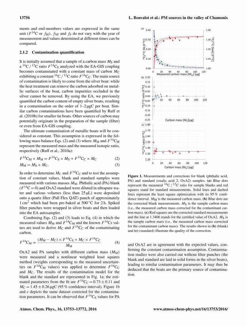
The calculated non-fossil fraction (fNF) for the wintersamples (Fig. 6) exhibits high values, with mean valuesequal to 0.89 and 0.84 for Passy and Chamonix, respec-tively. Lower values observed at Passy in summer (meanfNF = 0.75) indicate that the fossil component is more im-portant in relative term to the total carbon content of aerosols,but that an important non-fossil fraction is still largely domi-nant.



The concentrations of non-fossil carbon (TCNF) and fossilcarbon (TCF) can be calculated by multiplying the total car-bon concentration (TC) by the non-fossil fraction (fNF) andthe fossil fraction (fF), respectively.

While the mean TC is about 13 times larger in winterthan summer, the fossil carbon concentration TCF exhibitsa smaller variation between seasons, as expected from simi-lar traffic over the year. Nonetheless, the TCF winter concen-tration is still about 3 times the summer one, which may berelated to the reduced atmospheric dynamics during winter,leading to trapping of particles by the inversion layers.

Schmidl et al. (2008) demonstrated that combustion of fivebiomass fuel types (spruce, larch, beech, oak, and briquettes)at similar burning conditions leads to a wide range of to-tal carbon to levoglucosan ratios, from 4.3 to 17.2. In theirstudy, the TC only originates from wood combustion and canthus be considered as completely non-fossil TC. The meanTCNF / levoglucosan ratios equal 6.2 (SD= 0.4, N = 28) forPassy and 6.0 (SD= 0.3, N = 13) for Chamonix. These ra-tios are within the range, but do not correspond to any par-ticular wood type, as presented by Schmidl et al. (2008).However, the TCNF / levoglucosan ratios for Chamonix andPassy are in good agreement with those obtained by Zotteret al. (2014) for several Swiss stations in the southern Alpswith ratios close to 6.2± 2.0, with the exception of Chiassostation (TCNF / levo ratio about 9.1± 2.6).

The TCNF values are plotted against levoglucosan inFig. 7, and show a linear relation with high correlation coeffi-cients for Chamonix (Pearson’s r = 0.989) and Passy (Pear-son’s r = 0.995) samples. Moreover, the intercepts are notstatistically different from zero, showing that virtually allTCNF during winter originates from the burning of biomass,and more specifically, from wood combustion used for heat-ing.

One interesting point with these excellent correlationsis their stability, considering the large array of samples,which may include samples with various aging histories andthus variable amounts of secondary aerosols produced fromVOCs emitted during biomass combustion. Nevertheless, thecorrelations are established between a primary tracer (lev-oglucosan) and a total carbon quantity, which includes bothprimary and secondary carbonaceous aerosols. Therefore,the excellent correlation implies either that the primary par-ticles are dominant (in general for the total emission or be-cause the secondary formation is slow in our conditions) orthat the fraction of secondary particles is constant in relativeterms (i.e., the correlation would remain even if secondaryparticles were dominant).

As a purely hypothetical case, let us assume that sec-ondary organic aerosols (SOA) vary between 25 and 50 %by OC mass of the primary organic aerosols (POA), accord-ing to VOC conversion kinetics (i.e., 25 % in a recent air and50 % in an older one). The majority of carbonaceous aerosolswould still be composed of primary aerosols, ranging from80 to 67 % of the total carbon, for the two end-members.

0.40

0.50

0.60

0.70

0.80

0.90

1.00

1.10

0

10

20

30

40

50

60

70

24/1

1/20

13

03/1

2/20

13

05/1

2/20

13

06/1

2/20

13

08/1

2/20

13

09/1

2/20

13

12/1

2/20

13

13/1

2/20

13

15/1

2/20

13

16/1

2/20

13

18/1

2/20

13

20/1

2/20

13

01/0

1/20

14

22/0

1/20

14

12/0

2/20

14

13/0

2/20

14

15/0

2/20

14

16/0

2/20

14

19/0

2/20

14

19/0

2/20

14

21/0

2/20

14

22/0

2/20

14

24/0

2/20

14

25/0

2/20

14

27/0

2/20

14

28/0

2/20

14

02/0

3/20

14

28/0

7/20

14

30/0

7/20

14

31/0

7/20

14

02/0

8/20

14

03/0

8/20

14

05/0

8/20

14

06/0

8/20

14

08/0

8/20

14

09/0

8/20

14

11/0

8/20

14

12/0

8/20

14

14/0

8/20

14

15/0

8/20

14

17/0

8/20

14

fNF

TC [

µgC

m-3

]

TC fNF (pbio = 1) fNF (pbio = 0.4) fNF (pbio = 0.2) fNF (pbio = 0)

SummerWinter

0.40

0.50

0.60

0.70

0.80

0.90

1.00

1.10

0

5

10

15

20

25

30

35

fNF

TC [

µgC

m-3

]

TC fNF (pbio = 1) fNF (pbio = 0.4) fNF (pbio = 0.2) fNF (pbio = 0)

(a) Passy

(b) Chamonix

Figure 6. Results for (a) Passy and (b) Chamonix. Grey bars repre-sent carbon concentration. Days with a PM10 concentration higherthan 50 µg m−3 are marked with a yellow star. Green diamondsstand for the only biogenic fNFref, pink squares are for fNFref witha 40 % biogenic fraction, purple triangles denote fNFref with a 20 %biogenic fraction, and red dots stand for fNFref with a 0 % biogenicfraction. In all cases, the non-fossil fraction remains at very highlevels during the winter season, validating the importance of thenon-fossil source. A maximum variation of 6 % is observed in thedifferent fNF estimations.

However, because the dynamic range of total emissions isvery large, this variability due to aerosol aging is difficult todetect on the TCNF vs. levoglucosan diagram (Fig. 7).

Keeping the same educated guess would imply that for aparticular levoglucosan concentration value, one could ob-serve a 20 % range of TCNF (i.e., 150/125= 1.2). To illus-trate this in Fig. 7, we show two extreme cases assumingonly young air (i.e., SOA= 25 % of POA) or only older air(i.e., SOA= 50 % of POA). For the same value of levoglu-cosan, the TCNF ratio between the two extremes should be1.2, which can be approximated by decreasing or increas-ing the observed slope by about 10 % (dotted lines in Fig. 7)around the observed correlation assumed to be centered be-tween the two end-members. Even if the observed correlationin Fig. 7 is strong, it is clear that its scatter is not completelynegligible, but is within the variation between the two hypo-



Figure 7. Comparison of TCNF, based on 14C / 12C ratio measure-ments, with levoglucosan. TCNF corresponds to the carbon concen-tration multiplied by the fNF. For the winter samples, fNF is de-termined for pbio = 0 and for summer samples, pbio = 1. It has tobe underlined that a variation in pbio does not affect the signifi-cance of the relationship between levoglucosan and TCNF (see Ta-ble 5). Purple squares indicate Chamonix winter samples, red dotsPassy winter samples, and blue dots denote Passy summer samples.Winter samples display very strong correlations between TCNF andlevoglucosan with close to zero intercepts, suggesting that virtuallyall of the TCNF originates from biomass burning. The fit parame-ters have been calculated by taking into account both error bars onthe x and y axes and are given with their 95 % confidence interval.Black dotted lines stand for two extreme cases assuming only youngair (i.e., SOA= 25 % of POA) or only older air (i.e., SOA= 50 %of POA); see Sect. 3.2.1 for further information. No correlation isfound for the summer samples, implying the summer TCNF origi-nates from other non-fossil sources.

thetical extremes (see for examples the TCNF values corre-sponding to about 6 µg m−3 of levoglucosan). These observa-tions and speculations would certainly justify specific studieson secondary aerosol formation processes in the atmosphericconditions of the Arve River valley.

During summer, domestic heating emissions are presumedto be weak, as confirmed by really low levoglucosan con-centrations. Levoglucosan and TCNF concentrations show nocorrelation for summer samples (represented by blue dots inFig. 7). As mentioned above, TCNF still represents on aver-age 75 % of the total carbon in summer. It has already beendemonstrated that the modern sources of carbon are domi-nant over the fossil fuel ones in atmospheric PM of manysites, even in a large city like Marseille, France (El Haddadet al., 2011). This is also the case in these more rural envi-ronments. These TCNF levels are about 4 times higher thanexpected by the regression model determined for the win-ter samples if they were due to biomass burning. These re-sults indicate that the main non-fossil sources differ betweenseasons. For the winter season, TCNF is directly related tobiomass burning, whereas during summer these sources aremost probably biogenic emissions.

-1

0

1

2

3

4

5

6

7

0 50 100 150 200 250 300

TCF

[µgC

m-3

]

NOX [µg m-3]

Passy wintery = ax + b

a = 0.036 ± 0.003b = 0.062 ± 0.086

Pearson's r = 0.950

Passy summery = ax + b

a = 0.103 ± 0.012b = -0.366 ± 0.124Pearson's r = 0.822

Chamonix wintery = ax + b

a = 0.024 ± 0.002b = -0.467 ± 0.213Pearson's r = 0.959

Figure 8. Comparison of TCF, based on 14C / 12C ratio measure-ments, with NOx . TCF corresponds to the carbon concentrationmultiplied by fF. For the winter samples, fF is determined forpbio = 0 and for summer samples pbio = 1. It has to be under-lined that a variation in pbio does not affect the significance of therelationship between levoglucosan and TCNF (see Table 5). Pur-ple squares denote Chamonix winter samples, red dots denote Passywinter samples, and blue dots designate Passy summer samples.Each dataset exhibits a good correlation between NOx and TCFconcentrations. The fit parameters have been calculated by takinginto account both error bars on the x and y axes and are given withtheir 95 % confidence interval. A higher slope value is obtained forthe summer datasets than for the winter ones, which suggests eitherdifferent fossil carbon sources or NOx degradation rate dependingon the season.

To attribute the fossil fraction of the carbonaceous parti-cles, the concentrations of fossil carbon (TCF) are plottedagainst NOx concentration (Fig. 8), which is considered asa vehicle emission proxy. Linear correlations are highly sta-tistically significant for all three different datasets. All originintercepts are equivalent or close to zero. For winter datasets,the slope obtained for the French datasets are roughly equiv-alent to those given by Zotter et al. (2014) for the ECF vs.NOx correlations in many Swiss sites (no correlations wereobserved with OCF in this last study). However, in our study,the slopes for Passy and Chamonix are clearly different, withthat in Passy being 50 % higher. The reason for such a differ-ence is currently unknown, but may be related to the vehiclefleet influencing the two sites: while the site in Chamonix isan urban traffic site with only passenger vehicles, the site inPassy is an urban background site 1 km away from the high-way to Italy, which supports a large amount of internationaltruck traffic. Also, the impact of some industrial emissions inPassy remains to be investigated.

The slope obtained for the summer samples (only in Passy)is larger than that obtained for winter, which may suggestdifferent vehicular emissions in summer than in winter or anextensive degradation of NOx during summer. Another hy-pothesis is that secondary formation of OC from vehicular



gaseous emissions may well be greater in summer than inwinter.

3.2.2 Apportionment with biogenic fraction variations

The calculations above only constitute a first approximationthat takes into account a single non-fossil source to definefNF,ref. So far, we considered the non-fossil source to bepurely biogenic during summer and to originate exclusivelyfrom biomass burning only during winter. However, the non-fossil carbon is made up of these two different fractions thatdiffer slightly in their 14C / 12C ratios, and both have to beacknowledged in the definition of fNF,ref.

Zhang et al. (2012) assumed a biogenic fraction (pbio)

constant throughout the year, implying that its origin doesnot vary with the season. More recently, Zotter et al. (2014)applied a variability with the seasons: the biogenic fractionis set at 0.4 during summer and 0.2 during winter since nolarge contributions from biogenic sources are expected dur-ing the cold season. With these two assumptions, the max-imum F 14C value in the absence of a fossil component isgiven by the following mass balance equation Eq. (7) (Szidatet al., 2006; Zhang et al., 2012; Zotter et al., 2014):

fNF,ref = pbio×F14Cbio+ (1−pbio)× F

14Cbb, (7)

where F 14Cbio and F 14Cbb correspond to the F 14C valuesof the biogenic (1.04) and the biomass burning components(1.10), respectively. Similarly, pbio corresponds to the bio-genic fraction in the total non-fossil carbon, whereas thebiomass burning fraction is simply (1−pbio). Figure 6 showsthe time series of the fNF values calculated by using both thesimple and sophisticated models for both sites. In all cases,it must be noted that introducing various values of pbio has aminor impact on fNF,ref. Indeed, a decrease of pbio from 1 to0 would change fNF,ref by 6 %. In the same way, the regres-sion parameters for the TCNF vs. levoglucosan correlationsare listed in Table 5 for the different values of fNF,ref (i.e.,with pbio = 1, 0.4, 0.2, and 0). It can be seen that the smallvariation of fNF,ref has a negligible impact on the linear re-gression parameters. All approaches confirm the dominanceof the biomass burning component during winter, as illus-trated in Fig. 6.

Table 5 also provides all parameters for the TCF vs. NOxlinear fits. Again, correlation coefficients are significant forall values of pbio (1, 0.4, 0.2, and 0), confirming that intro-ducing the hypotheses for this second model does not lead tochanges in the source partitioning.

3.2.3 Apportionment for summer samples:independent determination of the non-fossilfraction

One inherent problem with the previous model is that it relieson a priori assumptions about the sources of the non-fossilfraction. In addition, it assumes that the biomass burning and

biogenic concentrations (TCbb and TCbio) are proportionalto TCNF, which also implies a linear correlation between thetwo fractions, i.e., TCbb = [(1−pbio)/pbio]×TCbio. Indeed,one could well imagine a variable emission of biomass burn-ing superimposed on a rather constant emission of biogenicparticles, or even a more complex situation as the two sourceshave different and rather independent origins.

In Sect. 3.2.1, the nearly exclusive contribution of biomassburning to the non-fossil fraction during winter has beendemonstrated by the strong linear correlation between lev-oglucosan and TCNF (Fig. 7 and Table 5) and by interceptsnearly equal to zero (i.e., TCNF ≈ TCbb during winter). Forsummer samples, the insert in Fig. 7 shows that the TCbb ex-pected by the linear models is lower than the measured TCNF,suggesting another source of non-fossil carbon.

As an alternative model, we tentatively propose that thepart of TCNF due to biomass burning (TCbb) in a particularsample could be calculated from its levoglucosan concentra-tion by using its linear correlation to TCNF observed in win-ter (i.e., TCbb= a× [levoglucosan], a being the slope of thelinear relationship shown in Fig. 7).

Total carbon (TC) is composed of both fossil TCF and non-fossil fraction TCNF. The latter can be subdivided into partscorresponding to the considered sources, i.e., biomass burn-ing and biogenic emissions (TCbb and TCbio, respectively).

TC= TCNF+TCF = TCbb+TCbio+TCF (8)

This leads to the following 14C mass balance:

TC×F 14CS = TCbb×F14Cbb+TCbio×F

14Cbio

+TCF×F14CF = TCbb×F

14Cbb

+TCbio×F14Cbio, (9)

with F 14CS as the measured 14C / 12C ratio of the sam-ple, F 14Cbb = 1.10, F 14Cbio = 1.04, and F 14CF = 0 as pre-viously discussed in Sect. 3.2.1. TC is the total carbon ofthe sample [µgC m−3], TCbb is the carbon originating frombiomass burning, TCbio is the carbon from biogenic emis-sions, and finally TCF is the carbon from fossil sources.

It is thus possible to calculate the biogenic fraction and thefossil fraction by combining the 14C mass balance in Eq. (10)and the total carbon mass balance in Eq. (11).

TCbio =F 14CS×TC−TCbb×F

14Cbb

F 14Cbio(10)

TCF = TC−TCbb−TCbio (11)

The results for summer samples are provided in Table 6. Itshould be stressed that this model relies on the hypothesisthat levoglucosan does not suffer from a large differentialdegradation between summer and winter, which may be validto a first order as PM sampling has been carried out close tothe emission sources. The contribution of fossil carbon to TCis estimated to be about 25 %, corresponding to very low fos-sil carbon concentration, i.e., 0.80 µgC m−3. By contrast, the



Table 5. Determination of the linear fit parameters (with their 95 % confidence intervals) for the linear relation between TCNF and levoglu-cosan, and for the linear relation between TCF and NOx . Variation in pbio and in TCNF and TCF does not have a major influence on theregression parameters in the case of TCNF vs. Levoglucosan but does in the case of TCF vs. NOx because of the small amount of TCF.

TCNF vs. Levoglucosan TCF vs. NOx

a ±a b ±b Pearson’s r a ±a b ±b Pearson’s r

Passy summer – – – – – 0.103 0.012 −0.366 0.124 0.822pbio = 1Passy summer – – – – – 0.099 0.014 −0.270 0.145 0.813pbio = 0.4Passy summer – – – – – 0.100 0.014 −0.259 0.145 0.809pbio = 0.2Passy summer – – – – – 0.107 0.013 −0.284 0.132 0.806pbio = 0Passy winter 6.33 0.20 0.38 0.29 0.995 0.024 0.002 −0.040 0.063 0.782pbio = 1Passy winter 6.11 0.20 0.38 0.30 0.995 0.028 0.004 0.127 0.134 0.914pbio = 0.4Passy winter 6.04 0.20 0.37 0.30 0.995 0.031 0.004 0.129 0.133 0.935pbio = 0.2Passy winter 5.98 0.19 0.36 0.28 0.995 0.036 0.003 0.062 0.086 0.950pbio = 0Chamonix winter 6.29 0.35 0.12 0.54 0.989 0.019 0.002 −0.490 0.167 0.885pbio = 1Chamonix winter 6.06 0.35 0.13 0.55 0.989 0.021 0.003 −0.392 0.283 0.938pbio = 0.4Chamonix winter 6.00 0.35 0.13 0.54 0.989 0.023 0.003 −0.407 0.283 0.949pbio = 0.2Chamonix winter 5.94 0.33 0.12 0.51 0.989 0.024 0.002 −0.467 0.213 0.959pbio = 0

results point to a major contribution of about 87 % and upto 93 % of biogenic emissions to the non-fossil fraction (i.e.,pbio is about 0.9).

The biogenic carbon concentrations (TCbio) can be com-pared to the concentrations of polyols as these sugar–alcohols are known to be tracers for primary biogenic aerosolparticles (Yttri et al., 2007). As shown in Fig. 9, there is nosimple relationship between TCbio and polyols for the sum-mer samples, indicating that despite its potential to be a largecontributor to PM10 in some environments (Waked et al.,2014), this source may not be dominant in the modern frac-tion of carbon in summer in the Arve River valley.

TCbio includes both primary and secondary organicaerosols, which result from the oxidation of biogenic volatileorganic carbon compounds (BVOCs). It is known that BVOCemissions generally follow the temperature (Leaitch et al.,2011). Indeed, Fig. 10 shows that TCbio increases withthe mean temperature during the warmest part of the day(from 10:00 to 18:00 UTC+ 01:00 for winter samples andUTC+ 02:00 for summer samples) defining a significant lin-ear correlation (Pearson’s coefficient of 0.65 with a slopeof 0.27± 0.05 and y intercept of −3.41± 1.06). Given thephysiological effect of temperature, it is logical to expect thatemissions are negligible at the low temperature, which can be

0.0

1.0

2.0

3.0

0.00 0.02 0.04 0.06 0.08 0.10 0.12

TCb

io [µ

gC m

-3]

Polyol [µg m-3]

Figure 9. Comparison of TCbio based on levoglucosan and14C / 12C ratio measurements against polyol concentrations. Bluedots stand for the Passy summer samples. No correlation is foundbetween TCbio and polyol concentrations (primary biogenic emis-sions tracers). TCbio could originate from secondary organic carbonfrom the oxidation of biogenic VOC.


L. Bonvalot et al.: PM sources in the valley of Chamonix 13767Ta

ble

6.R

esul

tsof

sum

mer

sam

ples

from

Pass

y.T

Cbb

isca

lcul

ated

from

levo

gluc

osan

conc

entr

atio

n.T

Cbi

oan

dT

CF

com

eou

tfro

mT

Cbb

and

theF

14C

ofth

esa

mpl

e.T

CN

F/

TC

and

TC

F/

TC

are

equi

vale

nttof

NF

andf

Fde

term

ined

dire

ctly

by14

Cm

easu

rem

ents

.The

maj

orpa

rtof

TC

NF

isco

mpo

sed

ofT

Cbi

o.T

heun

cert

aint

ies

repr

esen

tthe

confi

denc

ein

terv

als

(95

%)a

ndar

ede

term

ined

byun

cert

aint

ies

prop

agat

ion.

Dat

eT

Cbb

±T

Cbb

TC

bio

±T

Cbi

oT

CF

±T

CF

TC

NF/

TC

TC

F/

TC

TC

bio/

TC

NF

poly

ol±

poly

oldd

/mm

/yyy

y[µ

gCm−

3 ][µ

gCm−

3 ][µ

gCm−

3 ][µ

gCm−

3 ][µ

gCm−

3 ][µ

gCm−

3 ][n

gm−

3 ][n

gm−

3 ]

28/0

7/20

140.

180.

022.

180.

091.

090.

150.

680.

320.

9264

.56

6.46

30/0

7/20

140.

210.

021.

470.

081.

140.

120.

600.

400.

8879

.88

7.99

31/0

7/20

140.

210.

021.

980.

091.

150.

140.

660.

340.

9074

.04

7.40

02/0

8/20

140.

180.

022.

260.

100.

690.

140.

780.

220.

9280

.91

8.09

03/0

8/20

140.

260.

032.

100.

100.

450.

140.

840.

160.

8980

.23

8.02

05/0

8/20

140.

190.

022.

670.

110.

800.

160.

780.

220.

9365

.20

6.52

06/0

8/20

140.

250.

033.

250.

131.

240.

200.

740.

260.

9355

.61

5.56

08/0

8/20

140.

140.

022.

030.

091.

000.

140.

690.

310.

9385

.26

8.53

09/0

8/20

140.

360.

042.

090.

100.

670.

150.

780.

220.

8576

.51

7.65

11/0

8/20

140.

380.

041.

450.

090.

670.

130.

730.

270.

7962

.80

6.28

12/0

8/20

140.

270.

031.

890.

090.

570.

140.

790.

210.

8794

.51

9.45

14/0

8/20

140.

250.

031.

240.

080.

480.

110.

760.

240.

8350

.09

5.01

15/0

8/20

140.

760.

081.

190.

120.

380.

170.

840.

160.

6145

.14

4.51

17/0

8/20

140.

250.

031.

630.

090.

510.

130.

790.

210.

8738

.93

3.89

0.0

1.0

2.0

3.0

5 10 15 20 25 30

TCb

io[µ

g m

-3]

Temperature [°C]

Passy summery = ax +b

a = 0.27 ± 0.05b = -3.41 ± 1.06

Pearson's r = 0.65

Passy summery = α exp (βx)α = 0.12 ± 0.02β = 0.16 +0.09

-0.06

Pearson's r = 0.72(from natural logarithm

linear fitting)

Figure 10. Comparison of TCbio based on levoglucosan and14C / 12C ratio measurements plotted vs. the average temperatureof the warmest part of the day (10:00 to 18:00 UTC+ 02:00). Bluedots stand for the Passy summer samples. TCbio concentration in-creases with the temperature. Both linear (dashed line) and expo-nential (solid line) relations are represented with their correlationcoefficient. The fit parameters have been calculated by taking intoaccount both error bars on the x and y axes and are given withtheir 95 % confidence interval. The exponential fit is preferred as theTCbio emission cannot be negative. Moreover, emission of BVOCs(precursors of SOA) emission rate is classically described with anexponential law (Leaitch et al., 2011).

approximated by an exponential law given in Eq. (12) as inLeaitch et al. (2011).

TCbio = α× exp(β × T ), (12)

where T is expressed in degrees Celsius, α is a constant,which could be assimilated to a base capacity, and β is anempirical constant. By studying the linear correlation be-tween ln(TCbio) and temperature, it is possible to calculateα = 0.12± 0.02 and β = 0.16 (+0.09/−0.06), with a Pear-son’s coefficient of 0.72. The correlation coefficient is thusslightly higher for the exponential law than for the linearmodel. In any case, the fact that TCbio depends on temper-ature suggests that this fraction is mainly composed of sec-ondary organic aerosol.

4 Conclusions

Quantifying the relative contribution of fossil and non-fossilsources of carbonaceous aerosols is important in order to bet-ter understand the sources of atmospheric particles and to at-tribute them to natural and anthropogenic processes. For ex-ample, both biomass burning for domestic heating and roadtraffic emissions are known to contribute to PM pollution inmany urban areas, notably in the Arve River valley (FrenchAlps), which is the focus of this study.

Radiocarbon (14C) analysis is the best way to distinguishfossil fuel combustion products from other carbon sources



such as biomass burning and biogenic emissions. We showhere that 14C is efficiently measured in aerosol samples withthe AixMICADAS spectrometer by using an elemental ana-lyzer (EA) coupled to its CO2 gas ion source, which can han-dle small samples (10–100 µgC). This direct coupling avoidsthe production of solid graphite targets, which is the usualbottleneck in traditional radiocarbon measurement by accel-erator mass spectrometry. The present work leads to the fol-lowing conclusions:

– Contamination of the measurement procedure is mainlylinked to the silver boats in which the filter samples arewrapped prior to combustion in the EA. This contami-nation has been quantified and shown to be fairly con-stant, which enables rectification of the measurementsof aerosol samples.

– The precision and accuracy of 14C measurements inaerosols are validated over the full range of expectedfossil and non-fossil carbon values by using variousstandards and synthetic mixtures.

– Carbon concentrations of aerosols determined bythermal-optical analysis (LGGE in Grenoble) andGIS quantification (CEREGE in Aix-en-Provence) insamples from Passy and Chamonix are in excellentagreement and indicate large concentrations of up to50 µgC m−3 during winters.

– Mean winter carbon concentrations are higher thanthose reported for several urban sites but are in the rangeof those measured in other Alpine sites.

– Levoglucosan content is used as a biomass burningproxy, indicating very high levels during winter withvalues of up to 8 µg m−3 in Passy, thus higher than thosegenerally observed in several European cities.

– Based on 14C measurements, the fractions of non-fossilcarbon determined in winter (0.89 for Passy and 0.84for Chamonix) are higher than the non-fossil fractionobtained for Passy during summer (0.75). However, thenon-fossil fraction remains dominant during summerwith a fossil contribution of about 25 %, probably fromroad traffic.

– Non-fossil carbon concentration (TCNF) is strongly cor-related with levoglucosan concentration for winter sam-ples (Passy and Chamonix). The linear regression inter-cepts are close to zero suggesting that almost all of thenon-fossil carbon originates from biomass burning andmore specifically from wood combustion used for heat-ing during the winter.

– Fossil carbon concentrations exhibit a strong correlationwith NOx concentrations, suggesting that the source offossil carbon is directly linked to traffic emissions.

– Summer samples exhibit an important relative contri-bution of non-fossil sources (75 %). A dual approachbased on 14C and levoglucosan enables the calculationof a first estimation of the biogenic and biomass burn-ing fractions in the non-fossil carbon. The samples fromPassy allow to test this new model, suggesting that forthis site the biogenic emissions are the most importantcontributor to the non-fossil fraction during summer.

– The lack of correlation between polyols (tracers of bio-genic activity in soil) and the biogenic fraction sug-gests that TCbio could be composed of secondary or-ganic aerosols resulting from the oxidation of biogenicVOC, which is also suggested by the correlation be-tween TCbio and temperature.

Overall, combining radiocarbon and levoglucosan mea-surements strengthens findings concerning the domi-nant contribution of winter biomass burning to aerosolsin the Arve River valley. In addition to first-order agree-ment, both tracers are complementary: levoglucosan en-ables the identification of the source while 14C allowsthe precise quantification of the fossil and non-fossilfractions.

We show that this dual approach may also serve to gofurther in quantifying these additional carbon sources.Combining 14C and levoglucosan measurements allowsreconstruction of other contributions such as biogenicaerosols fluxes. As an example, our new model is ap-plied to summer samples from Passy leading to rea-sonable evaluations of biogenic particle fluxes. Theseaerosols are probably linked to oxidation of volatile or-ganic compounds (VOCs) as suggested by a significantcorrelation of fluxes with temperature.

Following Zhang et al. (2012), ongoing research atCEREGE into 14C measurements of separated ele-mental carbon and organic carbon fractions of aerosolshould provide more precise source apportionment inthe future.

5 Data availability

Detailed data are available as a Supplement.

The Supplement related to this article is available onlineat doi:10.5194/acp-16-13753-2016-supplement.

Acknowledgements. AixMICADAS was acquired and is operatedin the framework of the EQUIPEX project ASTER-CEREGE(PI E. Bard) with additional matching funds from the Collègede France, which also supports the salaries of the authors fromCEREGE. We thank Sönke Szidat for advice on reporting 14C re-sults on aerosols.


http://dx.doi.org/10.5194/acp-16-13753-2016-supplement


Edited by: W. MaenhautReviewed by: three anonymous referees

References

Aymoz, G., Jaffrezo, J. L., Chapuis, D., Cozic, J., and Maenhaut,W.: Seasonal variation of PM10 main constituents in two valleysof the French Alps. I: EC /OC fractions, Atmos. Chem. Phys., 7,661–675, doi:10.5194/acp-7-661-2007, 2007.

Bard, E., Tuna, T., Fagault, Y., Bonvalot, L., Wacker, L.,Fahrni, S., and Synal, H.-A.: AixMICADAS, the accelera-tor mass spectrometer dedicated to 14C recently installed inAix-en-Provence, France, Nucl. Instrum. Meth. B, 361, 80–86,doi:10.1016/j.nimb.2015.01.075, 2015.

Bauer, H., Claeys, M., Vermeylen, R., Schueller, E., Weinke, G.,Berger, A., and Puxbaum, H.: Arabitol and mannitol as tracersfor the quantification of airborne fungal spores, Atmos. Environ.,42, 588–593, doi:10.1016/j.atmosenv.2007.10.013, 2008.

Birch, M. E. and Cary, R. A.: Elemental carbon-basedmethod for monitoring occupational exposures to par-ticulate diesel exhaust, Aerosol Sci. Tech., 25, 221–241,doi:10.1080/02786829608965393, 1996.

Bond, T. C., Doherty, S. J., Fahey, D. W., Forster, P. M., Berntsen,T., DeAngelo, B. J., Flanner, M. G., Ghan, S., Kärcher, B., Koch,D., Kinne, S., Kondo, Y., Quinn, P. K., Sarofim, M. C., Schultz,M. G., Schulz, M., Venkataraman, C., Zhang, H., Zhang, S.,Bellouin, N., Guttikunda, S. K., Hopke, P. K., Jacobson, M.Z., Kaiser, J. W., Klimont, Z., Lohmann, U., Schwarz, J. P.,Shindell, D., Storelvmo, T., Warren, S. G., and Zender, C. S.:Bounding the role of black carbon in the climate system: A sci-entific assessment, J. Geophys. Res.-Atmos., 118, 5380–5552,doi:10.1002/jgrd.50171, 2013.

Caseiro, A., Bauer, H., Schmidl, C., Pio, C. A., and Puxbaum, H.:Wood burning impact on PM10 in three Austrian regions, Atmos.Environ., 43, 2186–2195, doi:10.1016/j.atmosenv.2009.01.012,2009.

Cavalli, F., Viana, M., Yttri, K. E., Genberg, J., and Putaud, J.-P.:Toward a standardised thermal-optical protocol for measuringatmospheric organic and elemental carbon: the EUSAAR proto-col, Atmos. Meas. Tech., 3, 79–89, doi:10.5194/amt-3-79-2010,2010.

Cavanagh, R. R. and Watters, R. L.: Report of investigation Refer-ence Material 8785 air particulate matter on filter media (a finefraction of SRM1649a Urban Dust on quartz-fiber filter), Na-tional Institute of Standards & Technology, Gaithersburg, MD,22 pp., 2005.

Chevrier, F., Brulfert, G., Mocnik, G., Marchand, N., Jaffrezo, J.-L.,and Besombes, J.-L.: DECOMBIO – Contribution de la combus-tion de la biomasse aux PM10 en vallée de l’Arve: mise en placeet qualification d’un dispositif de suivi, Poll. Atmos., in press,2016.

Chung, S. H. and Seinfeld, J. H.: Global distribution and climateforcing of carbonaceous aerosols, J. Geophys. Res.-Atmos., 107,4407, doi:10.1029/2001JD001397, 2002.

Currie, L. A. and Kessler, J. D.: On the isolation of elemental car-bon (EC) for micro-molar 14C accelerator mass spectrometry:development of a hybrid reference material for 14C-EC accuracyassurance, and a critical evaluation of the thermal optical kinetic

(TOK) EC isolation procedure, Atmos. Chem. Phys., 5, 2833–2845, doi:10.5194/acp-5-2833-2005, 2005.

Currie, L. A., Klouda, G. A., and Voorhees, K. J.: Atmospheric car-bon: The importance of accelerator mass spectrometry, Nucl. In-strum. Meth. B, 5, 371–379, doi:10.1016/0168-583X(84)90544-5, 1984.

Currie, L. A., Stafford, T. W., Sheffield, A. E., Klouda, G. A., Wise,S. A., Fletcher, R. A., Donahue, D. J., Jull, A. J. T., and Linick,T. W.: Microchemical and molecular dating, Radiocarbon, 31,448–463, 1989.

Currie, L. A., Benner Jr., B. A., Kessler, J. D., Klinedinst, D. B.,Klouda, G. A., Marolf, J. V., Slater, J. F., Wise, S. A., Cachier,H., Cary, R., Chow, J. C., Watson, J., Druffel, E. R. M., Masiello,C. A., Eglinton, T. I., Pearson, A., Reddy, C. M., Gustafsson,O., Hartmann, P. C., Quinn, J. G., Hedges, J. I., Prentice, K. M.,Kirchstetter, T. W., Novakov, T., Puxbaum, H., and Schmid, H.:A critical evaluation of interlaboratory data on total, elemental,and isotopic carbon in the carbonaceous particle reference mate-rial, NIST SRM 1649a, J. Res. Natl. Inst. Stan., 107, 279–298,2002.

El Haddad, I., Marchand, N., Wortham, H., Piot, C., Besombes, J.-L., Cozic, J., Chauvel, C., Armengaud, A., Robin, D., and Jaf-frezo, J.-L.: Primary sources of PM2.5 organic aerosol in an in-dustrial Mediterranean city, Marseille, Atmos. Chem. Phys., 11,2039–2058, doi:10.5194/acp-11-2039-2011, 2011.

Engling, G., Carrico, C. M., Kreidenweis, S. M., Collett Jr., J. L.,Day, D. E., Malm, W. C., Lincoln, E., Min Hao, W., Iinuma, Y.,and Herrmann, H.: Determination of levoglucosan in biomasscombustion aerosol by high-performance anion-exchange chro-matography with pulsed amperometric detection, Atmos. Envi-ron., 40, 299–311, doi:10.1016/j.atmosenv.2005.12.069, 2006.

Eriksson-Stenström, K., Skog, G., Georgiadou, E., Genberg, J., andMellström, A.: A guide to radiocarbon units and calculations,Lund University, Sweden, 18 pp., 2011.

Fahrni, S. M., Wacker, L., Synal, H.-A., and Szidat, S.: Improving agas ion source for 14C AMS, Nucl. Instrum. Meth. B, 294, 320–327, doi:10.1016/j.nimb.2012.03.037, 2013.

Favez, O., El Haddad, I., Piot, C., Boréave, A., Abidi, E., Marchand,N., Jaffrezo, J.-L., Besombes, J.-L., Personnaz, M.-B., Sciare, J.,Wortham, H., George, C., and D’Anna, B.: Inter-comparison ofsource apportionment models for the estimation of wood burningaerosols during wintertime in an Alpine city (Grenoble, France),Atmos. Chem. Phys., 10, 5295–5314, doi:10.5194/acp-10-5295-2010, 2010.

Genberg, J., Stenström, K., Elfman, M., and Olsson, M.: Sealedglass tube combustion of µg-sized aerosol samples, Lund Uni-versity, Radiocarbon, 52, 1270–1276, 2010.

Genberg, J., Perron, N., Olsson, M., and Stenstrom, K.: Sealed glasstube combustion of µg-sized aerosol samples, Radiocarbon, 55,617–623, 2013.

Guenther, A., Hewitt, C. N., Erickson, D., Fall, R., Geron, C.,Graedel, T., Harley, P., Klinger, L., Lerdau, M., Mckay, W. A.,Pierce, T., Scholes, B., Steinbrecher, R., Tallamraju, R., Taylor,J., and Zimmerman, P.: A global model of natural volatile organiccompound emissions, J. Geophys. Res.-Atmos., 100, 8873–8892,doi:10.1029/94JD02950, 1995.

Gustafsson, Ö., Kruså, M., Zencak, Z., Sheesley, R. J., Granat, L.,Engström, E., Praveen, P. S., Rao, P. S. P., Leck, C., and Rodhe,H.: Brown clouds over South Asia: biomass or fossil fuel com-


http://dx.doi.org/10.5194/acp-7-661-2007

http://dx.doi.org/10.1016/j.nimb.2015.01.075

http://dx.doi.org/10.1016/j.atmosenv.2007.10.013

http://dx.doi.org/10.1080/02786829608965393

http://dx.doi.org/10.1002/jgrd.50171


http://dx.doi.org/10.5194/amt-3-79-2010

http://dx.doi.org/10.1029/2001JD001397


http://dx.doi.org/10.1016/0168-583X(84)90544-5

http://dx.doi.org/10.1016/0168-583X(84)90544-5






http://dx.doi.org/10.1029/94JD02950


bustion?, Science, 323, 495–498, doi:10.1126/science.1164857,2009.

Heal, M. R., Naysmith, P., Cook, G. T., Xu, S., Duran, T. R., andHarrison, R. M.: Application of 14C analyses to source appor-tionment of carbonaceous PM2.5 in the UK, Atmos. Environ.,45, 2341–2348, doi:10.1016/j.atmosenv.2011.02.029, 2011.

Hennigan, C. J., Sullivan, A. P., Collett, J. L., and Robinson,A. L.: Levoglucosan stability in biomass burning particles ex-posed to hydroxyl radicals, Geophys. Res. Lett., 37, L09806,doi:10.1029/2010GL043088, 2010.

Herich, H., Gianini, M. F. D., Piot, C., Mocnik, G., Jaffrezo, J.-L.,Besombes, J.-L., Prévôt, A. S. H., and Hueglin, C.: Overview ofthe impact of wood burning emissions on carbonaceous aerosolsand PM in large parts of the Alpine region, Atmos. Environ., 89,64–75, doi:10.1016/j.atmosenv.2014.02.008, 2014.

Hua, Q., Barbetti, M., and Rakowski, A. Z.: Atmospheric Radio-carbon for the Period 1950–2010, Radiocarbon, 55, 2059–2072,doi:10.2458/azu_js_rc.v55i2.16177, 2013.

Jacobson, M. C., Hansson, H.-C., Noone, K. J., and Charlson, R. J.:Organic atmospheric aerosols: Review and state of the science,Rev. Geophys., 38, 267–294, doi:10.1029/1998RG000045, 2000.

Jerrett, M., Burnett, R. T., Ma, R., Pope, C. A., Krewski, D., New-bold, K. B., Thurston, G., Shi, Y., Finkelstein, N., Calle, E. E.,and Thun, M. J.: Spatial analysis of air pollution and mortality inLos Angeles, Epidemiol. Camb. Mass, 16, 727–736, 2005.

Jordan, T. B., Seen, A. J., and Jacobsen, G. E.: Levoglucosan as anatmospheric tracer for woodsmoke, Atmos. Environ., 40, 5316–5321, doi:10.1016/j.atmosenv.2006.03.023, 2006a.

Jordan, T. B., Seen, A. J., Jacobsen, G. E., and Gras, J. L.: Radio-carbon determination of woodsmoke contribution to air particu-late matter in Launceston, Tasmania, Atmos. Environ., 40, 2575–2582, doi:10.1016/j.atmosenv.2005.12.024, 2006b.

Kennedy, I. M.: The health effects of combustion-generated aerosols, P. Combust. Inst., 31, 2757–2770,doi:10.1016/j.proci.2006.08.116, 2007.

Kessler, S. H., Smith, J. D., Che, D. L., Worsnop, D. R., Wilson,K. R., and Kroll, J. H.: Chemical sinks of organic aerosol: ki-netics and products of the heterogeneous oxidation of erythri-tol and levoglucosan, Environ. Sci. Technol., 44, 7005–7010,doi:10.1021/es101465m, 2010.

Klouda, G. A., Filliben, J. J., Parish, H. J., Chow, J. C., Watson,J. G., and Cary, R. A.: Reference Material 8785: air particu-late matter on filter media, Aerosol Sci. Tech., 39, 173–183,doi:10.1080/027868290916453, 2005.

Leaitch, W. R., Macdonald, A. M., Brickell, P. C., Liggio, J., Sjost-edt, S. J., Vlasenko, A., Bottenheim, J. W., Huang, L., Li, S.-M., Liu, P. S. K., Toom-Sauntry, D., Hayden, K. A., Sharma, S.,Shantz, N. C., Wiebe, H. A., Zhang, W., Abbatt, J. P. D., Slowik,J. G., Chang, R. Y.-W., Russell, L. M., Schwartz, R. E., Taka-hama, S., Jayne, J. T., and Ng, N. L.: Temperature response of thesubmicron organic aerosol from temperate forests, Atmos. Envi-ron., 45, 6696–6704, doi:10.1016/j.atmosenv.2011.08.047, 2011.

Lee, T., Sullivan, A. P., Mack, L., Jimenez, J. L., Kreidenweis,S. M., Onasch, T. B., Worsnop, D. R., Malm, W., Wold, C.E., Hao, W. M., and Collett, J. L. Jr.: Chemical smoke markeremissions during flaming and smoldering phases of laboratoryopen burning of wildland fuels, Aerosol Sci. Tech., 44, i–v,doi:10.1080/02786826.2010.499884, 2010.

Lelieveld, J., Evans, J. S., Fnais, M., Giannadaki, D., and Pozzer,A.: The contribution of outdoor air pollution sources to pre-mature mortality on a global scale, Nature, 525, 367–371,doi:10.1038/nature15371, 2015.

Levin, I. and Kromer, B.: The tropospheric 14CO2 level in mid-latitudes of the Northern Hemisphere (1959–2003), Radiocar-bon, 46, 1261–1272, doi:10.1017/S0033822200033130, 2004.

Levin, I., Naegler, T., Kromer, B., Diehl, M., Francey, R. J., Gomez-Pelaez, A. J., Steele, L. P., Wagenbach, D., Weller, R., and Wor-thy, D. E.: Observations and modelling of the global distributionand long-term trend of atmospheric 14CO2, Tellus B, 62, 26–46,doi:10.1111/j.1600-0889.2009.00446.x, 2010.

Levin, I., Kromer, B., and Hammer, S.: Atmospheric114CO2 trendin Western European background air from 2000 to 2012, TellusB, 65, 20092, doi:10.3402/tellusb.v65i0.20092, 2013.

Lewis, C. W., Klouda, G. A., and Ellenson, W. D.: Radiocarbonmeasurement of the biogenic contribution to summertime PM2.5ambient aerosol in Nashville, TN, Atmos. Environ., 38, 6053–6061, doi:10.1016/j.atmosenv.2004.06.011, 2004.

Liu, D., Li, J., Zhang, Y., Xu, Y., Liu, X., Ding, P., Shen, C.,Chen, Y., Tian, C., and Zhang, G.: The use of levoglucosan andradiocarbon for source apportionment of PM2.5 carbonaceousaerosols at a background site in East China, Environ. Sci. Tech-nol., 47, 10454–10461, doi:10.1021/es401250k, 2013.

Marchand, N., Besombes, J. L., Chevron, N., Masclet, P., Ay-moz, G., and Jaffrezo, J. L.: Polycyclic aromatic hydrocar-bons (PAHs) in the atmospheres of two French alpine valleys:sources and temporal patterns, Atmos. Chem. Phys., 4, 1167–1181, doi:10.5194/acp-4-1167-2004, 2004.

Penner, J. E., Chuang, C. C., and Grant, K.: Climate forcing bycarbonaceous and sulfate aerosols, Clim. Dynam., 14, 839–851,doi:10.1007/s003820050259, 1998.

Pope, C. A. I. and Dockery, D. W.: Health effects of fine particulateair pollution: lines that connect, J. Air Waste Manage., 56, 709–742, doi:10.1080/10473289.2006.10464485, 2006.

Pöschl, U.: Atmospheric aerosols: composition, transformation, cli-mate and health effects, Angew. Chem. Int. Ed., 44, 7520–7540,doi:10.1002/anie.200501122, 2005.

Putaud, J.-P., Raes, F., Van Dingenen, R., Brüggemann, E., Fac-chini, M.-C., Decesari, S., Fuzzi, S., Gehrig, R., Hüglin, C., Laj,P., Lorbeer, G., Maenhaut, W., Mihalopoulos, N., Müller, K.,Querol, X., Rodriguez, S., Schneider, J., Spindler, G., ten Brink,H., Tørseth, K., and Wiedensohler, A.: A European aerosol phe-nomenology – 2: chemical characteristics of particulate matter atkerbside, urban, rural and background sites in Europe, Atmos.Environ., 38, 2579–2595, doi:10.1016/j.atmosenv.2004.01.041,2004.

Putaud, J.-P., Van Dingenen, R., Alastuey, A., Bauer, H., Birmili,W., Cyrys, J., Flentje, H., Fuzzi, S., Gehrig, R., Hansson, H.C., Harrison, R. M., Herrmann, H., Hitzenberger, R., Hüglin, C.,Jones, A. M., Kasper-Giebl, A., Kiss, G., Kousa, A., Kuhlbusch,T. A. J., Löschau, G., Maenhaut, W., Molnar, A., Moreno, T.,Pekkanen, J., Perrino, C., Pitz, M., Puxbaum, H., Querol, X.,Rodriguez, S., Salma, I., Schwarz, J., Smolik, J., Schneider, J.,Spindler, G., ten Brink, H., Tursic, J., Viana, M., Wiedensohler,A., and Raes, F.: A European aerosol phenomenology – 3: Phys-ical and chemical characteristics of particulate matter from 60rural, urban, and kerbside sites across Europe, Atmos. Environ.,44, 1308–1320, doi:10.1016/j.atmosenv.2009.12.011, 2010.


http://dx.doi.org/10.1126/science.1164857


http://dx.doi.org/10.1029/2010GL043088


http://dx.doi.org/10.2458/azu_js_rc.v55i2.16177

http://dx.doi.org/10.1029/1998RG000045



http://dx.doi.org/10.1016/j.proci.2006.08.116

http://dx.doi.org/10.1021/es101465m

http://dx.doi.org/10.1080/027868290916453


http://dx.doi.org/10.1080/02786826.2010.499884

http://dx.doi.org/10.1038/nature15371

http://dx.doi.org/10.1017/S0033822200033130

http://dx.doi.org/10.1111/j.1600-0889.2009.00446.x

http://dx.doi.org/10.3402/tellusb.v65i0.20092


http://dx.doi.org/10.1021/es401250k


http://dx.doi.org/10.1007/s003820050259

http://dx.doi.org/10.1080/10473289.2006.10464485

http://dx.doi.org/10.1002/anie.200501122




Puxbaum, H., Caseiro, A., Sánchez-Ochoa, A., Kasper-Giebl, A.,Claeys, M., Gelencsér, A., Legrand, M., Preunkert, S., and Pio,C.: Levoglucosan levels at background sites in Europe for as-sessing the impact of biomass combustion on the Europeanaerosol background, J. Geophys. Res.-Atmos., 112, D23S05,doi:10.1029/2006JD008114, 2007.

Ramanathan, V., Crutzen, P. J., Kiehl, J. T., and Rosenfeld, D.:Aerosols, climate, and the hydrological cycle, Science, 294,2119–2124, doi:10.1126/science.1064034, 2001a.

Ramanathan, V., Crutzen, P. J., Lelieveld, J., Mitra, A. P., Althausen,D., Anderson, J., Andreae, M. O., Cantrell, W., Cass, G. R.,Chung, C. E., Clarke, A. D., Coakley, J. A., Collins, W. D.,Conant, W. C., Dulac, F., Heintzenberg, J., Heymsfield, A. J.,Holben, B., Howell, S., Hudson, J., Jayaraman, A., Kiehl, J. T.,Krishnamurti, T. N., Lubin, D., McFarquhar, G., Novakov, T.,Ogren, P. K., Podgorny, I. A., Prather, K., Priestley, K., Prospero,J. M., Quinn, P. K., Rajeev, K., Rasch, P., Rupert, S., Sadourny,R., Satheesh, S. K., Shaw, G. E., Sheridan, P., and Valero, F. P.J.: Indian Ocean Experiment: An integrated analysis of the cli-mate forcing and effects of the great Indo-Asian haze, J. Geo-phys. Res., 106, 28371–28398, 2001b.

Reimer, P. J., Brown, T. A., and Reimer, R. W.: Discussion: re-porting and calibration of post-bomb 14C data, Radiocarbon, 46,1299–1304, doi:10.1017/S0033822200033154, 2004.

Ruff, M., Szidat, S., Gäggeler, H. W., Suter, M., Synal,H.-A., and Wacker, L.: Gaseous radiocarbon measurementsof small samples, Nucl. Instrum. Meth. B, 268, 790–794,doi:10.1016/j.nimb.2009.10.032, 2010a.

Ruff, M., Fahrni, S., Gäggeler, H. W., Hajdas, I., Suter, M., Synal,H.-A., Szidat, S., and Wacker, L.: On-line radiocarbon measure-ments of small samples using elemental analyser and MICADASgas ion source, Radiocarbon, 52, 1645–1656, 2010b.

Salazar, G., Zhang, Y. L., Agrios, K., and Szidat, S.: Developmentof a method for fast and automatic radiocarbon measurementof aerosol samples by online coupling of an elemental analyzerwith a MICADAS AMS, Nucl. Instrum. Meth. B, 361, 163–167,doi:10.1016/j.nimb.2015.03.051, 2015.

Schauer, J. J., Kleeman, M. J., Cass, G. R., and Simoneit, B. R.T.: Measurement of emissions from air pollution sources. 3. C1–C29 Organic compounds from meat charbroiling, Environ. Sci.Technol., 33, 1566–1577, doi:10.1021/es980076j, 1999.

Schauer, J. J., Kleeman, M. J., Cass, G. R., and Simoneit, B. R.T.: Measurement of emissions from air pollution sources. 3. C1–C29 Organic compounds from fireplace combustion of wood,Environ. Sci. Technol., 35, 1716–1728, doi:10.1021/es001331e,2001.

Schmidl, C., Marr, I. L., Caseiro, A., Kotianová, P., Berner,A., Bauer, H., Kasper-Giebl, A., and Puxbaum, H.: Chem-ical characterisation of fine particle emissions from woodstove combustion of common woods growing in mid-European Alpine regions, Atmos. Environ., 42, 126–141,doi:10.1016/j.atmosenv.2007.09.028, 2008.

Simoneit, B. R. T., Schauer, J. J., Nolte, C. G., Oros, D. R., Elias,V. O., Fraser, M. P., Rogge, W. F., and Cass, G. R.: Levoglu-cosan, a tracer for cellulose in biomass burning and atmosphericparticles, Atmos. Environ., 33, 173–182, doi:10.1016/S1352-2310(98)00145-9, 1999.

Stuiver, M.: International agreements and the use of the new oxalicacid standard, Radiocarbon, 25, 793–795, 1983.

Synal, H.-A., Stocker, M., and Suter, M.: MICADAS: A new com-pact radiocarbon AMS system, Nucl. Instrum. Meth. B, 259, 7–13, doi:10.1016/j.nimb.2007.01.138, 2007.

Szidat, S., Jenk, T. M., Gäggeler, H. W., Synal, H.-A., Hajdas, I.,Bonani, G., and Saurer, M.: THEODORE, a two-step heatingsystem for the EC /OC determination of radiocarbon (14C) inthe environment, Nucl. Instrum. Meth. B, 223–224, 829–836,doi:10.1016/j.nimb.2004.04.153, 2004.

Szidat, S., Jenk, T. M., Synal, H.-A., Kalberer, M., Wacker, L., Ha-jdas, I., Kasper-Giebl, A., and Baltensperger, U.: Contributionsof fossil fuel, biomass-burning, and biogenic emissions to car-bonaceous aerosols in Zurich as traced by 14C, J. Geophys. Res.-Atmos., 111, D07206, doi:10.1029/2005JD006590, 2006.

Szidat, S., Prévôt, A. S. H., Sandradewi, J., Alfarra, M. R.,Synal, H.-A., Wacker, L., and Baltensperger, U.: Dominantimpact of residential wood burning on particulate matter inAlpine valleys during winter, Geophys. Res. Lett., 34, L05820,doi:10.1029/2006GL028325, 2007.

Szidat, S., Ruff, M., Perron, N., Wacker, L., Synal, H.-A., Hallquist,M., Shannigrahi, A. S., Yttri, K. E., Dye, C., and Simpson, D.:Fossil and non-fossil sources of organic carbon (OC) and ele-mental carbon (EC) in Göteborg, Sweden, Atmos. Chem. Phys.,9, 1521–1535, doi:10.5194/acp-9-1521-2009, 2009.

Szidat, S., Bench, G., Bernardoni, V., Calzolai, G., Czimczik, C.I., Derendorp, L., Dusek, U., Elder, K., Fedi, M., Genberg, J.,Gustafsson, Ö., Kirillova, E., Kondo, M., McNichol, A. P., Per-ron, N., dos Santos, G. M., Stenström, K., Swietlicki, E., Uchida,M., Vecchi, R., Wacker, L., Zhang, Y., and Prévôt, A. S. H.: In-tercomparison of 14C analysis of carbonaceous aerosols: exercise2009, Radiocarbon, 55, doi:10.2458/azu_js_rc.55.16314, 2013.

Uchida, M., Kumata, H., Koike, Y., Tsuzuki, M., Uchida, T., Fuji-wara, K., and Shibata, Y.: Radiocarbon-based source apportion-ment of black carbon (BC) in PM10 aerosols from residentialarea of suburban Tokyo, Nucl. Instrum. Meth. B, 268, 1120–1124, doi:10.1016/j.nimb.2009.10.114, 2010.

Wacker, L., Nemec, M., and Bourquin, J.: A revolutionary graphi-tisation system: fully automated, compact and simple, Nucl. In-strum. Meth. B, 268, 931–934, doi:10.1016/j.nimb.2009.10.067,2010.

Wacker, L., Fahrni, S. M., Hajdas, I., Molnar, M., Synal, H.-A., Szi-dat, S., and Zhang, Y. L.: A versatile gas interface for routineradiocarbon analysis with a gas ion source, Nucl. Instrum. Meth.B, 294, 315–319, doi:10.1016/j.nimb.2012.02.009, 2013.

Waked, A., Favez, O., Alleman, L. Y., Piot, C., Petit, J.-E., Delau-nay, T., Verlinden, E., Golly, B., Besombes, J.-L., Jaffrezo, J.-L., and Leoz-Garziandia, E.: Source apportionment of PM10 ina north-western Europe regional urban background site (Lens,France) using positive matrix factorization and including pri-mary biogenic emissions, Atmos. Chem. Phys., 14, 3325–3346,doi:10.5194/acp-14-3325-2014, 2014.

Wise, S. A. and Watters, R. L. J.: Certificate of analysis, Stan-dard Reference Material 1649a: Urban Dust, National Instituteof Standards & Technology, Gaithersburg, MD, 24 pp., 2007.

Wise, S. A. and Watters, R. L. J.: Certificate of analysis, Stan-dard Reference Material 1649b: Urban Dust, National Instituteof Standards & Technology, Gaithersburg, MD, 14 pp., 2009.

Yttri, K. E., Dye, C., and Kiss, G.: Ambient aerosol concentrationsof sugars and sugar-alcohols at four different sites in Norway, At-


http://dx.doi.org/10.1029/2006JD008114

http://dx.doi.org/10.1126/science.1064034

http://dx.doi.org/10.1017/S0033822200033154



http://dx.doi.org/10.1021/es980076j

http://dx.doi.org/10.1021/es001331e


http://dx.doi.org/10.1016/S1352-2310(98)00145-9

http://dx.doi.org/10.1016/S1352-2310(98)00145-9



http://dx.doi.org/10.1029/2005JD006590

http://dx.doi.org/10.1029/2006GL028325


http://dx.doi.org/10.2458/azu_js_rc.55.16314






mos. Chem. Phys., 7, 4267–4279, doi:10.5194/acp-7-4267-2007,2007.

Zhang, Y. L., Perron, N., Ciobanu, V. G., Zotter, P., Minguil-lón, M. C., Wacker, L., Prévôt, A. S. H., Baltensperger, U.,and Szidat, S.: On the isolation of OC and EC and the opti-mal strategy of radiocarbon-based source apportionment of car-bonaceous aerosols, Atmos. Chem. Phys., 12, 10841–10856,doi:10.5194/acp-12-10841-2012, 2012.

Zotter, P., Ciobanu, V. G., Zhang, Y. L., El-Haddad, I., Macchia,M., Daellenbach, K. R., Salazar, G. A., Huang, R.-J., Wacker,L., Hueglin, C., Piazzalunga, A., Fermo, P., Schwikowski, M.,Baltensperger, U., Szidat, S., and Prévôt, A. S. H.: Radiocarbonanalysis of elemental and organic carbon in Switzerland duringwinter-smog episodes from 2008 to 2012 – Part 1: Source appor-tionment and spatial variability, Atmos. Chem. Phys., 14, 13551–13570, doi:10.5194/acp-14-13551-2014, 2014.





estimating contributions from biomass burning, …...estimating contributions from biomass burning,...

Documents