University of Nebraska - LincolnDigitalCommons@University of Nebraska - Lincoln

Publications from USDA-ARS / UNL Faculty U.S. Department of Agriculture: AgriculturalResearch Service, Lincoln, Nebraska

2012

Estimating crop biophysical properties from remotesensing data by inverting linked radiative transferand ecophysiological modelsK. R. ThorpUSDA-ARS, kelly.thorp@ars.usda.gov

G. WangUniversity of Arizona

A.L. WestUniversity of Arizona

M.S. MoranUSDA-ARS

K.F. BronsonUSDA-ARS

See next page for additional authors

Follow this and additional works at: http://digitalcommons.unl.edu/usdaarsfacpub

This Article is brought to you for free and open access by the U.S. Department of Agriculture: Agricultural Research Service, Lincoln, Nebraska atDigitalCommons@University of Nebraska - Lincoln. It has been accepted for inclusion in Publications from USDA-ARS / UNL Faculty by anauthorized administrator of DigitalCommons@University of Nebraska - Lincoln.

Thorp, K. R.; Wang, G.; West, A.L.; Moran, M.S.; Bronson, K.F.; White, J.W.; and Mon, J., "Estimating crop biophysical propertiesfrom remote sensing data by inverting linked radiative transfer and ecophysiological models" (2012). Publications from USDA-ARS /UNL Faculty. 1173.http://digitalcommons.unl.edu/usdaarsfacpub/1173

AuthorsK. R. Thorp, G. Wang, A.L. West, M.S. Moran, K.F. Bronson, J.W. White, and J. Mon

This article is available at DigitalCommons@University of Nebraska - Lincoln: http://digitalcommons.unl.edu/usdaarsfacpub/1173

Estimating crop biophysical properties from remote sensing data by inverting linkedradiative transfer and ecophysiological models

K.R. Thorp a,⁎, G. Wang b, A.L. West b, M.S. Moran c, K.F. Bronson a, J.W. White a, J. Mon a

a USDA-ARS, U.S. Arid Land Agricultural Research Center, 21881 N Cardon Ln, Maricopa, AZ 85138, United Statesb University of Arizona, Maricopa Agricultural Center, 37860 W Smith-Enke Rd, Maricopa, AZ 85138, United Statesc USDA-ARS, Southwest Watershed Research Laboratory, 2000 E Allen Rd, Tucson, AZ 85719, United States

a b s t r a c ta r t i c l e i n f o

Article history:Received 29 March 2012Received in revised form 17 May 2012Accepted 19 May 2012Available online 13 June 2012

Keywords:Crop modelCSMDSSATGenetic algorithmHyperspectralLAIModel inversionNitrogenOptimizationPESTPROSAILSimulationWheatYield

Remote sensing technology can rapidly provide spatial information on crop growth status, which ideallycould be used to invert radiative transfer models or ecophysiological models for estimating a variety ofcrop biophysical properties. However, the outcome of the model inversion procedure will be influenced bythe timing and availability of remote sensing data, the spectral resolution of the data, the types of modelsimplemented, and the choice of parameters to adjust. Our objective was to investigate these issues byinverting linked radiative transfer and ecophysiological models to estimate leaf area index (LAI), canopyweight, plant nitrogen content, and yield for a durum wheat (Triticum durum) study conducted in centralArizona over the winter of 2010–2011. Observations of crop canopy spectral reflectance between 268 and1095 nm were obtained weekly using a GER 1500 spectroradiometer. Other field measurements were regu-larly collected to describe plant growth characteristics and plant nitrogen content. Linkages were developedbetween the DSSAT Cropping SystemModel (CSM) and the PROSAIL radiative transfer model (CSM-PROSAIL)and between the DSSAT-CSM and an empirical model relating NDVI to LAI (CSM-Choudhury). The PESTparameter estimation algorithm was implemented to adjust the leaf area growth parameters of the CSM byminimizing error between measured and simulated NDVI or canopy spectral reflectance. A genetic algorithmwas implemented to identify the optimum combination of remote sensing observations required to optimizesimulations of LAI through model inversion. The relative root mean squared error (RRMSE) between mea-sured and simulated LAI was 24.1% for the CSM-PROSAIL model, whereas the stand-alone PROSAIL andCSM models simulated LAI with RRMSEs of 40.7% and 27.8%, respectively. Wheat yield was simulated withRRMSEs of 12.8% and 10.0% for the lone CSM model and the CSM-PROSAIL model, respectively. Optimizedleaf area growth parameters for CSM-PROSAIL were different among cultivars (pb0.05), while those forCSM-Choudhury were not. Only two observations, one at mid-vegetative growth and one at maximumvegetative growth, were required to optimize LAI simulations for CSM-PROSAIL, whereas CSM-Choudhuryrequired four observations. Inverting CSM-PROSAIL using hyperspectral data offered several advantages ascompared to the CSM-Choudhury inversion using a simple vegetation index, including better estimates ofcrop biophysical properties, different leaf area growth parameter estimates among cultivars (pb0.05), andfewer required remote sensing observations for optimum LAI simulation.

Published by Elsevier Inc.

1. Introduction

Remote sensing instruments are routinely used to monitor agri-cultural fields from tractor-mounted, airborne, and satellite platforms(Davies, 2009; Xie et al., 2008). Typically, these instruments measurethe amount of light reflected from the crop scene after incoming radi-ation has interacted with the crop canopy and underlying soil back-ground. A remaining challenge for agricultural and remote sensingscientists is to understand how this information can be effectively

utilized to characterize biophysical properties of the crop canopy,forecast crop yield, and guide agricultural resource management forwater and nitrogen fertilizer. One approach is to use the remote sens-ing observations for inversion of physical or ecophysiological simula-tion models.

A numerical model for a given system is typically designed to con-vert system attributes to observable quantities. For example, thePROSAIL radiative transfer model uses plant canopy attributes andsolar geometry to simulate canopy spectral and bidirectional reflec-tance at a given time (Jacquemoud et al., 2009). Model inversion uti-lizes an optimization algorithm to do the reverse, using the observeddata to infer the system attributes. Several studies have used ob-served canopy spectral reflectance to invert the PROSAIL model and

Remote Sensing of Environment 124 (2012) 224–233

⁎ Corresponding author. Tel.: +1 5203166375; fax: +1 5203166330.E-mail address: kelly.thorp@ars.usda.gov (K.R. Thorp).

0034-4257/$ – see front matter. Published by Elsevier Inc.doi:10.1016/j.rse.2012.05.013

Contents lists available at SciVerse ScienceDirect

Remote Sensing of Environment

j ourna l homepage: www.e lsev ie r .com/ locate / rse

estimate crop biophysical properties, such as leaf chlorophyll content(Botha et al., 2007, 2010) and leaf water content (Yang & Ling, 2004).Also, Goel and Strebel (1983) demonstrated the inversion of the Suitsmodel to estimate leaf area index (LAI) based on infrared canopyreflectance. Although model inversion offers a reasonable way toestimate system attributes from remote sensing observations, theprocedure is not without challenges and risks. One concern is thatdue to incomplete knowledge of system processes, simplifications inmodel design, and input parameter error, different configurations ofa model may provide equally reasonable results, a condition knownas equifinality (Luo et al., 2009). Such problems have been reportedfor inversions of many simulation models, including PROSAIL(Jacquemoud, 1993; Jacquemoud et al., 1995). To address this con-cern, Combal et al. (2003) showed that PROSAIL model inversionscould be improved with adequate model constraint using known,prior information. In this study, we aim to provide such constraintusing results from an ecophysiological model that simulates the inter-relationship between crop growth processes and the environment.

The complementary nature of remote sensing and ecophysiologi-cal modeling has been known since their inception (Wiegand et al.,1979). Maas (1988) has demonstrated how satellite remote sensingdata could be used to invert a sorghum (Sorghum bicolor (L.) Moench)growth model and greatly improve the simulated yield. However,remote sensing and ecophysiological modeling technologies havelargely been developed independently from each other. For example,the Cropping Systems Model (CSM), as provided in the DecisionSupport System for Agrotechnology Transfer (DSSAT), is an ecophys-iological model that simulates crop growth and development pro-cesses and the effects of soil water and nutrient status on crop yield(Jones et al., 2003). However, the model does not simulate any pro-cesses related to the interaction of radiation within the crop canopy.Likewise, although PROSAIL can simulate crop canopy spectral andbidirectional reflectance, the model does not simulate any processesrelated to crop, water, or nutrient dynamics. More recently, radiativetransfer models have been explicitly linked to ecophysiological modelsthrough common state variables, particularly the LAI (Guerif & Duke,2000; Koetz et al., 2005; Prevot et al., 2003). This approach has resultedin more comprehensive models capable of simulating the temporalcanopy spectral reflectance response as well as the underlying crop,water, and nutrient processes of the cropping system.

Establishing links between radiative transfer and ecophysiologicalmodels offer several advantages for model inversion applications thatinvolve remote sensing observations. The radiative transfer modelaids ecophysiological model parameterization and permits modelinversion by providing a direct link to easily observable reflectancecharacteristics of the crop canopy. Simulation results from the ecophys-iological model can then be used to constrain the input parameters ofthe radiative transfer model and permit estimation of crop yield andother biophysical variables that cannot be estimated with radiativetransfer model inversion alone. The ecophysiological model also per-mitsmodel inversion based on time series remote sensing observations,rather than static, point-in-time measurements.

In designing a model inversion strategy for linked radiative trans-fer and ecophysiological models, a plethora of procedural questionsarise, including which model parameters to adjust, which parametersto constrain, which spectral wavelengths to use, and which timeseries remote sensing observations to incorporate. First, ecophysio-logical models are typically complex with many input parametersavailable for adjustment. We hypothesize that the model inversionscheme should focus on adjusting parameters that directly affect thecrop states shared between the ecophysiological and radiative trans-fer model. Second, increasing availability of hyperspectral instrumen-tation permits collection of narrow-band spectral reflectance data(Green et al., 1998; Rodriguez et al., 2011). However, it is unclearwhether the additional spectral information offers an advantage formodel inversion problems as compared to common broad-band

vegetation indices, such as the normalized difference vegetationindex (NDVI). Finally, the timing and availability of remote sensingobservations will affect the performance of model inversion proce-dures and the accuracy of the estimated crop biophysical properties.Few studies have investigated these aspects of model inversionbased on canopy spectral reflectance data.

The overall objective of this work was to investigate the use ofmodel inversion procedures to estimate crop biophysical propertiesthrough linked ecophysiological and radiative transfer models. Wefocus on estimation of LAI, canopy weight, plant nitrogen content,and yield for a durumwheat (Triticum durum) crop in central Arizona.Estimates of these crop properties with the inverted, linked modelsare compared with those from inversions of the stand-alone radiativetransfer models (for LAI only) and from simulations with the stand-alone ecophysiological model (DSSAT-CSM). Secondarily, we assessthe added value of hyperspectral information for model inversionby testing two radiative transfer models: one simulates full spectrumreflectance (PROSAIL) and another is based on NDVI (Choudhuryet al., 1994). Finally, we investigate the issue of remote sensing dataavailability by implementing a genetic algorithm to find the set ofremote sensing observations that optimally estimates LAI using ourmodel inversion approach.

2. Materials and methods

2.1. Field experiment

A wheat experiment was conducted at the University of Arizona'sMaricopa Agricultural Center (MAC) near Maricopa, Arizona(33.067547°N, 111.97146°W) over the winter of 2010–2011. A splitplot design with four replications of six wheat cultivars as main treat-ments and five nitrogen fertilizer applications rates as sub-treatmentswas used for the experiment. Wheat cultivars included Duraking,Topper, Kronos, Havasu, Orita, and Ocotillo. Wheat was planted onDecember 15, 2010 with a row spacing of 19.05 cm. Urea nitrogenfertilizer was applied at the rates given in Table 1 using a portable fer-tilizer spreader. A Sudan grass cover crop was grown in the summerof 2010 to remove excess nitrate from the soil. The entire experimen-tal area was flood irrigated to avoid water deficits. The total depth ofirrigation water was 951 mm, applied in 9 irrigation events fromDecember 15, 2010 to May 4, 2011. Irrigation water provided approx-imately 5 kg ha−1 of nitrate at each irrigation event. Precipitationamounted to 29.3 mm over the growing season. The soil texture atthe site was predominantly sandy loam and sandy clay loam, as deter-mined by textural analysis of soil samples collected after planting.

2.2. Biomass and yield measurements

Wheat plants were destructively sampled from the 120 experi-mental plots on four dates: January 18, February 24, March 22, andApril 7 of 2011 (Table 2). Plants in two 0.5 m row lengths withineach plot were cut at the soil surface and immediately placed incoolers. Within 24 h, wheat plants were dissected into componentplant parts, including leaves, stems, and boots. The total leaf areaof each sample was measured using an area meter (model 3100,

Table 1Nitrogen fertilizer application schedule (kg ha−1) for the five nitrogen rate treatmentsin the 2010–2011 wheat experiment.

Date N1 N2 N3 N4 N5

Jan 18 0 18 36 65 94Feb 9 0 13 24 36 48Mar 25 0 24 36 48 71Apr 11 0 24 36 48 71Total 0 79 132 197 284

225K.R. Thorp et al. / Remote Sensing of Environment 124 (2012) 224–233

Li-Cor, Lincoln, Nebraska), and LAI was calculated from these mea-surements. Plant biomass was oven dried to obtain the dry weightof each sample. The dried biomass was then finely ground, andsamples were prepared for analysis of nitrogen content. A CarloErba elemental analyzer (model NA1500 N/C, Carlo Erba Instruments,Milan, Italy) was used to obtain the percent nitrogen content of eachplant sample. The mature crop was harvested with a plot combine onJune 2, 2011. A sample of grain was oven dried to estimate dry grainweight for each plot.

2.3. Radiometric measurements

Leaf area index was also measured on a weekly basis using a Li-CorPlant Canopy Analyzer (model LAI-2000, Li-Cor, Lincoln, Nebraska).Since the instrument requires diffuse conditions for accurate read-ings, the measurements were typically collected either in the earlymorning or late afternoon hours and an umbrella was used to blockthe direct solar beam. Five below-canopy readings were taken be-tween two above-canopy readings.

Ground-based radiometric measurements were collected weeklyover each experimental plot using a portable field spectroradiometer(GER 1500, Spectra Vista Corp., Poughkeepsie, New York). Additionalmeasurements were collected over a bare soil area within the exper-imental field. Information was collected in 512 narrow wavebandsfrom 268 to 1095 nm with bandwidth ranging from 1.5 to 2.1 nm.The instrument was equipped with an 18° field-of-view fiber optic.A wand constructed from PVC tubing was used to position the fiberoptic at a nadir view angle approximately 1.8 m above the soil sur-face. Spectral measurements typically occurred in the morningaround the time of a 57° solar zenith angle, which insured consistentcanopy bidirectional reflectance effects over the course of the entiregrowing season. Frequent radiometric observations of a calibrated,0.6 m2, 99% Spectralon panel (Labsphere, Inc., North Sutton, NewHampshire) were used to characterize solar irradiance throughoutthe data collection period. Canopy reflectance factors in eachwaveband were computed as the ratio of the canopy radiance overthe corresponding time-interpolated value for solar irradiance. Reflec-tance factors from three radiometric measurements over each experi-mental plot were averaged to estimate the canopy spectral reflectanceof the plot on each measurement date.

2.4. Radiative transfer models

Two radiative transfermodels, including themethod of Choudhuryet al. (1994) and the PROSAIL model (Jacquemoud et al., 2009), wereused to link the canopy spectral reflectance data to DSSAT-CSM simu-lations of wheat growth.

2.4.1. Choudhury methodThe method of Choudhury et al. (1994) is based on the well-

known normalized difference vegetation index (NDVI). Fractionalvegetation cover (f) is computed from NDVI using:

f ¼ 1− NDVImax−NDVINDVImax−NDVImin

� �1=ζð1Þ

where NDVI measurements are rescaled according to the bare soilindex (NDVImin) and the full vegetation cover index (NDVImax). Theparameter ζ is a function of canopy leaf angle distribution with valuesnear 1.4 for erectophile canopies and near 0.8 for planophile canopies.Leaf area index (LAI) is computed from (f) according to:

LAI ¼ ln 1−fð Þ−β

ð2Þ

where β is a second function of leaf angle distribution that rangesfrom 0.42 to 0.91. To parameterize the Choudhury model, ζ and βwere adjusted to minimize error between model-estimated andfield-measured LAI. The resulting parameter values, 1.78 for ζ and0.66 for β, were used for all subsequent Choudhury model calcula-tions in this study.

2.4.2. PROSAILThe PROSAIL canopy reflectance model was developed by linking

the PROSPECT leaf optical properties model and the SAIL canopy bidi-rectional reflectance model (Jacquemoud et al., 2009). PROSAIL uses14 input parameters to define leaf pigment content, leaf water con-tent, canopy architecture, soil background reflectance, hot spot size,solar diffusivity, and solar geometry. Leaf pigment content is definedby the chlorophyll a and b content (Cab; μg cm−2), carotenoid content(Ccr; μg cm−2), and brown pigment content (Cbp). Leaf water contentis defined as the equivalent water thickness (Cw; cm). Canopy archi-tecture is defined using four parameters, including the leaf dry mattercontent (Cm; g cm−2), leaf structural coefficient (N), leaf area index(LAI), and average leaf inclination angle (θl; degrees). Solar geometryis characterized by the solar zenith, observer zenith, and solar azi-muth angles. Based on these inputs, the model calculates canopy bidi-rectional reflectance from 400 to 2500 nm in 1 nm increments.

For stand-alone PROSAIL inversion and for linkage to the ecophys-iological model, we focused primarily on the Cab and LAI parameters.All other parameters were either held constant or specified frommeasurements (Fig. 1). The Ccr and Cbp parameters were fixed at20.0 μg cm−2 and 0.0, respectively. Equivalent water thickness wasfixed at 0.02 cm based on the work of Botha et al. (2010) for wheatin Canada. Leaf dry matter content was fixed at 0.006 g cm−2 basedon our biomass measurements. The structural parameter, N, and theaverage leaf inclination angle were manually adjusted to improvedPROSAIL inversion results for LAI. Resulting parameter values, 1.35for N and 59° for θl, were within the ranges given by Botha et al.(2010) and Jacquemoud (1993) and were used for all subsequentPROSAIL simulations in this study. The soil background reflectanceparameter was determined from bare soil reflectance observations oneach measurement date. The solar diffusivity parameter was fixed at15% based on observations of a shaded versus sunlit Spectralon panelduring the field study. The hot spot size parameter was fixed at 1.0.By implementing the solar position algorithm of Reda and Andreas(2004), solar zenith angles were calculated from the timestamp ofeach radiometric observation in the field. Observer zenith and solarazimuth angles were both fixed at 0°.

2.5. Ecophysiological model

The DSSAT Cropping System Model (CSM; ver. 4.5.1.005) is anecophysiological model that programmatically synthesizes current

Table 2Means of plantmeasurements, including leaf area index (LAI), canopyweight (biomass;Mg ha−1), and plant nitrogen (N, %), among wheat cultivars for the five nitrogen ratetreatments on four sampling dates. Mean grain yield (Mg ha−1) among wheat cultivarsis also given for each nitrogen rate treatment.

Date N1 N2 N3 N4 N5

LAI Jan 18 0.06 0.08 0.07 0.05 0.06LAI Feb 24 0.33 0.67 0.91 1.15 1.39LAI Mar 22 1.07 1.83 2.25 1.91 3.64LAI Apr 7 1.21 2.01 2.48 3.08 3.83Biomass Jan 18 0.12 0.13 0.12 0.12 0.12Biomass Feb 24 0.64 1.03 1.15 1.43 1.78Biomass Mar 22 2.13 3.61 4.77 5.46 6.03Biomass Apr 7 3.48 6.27 8.19 8.97 10.14Plant N Jan 18 3.16 3.25 3.33 3.25 3.16Plant N Feb 24 1.95 2.14 2.39 2.71 3.16Plant N Mar 22 1.12 1.08 1.29 1.36 1.39Plant N Apr 7 0.56 0.70 0.78 0.84 1.12Yield Jun 2 1.69 3.60 4.91 6.54 7.02

226 K.R. Thorp et al. / Remote Sensing of Environment 124 (2012) 224–233

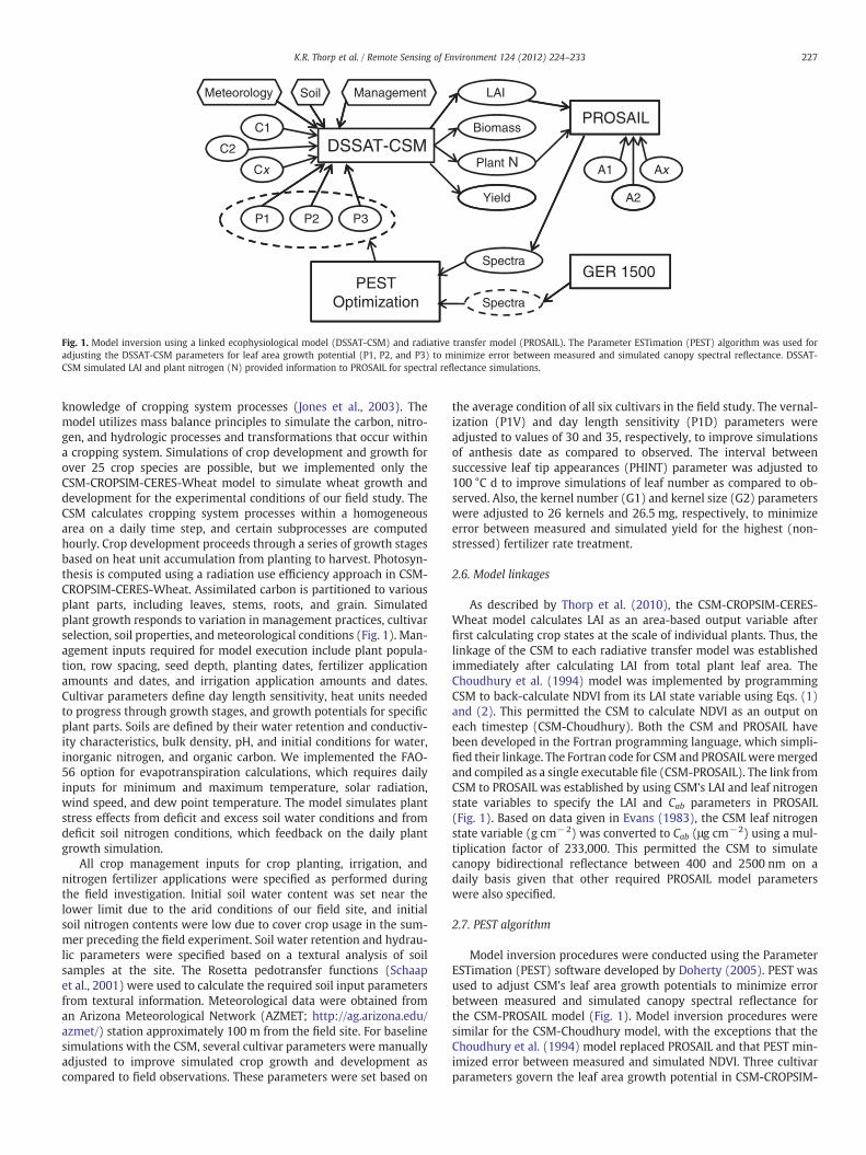
knowledge of cropping system processes (Jones et al., 2003). Themodel utilizes mass balance principles to simulate the carbon, nitro-gen, and hydrologic processes and transformations that occur withina cropping system. Simulations of crop development and growth forover 25 crop species are possible, but we implemented only theCSM-CROPSIM-CERES-Wheat model to simulate wheat growth anddevelopment for the experimental conditions of our field study. TheCSM calculates cropping system processes within a homogeneousarea on a daily time step, and certain subprocesses are computedhourly. Crop development proceeds through a series of growth stagesbased on heat unit accumulation from planting to harvest. Photosyn-thesis is computed using a radiation use efficiency approach in CSM-CROPSIM-CERES-Wheat. Assimilated carbon is partitioned to variousplant parts, including leaves, stems, roots, and grain. Simulatedplant growth responds to variation in management practices, cultivarselection, soil properties, and meteorological conditions (Fig. 1). Man-agement inputs required for model execution include plant popula-tion, row spacing, seed depth, planting dates, fertilizer applicationamounts and dates, and irrigation application amounts and dates.Cultivar parameters define day length sensitivity, heat units neededto progress through growth stages, and growth potentials for specificplant parts. Soils are defined by their water retention and conductiv-ity characteristics, bulk density, pH, and initial conditions for water,inorganic nitrogen, and organic carbon. We implemented the FAO-56 option for evapotranspiration calculations, which requires dailyinputs for minimum and maximum temperature, solar radiation,wind speed, and dew point temperature. The model simulates plantstress effects from deficit and excess soil water conditions and fromdeficit soil nitrogen conditions, which feedback on the daily plantgrowth simulation.

All crop management inputs for crop planting, irrigation, andnitrogen fertilizer applications were specified as performed duringthe field investigation. Initial soil water content was set near thelower limit due to the arid conditions of our field site, and initialsoil nitrogen contents were low due to cover crop usage in the sum-mer preceding the field experiment. Soil water retention and hydrau-lic parameters were specified based on a textural analysis of soilsamples at the site. The Rosetta pedotransfer functions (Schaapet al., 2001) were used to calculate the required soil input parametersfrom textural information. Meteorological data were obtained froman Arizona Meteorological Network (AZMET; http://ag.arizona.edu/azmet/) station approximately 100 m from the field site. For baselinesimulations with the CSM, several cultivar parameters were manuallyadjusted to improve simulated crop growth and development ascompared to field observations. These parameters were set based on

the average condition of all six cultivars in the field study. The vernal-ization (P1V) and day length sensitivity (P1D) parameters wereadjusted to values of 30 and 35, respectively, to improve simulationsof anthesis date as compared to observed. The interval betweensuccessive leaf tip appearances (PHINT) parameter was adjusted to100 °C d to improve simulations of leaf number as compared to ob-served. Also, the kernel number (G1) and kernel size (G2) parameterswere adjusted to 26 kernels and 26.5 mg, respectively, to minimizeerror between measured and simulated yield for the highest (non-stressed) fertilizer rate treatment.

2.6. Model linkages

As described by Thorp et al. (2010), the CSM-CROPSIM-CERES-Wheat model calculates LAI as an area-based output variable afterfirst calculating crop states at the scale of individual plants. Thus, thelinkage of the CSM to each radiative transfer model was establishedimmediately after calculating LAI from total plant leaf area. TheChoudhury et al. (1994) model was implemented by programmingCSM to back-calculate NDVI from its LAI state variable using Eqs. (1)and (2). This permitted the CSM to calculate NDVI as an output oneach timestep (CSM-Choudhury). Both the CSM and PROSAIL havebeen developed in the Fortran programming language, which simpli-fied their linkage. The Fortran code for CSM and PROSAILweremergedand compiled as a single executable file (CSM-PROSAIL). The link fromCSM to PROSAIL was established by using CSM's LAI and leaf nitrogenstate variables to specify the LAI and Cab parameters in PROSAIL(Fig. 1). Based on data given in Evans (1983), the CSM leaf nitrogenstate variable (g cm−2) was converted to Cab (μg cm−2) using a mul-tiplication factor of 233,000. This permitted the CSM to simulatecanopy bidirectional reflectance between 400 and 2500 nm on adaily basis given that other required PROSAIL model parameterswere also specified.

2.7. PEST algorithm

Model inversion procedures were conducted using the ParameterESTimation (PEST) software developed by Doherty (2005). PEST wasused to adjust CSM's leaf area growth potentials to minimize errorbetween measured and simulated canopy spectral reflectance forthe CSM-PROSAIL model (Fig. 1). Model inversion procedures weresimilar for the CSM-Choudhury model, with the exceptions that theChoudhury et al. (1994) model replaced PROSAIL and that PEST min-imized error between measured and simulated NDVI. Three cultivarparameters govern the leaf area growth potential in CSM-CROPSIM-

Meteorology ManagementSoil LAI

C1

C2 DSSAT-CSMCx

Biomass

Plant N

Yield

PROSAIL

A1

A2

Ax

P2 P3P1

PESTOptimization

SpectraGER 1500

Spectra

Fig. 1. Model inversion using a linked ecophysiological model (DSSAT-CSM) and radiative transfer model (PROSAIL). The Parameter ESTimation (PEST) algorithm was used foradjusting the DSSAT-CSM parameters for leaf area growth potential (P1, P2, and P3) to minimize error between measured and simulated canopy spectral reflectance. DSSAT-CSM simulated LAI and plant nitrogen (N) provided information to PROSAIL for spectral reflectance simulations.

227K.R. Thorp et al. / Remote Sensing of Environment 124 (2012) 224–233

CERES-Wheat, including the area of the standard first leaf (LA1S,cm2), the vegetative phase leaf area adjustment factor (LAFV), andthe reproductive phase leaf area adjustment factor (LAFR). We setPEST to optimize LA1S and LAFV, while LAFR was tied to LAFV suchthat their resulting optimized parameter values were identical. LA1Swas allowed to vary between 0.5 and 2.5 cm2. LAFV was allowed tovary from 0.01 to 3.00. Limits for these parameters were chosenusing a sensitivity analysis to assess their impact on simulated LAI.We also attempted to adjust other CSM parameters, such as theplant population, the potential specific leaf weight, the growth stagedurations, and the soil fertility factor. However, preliminary PESTresults demonstrated that the leaf area growth potentials were themost effective CSM parameters for this optimization problem. There-fore, we finally focused on optimizing only the three parameters thatdefine the leaf area growth: LA1S, LAFV, and LAFR.

2.8. Genetic algorithm

Inversion of the CSM-Choudhury and CSM-PROSAIL models andaccuracy of the estimated crop biophysical properties were expectedto be heavily influenced by the timing and availability of remote sens-ing observations. Field outings with the GER 1500 spectroradiometerresulted in 16 observations of canopy spectral reflectance in eachplot, which were collected on a near weekly basis. Observationswere available on the following days after planting: 30, 34, 42, 48,54, 61, 69, 71, 77, 83, 91, 97, 105, 113, 119, and 125. To assess theimpact of observation timing and availability, a genetic algorithmwas implemented to find the set of remote sensing observationsthat optimally estimated LAI through inversion of CSM-Choudhuryand CSM-PROSAIL. We focused on selecting the observations that op-timized LAI, because it was likely the most fundamental state variableaffected by adjusting the leaf area growth parameters during modelinversion.

To set up the genetic algorithm, a chromosome with 16 1-bitgenes was established, one gene for each remote sensing observationdate. Each bit indicated whether the remote sensing observation fromits respective date should or should not be included in the PEST opti-mization (Fig. 1). A two-point crossover method was used with acrossover rate of 0.90, and a bit flip mutation method was usedwith a mutation rate of 0.06. The population size was 47. For furtherconstraint, the algorithm was seeded with the optimum results ofmodel inversions based on all possible combinations of one, two,and three remote sensing observations. The algorithm was allowedto run for 100 generations, although the optimum set of remote sensingobservations was usually found within 5 generations. Results for CSM-Choudhury and CSM-PROSAIL are reported for the set of remote sensingobservations that achieved the optimum LAI simulation results.

To summarize, we used the genetic algorithm to select whichremote sensing observations to include in the model inversion proce-dure (Fig. 1). Actual adjustment of the model parameters to minimizeerror between measured and simulated NDVI or canopy spectralreflectance was accomplished with the PEST optimization algorithm,described in the previous section.

2.9. Analysis

The Choudhury et al. (1994) and PROSAIL radiative transfermodels provided a link between CSM-simulated LAI and canopy spec-tral reflectance, such that we could use model inversion to optimizeleaf area growth simulations based on remote sensing observationsof wheat canopy spectral reflectance. We assessed the value of thisapproach for estimating key crop biophysical properties, includingLAI, canopy weight, plant nitrogen content, and crop yield (Fig. 1).We also compared results between the linked models and theirstand-alone components. The following assessments were madeusing data for each treatment in the field study:

• Choudhury alone — The ζ and β parameters in the Choudhury et al.(1994) model were adjusted to minimize error between model-estimated and field-observed LAI. The NDVI was calculated by aver-aging GER 1500 canopy spectral reflectance observations within theLandsat TM wavebands for red (630 to 690 nm) and near-infrared(760 to 900 nm) radiation. This approach only provided an estimateof LAI.

• PROSAIL alone — PEST was implemented to invert the PROSAILmodel by adjusting the LAI and Cab parameters to minimize errorbetween simulated and observed canopy spectral reflectance from400 to 900 nm. This approach provided an estimate of LAI and Cab.

• CSM alone — Stand-alone CSM simulations provided baseline esti-mates for LAI, canopy weight, plant nitrogen content, and wheatyield without any PEST optimization. Only the manual parameteradjustments described previously were incorporated in these simu-lations. Leaf area growth potentials were left at default values, andthe model was not parameterized to simulate any cultivar differ-ences. Only fertilizer management differences were simulated.

• CSM-Choudhury — PEST was implemented to invert the CSM-Choudhury model by adjusting CSM's leaf area growth potentialsto minimize error between measured and simulated NDVI throughthe Choudhury et al. (1994) model linkage. Observed NDVI wascalculated by averaging the GER 1500 canopy spectral reflectanceobservations within the Landsat TM wavebands for red (630 to690 nm) and near-infrared (760 to 900 nm) radiation. The geneticalgorithmwas implemented to find the set of remote sensing obser-vations that optimally estimated LAI through model inversion.

• CSM-PROSAIL — PEST was implemented to invert the CSM-PROSAILmodel by adjusting CSM's leaf area growth potentials to minimizeerror between measured and simulated canopy spectral reflectanceobservations from 400 to 900 nm through the PROSAIL linkage(Fig. 1). The genetic algorithm was implemented to find the set ofremote sensing observations that optimally estimated LAI throughmodel inversion.

Results for LAI were evaluated by calculating the relative rootmean squared error (RRMSE) between measured and simulated LAIon dates with LAI-2000 Plant Canopy Analyzer measurements. Forcanopy weight and plant nitrogen content, the RRMSE between mea-sured and simulated values was calculated on biomass collectiondates. The RRMSE between measured and simulated yield was alsocomputed. The R statistical software (www.r-project.org) was usedto conduct an analysis of variance and Tukey's multiple comparisonstest on the optimized leaf area growth parameters resulting frominversion of CSM-Choudhury and CSM-PROSAIL.

3. Results and discussion

3.1. LAI observations

Since LAI was a key variable in this study, we measured it usingtwo field methods, one based on readings from the Li-Cor LAI-2000Plant Canopy Analyzer and the other based on processing of biomasssamples. A primary advantage of the Li-Cor LAImeterwas its relativelyquick and easymeasurement protocol, whereas processing of biomasssampleswas quite labor-intensive and time-consuming.Wewere ableto estimate LAI on a weekly basis with the Li-Cor LAI meter, whereasbiomass samples were collected and processed only four timesthroughout the growing season. Since the Li-Cor LAI data were moreplentiful, we used these data to evaluate the model simulations.Fig. 2 compares LAI observations from the Li-Cor meter and from bio-mass sampling for the four days when estimates of LAI from biomasssamples were available. The RMSE between LAI observations forthese two field methods was 0.52. We concluded that the Li-Cor LAI-2000 Plant Canopy Analyzer could reasonably estimate LAI and couldbe used for further evaluation of model simulations.

228 K.R. Thorp et al. / Remote Sensing of Environment 124 (2012) 224–233

3.2. Estimating LAI

Relationships betweenmeasured and simulated LAI for each of thefive modeling scenarios is given in Fig. 3. The stand-alone Choudhurymodel provided reasonable LAI estimates over the entire growingseason (Fig. 3a) with a 29.4% RRMSE between measured and modeledLAI (Table 3). Relative to the othermodeling scenarios, the Choudhuryet al. (1994) model performed well, although its usefulness is limitedonly to LAI estimation. The stand-alone PROSAIL model inversionperformed relatively poorly and had a tendency to overestimate LAIin the early season (LAIb2) and underestimate LAI in the mid to lateseason (LAI>2) (Fig. 3b). As corroborated by Botha et al. (2010), theoverestimation of LAI in the early season may be related to PROSAIL'sassumption of canopy homogeneity. The RRMSE between measuredand modeled LAI was 40.7% for PROSAIL alone (Table 3). Simulations

of LAI with the stand-alone CSM model were reasonable with aRRMSE of 27.8% (Table 3). However, the model tended to underesti-mate LAI observations between 1.5 and 2.5 (Fig. 3c). This issue wasremediated using remote sensing data to adjust the leaf area growthpotentials through the radiative transfer model linkages (Fig. 3dand e).

Simulations of LAI with the inverted CSM-Choudhury model weregood with a RRMSE of 24.8% (Table 3). Similar results were obtainedwith the inverted CSM-PROSAIL model, which estimated LAI with aRRMSE of 24.1%. Scatter plots of measured and simulated LAI fromboth the inverted CSM-Choudhury model and the inverted CSM-PROSAIL model fit well to the one-to-one line (Fig. 3d and e). Notably,the inversion of CSM-PROSAIL estimated LAI better than either CSMor PROSAIL alone. Likewise, the inversion of CSM-Choudhury estimat-ed LAI better than either CSM or the Choudhury model alone. Thisdemonstrated the usefulness of the linkages between the radiativetransfer and ecophysiological models. The temporal LAI simulationfrom CSM provided constraint to the PROSAIL model that was notavailable for inversions of PROSAIL alone. Likewise, PROSAIL providedthe physical model necessary for adjusting CSM's leaf area growthparameters based on canopy spectral reflectance information. To-gether, the models were able to estimate LAI with greater accuracythan either model alone.

3.3. Estimating canopy weight

Canopy weight was estimated with RRMSEs of 18.6%, 13.4%, and14.4% for the stand-alone CSM model, the CSM-Choudhury inversion,

0

1

2

3

4

5

6

0 1 2 3 4 5 6

LA

I fro

m L

i-C

or

LA

I-20

00

LAI from Biomass Samples

RMSE= 0.52

Fig. 2. Leaf area index (LAI) measured with the Li-Cor LAI-2000 Plant Canopy Analyzerversus the LAI estimated through processing of wheat biomass.

(a) (b) (c)

Mo

del

ed L

AI

(a) (b) (c)(a) (b) (c)(a) (b) (c)

(d) (e)

(a) (b) (c)

(d) (e)

Measured LAIMeasured LAI0 1 2 3 4 50 1 2 3 4 50 1 2 3 4 5

Measured LAI

0

1

2

3

4

5

Mo

del

ed L

AI

0

1

2

3

4

5 a) b) c)

d) e)

Fig. 3. Modeled versus measured leaf area index (LAI) for the a) Choudhury model alone, b) PROSAIL model alone, c) CSM alone, d) CSM-Choudhury linked model, and e) CSM-PROSAIL linked model.

Table 3Relative root mean squared error (%) between measured and modeled leaf area index(LAI), canopy weight (biomass), plant nitrogen (N), and wheat yield.

Choudhuryalone

PROSAILalone

CSMalone

CSM-Choudhury

CSM-PROSAIL

LAI 29.4 40.7 27.8 24.8 24.1Biomass – – 18.6 13.4 14.4Plant N – – 50.7 38.1 36.8Yield – – 12.8 12.4 10.0

229K.R. Thorp et al. / Remote Sensing of Environment 124 (2012) 224–233

and the CSM-PROSAIL inversion, respectively (Table 3). Again,inverting the linked radiative transfer and ecophysiological modelsprovided better estimates of canopy weight than simulations withCSM alone. The stand-alone CSM model used identical cultivar pa-rameters to simulate all the treatments in the study, as demonstratedby the lack of variability in modeled results (Fig. 4a). By using remotesensing data to adjust the leaf area growth parameters for eachunique treatment, we were able to account for cultivar differencesthat we did not simulate with CSM alone (Fig. 4b and c). The modelinversion proceduremay have also compensated for error in the spec-ification of applied fertilizer rates for each nitrogen treatment. Use ofremote sensing observations to adjust CSM's leaf growth parametersled to improved simulations of LAI (Fig. 3), and this improvementsubsequently led to better estimates of canopy weight (Fig. 4) eventhough canopy weight was not explicitly used to constrain the radia-tive transfer model (Fig. 1). This further highlights an advantage oflinking DSSAT-CSM with the radiative transfer models.

3.4. Estimating plant nitrogen content

Plant nitrogen contentwas simulatedwith RRMSEs of 50.7%, 38.1%,and 36.8% for the stand-alone CSMmodel, the CSM-Choudhury inver-sion, and the CSM-PROSAIL inversion, respectively (Table 3). Simula-tions of plant nitrogen content with the stand-alone CSM modelwere quite poor (Fig. 5), especially in the early growing seasonwhen observed plant nitrogen contents were greater than 2%. Simula-tions of plant nitrogen content tended to reach a minimum thresholdin the early season, which may be attributable to the tendency of thestand-alone CSM model to overestimate canopy weight at values lessthan 2 Mg ha−1 (Fig. 4a). Since plant nitrogen content is the ratio ofplant nitrogen mass over canopy weight, overestimation of canopyweight at a given level of nitrogen uptake resulted in a minimizationof plant nitrogen content. By using remote sensing data to adjust thesimulations of LAI, improvements in the canopy weight simulations

also improved themodel's ability to simulation plant nitrogen content(Fig. 5b and c).

The coefficient of determination (r2) between the leaf-level chlo-rophyll content (Cab) from stand-alone PROSAIL model inversionand field-measured plant-level nitrogen content was 0.07 (notshown). To assess the reason for this poor relationship, we comparedthe Cab from PROSAIL model inversion with the Cab calculated fromCSM-PROSAIL simulations of leaf nitrogen content using the relation-ship of Evans (1983). Results demonstrated an issue with the stand-alone PROSAIL model inversion procedure, similar to what has beenreported elsewhere (Jacquemoud et al., 1995). Approximately 20%of the PROSAIL model inversions resulted in an optimized Cab param-eter value of 150 μg cm−2 (Fig. 6), which was the upper limit im-posed for parameter optimization at outset. Increasing this upperlimit would result in optimized Cab parameter values much higherthan realistically anticipated. Decreasing the upper limit would likelycause a higher percentage of Cab parameter values to be optimized tothe upper limit value, which reduces the value of inverting PROSAIL.When inverting the linked CSM-PROSAIL model, the Cab parameterwas restrained by the physics of crop growth and nitrogen processescontained in the CSM. This resulted in Cab parameter values that weremore stable and realistic around 59 μg cm−2 (Fig. 6).

3.5. Estimating wheat yield

A primary benefit of the linkage between radiative transfer andecophysiological models is the ability to estimate (and ideally predict)crop yield based on remote sensing observations throughout the grow-ing season. Our results showed that the radiative transfer model link-ages did improve CSM simulations of wheat yield with RRMSEs of12.8%, 12.4%, and 10.0% for the stand-alone CSM model, the CSM-Choudhury inversion, and the CSM-PROSAIL inversion, respectively(Table 3). Since the stand-alone CSM model was calibrated for yieldsimulations of the highest, non-stressed nitrogen treatment,

(a) (b) (c)12

(a) (b) (c)

0

2

4

6

8

10

Mo

del

ed B

iom

ass

(Mg

ha-1

)

0 2 4 6 8 10 120 2 4 6 8 10 120 2 4 6 8 10 12Measured Biomass (Mg ha-1) Measured Biomass (Mg ha-1) Measured Biomass (Mg ha-1)

a) b) c)

Fig. 4. Modeled versus measured wheat canopy weight (above ground biomass) for the a) CSM alone, b) CSM-Choudhury linked model, and c) CSM-PROSAIL linked model.

(c)

(c)(c)(c)

(a) (b) (c)(c)

(c)(c)(c)

(a) (b) (c)(c)

(c)(c)(c)

(a) (b) (c)(c)

(c)(c)(c)

(a) (b) (c)(c)

(c)(c)(c)

(a) (b) (c)(c)

(c)(c)(c)

(a) (b) (c)

0

1

2

3

4

Mo

del

ed P

lan

t N

(%

) (c)

Measured Plant N (%)

(c)

Measured Plant N (%)

(c)

0 1 2 3 40 1 2 3 40 1 2 3 4Measured Plant N (%)

(c)

a) b) c)

Fig. 5. Modeled versus measured plant nitrogen (N) content for the a) CSM alone, b) CSM-Choudhury linked model, and c) CSM-PROSAIL linked model.

230 K.R. Thorp et al. / Remote Sensing of Environment 124 (2012) 224–233

improvements in yield estimation using the radiative transfer modellinkages were most apparent for the lower nitrogen rate treatments(Fig. 7). Improvements in the LAI simulation (Fig. 3), canopy weightsimulation (Fig. 4) and the plant nitrogen simulation (Fig. 5) byadjusting leaf area growth parameters using remote sensing observa-tions ultimately guided the model to improved simulations of wheatyield (Fig. 7).

3.6. Estimating leaf area growth potential

Further insights into the inversion of CSM-Choudhury and CSM-PROSAIL were obtained by analyzing the leaf area growth parametersresulting from PEST optimization. A common problem of model inver-sion is aberrant optimized parameter values that tend to remain at theupper or lower boundaries imposed at the outset (Jacquemoud et al.,1995). This can result in non-normal histograms, similar to thatobtained by inverting the stand-alone PROSAIL model to estimateCab (Fig. 6). Out of 60 model inversion exercises for CSM-Choudhuryand CSM-PROSAIL in this study (6 cultivars by 5 nitrogen rates foreach model), 7 (12%) resulted in an optimized leaf area growth pa-rameter remaining at an upper or lower bound. All of these 7 resultedfrom the initial leaf size parameter (LA1S, cm2) remaining at the lowerbound. Six of these occurred for CSM-PROSAIL model inversions at thelowest two nitrogen rates. The inversion procedure likely pushed theLA1S parameter down to account for growth reductions at the lowernitrogen rates.

Statistical analysis of the optimized parameter values demonstrat-ed differences depending on the wheat cultivar and nitrogen rate. ForCSM-Choudhury, there were differences in LAFV and LAFR among the

nitrogen rates (pb0.05); however, there were no differences in LA1S(Table 4). No differences were found for any of the three parametersamong the wheat cultivars. This means the inversion of CSM-Choudhury mainly adjusted for error in the nitrogen simulation rath-er than accounting for any cultivar differences. Highlighting theadded value of using the full canopy reflectance spectrum, the LAFVand LAFR parameters optimized for CSM-PROSAIL were statisticallydifferent among several of the wheat cultivars (pb0.05, Table 5). Dif-ferences in canopy spectral reflectance among the cultivars allowedthe inversion procedure to find unique parameters for Duraking andKronos cultivars as compared to Topper and Ocotillo. Given that weused the inversion procedure to adjust three cultivar parameters inthe model, the finding of statistically different parameters based oncrop cultivar is encouraging. However, no differences were found forthe LA1S parameter with CSM-PROSAIL. Among the nitrogen rates, allthree parameters showed differences with CSM-PROSAIL (pb0.05). Inparticular, parameters for the lowest and highest nitrogen rate treat-ments were statistically different for all three parameters.

Further statistical analysis focused on the combined set of optimizedparameters for CSM-Choudhury and CSM-PROSAIL. This showed statis-tically significant parameter values for LA1S, LAFV, and LAFR among thetwo model types (pb0.05, Table 6), and no statistical differences werefound between cultivars and nitrogen rates in this case. LA1S definesthe initial potential leaf size, whereas LAFV and LAFR define fractionalincrease in potential leaf size during the vegetative and reproductivegrowth phases, respectively. For CSM-Choudhury, the initial potentialleaf size was higher than for CSM-PROSAIL. However, the fractionalincrease in potential leaf size was higher for CSM-PROSAIL than forCSM-Choudhury. Thus, although the leaf potential size was initiallysmaller for CSM-PROSAIL, it had greater potential to increase as thegrowing season progressed. Although the model inversion procedureresulted in two different parameter sets for CSM-Choudhury and

0

5

10

15

20

25

30

35

40

45

20 30 40 50 60 70 80 90 100

110

120

130

140

150

160

Fre

qu

ency

(%

)

Leaf Chlorophyll Content (µg cm-2)

PROSAIL alone

CSM-PROSAIL

Fig. 6. Histogram of modeled chlorophyll a and b content for PROSAIL alone and for theCSM-PROSAIL linked model.

(a)(a)(a)(a)

(a) (b) (c)

0

2

4

6

Mo

del

ed Y

ield

(M

g h

a-1)

(a)(a)(a)(a)

(a) (b) (c)(a)

(a)(a)

0 2 4 6 80 2 4 6 80 2 4 6 8Measured Yield (Mg ha-1)Measured Yield (Mg ha-1)Measured Yield (Mg ha-1)

(a)

a) b) c)8

Fig. 7. Modeled versus measured wheat yield for the a) CSM alone, b) CSM-Choudhury linked model, and c) CSM-PROSAIL linked model.

Table 4Treatment means for the optimized leaf area growth parameters (LA1S, LAFV, andLAFR) from inversion of CSM-Choudhury. Letters indicate statistically significantgroups at the 0.05 significance level. Results for LAFV and LAFR are identical, becausewe linked these parameters in the PEST optimization.

LA1S LAFV LAFR

CultivarDuraking 1.228 a 0.330 a 0.330 aTopper 1.100 a 0.490 a 0.490 aKronos 1.289 a 0.368 a 0.368 aHavasu 0.931 a 0.491 a 0.491 aOrita 1.034 a 0.445 a 0.445 aOcotillo 1.142 a 0.496 a 0.496 a

Nitrogen rateN1 1.318 a 0.249 a 0.249 aN2 1.067 a 0.374 ab 0.374 abN3 1.281 a 0.435 abc 0.435 abcN4 0.995 a 0.534 bc 0.534 bcN5 0.942 a 0.593 c 0.593 c

231K.R. Thorp et al. / Remote Sensing of Environment 124 (2012) 224–233

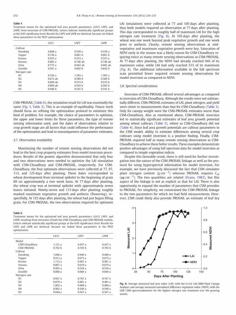
CSM-PROSAIL (Table 6), the simulation result for LAI was essentially thesame (Fig. 3, Table 3). This is an example of equifinality. Future workshould focus on refining the optimization protocol to minimize thiskind of problem. For example, the choice of parameters to optimize,the upper and lower limits for these parameters, the type of remotesensing information used, and the dates of observations relative tocrop growth stage are all factors that could influence the performanceof the optimization and lead to nonuniqueness of parameter estimates.

3.7. Observation availability

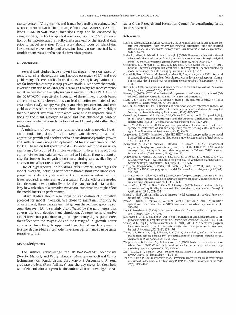
Maximizing the number of remote sensing observations did notlead to the best crop property estimates from model inversion proce-dures. Results of the genetic algorithm demonstrated that only fourand two observations were needed to optimize the LAI simulationwith CSM-Choudhury and CSM-PROSAIL, respectively. For CSM-Choudhury, the four optimum observations were collected at 77, 97,113, and 125 days after planting. These dates corresponded towheat development from terminal spikelet to the beginning of grainfill on approximately a two week basis. At 77 days after planting,the wheat crop was at terminal spikelet with approximately sevenleaves initiated. Ninety-seven and 113 days after planting roughlymarked maximum vegetative growth and anthesis (flowering), re-spectfully. At 125 days after planting, the wheat had just begun fillinggrain. For CSM-PROSAIL, the two observations required for optimum

LAI simulations were collected at 77 and 105 days after planting,thus both models required an observation at 77 days after planting.This day corresponded to roughly half of maximum LAI for the highnitrogen rate treatment (Fig. 8). At 105 days after planting, thewheat was one week beyond peak vegetative growth and one weekprior to anthesis. Clearly, remote sensing observations at mid-vegetative and maximum vegetative growth were key. Saturation ofNDVI early in the season was a likely reason for CSM-Choudhury re-quiring twice as many remote sensing observations as CSM-PROSAIL.At 77 days after planting, the NDVI had already reached 94% of itsmaximum value, while LAI had only reached 51% of its maximum(Fig. 8). The additional information available in the full spectrumscan permitted fewer required remote sensing observations formodel inversion as compared to NDVI.

3.8. Spectral considerations

Inversion of CSM-PROSAIL offered several advantages as comparedto inversion of CSM-Choudhury. Although the results were not substan-tially different, CSM-PROSAIL estimates of LAI, plant nitrogen, and yieldwere closer to measurements than that for CSM-Choudhury (Table 3).Only for canopy weight were the CSM-PROSAIL estimates worse thanCSM-Choudhury. Also as mentioned above, CSM-PROSAIL inversionled to statistically significant estimates of leaf area growth potentialamong wheat cultivars (Table 5), where as CSM-Choudhury did not(Table 4). Since leaf area growth potentials are cultivar parameters inthe CSM model, ability to estimate differences among several cropcultivars using model inversion is a positive finding. Finally, CSM-PROSAIL required half as many remote sensing observations as CSM-Choudhury to achieve these better results. These examples demonstratepositive advantages of using full spectrum data for model inversion ascompared to simple vegetation indices.

Despite this favorable result, there is still need for further investi-gation into the nature of the CSM-PROSAIL linkage as well as the pro-tocol for using hyperspectral information for model inversion. Forexample, we have previously discussed the fact that CSM simulatesplant nitrogen content (g cm−2) whereas PROSAIL requires Cab(μg cm−2). The two quantities are related (Evans, 1983), but thisaspect of the linkage is not as explicit as that for LAI. There is alsoopportunity to expand the number of parameters that CSM providesto PROSAIL. For simplicity, we constrained the CSM-PROSAIL linkageto the two parameters for which we had field measurements. How-ever, CSM could likely also provide PROSAIL an estimate of leaf dry

Table 5Treatment means for the optimized leaf area growth parameters (LA1S, LAFV, andLAFR) from inversion of CSM-PROSAIL. Letters indicate statistically significant groupsat the 0.05 significance level. Results for LAFV and LAFR are identical, because we linkedthese parameters in the PEST optimization.

LA1S LAFV LAFR

CultivarDuraking 0.868 a 0.550 a 0.550 aTopper 0.726 a 0.861 b 0.861 bKronos 0.935 a 0.553 a 0.553 aHavasu 0.683 a 0.746 ab 0.746 abOrita 0.772 a 0.662 ab 0.662 abOcotillo 0.591 a 0.842 b 0.842 b

Nitrogen rateN1 0.536 a 1.285 a 1.285 aN2 0.672 ab 0.589 b 0.589 bN3 0.849 ab 0.533 b 0.533 bN4 0.809 ab 0.565 b 0.565 bN5 0.946 b 0.541 b 0.541 b

Table 6Treatment means for the optimized leaf area growth parameters (LA1S, LAFV, andLAFR) resulting from inversion of both the CSM-Choudhury and CSM-PROSAIL models.Letters indicate statistically significant groups at the 0.05 significance level. Results forLAFV and LAFR are identical, because we linked these parameters in the PESToptimization.

LA1S LAFV LAFR

ModelCSM-Choudhury 1.121 a 0.437 a 0.437 aCSM-PROSAIL 0.762 b 0.703 b 0.703 b

CultivarDuraking 1.048 a 0.440 a 0.440 aTopper 0.913 a 0.675 a 0.675 aKronos 1.112 a 0.461 a 0.461 aHavasu 0.807 a 0.619 a 0.619 aOrita 0.903 a 0.554 a 0.554 aOcotillo 0.866 a 0.669 a 0.669 a

Nitrogen rateN1 0.927 a 0.767 a 0.767 aN2 0.870 a 0.481 a 0.481 aN3 1.065 a 0.484 a 0.484 aN4 0.902 a 0.549 a 0.549 aN5 0.944 a 0.567 a 0.567 a

LAI

NDVI

0.0

0.2

0.4

0.6

0.8

1.0

0

1

2

3

4

25 50 75 100 125 150

Mea

sure

d N

DV

I

Mea

sure

d L

AI

Days After Planting

LAI

NDVI

Fig. 8. Average measured leaf area index (LAI) with the Li-Cor LAI-2000 Plant CanopyAnalyzer and average measured normalized difference vegetation index (NDVI) with theGER 1500 spectroradiometer for the highest nitrogen rate treatment over the growingseason.

232 K.R. Thorp et al. / Remote Sensing of Environment 124 (2012) 224–233

matter content (Cm; g cm−2), and it may be possible to estimate leafwater content or leaf inclination angle from CSM's water stress simu-lation. CSM-PROSAIL model inversions may also be enhanced byusing a strategic subset of spectral wavelengths in the PEST optimiza-tion or by incorporating a multivariate analysis of the spectral dataprior to model inversion. Future work should focus on identifyingkey spectral wavelengths and assessing how various spectral bandcombinations would influence the inversion process.

4. Conclusions

Several past studies have shown that model inversion based onremote sensing observations can improve estimates of LAI and cropyield. Many of these studies focused on using simple vegetation indi-ces for inversion of simple crop growth models. We show that modelinversion can also be advantageous through linkages of more complexradiative transfer and ecophysiological models, such as PROSAIL andthe DSSAT-CSM respectively. Inversion of these linked models basedon remote sensing observations can lead to better estimates of leafarea index (LAI), canopy weight, plant nitrogen content, and cropyield as compared to either model alone. In particular, we highlightthat our model inversion approaches were able to improve simula-tions of the plant nitrogen balance and leaf chlorophyll content,since most earlier studies have focused on LAI and yield rather thannitrogen.

A minimum of two remote sensing observations provided opti-mum model inversions for some cases. One observation at mid-vegetative growth and another betweenmaximum vegetative growthand anthesis was enough to optimize LAI for the inversion of CSM-PROSAIL based on full spectrum data. However, additional measure-ments may be required if simpler vegetation indices are used. Sinceour remote sensing data set was limited to 16 dates, there is opportu-nity for further investigation into how timing and availability ofobservations affect the model inversion performance.

Use of hyperspectral observations offers several advantages formodel inversion, including better estimation of most crop biophysicalproperties, statistically different cultivar parameter estimates, andfewer required remote sensing observations. Further efforts are neededto understand how to optimally utilize the hyperspectral data, particu-larly how selection of alternative waveband combinations might affectthe model inversion performance.

Future studies should also focus on exploration of alternativeprotocol for model inversion. We chose to maintain simplicity byadjusting only three parameters that govern the leaf area growth pro-cess. However, LAI is certainly also affected by the parameters thatgovern the crop development simulation. A more comprehensivemodel inversion procedure might independently adjust parametersthat affect both the magnitude and the timing of LAI growth. Betterapproaches for setting the upper and lower bounds on these parame-ters are also needed, since model inversion performance can be quitesensitive to this.

Acknowledgments

The authors acknowledge the USDA-ARS-ALARC technicians(Suzette Maneely and Kathy Johnson), Maricopa Agricultural Centertechnicians (Ken Randolph and Cory Runyon), University of Arizonagraduate student (Ruth Asiimwe), and the day crews for their helpwith field and laboratory work. The authors also acknowledge the Ar-

izona Grain Research and Promotion Council for contributing fundsfor this research.

References

Botha, E., Leblon, B., Zebarth, B., &Watmough, J. (2007). Non-destructive estimation of po-tato leaf chlorophyll from canopy hyperspectral reflectance using the invertedPROSAIL model. International Journal of Applied Earth Observation and Geoinformation,9(4), 360–374.

Botha, E., Leblon, B., Zebarth, B., & Watmough, J. (2010). Non-destructive estimation ofwheat leaf chlorophyll content from hyperspectral measurements through analyticalmodel inversion. International Journal of Remote Sensing, 31(7), 1679–1697.

Choudhury, B. J., Ahmed, N. U., Idso, S. B., Reginato, R. J., & Daughtry, C. S. T. (1994).Relations between evaporation coefficients and vegetation indexes studied bymodel simulations. Remote Sensing of Environment, 50(1), 1–17.

Combal, B., Baret, F., Weiss, M., Trubuil, A., Macé, D., Pragnère, A., et al. (2003). Retrievalof canopy biophysical variables from bidirectional reflectance using prior informa-tion to solve the ill-posed inverse problem. Remote Sensing of Environment, 84(1),1–15.

Davies, E. (2009). The application of machine vision to food and agriculture: A review.Imaging Science Journal, 57(4), 197–217.

Doherty, J. (2005). PEST: Model-independent parameter estimation User manual (5thedition). Brisbane, Australia: Watermark Numerical Computing.

Evans, J. R. (1983). Nitrogen and photosynthesis in the flag leaf of wheat (Triticumaestivum L.). Plant Physiology, 72, 297–302.

Goel, N., & Strebel, D. (1983). Inversion of vegetation canopy reflectance models forestimating agronomic variables. I. Problem definition and initial results using theSuits model. Remote Sensing of Environment, 13(6), 487–507.

Green, R. O., Eastwood, M. L., Sarture, C. M., Chrien, T. G., Aronsson, M., Chippendale, B. J.,et al. (1998). Imaging spectroscopy and the Airborne Visible/Infrared ImagingSpectrometer (AVIRIS). Remote Sensing of Environment, 65(3), 227–248.

Guerif, M., & Duke, C. L. (2000). Adjustment procedures of a crop model to the sitespecific characteristics of soil and crop using remote sensing data assimilation.Agriculture Ecosystems & Environment, 81(1), 57–69.

Jacquemoud, S. (1993). Inversion of the PROSPECT + SAIL canopy reflectance modelfrom AVIRIS equivalent spectra: Theoretical study. Remote Sensing of Environment,44(2–3), 281–292.

Jacquemoud, S., Baret, F., Andrieu, B., Danson, F., & Jaggard, K. (1995). Extraction ofvegetation biophysical parameters by inversion of the PROSPECT+SAIL modelson sugar beet canopy reflectance data. Application to TM and AVIRIS sensors.Remote Sensing of Environment, 52(3), 163–172.

Jacquemoud, S., Verhoef, W., Baret, F., Bacour, C., Zarco Tejada, P. J., Asner, G. P., et al.(2009). PROSPECT + SAIL models: A review of use for vegetation characterization.Remote Sensing of Environment, 113(Suppl. 1), S56–S66.

Jones, J. W., Hoogenboom, G., Porter, C. H., Boote, K. J., Batchelor, W. D., Hunt, L. A., et al.(2003). The DSSAT cropping systemmodel. European Journal of Agronomy, 18(3–4),235–265.

Koetz, B., Baret, F., Poilvé, H., & Hill, J. (2005). Use of coupled canopy structure dynamicand radiative transfer models to estimate biophysical canopy characteristics. Re-mote Sensing of Environment, 95(1), 115–124.

Luo, Y., Weng, E., Wu, X., Gao, C., Zhou, X., & Zhang, L. (2009). Parameter identifiability,constraint, and equifinality in data assimilation with ecosystem models. EcologicalApplications, 19(3), 571–574.

Maas, S. J. (1988). Using satellite data to improvemodel estimates of crop yield. AgronomyJournal, 80(4), 655–662.

Prevot, L., Chauki, H., Troufleau, D.,Weiss, M., Baret, F., & Brisson, N. (2003). Assimilatingoptical and radar data into the STICS crop model for wheat. Agronomie, 23(4),297–303.

Reda, I., & Andreas, A. (2004). Solar position algorithm for solar radiation applications.Solar Energy, 76(5), 577–589.

Rodriguez, J., Ustin, S., & Riaño, D. (2011). Contributions of imaging spectroscopy to im-prove estimates of evapotranspiration. Hydrological Processes, 25(26), 4069–4081.

Schaap, M. G., Leij, F. J., & van Genuchten, M. T. (2001). ROSETTA: A computer programfor estimating soil hydraulic parameters with hierarchical pedotransfer functions.Journal of Hydrology, 251(3–4), 163–176.

Thorp, K. R., Hunsaker, D. J., & French, A. N. (2010). Assimilating leaf area index esti-mates from remote sensing into the simulations of a cropping systems model.Transactions of the ASABE, 53(1), 251–262.

Wiegand, C. L., Richardson, A. J., & Kanemasu, E. T. (1979). Leaf area index estimates forwheat from LANDSAT and their implications for evapotranspiration and cropmodeling. Agronomy Journal, 71(2), 336–342.

Xie, Y. C., Sha, Z. Y., & Yu, M. (2008). Remote sensing imagery in vegetation mapping: Areview. Journal of Plant Ecology, 1(1), 9–23.

Yang, Y., & Ling, P. (2004). Improved model inversion procedure for plant water statusassessment under artificial lighting using PROSPECT+SAIL. Transactions of the ASAE,47(5), 1833–1840.

233K.R. Thorp et al. / Remote Sensing of Environment 124 (2012) 224–233