Estimating Dynamic Traffic Matricesby using Viable Routing Changes

Augustin Soule1, Antonio Nucci2, Rene Cruz3, Emilio Leonardi4, Nina Taft51 Thomson Research, Paris, France. 2 Narus Inc. Mountain View, CA. 3 University of California San Diego, CA.

4 Politecnico di Torino, Turin, Italy 5 Intel Research, Berkeley, CA.

Abstract— In this paper we propose a new approach for dealingwith the ill-posed nature of traffic matrix estimation. We presentthree solution enhancers: an algorithm for deliberately changinglink weights to obtain additional information that can make theunderlying linear system full rank; a cyclo-stationary model tocapture both long-term and short-term traffic variability, and amethod for estimating the variance of origin-destination (OD)flows. We show how these three elements can be combinedinto a comprehensive traffic matrix estimation procedure thatdramatically reduces the errors compared to existing methods.We demonstrate that our variance estimates can be used toidentify the elephant OD flows, and we thus propose a variantof our algorithm that addresses the problem of estimating onlythe heavy flows in a traffic matrix. One of our key findingsis that by focusing only on heavy flows, we can simplify themeasurement and estimation procedure so as to render it morepractical. Although there is a tradeoff between practicality andaccuracy, we find that increasing the rank is so helpful that wecan nevertheless keep the average errors consistently below the10% carrier target error rate. We validate the effectiveness ofour methodology and the intuition behind it using commercialtraffic matrix data from Sprint’s Tier-1 backbone.

Index Terms— Network Tomography, Traffic Matrix Estima-tion, Traffic Engineering, SNMP.

I. INTRODUCTION

A traffic matrix is a representation of the volume of trafficthat flows between origin-destination (OD) node pairs in anetwork. In the context of the Internet, the nodes can representPoints-of-Presence (PoPs), routers or links. In current IPbackbone networks, obtaining accurate estimates of trafficmatrices is problematic. There are a number of importanttraffic engineering tasks that could be greatly improved withthe knowledge provided by traffic matrices. As a result, net-work operators have identified a need for the development ofpractical methods to obtain accurate estimates of traffic matri-ces. Example applications of traffic matrix estimation includelogical topology design, capacity planning and forecasting,routing protocol configuration, provisioning for Service LevelAgreement (SLAs), load balancing, and fault diagnosis.

Direct measurement of traffic matrices across an entire ISPnetwork is considered too cumbersome in terms of com-munication and computation overhead to be practical withthe current state of the art flow monitoring equipment [7].Research in this area has thus turned to statistical inferencetechniques. The basic problem these techniques are applied to

This work was done when A. Nucci and N. Taft were at Sprint Labs.

is the following. The relationship between the traffic matrix,the routing and the link counts can be described by a systemof linear equations Y = AX , where Y is the vector of linkcounts, X is the traffic matrix organized as a vector, and Adenotes a routing matrix in which element aij is equal to 1 ifOD pair j traverses link i or zero otherwise. The elements{aij} take on values {0, 1} when traffic splitting is notallowed, but can take on fractional values when traffic splittingis supported. In networking environments today, Y and A arereadily available; the link counts Y can be obtained throughstandard SNMP measurements and the routing matrix A canbe obtained by examining IGP link weights together with thecorresponding topological information. The problem at handis to estimate the traffic matrix X . This is not straightforwardbecause the matrix A does not have full rank, and hence thefundamental problem is that of a highly under-constrained, orill-posed, system.

A first generation of techniques were proposed in [1], [2],[3]. Model parameters are estimated using either MomentGenerating methods [1], Bayesian methods [2] or MaximumLikelihood estimation [3]. A common idea behind theseapproaches to tackle the highly under-constrained problemwas to introduce additional constraints related to the secondorder moment of the OD pairs. Estimation is then carriedout with two batches of constraints, one on the first ordermoment and one batch for the second order moment. Howeverthe combined set of constraints is not solvable without anassumption on the relationship between the mean and variance.For example, in [1], [2] the authors assume that the volumeof traffic for a given OD pair has a Poisson distribution,thus with an identical mean and variance. Cao et al. [3]assume instead that the traffic volume for OD pairs followsa Gaussian distribution, and that a power law relationshipbetween the mean and variance exists. A comparative studyof these methods [4] revealed that these methods were highlydependent upon the initial starting point, often called a prior,of the estimation procedure. Hence a second generation oftechniques emerged [4], [5], [6] that proposed various methodsfor generating intelligent priors.

In practice, all of these statistical inference techniques forestimating traffic matrices suffer from limited accuracy. Themagnitude of estimation errors are distributed over a range,however in short we can say that the errors typically fallbetween 10 and 25%. Also these methods yield outliers suchthat some OD pairs can have errors above 100%. It has been

TO APPEAR IN IEEE/ACM TRANSACTION ON NETWORKING, AUGUST 2007 2

difficult to drive the estimation error down below these values.Some carriers have indicated that they would not use trafficmatrices for traffic engineering unless the inference methodscould drive the average errors below the 10% target.

The fundamental difficulty in the traffic matrix (TM) estima-tion problem is due to it being under-constrained. The naturalquestion to ask is whether or not there is anything we can doto increase the rank of the underlying linear system. In thiswork we propose the idea of deliberating changing the linkweights so as to alter the shortest path routes used betweeningress and egress nodes. The idea is by that doing this andcollecting new SNMP link measurements under these alteredrouting states, we collect more measurements that are linearlyindependent of the existing measurements, thereby increasingthe rank of the basic system Y = AX . In order to do this, analgorithm is needed to select which weights to change and byhow much their values should be altered [9].

Such an algorithm cannot be used alone to create a solutionto the TM problem because it would lead to a solution that isneither complete nor practical. The solution is not completebecause the routing configuration changes would have to beapplied over a multi-hour period (discussed below). The trafficitself during such time periods is non-stationary and thus theunderlying traffic model used in the inference solution needsto be able to capture long-term traffic behaviors. The solutionmay not be practical because carriers want to conduct a limitednumber of such routing configuration changes to avoid furthercomplicating the management of commercial networks. In thispaper, we develop a methodology for traffic matrix estimationsolution that resolves both of these problems.

Our methodology leads to two algorithms, the first allowsone to estimate all the OD flows in a traffic matrix with highaccuracy by combining cyclo-stationary models with routingchanges. The second algorithm yields a method for estimatingonly the elephant flows in a traffic matrix. This can be donewith very few routing changes thus rendering the methodpractical while maintaining good accuracy. A comparison ofthese two methods illustrates the tradeoff between practicality(limited routing changes) and accuracy.

Our contributions are multiple.• We propose the idea of changing routing configurations inorder to increase the rank of the linear system used for trafficmatrix estimation. This reduces the inherent ill-posed natureof the basic problem.• We provide an identifiability result for a TM estimationmethod that incorporates route changes. We prove that the firstorder moment of the OD flows is always identifiable undera proper sequence of routing configuration changes for anybidirectional biconnected topology. In other words, it is alwayspossible to obtain a full rank system for such a topology.• We develop a new model for OD flows that captures theirbehavior over long time periods (e.g., multiple hours or days).This enables traffic matrix estimation methods that may take along time to collect all the data needed to estimate accurately.Our OD flow model contains two critical components, diurnalpatterns that capture (long-term) cyclo-stationary behavior anda fluctuations process capturing short-term variability.

• We derive a closed form solution to estimate the covarianceof the TM based on our underlying OD models. To the bestof our knowledge, this is the first time that an estimate forthe covariance of a TM has been proposed. We also provethat under certain conditions the variance will always beidentifiable, i.e., that a unique solution exists.• We explain how to incorporate our three solution enhance-ments (route changes, cyclo-stationary models and varianceestimators) into a complete traffic matrix estimation methodol-ogy. Depending upon how these enhancements are combined,our methodology yields two different solutions, one for es-timating the entire traffic matrix and one for estimating theelephant OD flows only. By switching the goal (and solution)to focus only on heavy OD pairs we render our solutions morepractical. This is because with fewer variables to estimate,fewer weight changes are needed and less data needs to becollected. By incorporating the well accepted idea, that tinyflows are unimportant for most traffic engineering tasks intoour methods, we show how TM estimation can be simplifiedwhile retaining accurate estimates of the heavy flows.• We propose the first method that does not require anassumption about the relationship between the mean and thevariance of OD flows.

With our methods we can drive the average error rates downinto a whole new range, namely below the 10% target; andoften we reach 4 or 5% average error rates (depending uponthe scenario). To the best of our knowledge, this is the firstpaper that consistently achieves errors below this 10% barrier.

Our composite solution to the traffic matrix estimationproblem involves many elements. Part 1 of our solution waspresented in [9] where we first proposed the idea of changinglink weights so as to increase the rank of the system. In thatpaper we showed that the problem of finding a minimal setof link weight changes to achieve full rank is NP-hard andwe provided a heuristic algorithm for determining which linksare most advantageous to change and by how much a weightvalue should be altered. Part 2 of our solution appeared in[10], that presents our cyclo-stationary models, the varianceestimator, and explains how the models and routing changesare incorporated into a traffic matrix estimation procedure.In this journal version of our work, we present (in a singlepaper) the entire methodology (derived from the previoustwo papers), with a more comprehensive perspective. Todo this we include all the steps of the methods, includingthe Viable Routing Changes algorithm (VRC-heuristic), forcompleteness. However we have removed some discussions onsubtle points, examples illustrating the effect of steps in theweight change selection algorithm, and so on. This journalversion also differs from the previous two papers in that itcontains our result on identifiability of the first order moment,which has never been presented before.

II. PROBLEM STATEMENT

The network traffic demand estimation problem can beformulated as follows. Consider a network represented bya collection V = {1, 2, . . . , V } of nodes, and a set of Ldirected links L ⊂ V × V . Each node represents a set of

TO APPEAR IN IEEE/ACM TRANSACTION ON NETWORKING, AUGUST 2007 3

co-located routers (PoP). Each link represents an aggregate oftransmission resources between two PoPs. (We assume thereare no self directed links, e.g. there are no links l of the forml = (i, i).) We consider a finite time horizon consisting of Kdisjoint measurement intervals, indexed by k ∈ [0, ...,K − 1].We refer to each measurement interval as a snapshot. In eachsnapshot we change the link weights, i.e. the paths followedfor some OD pairs, and this gives a different image of ODpairs traversing the network. We assume the routing remainsunchanged within the same snapshot, while two differentsnapshots are characterized by two different routing scenarios.Within each snapshot, we collect multiple consecutive readingsof the link counts using the SNMP protocol at discrete time n,indexed from 0 to Ns−1. Each reading constitutes one sample.Each snapshot lasts for Ns×5 minutes because SNMP reportslink counts every 5 minutes.

Consider an origin destination (OD) pair p = (v1, v2), withv1 6= v2, where v1 denotes a traffic source (ingress node) andv2 denotes a traffic sink (egress node). Let Xp(k, n) be theamount of traffic associated with OD pair p (i.e., originatingat node v1 and departing the network at node v2) duringmeasurement interval k at discrete time n. We assume thatthe measurement intervals are long enough so we can ignoreany traffic stored in the network. Let P denote the set of allOD pairs; there are a total of |P| = P = V 2− V OD pairs. 1

We order the OD pairs p and form a column vector X(k, n)whose components are Xp(k, n) in some pre-defined order.

Let Yl(k, n) be the total volume of traffic that crosses linkl ∈ L during measurement interval k at time n. Y (k, n)represents the column vector whose components are Yl(k, n)for all l ∈ L. Let Al,p(k) be the fraction of the traffic Xp(k, n)from OD pair p that traverses link l during measurementinterval k at time n. Thus, Yl(k, n) =

∑p∈P Al,p(k)Xp(k, n).

Forming the L×P matrix A(k) with elements {Al,p(k)}, wehave in matrix notation

Y (k, n) = A(k)X(k, n) , ∀k ∈ [0,K−1] and n ∈ [0, Ns−1].(1)

In the literature, the Y (k, n) vector is called the link countvector, while A(k) is called the routing matrix. In IP networks,the routing matrix A(k) during each measurement intervalk can be obtained by gathering topological information, aswell as OSPF or ISIS link weights. Link counts Y (k, n) areobtained from SNMP data.

A general problem considered in the literature is to computean estimate of the traffic matrix X(k, n) for each k and ngiven the observed link count vectors Y (k, n) for each k andn, assuming that the routing matrix A(k) does not change intime, i.e. A(k1) = A(k2)∀k ∈ [0, K − 1], and that X(k, n)is a sample of a stationary (vector valued) random process.Furthermore it is generally assumed in prior work that thecomponents of X(k, n) are uncorrelated. The general problemis non-trivial since the rank of A(k) is at most L and L << P ,i.e. for each k the system of equations (1) is under-determined.

1In our analysis we neglect local traffic, i.e., traffic that enters and leavesthe network at the same node, since it does not contribute to the load on anyinter-PoP link.

The problem we consider in this paper is broader becausewe will allow the routing to change, so that we may indeedhave A(k1) 6= A(k2), and we will consider the case whenX(k, n) does not come from a stationary process.

III. ROUTE CHANGES

We now explain, via an example, why the idea of changingthe routing can help increase the rank of the system.

A. Essence of the Idea

A

B

C

ED

3 5

2

2

6

5

2

2

5

6

3A

B

C

ED

Snapshot 0 Snapshot 1

3

Fig. 1. Example: Impact of Routing Changes

Consider the network shown in Fig. 1 composed of fivenodes interconnected by six unidirectional links. Each link hasan associated weight and the traffic from each OD pair isrouted along the shortest cost path. For simplicity, we consideronly five OD pairs (indicated by arrows). On the left of Fig. 1we represent the network in its normal state, when no linkweight changes have been effected. Snapshot 0 would generatethe following system of linear equations.

YAB

YAD

YBD

YBC

YEC

YDE

=

1 1 0 0 00 0 1 0 00 0 0 0 00 1 0 1 00 0 0 0 10 0 1 0 0

XAB

XAC

XAE

XBC

XEC

The rank of routing matrix A(0) is four. Two of the five ODpairs ((A, E) and (E, C)) can be estimated exactly becausein this simple example they do not share their links withother OD pairs. On the right of Fig. 1 we show the effectof decreasing the weight of link l = (A,D) from 5 to 3(snapshot k = 1). This perturbation in the weights causesthe re-routing of the OD pair (A,C) through the new path{(A,D), (D,E), (E, C)}. This snapshot generates a new sys-tem of linear equations, i.e. a new routing matrix A(1), that canbe appended to the previous set. One line of the new routingmatrix would look like YAB = [1 0 0 0 0] [XAB ...]T .We can see that adding this to the original system of equationsadds a new linearly independent equation into the system. Asa consequence, the new system [A(0)T A(1)T ]T is full rankand all five OD pairs can be estimated exactly.

TO APPEAR IN IEEE/ACM TRANSACTION ON NETWORKING, AUGUST 2007 4

B. Identifiability of First Order Moment

In this section we prove that the first order moment problemis always identifiable under a proper sequence of routing con-figuration changes for any bidirectional biconnected topology,i.e. it is always possible to select a proper sequence of routingconfigurations to obtain a full rank aggregate routing matrixA.

v2

v3

v4

v0 v1

v5v6

εM

M

M

MM

11

1

1

11

v0

v3

v4

v5v6

v2

v1εε

11

1

1

11

M

M

MM

V−1−ε

v2

v3

v4

v0 v1

v5v6

v2

v3

v4

v0 v1

v5v6

1

1

1

11

1

1

11

V−2−2εε

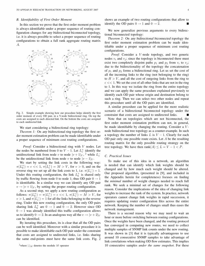
Fig. 2. Simple example showing how our procedure helps identify the firstorder moment of every OD pair, in a V-node bidirectional ring. On top thecosts are assigned to each directed link. On the bottom the costs are assignedto each undirected link.

We start considering a bidirectional ring topology:Theorem 1: On any bidirectional ring topology the first or-

der moment estimation problem can be made identifiable undera proper sequence of minimum cost routing configurations.

Proof: Consider a bidirectional ring with V nodes. Letthe nodes be numbered from 0 to V − 1. Let L+

v identify theunidirectional link from node v to node |v + 1|V , 2 while L−vbe the unidirectional link from node v to node |v − 1|V .

We start by setting the link costs in the following way:π(L+

0 ) = ε << 1, π(L+v ) = M > V , for v > 0, and on the

reverse ring we set up all the link costs to 1, i.e. π(L−v ) = 1.Under this routing configuration, the link L+

0 is shared onlyby traffic flowing from node 0 to node 1; thus OD pair 0 → 1is identifiable. In a similar way we can identify any OD pairv → |v + 1|V , by setting the proper routing configuration.

As a second step, we apply a new routing configuration asfollows: π(L+

0 ) = π(L+1 ) = ε << 1, π(L+

v ) = M > V , forv > 1, and π(L−v ) = 1 for all the links belonging to the reversering. Under this new routing configuration, the only OD pairssharing link L+

0 are 0 → 1 and 0 → 2. However since OD0 → 1 was already identified this traffic configuration allowsus to identify 0 → 2. In an analogous way all the v → |v + 2|Vcan be identified.

By iterating this procedure, its is clear that all the OD pairscan be well identified. Moreover with a similar procedure it ispossible to make identifiable each OD pair under the constraintthat costs are assigned to undirected links, i.e. links sharingthe same end-points must have the same link costs. Fig. 2

2where |.|M denotes the module M operator

shows an example of two routing configurations that allow toidentify the OD pairs 0 → 1 and 0 → 2.

We now generalize previous arguments to every bidirec-tional biconnected topology:

Theorem 2: On any bidirectional biconnected topology thefirst order moment estimation problem can be made iden-tifiable under a proper sequence of minimum cost routingconfigurations.

Proof: Consider a V -node topology, and two genericnodes vi and vj ; since the topology is biconnected there mustexist two completely disjoint paths p1 and p2 from vi to vj ;due to the bidirectionality of the topology the concatenationof p1 and p2 forms a bidirectional ring. Let us set the cost ofall the incoming links to the ring (not belonging to the ring)to H > V , and all the cost of outgoing links from the ring toε << 1. We set the cost of all other links that are not in the ringto 1. In this way we isolate the ring from the entire topologyand we can apply the same procedure explained previously toidentify each OD pair whose origin and destination belong tosuch a ring. Then we can select two other nodes and repeatthis procedure until all the OD pairs are identified.

A similar procedure can be applied for the more realisticscenario of a bidirectional biconnected topology under theconstraint that costs are assigned to undirected links.

Note that on topologies which are not biconnected, thefirst order moment estimation problem can not, in general,be made identifiable by changing the routing. Consider a V -node bidirectional tree topology as a counter-example. In sucha topology the number of links L is V − 1. Clearly for eachOD pair only one possible route exists. Let A be the resultingrouting matrix for the only possible routing strategy on thetree topology. We have then rank(A) ≤ L = V − 1 < P .

C. Practical Issues

To make use of this idea in a network, an algorithmis needed that can identify which link weights should bechanged and by how much each weight should be altered.Our proposed algorithm, (presented in [9], and included inthe Appendix herein for completeness) focuses on findingthe minimal number of weight changes needed to reach fullrank. We seek a minimal set of changes for the followingreason. Consider the implications of the idea of changing linkweights to increase the rank of the system. In practice, networkoperators cannot change link weights in rapid succession, itrequires updating router configuration files across the entirenetwork. Keeping the number of changes small thus eases thenetwork management.

There is a second reason why we may need to wait anhour or more before switching between routing configurations.Once the weights have been changed, and the routing protocolhas converged in computing new routes, we need to collectmultiple samples of SNMP link counts under the new routing.It was shown in [3] that it is typically advantageous to usearound 10 consecutive SNMP samples to take advantage oflink correlations when making OD flow estimates. This implies10 consecutive samples under the same snapshot. For these

TO APPEAR IN IEEE/ACM TRANSACTION ON NETWORKING, AUGUST 2007 5

reasons it is likely to be a few hours (at least) between weightchange events. In such time periods, the traffic is not stationary,and this has profound implications for the OD models used inTM estimation (addressed in Sections IV and VI).

IV. TRAFFIC DYNAMICS

To understand traffic dynamics and what this may meanfor OD traffic models, we begin by some exploratory analysisof our traffic matrix data. Our data includes one month ofOD pair measurements collected in Sprint’s IP backbonenetwork by enabling Netflow on all the incoming links fromgateway routers to backbone routers. The version of Netflowused (called Aggregated Sampled Netflow) deterministicallysamples 1 out of every 250 packets, and stores the 5-tuplefrom the sampled IP packet headers. Using local BGP tablesand topology information we were able to determine the exitlink for each incoming flow. The resulting link-by-link trafficmatrix is aggregated to form both a router-to-router and a POP-to-POP traffic matrix.

24h 72h 120h30

35

40

45

50

55OD 60

Sam

pled

OD

(M

B/s

)

24h 72h 120h0

2

4

6

8OD 28

24h 72h 120h0

0.02

0.04

0.06OD 13

24h 72h 120h0

5

10

15OD 63

Sam

pled

OD

(M

B/s

)

24h 72h 120h2

3

4

5

6OD 105

24h 72h 120h0

0.1

0.2

0.3

0.4OD 54

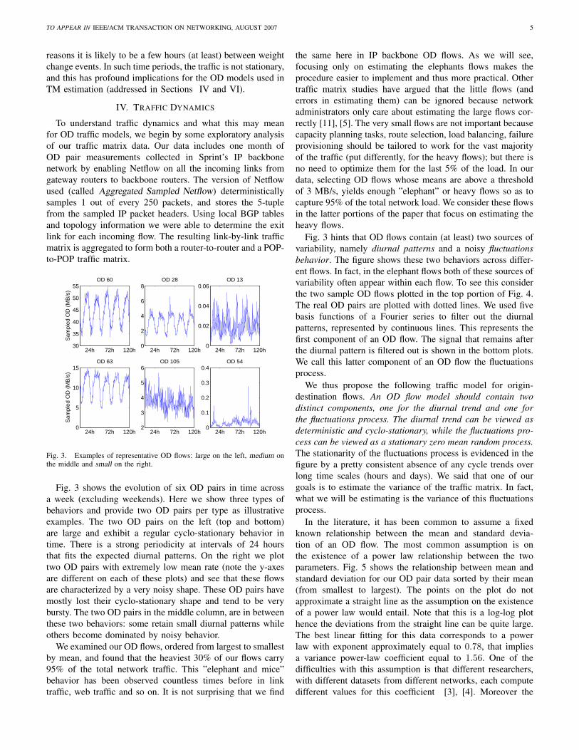
Fig. 3. Examples of representative OD flows: large on the left, medium onthe middle and small on the right.

Fig. 3 shows the evolution of six OD pairs in time acrossa week (excluding weekends). Here we show three types ofbehaviors and provide two OD pairs per type as illustrativeexamples. The two OD pairs on the left (top and bottom)are large and exhibit a regular cyclo-stationary behavior intime. There is a strong periodicity at intervals of 24 hoursthat fits the expected diurnal patterns. On the right we plottwo OD pairs with extremely low mean rate (note the y-axesare different on each of these plots) and see that these flowsare characterized by a very noisy shape. These OD pairs havemostly lost their cyclo-stationary shape and tend to be verybursty. The two OD pairs in the middle column, are in betweenthese two behaviors: some retain small diurnal patterns whileothers become dominated by noisy behavior.

We examined our OD flows, ordered from largest to smallestby mean, and found that the heaviest 30% of our flows carry95% of the total network traffic. This ”elephant and mice”behavior has been observed countless times before in linktraffic, web traffic and so on. It is not surprising that we find

the same here in IP backbone OD flows. As we will see,focusing only on estimating the elephants flows makes theprocedure easier to implement and thus more practical. Othertraffic matrix studies have argued that the little flows (anderrors in estimating them) can be ignored because networkadministrators only care about estimating the large flows cor-rectly [11], [5]. The very small flows are not important becausecapacity planning tasks, route selection, load balancing, failureprovisioning should be tailored to work for the vast majorityof the traffic (put differently, for the heavy flows); but there isno need to optimize them for the last 5% of the load. In ourdata, selecting OD flows whose means are above a thresholdof 3 MB/s, yields enough ”elephant” or heavy flows so as tocapture 95% of the total network load. We consider these flowsin the latter portions of the paper that focus on estimating theheavy flows.

Fig. 3 hints that OD flows contain (at least) two sources ofvariability, namely diurnal patterns and a noisy fluctuationsbehavior. The figure shows these two behaviors across differ-ent flows. In fact, in the elephant flows both of these sources ofvariability often appear within each flow. To see this considerthe two sample OD flows plotted in the top portion of Fig. 4.The real OD pairs are plotted with dotted lines. We used fivebasis functions of a Fourier series to filter out the diurnalpatterns, represented by continuous lines. This represents thefirst component of an OD flow. The signal that remains afterthe diurnal pattern is filtered out is shown in the bottom plots.We call this latter component of an OD flow the fluctuationsprocess.

We thus propose the following traffic model for origin-destination flows. An OD flow model should contain twodistinct components, one for the diurnal trend and one forthe fluctuations process. The diurnal trend can be viewed asdeterministic and cyclo-stationary, while the fluctuations pro-cess can be viewed as a stationary zero mean random process.The stationarity of the fluctuations process is evidenced in thefigure by a pretty consistent absence of any cycle trends overlong time scales (hours and days). We said that one of ourgoals is to estimate the variance of the traffic matrix. In fact,what we will be estimating is the variance of this fluctuationsprocess.

In the literature, it has been common to assume a fixedknown relationship between the mean and standard devia-tion of an OD flow. The most common assumption is onthe existence of a power law relationship between the twoparameters. Fig. 5 shows the relationship between mean andstandard deviation for our OD pair data sorted by their mean(from smallest to largest). The points on the plot do notapproximate a straight line as the assumption on the existenceof a power law would entail. Note that this is a log-log plothence the deviations from the straight line can be quite large.The best linear fitting for this data corresponds to a powerlaw with exponent approximately equal to 0.78, that impliesa variance power-law coefficient equal to 1.56. One of thedifficulties with this assumption is that different researchers,with different datasets from different networks, each computedifferent values for this coefficient [3], [4]. Moreover the

TO APPEAR IN IEEE/ACM TRANSACTION ON NETWORKING, AUGUST 2007 6

24h 72h 120h30

35

40

45

50

55S

ampl

ed O

D (

MB

/s)

24h 72h 120h1

2

3

4

5

6

7OD pair 28

24h 72h 120h−6

−4

−2

0

2

4

6

8

Flu

ctua

tion

Pro

cess

(M

B/s

)

24h 72h 120h−2

−1

0

1

2

3

OD pair 60

Fig. 4. Top: two example real large OD pairs (dotted lines) and their diurnalpatterns (continuous lines). Bottom: the fluctuation process for the two ODpairs obtained by removing the diurnal trends from the original signals.

10−6

10−4

10−2

100

10−6

10−5

10−4

10−3

10−2

10−1

100

101

95% oftraffic

Std

of O

D (

MB

/s)

Mean of OD (MB/s)

Fig. 5. Standard deviation of traffic fluctuations vs the mean traffic volumesfor all the OD pairs (in Mbytes/s).

coefficient varies per OD pair [4]. It is unclear how estimationerrors are impacted by methods relying on this assumption.

In our work, we need not make any such assumption.Instead we remove the power law assumption and choose toestimate the variance directly, and do so independently ofthe mean. Being able to estimate the covariance of the TMhas significant consequences: (1) we avoid having to makequestionable assumptions about the relationship between themean and variance; and (2) we can use our estimate to definea method for identifying the elephants flows. To see this,note that what Fig. 5 does confirm is the hypothesis that ODflows with large variance are also the ones with large mean.Hence there is an implication that the order of magnitudeof the standard deviation is closely related to the order ofmagnitude of the mean for an OD flow. We will make use ofthis observation to help identify the top flows.

V. METHODOLOGY

Our composite methodology makes use of three new ideas:route changes, cyclo-stationary models and variance estimates.

Before describing the details of our models and estimationprocedures, we give here an overall summary of how theseideas are combined to build a composite methodology andsome variants of it. In this paper we essentially proposetwo solutions, termed Algorithm 1 and 2, plus a variant ofAlgorithm 1. Algorithm 1 (below) can be used when one wantsto estimate all the OD flows, while Algorithm 2 can be usedif the one wants only to estimate the elephant OD flows.

Algorithm 1 Estimate all OD flows1. Collect enough SNMP data to estimate the variance ofOD flows.2. Use VRC-heuristic to select minimal set of weightchanges so as to generate full rank system.3. Apply route changes and collect SNMP data from eachsnapshot.4. Expand linear system to include all SNMP data and allrouting configurations. process.5. Use basic inference technique (pseudo-inverse or Gauss-Markov estimators) on full-rank expanded linear system.

We discuss what we mean by ”enough SNMP data” in step1 in Sec. VI-C. If one estimates the OD flow variances,then the Gauss-Markov estimator can be used in Step 5. Avariant of this algorithm can be used if one does not haveenough data to estimate the variances. In that case step 1can be omitted and the pseudo-inverse estimator should beused in Step 5. The advantage of this variant is that it doesnot require any knowledge about traffic fluctuation statistics;however the disadvantage is that it may be less accurate thanthe solution with the variance estimator. In the mathematicaldevelopment of our methods, we also derive a closed formsolution for evaluating the goodness of our variance estimate.This is included herein for completeness, although we do notevaluate it due to lack of space.

A key component in Algorithm 2 is to identify the toplargest OD flows (in advance of estimating their averagevolume). As observed earlier, a weak relation exists betweenthe order or magnitude of the standard deviations and theorder of magnitude of the means. By selecting the flows withthe largest variance, we can be reasonably assured that wehave identified the flows that are largest in mean. We then setthe estimates for the small flows to zero and consider themknown. We thus have fewer variables to estimate as only thelarge flows remain. Having a system with fewer unknowns, wecan run our algorithm for finding the key link weight changesto increase the rank of the system. We expect to need fewersnapshots now since there are fewer variables to estimate.

Comparing the performance of these two solutions willillustrate an important tradeoff. In algorithm 1 we expecthigh estimation accuracy since the system is upgraded tofull rank. However, this may require many snapshots (over20). Algorithm 2 enables a smaller number of snapshotsbut potentially at the expense of accuracy in the estimates.Because the small flows are set to zero, their bandwidth will beredistributed to other flows, thus increasing estimation errors.This tradeoff is quantified in Section VII.

TO APPEAR IN IEEE/ACM TRANSACTION ON NETWORKING, AUGUST 2007 7

Algorithm 2 Estimate heavy (elephant) OD flows1. Collect enough SNMP data to estimate the variance ofOD flows.2. Identify heavy flows. Use threshold policy (definedbelow) to select all OD flows whose variance is abovethreshold. Call the set XL. Reduce linear system by settingto zero all non-elephant flows.3. Use VRC-heuristic to select minimal set of weightchanges so as to make reduced system full rank.4. Apply route changes and collect SNMP data from eachsnapshot.5. Expand linear system to include all SNMP data and allrouting configurations.6. Use basic inference techniques (pseudo-inverse or Gauss-Markov estimators) on full-rank modified linear system.

VI. MODELS AND ESTIMATES

Since we have an OD pair model that includes a diurnalpattern and a fluctuations process, to populate the traffic matrixwith mean estimates now corresponds to extracting the maintrend in time (i.e., a time-varying mean) of the OD pairs, whileestimating the variance collapses to estimating the variance ofthe fluctuation process. (The notation introduced throughoutthis section is summarized in Table I at the end of this section.)

A. Incorporating Routing Changes

We now show how to incorporate the different A(k) matri-ces (from different routing configurations) and all the SNMPdata collected under each of the snapshots, into a expanded(block matrix) linear system. Our traffic matrix estimate here isfor the variant of Algorithm 1 without the variance estimates.In order to build our solution step by step, we assume for themoment that {X(k, n)∀k ∈ [0,K−1] and n ∈ [0, Ns−1]} isa realization of a segment of a stationary discrete time randomprocess. We model each OD pair as follows:

X(k, n) = x+W (k, n) ,∀k ∈ [0, K−1] and n ∈ [0, Ns−1],(2)

where x is a deterministic column vector representing themean of the OD pair, while {W (k, n)} are zero mean columnvectors, i.e. E[W (k, n)] = 0, representing the “traffic fluctu-ation” for the OD pairs at discrete time n in the measurementinterval k. We define Wp(k, n) as the pth component ofW (k, n). Recall that the equation relating the OD traffic flows,routing, and link counts is as follows:

Y (k, n) = A(k)X(k, n) , ∀k ∈ [0,K−1] and n ∈ [0, Ns−1].(3)

To incorporate all the SNMP samples from all of thesnapshots, we build our expanded system by defining thefollowing matrices, using block matrix notation.

Y =

26666664Y (0, 0)

...Y (0, Ns − 1)

...Y (K − 1, Ns − 1)

37777775 , A =

26666664A(0)

...A(0)

...A(K − 1)

37777775

W =

26666664W (0, 0)

...W (0, Ns)

...W (K − 1, Ns − 1)

37777775 , C =

26664A(0) 0 . . . 0

0 A(0) . . . 0...

.... . .

...0 0 . . . A(K − 1)

37775In the new A matrix, each A(k) matrix is repeated Ns

times (for each SNMP sample), since the routing is assumedto stay the same within the same measurement interval k. Wedefine Mk to be rank of matrix Ak. In terms of dimensions,Y is a LNsK-dimensional column vector, A is a LNsK ×P dimensional matrix, W is a KNsP -dimensional columnvector, and C is a LNsK × KNsP matrix. Putting (3) intomatrix form, using (2), we obtain

Y = Ax + CW. (4)

Our aim is to estimate x, denoted x, from the observationsY (0, 0), . . . , Y (0, Ns−1), . . . , Y (K−1, Ns−1). Throughoutthe remainder of the paper, we assume the VRC-heuristic issuccessful and that A is of full rank. One possible approachfor synthesizing our estimate x is to minimize the Euclideannorm of Y −Az, i.e.

x = arg minz{(Y −Az)T (Y −Az)} (5)

=(AT A

)−1AT Y . (6)

This is the Pseudo-Inverse estimator, and does not requireknowledge of the statistics of the traffic fluctuations W .

B. Incorporating Variance Estimates

We point out that the components of the link measurementvector Y will have different variances, due to the varyingnumber of OD pairs traversing each link and the differencesin the variance of the traffic fluctuations of individual ODpairs. Intuitively, a component of the link measurement vectorshould be weighted more heavily if it’s variance is smaller.We were thus motivated to try to improve the above estimateby estimating (next subsection) and incorporating (this sub-section) these variances. We now derive our estimate for thetraffic matrix when the variances are known (for Algorithm1). Let B be the covariance matrix of W , i.e.

B = E[WWT ] . (7)

Let t denote the discrete time across all the measurementintervals, from 0 to T − 1 where T = (KNs) is the totalnumber of samples collected across the whole experiment.There exists a bijective relationship between the discrete timeindex t and the pairs of temporal indexes k and n, i.e.t = kNs + n, where k = bt/Nsc and n = t − bt/NscNs.Then the covariance matrix B can be written as:

B =

R(0) R(1) . . . R(T − 1)R(1) R(0) . . . R(T − 2)

......

. . ....

R(T − 1) R(T − 2) . . . R(0)

, (8)

where R(t) is the P × P matrix defined by:

R(t) = [rp(t)] = diag(E[Wp(τ)Wp(τ + t)]). (9)

TO APPEAR IN IEEE/ACM TRANSACTION ON NETWORKING, AUGUST 2007 8

We assume in (9) that the traffic fluctuations across OD-pairsare uncorrelated, i.e. E[Wp(τ)Wp′(τ + t)] = 0 if p 6= p′.

With this definition, the covariance matrix of Y is equal toCBCT . Assuming (for now) that B is known, the best linearestimate of x given Y , in the sense of minimizing E[(Y −Az)T (Y −Az)] with respect to z is known as the best linearMinimum Mean Square Error (MMSE) estimator. The bestlinear MMSE estimate of x can be obtained from the Gauss-Markov Theorem [12], and is stated as:

x = x(Y, B) =(AT (CBCT )−1A

)−1AT (CBCT )−1Y .

(10)Note that the estimate x in (10) reduces to the pseudo-

inverse estimate when CBCT is the identity matrix. If W hasa Gaussian distribution, it can be verified that the estimate in(10) is in fact the maximum likelihood estimate of x. Thisestimate has the following nice property:

Corollary 3: Regardless of whether or not W is Gaussian,the estimate in Proposition 10 is unbiased, i.e. E[x] = x, andfurthermore we have

x(Y, B) = x +(AT (CBCT )−1A

)−1AT (CBCT )−1CW

and E[(x− x)(x− x)T ] =(AT (CBCT )−1A

)−1.

The proof of this is straightforward and can be found in [10].Note that this last equation allows us to estimate the accuracyof our estimate x of x given Y and B. In particular, the pth

element of the diagonal of the matrix E[(x− x)(x− x)T ] isthe mean square error of our estimate of the pth element ofthe traffic matrix.

C. Estimating the Covariance of Traffic Fluctuations

We now present a method for obtaining an estimate ofthe covariance function of the fluctuations process {W}. Wehighlight two nice characteristics of our method. First, it doesnot require any knowledge of the first order moment statistics.Previous approaches assumed to know exactly the mean torecover the covariance and vice-versa. As a consequence,our method does not suffer from potential error propagationproblems introduced by the first order moment estimation.Second, the estimate does not require any routing configurationchanges. Instead, it relies on a large number of measurementsof the link counts under the same routing configuration.

We define the link correlation matrix as CY (t) =E[Y (τ)Y T (τ + t)]. For two links l and m, each entry of thismatrix is given by:

E

P∑

i=1

P∑

j=1

Al,i[Xi + Wi(τ)]Am,j [Xj + Wj(τ + t)]

=P∑

i=1

Al,iAm,iri(t) +P∑

i=1,j=1,j 6=i

Al,iAm,jE[Xi]E[Xj ].

In the previous statement we assumed that each OD pair isindependent. By using a matrix notation, we can thus write:

CY (t) = AR(t)AT + E[AX]E[AX]T

= AR(t)AT + E[Y (τ)]E[Y (τ + t)]T . (11)

The link covariance matrix is thus given by CY (t) −E[Y (τ)]E[Y (τ + t)]T . This can be estimated directly fromthe sequence of link measurements contained in the linkmeasurement vector Y . Once the link covariance matrix isknown, we can estimate R(t) as follows:

R(t) = arg minZ||CY (t)−AZAT −E[Y (τ)]E[Y (τ + t)]T ||22.

Notice that we can re-write Eqn (11) as γy(t) =Γr(t), where γy(t) is the link covariance matrix, CY (t) −E[Y (τ)]E[Y (τ + t)]T , ordered as a L2-dimensional columnvector, Γ is a L2 × P matrix whose rows are the component-wise products of each possible pair of rows from A, and r(t)is a P -dimensional column vector whose elements are rp(t).With this formulation, an estimate of r(t) can be obtainedusing the pseudo-inverse matrix approach:

r(t) = (ΓT Γ)−1ΓT γy(t). (12)

Our estimate of the variance of the fluctuations process foreach OD-pair is given by the components of r(0). Using astandard estimate for the link covariance matrix, we obtain:

r(0) =1T

T−1∑τ=0

(ΓT Γ)−1ΓT γy(τ) (13)

where the components of γy(τ) are yl(τ)ym(τ)− ylym, andfor each link l we define

yl =1T

T−1∑τ=0

yl(τ) .

To examine the accuracy of the estimate for r(t), we canderive the following after some algebraic manipulations.

E[(r(t)− r(t))T (r(t)− r(t))

]≤

1T 2||Φ||

T−1∑

i=0

L∑

l=1

L∑m=1

E

[y2

l (i)y2m(i + t)− (

E[yl(i)ym(i + t)])2

]

(14)

where Φ = [(ΓT Γ)−1ΓT ]T [(ΓT Γ)−1ΓT ], and ||Φ|| is thenorm (i.e. determinant) of Φ . Equation (14) can be usedto relate the confidence on the r(t) estimate to the fourthorder moments of link-count statistics, which can be evaluatedthrough standard statistical techniques.

D. Incorporating Cyclo-Stationarity

Next, we present out cyclo-stationary model for trafficmatrices and explain its impact on the associated estimationproblem. We now forgo our previous assumption that {X(t)}is a random process with constant mean as in Eqn (2). Insteadwe define our OD flow traffic with

X(t) = x(t) + W (t) , ∀t ∈ [0, T − 1]. (15)

where {X(t)} is cyclo-stationary with period N - in thesense that X(t) and X(t + N) have the same marginaldistribution. More specifically, we assume that {x(t)} is adeterministic (vector valued) sequence, periodic with periodN , and that {W (t)} is a zero-mean stationary random process.

TO APPEAR IN IEEE/ACM TRANSACTION ON NETWORKING, AUGUST 2007 9

In this framework, estimating the traffic matrix now corre-sponds to estimating x(t) for all t given the observations Y (t),0 ≤ t < T = KNs.

We shall assume that x(t) can be represented as theweighted sum of 2Nb + 1 given basis functions, i.e.

x(t) =2Nb∑

h=0

θhbh(t) (16)

where for each h, θh is a P ×1 vector (of “coefficients”), andbh(·) is a scalar “basis” function that is periodic with periodN . In particular, we will consider a Fourier expansion where

bh(t) ={

cos(2πth/N) , if 0 ≤ h ≤ Nb

sin(2πt(h−Nb)/N) , if Nb + 1 ≤ h ≤ 2Nb

(17)Substitution of (16) into (15), and then (3), we obtain

Y (t) = A(k)(2Nb∑

h=0

θhbh(t)) + A(k)W (t)

= A′(t)θ + A(k)W (t),

where we define the (2Nb + 1)P × 1 vector θ according to

θ =

θ0

θ1

...θ2Nb

, (18)

and A′(t) is the L× (2Nb + 1)P matrix defined as

A′(t) =[

A(k)b0(t) A(k)b1(t) · · · A(k)b2Nb(t)

].

(19)Next we re-define the matrix A to be of dimension LT ×

(2Nb + 1)P as follows:

A =

A′(0)A′(1)

...A′(T − 1)

. (20)

The matrices C and W are defined as before. With thisnotation we have an equation similar to equation (4), namely

Y = Aθ + CW . (21)

Thus, we can use the same estimate, from Eqn (10) as before,(or from Eqn (6)) to estimate θ when the covariance B isknown (unknown), respectively. Then we estimate x(t) foreach instant t using Eqn (16) . Our covariance matrix estimatorin Section VI-C can still be used to obtain the covariances inthe system described by Eqn (21). Our estimates for cyclo-stationary OD flows can be applied to the entire traffic matrix(Algorithm 1) or just the elephant flows (Algorithm 2).

E. Identifiability of Second Order Moment

In this section we prove that is always possible to estimatethe covariance function without requiring any routing config-uration changes for any topology.

Theorem 4: For a general connected topology the rank ofΓ is P under any minimum cost routing in which link costsare strictly positive.

Proof: We will prove the theorem by contradiction. If therank of Γ is smaller than P then ker Γ 6= 0, 3 i.e., there existsa non null vector Vo ∈ RP such that ΓV0 = 0. Let T ≤ P bethe number of non null components of V0. Let V be the vectorspace of dimension T generated by all the vectors which havenull components in correspondence to null components of V0.

We consider the correspondence F : V → RT which mapsany vector V ∈ V into a vector W ∈ RT by discardingnull components of V . Let Γ be the matrix obtained by Γby discarding the columns that in the multiplication ΓV withV ∈ V would not contribute (since multiplied by null elementsof V ). By construction ΓV = ΓW for any V ∈ V . Finally letW0 the vector which corresponds to V0 though F . We noticethat every component of W0 is not null.

Let us consider the set Zod of OD pairs which correspondto the elements of W0. We will show that there exists at least apair of links in the network which are jointly crossed by justone OD pair in Zod. Thus the row of Γ which correspondsto the considered pair of links must contain only one elementdifferent from 0 . As a consequence, necessarily, it results thatΓW0 6= 0, in contradiction with the previous assumptions.

Indeed, let us compute path-cost (sum of the link weights)for any OD pair in Zod. Let zod be an OD pair in Zod whichcorresponds to a maximum path cost. Consider the first andthe last link (l and m respectively) spanned by the zod path.

We claim that zod is the only OD pair in Zod which crossesboth links l and m. By construction zod crosses both l and m.In addition we show by contradiction that no other OD pairscan cross l and m. Assume z′od 6= zod crosses both links l andm then there are only two possibilities: 1) l is the first andm the last link of the z′od path; in this case however both theorigin and the destination of z′od would be coincident with theorigin and the destination of zod then contradicting the factthat z′od 6= zod; 2) either l is not the first link or m is not thelast link of the path spanned by z′od; in this case however thepath cost of z′od is larger than the path cost of zod (since thesub-path of z′od from l to m necessarily has the same cost ofthe whole zod path) thus contradicting the fact that the pathcost of zod is maximum.

VII. RESULTS

We now evaluate our two algorithms using the trafficmatrix data from Sprint’s commercial Tier-1 backbone. In bothsolutions, we used a pseudo-inverse estimator as our basicinference method in the last step. We used this, rather thanthe Gauss-Markov estimator because (as explained later), wedid not have enough months of Netflow data to do a propercomparison using Gauss-Markov estimators.

1) Evaluation of Algorithm 1: Estimating the Whole TrafficMatrix: We now assess the accuracy of the mean estimationwhen the traffic matrix is computed using Algorithm 1. Forour network scenario considered, the VRC-heuristic algorithm

3We recall that, given a linear operator Γ, ker Γ denotes the set of vectorswhose image through Γ is 0, i.e., v ∈ ker Γ iff Γv = 0.

TO APPEAR IN IEEE/ACM TRANSACTION ON NETWORKING, AUGUST 2007 10

Notation DefinitionL, l number of network links, link indexP , p number of OD pairs, OD pair indexK, k number of measurement intervals (i.e., snapshots),

snapshot indexNs number of SNMP samples collected in a snapshotYl(k, n) traffic volume (bytes) on link l during measurement

interval k at discrete time nY (k, n) link count vectorXp(k, n) traffic volume of OD pair p during measurement

interval k at time nX(k, n) traffic matrix organized as a vector at time n

during snapshot kA(k) routing matrix during snapshot kA block form of routing matrix including A(k) ∀kWp(k, n) fluctuation/noise process for OD pair p at

time n in snapshot kW (k, n) noise column vectort time index, t = kNs + nC block-form routing matrix relating OD fluctuations

to link countsB covariance matrix of noise Wrp(t) autocorrelation of OD pair p over time lag tr(t) vector of OD pair autocorrelations.

r(0) is vector of OD variancesR(t) matrix form with r(t) on diagonal & 0’s elsewhereCY (t) link correlation matrixγy(t) link covariance matrix ordered as a column vectorΓ matrix whose rows are component-wise products of

all pairs of rows of Abh(·),θh basis function & coefficient of Fourier expansionNb number of basis functions in cyclo-stationary model

TABLE IGLOSSARY OF NOTATION

determined that K = 24 snapshots were sufficient to identifyall the OD pairs. Of these 24 snapshots, 22 of them involveonly one link weight change at a time, while the last twoinvolve two simultaneous link weight changes.

For illustrative purposes, we first look at our estimates overtime for six particular OD pairs (see Fig. 6). For each flow,these graphs show the temporal shapes of the real, de-noised,and estimated OD pair. The de-noised OD pair refers to anOD pair with everything filtered out except the first 5 basisfunctions of Fourier series; put alternatively, this illustrateshow well a simple Fourier model captures the changing meanbehavior. Our model fits these flows extremely well. It isinteresting that the quality of the estimation obtained decreasesas the average rate drops. The two on the right do sufferfrom larger errors. Note that these two OD flows (#28 and#105) were the worst case performing OD flow estimates fromwithin the heavy flow category. Our method exhibits the samebehavior as other methods in that it estimates large flows welland has difficulty as the flows get smaller and smaller.

The gain of our method comes in terms of the actualestimation errors achieved for these top flows. To examineestimation errors in general, we use the following two metrics.First, we examine the difference between the first componentof the Fourier series, i.e. the continuous component, for theNetflow data and the estimation provided by our models. Since

8h 16h 24h60

70

80

90

100

110

Sam

pled

OD

(M

B/s

)

8h 16h 24h5

10

15

20

25OD 56

8h 16h 24h0

5

10

15OD 28

8h 16h 24h10

15

20

25

30OD 63

Sam

pled

OD

(M

B/s

)

8h 16h 24h0

10

20

30OD 39

8h 16h 24h0

5

10

15OD 105

OD 60

Fig. 6. Method 1. Mean Estimation. Real OD flow (continuous line), de-noised OD flow (dotted line), and estimated OD flow (dashed line).

this part of our estimate would be used to populate a trafficmatrix, we compute the relative error of this estimate. Second,since we have a temporal process, we need to examine theerrors in estimation over time. We thus use the difference inenergy between the estimate Xp(t) and the real data Xp(t).In particular, we use the relative L2-norm to estimate thegoodness of the model fitting, ||Xp(t)− Xp(t)||22/||Xp(t)||22.

Fig. 7 shows our first metric on the difference of the firstcomponent of the Fourier series for the real data (x-axis) andthe estimated OD pairs (y-axis) for the elephant flows whenNs = 100 samples per snapshot are used. The average error is3.8%. This is a large improvement over other methods whoseaverage errors typically lie somewhere between 11%-23%. 4

Some carriers have indicated that they would not use trafficmatrices for traffic engineering unless the inference methodscould drive the average errors below the 10% barrier. Webelieve that this is the first study to achieve this.

Among these flows, the worst case relative error across allOD pairs is 28%. If we look carefully at the figure, we cansee that all the flows have less than 10% relative error, exceptfor four outliers. These outliers correspond to OD pairs whoseaverage rate is less than 5 MB/s, i.e. among the smallest ODflows within the “heavy” ones represented here. For 90% ofthese top flows (i.e., excluding these four outliers), the averageerror drops below 2% and the worst case relative error dropsto 4.6%. (See the first column in Table II for 24 snapshots.)We remind the reader that small OD pairs (those whose rate isunder 3 MB/s) do not appear in the figure but are consideredin the system and are thus a part of the overall computation.

Fig. 8 shows the L2-norm relative error cumulatively. Inmost of our calculations the number of basis functions weused was Nb = 5 and the number of samples per snapshotused was Ns = 100. This figure shows that the worst case

4It is hard to compare numbers exactly because different studies usedifferent amounts of total load. However we capture more total traffic thanmost other studies that typically include 75% or 80% of the network-wideload.

TO APPEAR IN IEEE/ACM TRANSACTION ON NETWORKING, AUGUST 2007 11

2 4 6 8 10 12 14 16 18 20

2

4

6

8

10

12

14

16

18

20

10%

Real mean of OD (MB/s)

Est

imat

ed m

ean

of O

D (

MB

/s)

Fig. 7. Method 1. Relative error of 1st component of Fourierseries for top flows with Ns = 100.

10−2

100

102

0

0.1

0.2

0.3

0.4

0.5

0.6

0.7

0.8

0.9

1

Relative L2−norm error across a day

Cum

mul

ativ

e nu

mbe

r of

OD

pai

rs

Nb=3, Ns=10Nb=3, Ns=100Nb=5, Ns=10Nb=5, Ns=100

Fig. 8. Method 2. Cumulative distribution of the relative L2-normerror for top flows as a function of Nb and Ns.

L2-norm relative error was 56% corresponding to OD pair#28 (the second worst case is 44%, corresponding to OD pair#105). We see that 85% of the flows had an L2-norm errorof less than 10% (see OD pairs #56 and #39 as an example).Fig. 6 helps us understand the effects of the L2-norm error.As we can see our model captures the diurnal trends correctlyfor the heavy OD pairs, but can suffer with relatively “small”OD flows.

We highlight the difference between our two error metrics.Others have reported relative errors on their mean estimateswhere the means are computed over some specific interval(often fairly long). Our L2-norm relative error is an error rateon our estimation (or fitting) of the dynamic OD flow varyingin time; put alternatively it summarizes “instantaneous” errorsin OD flow modeling. We cannot compare the value of thislatter metric to other studies because they have not tried tobuild a model capturing the temporal behavior.

The performance of our method is influenced by the numberof samples per snapshot and the number of basis functionsused (see Fig. 8. Intuitively, a larger number of basis functionNb will lead to a better quality estimate, although at the costof a larger number of samples. The number of samples Ns

plays an important role independently of the number of basisfunctions implemented. The more samples collected, the moreis learned about the temporal evolution of each OD pair, anda better estimation can be provided. For a fixed number ofbasis functions, going from Ns = 10 to Ns = 100 yields asubstantial improvement. In our experimentation, using morethan 5 basis functions yielded insignificant gains and thus wedecided to set Nb = 5 for the remainder of our evaluation.

2) Evaluation of Algorithm 2: Estimating Elephant ODPairs Only : We start by estimating the variance (Step 1) ofthe OD flows using Eqn (13). For Step 2, we order the ODflows by size of variance. By relying upon our observationthat flows that have large variance are also typically large inmean, the task now is to set a threshold and select the “heavy”flows above this threshold. Two issues arise when doing this.

As discussed in Section VI, the nice feature about ourvariance estimator is that it does not require any routingchanges. However a large number of SNMP samples arerequired to force the relative error of the variance estimate

to be under 5%. We selected the 5% target arbitrarily. Aftersome experimentation we found that roughly 25,000 sampleswere needed to achieve this target level of accuracy. In areal network this implies one needs about 3 months worthof SNMP data. In commercial networks obtaining this muchhistorical data is not a problem as all ISPs store their SNMPdata for multi-year periods. Although we had plenty of months(years) of SNMP data, we did not have 3 months of Netflowdata available to us that would have been needed to do acomplete validation of this method.

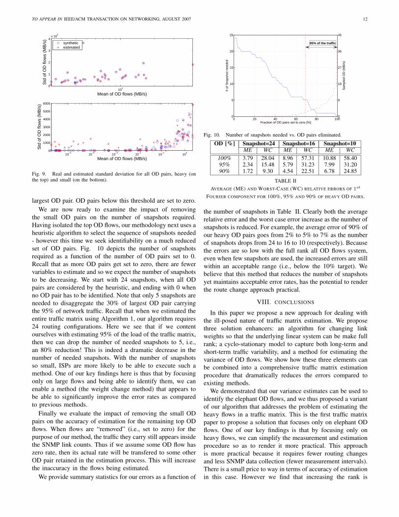
We therefore decided to use pseudo-real data for this evalua-tion. We call this pseudo-real data because it is generated basedon a model fitted to actual data (but only one month’s worth).To create sample OD flows, we filter out the noise from each ofour sampled OD pairs and keep only the first five componentsof the matched Fourier series. We generate sample OD flows,over longer periods of time, using this Fourier series model towhich we add a zero mean gaussian noise with a power-lawvariance whose coefficient is set to 1.56 (in accordance withthe empirical data observed in Fig. 5). We route this traffic(according to the original A matrix, i.e. snapshot k = 0) andgenerate what would be the resulting SNMP link counts forthe 3 month period under study. This last step is the same asthe methodology presented in [6].

We compare our estimate of the standard deviation (std) tothe standard deviation of the pseudo-real data in Fig. 9. The topplot is for the elephant flows, while the bottom plot includesthe comparison for small flows. The variance estimate for themedium and large OD flows is quite good in that it achievesan average estimation error of less than 5%. As expected, it isharder to estimate the variance of the smaller OD pairs and wesee the errors can span a large range. This challenge cannot bemet by merely increasing the number of samples because it isdue to the difference in order of magnitude of large and smallOD pairs. As a consequence, a small error in the std-estimateof large OD pairs will be spread across multiple OD pairscausing large errors in the std-estimate of small OD pairs.

Without a method for extracting exactly the top 30% largestOD pairs from the rest, we rely on a simple threshold schemefor now. We keep all OD pairs whose rates are above athreshold set to be two orders of magnitude lower than the

TO APPEAR IN IEEE/ACM TRANSACTION ON NETWORKING, AUGUST 2007 12

101

0

1

2

3

4x 10

4

Std

of O

D fl

ows

(MB

/s)

Mean of OD flows (MB/s)

syntheticestimated

10−5

10−4

10−3

10−2

10−1

100

0

1000

2000

3000

4000

5000

6000

Std

of O

D fl

ows

(MB

/s)

Mean of OD flows (MB/s)

Fig. 9. Real and estimated standard deviation for all OD pairs, heavy (onthe top) and small (on the bottom).

largest OD pair. OD pairs below this threshold are set to zero.We are now ready to examine the impact of removing

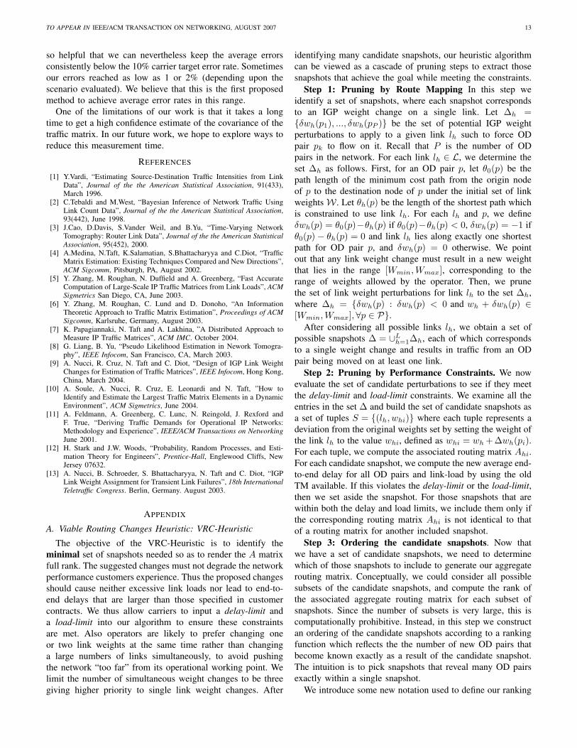
the small OD pairs on the number of snapshots required.Having isolated the top OD flows, our methodology next uses aheuristic algorithm to select the sequence of snapshots needed- however this time we seek identifiability on a much reducedset of OD pairs. Fig. 10 depicts the number of snapshotsrequired as a function of the number of OD pairs set to 0.Recall that as more OD pairs get set to zero, there are fewervariables to estimate and so we expect the number of snapshotsto be decreasing. We start with 24 snapshots, when all ODpairs are considered by the heuristic, and ending with 0 whenno OD pair has to be identified. Note that only 5 snapshots areneeded to disaggregate the 30% of largest OD pair carryingthe 95% of network traffic. Recall that when we estimated theentire traffic matrix using Algorithm 1, our algorithm requires24 routing configurations. Here we see that if we contentourselves with estimating 95% of the load of the traffic matrix,then we can drop the number of needed snapshots to 5, i.e.,an 80% reduction! This is indeed a dramatic decrease in thenumber of needed snapshots. With the number of snapshotsso small, ISPs are more likely to be able to execute such amethod. One of our key findings here is thus that by focusingonly on large flows and being able to identify them, we canenable a method (the weight change method) that appears tobe able to significantly improve the error rates as comparedto previous methods.

Finally we evaluate the impact of removing the small ODpairs on the accuracy of estimation for the remaining top ODflows. When flows are “removed” (i.e., set to zero) for thepurpose of our method, the traffic they carry still appears insidethe SNMP link counts. Thus if we assume some OD flow haszero rate, then its actual rate will be transfered to some otherOD pair retained in the estimation process. This will increasethe inaccuracy in the flows being estimated.

We provide summary statistics for our errors as a function of

0 20 40 60 80 1000

5

10

15

20

25

# of

Sna

psho

t nee

ded

Fraction of OD pairs set to zero [%]

0

9

18

27

36

45

95% of the traffic

Sam

pled

OD

(M

B/s

)

Fig. 10. Number of snapshots needed vs. OD pairs eliminated.

OD [%] Snapshot=24 Snapshot=16 Snapshot=10ME WC ME WC ME WC

100% 3.79 28.04 8.96 57.31 10.88 58.4095% 2.34 15.48 5.79 31.23 7.99 31.2090% 1.72 9.30 4.54 22.51 6.78 24.85

TABLE IIAVERAGE (ME) AND WORST-CASE (WC) RELATIVE ERRORS OF 1st

FOURIER COMPONENT FOR 100%, 95% AND 90% OF HEAVY OD PAIRS.

the number of snapshots in Table II. Clearly both the averagerelative error and the worst case error increase as the number ofsnapshots is reduced. For example, the average error of 90% ofour heavy OD pairs goes from 2% to 5% to 7% as the numberof snapshots drops from 24 to 16 to 10 (respectively). Becausethe errors are so low with the full rank all OD flows system,even when few snapshots are used, the increased errors are stillwithin an acceptable range (i.e., below the 10% target). Webelieve that this method that reduces the number of snapshotsyet maintains acceptable error rates, has the potential to renderthe route change approach practical.

VIII. CONCLUSIONS

In this paper we propose a new approach for dealing withthe ill-posed nature of traffic matrix estimation. We proposethree solution enhancers: an algorithm for changing linkweights so that the underlying linear system can be make fullrank; a cyclo-stationary model to capture both long-term andshort-term traffic variability, and a method for estimating thevariance of OD flows. We show how these three elements canbe combined into a comprehensive traffic matrix estimationprocedure that dramatically reduces the errors compared toexisting methods.

We demonstrated that our variance estimates can be used toidentify the elephant OD flows, and we thus proposed a variantof our algorithm that addresses the problem of estimating theheavy flows in a traffic matrix. This is the first traffic matrixpaper to propose a solution that focuses only on elephant ODflows. One of our key findings is that by focusing only onheavy flows, we can simplify the measurement and estimationprocedure so as to render it more practical. This approachis more practical because it requires fewer routing changesand less SNMP data collection (fewer measurement intervals).There is a small price to way in terms of accuracy of estimationin this case. However we find that increasing the rank is

TO APPEAR IN IEEE/ACM TRANSACTION ON NETWORKING, AUGUST 2007 13

so helpful that we can nevertheless keep the average errorsconsistently below the 10% carrier target error rate. Sometimesour errors reached as low as 1 or 2% (depending upon thescenario evaluated). We believe that this is the first proposedmethod to achieve average error rates in this range.

One of the limitations of our work is that it takes a longtime to get a high confidence estimate of the covariance of thetraffic matrix. In our future work, we hope to explore ways toreduce this measurement time.

REFERENCES

[1] Y.Vardi, “Estimating Source-Destination Traffic Intensities from LinkData”, Journal of the the American Statistical Association, 91(433),March 1996.

[2] C.Tebaldi and M.West, “Bayesian Inference of Network Traffic UsingLink Count Data”, Journal of the the American Statistical Association,93(442), June 1998.

[3] J.Cao, D.Davis, S.Vander Weil, and B.Yu, “Time-Varying NetworkTomography: Router Link Data”, Journal of the the American StatisticalAssociation, 95(452), 2000.

[4] A.Medina, N.Taft, K.Salamatian, S.Bhattacharyya and C.Diot, “TrafficMatrix Estimation: Existing Techniques Compared and New Directions”,ACM Sigcomm, Pitsburgh, PA, August 2002.

[5] Y. Zhang, M. Roughan, N. Duffield and A. Greenberg, “Fast AccurateComputation of Large-Scale IP Traffic Matrices from Link Loads”, ACMSigmetrics San Diego, CA, June 2003.

[6] Y. Zhang, M. Roughan, C. Lund and D. Donoho, “An InformationTheoretic Approach to Traffic Matrix Estimation”, Proceedings of ACMSigcomm, Karlsruhe, Germany, August 2003.

[7] K. Papagiannaki, N. Taft and A. Lakhina, ”A Distributed Approach toMeasure IP Traffic Matrices”, ACM IMC. October 2004.

[8] G. Liang, B. Yu, “Pseudo Likelihood Estimation in Nework Tomogra-phy”, IEEE Infocom, San Francisco, CA, March 2003.

[9] A. Nucci, R. Cruz, N. Taft and C. Diot, “Design of IGP Link WeightChanges for Estimation of Traffic Matrices”, IEEE Infocom, Hong Kong,China, March 2004.

[10] A. Soule, A. Nucci, R. Cruz, E. Leonardi and N. Taft, ”How toIdentify and Estimate the Largest Traffic Matrix Elements in a DynamicEnvironment”, ACM Sigmetrics, June 2004.

[11] A. Feldmann, A. Greenberg, C. Lunc, N. Reingold, J. Rexford andF. True, “Deriving Traffic Demands for Operational IP Networks:Methodology and Experience”, IEEE/ACM Transactions on NetworkingJune 2001.

[12] H. Stark and J.W. Woods, “Probability, Random Processes, and Esti-mation Theory for Engineers”, Prentice-Hall, Englewood Cliffs, NewJersey 07632.

[13] A. Nucci, B. Schroeder, S. Bhattacharyya, N. Taft and C. Diot, “IGPLink Weight Assignment for Transient Link Failures”, 18th InternationalTeletraffic Congress. Berlin, Germany. August 2003.

APPENDIX

A. Viable Routing Changes Heuristic: VRC-Heuristic

The objective of the VRC-Heuristic is to identify theminimal set of snapshots needed so as to render the A matrixfull rank. The suggested changes must not degrade the networkperformance customers experience. Thus the proposed changesshould cause neither excessive link loads nor lead to end-to-end delays that are larger than those specified in customercontracts. We thus allow carriers to input a delay-limit anda load-limit into our algorithm to ensure these constraintsare met. Also operators are likely to prefer changing oneor two link weights at the same time rather than changinga large numbers of links simultaneously, to avoid pushingthe network “too far” from its operational working point. Welimit the number of simultaneous weight changes to be threegiving higher priority to single link weight changes. After

identifying many candidate snapshots, our heuristic algorithmcan be viewed as a cascade of pruning steps to extract thosesnapshots that achieve the goal while meeting the constraints.

Step 1: Pruning by Route Mapping In this step weidentify a set of snapshots, where each snapshot correspondsto an IGP weight change on a single link. Let ∆h ={δwh(p1), ..., δwh(pP )} be the set of potential IGP weightperturbations to apply to a given link lh such to force ODpair pk to flow on it. Recall that P is the number of ODpairs in the network. For each link lh ∈ L, we determine theset ∆h as follows. First, for an OD pair p, let θ0(p) be thepath length of the minimum cost path from the origin nodeof p to the destination node of p under the initial set of linkweights W . Let θh(p) be the length of the shortest path whichis constrained to use link lh. For each lh and p, we defineδwh(p) = θ0(p)−θh(p) if θ0(p)−θh(p) < 0, δwh(p) = −1 ifθ0(p)− θh(p) = 0 and link lh lies along exactly one shortestpath for OD pair p, and δwh(p) = 0 otherwise. We pointout that any link weight change must result in a new weightthat lies in the range [Wmin,Wmax], corresponding to therange of weights allowed by the operator. Then, we prunethe set of link weight perturbations for link lh to the set ∆h,where ∆h = {δwh(p) : δwh(p) < 0 and wh + δwh(p) ∈[Wmin,Wmax], ∀p ∈ P}.

After considering all possible links lh, we obtain a set ofpossible snapshots ∆ = ∪L

h=1∆h, each of which correspondsto a single weight change and results in traffic from an ODpair being moved on at least one link.

Step 2: Pruning by Performance Constraints. We nowevaluate the set of candidate perturbations to see if they meetthe delay-limit and load-limit constraints. We examine all theentries in the set ∆ and build the set of candidate snapshots asa set of tuples S = {(lh, whi)} where each tuple represents adeviation from the original weights set by setting the weight ofthe link lh to the value whi, defined as whi = wh +∆wh(pi).For each tuple, we compute the associated routing matrix Ahi.For each candidate snapshot, we compute the new average end-to-end delay for all OD pairs and link-load by using the oldTM available. If this violates the delay-limit or the load-limit,then we set aside the snapshot. For those snapshots that arewithin both the delay and load limits, we include them only ifthe corresponding routing matrix Ahi is not identical to thatof a routing matrix for another included snapshot.

Step 3: Ordering the candidate snapshots. Now thatwe have a set of candidate snapshots, we need to determinewhich of those snapshots to include to generate our aggregaterouting matrix. Conceptually, we could consider all possiblesubsets of the candidate snapshots, and compute the rank ofthe associated aggregate routing matrix for each subset ofsnapshots. Since the number of subsets is very large, this iscomputationally prohibitive. Instead, in this step we constructan ordering of the candidate snapshots according to a rankingfunction which reflects the the number of new OD pairs thatbecome known exactly as a result of the candidate snapshot.The intuition is to pick snapshots that reveal many OD pairsexactly within a single snapshot.

We introduce some new notation used to define our ranking

TO APPEAR IN IEEE/ACM TRANSACTION ON NETWORKING, AUGUST 2007 14

function. Let Γhi be the set of OD pairs whose routing isaffected by changing the link weight on link lh to the newvalue whi = wh + ∆wh(pi). Let βhi(p) be a binary variablethat is equal to 1 if the OD pair p uses the link lh and 0otherwise, with respect to the new set of link weights afterchanging the weight of link lh to whi as described above. LetRhi(pt) be the set of new links along the path used by ODpair pt after applying the IGP weight whi, i.e. the set of linksthat are contained in a shortest path for pt after changing thelink weight wh to whi but are not included in any shortestpath for pt for the original set of weights W . We define theambiguity of pt after the weight change (lh, whi) to be

mhi(pt) = minlh∈Rhi

∑

p∈Γhi/pt

βhi(p) ∀whi : (lh, whi) ∈ S,

(22)which takes the minimum of these per-link sums across allthe new links in the new path of OD pair pt. The quantitymhi(pt) is defined for a single OD pair pt. Our ranking metricfor changing link lh to the value whi, is defined over all ODpairs as follows.

Mhi =∑

pt∈Γhi

(1/(Bmhi(pt) + 1)) ∀whi : (lh, whi) ∈ S,

(23)where B is a large parameter satisfying the constraint P/(B+1) < 1.

In defining the ranking function we have assumed that isbetter to know something exactly than simply to get new linkcounts without any complete disaggregation. The snapshots arethen ranked according to the corresponding value of Mhi foreach snapshot, where the snapshot with the largest value ofMhi is at the top of the list.

Step 4: Evaluation of candidate single link snapshots. Wenow evaluate the candidate snapshots in the order defined inStep 3. Each entry (lh, whi) ∈ S is evaluated sequentially byappending its associated routing matrix Ahi to the improvedaggregate routing matrix A and computing the rank of thecombined routing matrix. Only if the rank of the new Aincreases then Ahi is kept in A; otherwise the snapshot isdiscarded. The algorithm stops when the rank of the A matrixis equal to P .

Step 5: Multiple IGP weight changes and relaxationof requirements. For large networks performing only singleweight changes might not be enough to guarantee that we haveobtain a full rank routing matrix A. If this is the case, thenwe apply snapshots corresponding to weight changes on pairsof adjacent links and repeat the above steps starting from Step1. In this context, a pair of links is defined to be adjacent ifthey are incident to a common node. The process continuesuntil the aggregate routing matrix has full rank. If we exhaustall snapshots corresponding to a pair of link weight changesthen we try snapshots corresponding to triplets of links. Weconsider only triplets of links that form “triangles”, i.e. tripletsof links of the form {(a, b), (b, c), (c, a)}. Moreover for eachtriplet of links we only consider two possible weight changes,i.e. changing the weights of all three links to either Wmin orall to Wmax. The process continues until the aggregate routing

matrix has full rank. If we reach this point and the rank of Ais less than P , then we relax the delay and load constraints.

Augustin Soule received his PhD from the Univer-sity of Pierre et Marie Curie in 2006, and a M. sc.in Electronics Engineering in 2001 from ISEP, inFrance. He is currently a researcher at ThomsomParis Research Lab. His research interests lie inlarge-scale network measurement, traffic modelingand anomaly detection.

Antonio Nucci (M’99-SM’05) received the Dr. IngDegree in Electronics Engineering in 1998 and thePh.D. degree in telecommunications engineering in2002, both from the Politecnico di Torino, Turin,Italy. From 2001-2005 he worked in Sprint’s Ad-vanced Technology Laboratories in the IP researchgroup. He is currently Chief Technology Officer atNarus Inc. His research interests include traffic mea-surement, characterization, analysis and modeling,security and network design.

R. L. Cruz ( F’03) received the B.S. and Ph.D. de-grees in Electrical Engineering from the Universityof Illinois, Urbana, in 1980 and 1987, respectively,and the S.M.E.E. degree from the MassachussettsInstitute of Technology in 1982. Since 1987, Dr.Cruz has been on the faculty at the University ofCalifornia, San Diego.

Emilio Leonardi (M’99) received a Dr.Ing degreein Electronics Engineering in 1991 and a Ph.D.in Telecommunications Engineering in 1995 bothfrom Politecnico di Torino. In 1995, he visited theUCLA Computer Science Dept. In 1999 he joinedthe High Speed Networks Research Group, at BellLabs/Lucent. He is currently an Associate Professorat the Dipartimento di Elettronica of Politecnicodi Torino. His research interests lie in performanceevaluation, queueing theory, packet switching, wire-less networks, and optical networks.

Nina Taft (M’94) is a senior researcher at IntelResearch Berkeley. She received her PhD (1994)and MS (1990) both from UC Berkeley, and herBS from the University of Pennsylvania in 1985.From 1995-1999, she worked at SRI International;and from 1999-2003, she was a member of the IPGroup at Sprint Advanced Technology Labs Herinterests lie in traffic characterization and modeling,performance evaluation, network design and enter-prise network security.