estimating economies of scale and scope with flexible technology

Estimating Economies of Scale and Scope with Flexible Technology

Thomas P. Triebs David S. Saal Pablo Arocena

Subal C. Kumbhakar

Ifo Working Paper No. 142

October 2012

An electronic version of the paper may be downloaded from the Ifo website www.cesifo-group.de.

Ifo Institute – Leibniz Institute for Economic Research at the University of Munich

Ifo Working Paper No. 142

Estimating Economies of Scale and Scope with Flexible Technology

Abstract Economies of scale and scope are typically modelled and estimated using cost functions that are common to all firms in an industry irrespective of whether they specialize in a single output or produce multiple outputs. We suggest an alternative flexible technology model that does not make this assumption and show how it can be estimated using standard parametric functions including the translog. The assumption of common technology is a special case of our model and is testable econometrically. Our application is for publicly owned US electric utilities. In our sample, we find evidence of economies of scale and vertical economies of scope. But the results do not support a common technology for integrated and specialized firms. In particular, our empirical results suggest that restricting the technology might result in biased estimates of economies of scale and scope.

JEL Code: D24, L25, L94, C51.

Keywords: Economies of scale and scope, flexible technology, electric utilities, vertical integration, translog cost function.

Thomas P. Triebs Ifo Institute – Leibniz Institute for

Economic Research at the University of Munich

Poschingerstr. 5 81679 Munich, Germany

Phone: +49(0)89/9224-1258 [email protected]

David S. Saal Aston University Aston Triangle

B$ 7ET Birminghamton, UK


Pablo Arocena

Public University of Navarre Business Administration Department

Campus of Arrosadia 31006 Pamplona, Spain


Subal C. Kumbhakar State University of New York

at Binghamton Department of Economics

PO Box 6000 Binghamton, New York 13902-6000, USA


2

1. Introduction

Economies of scale and scope are fundamental concepts explaining many economic decisions.

From a business perspective, they play a central role in assessing the potential benefits of

firms’ growth and diversification strategies. From an industry perspective, they are central for

the determination of efficient market structures. In particular, they are the basis for the

restructuring and deregulation of network industries worldwide. For instance, changes in the

economies of scale of electricity generation swayed many countries to liberalize electricity

markets. Subsequently the belief that gains from competition would outstrip any losses in

economies of scope led many countries to mandate electric utilities to divest their generation

assets to prevent discrimination in newly developed wholesale markets. Similarly many banks

today argue that economies of scale and scope make large integrated banks more efficient and

caution against their break-up to minimize the risk from individual bank failures.

Duality theory1 allows us to estimate the underlying production technology via a cost

function. Thus almost the entire literature on the estimation of economies of scale and scope

follows the seminal work of Baumol et al. (1982) and employs a cost function based approach,

which allows identification of the “the production technology of the firms in an industry”.

That is, it is (implicitly) assumed that all the firms in an industry share the same production

technology. Hence, empirical studies have traditionally focused on the estimation of an

industry cost function, common to all firms in the industry. However, this approach ignores

the theoretical, but empirically testable possibility that different types of firms employ

different production technologies. Moreover, maintaining the assumption of a common

technology when heterogeneous technologies are present could potentially lead to biased

estimates of costs and therefore, biased estimates of economies of scale and scope.

Our approach therefore departs from the existing modelling approach for measuring

scale and scope economies by allowing for differences in technologies across firms types.

This is accomplished by specifying a model where technology can be fully flexible across

specialized and non-specialized firms. We therefore allow for firm-type specific technologies

which are estimated jointly without separating the sample. We demonstrate that this approach

can be applied to any functional form including the popular translog form introduced by

Christensen et al. (1973). This is important because, despite the widely accepted advantages

of the translog specification, the non-admission of zero values in the translog form has

1 Duality theory and the implied restrictions on the cost function ensure that the latter does not violate the physics of production. For an introduction see the survey by Fuss und McFadden (1978).

3

previously been seen as precluding its use for the estimation of economies of scope (Caves et

al. 1980). Our model is conceptually different from models that try to estimate production

functions involving zero output quantities (Battese, 1997), and it is more general than other

attempts to estimate separate technologies (e.g., Weninger 2003, Bottasso et al. 2011) because

it does not require a Box-Cox transformation which is difficult to estimate. That is, our model

is easier to implement for the applied researcher as it is linear in parameters and all

coefficients have direct economic interpretations (at the mean of the data). We finally note

that our model readily allows for statistical testing of whether a common or flexible firm type

technology specification is appropriate,

We empirically demonstrate the usefulness of our modelling approach by estimating

economies of scale and scope with a sample of publicly-owned US electric companies.

Although our modelling approach is applicable with any functional form, our empirical

specification demonstrates that, contrary to popular belief, a translog specification can be used

to represent the technology for both specialized and non-specialized firms. Our data is

suitable for this task as it comprises both specialized (generating-only and distributing-only)

and integrated firms. Our results indicate that within our sample, cost relationships differ

between integrated and specialized firms, suggesting that the assumption of a restricted

technology may indeed lead to biased estimates of economies of scale and scope in our

sample.

The rest of the paper is organized as follows. Section 2 provides the necessary

theoretical background including the relevant literature. Section 3 sets out our contribution to

the modelling of economies of scale and scope. Section 4 introduces our empirical model and

tests. Section 5 introduces our application. Section 6 presents the results and section 7 gives a

short conclusion.

2. Scale and Scope Economies with a Common Technology

There are a vast number of studies that estimate economies of scale and scope for various

multiproduct industries. We do not review this literature here. Instead we provide a short

summary of the debate on how to model and estimate multiproduct or multistage cost

functions. We first recall the definition of scale and scope economies. Let N = {1,2,…,N} be

the set of products under consideration, with output quantities y = (y1,…,yn). The function

C(y,w) denotes the minimum cost of producing the entire set of products, at the output

4

quantities and input prices indicated by the vectors y and w. The degree of scale economies

defined over the entire product set N, at y, is given by

1 ,,

∑ ,1

∑ ln / ln

where Ci is the first derivative of cost with respect to product i. Returns to scale are said to be

increasing, decreasing or constant as S is greater than, less than, or equal to unity, respectively.

Let us now consider two subsets, SU N, and SD N such that SU SD = N, and SU ∩ SD

= Ø. Let yU denote the vector whose elements are set equal to those of y for i SU and yD

denote the vector whose elements are set equal to those of y for i SD. Similarly, C(yU,w)

and C(yD,w) denote the cost of producing only the products in the subset U and D,

respectively. The degree of economies of scope between yU and yD is defined as

2 , ,, , ,

,

The degree of economies of scope SC is measured by (2) where the separation of

production is said to increase, decrease or leave unchanged the total cost as SC is greater than,

less than, or equal to zero, respectively. Equation (2) shows that the estimation of economies

of scope (i.e. the costs and benefits of joint production) requires the comparison of costs

between specialized and non-specialized firms at a given vector of input prices. In our below

application, this measure of economies of scope can be readily interpreted as a measure of

firm’s vertical integration economies in a multi-stage context. Thus, if N denotes the entire

product set along the firm’s vertical chain, SU denotes the subset of upstream only products,

and SD=N-SU denotes the subset of downstream only products, then (2) measures the degree

of vertical integration economies.

For empirical estimation of (1) and (2) the researcher has to choose an appropriate

functional form, obtain relevant data, and decide on a model of the underlying production

technology. We now discuss each point in turn. For multiproduct cost functions, Caves et al.

(1980) set out three criteria for the ex-ante choice of functional forms: satisfaction of

regularity conditions, limited number of parameters, and the ability to admit zero values for

some outputs. In the general empirical literature the translog and the quadratic are the most

popular functional forms. However, the translog form, despite its wide application, has an

5

important drawback in that the cost function is undefined for a zero output level. This is

important because the measurement of economies of scope requires the comparison of costs

between specialized and integrated firms; and specialization requires that the production of at

least one of the outputs is zero.

One solution to the problem of zero output values is to estimate the costs at an

arbitrarily small level of output. Thus, several studies substitute an arbitrary small positive

constant (e.g.: 0.01) for zero output values (Jin et al., 2005; Akridge and Hertel, 1986;

Gilligan and Smirlock, 1984; Cowing and Holtmann, 1983). We will use this approach as our

empirical benchmark model below. Other studies replace zero values with the minimum value

of each output within the sample under consideration (Goisis et al., 2009; Rezvanian and

Mehdian, 2002) or with a value equal to ten percent of output at the sample means (Kim,

1987). An alternative solution is to use the Box-Cox transformation on output variables, e.g.,

the generalized (hybrid) translog function, as suggested by Caves et al. (1980). Both

approaches, however, introduce an unknown bias (e.g. Berger et al. 1987; Gunning and

Sickles 2009), while producing erratic estimates due to the degenerate limiting behaviour of

the translog cost function (Röller, 1990).

Finally, some studies use a translog form on a subsample of firms with strictly positive

outputs only, which allows them to estimate cost complementarity between outputs, i.e. the

sign of the sign of the second-order derivative / (Fuss and Waverman, 1981;

Gilsdorf, 1994). However, cost complementarity is a sufficient but not a necessary condition

for the presence of scope economies as shared fixed costs are another potential source of

economies of joint production (Baumol et al., 1982). When specialized firms are absent from

the sample, the problem of zero outputs does not arise in estimation. Instead, it appears in

predicting the counterfactual, i.e., predicting the costs of specialized firms from the estimated

cost function which is assumed to be the same for specialized and non-specialized firms. In

contrast, if there are data on specialized firms there is no need to make the assumption that the

cost function is the same because we can statistically test this assumption and verify it

empirically.

Thus, choosing a functional form that allows for zero outputs has been seen as

necessary to obtain unbiased estimates of scope economies. The quadratic functional form is

frequently employed as it readily admits zero values and is easy to implement (e.g. Mayo

1984, Kaserman and Mayo 1991; Jara-Díaz et al. 2004; Arocena et al. 2012). However, it also

has an important drawback: imposing homogeneity in input prices as a regularity condition on

the quadratic form sacrifices flexibility (Caves et al. 1980, p. 478). Several authors (e.g.

6

Martínez-Budría et al., 2003) argue that normalizing cost and input prices by one of the input

prices prior to estimation will circumvent this problem. However, the results are not invariant

to the choice of normalized input price. Other applied studies propose alternative functional

forms which allow for zero outputs, (but not for zero values in input prices), the Composite

(e.g. Fraquelli et al., 2005), or the Generalized Composite form (e.g. Bottasso et al., 2011).

These forms are less popular because they are highly non-linear in parameters and for the

composite the individual coefficients have no economic meaning.

In most studies the reason for observing integrated firms only is the non-existence of

specialized firms in the industry. Although the absence of specialized firms might be taken as

prima facie evidence for the existence of economies of scope, it is not obvious that the

existing industry structure is only driven by costs considerations, particularly for regulated or

publicly owned industries. Conversely, observing specialized firms only does not provide

evidence for the non-existence of economies of scope as this could reflect historical precedent,

mandated industry restructuring, or other institutional factors that have influenced the

industry’s development.

We finally emphasize that the econometric literature almost always uses a common

multiproduct cost function, which is consistent with the definitions of scale and scope

economies provided in (2) and (3) above. However, this assumes poolability across different

firm types and the presence of a single underlying production technology for all firms,

regardless of their degree of specialization. 2 On econometric grounds this maintained

assumption is hard to justify without empirical testing, and in many cases there are reasons to

believe that such an assumption is inappropriate (Bottasso et al. 2011). Weninger (2003)

argues that the presence of cost (dis)complementarities reflects the differences in the cost

structure between diversified and specialized firms (the latter by definition produce no

complementary goods). In the same vein, Garcia et al. (2007) note that when considering

vertical scope economies in multistage industries, firms' production technologies may differ

with their level of vertical organization. That is, they suggest that the data generating process

of the cost of a firm does depend on the vertical organization of the firm. The next section

therefore proposes a general model with firm type cost function flexibility.

2 A related literature that uses nonparametric estimators (Charnes et al. 1978) to measure economies of scope always uses models that allow for different technologies across firm types and emphasizes that it is these differences that underlie economies of scope (Färe 1986).

7

3. Estimating Economies of Scale and Scope with Firm Type Cost Function Flexibility

This section builds on Fuss and Waverman (2002) and proposes a flexible technology

across firm types for the estimation of scale and scope economies. Let T = {I,U,D} be the set

of firm types, where I,U,D refer to integrated, upstream, and downstream firms. Integrated

firms I produce the entire output vector y = (y1,...,yn) as defined above, while upstream U and

downstream D firms produce output vectors yU and yD, respectively. That is, we allow

different firm types to have different underlying production possibilities. We therefore define

a firm type flexible cost function as

(3) , ,,

where w is the vector of input prices.3 Essentially, (3) allows the cost function to be flexible

across firm types. That is, flexibility is introduced by allowing technologies to differ across

firm types. In (3) we respectively define the upstream cost function as CU (yU,w) and the

downstream cost function as CD (yD,w) instead of C (yU,w) and C (yD,w). This allows for

potentially distinct technologies associated with the production of the distinct subsets of

outputs for the upstream (yU) and downstream (yD) firms rather than simply restricting CI (y)

by assigning zero values for non-produced outputs, as is common in most previous studies of

scope economies. We emphasize that our approach follows the seminal work of Panzar and

Willig (1981, p. 268-269), which clearly partitions the integrated output set into distinct

nonintersecting sub-sets produced by specialized firms when defining scope economies.

Panzar and Willig’s theoretical approach defined specialized output sets as a subset of all

outputs and not as the simple restriction of unproduced outputs to zero output quantities.

However, it is less clear from their notation whether they allowed technologies to differ by

firm type. In contrast, Fuss and Waverman (2002) stated that the difference between

technologies is “sufficiently fundamental that these technologies [for specialized firms]

cannot be recovered [...] simply by setting the missing output equal to zero”. Fundamentally,

if CD(yD,w) ≠ CI(0,yD,w) and/or CU (yU,w) ≠ CI (yU,0,w) this implies that the underlying

technology employed by integrated firms, even when only producing a specialized subset of

3 For notational convenience and ease of exposition, we do not index input prices by utility type.

8

its potential outputs is distinct from the production technology(ies) associated with

specialized firms.

The most straightforward way to estimate (3) is to estimate separate models for each

firm type (e.g. Weninger, 2003; Garcia et al., 2007). In essence, this is also the approach

followed by the related literature that uses mathematical programming techniques to estimate

economies of scope, following the pioneering work by Färe (1986). Separate estimation

implies the creation of subsamples, with the subsequent problem of reduced degrees of

freedom when observations for some firm types are few, as is the case in many industries. We

instead propose joint estimation of the three technologies specified in (3) first without

imposing constraints and then imposing constraints to test for common technology. To

illustrate the idea we write the three technologies as

(3a) , , ,

where X variables are covariates (outputs and input prices), represents the firm type specific

unknown technology parameters, and u are noise terms. With an appropriately designed

matrix X, the formulation in (3a) fits a quadratic (when the variables are in levels) and a

translog specification when the variables are logged. Thus regardless of the cost specification,

we can stack the equations in (3a) and write it as

(3b) ,

where 0 0

0 00 0

and

.

Moreover, the stacked equation (3b) can be estimated using OLS/GLS. However, note

the data structure in X: the matrices below XI are filled with zeros because these data are not

relevant to integrated firms, while a similar structure is used for upstream and downstream

firms.

The technologies in (3a) can alternatively be written with the use of dummy variables

9

(4) ∙ ∗ , , ∗ , , ∗ , ,

where the three dummy variables I, D and U take the value one if the firm is integrated or

specializes in the downstream or upstream activity, respectively. The first term in equation (4)

represents integrated firms and is “activated” or “turned on” only if I takes the value of one.

Similarly, the second and third terms represent upstream and downstream only firms,

respectively. The second (third) term is activated when U (D) takes a value of unity. We refer

to this model as a firm type flexible technology model as opposed to a restricted or common

technology model.

Note this is not a single cost function theoretically, but instead combines the three

separate technologies allowed for in (3). However, we write it this way so that for estimation

purposes it is viewed as a single cost function. This model allows both the variables and

associated parameters to vary between the three firm types. The firm type cost functions in

C(·) can take any functional form including a translog form. Note that CI (·) is defined for the

full set of outputs, whereas CU (·) and CD (·) are defined for subsets of outputs yU and yD

respectively.

We note that Battese (1997) and Battese et al (1996) employ a related artifice in the

estimation of production functions when some observations have zero input values.

Particularly, Battese et al (1996) investigate the production function for wheat production,

where some farmers use fertilizers or pesticides while others do not. Thus, Battese (1997)

suggests the introduction of a dummy variable associated with the incidence of the

observations that take zero values, which permits the intercepts to be different for farms with

positive and zero inputs, while maintaining the same parameters for inputs employed by all

firms. In contrast, our model generalizes Battese’s restricted method, and allows a fully

flexible technology specification, where technologies, and hence all parameters, can differ

fully between firm types. The fundamental premise in our investigation is therefore not that

estimation is feasible with appropriate replacement of zero values. Instead, the fundamental

premise is that, given the existence of specialized and integrated firms, allowing for firm type

technology flexibility may be required to properly estimate the costs of specialized and

integrated firms. Thus, we emphasize that our primary contribution, is to allow for potential

differences in technology between specialized and integrated firm, with the aim of providing

unbiased estimates of scope economies with a translog or any other functional form.

When using the translog form for each of the technologies with parameters of their

own, we can write (4) in log form as

10

(4a)ln ∙ ∗ ln , , ∗ ln , , ∗ ln , ,

where ln , , , ln , , andln , , are three different translog

functions for integrated, upstream and downstream firms. If we write it in stacked form

(similar to (3b)) as ln , ln we need to pay attention to the data matrix lnX. In

this case, it requires the following adjustment for empirical implementation. Assume for

illustration that the number of integrated, downstream and upstream firms are n1, n2 and n3, so

that the total number of firms is n = n1+n2+n3. Thus ln ∙ in (4a) is defined for all n firms.

However,ln , , , ln , , and ln , , are respectively defined for

only n1, n2 and n3 firms. This problem can be readily solved by appropriately filling the blanks.

For example, there will be n2+n3 blanks for the (log) output variables for the integrated firms.

These blanks can simply be replaced by any arbitrary numbers. Subsequently, when we

multiply them by the I dummy these n2+n3 observation that do not belong to the integrated

firms will be completely eliminated. We can do the same for the upstream and downstream

firms. Thus when one looks at the data, there is no blank or zero values anywhere. The blanks

(for outputs and input prices) for each firm type are artificially filled and then removed by the

appropriate firm type dummy. We emphasize that this approach preserves firm type flexibility

by not imposing the assumption that CD(yD,w)= CI(0,yD,w) and/or CU (yU,w)= CI (yU,0,w).

However, in contrast to the separate estimation approach, the appropriateness of this

assumption can be readily tested for by imposing parameter equalities across the three firm

type technologies.

We note that Bottasso et al. (2011) allow costs to depend on the firm type using a

Generalized Composite function. They found that it is an undue restriction to impose a

common technology for two types of water companies in England and Wales, water-and-

sewage and water-only companies. However, they used a Box-Cox transformation which

defeats the purpose of using firm type technology. The Box-Cox transformation in their

formulation is used to handle observations with zero values so that a common technology can

be estimated. Unlike the model used by Bottasso et al. (2011) our model is much simpler and

does not require a Box-Cox transformation. There is no problem in specifying a translog

function for single-product firms because there are no zero values for the output they

specialize in. Similarly there is no problem in specifying a translog cost function for non-

specialized firms because these firms produce non-zero outputs. Thus, it is not necessary to

11

use a Box-Cox transformation when one allows technology to differ across firm types. As

discussed above the specially designed data matrix lnX takes care of blanks in the data (we

say blanks when something is not in the data, instead of zero).

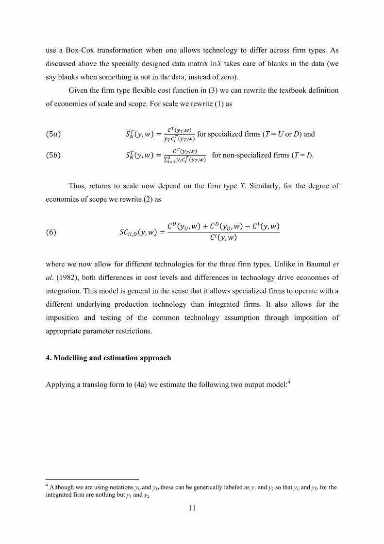
Given the firm type flexible cost function in (3) we can rewrite the textbook definition

of economies of scale and scope. For scale we rewrite (1) as

5 , ,

, for specialized firms (T = U or D) and

5 , ,

∑ , for non-specialized firms (T = I).

Thus, returns to scale now depend on the firm type T. Similarly, for the degree of

economies of scope we rewrite (2) as

6 , ,, , ,

,

where we now allow for different technologies for the three firm types. Unlike in Baumol et

al. (1982), both differences in cost levels and differences in technology drive economies of

integration. This model is general in the sense that it allows specialized firms to operate with a

different underlying production technology than integrated firms. It also allows for the

imposition and testing of the common technology assumption through imposition of

appropriate parameter restrictions.

4. Modelling and estimation approach

Applying a translog form to (4a) we estimate the following two output model:4

4 Although we are using notations yU and yD these can be generically labeled as y1 and y2 so that yU and yD for the integrated firm are nothing but y1 and y2.

12

7 ln ∗ ln ln ln12

ln12

ln

ln ln12

ln ln ln ln

ln ln

∗ ln ln12

ln

12

ln ln ln ln

∗ ln12

ln

12

ln ln ln ln

where C = total costs, yU = the quantity of upstream output, yD = the quantity of downstream

output, wk = the price of input k, M = the number of inputs used by integrated firms, G = the

number of inputs used by upstream firms, L = the number of inputs used by downstream

firms, and the Greek letters stand for the unknown population parameters.

The cost function is required to satisfy the following symmetry and linear

homogeneity (in input prices) constraints. Ignoring firm type indicators for ease of illustration,

these are:

(8) ; for firm types U, D, and I

(9) ∑ 1 ;∑ 0 forall ; ∑ 0

for firm types U, D, and I and for all j.

The linear homogeneity constraints are automatically imposed if we divide cost and

input prices by one arbitrarily chosen input price and drop the corresponding share equation.

13

Using Shephard's Lemma and the symmetry constraint we obtain share equation (10) for input

k.

(10) ∗ ln ln ∑ ln

∗ ln ∑ ln

∗ ln ∑ ln

We estimate this system of the cost function and share equations using the iterated

seemingly unrelated regression (SUR) technique (Zellner, 1962) after adding classical error

terms in the cost function and the cost share equations. The additional structure imposed by

the share equations makes the estimates more efficient as we add equations but do not

increase the number of parameters. All variables are demeaned so that the translog expansion

is around the sample mean across all firms and the first order coefficients can be interpreted

as elasticities at the sample mean.

If the parameters for each firm type technology are different, one can estimate them

separately by using the respective cost function and the share equations. However, a separate

regression approach always assumes the existence of different technologies without allowing

the possibility of hypothesis testing with regard to whether this assumption is valid.

Therefore, there are several advantages of our joint estimation approach over estimating

separate equations using data for each group. Firstly, only joint estimation is truly flexible in

the sense of allowing for both the possibility of a common technology or differences in firm

type technologies. Thus, even if there are enough observations in each group to separately

estimate each firm type technology, separate estimation may inappropriately impose different

technologies. In addition, with joint estimation we gain degrees of freedom by estimating all

three technologies jointly using all the data points. More precise estimates are obtained by

estimating all the parameters jointly and by using a system approach. The other significant

advantage is to test hypotheses across firm type technologies which cannot be done if these

technologies are estimated separately. In the joint estimation the implicit (default) assumption

is that the error variances and covariances (in the cost and share equations) are the same for

different firm type technologies. This can be easily generalized. In the separate estimation by

firm type the variances and covariances vary across firm type, and it is not possible to impose

restrictions across firm type technologies because they are estimated separately.

14

We perform the standard likelihood ratio test for inferences across groups. First, we

test whether restriction of the three firm type technologies to a single common technology is

valid. This common technology restriction is readily tested with a Likelihood ratio test by

imposing the following restrictions:

(11) :

These restrictions can be easily implemented by appropriately defining the data matrix

ln in the formulation ln , ln . The null hypothesis in (11) will be rejected if

the value of the test statistic:

(12) 2 )

(which is distributed as χ2 with degrees of freedom equal to number of restrictions) exceeds

the critical value of χ2 at a given level of significance. In (12) lnL and lnL are the log-

likelihood values for the restricted and unrestricted models.

Second, we can also separately test the restriction of the upstream (downstream) cost

function parameters to be equal to the integrated parameters. Thus, for example, to test

equivalence between the integrated firm parameters and the upstream firm parameters, we

would test a null hypothesis after dropping the second equality signs and setting all the

downstream only parameters to zero in (11).

5. Empirical application

The data is for US local government owned electric utilities. The data comprises three firm

types: upstream, integrated, and downstream. Our sample only includes conventional fossil-

fuel generators to avoid the bias from combining very different power generation technologies

15

as well as the confusion between vertical and horizontal integration economies when

interpreting the scope economies estimates (Arocena et al 2012). Downstream firms (D) are

pure power distributors, and integrated firms (I) engage in both activities, i.e. they generate

electricity from fossil fuels only and distribute the power. The data is an unbalanced panel for

the years 2000 to 2003. Table 1 illustrates the distribution of firms across the output space

(using electricity generation as upstream output and peak demand as downstream output). The

table gives the firm-year count by size bracket for the upstream and downstream activities.

The first row and first column give the counts of fully specialized firms and the diagonal

gives the count for fully integrated firms. There are 84 generation only and 148 distribution

only firm-year observations. Clearly the space between the diagonal and the two axes is less

densely populated. The total number of observations is 436.

[Place Table 1 about here]

We define the following variables. Our dependent variable, total cost (C) is measured

in US dollars and is the sum of capital, fuel and operating expenses. Operating expenses is the

sum of generation O&M, distribution O&M, Customer Accounts Expenses, Customer Service

& Informational Expenses, Sales Expenses and a pro-rata Admin & General O&M. We do not

include any transmission expenses. Capital expense is the capital stock multiplied by the

interest rate paid on long-term debt, plus depreciation expenses. The capital stock (K) is the

written down accounting value of fixed assets.

The single upstream output is net electricity generated (yG) and the single distribution

output is peak demand (yD). Given its complexity, it is common to model electricity

distribution as a multiple output technology including total distribution volumes, peak

demand, customers served, and/or distribution network length. However, while all these

output attributes are important, their inclusion also tends to cause serious multicollinearity

problems in estimation (Arocena et al. 2012; Kuosmanen, 2012). Given the purpose of this

paper, we have therefore decided on a more parsimonious model for two reasons. Firstly, to

avoid multicollinearity among second order terms due to strong correlation between

distribution output measures. Secondly, a simple model specification saves the estimation of

the large number of parameters typically required by the translog functional form when the

number of outputs increases. We have therefore chosen to focus on results based on a single

distribution output module with peak demand as distribution output on the logic that electrical

system design and its associated costs are to a larger extent driven by peak rather than average

16

loads. Further, in our application peak load is less correlated with the generation output than

power delivered or the number of consumers. In any case, we have experimented with

alternative models and the qualitative results are robust to alternative output specifications.

Finally, we include input prices for capital (wK), fuel (wF) and others (wO). The capital

price (wK) is capital expense divided by the capital stock (K). The fuel price (wF) is the fuel

expenditure divided by BTUs of fuel consumption. The final input variable that we define is

an Other Operating Costs (OC) variable. This variable includes both labour costs and other

operating costs excluding fuel expenses (e.g., outsourced services). Since detailed labour cost

data were not available we had to specify a single aggregate measure to capture these items.

The price of other (wO) is therefore defined as the state-level Census Bureau index of average

wages for all employees. The quantity measure for other outputs is then obtained implicitly by

deflating the cost measure by this price index. The price of other inputs is the numeraire used

to impose homogeneity in input prices.

We note that our model assumes that firms treat input prices and output quantities as

exogenous elements in their decision processes, thereby following the argument of Nerlove

(1963) and Christensen and Greene (1976). These two seminal studies of electricity industry

costs emphasize that, unlike for production function estimation where input quantities are

likely to be endogenous, cost function estimation is appropriate, given the reasonable

assumption that factor prices discussed above are determined in competitive markets or

through regulation, while electricity output is determined by consumer demand. Our sample

consists of regulated electric utilities that are obliged to serve all customers. Further, electric

power cannot be economically stored and thereby must be supplied on demand. Hence the

decision on outputs is exogenous to the firm. Thus, our empirical estimation approach builds

on a well-established literature that relies on dual cost function estimation in order to

specifically avoid the endogeneity problems that can affect production function estimation.

Table 2 provides summary statistics by firm type. The table shows that there are

important differences across the three firm types and that there are large variances within each

group. Dots indicate that a variable is not applicable to the type of firm. Regarding the outputs,

on average, generation only companies generate more than twice the amount of electricity as

integrated firms, arguably reflecting the effect that integrated firms can choose between

making and buying electricity. By contrast, the mean of the distribution output is virtually the

same for integrated firms and pure distributors.

We note that the publicly owned utilities in our sample are much smaller in terms of

output than the investor owned utilities employed in previous studies on US electric utilities

17

(e.g., Kaserman and Mayo, 1991; Kwoka 2002; Arocena et al., 2012, amongst others). Mean

prices of capital and other inputs are very similar across firm types. However, the estimated

price of fuel for integrated firms is more than twice the price for generation only firms

possibly reflecting bulk discounts for the latter or better procurement policies. The three cost

shares are roughly a third each for generation only firms. For the other two firm types the

shares of other inputs dominate.


6. Results

This section presents the parameter estimates and estimates for economies of scale and scope.

We normalize the data at the sample mean so that the first order coefficients of the translog

functions can be interpreted as elasticities (of the respective variables) at the mean of the data.

Table 3 gives the coefficient estimates for our three models. Under Model 1 we report the

estimates of the firm-type flexible technology model as detailed in equation (7) above. Note

that even though the estimates for the three firm types are given in different columns all the

parameters are estimated using a single regression. The first three rows in each column give

the firm type specific constant. Model 2 reports the parameter estimates from the conventional

common-technology model for the translog specification, where zeros were replaced by an

arbitrary small number (0.0001). Finally, Model 3 reports the parameters estimated allowing

for firm type technologies by using separate regressions for each firm type.

Statistics for the goodness of fit at the bottom of the Table 3 show that the R-squared

statistics (for the cost function equations) are very high for all models, but highest for Model

1. We observe that the coefficients, and hence estimated cost elasticities of Model 1 are very

close to those obtained from Model 3. In contrast, the individual coefficients for the

conventional common-technology specification with replacement of zero outputs with an

arbitrary number reported in Model 2 differ greatly.


Table 4 reports estimates of the economies of scale (S) and scope (SC) for the three

models. All estimates are at the sample mean. First consider the estimates for economies of

scale. For each model we report estimates of economies of scale for integrated firms as well

18

as estimates for the two types of specialized firms. The degree of scale economies defined

over the entire product set does not widely differ across models: all models provide evidence

for increasing returns to scale at the sample mean. Further, the scale economy estimates for

pure generators and distributors also consistently indicate increasing returns to scale under

both Models 1 and 3.

A further drawback of the conventional common-technology approach is that it is not

feasible to estimate the degree of scale economies for single output companies. Thus, the

standard approach here is to compute product-specific returns to scale, defined as the ratio of

the average incremental cost of a product to its marginal cost (Baumol et al., 1982), e.g.

(13)

)(

yC

AIC

yCy

yCyC

yCy

yICyS

i

i

ii

iN

ii

ii

for i = U,D

where ICi is the incremental cost of the product i, C(y) is the cost function, ii yyCyC /)(

is the marginal cost of product i, and yN-i is a vector with a zero component in place of yi and

components equal to those of y for the remaining products. That is, SU(y) (SD(y)) relates to the

increment in the firm’s cost which results from the addition of certain level of upstream

(downstream) product to the firm’s set of outputs, holding the magnitude of all other products

constant. Therefore the estimates for the common technology approach are not readily

comparable with the scale measures obtained from the other two models. Nevertheless the

estimates for scale for the specialized firm differ between Model 2 and Model 1 (Model 3). In

particular, the estimate for the upstream technology in Model 2 is unrealistically low.


We now turn to the estimates for economies of scope (SC), also shown in Table 4.

Models 1 and 3 report almost identical positive estimates at the sample mean. Thus, the

separate production of output vectors yG and yD increases the total cost by 4.3% to 4.4%. In

contrast, the estimated economies of scope are much stronger using a conventional common

technology approach with zero replacement. The estimate from Model 2 suggests that the

vertical separation of the average sample firm would increase total costs by 40.1%. In

quantitative terms such an estimate seems somewhat unrealistic but is within the range of

results reported in some previous studies for the US electric industry (e.g. Kaserman and

Mayo, 1991; Kwoka, 2002; Greer, 2008) who also use common-technology models.

19

We next perform statistical tests using Model 1 for the null hypothesis that the

different firm types share a common technology. We reject the null hypothesis in (11)] that

the technologies are the same across the different firm types at the 1 per cent level. Table 5

provides values of the relevant statistics. The first column tests equality of all coefficients

across the three firm types. The second and third columns show the test results for the

hypothesis that the technology of a specialized firm is the same as the technology for the

integrated firm. The second column for instance tests whether the parameters relating to the

upstream activity only are identical for upstream only and integrated firms. We stress that

inference on common technology is an important benefit of the firm type flexible technology

approach specified in (3), (4) and (7). While Model 3 demonstrates that it is possible to

estimate separate technologies for the different technologies with separate regressions, only

our flexible technology approach in Model 1 allows this direct statistical test of whether the

underlying cost function parameters for the three firm types are statistically different, and

therefore an appropriate specification. .

We finally note that we are aware that with a translog specification, differences in the

estimates between Model 1 (Model 3) and Model 2 are not only the result of the alternative

assumptions on the underlying technology across the three models. They may also be due to

the estimation bias created in Model 2 by replacing zero output values with arbitrary small

numbers, thereby implying that the scope economy estimates for this model are only

approximations, while those for Models 1 and 3 are fully consistent with the definition

provided in (6). There are of course alternative functional forms (e.g., quadratic) that are free

of such estimation bias under the conventional approach. In that case, any divergence between

the estimates between Model 1 and 2 would be exclusively due to differences in the modelling

of technology. Nevertheless, we emphasize that we have chosen the translog specification in

our empirical model precisely because we wish to show that our approach is particularly

useful for the translog form, which is normally considered to be problematic for the empirical

analysis of scope economies. In any case, it should be clear to the reader that the flexible

technology model is applicable to any functional form.5

5 In the interest of brevity, we do not report results for a quadratic form but the results are available upon request.

20


7. Conclusion

This paper has demonstrated the feasibility of estimating scope economies with a translog

modelling approach. This is accomplished by relaxing the generally accepted practice of

estimating a single cost function model, while assuming that both integrated and specialized

firms operate with the same production technology. The relaxation of this assumption

immediately eliminates the well-known zero output problem for translog estimation of

multiple output technologies, but also require the availability of data for both specialized and

integrated firms. However, this same data restriction also applies, for example, for standard

quadratic cost function models that impose a common technology, as it is generally accepted,

that even with a common technology assumption, a sufficient number of specialized firms is

required to validate the estimates. Thus, in contrast to previous translog papers, which have

relied on either cost complementarity results, or approximations of scale and scope economies

derived from zero replacement models, our flexible technology model demonstrates a readily

estimable model, which provides theoretically consistent estimates of scale and scope

economies. Thus contrary to accepted opinion, it is indeed feasible to accurately estimate

scope economies with a translog model, provided that it is a flexible model.

Within our sample of publicly owned US electric utilities, our modelling approach has

not only demonstrated the feasibility, but also the necessity of relaxing the standard practice

of assuming a common technology for specialized and integrated firms. While this conclusion

is application specific, we nonetheless suggest that a further substantial benefit of our flexible

technology model is its ability to allow readily applicable hypothesis testing of the

assumption that integrated and specialized firms share a common technology. Thus, a flexible

technology approach can also be applied with other functional forms such as the quadratic,

and will always allow for the empirical possibility of a common technology or significant

differences in technology between specialized and integrated firms.

We finally suggest that our results may have significant implications for the validity of

the past scope economy literature. Thus, if it can be more widely demonstrated that the

production technologies employed by specialized and integrated firms differ significantly we

would need to conclude that much of the past literature on scope economies has provided

biased results. Such a conclusion suggests a pressing need to reconsider the previous literature,

its empirical estimates, and the policy conclusions drawn from it.

21

References

Akridge, J.T., and Hertel, T.W. (1986). Multiproduct Cost Relationships for Retail Fertilizer

Plants, American Journal of Agricultural Economics 68: 928–938.

Arocena, P., Saal, D., and Coelli, T., (2012). Vertical and horizontal scope economies in the

regulated US electric power industry. Journal of Industrial Economics (forthcoming).

Battese, G. (1997). A note on the estimation of Cobb-Douglas production functions when

some explanatory variables have zero values. Journal of Agricultural Economics 48(2):

250-252.

Battese, G.; Malik, S.J. and Gill, M.A. (1996). An investigation of technical inefficiencies of

production of wheat farmers in four districts of Pakistan. Journal of Agricultural

Economics 47(2): 37-49.

Baumol, W.; Panzar, J.C. and Willig, R., 1982, Contestable Markets and the Theory of

Industry Structure. Harcourt Brace Jovanovich, San Diego, California, U.S.A.

Berger, A. N., Hanweck, G. A., and Humphrey, D. B. (1987). Competitive viability in

banking: Scale, scope, and product mix economies. Journal of Monetary Economics,

20(3): 501–520.

Bottasso, A., Conti, M., Piacenz, M., and Vannoni, D. (2011). The appropriateness of the

poolability assumption for multiproduct technologies: Evidence from the English water

and sewerage utilities. International Journal of Production Economics, 130(1): 112–117.

Caves, D. W., Christensen, L. R., and Tretheway, M. W. (1980). Flexible cost functions for

multiproduct firms. The Review of Economics and Statistics, 62(3): 477–481.

Charnes, A., Cooper, W. W., and Rhodes, E. (1978). Measuring the efficiency of decision

making units. European Journal of Operational Research, 2: 429–444.

Christensen, L. R., Jorgenson, D. W., and Lau, L. J. (1973). Transcendental logarithmic

production frontiers. The Review of Economics and Statistics, 55(1): 28–45.

Christensen, L.R. and Greene, H., 1976, ‘Economies of scale in the US electric power

generation,’ Journal of Political Economy, 84, pp. 655–677.

Cowing, T.G. and Holtmann, A.G. (1983). Multiproduct short-run hospital cost functions:

empirical evidence and policy implications from cross-section data. Southern Economic

Journal, 49, 637–653.

Färe, R. (1986). Addition and efficiency. The Quarterly Journal of Economics, 101(4): 861–

865.

22

Fraquelli, G., Piacenza, M., and Vannoni, D. (2005). Cost savings from generation and

distribution with an application to Italian electric utilities. Journal of regulatory

economics, 28(3): 289–308.

Fuss, M. A. and McFadden, D. (1978). Production economics: A dual approach to theory and

applications. Volume I: The theory of production. North-Holland: Amsterdam.

Fuss, M. A. and Waverman, L. (1981). Regulation and the multi-product firm: The case of

telecommunications in Canada, in Fromm, G. (ed.) Studies in Public Regulation MIT

Press, Cambridge, MA, USA.

Fuss, M.A. and Waverman, L. (2002) Econometric cost functions, in Cave, Majumdar and

Vogelsang (eds) Handbook of Telecommunications Economics Volume I: Structure,

Regulation and Competition, pp. 144-177. Elsevier: Amsterdam.

Garcia, S., Moreaux, M. and Reynaud, A. (2007) Measuring economies of vertical integration

in network industries: an application to the water sector, International Journal of

Industrial Organization, 25: 791-820

Gilligan T. and Smirlock M. (1984) An empirical study of joint production and scale

economies in commercial banking. Journal of Banking and Finance 8: 67–76

Gilsdorf, K., 1994, ‘Vertical integration efficiencies and electric utilities: a cost

complementarity perspective’, Quarterly Review of Economics and Finance, 34(3), pp.

261–282.

Goisis, G., Giorgetti, M.L., Parravicini, P., Salsano, F., Tagliabue, G. (2009) Economies of

scale and scope in the European banking sector, International Review of Economics 56

(3): 227–242.

Greer, M. (2008) A test of vertical economies for non–vertically integrated firms: The case of

rural electric cooperatives, Energy Economics, 30, pp. 679–687.

Gunning, T. S. and Sickles, R. C. (2009). A multi-product cost function for physician private

practices. Journal of Productivity Analysis, 35(2): 119–128.

Jara-Díaz, S., Ramos-Real, F. J. and Martínez-Budría, E. (2004). Economies of integration in

the Spanish electricity industry using a multistage cost function. Energy Economics,

26(6): 995–1013.

Jin,S.; Rozelle, S.; Alston, J. and Huang, J. (2005) Economies of scale and scope and the

economic efficiency of China’s agricultural research system. International Economic

Review, 46(3): 1033–1057.

23

Kaserman, D. L. and Mayo, J. W. (1991). The measurement of vertical economies and the

efficient structure of the electric utility industry. Journal of Industrial Economics, 39:

483–502.

Kim, Y.H. (1987) “Economies of Scale in Multi-Product Firms: An Empirical Analysis”,

Economica 54 (214), 185-206.

Kuosmanen, T. (2012). Stochastic semi-nonparametric frontier estimation of electricity

distribution networks: Application of the StoNED method in the Finnish regulatory

model-. Energy Economics, 30: article in press.

Kwoka, J. E. (2002). Vertical economies in electric power: evidence on integration and its

alternatives. International Journal of Industrial Organization, 20: 653–671.

Martínez-Budría, E., Jara-Díaz, S., and Ramos-Real, F. J. (2003). Adapting productivity

theory to the quadratic cost function: An application to the Spanish electric sector,

Journal of Productivity Analysis, 20(2): 213–229.

Mayo, J. (1984) Multiproduct monopoly, regulation and firm costs. Southern Economic

Journal, 51(1): 208–218.

Nerlove, M., 1963, ‘Returns to Scale in Electricity Supply,’ in Christ, C.F. (ed.),

Measurement in Economics. Studies in Mathematical Economics and Econometrics in

Memory of Yehuda Grunfeld, pp. 167–198 (Stanford University Press, Stanford,

California, U.S.A.).

Panzar, J. C. and Willig, R. D. (1981). Economies of scope. The American Economic Review,

71(2): 268–272.

Pulley, L. B. and Braunstein, Y. M. (1992). A composite cost function for multiproduct firms

with an application to economies of scope in banking. The Review of Economics and

Statistics, 74(2): 221–230.

Rezvanian, R. and Mehdian, S. (2002) An examination of cost structure and production

performance of commercial banks in Singapore. Journal of Banking and Finance 26:

79–98.

Röller, L. (1990) Modelling cost structure: the Bell System revisited. Applied Economics, 22:

1661–1674.

Weninger, Q. (2003). Estimating multiproduct costs when some outputs are not produced.

Empirical Economics, 28(4): 753–765.

Zellner, A. (1962). An efficient method of estimating seemingly unrelated regressions and

tests for aggregation bias. Journal of the American Statistical Association, 57(298):

348–368.

24

Table 1. Firm Count in Size Bracket

Distribution (GWh)

Generation (GWh) 0 <250 <500 <750 <1000 <2500 <5000 <7500 Total

0 0 47 39 24 5 21 4 8 148

<50 3 10 9 5 0 0 0 0 27

<250 9 9 42 2 3 10 0 0 75

<500 14 0 20 10 7 17 0 0 68

<750 7 0 3 4 4 4 0 0 22

<1000 13 0 0 0 0 5 0 0 18

<2500 28 0 4 4 6 11 8 0 61

<5000 10 0 0 0 2 1 4 0 17

Total 84 66 117 49 27 69 16 8 436

Table 2. Summary Statistics

All Generation Integrated Distribution mean sd mean sd mean sd mean sd

Total Cost (M.US dollars) 28.71 29.92 39.24 27.07 36.76 34.11 11.62 13.44

yG Net Generation (GWh) 753.46 847.61 1176.78 948.98 579.15 736.78 . . yD Peak load (MW) 192.87 236.08 . . 191.30 187.57 195.03 290.67 wK Price of Capital (Rate) 0.12 0.03 0.12 0.04 0.13 0.03 0.11 0.03 wF Price of Fuel (M/Mbtu) 2.25 1.73 1.28 0.67 2.65 1.87 . . wO Price of Other Inputs 0.92 0.12 0.92 0.12 0.92 0.13 0.91 0.11 Capital share 0.32 0.11 0.33 0.12 0.27 0.08 0.38 0.11 Fuel share 0.31 0.11 0.36 0.12 0.29 0.11 . . Other input share 0.48 0.16 0.32 0.13 0.44 0.10 0.62 0.11

Observations 436 84 204 148

25

Table 3. Parameter estimates Model 1 Model 2 Model 3

Integrated firms

Upstream firms

Downstream firms

All firms Integrated firms

Upstream firms

Downstream firms

I 0.099*** [0.03]

U −0.327*** [0.04]

D −0.841*** [0.03]

yG 0.457*** 0.866*** 0.546*** 0.453*** 0.882*** [0.02] [0.03] [0.0160] [0.0185] [0.0224]

yD 0.426*** 0.905*** 0.361*** 0.446*** 0.903*** [0.03] [0.02] [0.0227] [0.0291] [0.0288]

wK 0.274*** 0.308*** 0.399*** 0.279*** 0.275*** 0.298*** 0.403*** [0.01] [0.01] [0.01] [0.00756] [0.00601] [0.0119] [0.00966]

wF 0.293*** 0.397*** 0.296*** 0.294*** 0.406*** [0.00] [0.01] [0.00660] [0.00569] [0.00825]

yG2 0.105*** 0.038 0.0478*** 0.118*** 0.0243 [0.02] [0.03] [0.00190] [0.0141] [0.0173]

yD2 0.079 −0.252*** 0.0464*** 0.0836 −0.230*** [0.08] [0.03] [0.00330] [0.0507] [0.0500]

wK2 0.009 −0.112*** 0.136*** 0.00529 0.000186 −0.0776* 0.163*** [0.02] [0.03] [0.03] [0.0163] [0.0183] [0.0364] [0.0366]

wF2 0.146*** 0.206*** 0.0198*** 0.158*** 0.223*** [0.01] [0.01] [0.00472] [0.00584] [0.00928]

yD*yG −0.110*** −0.0215*** −0.118*** [0.03] [0.00123] [0.0200]

wK*yG −0.023** 0.011 0.00617** −0.0305*** 0.0150 [0.01] [0.01] [0.00238] [0.00623] [0.0107]

wK*yD 0.022 0.021** −0.00232* 0.0297** 0.0202* [0.01] [0.01] [0.000955] [0.00950] [0.00868]

wF*yG 0.105*** 0.042*** 0.00516* 0.115*** 0.0359*** [0.00] [0.01] [0.00215] [0.00561] [0.00750]

wF*yD −0.083*** −0.0047*** −0.0987*** [0.01] [0.000827] [0.00838]

wF*wK −0.044*** −0.036** −0.0248*** −0.0571*** −0.0609*** [0.01] [0.01] [0.00522] [0.00746] [0.0127]

Constant 0.109*** 0.0899*** −0.332*** −0.855*** [0.0226] [0.0234] [0.0262] [0.0412]

Observations 436 436 204 84 148

RSS 32.90 37.82 12.46 4.26 16.13

RMSE 0.27 0.29 0.25 0.23 0.33

Ll 1104.55 812.22 612.22 241.09 82.86

R-squared 0.95 0.92 0.92 0.93 0.87

Standard errors in brackets * p < 0.05, ** p < 0.01, *** p < 0.001

26

Table 4. Economies of scale and scope at the sample mean

Table 5. Inference on Common Technology

All Upstream Downstream

N 444 444 444

Chi2 1297.15 526.32 2928.23

DF 27 26 28

p 0.00 0.00 0.00

Null hypothesis is that single technology is nested in separate technologies

Model 1: Firm-type flexible technology

S (I) 1.132 S (U) 1.155 S (D) 1.105 SC 0.043

Model 2: Common Technology

S (I) 1.102 S (U) 0.701 S (D) 1.293 SC 0.401

Model 3: Separate regressions

S (I) 1.112 S (U) 1.134 S (D) 1.108 SC 0.044

Ifo Working Papers

No. 141 Potrafke, N. und M. Reischmann, Fiscal Equalization Schemes and Fiscal Sustainability,

September 2012.

No. 140 Fidrmuc, J. and C. Hainz, The Effect of Banking Regulation on Cross-Border Lending,

September 2012.

No. 139 Sala, D. and E. Yalcin, Export Experience of Managers and the Internationalization of

Firms, September 2012.

No. 138 Seiler, C., The Data Sets of the LMU-ifo Economics & Business Data Center – A Guide

for Researchers, September 2012.

No. 137 Crayen, D., C. Hainz and C. Ströh de Martínez, Remittances, Banking Status and the

Usage of Insurance Schemes, September 2012.

No. 136 Crivelli, P. and J. Gröschl, The Impact of Sanitary and Phytosanitary Measures on Market

Entry and Trade Flows, August 2012.

No. 135 Slavtchev, V. and S. Wiederhold, Technological Intensity of Government Demand and

Innovation, August 2012.

No. 134 Felbermayr, G.J., M. Larch and W. Lechthaler, The Shimer-Puzzle of International

Trade: A Quantitative Analysis, August 2012.

No. 133 Beltz, P., S. Link and A. Ostermaier, Incentives for Students: Evidence from Two Natural

Experiments, August 2012.

No. 132 Felbermayr, G.J. and I. Reczkowski, International Student Mobility and High-Skilled

Migration: The Evidence, July 2012.

No. 131 Sinn, H.-W., Die Europäische Fiskalunion – Gedanken zur Entwicklung der Eurozone,

Juli 2012.

No. 130 Felbermayr, G.J., A. Hauptmann and H.-J. Schmerer, International Trade and Collective

Bargaining Outcomes. Evidence from German Employer-Employee Data, March 2012.

No. 129 Triebs, T.P. and S.C. Kumbhakar, Management Practice in Production, March 2012.

No. 128 Arent, S., Expectations and Saving Behavior: An Empirical Analysis, March, 2012.

No. 127 Hornung, E., Railroads and Micro-regional Growth in Prussia, March, 2012.

No. 126 Seiler, C., On the Robustness of the Balance Statistics with respect to Nonresponse,

March 2012.

No. 125 Arent, S., A. Eck, M: Kloss and O. Krohmer, Income Risk, Saving and Taxation: Will

Precautionary Saving Survive?, February 2012.

No. 124 Kluge, J. and R. Lehmann, Marshall or Jacobs? Answers to an Unsuitable Question from

an Interaction Model, February 2012.

No. 123 Strobel, T., ICT Intermediates, Growth and Productivity Spillovers: Evidence from

Comparison of Growth Effects in German and US Manufacturing Sectors, February 2012.

No. 122 Lehwald, S., Has the Euro Changed Business Cycle Synchronization? Evidence from the

Core and the Periphery, January 2012.

No. 121 Piopiunik, M. and M. Schlotter, Identifying the Incidence of “Grading on a Curve”: A

Within-Student Across-Subject Approach, January 2012.

No. 120 Kauppinen, I. and P. Poutvaara, Preferences for Redistribution among Emigrants

from a Welfare State, January 2012.

No. 119 Aichele, R. and G.J. Felbermayr, Estimating the Effects of Kyoto on Bilateral Trade

Flows Using Matching Econometrics, December 2011.

No. 118 Heid, B., J. Langer and M. Larch, Income and Democracy: Evidence from System

GMM Estimates, December 2011.

No. 117 Felbermayr, G.J. and J. Gröschl, Within US Trade and Long Shadow of the American

Secession, December 2011.

No. 116 Felbermayr, G.J. and E. Yalcin, Export Credit Guarantees and Export Performance:

An Empirical Analysis for Germany, December 2011.

estimating economies of scale and scope with flexible technology

Documents