estimating latent people flow without tracking individuals

Estimating Latent People Flow without Tracking Individuals

Yusuke Tanaka1, Tomoharu Iwata2, Takeshi Kurashima1, Hiroyuki Toda1, Naonori Ueda2,31 NTT Service Evolution Laboratories, Kanagawa 239-0847, Japan

2 NTT Communication Science Laboratories, Kyoto 619-0237, Japan3 RIKEN Center for AIP, Tokyo 103-0027, Japan

{tanaka.y, iwata.tomoharu, kurashima.takeshi, toda.hiroyuki, ueda.naonori}@lab.ntt.co.jp

AbstractAnalyzing people flows is important for better nav-igation and location-based advertising. Since thelocation information of people is often aggregatedfor protecting privacy, it is not straightforward toestimate transition populations between locationsfrom aggregated data. Here, aggregated data areincoming and outgoing people counts at each lo-cation; they do not contain tracking informationof individuals. This paper proposes a probabilisticmodel for estimating unobserved transition popula-tions between locations from only aggregated data.With the proposed model, temporal dynamics ofpeople flows are assumed to be probabilistic diffu-sion processes over a network, where nodes are lo-cations and edges are paths between locations. Bymaximizing the likelihood with flow conservationconstraints that incorporate travel duration distri-butions between locations, our model can robustlyestimate transition populations between locations.The statistically significant improvement of ourmodel is demonstrated using real-world datasets ofpedestrian data in exhibition halls, bike trip dataand taxi trip data in New York City.

1 IntroductionWith recent advances in wireless and mobile networks, lo-cation information of people can be recorded in a variety ofspaces such as exhibition halls, shopping malls, amusementparks, and urban cities. It is important to understand peo-ple’s mobility patterns in these spaces, because it providesuseful knowledge for optimizing navigation systems [Huangand Gartner, 2010], travel route recommendation [Kurashimaet al., 2010], location-based mobile advertising [Dhar andVarshney, 2011], urban planning [Yuan et al., 2012], and dis-aster management [Song et al., 2014]. For example, analyz-ing the routes of people helps to guide them to the locationsof interest, and determine which advertisement to serve to thevisitors to suit their current locations.Many statistical methods that analyze trajectory data have

been proposed to understand people’s mobility patterns [Gi-

Incoming count Outgoing count

location 1

location 2

location 3

location 1

location 2

location 3

location 1

location 2

location 3

t-1 t t+1

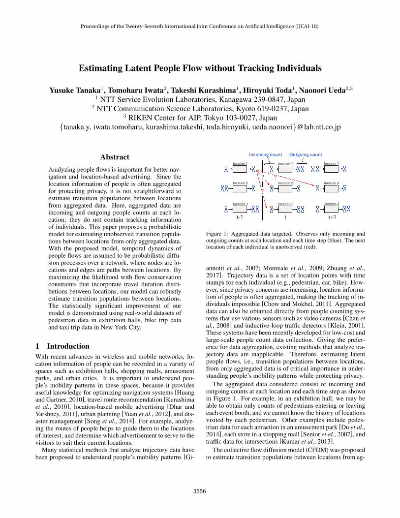
Figure 1: Aggregated data targeted. Observes only incoming andoutgoing counts at each location and each time step (blue). The nextlocation of each individual is unobserved (red).

annotti et al., 2007; Monreale et al., 2009; Zhuang et al.,2017]. Trajectory data is a set of location points with timestamps for each individual (e.g., pedestrian, car, bike). How-ever, since privacy concerns are increasing, location informa-tion of people is often aggregated, making the tracking of in-dividuals impossible [Chow and Mokbel, 2011]. Aggregateddata can also be obtained directly from people counting sys-tems that use various sensors such as video cameras [Chan etal., 2008] and inductive-loop traffic detectors [Klein, 2001].These systems have been recently developed for low-cost andlarge-scale people count data collection. Giving the prefer-ence for data aggregation, existing methods that analyze tra-jectory data are inapplicable. Therefore, estimating latentpeople flows, i.e., transition populations between locations,from only aggregated data is of critical importance in under-standing people’s mobility patterns while protecting privacy.The aggregated data considered consist of incoming and

outgoing counts at each location and each time step as shownin Figure 1. For example, in an exhibition hall, we may beable to obtain only counts of pedestrians entering or leavingeach event booth, and we cannot know the history of locationsvisited by each pedestrian. Other examples include pedes-trian data for each attraction in an amusement park [Du et al.,2014], each store in a shopping mall [Senior et al., 2007], andtraffic data for intersections [Kumar et al., 2013].The collective flow diffusion model (CFDM) was proposed

to estimate transition populations between locations from ag-

Proceedings of the Twenty-Seventh International Joint Conference on Artificial Intelligence (IJCAI-18)

3556

gregated data [Kumar et al., 2013]. CFDM is learned by max-imizing a likelihood subject to constraints that represent peo-ple flow conservation. The constraint states that all peoplewho leave a location at time step t always arrive at anotherlocation at the next time step, t+1. However, this assumptionis too restrictive for many real-world applications, mainly be-cause we do not always have a large enough number of sensordevices to cover large-scale spaces: People might be movingthrough passages where no sensor devices are placed at anobservation time step. In that case, the people are not ob-served in any location, and CFDM fails to estimate transitionpopulations accurately as it assumes that everyone is in oneor other of the observed locations at the next time step.The purpose of this paper is to robustly estimate unob-

served transition populations between locations in practicalsituations, that is, the observation range is limited and somepeople are not observed in any location in some time periods.In order to achieve our purpose, we propose a new probabilis-tic model that incorporates people’s travel duration betweenlocations. This is, however, quite challenging to implement,because travel duration between locations is not present in theaggregated data, and, moreover, people are heterogeneous sotravel duration depends on the individual. For example, in anexhibition hall, some people might directly visit their next lo-cation, but others might take a rest before arriving at anotherlocation; in an urban city, moving speeds might depend onthe means of transport (e.g., walking, bike, car).With the proposed model, the temporal dynamics of peo-

ple flows are assumed to be probabilistic diffusion processesover a network, where the nodes are locations (e.g., boothsand shops) and the edges are paths between these locations(e.g., passages and roads). People diffuse from node to nodeaccording to transition probabilities that depend on their lo-cations. Since the transition populations between locationsare not observed, we treat them as latent variables. Our keyidea is to treat travel duration as random variable that followsa probability distribution. This enables us to capture the het-erogeneity in travel duration among individuals. The distri-butions of travel duration are incorporated into the constraintsthat represent flow conservation; they aim to model that peo-ple who left one location in one time step and arrived at an-other location after some delay. We develop an efficient in-ference algorithm to estimate the transition probabilities, thetransition populations, and the travel duration distributions.We show the effectiveness of our model on real-world

datasets, pedestrian location logs from large-scale exhibitionhalls, and bike trip data and taxi trip data in New York City.First, we show that our model achieves high estimation per-formance for the transition populations between locations.Second, we show that our model precisely captures the travelduration distributions between locations. Third, by using theestimated transition populations, we show that our model cananalyze the routes of pedestrians in exhibition halls that arelikely to be chosen by visitors without tracking individuals.The major contributions of this paper include:• We propose a probabilistic model that incorporates

travel duration distributions for robustly estimating un-observed transition populations between locations fromonly aggregated data.

• We develop an efficient inference algorithm to learn thetransition probabilities, the transition populations, andthe travel duration distributions.

• Experiments on multiple real-world datasets show thatour proposed model achieves statistically significant im-provement over baseline methods.

2 Related WorkA number of works have been published recently that use thelatest trends (e.g., deep learning) for analyzing aggregateddata such as population or inflow and outflow at each loca-tion [Hoang et al., 2016; Zhang et al., 2017; Yao et al., 2018].These works can predict the population or inflow and outflowin the future with consideration of some external factors (e.g.,weather). They cannot, however, estimate the transition pop-ulations between locations from inflow and outflow, whichis the task considered in this paper. The task of estimatingthe transition populations between locations is important forbetter understanding people’s mobility patterns; for example,it is useful for finding the popular routes of pedestrians inexhibition halls. While the method of [Xu et al., 2017] canrecover user trajectories given aggregated data and transitionprobabilities. The transition probabilities must be manuallyset by using other information such as distances between lo-cations. In other words, the method cannot estimate the tran-sition populations between locations from only aggregateddata. Different from that method, our model can estimatenot only the transition populations but also transition proba-bilities from only aggregated data. What is more, our modelalso enables us to estimate the travel duration distributions, afunction not considered in the previous method.Collective graphical models (CGMs) [Sheldon and Di-

etterich, 2011] have been recently developed as a generalframework for analyzing aggregated data. The models havebeen applied for modeling contingency tables [Sheldon andDietterich, 2011] and bird migration [Sheldon et al., 2008].Prior works provide efficient inference techniques for CGMsbased on maximum a posteriori [Sheldon et al., 2013],MCMC sampler [Sheldon and Dietterich, 2011], messagepassing [Sun et al., 2015], and variational Bayesian infer-ence [Iwata et al., 2017]. The collective flow diffusionmodel (CFDM) [Kumar et al., 2013] is the first applica-tion of efficient inference techniques developed for CGMsto the transportation domain. By maximizing a likelihoodsubject to constraints that represent people flow conserva-tion, this model can estimate transition populations betweenlocations from only aggregated data [Kumar et al., 2013;Du et al., 2014]. However, CFDM does not consider peo-ple’s travel duration between locations, which is importantfor modeling the temporal dynamics of people flows. Theproposed model is an extension of CFDM, and incorporatestravel duration distributions into the constraints that representflow conservation. Our model can estimate the transition pop-ulations between locations with consideration of the travelduration. Therefore, our model more precisely estimates tran-sition populations between locations than previous models.Information diffusion models are related to our work, be-

cause their main goal is to estimate latent flows of a piece of


3557

Symbol DescriptionV set of locationsi location, i ∈ VEi set of locations that are accessible from location iT #observation time stepsNout

t,i #outgoing people from location i at time step t,Nout

t,i ≥ 0N in

t,i #incoming people to location i at time step t,N in

t,i ≥ 0Mtij transition population who leave location i at time

step t and whose next location is j,Mtij ≥ 0θij transition probability that people leave location i

and move to location j, θij ≥ 0,∑

j∈Eiθij = 1

αji parameter of travel duration distribution fromlocation j to i, αji > 0

λ hyperparameter for controlling the penalty, λ ≥ 0

Table 1: Notation

information over a network. These models have been used foranalyzing the spread of information [Rodriguez et al., 2011;Kurashima et al., 2014] and user influence [Iwata et al., 2013;Tanaka et al., 2016] over social networks. These models in-corporate a continuous time distribution to model the tempo-ral dynamics of information flows, with the aim of describ-ing the spread of information from node to node with de-lays over time. However, in analyzing information flows, itis not necessary to consider flow conservation, a critical fac-tor in modeling the temporal dynamics of people flows basedon aggregated data. Our model can infer latent people flowsfrom only aggregated data by considering the flow conserva-tion constraints that incorporate travel duration distributions.

3 Problem FormulationIn this section, we detail the aggregated data considered here,and define our problem of estimating latent people flows. Thenotations used in this paper are listed in Table 1.Aggregated data: We illustrate an example of aggregated

data for the three locations in the upper part of Figure 2. Thedata consist of incoming and outgoing counts at each loca-tion and each time step. Let Nout

t,i be the count of outgo-ing people from location i at time step t, and N in

t,i be thecount of incoming people to location i at time step t. Sup-pose that we are given a set of outgoing counts Nout ={Nout

t,i |t = 0, . . . , T −1, i ∈ V} and a set of incoming countsNin = {N in

t,i|t = 1, . . . , T, i ∈ V}, where T is the numberof observation time steps and V is the set of locations. Theaggregated data of individuals (e.g., pedestrians, cars, bikes)can be gathered using various methods such as Wi-Fi [Musaand Eriksson, 2012], Bluetooth [Kotanen et al., 2003], andvideo-based people counting systems [Chan et al., 2008].Problem: Our problem of estimating latent people flows,

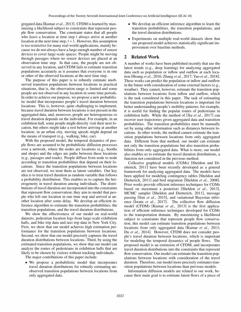
i.e., transition populations between locations, is formulatedas follows. Figure 2 illustrates the studied problem for thecase of three locations. Suppose that we have a set of incom-ing and outgoing counts at each location and each time step.We would like to estimate the transition population betweenlocations at each time step,Mtij , which is the number of peo-

inc

om

ing

co

un

to

utg

oin

g c

ou

nt location 1 location 2 location 3

time step time steptime step time step

Infer

location 1 location 1

location 2 location 3 location 2 location 3

t=0 t=1

transition population

Figure 2: Illustration of the studied problem. (Upper figures) Theaggregated data at each location. (Lower figures) Visualization ofthe estimated transition populations between locations at each timestep, where arrow width is proportional to the transition population.

ple who left location i at time step t and whose next locationwas j. Our goal is to infer a set of transition populationsM = {Mtij |t = 0, . . . , T − 1, i ∈ V, j ∈ Ei}, where Ei isthe set of locations that are accessible from location i; peoplein location i can move only to the linked locations j ∈ Ei.

4 ModelWe propose a probabilistic model that incorporates people’stravel duration between locations for estimating unobservedtransition populations between locations from only aggre-gated data. Modeling the travel duration between locations isexpected to estimate the transition populations more robustlyin practical situations, that is, the observation range is limitedand some people are not observed in any location in sometime periods.In the proposed model, the temporal dynamics of people

flows are assumed to be probabilistic diffusion processes overa network, where the nodes are locations and the edges arepaths between these locations. If the network structure suchas road networks or a set of neighbor information is unknown,our model works by assuming a complete graph among loca-tions. We assume that people diffuse from node to node inaccordance with location-dependent transition probabilities.Let θij ≥ 0 be the transition probability that people leave lo-cation i and move to location j, where

∑j∈Ei

θij = 1. Giventhe outgoing countNout

t,i and the transition probabilities θi ={θij |j ∈ Ei}, transition population Mti = {Mtij |j ∈ Ei} isgiven by the following multinomial distribution,

P (Mti|Noutt,i ,θi) =

Noutt,i !∏

j∈EiMtij !

∏j∈Ei

θMtij

ij . (1)

Since we cannot obtain the tracking information of individu-als in our aggregated data setting, Mti is unobserved. There-fore, we treat it as a latent variable. Transition population


3558

Mti satisfies the following two relations that represent out-going and incoming flow conservation:

Noutt,i =

∑j∈Ei

Mtij , (2)

N int,i =

∑j∈Ei

t−1∑τ=0

F (∆t,τ ;αji)Mτji. (3)

The outgoing flow conservation (2) indicates that the sum ofpeople leaving location i at time step t equals the observedoutgoing count at the same time step. The incoming flowconservation (3) indicates that the weighted sum of peopleleaving location j before time step t equals the observed in-coming count at time step t. Weight F (∆t,τ ;αji) is travelduration probability, which is the probability that people wholeft location j at time step τ arrive at location i at time stept. Here, ∆t,τ = t − τ is travel duration and αji is a param-eter of the probability distribution. Details of F (∆t,τ ;αji)are given in the following paragraphs. The travel duration istreated as a random variable that follows the probability dis-tribution; it is not a point estimate. This enables us to capturethe heterogeneity in travel duration among individuals.To derive the travel duration probability F (∆t,τ ;αji),

we first introduce continuous travel duration distributionf(∆;αji) as the probability density function of travel dura-tion∆ from location j to i given parameter αji, where∆ > 0is a continuous random variable. Note that our model does notdepend on the particular choice of the travel duration distri-bution. The travel duration probability F (∆t,τ ;αji) is calcu-lated by the following integral of f(∆;αji) over the intervalfrom ∆t,τ − 1 to∆t,τ :

F (∆t,τ ;αji) =

∫ ∆t,τ

∆t,τ−1

f(∆;αji)d∆. (4)

Though our model can use any distribution as f(∆;αji),for simplicity we consider the well-known one-parameter dis-tribution, i.e., Rayleigh distribution, which is widely used forassessing the duration time in various fields such as user mod-eling [Wang et al., 2008] and information diffusion model-ing [Rodriguez et al., 2011]. Figure 3 illustrates an examplewhen using the Rayleigh distribution. The travel duration dis-tribution is as follows:

f(∆;αji) =∆

α2ji

exp(− ∆2

2α2ji

), (5)

the red line in Figure 3. Here, αji > 0. The travel durationprobability is given by

F (∆t,τ ;αji) = exp(− (∆t,τ − 1)2

2α2ji

)− exp

(− (∆t,τ )

2

2α2ji

),

(6)the red area in Figure 3: The probability that people who leftlocation j at time step τ arrive at location i at time step t.

5 InferenceGiven outgoing counts Nout and incoming counts Nin, weestimate the latent transition populations M, the transition

de

nsi

ty

travel duration Δ

Figure 3: Travel duration probability from location j to i, where∆t,τ is the time difference between outgoing time τ and incomingtime t. The gray vertical lines are spaced by unit time steps.

probabilities Θ = {θi|i ∈ V}, and the parameters of travelduration distributions A = {αji|j ∈ V, i ∈ Ej} by maxi-mizing the likelihood with the flow conservation constraints.The log-likelihood ofM is given by

logP (M|Nout,Θ)

∝T−1∑t=0

∑i∈V

∑j∈Ei

(− logMtij ! +Mtij log θij

)

≈T−1∑t=0

∑i∈V

∑j∈Ei

((1 + log θij)Mtij −Mtij logMtij

), (7)

where logNti! is omitted since it does not depend onM, andwe employ Stirling’s approximation, log n! ≈ n log n− n, inorder to calculate logMtij ! efficiently [Sheldon et al., 2013].The parameters are estimated by maximizing the approximatelog-likelihood (7) subject to constraints (2) and (3). The con-straints might not strictly hold in real-world data, because theobservations are noisy. To handle noisy observations, we treatthe constraints as soft constraints, where the squared differ-ence between the left- and right-hand sides in each of (2)and (3) are minimized. Then, the objective function to bemaximized is described as follows:

J (M,Θ,A)

=T−1∑t=0

∑i∈V

[∑j∈Ei

((1 + log θij)Mtij −Mtij logMtij

)− λ

2∥Nout

t,i −∑j∈Ei

Mtij∥2

− λ

2∥N in

t+1,i −∑j∈Ei

t∑τ=0

F (∆t+1,τ ;αji)Mτji∥2]. (8)

Here, λ ≥ 0 is a hyperparameter that controls the penalty forviolating the constraints and ∥ · ∥ is the Euclidean norm. Weupdate each parameter M, Θ and A alternately as describedin the following paragraphs.Update ofM: Given current estimates Θ and A, we arrive


3559

Algorithm 1: Inference procedure for our model.

Input :Nin,Nout,V, {Ei}i∈V, T , λOutput:M,Θ, A1: Initialize M,Θ, A2: repeat3: UpdateM by solving (9)4: for i ∈ V do5: for j ∈ Ei do6: Update θij by (10)7: end for8: end for9: UpdateA by solving (11)10: until Convergence

at the following optimization problem:

maximizeM

J (M, Θ, A)

subject to Mtij ≥ 0, t = 0, . . . , T − 1, i ∈ V, j ∈ Ei.(9)

We solve the optimization problem by using the L-BFGS-Bmethod [Byrd et al., 1995].Update of Θ: The estimates of Θ are obtained in closed

form by maximizing (8) given current estimates M as fol-lows:

θij =

∑T−1t=0 Mtij∑T−1

t=0

∑j∈Ei

Mtij

. (10)

Update ofA: Given current estimates M and Θ, we solvethe following optimization problem:

maximizeA

J (M, Θ,A)

subject to αji > 0, j ∈ V, i ∈ Ej ,(11)

by using the L-BFGS-B method [Byrd et al., 1995]. We itera-tively update each parameter until the value of (8) converges.Our inference procedure is shown in Algorithm 1, which al-ways converges and guarantees that the local optima of the re-spective parameters are obtained by setting λ to a fixed value.Validation of λ: Hyperparameter λ can be determined by

the following validation procedure: (a) learn the model pa-rameters by Algorithm 1 with each candidate value of λ; (b)predict the incoming counts at the next time step; (c) choosethe value based on prediction performance in the trainingdata. Given the preceding outgoing counts, the predicted in-coming counts in location i at the next time step are givenby

N int+1,i =

∑j∈Ei

t∑τ=0

F (∆t,τ ; αji)θjiNoutτ,j . (12)

6 Experiments6.1 Data DescriptionWe evaluated the proposed model using real-world pedes-trian location logs collected in exhibition halls. The data wascollected at an event that attracted large crowds, Niconico

Data Pedestrian data Bike trip data Taxi trip dataArea/Date Hall 1 Hall 2 Hall 3 Hall 4 Mar. 1 Jun. 1 Mar. 1 Jun. 1#outgoing 30,606 34,750 15,448 10,990 14,366 18,961 201,440 196,101#incoming 30,606 34,750 15,448 10,990 14,640 19,312 204,476 199,232

Table 2: The total sum of incoming and outgoing counts

Chokaigi 2016 1, held at Makuhari Messe located near Tokyo,Japan from 10:00 to 18:00 on April 29th. The event site wascomposed of four exhibition halls, Hall 1, Hall 2, Hall 3 andHall 4 with sizes of 186.3m × 124.8m, 183.2m × 124.8m,127.6m × 124.8m, and 190.9m × 108.3m, respectively. Thenumber of event booths, |V |, in Hall 1, Hall 2, Hall 3 andHall 4 were 38, 27, 10, and 9, respectively. We gatheredpedestrian location logs using Bluetooth beacons which wereplaced at each booth. The technology enables us to observethe times at which each user entered or left the observationrange (at most 10 – 15 meters). The data consist of 3,727mobile users who agreed to provide detailed information oflocation over time. The original data contains time stampsof arrival and departure at booths for each user; users can betracked over time. Note that the tracking information of userswas used only for evaluating the estimation performance fortransition populations and travel duration probabilities; wedid not use the tracking information in the inference process.In this experiment, we created aggregated incoming and out-going pedestrian counts at each booth, where the time inter-val was 3 minutes. The number of observation time steps was160. Ei was a set of edges assuming a complete graph for alldatasets. The total sum of incoming and outgoing pedestriansat all booths in each hall are shown in Table 2.To additionally validate the performance of our model, we

used two public datasets, bike trip data 2 and taxi trip data 3

in New York City. The data is a set of trip records consistingof: trip id, pickup location, dropoff location, pickup date andtime, and dropoff date and time. Note that the data consist oflocation information only when people started and finishedthe trips; the trajectories during the trips are not recorded.We used the data from 8:00 to 24:00 on March 1st and June1st, and created gridded incoming and outgoing count data,where the time interval in both datasets was 10 minutes. Thenumber of observation time steps was 96. The grid sizes inthe bike trip data and taxi trip data were 2km× 2km (12× 12grid cells) and 3km × 3km (18 × 18 grid cells), respectively.Here, we omitted grid cells if their incoming and outgoingcounts were lower than a threshold. Then, bike trip data andtaxi trip data held 11 and 14 grid cells, respectively. Ei was aset of edges assuming a complete graph for all datasets. Thetotal sum of incoming and outgoing bikes/taxis at overall gridcells on each date are shown in Table 2.

6.2 Quantitative EvaluationTransition Population EstimationWe evaluated our model in terms of its performance in esti-mating the transition populations M. The evaluation metric

1http://www.chokaigi.jp/2016/en/2https://www.citibikenyc.com/system-data3http://www.nyc.gov/html/tlc/html/about/trip record data.shtml


3560

Data Pedestrian data Bike trip data Taxi trip dataArea/Date Hall 1 Hall 2 Hall 3 Hall 4 Mar. 1 Jun. 1 Mar. 1 Jun. 1Proposed 1.237 ± 0.024 1.028 ± 0.014 0.784 ± 0.034 0.675 ± 0.030 0.621± 0.015 0.704± 0.021 0.443± 0.006 0.454 ± 0.006CFDM 1.370 ± 0.030 1.140 ± 0.013 0.828 ± 0.038 0.709 ± 0.030 0.648± 0.015 0.740± 0.021 0.463± 0.006 0.469 ± 0.006

Popularity 1.751 ± 0.012 1.594 ± 0.013 1.180 ± 0.019 0.848 ± 0.025 0.724± 0.016 0.790± 0.021 0.510± 0.009 0.520 ± 0.008Uniform 1.835 ± 0.011 1.676 ± 0.012 1.210 ± 0.019 1.221 ± 0.024 1.031± 0.013 1.081± 0.018 0.983± 0.010 0.987 ± 0.009

Table 3: NMAE L1 and standard errors for the estimation of transition populations in the real-world datasets.

is the following normalized mean absolute error (NMAE) intransition populations:

L1 =1

T

T−1∑t=0

∑i∈V

∑j∈Ei

|M⋆tij − Mtij |∑

i∈V

∑j∈Ei

M⋆tij

, (13)

where M⋆tij is the true transition population leaving location

i at time step t and whose next location is j; Mtij is its esti-mate. We compared our proposed model with the collectiveflow diffusion model (CFDM) [Kumar et al., 2013]. Differ-ent from our model, CFDM does not consider travel durationbetween locations. In addition, we compared our proposedmodel with the following two baseline methods: Popularityand Uniform methods. Popularity assumes that people moveto other locations in proportion to location popularity regard-less of current locations; the estimated transition populationis given by

Mtij = Noutt,i ×

∑T−1t=0 N in

t+1,j∑T−1t=0

∑j∈Ei

N int+1,j

. (14)

Uniform estimates transition populations using a discrete uni-form distribution; it assumes that people move to neighbor lo-cations with equal probability 1/|Ei|. For our model, hyper-parameter λ was set to the best value based on the validationprocedure described in Section 5; λwas chosen from 0.1, 0.2,0.5, 1, 2, and 5. We used a Rayleigh distribution for modelingtravel duration distribution as shown in Section 4.Table 3 shows NMAE L1 of the proposed model, CFDM,

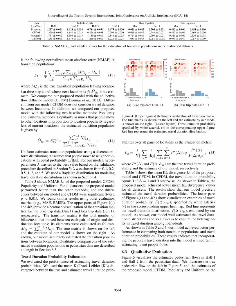
Popularity and Uniform. For all datasets, the proposed modelperformed better than the other methods, and the differ-ences between our model and CFDM were significant (t-test,p < 0.01). We found similar results using other evaluationmetrics (e.g., MAE, RMSE). The upper parts of Figure 4(a)and 4(b) provide a heatmap visualization of the transition ma-trix for the bike trip data (Jun.1) and taxi trip data (Jun.1),respectively. The transition matrix is the total number ofbikes/taxis that moved between each pair of origin and des-tination locations; its elements were calculated as follows:Mij =

∑T−1t=0 Mtij . The true matrix is shown on the left

and the estimate of our model is shown on the right. Asshown, our model accurately estimated the transition popula-tions between locations. Qualitative comparisons of the esti-mated transition populations in pedestrian data are describedat length in Section 6.3.

Travel Duration Probability EstimationWe evaluated the performance of estimating travel durationprobabilities. We used the mean Kullback-Leibler (KL) di-vergence between the true and estimated travel duration prob-

destination

ori

gin

pro

ba

bil

ity

travel duration(time step)

1.0

00 5 0 5

1.0

0.8

0.6

0.4

0.2

0.0

✕103

(a) Bike trip data (Jun. 1)

destination

ori

gin

pro

ba

bil

ity

travel duration(time step)

1.0

00 5 0 5

1.25

1.00

0.75

0.50

0.25

0.00

✕104

(b) Taxi trip data (Jun. 1)

Figure 4: (Upper figures) Heatmap visualization of transition matrix.The true matrix is shown on the left and the estimate by our modelis shown on the right. (Lower figures) Travel duration probabilityspecified by white asterisk (∗) in the corresponding upper figure.Red line represents the estimated travel duration distribution.

abilities over all pairs of locations as the evaluation metric:

L2 =1

|V|∑j∈V

1

|Ej |∑i∈Ej

T∑∆=1

P ⋆(∆) logP ⋆(∆)

F (∆; αji), (15)

where P ⋆(∆) and F (∆; αji) are the true travel duration prob-ability and the estimate of our model, respectively.Table 4 shows the mean KL divergence L2 of the proposed

model and CFDM. In CFDM, the travel duration probabilityequals 1 if ∆ = 1 and 0 otherwise. As shown in Table 4, theproposed model achieved lower mean KL divergence valuesfor all datasets. The results show that our model preciselyestimated the travel duration probabilities. The lower partsof Figure 4(a) and 4(b) show visualization examples of travelduration probability, F (∆;αji), specified by white asterisk(∗) in the corresponding upper heatmap. Red line representsthe travel duration distribution, f(∆;αji), estimated by ourmodel. As shown, our model well estimated the travel dura-tion distributions and so allows us to capture the heterogene-ity in travel duration among individuals.As shown in Table 3 and 4, our model achieved better per-

formance in estimating both transition populations and travelduration probabilities. These results indicate that incorporat-ing the people’s travel duration into the model is important inestimating latent people flows.

6.3 Qualitative EvaluationFigure 5 visualizes the estimated pedestrian flows in Hall 1and Hall 2 from the pedestrian data. We illustrate the truepedestrian flow on the left in Figure 5, and the estimates ofthe proposed model, CFDM, Popularity and Uniform on the


3561

True Proposed CFDM Popularity UniformTrue Proposed CFDM Popularity Uniform

(a) Hall 1

True Proposed CFDM Popularity Uniform

(b) Hall 2

Figure 5: Comparison of pedestrian flow visualizations in Hall 1 and Hall 2. The true pedestrian flow is shown on the left, and the estimates ofthe proposed model, CFDM, Popularity and Uniform on the right. Red dots represent the locations of booths, and the directed edges representthe pedestrian flows. The edge widths are proportional to the total numbers of pedestrians that moved between each pair of booths.

Data Pedestrian data Bike trip data Taxi trip dataArea/Date Hall 1 Hall 2 Hall 3 Hall 4 Mar. 1 Jun. 1 Mar. 1 Jun. 1Proposed 1.629 2.243 1.492 1.841 2.656 2.560 2.109 2.033CFDM 1.802 2.748 2.217 2.961 3.370 3.325 3.352 3.256

Table 4: Mean KL divergence L2 for the estimations of travel dura-tion probabilities in the real-world datasets.

right in Figure 5. Here, the red dots represent the locations ofbooths, and the directed edges represent the pedestrian flowsbetween locations. The edge widths are proportional to thetotal numbers of pedestrians that moved between each pairof booths. Note that we omitted those edges whose transi-tion populations were lower than a threshold, and bidirec-tional edge widths are proportional to the average of the tran-sition populations between the pair of locations. As shown inFigure 5, the proposed model better discerned the pedestrianflows than the other methods. CFDM tends to output somefalse flows. This is reasonable because, as was explained ear-lier, CFDM is based on the unreal assumption that all pedes-trians who left a location at one time step should arrive atanother location at the next time step. In other words, CFDMfails to estimate the pedestrian flows between locations whentravel duration is significant. Our model, on the other hand,could more precisely estimate the pedestrian flows because itconsiders travel duration. The visualization results are usefulfor optimizing navigation systems and strategies of location-based advertising. For example, discovering popular routesof pedestrians yields better route recommendations.

7 ConclusionThis paper proposed a probabilistic model that incorporatespeople’s travel duration between locations for estimating la-tent people flows, i.e., transition populations between loca-tions, from only aggregated data. Incorporating the travelduration into the model enables us to robustly estimate tran-sition populations in practical situations, that is, the obser-vation range is limited and some people are not observed inany location in some time periods. Since travel duration istreated as a random variable that follows a probability distri-bution, our model can capture the heterogeneity in travel du-ration among individuals. The inference algorithm presentedherein allows us to infer transition probabilities, transitionpopulations, and travel duration distributions. We used threereal-world datasets, pedestrian data, bike trip data, and taxitrip data, to confirm that our model can precisely estimate thetransition populations between locations. Our future work isto conduct extended experiments considering temporal fac-tors (e.g., time-of-day) and external factors (e.g., weather).

References[Byrd et al., 1995] Richard H. Byrd, Peihuang Lu, Jorge No-

cedal, and Ciyou Zhu. A limited memory algorithm forbound constrained optimization. SIAM J. Sci. Comput.,16:1190–1208, 1995.

[Chan et al., 2008] Antoni B. Chan, Zhang-Sheng J. Liang,and Nuno Vasconcelos. Privacy preserving crowd moni-toring: Counting people without people models or track-ing. In CVPR’08, pages 1–7, 2008.


3562

[Chow and Mokbel, 2011] Chi-Yin Chow and Mohamed F.Mokbel. Trajectory privacy in location-based services anddata publication. ACM SIGKDD Explorations Newsletter,13(1):19–29, 2011.

[Dhar and Varshney, 2011] Subhankar Dhar and UpkarVarshney. Challenges and business models for mobilelocation-based services and advertising. Communicationsof the ACM, 54(5):121–129, 2011.

[Du et al., 2014] Jiali Du, Akshat Kumar, and PradeepVarakantham. On understanding diffusion dynamics of pa-trons at a theme park. In AAMAS’14, pages 1501–1502,2014.

[Giannotti et al., 2007] Fosca Giannotti, Mirco Nanni, FabioPinelli, and Dino Pedreschi. Trajectory pattern mining. InKDD’07, pages 330–339, 2007.

[Hoang et al., 2016] Minh Hoang, Yu Zheng, and AmbujSingh. FCCF: Forecasting citywide crowd flows based onbig data. In SIGSPATIAL’16, pages 1–10, 2016.

[Huang and Gartner, 2010] Haosheng Huang and GeorgGartner. A survey of mobile indoor navigation systems.Cartography in Central and Eastern Europe, pages 305–319, 2010.

[Iwata et al., 2013] Tomoharu Iwata, Amar Shah, andZoubin Ghahramani. Discovering latent influence in on-line social activities via shared cascade poisson processes.In KDD’13, pages 266–274, 2013.

[Iwata et al., 2017] Tomoharu Iwata, Hitoshi Shimizu, Fu-toshi Naya, and Naonori Ueda. Estimating people flowfrom spatio-temporal population data via collective graph-ical mixture models. ACM Transactions on Spatial Algo-rithms and Systems, 3(1):1–18, 2017.

[Klein, 2001] Lawrence A. Klein. Sensor Technologies andData Requirements for ITS. Artech House, 2001.

[Kotanen et al., 2003] Antti Kotanen, Marko Hannikainen,Helena Leppakoski, and Timo Hamalainen. Experimentson local positioning with bluetooth. In ICIT’03, pages297–303, 2003.

[Kumar et al., 2013] Akshat Kumar, Daniel Sheldon, and Bi-plav Srivastava. Collective diffusion over networks: Mod-els and inference. In UAI’13, pages 351–360, 2013.

[Kurashima et al., 2010] Takeshi Kurashima, TomoharuIwata, Go Irie, and Ko Fujimura. Travel route recommen-dation using geotags in photo sharing sites. In CIKM’10,pages 579–588, 2010.

[Kurashima et al., 2014] Takeshi Kurashima, TomoharuIwata, Noriko Takaya, and Hiroshi Sawada. Probabilisticlatent network visualization: Inferring and embeddingdiffusion networks. In KDD’14, pages 1236–1245, 2014.

[Monreale et al., 2009] Anna Monreale, Fabio Pinelli,Roberto Trasarti, and Fosca Giannotti. WhereNext:A location predictor on trajectory pattern mining. InKDD’09, pages 637–646, 2009.

[Musa and Eriksson, 2012] A. B. M. Musa and Jakob Eriks-son. Tracking unmodified smartphones using wi-fi moni-tors. In SenSys’12, pages 281–294, 2012.

[Rodriguez et al., 2011] Manuel G. Rodriguez, David Bal-duzzi, and Bernhard Scholkopf. Uncovering the temporaldynamics of diffusion networks. In ICML’11, pages 561–568, 2011.

[Senior et al., 2007] Andrew W. Senior, Lisa M.Brown, Arun Hampapur, Chiao-Fe Shu, Yun Zhai,Rogerio Schmidt Feris, Ying li Tian, Sergio Borger, andChristopher R. Carlson. Video analytics for retail. InAVSS’07, pages 423–428, 2007.

[Sheldon and Dietterich, 2011] Daniel Sheldon andThomas G. Dietterich. Collective graphical models.In NIPS’11, pages 1161–1169, 2011.

[Sheldon et al., 2008] Daniel Sheldon, M. A. Saleh Elmo-hamed, and Dexter Kozen. Collective inference on markovmodels for modeling bird migration. In NIPS’08, pages1321–1328, 2008.

[Sheldon et al., 2013] Daniel Sheldon, Tao Sun, Akshat Ku-mar, and Thomas G. Dietterich. Approximate inferencein collective graphical models. In ICML’13, pages 1004–1012, 2013.

[Song et al., 2014] Xuan Song, Quanshi Zhang, YoshihideSekimoto, and Ryosuke Shibasaki. Prediction of humanemergency behavior and their mobility following large-scale disaster. In KDD’14, pages 5–14, 2014.

[Sun et al., 2015] Tao Sun, Daniel Sheldon, and Akshat Ku-mar. Message passing for collective graphical models. InICML’15, pages 853–861, 2015.

[Tanaka et al., 2016] Yusuke Tanaka, Takeshi Kurashima,Yasuhiro Fujiwara, Tomoharu Iwata, and Hiroshi Sawada.Inferring latent triggers of purchases with consideration ofsocial effects and media advertisements. In WSDM’16,pages 543–552, 2016.

[Wang et al., 2008] Longhao Wang, Yu Zheng, Xing Xie,and Wei-Ying Ma. A flexible spatio-temporal indexingscheme for large-scale GPS track retrieval. In MDM’08,pages 1–8, 2008.

[Xu et al., 2017] Fengli Xu, Zhen Tu, Yong Li, PengyuZhang, Xiaoming Fu, and Depeng Jin. Trajectory recov-ery from ash: User privacy is not preserved in aggregatedmobility data. InWWW’17, pages 1241–1250, 2017.

[Yao et al., 2018] Huaxiu Yao, Fei Wu, Jintao Ke, XianfengTang, Yitian Jia, Siyu Lu, Pinghua Gong, Jieping Ye, andZhenhui Li. Deep multi-view spatial-temporal network fortaxi demand prediction. In AAAI’18, 2018.

[Yuan et al., 2012] Jing Yuan, Yu Zheng, and Xing Xie. Dis-covering regions of different functions in a city using hu-manmobility and POIs. InKDD’12, pages 186–194, 2012.

[Zhang et al., 2017] Junbo Zhang, Yu Zheng, and DekangQi. Deep spatio-temporal residual networks for citywidecrowd flows prediction. In AAAI’17, 2017.

[Zhuang et al., 2017] Chenyi Zhuang, Nicholas Jing Yuan,Ruihua Song, Xing Xie, and Qiang Ma. Understandingpeople lifestyles: Construction of urban movement knowl-edge graph from GPS trajectory. In IJCAI’17, pages 3616–3623, 2017.


3563

estimating latent people flow without tracking individuals

Documents