ESTIMATING MARGINAL RETURNS TO MEDICAL CARE:

EVIDENCE FROM AT-RISK NEWBORNS∗

Douglas Almond

Joseph J. Doyle, Jr.

Amanda E. Kowalski

Heidi Williams

June 11, 2009

Abstract

A key policy question is whether the benefits of additional medical expenditures exceedtheir costs. We propose a new approach for estimating marginal returns to medical spendingbased on variation in medical inputs generated by diagnostic thresholds. Specifically, wecombine regression discontinuity estimates that compare health outcomes and medical treat-ment provision for newborns on either side of the very low birth weight threshold at 1500grams. First, using data on the census of US births in available years from 1983-2002, wefind that newborns with birth weights just below 1500 grams have lower one-year mortalityrates than do newborns with birth weights just above this cutoff, even though mortality risktends to decrease with birth weight. One-year mortality falls by approximately one percent-age point as birth weight crosses 1500 grams from above, which is large relative to meaninfant mortality of 5.5% just above 1500 grams. Second, using hospital discharge recordsfor births in five states in available years from 1991-2006, we find that newborns with birthweights just below 1500 grams have discontinuously higher charges and frequencies of spe-cific medical inputs. Hospital costs increase by approximately $4,000 as birth weight crosses1500 grams from above, relative to mean hospital costs of $40,000 just above 1500 grams.Under an assumption that observed medical spending fully captures the impact of the “verylow birth weight” designation on mortality, our estimates suggest that the cost of saving astatistical life of a newborn with birth weight near 1500 grams is on the order of $550,000 in2006 dollars.

∗We thank Christine Pal and Jean Roth for assistance with the data, Christopher Afendulis and CiaranPhibbs for data on California neonatal intensive care units, and doctors Christopher Almond, Burak Alsan, Mu-nish Gupta, Chafen Hart, and Katherine Metcalf for helpful discussions regarding neonatology. David Autor,Amitabh Chandra, Janet Currie, David Cutler, Dan Fetter, Amy Finkelstein, Edward Glaeser, Michael Green-stone, Jonathan Gruber, Jerry Hausman, Guido Imbens, Lawrence Katz, Michael Kremer, David Lee, EllenMeara, Derek Neal, Joseph Newhouse, James Poterba, Jesse Rothstein, Gary Solon, Tavneet Suri, the editor andfour referees, and participants in seminars at Harvard, the Harvard School of Public Health, MIT, Princeton,and the fall 2008 NBER Labor Studies meeting provided helpful comments and feedback. We use discharge datafrom the Healthcare Cost and Utilization Project (HCUP), Agency for Healthcare Research and Quality, providedby the Arizona Department of Health Services, Maryland Health Services Cost Review Commission, New JerseyDepartment of Health and Senior Services, and the New York State Department of Health. Funding from theNational Institute on Aging, Grant Number T32-AG000186 to the National Bureau of Economic Research, isgratefully acknowledged (Doyle, Kowalski, Williams).

1

I. Introduction

Medical expenditures in the United States are high and increasing. Do the benefits of additional

medical expenditures exceed their costs? The tendency for patients in worse health to receive

more medical inputs complicates empirical estimation of the returns to medical expenditures.

Observational studies have used cross-sectional, time-series, and panel data techniques to at-

tempt to identify patients who are similar in terms of underlying health status but who for some

reason receive different levels of medical spending. The results of such studies are mixed. On one

hand, time-series and panel data studies that compare increases in spending and improvements

in health outcomes over time have argued that increases in costs have been less than the value

of the associated benefits, at least for some technologies.1 On the other hand, cross-sectional

studies that compare “high-spending” and “low-spending” geographic areas tend to find large

differences in spending yet remarkably similar health outcomes.2

The lack of consensus may not be surprising as these studies have measured returns on many

different margins of care. The return to a dollar of medical spending likely differs across medical

technologies and across patient populations, and in any given context the return to the first

dollar of medical spending likely differs from the return to the last dollar of spending. The

time-series studies often estimate returns to large changes in treatments that occur over long

periods of time. The cross-sectional studies, on the other hand, estimate returns to additional,

incremental spending that occurs in some areas but not others. While estimates of returns

to large changes in medical spending are useful summaries of changes over time, estimates of

marginal returns are needed to inform policy decisions over whether to increase or decrease the

level of care in a given context.

The main innovation of this paper is a novel research design which, under explicit assump-

tions, permits direct estimation of the marginal returns to medical care. Implementation of our

research design requires a setting with an observable, continuous measure of health risk and a

diagnostic threshold (based on this risk variable) that generates a discontinuous probability of

receiving additional treatment.3 In such settings, we can use a regression discontinuity frame-

1See, for example, Cutler and McClellan (2001), Cutler et al. (1998), Cutler et al. (2006), Luce et al. (2006),McClellan (1997), Murphy and Topel (2003), and Nordhaus (2002).

2See, for example, Baicker and Chandra (2004), Fisher et al. (1994), Fuchs (2004), Kessler and McClellan(1996), O’Connor et al. (1999), Pilote et al. (1995), Stukel et al. (2005), and Tu et al. (1997).

3Such criteria are common in clinical medicine. For example, diabetes diagnoses are frequently made based on

2

work: as long as other factors are smooth across the threshold (an assumption we investigate

in several empirical tests), individuals within a small bandwidth on either side of the threshold

should differ only in their probability of receiving additional health-related inputs and not in

their underlying health. This research design allows us to estimate marginal returns to medical

care for patients near such thresholds in the following sense: conditional on estimating that, on

average, patients on one side of the threshold incur additional medical costs, we can estimate the

associated benefits by examining average differences in health outcomes across the threshold.

Under an assumption that observed medical spending fully captures the impact of a “higher

risk” designation on mortality, combining these cost and benefit estimates allows us to calculate

the return to this increment of additional spending, or “average marginal returns.”

We apply our research design to study “at risk” newborns, a population that is of interest

for several reasons. First, the welfare implications of small reductions in mortality for newborns

can be magnified in terms of the total number of years of life saved. Second, technologies for

treating at-risk newborns have expanded tremendously in recent years, at very high cost. Third,

although existing estimates suggest that the benefits associated with large changes in spending

on at risk newborns over time have been greater than their costs (Cutler and Meara, 2000),

there is a dearth of evidence on the returns to incremental spending in this context. Fourth,

studying newborns allows us to focus on a large portion of the health care system, as child birth

is one of the most common reasons for hospital admission in the US. This patient population

also provides samples large enough to detect effects of additional treatment on infant mortality.

We focus on the “very low birth weight” (VLBW) classification at 1500 grams (just under

3 pounds, 5 ounces) - a designation frequently referenced in the medical literature. We also

consider other classifications based on birth weight and alternative measures of newborn health.

From an empirical perspective, birth weight-based thresholds provide an attractive basis for a

regression discontinuity design for several reasons. First, they are unlikely to represent breaks in

underlying health risk. A 1985 Institute of Medicine report, for example, notes: “...designation

of very low birth weight infants as those weighing 1,500 grams or less reflected convention rather

a threshold fasting glucose level, hypertension diagnoses based on a threshold systolic blood pressure level, hyper-cholesterolemia diagnoses based on a threshold cholesterol level, and overweight diagnoses based on a thresholdbody mass index. Nevertheless, there is “little evidence” the regression discontinuity framework has been usedto evaluate triage criteria in clinical medicine (Linden et al., 2006). Similarly, Zuckerman et al. (2005) note“...program evaluation in health services research has lacked a formal application” of the regression discontinuityapproach.

3

than biologic criteria.” Second, it is generally agreed that birth weight cannot be predicted in

advance of delivery with the accuracy needed to change (via birth timing) the classification of a

newborn from being just above 1500 grams to being just below 1500 grams. Thus, although we

empirically investigate our assumption that the position of a newborn just above 1500 grams

relative to just below 1500 grams is “as good as random,” the medical literature also suggests

this assumption is reasonable.

To preview our main results, using data on the census of US births in available years from

1983-2002, we find that one-year mortality decreases by approximately one percentage point

as birth weight crosses the VLBW threshold from above, which is large relative to mean one-

year mortality of 5.5% just above 1500 grams. This sharply contrasts with the overall increase

in mortality as birth weight falls, and to the extent that lighter newborns are less healthy in

unobservable ways, the mortality change we observe is all the more striking. Second, using

hospital discharge records for births in five states in available years from 1991-2006, we estimate

a $4,000 increase in hospital costs for infants just below the 1500 gram threshold, relative to

mean hospital costs of $40,000 just above 1500 grams. As we discuss in Section VIII, this

estimated cost difference may not capture all of the relevant mortality-reducing inputs, but it is

our best available summary measure of health inputs. Under an assumption that hospital costs

fully capture the impact of the “very low birth weight” designation on mortality, our estimates

suggest that the cost of saving a statistical life for newborns near 1500 grams is on the order of

$550,000 - well below most value of life estimates for this group of newborns.

The remainder of the paper is organized as follows. Section II discusses the available evidence

on the costs and benefits of medical care for at-risk newborns and gives a brief background on the

at-risk newborn classifications we study. Section III describes our data and analysis sample, and

Section IV outlines our empirical framework and bandwidth selection. Section V presents our

main results, and Section VI discusses several robustness and specification checks. Section VII

examines variation in our estimated treatment effects across hospital types. In Section VIII we

combine our main estimates to calculate two-sample estimates of marginal returns, and Section

IX concludes.

4

II. Background

A. Costs and benefits of medical care for at-risk newborns

Medical treatments for at-risk newborns have been expanding tremendously in recent years, at

high cost. For example, in 2005 the US Agency for Healthcare Research and Quality estimated

that the two most expensive hospital diagnoses (regardless of age) were “infant respiratory

distress syndrome” and “premature birth and low birth weight.”4 Russell et al. (2007) estimated

that in the US in 2001, preterm and low-birth weight diagnoses accounted for 8% of newborn

admissions, but 47% of costs for all infant hospitalizations (at $15,100 on average). Despite their

high and highly-concentrated costs, use of new neonatal technologies has continued to expand.5

These high costs motivate the question of what these medical advances have been “worth” in

terms of improved health outcomes. Anspach (1993) and others discuss the paucity of random-

ized controlled trials which measure the effectiveness of neonatal intensive care. In the absence

of such evidence, some have questioned the effectiveness of these increasingly intensive treat-

ment patterns (Enthoven, 1980; Grumbach, 2002; Goodman et al., 2002). On the other hand,

Cutler and Meara (2000) examine time-series variation in birth weight-specific treatment costs

and mortality outcomes and argue that medical advances for newborns have had large returns.6

B. “At risk” newborn classifications

Birth weight and gestational age are the two most common metrics of newborn health, and

continuous measures of these variables are routinely collapsed into binary classifications. We

focus on the “very low birth weight” (VLBW) classification at 1500 grams (just under 3 pounds,

5 ounces). We also examine other birth weight classifications - including the “extremely low birth

weight” (ELBW) classification at 1000 grams (just over 2 pounds, 3 ounces) and the “low birth

4See http://www.ahrq.gov/data/hcup/factbk6/factbk6.pdf (accessed 29 October 2008).5An example related to our threshold of interest is provided by the Oxford Health Network’s 362 hospitals,

where the use of high-frequency ventilation among VLBW infants tripled between 1991 and 1999 (Horbar et al.,2002).

6Cutler and Meara’s empirical approach assumes that all within-birth weight changes in survival have been dueto improvements in medical technologies. This approach is motivated by the argument that conditional on birthweight, the overwhelming factor influencing survival for low birth weight newborns is medical care in the immediatepostnatal period (Paneth, 1995; Williams and Chen, 1982). However, others have noted that it is possible thatunderlying changes in the health status of infants within each weight group (due to, for example, improvedmaternal nutrition) are responsible for neonatal mortality independent of newborn medical care (United StatesCongress, Office of Technology Assessment, 1981). For comparison to the results obtained with our methodology,we present results based on the Cutler and Meara methodology in our data in Section VIIIA.

5

weight” (LBW) classification at 2500 grams (just over 5 pounds, 8 ounces) - as well as gestational

age-based measures such as the “prematurity” classification at 37 weeks, where gestation length

is usually based on the number of weeks since the mother’s last menstrual period. Below, we

briefly describe the evolution of these classifications.7

Physicians had begun to recognize and assess the relationships among inadequate growth

(low birth weight), shortened gestation (prematurity), and mortality by the early 1900s. The

2500 gram low birth weight classification, for example, has existed since at least 1930, when

a Finnish pediatrician advocated 2500 grams as the birth weight below which infants were at

high risk of adverse neonatal outcomes. Over time, interest increased in the fate of the smallest

infants, and “very low birth weight” infants were conventionally defined as those born weighing

less than 1500 grams (United States Institute of Medicine, 1985).8

Key to our empirical strategy is that these cutoffs appear to truly reflect convention rather

than strict biologic criteria. For example, the 1985 IOM report notes:

“Birth weight is a continuous variable and the limit at 2,500 grams does not representa biologic category, but simply a point on a continuous curve. The infant born at2,499 grams does not differ significantly from one born at 2,501 grams on the basisof birth weight alone...As with the 2,500 gram limit, designation of very low birthweight infants as those weighing 1,500 grams or less reflected convention rather thanbiologic criteria.”

Gestational age classifications, such as the “prematurity” classification at 37 gestational

weeks, have also been emphasized. While gestational age is a natural consideration when de-

termining treatment for newborns with low birth weights, applying our research design to ges-

tational age introduces some additional complications. Gestational age is known to women in

advance of giving birth, and women can choose to time their birth (for example, through an

induced vaginal birth or through a C-section) based on gestational age. Thus, we would expect

that mothers who give birth prior to 37 gestational weeks may be different from mothers who

give birth after 37 gestational weeks on the basis of factors other than gestational age. It is

thought that birth weight, on the other hand, cannot be predicted in advance of birth with

the accuracy needed to change (via birth timing) the classification of a newborn from being

7The discussion in this section draws heavily from United States Institute of Medicine (1985).8In our empirical work, to define treatment of observations occurring exactly at the relevant cutoffs we rely on

definitions listed in the International Statistical Classification of Diseases and Related Health Problems (ICD-9)codes. According to the ICD-9 codes, very low birth weight is defined as having birth weight strictly less than1500 grams, and analogously (with a strict inequality) for the other thresholds we examine.

6

just above 1500 grams to being just below 1500 grams; this assertion has been confirmed from

conversations with physicians,9 as well from studies such as Pressman et al. (2000).

Of course, birth weight and gestational age are not the only factors used to assess newborn

health.10 This implies that we should expect our cutoffs of interest to be “fuzzy” rather than

“sharp” discontinuities (Trochim, 1984): that is, we do not expect the probability of a given

treatment to fall from 1 to 0 as one moves from 1499 grams to 1501 grams, but rather expect a

change in the likelihood of treatment for newborns classified into a given risk category.

Discussions with physicians suggest that these potential discontinuities are well-known,

salient cutoffs below which newborns may be at increased consideration for receiving addi-

tional treatments. From an empirical perspective, the fact that we will observe a discontinuity

in treatment provision around 1500 grams suggests that hospitals or physicians do use these

cutoffs to determine treatment either through hospital protocols or as rules of thumb. As an

example of a relevant hospital protocol, the 1500 gram threshold is commonly cited as a point

below which diagnostic ultrasounds should be used.11 Such classifications could also affect treat-

ment provision through use as more informal “rules of thumb” by physicians.12 As we discuss

below, it is likely that VLBW infants receive a bundle of mortality-reducing health inputs, not

all of which we can observe.13 Moreover, because several procedures are given simultaneously,

our research design does not allow us to measure marginal returns to specific procedures. This

9We use the phrase “conversations with physicians” somewhat loosely throughout the text of the paper toreference discussions with several physicians as well as readings of the relevant medical literature and referencessuch as the Manual of Neonatal Care for the Joint Program in Neonatology (Harvard Medical School, Beth IsraelDeaconess Medical Center, Brigham and Women’s Hospital, Children’s Hospital Boston) (Cloherty and Stark,1998). The medical doctors we spoke with include Dr. Christopher Almond from Children’s Hospital Boston(Boston, MA); Dr. Burak Alsan from Harvard Brigham and Women’s/Children’s Hospital Boston (Boston, MA);Dr. Munish Gupta from Beth Israel Deaconess Medical Center (Boston, MA); Dr. Chafen Hart from the TuftsMedical Center (Boston, MA); and Dr. Katherine Metcalf from Saint Vincent Hospital (Worchester, MA). Weare very grateful for their time and feedback, but they are of course not responsible for any errors in our work.

10For example, respiratory rate, color, APGAR score (an index of newborn health), head circumference, andpresence of congenital anomalies could also affect physicians’ initial health assessments of infants (Cloherty andStark, 1998).

11Diagnostic ultrasounds (also known as cranial ultrasounds) are used to check for bleeding or swelling of thebrain as signs of intraventricular hemorrhages (IVH) - a major concern for at-risk newborns. The neonatal caremanual used by medical staff at the Longwood Medical Area (Boston, MA) notes: “We perform routine ultrasoundscreens in infants with birth weight <1500gm (Cloherty and Stark, 1998).” We investigate differences in the useof diagnostic ultrasounds and other procedures, below.

12For a recent contribution on this point in the economics literature, see Frank and Zeckhauser (2007). In themedical literature, see McDonald (1996) and Andre et al. (2002). Medical malpractice environments could alsobe one force affecting adherence to either formal rules or informal rules of thumb.

13A recent review article (Angert and Adam, 2009) on care for VLBW infants offered several examples of healthinputs that we would likely not be able to detect in our hospital claims data. For example, the authors note:“To decrease the risk for intraventricular hemorrhage and brain injury during resuscitation, the baby should behandled gently and not placed in a head down or Trendelenburg position.”

7

motivates our focus on summary measures - such as charges and length of stay - that are our

best available measures of differences in health inputs.

Differential reimbursement by birth weight is another potential source of the observed discon-

tinuities in summary spending measures. For example, some Current Procedural Terminology

(CPT) billing codes and ICD-9 diagnosis codes are categorized by birth weight (ICD-9 codes

V21.30-V21.35 denote birth weights of 0-500, 500-999, 1000-1499, 1500-1999, 2000-2500, etc.).

If prices differ across our threshold of interest, then any discontinuous jump in charges could

in part be due to mechanical changes in the “prices” of services rather than changes in the

“quantities” of the services performed. In practice, we argue that a substantial portion of our

observed jump in charges is a “quantity” effect rather than a “price” effect, for three reasons.

First, the limited qualitative evidence available to us suggests that prices do not vary discontin-

uously across the VLBW threshold for many of the births in our data.14 Second, we empirically

observe a discontinuity in charges within California, a state where the Medicaid reimbursement

scheme does not explicitly utilize birth weight during the time period of our study. Third, we

find evidence of discontinuities in a summary quantity measure - length of stay - as well as

quantities of specific procedures. These three reasons suggest that a substantial portion of our

observed jump in charges is a “quantity” effect rather than a “price” effect. Furthermore, if

the pricing effect were purely mechanical, we should not observe the empirical discontinuity in

mortality.

III. Data

A. Data description

Our empirical analysis requires data with information on birth weight and some welfare-relevant

outcome, such as medical care expenditures or health outcomes. Our primary analysis uses three

data sets: first, the National Center for Health Statistics (NCHS) birth cohort linked birth/infant

death files; second, a longitudinal research database of linked birth record-death certificate-

14We unfortunately do not observe prices directly in any of our data sets. A recent study of Medicaid paymentsystems (Quinn, 2008) found that although some states rely on payment systems that explicitly incorporate birthweight categories into the reimbursement schedules, most states - including California - rely on either a per diem

system or the CMS-DRG system, neither of which explicitly utilize birth weight. More precisely, because birthweight is thought to be the best predictor of neonatal resource use (Lichtig et al., 1989), some newer DRG-based(that is, Diagnosis Related Group) systems explicitly incorporate birth weight categories into the reimbursementschedules.

8

hospital discharge data from California; and third, hospital discharge data from several states

in the Healthcare Cost and Utilization Project (HCUP) state inpatient databases.

The NCHS birth cohort linked birth/infant death files, hereafter the “nationwide data,”

include data for a complete census of births occurring each year in the US, for the years 1983-

1991 and 1995-2002 - approximately 66 million births.15 The data include information reported

on birth certificates linked to information reported on death certificates for infants who die

within one year of birth. The birth certificate data offers a rich set of covariates (for example,

mother’s age and education), and the death certificate data includes a cause of death code.

Beginning in 1989, these data include some treatment variables - namely, indicators for use of a

ventilator for less than or (separately) greater than thirty minutes after birth.

Our other two data sources offer treatment variables beyond ventilator use. The California

research database is the same data set used in Almond and Doyle (2008). These data were

created by the California Office of Statewide Health Planning and Development, and include

all live births in California from 1991-2002 - approximately 6 million births. The data include

hospital discharge records linked to birth and death certificates for infants who die within one

year of birth. The hospital discharge data include diagnoses, course of treatment, length of

hospital stay, and charges incurred during the hospitalization. The data are longitudinal in

nature and track hospital readmissions for up to one year from birth as long as the infants are

admitted to a California hospital. This longitudinal aspect of the data allows us to examine

charges and length of stay even if the newborn is transferred to another hospital.16

The HCUP state inpatient databases allow us to analyze the universe of hospital discharge

abstracts in four other states that include the birth weight variable necessary for our analysis.17

Specifically, we use HCUP data from Arizona for 2001-2006, New Jersey for 1995-2006, Maryland

for 1995-2006, and New York for 1995-2000 - approximately 10.5 million births (see Table A1 in

the online appendix for the number of births by state and year within our pilot bandwidth of

15NCHS did not produce linked birth/infant death files from 1992-1994.16The treatment measures that include transfers described below include treatment at the birth hospital and

the hospital where the newborn was initially transferred.17The State Inpatient Data (SID) we analyze contain the universe of inpatient discharge records from partici-

pating states. (Other HCUP databases, such as the National Inpatient Sample, are a sub-sample of the SID data.)At present, thirty-nine states participate in the SID. Of these thirty-nine states, ten report the birth weight ofnewborns. We have obtained HCUP data for four of the ten states with birth weight. With the exception of NorthCarolina, we have discharge data for the top four states by number of births: New York, New Jersey, Maryland,and Arizona.

9

3 ounces of the VLBW cutoff). The HCUP data include variables similar to those available in

the California discharge data, but unlike the California data are not linked to mortality records

nor to hospital records for readmissions or transfers. Although we cannot link the HCUP data

with mortality records directly, we can examine mortality outcomes for these newborns using a

sub-sample of our nationwide data, as our nationwide data and the HCUP discharge data relate

to the same births.18 In much of our analysis, we pool the California and HCUP data to create

a “five-state sample.”

Both the California and HCUP data report hospital charges. These charges are used in

negotiations for reimbursement and are typically inflated well over costs. We consider these

charges as our best available summary of the difference in treatment that the VLBW classifica-

tion affords. When calculating the returns to medical spending, we adjust hospital charges by a

cost-to-charge ratio.19 The main text focuses on charges rather than costs because charges are

available for all years of data, while cost-to-charge ratios are available for only a subset of years

and are known to introduce noise into the results.

B. Analysis sample

Sample selection issues are minimal. In our main specifications, we pool data from all available

years, although in the online appendix we separately examine results across time periods. For

the main results, we limit the sample to those observations with non-missing, non-imputed

birth weight information.20 Fortunately, given the demands of our empirical approach, these

data provide relatively large samples: over 200,000 newborns fall within our pilot bandwidth of

3 ounces around the 1500 gram threshold in the nationwide data, and we have approximately

30,000 births in the same interval when we consider the five-state sample. We discuss bandwidth

18Note that our nationwide data include births that took place outside of hospitals, whereas our Californiaand HCUP discharge data by construction only capture deliveries taking place in hospitals. In practice, 99.2% ofdeliveries in our national sample occurred in a hospital. In some robustness checks we limit our nationwide datato the sample of hospitalized births, for greater comparability.

19The Centers for Medicare and Medicaid Services (CMS) report cost-to-charge ratios for each hospital in eachyear beginning in 1996 and continuing through 2005. When we use the cost-to-charge ratios, so that we caninclude information from all years, we use the 2000 cost-to-charge ratios in all states but New York - where thefirst year of data is 2001 and the 2001 cost-to-charge ratio is used. Further, we follow a CMS suggestion toreplace the hospital’s cost-to-charge ratio with the state median if the cost-to-charge ratio is beyond the 5th or95th percentile of the state’s distribution. Results were similar, though noisier, when the sample was restrictedto 1996-2005 and each hospital-year cost-to-charge ratio was employed.

20This sample selection criteria excludes a very small number of our observations. For the full NCHS data, forexample, dropping observations with missing or imputed birth weights drops only 0.12% of the sample. We alsoexclude a very small number of observations in early years of our data that lack information on the time of death.

10

selection below.

IV. Empirical framework and estimation

A. Empirical framework

To estimate the size of the discontinuity in outcomes and treatment, we follow standard methods

for regression discontinuity analysis (as in, for example, Imbens and Lemieux (2008) and Lee

and Lemieux (2009)).

First, we restrict the data to a small window around our threshold (85 grams) and estimate

a local-linear regression. We describe the selection of this bandwidth in the next subsection. We

use a triangle kernel so that the weight on each observation decays with the distance from the

threshold, and we report asymptotic standard errors (Cheng et al., 1997; Porter, 2003).21

Second, within our bandwidth, we estimate the following model for infant i weighing g grams

in year t:

Yi = α0+α1V LBWi+α2V LBWi∗(gi−1500)+α3(1−V LBWi)∗(gi−1500)+αt+αs+δX ′

i+εi (1)

where Y is an outcome or treatment measure such as one-year mortality or costs, and V LBW is

an indicator that the newborn was classified as very low birth weight (that is, strictly less than

1500 grams). We include separate gram trend terms above and below the cutoff, parameterized

so that α2 = α3 if the trend is the same above and below the cutoff. In some specifications,

we include indicators for each year of birth t, indicators for each state of birth s, and newborn

characteristics, X ′

i. The newborn characteristics that are available for all of the years in the

nationwide data include an indicator that the mother was born outside the state where the

infant was born, as well as indicators for mother’s age, education, father’s age, the newborn’s

sex, gestational age, race, and plurality.

We estimate this model by OLS, and we report two sets of standard errors.22 First, we report

heteroskedastic-robust standard errors. Second, to address potential concerns about discreteness

in birth weight, we perform the standard error correction suggested by Card and Lee (2008).

21We are grateful to Doug Miller for providing code from Ludwig and Miller (2007).22Probit results for our binary dependent variables give very similar results, as described below.

11

In our application, this correction amounts to clustering at the gram-level. Estimation of our

outcome and treatment results with quadratic (or higher order) rather than linear trends in

birth weight gives similar results (see online appendix table A4).

In Section V, we report outcome and treatment estimates separately. Our reduced form

estimate of the direct impact of our V LBW indicator on mortality is itself interesting and

policy relevant, as this estimate includes the effects of all relevant inputs.

Under an additional assumption, we can combine our outcome and treatment estimates

into two-sample estimates of the return to an increment of additional spending in terms of

health benefits. In the language of instrumental variables, the discontinuity in mortality is the

reduced form estimate and the discontinuity in health inputs is the first stage estimate.23 In

this framework, the instrument is the V LBW indicator. In order for our V LBW indicator

to be a valid instrument, the two usual instrumental variables conditions must hold. First,

there must exist a first stage relationship between our V LBW indicator and our measure of

health inputs; note that this relationship will be conditional on our running variable (birth

weight). Second, the exclusion restriction requires that the only mechanism through which the

instrument V LBW affects the mortality outcome, conditional on birth weight falling within the

bandwidth, is through its effect on our measure of health inputs. If our summary measures

allow us to observe and capture all relevant health inputs, then we can argue for the validity of

this exclusion restriction. However, for any given measure of health inputs that we observe, it is

likely that there exists some additional health-related input that we do not observe (see Section

IIB). It is unclear how important such unobserved inputs are in practice, but to the extent they

are important, a violation of the exclusion restriction would occur.

We present two-sample estimates in Section VIII, using our most policy relevant available

summary measure of treatment (hospital costs) as our first stage variable, but we stress that

the interpretation of these estimates relies on an assumption that hospital charges capture all

relevant medical inputs. We also attempt to gauge the magnitude of unobserved inputs by

testing for effects on short-run mortality. To the extent that medical inputs are much more

important relative to parental or other unobserved inputs in the very short run after birth (say,

23Without covariates, the two-sample estimate is equivalent to the Wald and two stage least squares estimates,given our binary instrumental variable. Even though the first stage and reduced form estimates come fromdifferent data sources, we can standardize the samples and covariates to produce the same estimates that wewould attain from a single data source.

12

within twenty-four hours of birth), we can test for impacts on short run mortality measures

and be somewhat assured that unobserved parental or other inputs are not likely to affect these

estimates. As we will discuss in Section V, we do indeed find effects on short run mortality

measures.

B. Bandwidth selection

Our pilot bandwidth includes newborns with birth weights within 3 ounces (85 grams) of 1500

grams, or from 1415 grams to 1585 grams. We chose this bandwidth by a cross-validation

procedure where the relationships between the main outcomes of interest and birth weight were

estimated with local linear regressions and compared to a 4-th order polynomial model. These

models were estimated separately above and below the 1500 gram threshold. The bandwidth

that minimized the sum of squared errors between these two estimates between 1200 and 1800

grams tended to be between 60 and 70 grams for the mortality outcomes. For the treatment

measures, the bandwidth tended to be closer to 40 grams. Given that we are estimating the

relationship at a boundary, a larger bandwidth is generally warranted. We chose to use a pilot

bandwidth of 85 grams - 3 ounces24 - for the main results. This larger bandwidth incorporates

more information that can improve precision, but of course including births further from the

threshold departs from the assumption that newborns are nearly identical on either side of the

cutoff. That said, our local linear estimates allow the weight on observations to decay with

the distance from the threshold. In addition, the results are qualitatively similar across a wide

range of bandwidths (see online appendix Table A3). To give a clearer sense of how our data

look graphically, our figures report means for a slightly wider bandwidth - namely, the 5 ounces

above and below the threshold.

24As discussed in the next section, our birth weight variable has pronounced reporting heaps at gram equivalentsof ounce intervals. We specify the bandwidth in ounces to ensure that the sample sizes are comparable above andbelow the discontinuity, given these trends in reporting.

13

V. Results

A. Frequency of births by birth weight

Figure I reports a histogram of births between 1350 grams and 1650 grams in the nationwide

sample, which has several notable characteristics.25 First, there are pronounced reporting heaps

at the gram equivalents of ounce intervals. Although there are also reporting heaps at “round”

gram numbers (such as multiples of one hundred), these heaps are much smaller than those

observed at gram equivalents of ounce intervals. Discussions with physicians suggest that birth

weight is frequently measured in ounces, although typically also measured in grams as well for

purposes of billing and treatment recommendations. Given the nature of the variation inherent

in the reporting of our birth weight variable, our graphical results will focus on data which has

been collapsed into one-ounce bins.26

Second, we do not observe irregular reporting heaps around our 1500 gram threshold of

interest, consistent with women being unable to predict birth weight in advance of birth with

the accuracy necessary to move their newborn (via birth timing) from just above 1500 grams

to just below 1500 grams. The lack of heaping also suggests that physicians or hospitals do

not manipulate reported birth weight so that, for example, more newborns fall below the 1500g

cutoff and justify higher reimbursements. In particular, the frequency of births at 1500 grams is

very similar to the frequency of births at 1400 grams and at 1600 grams, and the ounce markers

surrounding 1500 grams have similar frequencies to other ounce markers.

More formally, McCrary (2008) suggests a direct test for possible manipulation of the running

variable. We implement his test by collapsing our nationwide data to the gram level - keeping a

count of the number of newborns classified at each gram - and then regressing that count as the

outcome variable in the same framework as our regression discontinuity estimates. Using this

test, we find no evidence of manipulation of the running variable around the VLBW threshold.27

Fetal deaths are not included in the birth records data, and hence one possible source of sam-

ple selection is the possibility that very sick infants are discontinuously reported more frequently

as fetal deaths across our cutoff of interest (and are thus excluded from our sample). We test for

25See online appendix Figure A1 for a wider set of births.26Specifically, we construct one-ounce bins radiating out from our threshold of interest (e.g. 0-28 grams from

the threshold, 29-56 grams from the threshold, etc.).27For 1500 grams we estimate a coefficient of -2,100 (s.e.=1500).

14

this type of sample selection directly using a McCrary test with data on fetal death reports from

the National Center for Health Statistics (NCHS) perinatal mortality data for 1985 to 2002. We

would be concerned if we observed a positive jump in fetal deaths for VLBW infants, but in fact

the estimated coefficient is negative and not statistically significant.28 Graphical analysis of the

data is consistent with this formal test.

More complicated manipulations of birth weight could in theory be consistent with Figure I.

For example, if doctors re-label unobservably sicker newborns weighing just above 1500 grams

as being below 1500 grams (to receive additional treatments, for example) and symmetrically

“switched” the same number of other newborns weighing just below 1500 grams to be labeled

as being above 1500 grams, this could be consistent with the smooth distribution in Figure I.

This seems unlikely, particularly given that we will later show that other covariates (such as

gestational age) are smooth across our 1500 gram cutoff - implying that doctors would need to

not only “symmetrically switch” newborns but symmetrically switch newborns who are identical

on all of the covariates we observe. We hold that the assumption that such switching does not

occur is plausible.29

B. Health outcomes

Figure II reports mean mortality for all infants in one-ounce bins close to the VLBW threshold.

Note that the one-year mortality rate is relatively high for this at-risk population: close to 6%.

The figure shows that even within our relatively small bandwidth, there is a general reduction

in mortality as birth weight increases, reflecting the health benefits associated with higher birth

weight. The increase in mortality observed just above 1500 grams appears to be a level shift,

with the slope slightly less steep below the threshold.30 The mean mortality rate in the ounce

28As above, we implement this test by collapsing the NCHS perinatal data to the gram level - keeping a countof the number of fetal deaths classified at each gram - and then regressing that count as the outcome variable inthe same framework as our regression discontinuity estimates. We estimate a coefficient of -106.59 (s.e.=78.32).

29Note also that to the extent that hospitals or physicians may have an incentive to categorize relatively costlynewborns as VLBW to justify greater charge amounts, such gaming would tend to lead to higher mortality ratesjust prior to the threshold, contrary to our main findings.

30Note that in this graph there is also a smaller, visible “jump” in mortality around 1600 grams, an issue weaddress in several ways. First, if we construct graphs analogous to Figure II which focus on 1600 grams as apotential discontinuity, there is no visible jump at 1600 grams. Exploration of this issue reveals that the slightlydifferent groupings which occur when one-ounce bins are radiated out from 1500 grams relative to when one-ouncebins are radiated out from 1600 grams explain this difference, implying that small-sample variation is producingthis visible “jump” at 1600 grams in Figure II. Reassuringly, the “jump” at 1500 grams is also visible in thegraph which radiates one-ounce bins from 1600 grams, suggesting that small-sample variation is not driving thevisible discontinuity at 1500 grams. Finally, when we estimate a discontinuity in a formal regression framework

15

bin just above the threshold is 6.15%, which is 0.46 percentage points larger than mean mortality

just below the threshold of 5.69%. We see a similar .48 percentage point difference for 28-day

mortality - between 4.39% above the threshold and 3.91% below the threshold. This suggests

that most of the observed gains in 28-day mortality persist to one year.

Table I reports the main results that account for trends and other covariates. The first

reported outcome is one-year mortality, and the local-linear regression estimate is -0.0121. This

implies a 22% reduction in mortality compared to a mean mortality rate of 5.53% in the 3 ounces

above the threshold (the “untreated” group in this regression discontinuity design). The OLS

estimate in the second column mimics the local linear regression but now places equal weight on

the observations up to 3 ounces on either side of the threshold. The point estimate is slightly

smaller, but still large: -0.0095. The probit model estimate is similar.31

The trend terms reflect the overall downward slope in mortality. The point estimates suggest

a steeper slope after the threshold. This trend difference could result from greater treatment

levels that extend below the cutoff at a diminishing rate. Our estimate of the discontinuity

in models that account for trends will not take treatment of inframarginal VLBW infants into

account.

In terms of the covariates, the largest impact on our main coefficient of interest is found when

we introduce year indicators, likely because medical treatments, levels of associated survival

rates, and trends in survival rates have changed so much over time. The estimated change

in mortality around the threshold in the specification with the year indicators decreases to -

0.0076. When we include the full set of covariates, the results are largely unchanged.32 To be

conservative, in the rest of our analysis, we always report a specification that includes the full

set of covariates.

The remaining outcomes in Table I are mortality measures at shorter time intervals. The 28-

day mortality coefficient is similar in magnitude to the one-year mortality coefficient, despite a

smaller mean mortality rate of 3.83%. Given different mean mortality rates, the estimate implies

a 23% reduction in 28-day mortality as compared to a 17% reduction in one-year mortality. As

at 1600 grams we find no evidence of either a first stage or a reduced form effect at 1600 grams.31A probit model with no controls other than the trend terms predicts a difference of -0.0095 evaluated at the

cutoff. A probit model with full controls predicts an average difference across the actual values of the covariatesof -0.0069 evaluated at the cutoff.

32The estimated coefficients on many of these covariates are reported in online appendix Table A5.

16

discussed above, the similarity between the one-year and 28-day mortality coefficients implies

that any effects of being categorized as very-low birth weight are seen in the first month of life

- a time when these infants are largely receiving medical care (as described more below in our

length of stay results). Within the first month of life, timing of the mortality gains varies, but

the percentage reduction in mortality for VLBW infants relative to the rate above the threshold

is consistent with that at 28 days. The 7-day and 24-hour mortality rates are 16% and 19%

compared to the mean mortality rate for infants above the threshold. Finally, 1-hour mortality

rates (not shown) are also lower for those born just below the threshold.33

The following two subsections consider the extent to which newborns classified as very low

birth weight receive discontinuously more medical treatments relative to newborns just above

1500 grams. While the universe of births in the natality file allows us to consider mortality effects

with a large sample, these data do not include summary measures of treatment. As described

above, we are able to examine summary measures of treatment in our hospital discharge data

from five states (Arizona, California, Maryland, New Jersey, and New York), which appear to

have broadly representative mortality outcomes.34 When we replicate the results in Table I

limiting our nationwide data to these five states (a sample of nearly 50,000 births), we estimate

that mortality falls by 1.1 percentage points (s.e.=0.42) compared to a mean of 5.4% (as reported

in online appendix Table A7).

C. Differences in summary measures of treatment

Figure IIIA reports mean hospital charges in one-ounce bins. The measure appears fairly flat at

$94,000 for the three ounces prior to the threshold, then falls discontinuously to $85,000 after the

threshold and continues on a downward trend, consistent with fewer problems among relatively

heavier newborns.35

33In a probit model with no controls other than the trend terms, the main marginal effect of interest, evaluatedat the cutoff, is -0.0018 (s.e.=0.0007) compared to a mean 1-hour mortality rate of 0.0055 just above the threshold.In a model with full controls, the average marginal effect evaluated at the cutoff is -.0016.

34When we estimate our mortality results separately within each state and rank them by the estimated coefficientscaled by mean mortality just above the threshold, each of the states in our five-state sample falls toward themiddle of the distribution. Further, online appendix Table A7 also considers mortality outcomes in these fivestates in the (smaller) overlap of the years between the HCUP data and the nationwide data. As expected, theresults are more imprecisely estimated with the smaller sample, and the point estimates are lower as well.

35This flattening before the threshold is suggestive that newborns who are up to three ounces from the thresholdmay receive additional treatment due to the VLBW categorization.

17

Table 2 reports the regression results.36 The first column reports estimates from the local

linear regression, which suggests hospital charges are $9,450 higher just before the threshold -

relatively large compared to the mean charges of $82,000 above the threshold. The remaining

columns report the OLS results. Without controls, the estimate decreases somewhat to $9,022;

with full controls the estimated increase in charges for infants categorized as very low birth weight

is largely unchanged ($9,065, s.e.=$2,297). These estimates imply a difference of approximately

11% compared to the charges accrued by infants above the threshold.

As the large mean charges suggest, this measure is right skewed. The results are similar,

however, when we estimate the relationship using median comparisons and when the charges are

transformed by the natural logarithm to place less weight on large charge amounts, as shown in

online appendix Figure A2 and online appendix Table A6.37

As noted in Section IIB, if prices differ across our threshold of interest, then any discontinuous

jump in charges could in part be due to changes in prices rather than changes in quantities. One

way to test whether differences in quantities of care are driving the main results is to consider a

quantity measure that is consistently measured across hospitals: length of stay in the hospital.38

Figure IIIB shows that average length of stay drops from just over 27.3 days immediately prior

to the threshold to 25.7 days immediately after the threshold. Corresponding regression results

shown in Table 2 show that newborns weighing just under 1500 grams have stay lengths that

are between 1.5 and 2 days longer, depending on the model, representing a difference of 6-8%

compared to the mean length of stay of 25 days above the threshold. Of course, length of

stay and charges are not independent measures, as longer stays accrue higher charges both in

terms of room charges and as associated with a greater number of services provided. We further

investigate the differences in such service provision measures below.

The first stage variables in the five-state sample could be censored from above if newborns are

transferred to another hospital because we do not observe charges and procedures across hospital

36Results are similar when we estimate alternative models, such as count models for length of stay. Note thatthere are fewer controls in the five-state sample than there are in the nationwide sample, as the discharge datado not include the birth certificate data. Results (not shown) are qualitatively similar in a separate analysis ofCalifornia, which allows for a wider set of controls from the linked birth certificate data.

37Our sample sizes vary somewhat when looking at charges variables in levels or in logs due to observationswith missing or zero charges. Graphing the mean probability that charges are missing or zero across 1500 gramsdoes not reveal a discontinuous change across this threshold.

38We define our length of stay variable such that the smallest value is 1 - so that a value of 2 indicates thatthe stay continued beyond the first day, and so forth. This definition allows us to include observations in our loglength of stay variable that are less than one full day.

18

transfers in the HCUP data. This censoring is only problematic insofar as newborns on either

side of the cutoff are more likely to be transferred to another hospital. In the discharge data, we

do observe hospital transfers, and we do not find a statistically significant difference in transfers

across the threshold. The first stage results are also similar when we use the longitudinal data

available from California to consider treatment provided at both the hospital of birth and any

care provided in a subsequent hospital following a transfer (online appendix Table A6).

It can also be argued that if treatment is effective at reducing mortality, newborns just below

1500 grams will receive more medical treatment than newborns just above 1500 grams because

they are more likely to be alive. Such treatment is unlikely to drive the first stage results,

however, as it is provided to only 1% of newborns below the cutoff who appear to have longer

lives due to their VLBW status (as in Figure II). Nevertheless, any additional care provided

to these newborns is part of the total cost of treatment. Our two-sample instrumental variable

estimate of the returns to care discussed in Section VIIIB takes into account these additional

costs. To the extent that some of this additional care does not contribute to an improvement

in mortality, then our estimate will attribute the reduction in mortality to both care that is

effective and care that is ineffective. This will lead to estimated returns that are smaller than

they otherwise would be if the ineffective care were excluded.

Taken together, these results show differences in summary treatment measures of approxi-

mately 10-15% with some variation in the estimate depending on the treatment measure. In

terms of charges, the difference across the discontinuity is approximately $9,000.

D. Mechanisms: Differences in types of care

The hospital discharge data include procedure codes that can be used to investigate the types

of care that differ for infants on either side of the very low birth weight threshold. We explore

the data for such differences, with a special focus on common perinatal procedures.39 As in the

mortality analysis in the smaller five-state sample, however, such differences are difficult to find.

Often for the same procedures, statistically significant regression results do not correspond to

convincing graphical results, and convincing graphical results do not correspond to convincing

39Specifically, we searched for differences in procedures used to define NICU quality levels in California (Phibbset al., 2007), as well five categories of procedures that were among the top-25 most common primary and secondaryprocedures in our data: injection of medicines, excision of tissue, repair of hernia, and two additional diagnosticprocedures.

19

regression results. Table III and Figure IV present regression and graphical results for four

common types of treatment.

One of the most common procedures is some form of ventilation.40 Although Table III

provides some evidence of a discontinuous increase in ventilation for VLBW infants, Figure IVA

does not offer compelling evidence of a meaningful difference.

Another common measure of resource utilization that we observe in our summary treatment

measures is admission to a neonatal intensive care unit (NICU). Since care provided in such

units is costly, it seems plausible that the threshold could be used to gain entry into such a unit.

However, our data reveal little difference on this margin. First, we examine the California data,

which includes a variable on whether or not the infant spent at least 24 hours in a NICU or died

in the NICU in less than 24 hours. We include newborns born in hospitals that did not have

a NICU for comparability to our main results, which also include such newborns. Although

Table III suggests a modest increase in this NICU use measure (approximately 3 percentage

points as compared to a mean just above the threshold of 44 percentage points), Figure IVB

shows little evidence of a discontinuous change. Second, we examine the Maryland HCUP data,

which records the number of days in a NICU, but again we find little evidence of a difference

at the threshold.41 Our results are consistent with a study of NICU referrals (Zupancic and

Richardson, 1998), in which very low birth weight was not listed among the common reasons

for triage to a NICU.

We find some weak evidence of differences for two relatively common procedures: diagnostic

ultrasound of the infant and operations on the heart. As noted above, diagnostic ultrasounds

are used to check for bleeding or swelling of the brain and some physician manuals cite 1500

grams as a threshold below which diagnostic ultrasounds are suggested. Figure IVC suggests a

jump in ultrasounds of roughly 2 percentage points compared to a mean of approximately 25%.

Table III suggests estimates of similar size, although only the OLS estimates with controls are

40We observe several measures of assisted ventilation, but found little support for any discontinuous change inany of the measures. Some oxygen may be provided before birth weight is measured, although to the best of ourknowledge we are not able to separate this from ventilation provided after birth weight is measured in our data.As noted above, the nationwide data include some ventilation measures, but we also find little evidence of anincrease in ventilation among VLBW newborns in that data.

41The New Jersey HCUP data include a field for NICU charges, but this variable proves unreliable: thefraction of newborns with non-missing NICU charges for this at-risk population is only 2%. Recent nationwidebirth certificate data include an indicator for NICU admission for a handful of states. We do not see a visiblediscontinuity in these data, albeit potentially due to the relatively small sample of births in the years for whichwe observe this variable.

20

statistically significant at conventional levels.

The pattern of the “operations on the heart” indicator in Figure IVD shows an upward

pre-trend in the procedures prior to the threshold and what appears to be a discontinuous drop

after the threshold.42 Table III suggests that the jump is between 1.5 and 2.4 percentage points,

or roughly 8% higher than the mean rate for those born above the threshold in this sample,

although again only the OLS estimates with controls are statistically significant at conventional

levels.

In summary, we examine several possible treatment mechanisms at the discontinuity. We

find some weak evidence of differences for operations on the heart and diagnostic ultrasounds, for

which we estimate an approximate 10% increase in usage just prior to the VLBW threshold.43

These differences are often not statistically significant, and would be even less so if the standard

errors were corrected with a Bonferroni correction to account for search across procedures. We

find little evidence of differences in NICU usage or other common procedures such as ventilation.

In the end, differences in our summary measures are consistent with medical care driving the

mortality results, but we likely lack the statistical power to detect differences in particular

procedures in our five-state sample (as evidenced by relatively noisy procedure rates across

birth weight bins).

VI. Robustness & specification checks

In this section, we test for evidence of differences in covariates across our VLBW threshold

(sub-section A), discuss the sensitivity of our results to alternative bandwidths (sub-section

B), examine our mortality results by cause of death (sub-section C), and discuss evidence of

42Low birth weight is associated with failure of the ductus arteriosis to close, in which case surgery may benecessary. Investigating the surgical code for this particular procedure on its own as used in Phibbs et al. (2007)suggested a low mean (4.4 of 1,000 births) and no visible jump.

43Although these differences are at best suggestive, it is worth noting that our best estimate based on limitedpricing data is that these differences would not account for the majority of the measured difference in total charges.Based on 2007 Medi-Cal rates, we estimate that the charge for a diagnostic ultrasound is relatively inexpensive(approximately $450) and for various heart operations range from $200 to $2,200. Without more systematic dataon prices it is difficult to pin down an accurate estimate of what share of charges these two procedures couldaccount for, but they do not appear to be able to explain most of our measured difference in charges. Anotherapproach controlled for common procedures in our charges regression. With their inclusion in the model, theestimated difference in hospital charges falls from our main estimate of 9000 to 5100. That is, the proceduresappear to explain some, but not all of the effect. Length of stay is our other summary measure of treatment,although we find that charges are higher for VLBW newborns even when controlling for length of stay (by $2,184(s.e.=1587)).

21

discontinuities at alternative birth weight and gestational age thresholds (sub-sections D and

E).

A. Testing for evidence of differences in covariates across 1500 grams

As discussed above, it is thought that birth weight cannot be predicted in advance of birth with

the accuracy needed to change (via birth timing) the classification of a newborn from being

just above 1500 grams to being just below 1500 grams. Moreover, as discussed in Section VA,

most forms of strategic recategorization of newborns based on birth weight around 1500 grams

should be detectable in our histograms of birth frequencies by gram of birth weight. As such,

we expect that the newborns will be similar above and below the threshold in both observable

and unobservable characteristics. That said, it is still of interest to directly compare births on

either side of our threshold based on observable characteristics.

Online appendix Table A2 compares means of observable characteristics above and below

the threshold, controlling for linear trends in grams from the threshold as in the main analysis.

The table also includes a summary measure - the predicted mortality rate from a probit model

of mortality on all of the controls (specifically, the newborn characteristics X ′

idescribed above

together with year indicators). Most of the comparisons show similar levels across the threshold,

with few that appear to be meaningfully different. Given the large sample size, however, some

of the differences are statistically significant.

To further consider these differences, Figure V compares covariates of interest in the 5

ounces around the VLBW threshold.44 Here, the comparisons appear even more stable across

the threshold. In particular, gestational age - which is particularly related to birth weight and

shows a statistically significant difference in online appendix Table A2 - is generally smooth

through the threshold. Similarly, Figure VJ, which is on the same scale as actual mortality in

Figure II, suggests little difference in predicted mortality across the threshold. It thus appears

that newborns are nearly identical based on observable variables regardless of whether they

weighed just below or just above the VLBW threshold.45

44The list was selected for ease of presentation and includes the major covariates of interest. Similar resultswere found for additional covariates as well.

45We also investigate the possibility that newborns in our data reported as exactly 3 pounds 5 ounces (1503grams) were treated as VLBW newborns and only appear above the threshold in our data due to rounding whenthe birth weight was reported to Vital Statistics. While we prefer not to exclude the information here (the two-sample IV estimates should correct for the misclassification), when we exclude newborns at 1503 grams, we find

22

B. Bandwidth sensitivity

The local-linear regression results are qualitatively similar for a wide range of bandwidths (see

online appendix Table A3). The magnitude of the mortality estimates decreases with the band-

width, suggesting that our relatively large bandwidth is conservative. When the bandwidth

includes only one ounce on either side of the threshold (h = 30 grams), the difference in 1-year

mortality is -2.7 percentage points; when h = 150 grams, the estimate decreases to -0.8 percent-

age points, which is similar to our main estimate at a bandwidth of 85 grams. In fact, we find

qualitatively similar results for bandwidths as large as 700 grams. In terms of the treatment

measures in the five-state sample, the discontinuity in hospital charges is largest in magnitude

for our benchmark bandwidth, although qualitatively similar across the range from h = 30 grams

to h = 150 grams.

C. Causes of death

If our mortality effect were driven by so-called “external” causes of death (such as accidents),

this would be concerning since it would be difficult to link deaths from those causes to differences

in medical inputs. Reassuringly, we find no statistically significant change in external deaths

across our cutoffs of interest (see online appendix Table A8).

Examination of our mortality results by cause of death may also be of interest from a policy

perspective. When we group causes of death into broad, mutually exclusive categories, we find

(see online appendix Table A8) effects of the largest magnitude for perinatal conditions (such

as jaundice and respiratory distress syndrome), as well as for nervous system and sense organ

disorders - the latter of which is a statistically significant effect at conventional levels. We also

examine a few individual causes of death, and find a modestly statistically significant reduction

in deaths due to jaundice for V LBW infants.46 These results support the notion that differences

in care received in the hospital are likely driving our mortality results.

a larger discontinuity in one-year mortality (-0.011, s.e.=0.0025) and continue to find a meaningful discontinuityin charges ($5600, s.e.=2400).

46Jaundice is a common neonatal problem that should be detected during the initial hospital stay for newbornsin our bandwidth. According to Behrman et al. (2000): “Jaundice is observed during the first week of life inapproximately 60% of term infants and 80% of preterm infants.”

23

D. Alternative birth weight thresholds

A main limitation to our analysis is that the returns are estimated at a particular point in the

birth weight distribution. For two reasons, we also examine other points in the birth weight

distribution. First, other discontinuities could provide an opportunity to trace out marginal

returns for wider portions of the overall birth weight distribution. Second, at points in the

distribution where we do not anticipate treatment differences, economically and statistically

significant jumps of magnitudes similar to our VLBW treatment effects could suggest that

the discontinuity we observe at 1500 grams may be due to natural variation in treatment and

mortality in our data.

As noted in Section IIB, discussions with physicians and readings of the medical literature

suggest that other cutoffs may be relevant. To investigate other potential thresholds, we estimate

differences in mortality and hospital charges for each 100 gram interval between 1000 and 3000

grams. We use local linear regression estimates because they are less sensitive to observations

far from the thresholds, and our pilot bandwidth of 3 ounces for comparability.

In terms of the mortality differences, the largest difference in mortality compared to the

mean at the cutoff is found at 1500 grams (23%), other than one found at 1800 grams (27%).47

A 5% reduction in mortality (relative to the mean) is found at 1000 grams and a 16% reduction

in mortality is found at 2500 grams, but graphs do not reveal convincing discontinuities in

mortality at these, or other, cutoffs.

When we considered hospital charges, again 1500 grams stands out with a relatively large

discontinuity, especially compared to discontinuities at birth weights between 1100 and 2500g.

A 12% increase in charges (relative to the mean) is found for newborns classified as extremely

low birth weight (1000 grams), with similarly large differences for 800 and 900 gram thresholds.

However, differences at and below 1000 grams are not robust to alternative specifications (such

as the transformation of charges by the natural logarithm), possibly because there are fewer

newborns to study at these lower thresholds and the spending levels are thus particularly sus-

ceptible to outliers given the large charge amounts. In summary, we find striking discontinuities

in treatment and mortality at the VLBW threshold, but less convincing differences at other

471800 grams is a commonly cited threshold for changes in feeding practices (Cloherty and Stark, 1998). How-ever, we cannot observe changes in feeding practices in our data, and, as discussed in the next paragraph, we donot observe a correspondingly large discontinuity at 1800 grams in our hospital charges measure.

24

points of the distribution.48 These results support the validity of our main findings, but they

do not allow us to trace out marginal returns across the distribution.

E. Gestational age thresholds

As motivated by the discussion in Section IIB, as an alternative to birth weight thresholds we

also examine heterogeneity in outcomes and treatment by gestational age across the 37-week

threshold. In graphical analyses using the nationwide sample, measures of average mortality

by gestational week appear smooth across the 37-week threshold.49 Corresponding regression

results yield statistically significant coefficients of the expected sign, but we do not emphasize

them here given the lack of a visibly discernable discontinuity in the graphical analysis.50

We also investigated the interaction between birth weight and gestational age through the

“small for gestational age” (SGA) classification: newborns below the 10th percentile of birth

weight for a given gestational age. Conversations with physicians suggest doctors use SGA charts

such as that established by Fenton (2003), updating the previous work of Babson and Benda

(1976). On this chart, 2500 grams is almost exactly the 10th percentile of birth weight for a

gestational age of 37 weeks. If physicians treat based on SGA cutoffs, we expect discontinuities

in outcomes and treatment at 2500 grams to be most pronounced exactly at 37 weeks and less

pronounced at other values of gestational weeks, although we are agnostic about the pattern of

decline. In regression results (not shown) we do find evidence consistent with treatment being

based on SGA around 2500 grams. For 1500 grams, analogous results are not clearly consistent

with treatment based on the Fenton (2003) definition of SGA around 1500 grams.51

48We also undertook a more formal search method. Namely, searching for a break between 1400 and 1600, thelargest discontinuity is found at 1500 grams, and that discontinuity also maximizes the F-statistic in a simplemodel with linear trends.

49Similarly, in graphical analyses using the California data, which report gestation in days, measures of averagemortality, charges, and length of stay by gestational day appear smooth across this threshold.

50Specifically, the coefficient on an indicator variable for “below 37 gestational weeks” is -0.00070(s.e.=0.0001277) in a specification that includes linear trends, run on an estimation sample of 21,562,532 ob-servations within a 3 week bandwidth around 37 weeks. Mean mortality above the threshold is 0.0032. Toaddress the concern that discontinuities could be obscured in cases where gestational age can be manipulated,we also estimate a specification which includes only vaginal births that are not induced or stimulated and findsimilar results.

51Specifically, if we run separate specifications for each value of gestational weeks, we estimate a coefficient of-.0025 (s.e.= .0009) in the 37 week specification, and the coefficient declines in magnitude in specifications thatmove away from 37 weeks in both directions (at 35 weeks: -.0002 (s.e.= .0012), at 39 weeks: -.0007 (s.e.= .0009)).These coefficients are not directly comparable to our main estimates because they allow for separate trends bygestational week. In the Fenton (2003) chart, 1500 grams is considered SGA for newborns with between 32 and33 gestational weeks, whereas we find that discontinuities in mortality around 1500 grams are most pronouncedat 29 weeks and decrease on either side of 29 weeks.

25

VII. Variation in treatment effects across hospital types

Our regression discontinuity design allows us to assess potential heterogeneity in outcomes and

treatment across hospitals.52 In contexts without a regression discontinuity, an estimated rela-

tionship between hospital quality and newborn health could be biased: on one hand, a positive

correlation could arise if healthier mothers choose to give births at better hospitals; on the

other hand, a negative correlation could arise if riskier mothers choose to give birth at better

hospitals, knowing that their infant will need more care than an average newborn. However,

as discussed above, because birth weight should not be predictable in advance of birth with

the accuracy needed to move a birth from just above to just below our 1500 gram threshold

of interest, selection should not be differential across our discontinuity - implying that we can

calculate internally valid estimates for different types of hospitals and consider how the quality

of the hospital affects the results.

One natural grouping of hospitals, given our population under study, is the level of neonatal

care available in an infant’s hospital of birth. For our California data, classifications of neonatal

care availability by hospital by year are available during our time period due to analysis by

Phibbs et al. (2007).53 In the sample of newborns within our bandwidth, 10% of births occur at

hospitals with no NICU, just over 12% at hospitals with a Level 0-2 NICU, and the remainder

at hospitals with Level 3A-3D NICUs.54

While we can examine our reduced form estimates by NICU quality level, it is worth noting

that we expect to lack sufficient sample size within these NICU quality level sub-samples to give

precise estimates of these effects for our one-year mortality outcome. Perhaps unsurprisingly,

52We also examined how our estimated treatment effects vary over time and across sub-groups of newborns(results not shown). The trends over time are not consistent with any clear medical technology story of which weare aware (see online appendix Table A7), such as a “surfactant effect.” The more recent birth certificate datareferenced above include an indicator for the use of artificial surfactant which we can use to directly test for thistype of effect, and we do not see a visible discontinuity in this variable - again potentially due to the small sampleof births. In examining our mortality effects by sub-groups, we find statistically significant differences for lesseducated mothers; newborns with missing father’s information (a proxy for single parenthood in our data, whichotherwise lacks a stable marital status indicator); single births (where low birth weight may point to greaterdevelopmental problems); and male patients (who are known to be more vulnerable). The first stage estimatesby subgroup exhibit similar differences, with a larger first stage for male newborns and singleton births.

53We are grateful to Christopher Afendulis and Ciaran Phibbs for sharing these data with us. Phibbs et al.(2007) used the same California data we study to identify the quality level of NICUs (Levels 1 to 3D) by hospitalby year, in part based on NICU quality definitions from the American Academy of Pediatrics (definitions which inturn are primarily based on whether hospitals offer specific types of procedures, such as specific types of ventilationand surgery).

54Because of the small number of births observed in Level 0 or Level 1 NICUs, we create a combined categoryfor births in Level 0, 1, an 2 NICU hospitals.

26

regression estimates which interact our regression discontinuity variable as well as our linear birth

weight trends with indicators for the NICU quality level available in a newborn’s hospital of birth

generally do not give statistically significant estimates for our one-year mortality outcome, with

the exception of Level 0/1/2 NICU hospitals - for which we estimate a negative, statistically

significant coefficient. Using charges as a first stage outcome in the same regression framework,

we estimate economically and statistically significant positive coefficients for non-NICU hospitals

as well as Level 0/1/2 and Level 3B hospitals; coefficients for the other hospitals do not produce

statistically significant coefficients.

We can only offer a cautious interpretation of these results given that many of our esti-

mates are not statistically significant at conventional levels. That said, Figure VI provides one

descriptive analysis - plotting first stage estimates by hospital against reduced form estimates

by hospital, normalizing each coefficient by the mean outcome for newborns above 1500 grams

within our bandwidth for that type of hospital. Hospitals with larger first stage estimates have

larger reduced form estimates, providing further evidence that treatment differences are driv-

ing the outcome differences. In addition, this analysis provides suggestive evidence that the

non-NICU and Level 0/1/2 NICU hospitals are the hospitals where our estimated effects are

largest.55

VIII. Estimating returns to medical spending

In this section, for comparability to the existing literature we present a time series estimate of

the returns to large changes in spending over time for newborns in our bandwidth (sub-section

A). We then combine our first stage and reduced form estimates to derive two-sample estimates

of the marginal returns to medical spending for newborns near 1500 grams (sub-section B).

As noted in Section IIIA, all of our spending figures in this section are hospital costs (that is,

55Similarly, we find larger first stage results when we consider hospitals in the five-state sample that had noNICU compared to hospitals that have a NICU – a wider set of states that does not allow an investigation byNICU quality level. We also considered hospital size (calculated using the number of births in a hospital-year inour sample). Larger hospitals had higher levels of charges, so we compared log charges across quartiles in ourhospital size variable. The bulk of the data are in the larger hospitals, and we find treatment differences in the 2nd,3rd, and top quartiles (the bottom quartile contained fewer births (n=2110) and was less precisely estimated).Another way to consider treatment intensity in the nationwide data is to compare states that have higher end-of-life spending levels according to the Dartmouth Atlas of Healthcare, a resource that considers Medicare spending.When the 1996 state rankings are used (the earliest year available, although the rankings are remarkably stableover the years 1996-2005), the mortality effects are found in the bottom two and top two quintiles, suggestingthat the results are fairly robust across different types of hospital systems that vary by spending levels.

27

hospital charges deflated by a cost-to-charge ratio) since costs most closely approximate the true

social costs of resource use.

A. Comparison to time-series estimates of returns to medical spending

As one benchmark, we can compare our marginal return estimate to the type of return estimate

calculated by Cutler and Meara (2000). The spirit of the Cutler-Meara calculation is to assume

that within-birth weight changes in survival over time are primarily due to improvements in

medical technologies in the immediate postnatal period (Paneth, 1995; Williams and Chen,

1982), and to thus value medical improvements by looking at changes over time in within-birth

weight expenditures and health outcomes. We undertake this calculation in our California data

as a “long difference” in costs (in 2006 dollars) and one-year mortality from 1991 to 2002. Within

our bandwidth, we estimate a $30,000 increase in costs and a 0.0295 decline in one-year mortality

over this period, which implies a cost per newborn life under the Cutler-Meara assumptions of

$1 million dollars. By this metric, as we will see below, our marginal return estimates appear to

be similar or slightly more cost-effective than time-series returns to large changes in spending

for newborns in our bandwidth.

B. Two-sample estimates of marginal returns to medical spending

As discussed in Section IVA, we can combine our results to produce two-sample estimates of

the effect of treatments on health outcomes around the VLBW threshold. To do so, we need

to invoke the exclusion restriction that the VLBW designation only affects mortality through

treatments captured by our treatment measure - an assumption that is most plausible for costs,

our best available summary treatment measure.

Because we examine health outcomes and summary treatments in different data sources,

additional assumptions are required to combine our estimates. To be conservative, we can focus

on mortality and cost estimates based solely on states in the five-state sample. We obtain the

one-year mortality estimate on the nationwide data, restricted to newborns in the five-state

sample in available years and standardize covariates across the two samples.56 If we had the

exact same newborns in the two samples, our two-sample estimate would be identical to a one-

56Specifically, we restrict the national data to the 5 states in the years 1991 and 1995-2002. Also, for compa-rability with the five-state sample, we restrict the national sample to contain only in-hospital births.

28

sample estimate on the complete data.57 Coefficients are shown in the last column of online

appendix Table A7, where $4,553 in additional costs are associated with a 0.74 percentage point

reduction in mortality.

If we are willing to assume that costs differences in the five-state sample in the available years

(1991-2006) are broadly representative of what we would observe in the full national sample in

available years (1983-2002), we can compare our main results: a difference of $3,795 in costs and

a one-year mortality reduction of 0.72 percentage points as birth weight approaches the VLBW

threshold from above.

Equivalently, we can compute a measure of dollars per newborn life saved. In such a calcu-

lation, the numerator is our hospital costs estimate: $3,795 for each VLBW newborn in the full

five-state sample. The denominator is our mortality estimate: a 0.72 percentage point reduction

in mortality among VLBW newborns in the full sample. These estimates imply that the cost

per newborn life saved is $527,083 ($3,795/.0072). In the five-state sample over the years that

overlap with the nationwide data, we obtain a slightly larger estimate of costs per newborn life

saved of $615,270 ($4,553/.0074). Following Inoue and Solon (2005), we calculate an asymptotic

95% confidence interval on this estimate of approximately $30,000 to $1.20 million. Note that

this confidence interval for the estimate from the restricted sample is conservative relative to

the analogous confidence interval for the more precise estimate we obtain from the full samples:

$30,000 to $1.05 million.

We can compare these estimates of the cost per newborn life saved to a variety of potential

benchmarks. Using data on disabilities and life expectancy, Cutler and Meara (2000) calculate

a quality-adjusted value of a newborn life for newborns born in 1990 near 1500 grams to be

approximately $2.7 million. If we take the less conservative view that newborns who are saved do

not experience decreases in life span or quality of life, the relevant benchmark is approximately

$3 to $7 million dollars (Cutler, 2004). Comparison with this benchmark suggests that the

treatments that we observe are very cost-effective.

57Because we do not have individual-level identifiers, we cannot restrict the national sample to contain theexact same newborns as the five-state sample, but the agreement is very good. The restricted national samplecontains 23,698 infants, and the five-state sample contains 21,479.

29

IX. Conclusion

Medical inputs can vary discontinuously across plausibly smooth measures of health risk - in our

case, birth weight - inviting evaluation using a regression discontinuity design. The treatment

threshold and estimated effects are relevant to a “marginally untreated” sub-population. The

relatively frequent use of clinical triage criteria (as discussed in Section I) and availability of

micro-level data on health treatments and health outcomes imply that this type of regression

discontinuity analysis may be fruitfully applied to a number of other contexts. This approach

offers a useful complement to conventional approaches to estimating the returns to medical

expenditures - which have generally focused on time-series, cross-sectional, or panel variation

in medical treatments and health outcomes - yet has not been widely applied in either the

economics literature or the health services literature to date (Linden et al., 2006; Zuckerman

et al., 2005).

In the universe of all births in the US over 20 years, we estimate that newborns weighing just

below 1500 grams have substantially lower mortality rates than newborns that weigh just over

1500 grams, despite a general decline in health associated with lower birth weight. Specifically,

one-year mortality falls by approximately one percentage point as birth weight crosses 1500

grams from above, which is large relative to mean one-year mortality of 5.5% just above 1500

grams. Robustness tests suggest some variation around this point estimate, but we generally find

a reduction in mortality of close to 0.7 percentage points for newborns just below the threshold.

It appears that infants categorized as “very low birth weight” have a lower mortality rate

because they receive additional treatment. Using all births from five states that report treatment

measures and birth weight - states that have a similar mortality discontinuity to the nationwide

sample - we find that treatment differences are on the order of $9,500 in hospital charges, or

$4,000 when these charges are converted into costs. While these costs may not represent social

costs for such care - the nurses, physicians, and capital expenditures may not be affected by

the births of a small number of very low birth weight infants - they represent our best sum-

mary measurement of the difference in treatment that the VLBW classification affords. Taken

together, our estimates suggest that the cost of saving a statistical life for newborns near 1500

grams is on the order of $550,000 with an upper bound of approximately $1.2 million in 2006

dollars. While the cost measures may not fully capture the additional care provided to VLBW

30

newborns, the magnitude of the cost effectiveness estimates suggests that returns to medical

care are large for this group.

Columbia University and NBER

MIT and NBER

Yale University and NBER

Harvard University

31

References

Almond, Douglas, and Joseph Doyle. “After midnight: A regression discontinuity design inlength of postpartum hospital stays.” National Bureau of Economic Research (NBER) workingpaper 13877 (2008).

Andre, Malin, Lars Borgquist, Mats Foldevi, and Sigvard Molstad. “Asking for ‘rules of thumb’:a way to discover tacit knowledge in medical practice.” Family Medicine (2002). 19 617–622.

Angert, Robert, and Henry Adam. “Care of the very low-birthweight infant.” Pediatrics Review(2009). 30 1–32.

Anspach, Renee. Deciding Who Lives: Fateful Choices in the Intensive-Care Nursury (Univer-sity of California Press) (1993).

Babson, S. Gorham, and Gerda Benda. “Growth graphs for the clinical assessment of infantsof varying gestational age.” Journal of Pediatrics (1976). 89 814–820.

Baicker, Katherine, and Amitabh Chandra. “Medicare spending, the physician workforce, andthe quality of care received by medicare beneficiaries.” Health Affairs (2004). W4 184–197.

Behrman, Richard, Robert Kliegman, and Hal Jenson. Nelson Textbook of Pediatrics (Philadel-phia: W.B Saunders Company), 16th edn. (2000).

Card, David, and David Lee. “Regression discontinuity inference with specification error.”Journal of Econometrics (2008). 142 655–674.

Cheng, Ming-Yen, Jianqing Fan, and J.S. Marron. “On automatic boundary corrections.”Annals of Statistics (1997). 25 1691–1708.

Cloherty, John, and Ann Stark. Manual of Neonatal Care: Joint Program in Neonatology (Har-vard Medical School, Beth Israel Deaconess Medical Center, Brigham and Women’s Hospital,Children’s Hospital Boston) (Lippincott-Raven), 4th edn. (1998).

Cutler, David. Your Money or Your Life: Strong Medicine for America’s Health Care System(Oxford University Press) (2004).

Cutler, David, and Mark McClellan. “Is technological change in medicine worth it?” HealthAffairs (2001). 20 11–29.

Cutler, David, Mark McClellan, Joseph Newhouse, and Dahlia Remler. “Are medical pricesdeclining? evidence for heart attack treatments.” Quarterly Journal of Economics (1998). 113991–1024.

Cutler, David, and Ellen Meara. “The technology of birth: Is it worth it?” Frontiers in HealthPolicy Research (2000). 3.

Cutler, David, Allison Rosen, and Sandeep Vijan. “The value of medical spending in the unitedstates, 1960-2000.” New England Journal of Medicine (2006). 355 920–927.

Enthoven, Alain. Health Plan: The Only Practical Solution to the Soaring Cost of MedicalCare (Addison Wesley) (1980).

Fenton, Tanis. “A new growth chart for preterm babies: Babson and benda’s chart updatedwith recent data and a new format.” BMC Pediatrics (2003). 3 13.

32

Fisher, Elliott, John Wennberg, Therese Stukel, and Sandra Sharp. “Hospital readmissionrates for cohorts of medicare beneficiaries in boston and new haven.” New England Journal ofMedicine (1994). 331 989–995.

Frank, Richard, and Richard Zeckhauser. “Custom-made versus ready-to-wear treatments:Behavioral propensities in physicians’ choices.” Journal of Health Economics (2007). 26 1101–1127.

Fuchs, Victor. “More variation in use of care, more flat-of-the-curve medicine.” Health Affairs(2004). 23 104–107.

Goodman, David, Elliott Fisher, George Little, Therese Stukel, Chiang hua Chang, and Ken-neth Schoendorf. “The relation between the availability of neonatal intensive care and neonatalmortality.” The New England Journal of Medicine (2002). 346 1538–1544.

Grumbach, Kevin. “Specialists, technology, and newborns – too much of a good thing?” TheNew England Journal of Medicine (2002). 346 1574–1575.

Horbar, Jeffrey, Gary Badger, Joseph Carpenter, Avroy Fanaroff, Sarah Kilpatrick, MeenaLaCorte, Roderic Phibbs, and Roger Soll. “Trends in mortality and morbidity for very lowbirth weight infants, 1991-1999.” Pediatrics (2002). 110 143–151.

Imbens, Guido, and Thomas Lemieux. “Regression discontinuity designs: A guide to practice.”Journal of Econometrics (2008). 142 615–635.

Inoue, Atsushi, and Gary Solon. “Two-sample instrumental variables estimators.” NationalBureau of Economic Research (NBER) technical working paper 311 (2005).

Kessler, Daniel, and Mark McClellan. “Do doctors practice defensive medicine?” QuarterlyJournal of Economics (1996). 111 353–390.

Lee, David, and Thomas Lemieux. Regression discontinuity designs in economics (2009).

Lichtig, Leo, Robert Knauf, Albert Bartoletti, Lynn-Marie Wozniak, Robert Gregg, John Mul-doon, and William Ellis. “Revising diagnosis-related groups for neonates.” Pediatrics (1989).84 49–61.

Linden, Ariel, John Adams, and Nancy Roberts. “Evaluating disease management programmeeffectiveness: An introduction to the regression discontinuity design.” Journal of Evaluationin Clinical Practice (2006). 12 124–131.

Luce, Brian, Josephine Mauskopf, Frank Sloan, Jan Ostermann, and L. Clark Paramore. “Thereturn on investment in health care: From 1980 to 2000.” Value in Health (2006). 9 146–156.

Ludwig, Jens, and Douglas L. Miller. “Does head start improve children’s life chances? evidencefrom a regression discontinuity design.” Quarterly Journal of Economics (2007). 122 159–208.

McClellan, Mark. “The marginal cost-effectiveness of medical technology: A panelinstrumental-variables approach.” Journal of Econometrics (1997). 77 39–64.

McCrary, Justin. “Manipulation of the running variable in the regression discontinuity design:A density test.” Journal of Econometrics (2008). 142 698–714.

McDonald, Clement. “Medical heuristics: The silent adjudicators of clinical practice.” Annalsof Internal Medicine (1996). 124 56–62.

33

Murphy, Kevin, and Robert Topel. Measuring the Gains from Medical Research (The Universityof Chicago Press) (2003) 41–73. Kevin M. Murphy and Robert H. Topel (editors).

Nordhaus, William. “The health of nations: The contribution of improved health to livingstandards.” National Bureau of Economic Research (NBER) working paper 8818 (2002).

O’Connor, Gerald, Hebe Quinton, Neal Traven, Lawrence Ramunno, Andrew Dodds, ThomasMarciniak, and John Wennberg. “Geographic variation in the treatment of acute myocardialinfarction: The cooperative cardiovascular project.” Journal of the American Medical Associ-ation (1999). 281 627–633.

Paneth, Nigel. “The problem of low birth weight.” The Future of Children (1995). 5 19–34.

Phibbs, Ciaran, Laurence Baker, Aaron Caughey, Beate Danielson, Susan Schmitt, and RodericPhibbs. “Level and volume of neonatal intensive care and mortality in very-low-birth-weightinfants.” New England Journal of Medicine (2007). 356 2165–2175.

Pilote, Louise, Robert Califf, Shelly Sapp, Dave Miller, Daniel Mark, Douglas Weaver, JoelGore, Paul Armstrong, Magnus Ohman, and Eric Topol. “Regional variation across the unitedstates in the management of acute myocardial infarction.” New England Journal of Medicine(1995). 333 565–572.

Porter, Jack. “Estimation in the regression discontinuity model.” Working Paper (2003).

Pressman, Eva, Jessica Bienstock, Karin Blakemore, Shari Martin, and Nancy Callan. “Pre-diction of birth weight by ultrasound in the third trimester.” Obstetrics & Gynecology (2000).95 502–506.

Quinn, Kevin. “New directions in medicaid payment for hospital care.” Health Affairs (2008).27 269–280.

Russell, Rebecca, Nancy Green, Claudia Steiner, Susan Meikle, Jennifer Howse, KaraleePoschman, Todd Dias, Lisa Potetz, Michael Davidoff, Karla Damus, and Joann Petrini. “Costof hospitalization for preterm and low birth weight infants in the united states.” Pediatrics(2007). 120 e1–e9.

Stukel, Therese, Lee Lucas, and David Wennberg. “Long-term outcomes of regional varia-tions in the intensity of invasive versus medical management of medicare patients with acutemyocardial infarction.” New England Journal of Medicine (2005). 293 1329–1337.

Trochim, William. Research Design for Program Evaluation: The Regression-DiscontinuityDesign (Sage Publications) (1984).

Tu, Jack, Chris Pashos, David Naylor, Erluo Chen, Sharon-Lise Normand, Joseph Newhouse,and Barbara McNeil. “Use of cardiac procedures and outcomes in elderly patients with my-ocardial infarction in the united states and canada.” New England Journal of Medicine (1997).336 1500–1505.

United States Congress, Office of Technology Assessment. The Implications of Cost-Effectiveness Analysis of Medical Technology, Background Paper 2: Case studies of medicaltechnologies; Case study 10: The costs and effectiveness of neonatal intensive care (Author)(1981).

34

United States Institute of Medicine. Preventing Low Birthweight (National Academies Press)(1985).

Williams, Ronald, and Peter Chen. “Identifying the source of the recent decline in perinatalmortality rates in california.” New England Journal of Medicine (1982). 306 207–214.

Zuckerman, Ilene H, Euni Lee, Anthony Wutoh, Zhenyi Xue, and Bruce Stuart. “Applicationof regression-discontinuity analysis in pharmaceutical health services research.” Health ServicesResearch (2005). 41 550–563.

Zupancic, John, and Douglas Richardson. “Characterization of the triage process in neonatalintensive care.” Pediatrics (1998). 102 1432–1436.

35

Table I: Infant mortality by very low birth weight status, National data, 1983-2002 (available years)

Dependent variable:

Model: local linear OLS OLS OLS local linear OLS OLS OLS

Birth weight < 1500g -0.0121 -0.0095 -0.0076 -0.0072 -0.0107 -0.0088 -0.0074 -0.0073

(0.0023)** (0.0022)** (0.0022)** (0.0022)** (0.0019)** (0.0018)** (0.0018)** (0.0018)**

[0.0048]* [0.0040] [0.0040] [0.0038]* [0.0031]* [0.0031]*

Birth weight < 1500g * Grams from cutoff (100s) -0.0136 -0.0119 -0.0111 -0.0114 -0.0102 -0.0097

(0.0032)** (0.0032)** (0.0032)** (0.0027)** (0.0027)** (0.0027)**

[0.0062]* [0.0024]** [0.0018]** [0.0055]* [0.0027]** [0.0022]**

Birth weight >= 1500g * Grams from cutoff (100s) -0.0224 -0.0196 -0.0184 -0.0199 -0.0179 -0.0172

(0.0029)** (0.0029)** (0.0029)** (0.0024)** (0.0024)** (0.0024)**

[0.0081]** [0.0074]** [0.0074]* [0.0060]** [0.0056]** [0.0055]**

Year controls No Yes Yes No Yes Yes

Main controls No No Yes No No Yes

Mean of dependent variable above cutoff: 0.0553 0.0383

Dependent variable:

Model: local linear OLS OLS OLS local linear OLS OLS OLS

Birth weight < 1500g -0.0068 -0.0060 -0.0049 -0.0047 -0.0068 -0.0043 -0.0036 -0.0035

(0.0017)** (0.0016)** (0.0016)** (0.0016)** (0.0017)** (0.0013)** (0.0013)** (0.0013)**

[0.0032] [0.0027] [0.0027] [0.0023] [0.0020] [0.0020]

Birth weight < 1500g * Grams from cutoff (100s) -0.0078 -0.0068 -0.0066 -0.0042 -0.0036 -0.0036

(0.0024)** (0.0024)** (0.0024)** (0.0019)* (0.0019) (0.0019)

[0.0047] [0.0026]** [0.0023]** [0.0031] [0.0018]* [0.0015]*

Birth weight >= 1500g * Grams from cutoff (100s) -0.0137 -0.0120 -0.0116 -0.0098 -0.0088 -0.0086

(0.0022)** (0.0022)** (0.0022)** (0.0017)** (0.0017)** (0.0017)**

[0.0049]** [0.0046]* [0.0046]* [0.0036]** [0.0034]* [0.0034]*

Year controls No Yes Yes No Yes Yes

Main controls No No Yes No No Yes

Mean of dependent variable above cutoff: 0.0301 0.0191

Observations 202071

one-year mortality 28-day mortality

7-day mortality 24-hour mortality

Notes: Local linear regressions use a bandwidth of 3 ounces (85 grams). OLS models are estimated on a sample within 3 ounces aboveand below the VLBW threshold. “Main controls” are listed in online appendix Table A5, in addition to indicators for 5-year intervals ofmother’s age, 5-year intervals of father’s age, gestational week, state of residence, year, as well as missing-information indicators for theprenatal, birth order, gestational age and mother’s race categories. * significant at 5%; ** significant at 1%. Local linear models reportasymptotic standard errors. OLS models report heteroskedastic-robust standard errors in parentheses and standard errors clustered at thegram level in brackets.

36

Table II: Summary treatment measures by very low birth weight status, five-state sample, 1991-2006

Dependent variable:

Model: local linear OLS OLS OLS local linear OLS OLS OLS

Birth weight < 1500g 9450 9,022 8,205 9,065 1.97 1.7768 1.7600 1.4635

(2710)** (2,448)** (2,416)** (2,297)** (0.451)** (0.4165)** (0.4166)** (0.4107)**

[3,538]* [3,174]* [5,094] [1.0024] [0.9775] [0.7928]

Birth weight < 1500g * Grams from cutoff (100s) -1,728 -3,176 617.4876 -0.1012 -0.1356 -0.5766

(3,700) (3,647) (3,463) (0.6482) (0.6467) (0.6366)

[8,930] [7,937] [8,447] [1.9397] [1.8419] [1.4858]

Birth weight >= 1500g * Grams from cutoff (100s) -7,331 -8,684 -7,951 -2.3130 -2.3779 -2.5993

(3,018)* (2,978)** (2,823)** (0.5245)** (0.5250)** (0.5174)**

[5,022] [4,337]* [7,562] [1.4366] [1.4117] [1.1464]*

Year controls No Yes Yes No Yes Yes

Main controls No No Yes No No Yes

Mean of dependent variable above cutoff: 81566 24.68

Observations 28928 30935

hospital charges length of stay

Notes: Local linear regressions use a bandwidth of 3 ounces (85 grams). OLS models are estimated on a sample within 3 ounces above andbelow the VLBW threshold. Five states include AZ, CA, MD, NY, and NJ (various years). Charges are in 2006 dollars. “Main controls”are listed in online appendix Table A5, as well as indicators for each year. Some observations have missing charges, as described in the text.* significant at 5%; ** significant at 1%. Local linear models report asymptotic standard errors. OLS models report heteroskedastic-robuststandard errors in parentheses and standard errors clustered at the gram level in brackets.

37

Table III: Specific treatment measures by very low birth weight status: Five-state sample, 1991-2006

Dependent variable:

Model: local linear OLS OLS local linear OLS OLS

Birth weight < 1500g 0.0357 0.0380 0.0274 0.0372 0.0282 0.0265

(0.0125)** (0.0115)** (0.0112)* (0.0170)* (0.0157) (0.0156)

[0.0263] [0.0191] [0.0214] [0.0204]

Controls No Yes No Yes

Mean of dependent variable above cutoff: 0.511 0.444

Observations 30935 16528

Dependent variable:

Model: local linear OLS OLS local linear OLS OLS

Birth weight < 1500g 0.0196 0.0166 0.0297 0.0147 0.0155 0.0236

(0.0109) (0.0101) (0.0095)** (0.0112) (0.0104) (0.0100)*

[0.0128] [0.0125]* [0.0338] [0.0146]

Controls No Yes No Yes

Mean of dependent variable above cutoff: 0.244 0.260

Observations 30935 30935

Diagnostic ultrasound of infant Operations on the heart

Ventilation (various methods) California: >24 hours in NICU

Notes: Local linear regressions use a bandwidth of 3 ounces (85 grams). OLS models are estimated on a sample within 3 ounces above andbelow the VLBW threshold, and include linear trends in grams (coefficients not reported). Five states include AZ, CA, MD, NY, and NJ(various years). “Main controls” are listed in online appendix Table A5, as well as indicators for each year. The dependent variable in theNICU models is only available in our California data, and equals one if the infant spent more than 24 hours in a NICU or died in the NICUat less than 24 hours. * significant at 5%; ** significant at 1%. Local linear models report asymptotic standard errors. OLS models reportheteroskedastic-robust standard errors in parentheses and standard errors clustered at the gram level in brackets.

38

Figure I: Frequency of births by gram: Population of US births between 1350-1650 grams

0

5000

10000

15000

20000

25000

30000

1350 1400 1450 1500 1550 1600 1650

Notes: NCHS birth cohort linked birth/infant death files, 1983-1991 and 1995-2003, as described in the text.

39

Figure II: One-year and 28-day mortality around 1500 grams

A: One-year mortality

0.04

0.05

0.06

0.07

0.08

1350 1400 1450 1500 1550 1600 1650

Birth weight (grams)

B: 28-Day mortality

0.02

0.03

0.04

0.05

0.06

1350 1400 1450 1500 1550 1600 1650

Birth weight (grams)

Notes: NCHS birth cohort linked birth/infant death files, 1983-1991 and 1995-2003, as describedin the text. Points represent gram-equivalents of ounce intervals, with births grouped into one-ounce bins radiating from 1500 grams; the estimates are plotted at the median birth weight ineach bin.

40

Figure III: Summary treatment measures around 1500 grams

A. Hospital charges

60000

70000

80000

90000

100000

110000

1350 1400 1450 1500 1550 1600 1650

Birth weight (grams)

B. Hospital length of stay

22

23

24

25

26

27

28

29

30

1350 1400 1450 1500 1550 1600 1650

Birth weight (grams)

Notes: Data are all births in the five-state sample (AZ, CA, MD, NY, and NJ), as describedin the text. Charges are in 2006 dollars. Points represent gram-equivalents of ounce intervals,with births grouped into one-ounce bins radiating from 1500 grams; the estimates are plottedat the median birth weight in each bin.

41

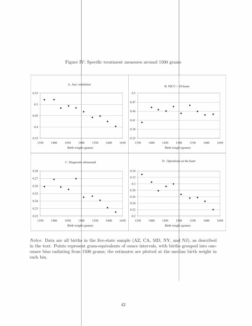
Figure IV: Specific treatment measures around 1500 grams

C. Diagnostic ultrasound

0.22

0.23

0.24

0.25

0.26

0.27

0.28

1350 1400 1450 1500 1550 1600 1650

Birth weight (grams)

D. Operations on the heart

0.2

0.22

0.24

0.26

0.28

0.3

0.32

0.34

1350 1400 1450 1500 1550 1600 1650

Birth weight (grams)

A. Any ventilation

0.35

0.4

0.45

0.5

0.55

1350 1400 1450 1500 1550 1600 1650

Birth weight (grams)

B. NICU > 24 hours

0.35

0.38

0.41

0.44

0.47

0.5

1350 1400 1450 1500 1550 1600 1650

Birth weight (grams)

Notes: Data are all births in the five-state sample (AZ, CA, MD, NY, and NJ), as describedin the text. Points represent gram-equivalents of ounce intervals, with births grouped into one-ounce bins radiating from 1500 grams; the estimates are plotted at the median birth weight ineach bin.

42

Figure V: Covariates around 1500 grams

A: Gestational age

31

31.4

31.8

32.2

32.6

33

1350 1400 1450 1500 1550 1600 1650

Birth weight (grams)

B: Mother's age

26

26.2

26.4

26.6

26.8

27

1350 1400 1450 1500 1550 1600 1650

Birth weight (grams)

C: Mother's education: Less than high school

0.24

0.245

0.25

0.255

0.26

0.265

0.27

1350 1400 1450 1500 1550 1600 1650

Birth weight (grams)

D: Mother's race: White

0.42

0.43

0.44

0.45

0.46

1350 1400 1450 1500 1550 1600 1650

Birth weight (grams)

E: Singleton birth

0.72

0.74

0.76

0.78

1350 1400 1450 1500 1550 1600 1650

Birth weight (grams)

F: Vaginal delivery

0.42

0.44

0.46

0.48

0.5

0.52

1350 1400 1450 1500 1550 1600 1650

Birth weight (grams)

I: Year of birth

1992

1992.5

1993

1993.5

1994

1350 1400 1450 1500 1550 1600 1650

Birth weight (grams)

J: Predicted one-year mortality

0.04

0.05

0.06

0.07

0.08

1350 1400 1450 1500 1550 1600 1650

Birth weight (grams)

G: Fewer than 7 prenatal visits

0.25

0.28

0.31

0.34

0.37

0.4

1350 1400 1450 1500 1550 1600 1650

Birth weight (grams)

H: Tocolysis

0.1

0.11

0.12

0.13

1350 1400 1450 1500 1550 1600 1650

Birth weight (grams)

Notes: NCHS birth cohort linked birth/infant death files, 1983-1991 and 1995-2003, as describedin the text. Points represent gram-equivalents of ounce intervals, with births grouped into one-ounce bins radiating from 1500 grams; the estimates are plotted at the median birth weight ineach bin.

43

Figure VI: First stage versus reduced form, by NICU quality level

-0.90

-0.80

-0.70

-0.60

-0.50

-0.40

-0.30

-0.20

-0.10

0.00

0.10

0.20

0.30

0.40

-0.15 -0.10 -0.05 0.00 0.05 0.10 0.15 0.20 0.25 0.30 0.35 0.40 0.45 0.50 0.55 0.60 0.65 0.70

hospital charges [2006$]: (coefficient / mean above threshold)

on

e-y

ear

mo

rtality

: (c

oeff

icie

nt

/ m

ean

ab

ove t

hre

sh

old

)

Level 0/1/2 NICU

no NICU

Level 3B NICU

Level 3A NICU

Level 3C NICU

Level 3D NICU

Notes: Plot of first stage coefficients (for 2006 charges, in levels) and reduced form coefficients(for one-year mortality) by NICU level in our California data. See text for details on the NICUclassifications.

44

Supplementary online appendix

1

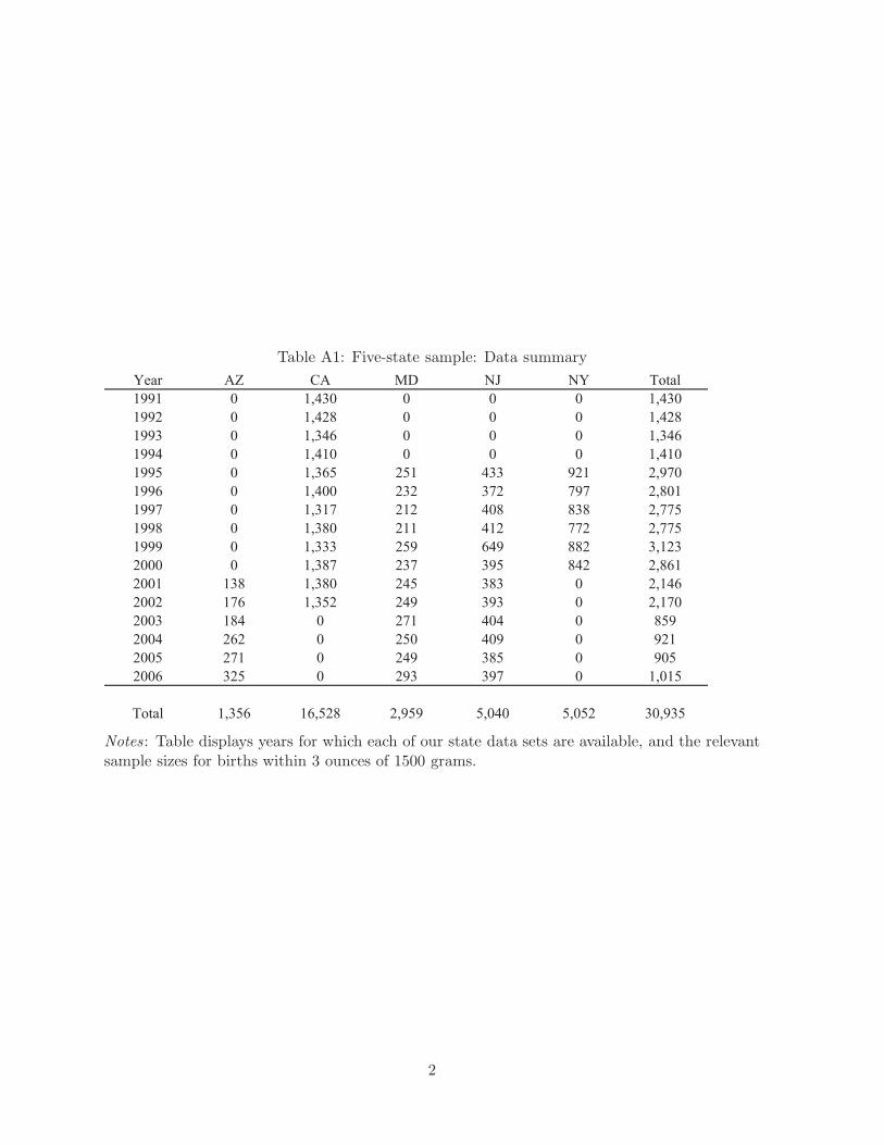
Table A1: Five-state sample: Data summary

Year AZ CA MD NJ NY Total

1991 0 1,430 0 0 0 1,430

1992 0 1,428 0 0 0 1,428

1993 0 1,346 0 0 0 1,346

1994 0 1,410 0 0 0 1,410

1995 0 1,365 251 433 921 2,970

1996 0 1,400 232 372 797 2,801

1997 0 1,317 212 408 838 2,775

1998 0 1,380 211 412 772 2,775

1999 0 1,333 259 649 882 3,123

2000 0 1,387 237 395 842 2,861

2001 138 1,380 245 383 0 2,146

2002 176 1,352 249 393 0 2,170

2003 184 0 271 404 0 859

2004 262 0 250 409 0 921

2005 271 0 249 385 0 905

2006 325 0 293 397 0 1,015

Total 1,356 16,528 2,959 5,040 5,052 30,935

Notes: Table displays years for which each of our state data sets are available, and the relevantsample sizes for births within 3 ounces of 1500 grams.

2

Table A2: Selected covariate comparison (controlling for trends in birth weight)

adjusted mean raw mean

below threshold above threshold p-value1

p-value2

(1) (2) (3) (4)

Fewer than 7 Prenatal visits 0.3212 0.3172 (0.310) (0.702)

First birth 0.4109 0.4149 (0.418) (0.503)

Mother's Age 26.67 26.43 (0.000)** (0.339)

Mother's Education: <High School 0.2473 0.2503 (0.518) (0.577)

Mother's Education: High School 0.3338 0.3358 (0.710) (0.876)

Mother's Education: Some College 0.1784 0.1734 (0.132) (0.239)

Mother's Education: College+ 0.1521 0.1501 (0.489) (0.769)

Mother's Education: Missing 0.0875 0.0905 (0.204) (0.721)

Mother born outside state 0.4139 0.4079 (0.166) (0.650)

Mother's Race: White 0.4483 0.4493 (0.773) (0.920)

Mother's Race: African American 0.2549 0.2539 (0.816) (0.906)

Mother's Race: Hispanic 0.1399 0.1279 (0.000)** (0.537)

Father's Age 30.03 29.87 (0.037)* (0.440)

Missing Father's Age 0.2390 0.2434 (0.267) (0.549)

Father's Education: <High School 0.1284 0.1274 (0.813) (0.834)

Father's Education: High School 0.2642 0.2652 (0.854) (0.927)

Father's Education: Some College 0.0997 0.0987 (0.811) (0.806)

Father's Education: College+ 0.1051 0.1071 (0.672) (0.689)

Father's Education: Missing 0.4026 0.4016 (0.901) (0.953)

Male 0.5004 0.5024 (0.720) (0.752)

Gestational Age 32.29 32.47 (0.000)** (0.003)**

Singleton Birth 0.7372 0.7452 (0.054) (0.316)

Twin Birth 0.2229 0.2189 (0.236) (0.298)

Multiple (non-twin) Birth 0.0389 0.0359 (0.060) (0.439)

Vaginal Birth 0.4582 0.4662 (0.147) (0.267)

Obstetric Procedures: Amnioscentesis 0.0520 0.0510 (0.616) (0.762)

Obstetric Procedures: Induction 0.1048 0.0978 (0.037)* (0.381)

Obstetric Procedures: Stimulation 0.0682 0.0642 (0.125) (0.387)

Obstetric Procedures: Tocolysis 0.1296 0.1166 (0.000)** (0.298)

Obstetric Procedures: Ultrasound 0.6607 0.6497 (0.035)* (0.369)

Obstetric Procedures: Other 0.0690 0.0630 (0.022)* (0.641)

Year of Birth 1993.61 1993.03 (0.000)** (0.409)

Predicted 1-year Mortality 0.0551 0.0575 (0.000)** (0.391)

Notes: Data is NCHS birth cohort linked birth/infant death files, 1983-1991 and 1995-2003,as described in the text. For most covariates, the number of observations is 341,140. De-livery method is available for 229,843 births; obstretric procedures are available for 229,175births. * significant at 5%; ** significant at 1%. Column (3) reports p-values calculated fromheteroskedastic-robust standard errors; column (4) reports p-values calculated from standarderrors clustered at the gram level.

3

Table A3: Bandwidth sensitivity

A. NCHS Nationwide Data

Dependent variable:

1-year

Mortality

Bandwidth 30 60 90 120 150

Birth weight < 1500g -0.0267 -0.0162 -0.0114 -0.00911 -0.00865

(0.00382)** (0.00269)** (0.0022)** (0.00190)** (0.00170)**

Mean of dependent variable above cutoff: 0.0607 0.0562 0.0545 0.0532 0.0515

Observations 72937 163415 233880 304630 376400

Dependent variable:

28-Day

Mortality

Bandwidth 30 60 90 120 150

Birth weight < 1500g -0.0228 -0.0146 -0.0101 -0.00828 -0.00773

(0.00322)** (0.00227)** (0.00185)** (0.00160)** (0.00143)**

Mean of dependent variable above cutoff: 0.0431 0.0390 0.0377 0.0367 0.0352

Observations 72937 163415 233880 304630 376400

B. 5-State Sample

Dependent variable:

Hospital

Charges

Bandwidth 30 60 90 120 150

Birth weight < 1500g 7670 8380 9290 8070 6490

(4300)* (3210)** (2630)** (2270)** (2030)**

Mean of dependent variable above cutoff: 83890 81527 80235 79092 77158

Observations 10533 21404 31990 42012 52471

Dependent variable:

Hospital

Costs

Bandwidth 30 60 90 120 150

Birth weight < 1500g 4460 3620 3970 3410 2580

(1880)* (1390)** (1140)** (985)** (881)**

Mean of dependent variable above cutoff: 41063 39321 38572 38028 37094

Observations 10533 21404 31990 42012 52471

Dependent variable:

Length of

Stay

Bandwidth 30 60 90 120 150

Birth weight < 1500g 2.38 1.84 1.91 1.53 1.14

(0.743)** (0.536)** (0.439)** (0.379)** (0.340)**

Mean of dependent variable above cutoff: 25.7 24.8 24.3 24.0 23.5

Observations 11254 22877 34183 44868 56067

Notes: All models are local linear regressions, estimated on the specified bandwidth of grams above and below VLBW threshold. All modelsinclude linear gram-trend variables and our “main controls,” which vary by the sample used and are described in the notes in the previoustables. Some observations have missing charges, as described in the text. * significant at 5%; ** significant at 1%. Heteroskedastic-robuststandard errors in parentheses.

4

Table A4: Polynomial order sensitivity

A. NCHS Nationwide Data

Dependent variable:

1-year

Mortality

Polynomial of order: 1 2 3 4

-0.0072 -0.0103 -0.0143 -0.0144

Birth weight < 1500g (0.0022)** (0.0038)** (0.0062)* (0.0082)

[0.0040] [0.0067] [0.0099] [0.0122]

Mean of dependent variable above cutoff: 0.0553

Observations 202071

B. 5-State Sample

Dependent variable:

Hospital

Charges

Polynomial of order: 1 2 3 4

Birth weight < 1500g 9,065 4,809 2,350 6,688

(2,297)** (3,363) (4,442) (5,879)

[5,094] [7,099] [9,325] [12,508]

Mean of dependent variable above cutoff: 81566

Observations 28928

Notes: All models are OLS, estimated on a sample within 3 ounces above and below VLBW threshold. All models include the gram-trendvariables of the stated polynomial order and our “main controls,” which vary by the sample used and are described in the notes in the previoustables. Some observations have missing charges, as described in the text. * significant at 5%; ** significant at 1%. Heteroskedastic-robuststandard errors in parentheses; standard errors clustered at the gram level in brackets.

5

Table A5: Coefficients on selected covariates

Sample: NCHS Nationwide Data Multi-State Sample

Dependent variable: 1-year mortality hospital charges

Birth weight < 1500g -0.0072 Birth weight < 1500g 9,065

(0.0022)** (2,297)**

Birth weight < 1500g * Grams from cutoff (100s) -0.0111 Birth weight < 1500g * Grams from cutoff (100s) 617

(0.0032)** (3,463)

Birth weight >= 1500g * Grams from cutoff (100s) -0.0184 Birth weight >= 1500g * Grams from cutoff (100s) -7,951

(0.0029)** (2,823)**

Prenatal Visits: 7-10 -0.0063 =1 if newborn is male and not missing 11,611

(0.0014)** (1,145)**

Prenatal Visits: >=11 -0.0065 Pre-term birth 22,958

(0.0015)** (1,688)**

Mother born outside state -0.0012 Mother's Race/Ethnicity: African American 1,827

(0.0011) (1,481)

First Birth 0.0191 Mother's Race/Ethnicity: Other 4,533

(0.0012)** (1,600)**

Mother's Age: 31-35 (compared to <16) -0.0129 Twin birth 3,405

(0.0049)** (1,346)*

Mother's Age: 36-40 -0.0118 Multiple (non-twin) birth 11,835

(0.0051)* (2,354)**

Mother's Age: 41+ -0.0007 Cesarean Section 2,770

(0.0065) (1,199)*

Mother's Education: High School 0.0004 Arizona (compared to MD) -1,653

(0.0015) (2,484)

Mother's Education: Some College -0.0025 California 101,580

(0.0017) (1,805)**

Mother's Education: College+ 0.0037 New Jersey 87,235

(0.0019) (1,608)**

Moher's Education: missing 0.0177 New York 60,591

(0.0028)** (1,500)**

Father's Age: 31-35 (compared to <16) -0.0009 Year = 1991 (compared to 2003) -92,968

(0.0188) (4,690)**

Father's Age: 36-40 -0.0012 Year = 2006 3,937

(0.0188) (4,694)

Father's Age: 41+ -0.0041 Constant 31,557

(0.0188) (4,237)**

Father's Age: missing 0.0020

(0.0187)

Male 0.0144

(0.0010)**

Gestational Age: 37 weeks (compared to <31) 0.0256

(0.0038)**

Gestational Age: 40 weeks 0.0124

(0.0053)*

Gestational Age: 42+ weeks 0.0081

(0.0052)

Mother's Race/Ethnicity: African American -0.0191

(0.0014)**

Mother's Race/Ethnicity: Hispanic -0.0035

(0.0019)

Singleton birth 0.0442

(0.0018)**

Twin birth 0.0113

(0.0017)**

Year = 2002 (compared to 1984) -0.0354

(0.0035)**

Constant 0.0489

(0.0243)*

Mean of dependent variable above cutoff: 0.0553 81566

Observations 202071 28928

Notes: All models are OLS, estimated on a sample within 3 ounces above and below VLBWthreshold. Charges are in $2006. Some observations have missing charges, as described in thetext. We only show a sub-set of the coefficients on these covariates in order to keep the table toone page. Five states include AZ, CA, MD, NY, and NJ (various years) * significant at 5%; **significant at 1%. Heteroskedastic-robust standard errors in parentheses.

6

Table A6: Alternative first stage outcomeslog median regression

Dependent variable: hospital costs hospital costs log(hospital costs) (hospital charges) hospital charges log(length of stay)

Birth weight < 1500g 4189 3795 0.263 0.263 9415 0.140

(1066)** (1030) (0.106)** (0.035)** (1593)** (0.0272)**

[2610] [2399] [0.1060]* [0.1059]* CI: [1485, 21526]** [0.0713]

Sample 5-State 5-State 5-State 5-State 5-State 5-State

Controls No Yes Yes Yes Yes Yes

Mean of dependent variable above cutoff: 39410 39410 9.91 10.58 81566 2.78

Observations 28928 28928 28769 28769 28928 30935

hospital hospital charges hospital costs log(charges) log(length of stay)

Dependent variable: transfer including transfers including transfers including transfers including transfers

Birth weight < 1500g -0.011 7297 2872 0.223 0.1088

(0.0067) (4313) (1776) (0.045)** (0.0319)**

[0.0128] [6,021] [2,529] [0.0707]** [0.0388]**

Sample 5-State California California California California

Controls Yes Yes Yes Yes Yes

Mean of dependent variable above cutoff: 0.100 109421 45141 11.0 2.99

Observations 30935 14560 14560 14560 16528

Notes: All models are OLS except the median regression, and all are estimated on a sample within 3 ounces above and below VLBWthreshold. All models include the gram-trend variables and our “main controls,” which are listed in Table A5, as well as indicators for eachyear. Charges are in 2006 dollars. Some observations have missing or zero charges, as described in the text. Five states include AZ, CA,MD, NY, and NJ (various years). * significant at 5%; ** significant at 1%. Heteroskedastic-robust standard errors in parentheses; standarderrors clustered at the gram level in brackets. The 95% confidence interval reported for the median regression was bootstrapped, with 500samples clustered by birth weight.

7

Table A7: Results by year and for overlap of NCHS/five-state data

A. NCHS Nationwide Data

Five states,

Dependent variable: Five states, years in NCHS

all NCHS years and multi-state data

1983-1987 1988-1991 1995-1998 1999-2002 1983-2002 1991; 1995-2002

(available years)

Birth weight < 1500g -0.0144 -0.0076 -0.0006 -0.0070 -0.0104 -0.0074

(0.0051)** (0.0048) (0.0038) (0.0035)* (0.0042) (0.0051)

[0.0052]** [0.0063] [0.0056] [0.0037] [0.0077] [0.0063]

Mean of dependent variable above cutoff: 0.0813 0.0622 0.0410 0.0378 0.054 0.039

Observations 50947 47545 49989 53590 49399 23698

B. Multi-State Sample

Dependent variable: hospital charges hospital charges hospital charges hospital charges hospital charges hospital costs

1991-1994 1995-1998 1999-2002 2003-2006 1991; 1995-2002 1991; 1995-2002

Birth weight < 1500g 12055.25 3514.89 16985.481 582.315 10108 4553

(4,538)** (3,167) (4,930)** (6,151) (2738)** (1242)**

[4,799]* [5,426] [7,998]* [7,149] [5,947] [2,791]

Mean of dependent variable above cutoff: 69566 71392 93717 96124 80721 39946

Observations 5018 10711 9504 3695 21479 21479

In-hospital births only

In-hospital births only

Years:

Years:

Years in NCHS

and multi-state data

1-year mortality

Notes: All models are OLS, estimated on a sample within 3 ounces above and below VLBW threshold. All models include the gram-trendvariables. The first four columns include our “main controls,” which vary by the sample used and are described in the notes in the previoustables. The last two columns include common covariates across samples: indicators for whether the baby is male, preterm, black,“other”race, a twin, or a non-twin multiple birth, as well as state indicators and year indicators. Although in theory the births included in theNCHS birth records in the state-years available in our multi-state sample should be the same as the births included in the multi-statesample, in practice the samples are slightly different (as evidenced by the difference in sample size), largely due to 300-400 fewer births inthe discharge data in each year from 2000-2002. Some observations have missing charges, as described in the text. * significant at 5%; **significant at 1%. Robust standard errors in parentheses.

8

Table A8: One-year mortality results by cause of death

Dependent variable:

infectious and

parasitic

diseases neoplasms

endocrine,

nutritional,

metabolic,

immunity,

blood disorders

nervous

system, sense

organ disorders

respiratory

system

disorders

digestive

system

disorders

congenital

anomalies

perinatal

conditions

symptoms,

signs, ill-

defined

conditions other

Model: OLS OLS OLS OLS OLS OLS OLS OLS OLS OLS

Birth weight < 1500g -0.0026 0.0009 0.0024 -0.0141 0.0015 -0.0003 0.0022 -0.0206 0.0185 0.0121

(0.0055) (0.0025) (0.0031) (0.0050)** (0.0071) (0.0051) (0.0178) (0.0179) (0.0107) (0.0093)

[0.0061] [0.0018] [0.0028] [0.0041]** [0.0057] [0.0035] [0.0102] [0.0156] [0.0084]* [0.0060]*

Trend controls Yes Yes Yes Yes Yes Yes Yes Yes Yes Yes

Year controls Yes Yes Yes Yes Yes Yes Yes Yes Yes Yes

Main controls Yes Yes Yes Yes Yes Yes Yes Yes Yes Yes

Mean of dependent variable above cutoff: 0.0222 0.0034 0.0050 0.0199 0.0334 0.0151 0.4164 0.3410 0.0850 0.0585

Dependent variable:

"external"

cause

respiratory

distress

syndrome

(RDS)

sudden infant

death

syndrome

(SIDS) jaundice meningitis

Model: OLS OLS OLS OLS OLS

Birth weight < 1500g 0.0042 0.0008 0.0166 -0.0030 -0.0021

(0.0048) (0.0106) (0.0093) (0.0018) (0.0030)

[0.0034] [0.0085] [0.0068]* [0.0011]** [0.0036]

Trend controls Yes Yes Yes Yes Yes

Year controls Yes Yes Yes Yes Yes

Main controls Yes Yes Yes Yes Yes

Mean of dependent variable above cutoff: 0.0139 0.0802 0.0617 0.0025 0.0050

Observations 11090

one-year mortality, partitioned by broad cause-of-death categories

one-year mortality, by selected individual causes of death (not a partition)

Notes: This table presents results by cause of death among infants who died within one year of birth (that is, the sample is not all infantsbut rather all infants who died within one year of birth). The ten cause of death classifications (other than all cause mortality) in the firstrow were constructed to be categories which could be defined consistently over time, across a change in cause of death coding which occurspartway through our sample; these broad categories partition non-missing causes of death. The second row extracts some individual causesof death from these broad categories. We exclude observations with missing information on the timing or cause of death. OLS modelsestimated on a sample within 3 ounces above and below the VLBW threshold. All models include the gram-trend variables. * significantat 5%; ** significant at 1%. Heteroskedastic-robust standard errors in parentheses; standard errors clustered at the gram level in brackets.

9

Figure A1: Birth frequencies for wider bandwidths

A: Birth frequency by gram

0

200000

400000

600000

800000

1000000

1200000

1400000

250 875 1500 2125 2750 3375 4000 4625 5250 5905 7350

Birth weight (grams)

B: Birth frequency by gram: 1000-2500 grams

0

50000

100000

150000

200000

250000

1000 1200 1400 1600 1800 2000 2200 2400

Birth weight (grams)

Notes: NCHS birth cohort linked birth/infant death files, 1983-1991 and 1995-2003, as described in the text.

10

Figure A2: Alternative first stage outcomes

A: 5-State: Median charges

45000

50000

55000

60000

65000

70000

75000

1350 1400 1450 1500 1550 1600 1650

Birth weight (grams)

B: California: Median charges, incl. transfers

55000

65000

75000

85000

95000

1350 1400 1450 1500 1550 1600 1650

Birth weight (grams)

C: 5-State: log(charges)

10.4

10.5

10.6

10.7

10.8

10.9

1350 1400 1450 1500 1550 1600 1650

Birth weight (grams)

D: California: log(charges, incl. transfers)

10.9

11

11.1

11.2

11.3

1350 1400 1450 1500 1550 1600 1650

Birth weight (grams)

E: 5-State: Median log(charges)

10.8

10.9

11

11.1

11.2

11.3

1350 1400 1450 1500 1550 1600 1650

Birth weight (grams)

F: California: Median log(charges incl. transfers)

11

11.1

11.2

11.3

11.4

11.5

11.6

1350 1400 1450 1500 1550 1600 1650

Birth weight (grams)

Notes: Data are all births in the five-state sample (AZ, CA, MD, NY, and NJ), as describedin the text. Some observations have missing or zero charges, as described in the text. Chargesare in 2006 dollars. Points represent gram-equivalents of ounce intervals, with births groupedinto one-ounce bins radiating from 1500 grams; the estimates are plotted at the median birthweight in each bin. Discussion: The upward slope for log charges in Panel C is largely drivenby newborns with few charges. The upward slope disappears when the sample is restricted tonewborns with greater the $3,000 in charges. A plot of an indicator that the newborn accruedcharges of less than $3,000 against birth weight revealed a fairly noisy series. Further, when datafrom hospitals where newborns were transferred are included using the longitudinal data fromCalifornia (panel D), log charges are relatively flat at 11.17 in the one-ounce bins just beforethe threshold and drop to 11.00 after the threshold. Panels E and F report similar estimatesto the main results when median log charges are compared in both the five-state sample and inthe California sample.

11