estimating regression models in which the dependent ... · estimating regression models in which...

Advance Access publication August 11, 2005 Political Analysis (2005) 13:345–364doi:10.1093/pan/mpi026

Estimating Regression Models in Which the DependentVariable Is Based on Estimates

Jeffrey B. Lewis and Drew A. LinzerDepartment of Political Science, University of California,Los Angeles, 4289 Bunche Hall, Los Angeles, CA 90095

e-mail: [email protected] (corresponding author)e-mail: [email protected]

Researchers often use as dependent variables quantities estimated from auxiliary data sets.

Estimated dependent variable (EDV) models arise, for example, in studies where counties

or states are the units of analysis and the dependent variable is an estimated mean,

proportion, or regression coefficient. Scholars fitting EDV models have generally recognized

that variation in the sampling variance of the observations on the dependent variable will

induce heteroscedasticity. We show that the most common approach to this problem,

weighted least squares, will usually lead to inefficient estimates and underestimated

standard errors. In many cases, OLS with White’s or Efron heteroscedastic consistent

standard errors yields better results. We also suggest two simple alternative FGLS

approaches that are more efficient and yield consistent standard error estimates. Finally,

we apply the various alternative estimators to a replication of Cohen’s (2004) cross-national

study of presidential approval.

1 Introduction

It is not uncommon for regressions to be run in which observations on the dependent

variable are estimated in an auxiliary analysis. For example, such dependent variables may

be calculated as sample means, vectors of regression coefficients, poll question marginals,

election vote shares, legislative seat shares, or fractions of bills vetoed; all such variables

are ‘‘estimated’’ in the sense that they are aggregated outcomes of individual-level data

generating processes. The fitting of such estimated dependent variable (EDV) regressions

is the subject of this paper.

In general, EDV regression models are the second stage in a two-stage estimation

process. The first stage uses observed data to estimate the values of the dependent variable;

the EDV model then regresses these values against one or more independent variables to

generate the ultimate coefficients of interest. An obvious context in which EDV regression

can arise is multilevel modeling.1 To foreshadow our application of an EDV model later in

this article, consider a simple two-level model in which the individual-level effect of

Authors’ note: We thank Chris Achen, Barry Burden, Michael Herron, Gary King, Eduardo Leoni, and LynnVavreck for comments on earlier drafts of this article. Any remaining errors are ours alone.1Guidance on multilevel models is often derived from such well-cited sources as Steenbergen and Jones (2002)and Bryk and Raudenbush (1992).

� The Author 2005. Published by Oxford University Press on behalf of the Society for Political Methodology.All rights reserved. For Permissions, please email: [email protected]

345

evaluations of the economy on leader approval (bottom level) is assumed to be a function

of state-level factors plus a random shock (top level). In this manner, a researcher can

investigate sources of cross-national causal heterogeneity and address questions of whysome independent variable may have a different effect on the dependent variable in

different countries.

Aside from a loss of efficiency, the fact that the dependent variable is estimated does

not necessarily present any difficulties for regression analysis. Indeed, such errors of

measurement are often explicitly included in discussions of regression residuals presented

in introductory textbooks (Maddala 2001, p. 64). However, if the sampling uncertainty in

the dependent variable is not constant across observations, the regression errors will be

heteroscedastic and ordinary least squares (OLS) will introduce further inefficiency and

may produce inconsistent standard error estimates.

When the dependent variable in a regression is based on estimates, the regression

residual can be thought of as having two components. The first component is sampling

error (the difference between the true value of the dependent variable and its estimated

value). The second component is the random shock that would have obtained even if the

dependent variable were directly observed as opposed to estimated. The first component

will be heteroscedastic if the sampling variance differs across observations.2 But the

second component could well be homoscedastic. The usual approaches to EDV regression

are either to run OLS ignoring heteroscedasticity resulting from the first component of the

residual or to run a weighted least squares (WLS) model assuming that the entire residual,

and not just the first component, is heteroscedastic. Under this assumption, however, the

WLS approach, like the OLS approach, is also inefficient and may produce inconsistent

estimates of parameter uncertainty.

Our main finding for researchers interested in the application of EDV regression models

is that only when the share of the regression residual due to sampling error in the

dependent variable is very high (roughly 80% to 90% or more) does the standard WLS, in

which the observations are weighted by the inverse of the standard errors of the dependent

variable estimates, produce more efficient estimates than OLS. That is to say, the ‘‘cure’’

provided by the standard WLS is typically going to do more harm than good. Through

a series of Monte Carlo experiments, we find that when the sampling uncertainty

component is small relative to the total variation in the dependent variable and when this

uncertainty does not vary greatly from observation to observation, White’s (1980), and for

smaller samples, Efron heteroscedastic consistent standard error estimates yield good

results.3 If sampling error comprises a larger share of the variation in the dependent

variable and this uncertainty varies greatly across observations, appreciable gains in

efficiency can be achieved through the use of either of a pair of alternative feasible

generalized least squares (FGLS) estimators that we describe below.

The article is organized as follows. Section 2 reviews applications of models using

estimated dependent variables. Section 3 formalizes the problem of regressions involving

2For example, reported average state income may be based on a much larger sample in California than it is inRhode Island, leading California’s mean income to be more precisely estimated than Rhode Island’s. Somesurveys, such as the 1988 Senate Election Study, intentionally draw samples of roughly equal size from eachaggregate unit, thus avoiding much of the heteroscedasticity that is generally present when sample means areused as a dependent variable. In these cases, the heteroscedasticity from sampling error would only enter frominter-unit heterogeneity in the intra-unit variance of the variable being sampled.

3Efron standard errors (also known as HC3 standard errors) are based upon the jackknife techniques of Efron(1982) and are typically more accurate (as well as more conservative) than Huber-White standard errors insamples smaller than 250 observations; see Long and Ervin (2000) and MacKinnon and White (1985).

346 Jeffrey B. Lewis and Drew A. Linzer

estimated dependent variables. In Section 4 we compare the estimation of EDV models

with OLS or WLS to two FGLS estimators that allow the analyst to address the problem of

heteroscedasticity in the first-level error component without assuming that the second-

level error component is similarly heteroscedastic. The first FGLS approach assumes that

the sampling variances of the observations on the dependent variable are known, as would

be the case if, for example, the data were regression estimates or aggregated survey

responses. The second estimator requires only that the sampling errors be known up to

a proportional factor, as would be the case if the data were means based on samples of

differing sizes.4 Section 5 describes the Monte Carlo experiments. Section 6 presents an

empirical example based on the cross-national public opinion study by Cohen (2004).

Section 7 concludes.

2 Applications of EDV Models

Multilevel models may be estimated in several ways: (1) The parameters of each of the

levels can be estimated simultaneously; (2) Regressions can be run with a large number of

interaction terms between within- and across-country variables on the right hand side; or

(3) Two-stage approaches of the sort we consider here can be applied (for examples of the

first two approaches, see Lubbers et al. 2002; Anderson and Tverdova 2003; Banducci

et al. 2003; Peffley and Rohrschneider 2003; and Rohrschneider and Whitefield 2004).

Reviewing these alternatives, the ‘‘interaction term’’ model is generally not advised

because it assumes, almost certainly incorrectly, that there would be no residual in

a regression of individual-level coefficients on the country-level variables. Simultaneous

(or single-stage) estimation may take the form of a linear hierarchial model, for example.

Under a two-stage approach, the bottom-level parameters are first estimated within each

unit; then, in a second stage, an EDV regression is run in which the estimated quantities

from the first stage are used as dependent variables. An example of this multilevel, two-

stage modeling strategy can be found in Guerin et al. (2001), who examine determinants of

recycling behavior in 15 EU countries using survey data from the Eurobarometer: ‘‘The

first step was to estimate the person-level model. Then, we set up our model to predict the

variation of the coefficients b0j by introducing explanatory variables at the country level’’

(p. 204). Here, it is regression coefficients as estimates of the relationship at the micro level

that become the dependent variable in the top-level cross-national analysis.

The first-stage estimates that become the dependent variable in the second stage need

not be regression coefficients—indeed, they may be as simple as aggregate public opinion

poll marginals. One such study, which we shall replicate and extend below, is Cohen

(2004). He examines country-level approval of the chief executive as a function of each

country’s aggregate perceptions of the national economy in 41 countries, with survey

sample sizes ranging from 500 to 2189. Because both the estimates and the sample sizes

differ by country, the standard errors of the country-level dependent variable estimates will

also vary by country. Kaltenthaler and Anderson’s (2001) cross-national study of the

determinants of aggregate public support for the common European currency is a similar

example of using survey marginals as a dependent variable. It is also common to encounter

regressions using poll question marginals (such as presidential approval) as dependent

4In this case, if the within-unit variance of the variable were constant, the sampling variances would beproportional to 1/ni where ni is the size of the sample from which the mean was calculated for observation i.

347Estimated Dependent Variable Regressions

variables in opinion research that is not cross-national (Taylor 1980; MacKuen et al. 1989;

MacKuen et al. 1992; Oppenheimer 1996).5

While Hanushek (1974) and Jusko and Shively (2005) show that such two-stage

approaches can be efficient under certain circumstances and assumptions, in general, there

are potential efficiency gains from estimating both the bottom- and top-level parameters in

a single stage. In cases in which the amount of information available to estimate the

bottom-level effects in each top-level unit is small (particularly relative to the number of

top-level units), there are potential gains from ‘‘borrowing strength’’ across units and

increasing efficiency through a single-stage estimation that justify their use.

On the other hand, in many political science examples, considerable information is

available about the bottom-level effects. In these cases, the gains from estimating both

levels in a single step can be modest. To see this, note that no single-step estimator can

generate more efficient estimates of the top-level parameters than could be achieved if the

bottom-level parameters were known. Taking the simplest example in which the sampling

uncertainty in the bottom-level quantities of interest are constant across all top-level units,

the standard errors in the second-stage EDV regression are increased by

100

ffiffiffiffiffiffiffiffiffiffiffiffiffiffiS

1� R2

rpercent over what they would be if the first-level parameters were known, where S is the

ratio of estimation variance to all other variance in the second-stage dependent variable

and R2 is the R2 of the second-stage regression that would obtain if the values of the

dependent variable were not based on estimates. In the empirical example presented in

Section 6 below, S is approximately 0.005 and R2 is approximately 0.5. Thus the upper

bound on the loss of efficiency that arises from running a second-stage EDV regression is

on the order of 10%. Gains from a single-stage estimation would be less than this

theoretical upper bound and could be much less. Under these circumstances, the added

effort of fitting a more complex single-stage linear hierarchial model would provide little

advantage relative to the simple two-stage EDV method.

3 Regressions with Estimated Dependent Variables

Consider the following regression model,

yi ¼ b1 þXkj¼2

bjxij þ �i ð1Þ

5This very short summary hardly scratches the surface of the breadth and depth of possible applications of EDVregression models. However, we do wish to highlight that with respect to EDVs generated using King’s (1997)EI algorithm, Herron and Shotts (2003) point out that using the so-called precinct-level EI estimates asdependent variables in second-stage regressions will lead to attenuated estimates and more generally calls intoquestion the validity of using precinct-level EI estimates in subsequent analysis. It should be noted thetechniques we present below are predicated on the assumption that the data used are free of the features describedby Herron and Shotts. In particular, we assume that the sampling or measurement error in the dependent variable(Y* � Y) is independent of the independent variables and error term (X and �) of the regression. Also, usingdistrict-level EI estimates (for example, estimates of black turnout at the Congressional district level made byapplying EI to precinct-level data in each district) need not involve the same ‘‘logical inconsistency’’ identifiedby Herron and Shotts.


for observations i ¼ 1, . . . , N. Assume that this regression model meets all of the usual

Gauss-Markov assumptions. However, yi is not observable. Rather we observe an

unbiased estimate yi* where

y*i ¼ yi þ ui ð2Þ

and E(ui) ¼ 0 and Var(ui) ¼ x2i (for i ¼ 1, . . . , N). ui is the sampling error in yi* and x2

i is

the variance of that sampling error. Assume that the estimate of the dependent variable for

each observation is independent of the others.6 In particular, assume Cov(ui, uh) ¼ 0 for all

i 6¼ h. Now consider the regression formed by substituting Eq. (2) into Eq. (1),

y*i ¼ b1 þXkj¼2

bjxij þ ui þ �i:

Writing vi ¼ �i þ ui, we have

y*i ¼ b1 þXkj¼2

bjxij þ vi: ð3Þ

Obviously, if xi 6¼ xh for some i and h, vi is heteroskedastic. In particular, letting

v ¼ (v1, v2, . . . , vN)9,

Eðvv9Þ ¼ X ¼

r2 þ x21 0 . . . 0

0 r2 þ x22 . . . 0

..

. ... . .

. ...

0 . . . . . . r2 þ x2N

2666437775 ð4Þ

where Var(�) ¼ r2. If r2 and x2i were both known, a WLS approach would yield best

linear estimators. That is, OLS estimation of

wiyi ¼ b1wi þXkj¼2

bjxijwi þ wivi

where

wi ¼1ffiffiffiffiffiffiffiffiffiffiffiffiffiffiffiffiffi

r2 þ x2i

p ð5Þ

yields efficient estimates of the regression parameters.

In real-world applications, we generally have only estimates of the x2i (i ¼ 1, . . . , N)

and no knowledge of r2. In the next section, we consider four feasible approaches to this

problem in cases in which knowledge of r2 and/or the x2’s is missing or incomplete.

4 Approaches to Fitting Estimated Dependent Variable Regressions

We will consider four approaches to estimating EDV regressions. The first two are the

most commonly applied: OLS (with or without White’s or Efron heteroscedastic consistent

standard errors) and WLS using weights based on the inverse of the standard errors of the

6The first FGLS approach described below is trivially extended to the case in which the estimates are notindependent.


dependent variable estimates. The third is an FGLS procedure first suggested in Hanushek

(1974) appropriate for cases in which estimates or the true sampling variances of the yi* areavailable (i.e., the x2’s are known). The fourth is also an FGLS procedure appropriate for

cases in which the sampling variances of the yi*’s are known only up to a constant of

proportionality. Both of these estimators are very easy to implement using standard

statistical packages.7

4.1 Estimation by Ordinary Least Squares

Given the assumptions made previously, it is well known that Eq. (3) can be consistently

estimated by OLS. However, in order for OLS to be efficient, xi must be constant across

all observations. That is, only if the sampling variances of the y* are constant (or zero) willvi be homoscedastic and OLS efficient.

In general, OLS will not be efficient and the usual standard error estimator is, in

general, inconsistent. Thus OLS estimates will be less precise than is optimal and, under

some conditions, will produce badly inconsistent standard error estimates. Not surpris-

ingly, if the degree of variation in x2i is small or if r2 is large relative to the x2’s, then

OLS will perform quite well. That is, if the appropriate set of weights (wi for i ¼ 1, . . . , N)are nearly constant across observations, OLS will be nearly efficient.

The inconsistent OLS standard errors can be corrected using the White (1980) or Efron

(1982) heteroscedastic consistent standard error estimator. As will be shown below, the

Efron robust standard error estimator will correctly measure the uncertainty in OLS even in

fairly small samples. However, the OLS estimator may be quite inefficient in some cases.

OLS is inefficient because the partial information about the nature of the heteroscedasticity

(that is, knowledge of x2i ’s) is not used.

4.2 Estimation by Weighted Least Squares

The most commonWLS approach to EDVmodels is simply to set wi¼ 1/xi (i¼ 1, . . . , N).Such weighting is recommended in Saxonhouse (1976) and King (1997, p. 290), among

other places. As shown in Eq. (5), this weighting scheme implicitly sets r2 ¼ 0. In other

words, when weighting by 1/x in an EDV model, researchers are attributing all of the errorin the total residual vi to the heteroscedastic sampling error (ui) and none to the

homoscedastic noise (�i). This is equivalent to assuming that the R2 in their regression

would be 1 (r2 ¼ 0) if they directly observed the true y’s as opposed to the estimated y*’s.Of course, the assumption that the regression R2 would be 1 if the true dependent

variable was directly observable will not typically be met. However, as will be shown in

the Monte Carlo simulation in the next section, if the variance of the homoscedastic noise

(r2) is very small in comparison to the variances of the sampling errors (the x2i ’s), the

assumption that r2 ¼ 0 may not be too costly. However, as r2 grows relative to the x2i ’s,

the WLS estimator becomes increasingly—and quite badly—inefficient and generates

highly misleading standard error estimates.8

Given only these two options, researchers face a trade-off. Use OLS with robust

standard error estimates and get possibly inefficient parameter estimates but good

estimates of the parameter uncertainty. Or use WLS and get possibly much more efficient

parameter estimates, but risk getting very misleading standard errors. Some scholars have,

7R functions implementing both of these procedures are available from the authors.8These conclusions are not specific only to the EDV case, but generalize to other cases in which WLS is appliedusing incorrect weights (see Greene 2003).


in fact, presented both estimates (Burden and Kimball 1998). This is a good practice.

However, when the methods yield estimates that differ in substantively significant ways,

simply reporting both sets of results is not entirely satisfying.

In the next two subsections, we will present two alternative estimation techniques that

are asymptotically efficient and whose standard errors are consistent regardless of the

relative size of r2 and the x2’s. Both of these estimators are FGLS estimators that use OLS

to generate consistent estimates of the v’s. These estimated v’s are used to find consistent

estimates of x2i þ r2 (for i ¼ 1, . . . , N) from which weights are created and a second-

stage WLS model fit.

4.3 Estimating x2 þ r2 when x2 is known

In this section, we present an FGLS estimator that is appropriate for cases in which the

standard errors of the estimated dependent variable are known, or at least where reliable

estimates are available. This method was first suggested by Hanushek (1974) for the case

in which the dependent variable is estimated regression coefficients. Since the x’s are

assumed to be known, only an estimate of r2 (the variance of the component of the

regression residual that is not due to sampling of the dependent variable) is required in

order to construct a proper set of weights to use in a second-stage WLS regression. To

arrive at an estimate of r2, first run OLS and calculate residuals vi for i ¼ 1, . . . , N.Following Hanushek (1974), the expectation of the sum of squared residuals from this

OLS regression can be written as

EXi

v2i

!¼ Eðv9vÞ � trððX9XÞ�1X9XXÞ;

where X is the variance covariance matrix of the vector of regression residuals v given in

Eq. (4) and tr(�) is the trace operator.9 E(v9v) ¼ E(P

i v2i ) and

EXi

v2i

!¼ E

Xi

ð�2i þ u2i þ 2�iuiÞ" #

¼ EXi

�2i

" #þ E

Xi

u2i

" #þ 0

¼ Nr2 þXi

x2i :

Writing X as r2I þ G where I is an n 3 n identity matrix and G is an n 3 n diagonal

matrix with x2i as the ith diagonal element, we have

EXi

v2i

!¼ Nr2 þ

Xi

x2i � trððX9XÞ�1X9ðr2IþGÞXÞ

¼ Nr2 þXi

x2i � r2trððX9XÞ�1X9XÞ � trððX9XÞ�1X9GXÞ

¼ ðN � kÞr2 þXi

x2i � trððX9XÞ�1X9GXÞ;

9The trace of a square matrix is the sum of its diagonal elements.


where k is the number of columns in X. Rearranging, we have

r2 ¼EP

i v2i

� ��P

i x2i þ trððX9XÞ�1X9GXÞN � k

;

implying that

r2 ¼P

i v2i �

Pi x

2i þ trððX9XÞ�1X9GXÞN � k

is an unbiased estimator for r2. In small samples, r2 may be estimated to be less than 0.

In these cases, r2 can be set equal to 0 (yielding the standard WLS approach to EDV

regression).

Given this estimator for r2, a set of weights wi (for i ¼ 1, . . . , N) can be constructed

such that

wi ¼1ffiffiffiffiffiffiffiffiffiffiffiffiffiffiffiffiffi

x2i þ r2

p :

The main regression is then refit using these weights. Estimates from this regression will

be asymptotically efficient.

4.4 Estimating x2 þ r2 when x2 is known to a constant multiplicative factor

Sometimes researchers encounter situations in which they may know only the x2’s up to

some unknown constant of proportionality. A common example here would be a dependent

variable based on sample means. That is, yi* ¼Pni

m¼1 Yim/ni. Often, in such cases, we knowthe size of the samples upon which the estimates are based, but we do not know the exact

sampling variances of the estimated means. If we assume that the variance of Yim is

constant for all i and j, then we have

x2i ¼

jni;

where j is the variance of Y and ni is the size of the sample upon which the ith sample

mean is based.10

10The usual WLS approach described above is often advocated for this case (Hanushek and Jackson 1977). Thejustification is as follows. Suppose that all the variables are measured as sample means. Then assume there is anunderlying individual-level regression model,

Yim ¼ b1 þXkj¼2

bkximj þ �im:

Assuming that �im is i.i.d. and taking means within each sampling unit i, we find,

y*i ¼ b1 þXkj¼2

bk�xij þ ��i;

where the variance of ��i will be proportional to ni (the number of individuals sampled in each unit i). In this case,weighting the entire regression residual by

ffiffiffiffini

pwould be appropriate. However, if some x’s that are uncorrelated

to � at both the individual and aggregate level are omitted, we will have an additional error component that is notheteroscedastic in proportion to 1/ni.


Again, we first run OLS and use the estimated residuals to form a set of weights,

wi (i ¼ 1, . . . , N) that can then be used in a second-stage WLS regression. We begin by

noting that the expectation of the true squared error terms is

Eðv2i Þ ¼ r2 þ jni:

If v ¼ (v1, . . . , vN)9 were observed directly, r2 and j could be estimated efficiently by the

OLS regression of v2 on (1/n). Since the v’s are consistent estimators for the v’s, we have

plimN!‘

Eðv2i Þ ¼ r2 þ j1

ni

� �:

One can then consistently estimate r2 and j by regressing v on (1/n). As above, this

method can yield estimates of r2 , 0. In these cases, the regression of v2 on (1/n) can be

rerun constraining the constant (r2) to be 0. Predicted values from the regression of v2 on(1/n) are estimates of r2 þ x2

i . Using these estimates, we next construct a set of weights

where

wi ¼1ffiffiffiffiffiffiffiffiffiffiffiffiffiffiffiffiffiffiffiffiffiffiffiffiffiffi

r2 þ jð1=niÞp :

The general procedure is as follows:

1. Regress y* on X by OLS and calculate the squared residuals v2i for i ¼ 1, . . . , N.

2. Regress v2 on ~x2i where ~x2

i is proportional to the variance of u (i.e. ~x2i ¼ x2

i /j).If the constant in this regression is negative (r2 , 0), the regression is rerun

constraining the constant to be 0. Calculate predicted values from this regression.

These predicted values are consistent estimates of x2i þ r2.

3. Fit the WLS regression of y* on X using weights wi ¼ 1ffiffiffiffiffiffiffiffiffiffiffiffir2þj~x2

i

p .

Because this method involves estimating not only r2, but also j, it will yield less-efficient

estimates than those that can be achieved if the x2’s are known exactly and only r2 must

be estimated.

5 Monte Carlo Analysis

In this section, we describe a series of Monte Carlo experiments that we conducted in order

to ascertain the small sample properties of each of the estimators for the EDV model

described above.

The regression model used for all the experiments is

yi ¼ 1þ 1xi þ vi;

where vi ¼ �i þ ui. Both � and u are drawn from independent (conditional) normal

distributions, �i ; N(0, x2i ) and ui ; N(0, 1 � C) for i ¼ 1, . . . , N. The x2’s are drawn

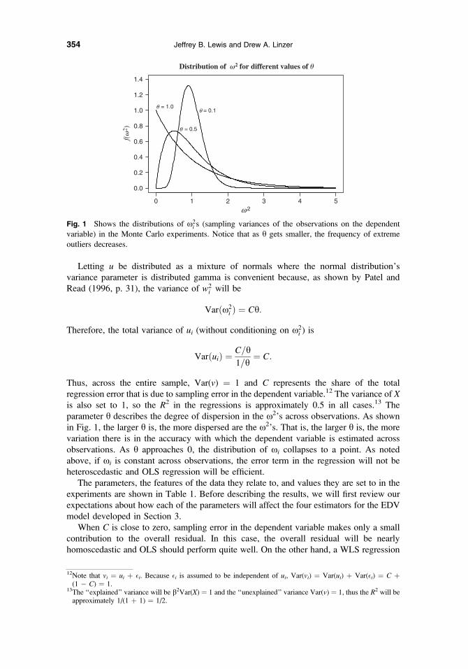
from a gamma distribution. In particular, x2i ; Gamma(C/h, 1/h).11

11The parameterization of the gamma distribution used here follows DeGroot and Schervish (2002). We definethe density of gamma distribution as f(z j a, b) ¼ [�(a)]�1baza�1e�bz for a . 0, b . 0, and z . 0. Given thisparameterization, E(Z) ¼ a/b and Var(Z) ¼ a/b2. In the simulations, the density of x2

i is f(x2i j C/h, 1/h).


Letting u be distributed as a mixture of normals where the normal distribution’s

variance parameter is distributed gamma is convenient because, as shown by Patel and

Read (1996, p. 31), the variance of w2i will be

Varðx2i Þ ¼ Ch:

Therefore, the total variance of ui (without conditioning on x2i ) is

VarðuiÞ ¼C=h1=h

¼ C:

Thus, across the entire sample, Var(v) ¼ 1 and C represents the share of the total

regression error that is due to sampling error in the dependent variable.12 The variance of Xis also set to 1, so the R2 in the regressions is approximately 0.5 in all cases.13 The

parameter h describes the degree of dispersion in the x2’s across observations. As shown

in Fig. 1, the larger h is, the more dispersed are the x2’s. That is, the larger h is, the more

variation there is in the accuracy with which the dependent variable is estimated across

observations. As h approaches 0, the distribution of xi collapses to a point. As noted

above, if xi is constant across observations, the error term in the regression will not be

heteroscedastic and OLS regression will be efficient.

The parameters, the features of the data they relate to, and values they are set to in the

experiments are shown in Table 1. Before describing the results, we will first review our

expectations about how each of the parameters will affect the four estimators for the EDV

model developed in Section 3.

When C is close to zero, sampling error in the dependent variable makes only a small

contribution to the overall residual. In this case, the overall residual will be nearly

homoscedastic and OLS should perform quite well. On the other hand, a WLS regression

Fig. 1 Shows the distributions of x2i s (sampling variances of the observations on the dependent

variable) in the Monte Carlo experiments. Notice that as h gets smaller, the frequency of extreme

outliers decreases.

12Note that vi ¼ ui þ �i. Because �i is assumed to be independent of ui, Var(vi) ¼ Var(ui) þ Var(�i) ¼ C þ(1 � C) ¼ 1.

13The ‘‘explained’’ variance will be b2Var(X) ¼ 1 and the ‘‘unexplained’’ variance Var(v) ¼ 1, thus the R2 will beapproximately 1/(1 þ 1) ¼ 1/2.


that weights by 1/x will ‘‘overcorrect’’ the heteroscedasticity that is generated by

estimation errors in the dependent variable. Thus, ceteris paribus, low values of C should

lead to poor WLS estimates.

The larger h is, the more heteroscedasticity is introduced by the sampling errors in the

dependent variable. When h is small, we expect that OLS will produce good estimates

because the regression error will exhibit little heteroscedasticity even if C is large.

However, if h is large, OLS is expected to be inefficient, particularly as C increases.

The value of q is mainly expected to affect the accuracy of the standard errors. It is

well known that OLS will produce inconsistent standard error estimates only if the

heteroscedasticity of the regression error depends on the independent variables in some way.

Thus we expect that OLS will be relatively efficient if q is small. However, as q grows, the

efficiency of the OLS estimates should decline and the standard error estimates worsen.

OLS combined with White’s (1980) standard errors should produce reasonable

estimates of model uncertainty for all parameter settings though the estimates may be

inefficient. The FGLS estimators should be efficient and produce good standard error

estimates for all parameter values.14

In all of the experiments described previously, we use data sets with 30 observations.

Similar results are obtained in experiments using data sets with greater numbers of obser-

vations. For each combination of the parameter values, 80,000 simulations were performed.

Table 2 shows the results for one particular set of parameters. In this experiment,

C ¼ 0.7, meaning that 70% of the variance in the residual is due to sampling error in the

dependent variable. The variation in the sampling error of the dependent variable across

observations is high (h ¼ 0.8). In particular, across the simulations the largest sampling

variance was about 200 times as large as the smallest on average. The correlation between

the sampling variances and the independent variable is set to 0.5.

All of the estimators yield estimates that are very accurate on average. Across the

simulated data sets, the average estimated regression slope was nearly identical (to four

decimal places) to the true value of b. This is not surprising, given that all the estimators

tested are known to be consistent, but it is comforting that they show little to no bias in

samples as small as 30. This is generally true for all of the combinations of parameter values

given in Table 1. Indeed, across all of the experiments that we conducted the mean b

Table 1 Parameters for the Monte Carlo experiments

Parameter Description Values

C Share of variation in the regression

error due to estimation error in the

dependent variable (0.1, 0.2, . . . , 1.0)h Degree of variation in dependent

variable sampling variances across

observations (0.2, 0.5, 0.8)

q Correlation between X and sampling

variances of the dependent variable (0.0, 0.5, 1.0)

N Number of observations 30

b Regression slope 1

Note. Table describes parameters that were manipulated in the Monte Carlo experiments and the values to which

they were set. For each combination of parameter values, 80,000 simulations were performed.

14Exceptions to this claim are C ¼ 0 and C ¼ 1, where OLS and WLS, respectively, would be efficient.


did not differ from the true b in a statistically significant way. One convenient consequence

of all the estimators showing little to no bias is that their observed root mean square errors

(RMSEs) are basically equivalent to their observed sampling standard deviations. Thus the

observed RMSEs can be compared to the mean estimated standard errors to assess the

degree to which each model accurately represents the uncertainty of its estimates.

While the parameter values used to generate the results in Table 2 would seem to

approximate the conditions under which the WLS approach would be effective, the

experimental results suggest otherwise. Even with very highly dispersed x2’s and most of

the residual resulting from sampling error in the dependent variable, OLS produced more

efficient estimates with more accurate standard errors than did the standard WLS. The

FGLS estimators are both about 10% more efficient than OLS; further experimentation

(not reported here) indicates that the efficiency gain from the FGLS models is even greater

in larger sample sizes. Additionally, both of these FGLS estimators produced accurate

standard error estimates in this experiment.

WLS produced highly misleading standard error estimates. While the standard deviation

of the WLS slope estimator across the repetitions was 0.228 (see the ‘‘RMSE’’ column in

the table), the average standard error estimate was 0.158. Thus, on average, the observed

standard deviation of the estimated b across the simulations was 144% greater than the

estimated standard errors. As we expected, OLS also produces inconsistent standard error

estimates. However, the observed OLS root mean square error was only 112% greater than

the mean estimated OLS standard error. White’s (1980) heteroscedastic consistent standard

error estimator actually does not improve the estimation of the standard error of b a great

deal in this example. However, accurate (albeit somewhat conservative) estimates of OLS

parameter uncertainty were obtained using Efron small-sample standard error estimates. As

noted earlier, as the size of the sample increases, White’s standard errors will increasingly

outperform the usual OLS standard errors as well as the Efron standard errors. Finally,

following our expectation, both of the FGLS estimators produced good estimates of

parameter uncertainty.

Table 2 Monte Carlo results for various EDV estimators

Method

Regression slope (b)

Mean

Observed rootmean squareerror (RMSE)

Mean estimatedstandard error (SE)

RMSE as apercentage ofmean est. SE

OLS

Usual SEs 1.00 0.211 0.188 112

White’s SEs 1.00 0.211 0.184 115

Efron SEs 1.00 0.211 0.214 98

WLS 1.00 0.228 0.158 144

FGLS

Known variance 1.00 0.189 0.174 109

Proportional variance 1.00 0.193 0.171 113

Note. Shows the results of one Monte Carlo experiment described in the text. The numbers reported in the

table are based on 200,000 simulations, with N ¼ 30 observations each. The parameter values are: b ¼ 1, q ¼ 0.5,

h ¼ 0.8, and C ¼ 0.7. Even when 70% of the regression residual is due to estimation error in the dependent

variable, the usual WLS approach is much less efficient than OLS or the alternative FGLS approaches. The

observed standard error of b is larger using WLS than it is using OLS. Moreover, WLS and, to a lesser extent,

OLS systematically underestimate the uncertainty in b.


Overall, in this experiment, WLS was clearly inferior to OLS and the FGLS estimators.

Even with 70% of the total regression error resulting from sampling error in the dependent

variable and vast dispersion in the sampling variances across observations, OLS is

preferable to the standard WLS approach. OLS with Efron standard errors produced quite

satisfactory results. However, the FGLS estimators, which use the information about the

sampling errors in the dependent variable, did produce percent efficiency gains over OLS.

Whether these same conclusions hold more generally is the question to which we now turn.

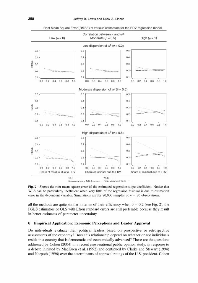
Figure 2 graphs the observed standard deviations of the estimates (RMSEs) as a function

of the percent of the total regression error that is due to sampling the dependent variable

for various values of h and q. The results are consistent with expectations. When h is low—when variance of the sampling errors in the dependent variable is fairly constant across

observations—all of the methods perform very similarly. Indeed, the lines representing

each of the methods in the top three panels of the graph are difficult to distinguish. As the

variation in the dependent variable sampling errors across observations (h) increases,

differences in the behavior of the estimators becomes apparent. In particular, when h is

large and little of the total regression residual stems from the mismeasurement in the

dependent variable (C is small), WLS produces estimates with approximately twice the

RMSEasOLS. Even as this fraction is increased,OLS continues to outperformWLS. Indeed,

until about 80% of the total error variance is the result of sampling error in the dependent

variable, OLS produces more efficient estimates than does the standard WLS approach.15

As anticipated, the FGLS estimators produce efficient estimates relative to OLS and

WLS, though in many cases the gains are quite modest. The ‘‘known variance’’ FGLS

estimator—the estimator that requires that the sampling variances of the dependent

variable observations be known—is generally more efficient than the proportional variance

estimator. This result follows from the fact that the proportional variance estimator

requires the estimation of one more parameter than does the known variance estimator.

Figure 3 graphs the observed standard errors across the 80,000 experiments as

a fraction of the average estimated standard errors of the various estimators against the

percent of the total regression error that is due to sampling error in the dependent variable.

Overall, these graphs are consistent with the expectations laid out earlier. OLS tends to

produce biased standard error estimates for high values of C, and WLS produces biased

standard error estimates except when C is very high (over 0.9). White’s standard error

estimates are generally effective, but in small samples, if robust standard errors are to be

employed, we recommend the more conservative Efron standard errors. With small n ¼ 30

in these simulations, the Efron estimates are more consistently accurate under each of the

nine scenarios considered. The two FGLS estimators produce quite accurate estimates of

parameter uncertainty; the known variance FGLS estimator works particularly well in all

cases. The proportional variance FGLS estimator is less successful when C is low, below

0.4, but generally performs no worse than WLS, especially with high values of h.Moving from the left-most to right-most panels of Fig. 3, one sees that as the correlation

between the independent variable and the sampling variances of the dependent variable

increases the bias of the OLS standard errors also increases.16 However, the Efron robust

standard errors are not similarly affected. It is interesting to note that even in the low

sampling error dispersion case (h ¼ 0.2), the observed OLS and WLS standard errors are

in some cases as much as 110% to 120% greater than the estimated standard errors. While

15When we ran the same simulation with a larger n ¼ 500, OLS was more efficient than WLS until about 90% ofthe total error variance was the result of sampling error in the dependent variable.

16This result is similar to those typically found in the heteroscedasticity literature (Greene 2003, p. 505).


all the methods are quite similar in terms of their efficiency when h ¼ 0.2 (see Fig. 2), the

FGLS estimators or OLS with Efron standard errors are still preferable because they result

in better estimates of parameter uncertainty.

6 Empirical Application: Economic Perceptions and Leader Approval

Do individuals evaluate their political leaders based on prospective or retrospective

assessments of the economy? Does this relationship depend on whether or not individuals

reside in a country that is democratic and economically advanced? These are the questions

addressed by Cohen (2004) in a recent cross-national public opinion study, in response to

a debate initiated by MacKuen et al. (1992) and continued by Clarke and Stewart (1994)

and Norpoth (1996) over the determinants of approval ratings of the U.S. president. Cohen

Fig. 2 Shows the root mean square error of the estimated regression slope coefficient. Notice that

WLS can be particularly inefficient when very little of the regression residual is due to estimation

error in the dependent variable. Simulations are for 80,000 samples of n ¼ 30 observations.


argues that ‘‘in the advanced industrialized nations of the West, leader approval will be

a function of prospective economic perceptions. In contrast, in the developing world and

among newer democracies, leader approval will be a function of retrospections’’ (2004,

p. 31). To conduct his analysis, Cohen uses survey data from the 2002 Pew Global

Attitudes Project, which was fielded between July and October 2002 in 44 countries

worldwide, including both developed and developing nations.17

Fig. 3 Shows the observed standard errors of the regression slope as a percentage of its average

estimated standard error. Notice that under some conditions OLS and WLS standard errors can be

very misleading. Simulations are for 80,000 samples of n ¼ 30 observations.

17The data set is free to download from the Pew Research Center for the People and the Press data archive athttp://people-press.org/dataarchive/. See the June 3, 2003, release of the report titled ‘‘Views of a ChangingWorld.’’ The Pew Global Attitudes Project bears no responsibility for the analyses or interpretations of the datapresented here.


http://people-press.org/dataarchive/

What makes this study particularly useful for our purposes is that at the time of his

analysis, Cohen had access only to the country-level toplines that were published in

Pew’s initial survey report. Therefore, the dependent variable was, by necessity, the

country-level proportion of respondents approving of their country’s president or prime

minister. This makes it impossible to draw inferences about the possible relationship

between individuals’ economic perceptions and their approval of their country’s chief

executive. Since that time, however, Pew has released the full data set of individual-level

survey responses. We employ these data to recast Cohen’s country-level analysis as

a multilevel model in which parameter estimates from within-country, individual-level

logit regressions are modeled as a function of economic development at the country level.

Cohen proposes a model that explains country-level presidential approval—‘‘the

percentage of respondents in each country who give the leader ‘a very good’ or ‘somewhat

good’ evaluation’’ (p. 33)18—as a function of three variables: economic ‘‘prospections,’’ eco-

nomic ‘‘retrospections,’’ and a dummy variable for whether or not a country is an ‘‘old’’

(economically advanced and stable) democracy.19 Cohen acknowledges the possibility of

nonconstant variance in his dependent variable as a result of the survey sample sizes

ranging from six countries with 500 respondents to India with 2189 respondents, so he

presents his linear regression results with both regular OLS standard errors and robust

Huber-White corrected standard errors.

Though Cohen does not present a weighted least squares (WLS) model in his results, one

could be easily estimated. Because the survey responses to the question of leader approval

arise from a random sample, we could estimate the standard error of that estimate as

bSEðPiÞ ¼ffiffiffiffiffiffiffiffiffiffiffiffiffiffiffiffiffiffiffiffiffiffiffiffiffiPið100� PiÞ

pni

;

where Pi is the percent support for the president or prime minister in a given country and niis the number of survey responses in country i. The inverse of these estimates would then

become the weights in a WLS regression. Looking more carefully at the standard errors of

the presidential approval ratings across the 41 surveyed countries in this example highlights

the concern associated with the application of a WLS model. Between the countries with

large and small sample sizes, the standard error estimates range only from a low of 0.77

(Uzbekistan) to a high of 2.23 (Canada). This disparity is not terribly large—nor is it ever

likely to be for cross-national public opinion studies in which the difference in the number

of interviews conducted in different countries will rarely exceed one order of magnitude. In

the notation of the Monte Carlo results presented earlier, this is a case in which the variation

in the sampling variances across observations, h, is small to moderate.

A good gauge of whether WLS is appropriate in this case is the R2 that the regression

would achieve if the only source of error was the uncertainty due to estimation of the de-

pendent variable. This R2 can be approximated as one minus the average sampling variance

of Y* (the residual variance) over the observed variance of Y* across countries (the total

variance).20 In this case, the average estimated sampling variance is about 2.8, while the

18The approval rating question—question 35b in the survey—was asked in 41 of the 44 study countries: all exceptChina, Egypt, and Vietnam.

19The economic retrospection and prospection questions are numbers 12 and 13, respectively. The model includestwo interaction terms to capture the possibility that the effect of economic evaluations differs between countriesthat are ‘‘old’’ and those that are not.

20The approximate R2 ¼ 1 � �x2i

Sy*where Sy* is the sample variance of the observed dependent variable across the

observations on the dependent variable.


cross-country variance of leader support is 513.7, so the R2 that one would expect is greater

than 0.99.21 Cohen reports an R2 from his OLS regression Model 3 (p. 35) to be a much

more modest 0.51. Thus, of the roughly 49% of the variance in leader approval that is not

accounted for by his model, only about 1% can be attributed to sampling errors in the mea-

surement of the true underlying leader approval. In the notation of the Monte Carlo exper-

iments,C, the fraction of the error due to estimation of the dependent variable, is quite small.

As such, WLS estimates are unlikely to be as reliable as the estimates from the OLS model.

With the individual-level data now available from Pew, we reanalyze Cohen’s claim

that ‘‘citizens in advanced democracies employ prospective evaluations, while citizens of

less advanced democracies employ retrospective assessments in evaluating the national

executive’’ (pp. 37–38) using a multilevel model that compares the OLS/robust standard

error, WLS, and FGLS approaches to EDV regressions.

We first run a series of 41 logistic regression models on the individual-level data within

the countries in the Pew study. The dependent variable in these models is whether or not

individuals have a ‘‘very good’’ or ‘‘somewhat good’’ opinion of their country’s president or

prime minister. The independent variables are the individual’s responses to the prospective

and retrospective economic evaluation questions; both are included in each multivariate

model as simultaneous controls. The prospective question is coded across five choices,

varying from whether the respondent expects economic conditions over the next 12 months

to ‘‘improve a lot’’ (1) all the way to ‘‘worsen a lot’’ (5). The retrospective question is coded

across four choices, varying from whether the respondent thinks the current economic

situation is ‘‘very good’’ (1) to ‘‘very bad’’ (4). Theory predicts negative coefficients on both

variables, indicating that as individuals take an increasingly worse view of their country’s

economy, they are less likely to support their country’s leader. This is indeed what we find:

all 41 of the ‘‘retrospective’’ coefficients are negative, as are 39 of the ‘‘prospective’’

coefficients; neither of the remaining two (in Brazil and Jordan) are statistically significant.

Cohen’s theory predicts cross-national heterogeneity in these logit coefficient estimates,

such that the effect of prospection should be greater, and the effect of retrospection lesser,

in countries that are advanced democracies versus those that are not. The coding scheme

Cohen devises for the dummy variable for ‘‘old’’ advanced democracies is primarily

a function of that country’s wealth; the seven countries coded as ‘‘old’’ are the seven

wealthiest in the sample.22 We therefore test Cohen’s prediction by regressing the within-

country coefficient estimates on prospection and retrospection on real per capita GDP in

2000.23 The results from these second-stage regressions are given in Table 3, for OLS with

Efron standard errors, WLS, and FGLS (known variance) models.

Contrary to Cohen’s hypothesis, there is no effect of wealth on the power of prospectiveeconomic considerations to predict leader approval. This finding may be confirmed

visually in the left-hand panel of Fig. 4. Individuals are more likely to hold an unfavorable

view of their leader as their opinion of the future economy worsens, regardless of the level

of wealth of the country in which they reside.

For our purposes, the retrospective models provide a more interesting example. Note

first that the sign on the coefficient of log of GDP per capita is opposite what Cohen

predicts. If citizens of poorer countries were more heavily economically retrospective

when forming opinions of their leader, then the coefficient on wealth would be positive,

21That is, 0.995 ¼ 1 � (2.8/513.7).22Cohen codes the ‘‘old democracy’’ variable 1 for Canada, France, Germany, Great Britain, Italy, Japan, and theUnited States, and 0 otherwise; see also Cohen’s footnote 5.

23These GDP data come from the World Bank 2002 World Development Indicators data set.


not negative. That is, the predicted coefficient on the within-country retrospective variable

would be more negative for poorer countries and increase to zero as countries increased in

wealth. This is not what we find (see the right-hand panel of Fig. 4). So, from a substantive

perspective, we conclude on the basis of this evidence that Cohen’s hypothesis is incorrect.

That said, while the coefficient on the log of GDP per capita is not significantly nonzero

in the OLS and FGLS models, the coefficient is significant in the WLS model. Why does

this difference arise, and which of these estimators is more likely to be producing accurate

estimates? Compared to Cohen’s country-level model discussed above, the average

estimated sampling error (0.023) is now much closer to the inter-country variance in the

retrospection coefficient estimate (0.055). Calculating as before, one would expect an R2

value of 0.58, but the R2 from the OLS regression in Table 3 is a mere 0.026. Of the 97%

of the variance in the retrospective logit coefficients not accounted for by the model, about

Table 3 Testing for cross-national parameter heterogeneity

Prospective models Retrospective models

OLSEfron SE WLS FGLS

OLSEfron SE WLS FGLS

Constant �0.261

(0.260)

�0.187

(0.254)

�0.221

(0.264)

�0.223

(0.274)

0.057

(0.261)

�0.141

(0.279)

log(per capita GDP) �0.041

(0.071)

�0.043

(0.068)

�0.046

(0.071)

�0.078

(0.074)

�0.146

(0.070)

�0.098

(0.075)

R2 0.008 0.026

r 0.221 0.189 0.234 0.176

Mean x 0.109 0.145

N 41 41 41 41 41 41

Note. The dependent variable is the logit coefficient from individual-level regression models in 41 countries. The

within-country logit models simultaneously regress leader approval against both prospective and retrospective

economic evaluations, thus generating the two sets of 41 coefficients used as the dependent variables here. Data

are from countries surveyed in the 2002 Pew Global Attitudes Project and from the World Bank 2002 WDI data

set. Standard errors are in parentheses.

3.0 3.5 4.0 4.5

−1.5

−1.0

−0.5

0.0

0.5

log of GDP per capita, 2000

3.0 3.5 4.0 4.5

log of GDP per capita, 2000

Firs

t−st

age

pros

pect

ion

logi

t coe

ffici

ent

−1.5

−1.0

−0.5

0.0

0.5

Firs

t−st

age

retr

ospe

ctio

n lo

git c

oeffi

cien

t

Fig. 4 Scatterplots of logit coefficients on economic prospection (left) and retrospection (right) from

41 country-level regressions of leader approval on those two variables, versus log of GDP per capita

in 2000. Vertical bars are 95% confidence intervals for each coefficient estimate. Best fit lines are

given for OLS (solid), WLS (dotted), and FGLS (dashed).


58% of that amount can be attributed to sampling errors in the estimation of the logit

coefficients. The remaining nearly 40% of the variance is being erroneously attributed to

measurement error by the WLS estimator. This is still a large enough amount that we

conclude that the WLS estimator has returned results that are misleading and would lead to

a researcher drawing false inferences.

7 Conclusion

Through a series of Monte Carlo experiments, we have demonstrated the following

relationships between estimation of EDV regression models using OLS, WLS, and a pair

of alternative FGLS estimators:

1. The larger the share of the regression residual that is due to sampling error in the

dependent variable, the less efficient OLS is and the more efficient WLS is.

2. WLS leads to greater overconfidence (downwardly biased standard errors) the

smaller the fraction of the error variance attributable to sampling error in the

dependent variable.

3. OLS standard errors are increasingly biased as the correlation between the

independent variables and the variance of the sampling error in the dependent

variable increases and as the fraction of the total regression error variance due to

sampling error in the dependent variable increases.

4. White’s (1980) and Efron (for small samples) heteroscedastic consistent standard

error estimators are generally reliable (no over- or under-confidence), though OLS

may be quite inefficient.

5. The FLGS estimators presented above produce efficient estimates (relative to OLS)

if a sufficiently high fraction of the total regression error variance is due to sampling

error. The standard errors of these estimators generally produce less overconfidence

than is found using OLS and WLS.

The results presented in this article suggest that information about the variance of the

sampling errors in estimated dependent variables should be used with caution. The usual

approach of weighting the dependent variable by the inverse of the standard errors of the

dependent variable estimates will in most cases lead to inefficient parameter estimates and

overconfidence in these estimates. This overconfidence can be very large. In some cases,

the true uncertainty in the parameter estimates was nearly double the WLS estimated

parameter uncertainty. Discarding information about the sampling errors in the

observations on the dependent variable and fitting OLS with White’s or Efron robust

standard errors is generally superior to the WLS approach. Indeed, OLS with robust

standard errors is probably the best approach, except when information about the sampling

errors in the dependent variable is not only available, but highly reliable.

However, when reliable information about the sampling variances of the estimated

dependent variable is available, the two FGLS approaches presented above will yield

generally superior results to OLS. In some of the cases considered, the gain in efficiency

was substantial. These FGLS estimators are easy to implement and allow the analyst not

only to achieve efficient parameter estimates, but also to estimate the fraction of the total

regression error that is due to sampling errors in the measurement of the dependent variable.

References

Anderson, Christopher J., and Yuliya V. Tverdova. 2003. ‘‘Corruption, Political Allegiances, and Attitudes

toward Government in Contemporary Democracies.’’ American Journal of Political Science 47:91–109.


Banducci, Susan A., Jeffrey A. Karp, and Peter H. Loedel. 2003. ‘‘The Euro, Economic Interests and Multi-

level Governance: Examining Support for the Common Currency.’’ European Journal of Political Research

42:685–703.

Bryk, Anthony, and Stephen W. Raudenbush. 1992. Hierarchical Linear Models: Applications and Data

Analysis Methods. Newbury Park, CA: Sage.

Burden, Barry, and David Kimball. 1998. ‘‘A New Approach to the Study of Ticket Splitting.’’ American

Political Science Review 92:533–544.

Clarke, Harold D., and Marianne C. Stewart. 1994. ‘‘Prospections, Retrospections, and Rationality: The ‘Bankers’

Model of Presidential Approval Reconsidered.’’ American Journal of Political Science 38:1104–1123.

Cohen, Jeffrey E. 2004. ‘‘Economic Perceptions and Executive Approval in Comparative Perspective.’’ Political

Behavior 26:27–43.

DeGroot, Morris H., and Mark J. Schervish. 2002. Probability and Statistics, 3rd ed. New York: Addison

Wesley.

Efron, Bradley. 1982. The Jackknife, the Bootstrap and Other Resampling Plans. Philadelphia, PA: Society for

Industrial and Applied Mathematics.

Greene, William H. 2003. Econometric Analysis, 5th ed. Englewood, NJ: Prentice Hall.

Guerin, Daniel, Jean Crete, and Jean Mercier. 2001. ‘‘A Multilevel Analysis of the Determinants of Recycling

Behavior in the European Countries.’’ Social Science Research 30:195–218.

Hanushek, Eric A. 1974. ‘‘Efficient Estimators for Regressing Regression Coefficients.’’ American Statistician

28:66–67.

Hanushek, Eric A., and John E. Jackson. 1977. Statistical Methods for Social Scientists. New York: Academic.

Herron, Michael C., and Kenneth W. Shotts. 2003. ‘‘Using Ecological Inference Point Estimates as Dependent

Variables in Second-Stage Linear Regressions.’’ Political Analysis 11:44–64.

Jusko, Karen Long, and W. Phillips Shively. 2005. ‘‘Applying a Two-Step Strategy to the Analysis of Cross-

National Public Opinion Data.’’ Political Analysis. doi:10.1093/pan/mpi030.

Kaltenthaler, Karl C., and Christopher J. Anderson. 2001. ‘‘Europeans and Their Money: Explaining Public

Support for the Common European Currency.’’ European Journal of Political Research 40:139–170.

King, Gary. 1997. A Solution to the Ecological Inference Problem: Reconstructing Individual Behavior from

Aggregate Data. Princeton, NJ: Princeton University Press.

Long, J. Scott, and Laurie H. Ervin. 2000. ‘‘Using Heteroscedasticity Consistent Standard Errors in the Linear

Regression Model.’’ American Statistician 54:217–224.

Lubbers, Marcel, Merove Gijsberts, and Peer Scheepers. 2002. ‘‘Extreme Right-Wing Voting in Western

Europe.’’ European Journal of Political Research 41:345–378.

MacKinnon, James G., and Halbert White. 1985. ‘‘Some Heteroscedasticity Consistent Covariance Matrix

Estimators with Improved Finite Sample Properties.’’ Journal of Econometrics 29:305–325.

MacKuen, Michael B., Robert S. Erikson, and James A. Stimson. 1989. ‘‘Macropartisanship.’’ American Political

Science Review 83:1125–1142.

MacKuen, Michael B., Robert S. Erikson, and James A. Stimson. 1992. ‘‘Peasants or Bankers? The American

Electorate and the U.S. Economy.’’ American Political Science Review 86:597–611.

Maddala, G. S. 2001. Introduction to Econometrics, 3rd ed. West Sussex: John Wiley and Sons.

Norpoth, Helmut. 1996. ‘‘Presidents and the Prospective Voter.’’ Journal of Politics 58:776–792.

Oppenheimer, Bruce. 1996. ‘‘The Importance of Elections in a Strong Congressional Party Era.’’ In Do Elections

Matter? eds. Benjamin Ginsberg and Alan Stone. Armonk, NY: M. E. Sharpe, pp. 120–139.

Patel, Jagdish K., and Campbell B. Read. 1996. Handbook of the Normal Distribution. New York: Marcel

Dekker.

Peffley, Mark, and Robert Rohrschneider. 2003. ‘‘Democratization and Political Tolerance in Seventeen

Countries: A Multi-level Model of Democratic Learning.’’ Political Research Quarterly 56:243–257.

Rohrschneider, Robert, and Stephen Whitefield. 2004. ‘‘Support for Foreign Ownership and Integration in Eastern

Europe; Economic Interests, Ideological Commitments, and Democratic Context.’’ Comparative Political

Studies 37:313–339.

Saxonhouse, Gary R. 1976. ‘‘Estimated Parameters as Dependent Variables.’’ American Economic Review

66:178–183.

Steenbergen, Marco R., and Bradford S. Jones. 2002. ‘‘Modeling Multilevel Data Structures.’’ American Journal

of Political Science 46:218–237.

Taylor, D. Garth. 1980. ‘‘Procedures for Evaluating Trends in Public Opinion.’’ Public Opinion Quarterly

44:86–100.

White, Halbert. 1980. ‘‘A Heteroscadastically-Consistent Covariance Matrix Estimator and a Direct Test for the

Heteroscasticity.’’ Econometrica 48:817–838.


estimating regression models in which the dependent ... · estimating regression models in which...

Documents