estimating the economic impacts of climate change using

NBER WORKING PAPER SERIES

ESTIMATING THE ECONOMIC IMPACTS OF CLIMATE CHANGE USING WEATHER OBSERVATIONS

Charles D. KolstadFrances C. Moore

Working Paper 25537http://www.nber.org/papers/w25537

NATIONAL BUREAU OF ECONOMIC RESEARCH1050 Massachusetts Avenue

Cambridge, MA 02138February 2019

An earlier version of this paper was presented at a workshop on “Advances in Estimating the Economic Effects of Climate Change Using Weather Observations” at Stanford University (Institute for Economic Policy Research (SIEPR), held in May 2017; the authors are grateful to workshop participants for comments and insights. The views expressed herein are those of the authors and do not necessarily reflect the views of the National Bureau of Economic Research.

NBER working papers are circulated for discussion and comment purposes. They have not been peer-reviewed or been subject to the review by the NBER Board of Directors that accompanies official NBER publications.

© 2019 by Charles D. Kolstad and Frances C. Moore. All rights reserved. Short sections of text, not to exceed two paragraphs, may be quoted without explicit permission provided that full credit, including © notice, is given to the source.

Estimating the Economic Impacts of Climate Change Using Weather ObservationsCharles D. Kolstad and Frances C. MooreNBER Working Paper No. 25537February 2019JEL No. H41,Q51,Q54

ABSTRACT

This paper reviews methods that have been used to statistically measure the effect of climate on economic value, using historic data on weather, climate, economic activity and other variables. This has been an active area of research for several decades, with many recent developments and discussion of the best way of measuring climate damages. The paper begins with a conceptual framework covering issues relevant to estimating the costs of climate change impacts. It then considers several approaches to econometrically estimate impacts that have been proposed in the literature: cross-sections, linear and non-linear panel methods, long-differences, and partitioning variation. For each method we describe the kind of impacts (short-run vs long-run) estimated, the type of weather or climate variation used, and the pros and cons of the approach.

Charles D. KolstadStanford University366 Galvez Street (Room 226)Stanford, CA 94305-6015and [email protected]

Frances C. MooreDepartment of Environmental Science and Policy 1023 Wickson Hall University of CaliforniaDavis One Shields AvenueDavis, CA [email protected]

Draft: 30 January 2019 1

Estimating the Economic Impacts of Climate Change Using Weather Observations* Charles D. Kolstad1 and Frances C. Moore2

Abstract

This paper reviews methods that have been used to statistically measure the effect of climate on economic value, using historic data on weather, climate, economic activity and other variables. This has been an active area of research for several decades, with many recent developments and discussion of the best way of measuring climate damages. The paper begins with a conceptual framework covering issues relevant to estimating the costs of climate change impacts. It then considers several approaches to econometrically estimate impacts that have been proposed in the literature: cross-sections, linear and non-linear panel methods, long-differences, and partitioning variation. For each method we describe the kind of impacts (short-run vs long-run) estimated, the type of weather or climate variation used, and the pros and cons of the approach.

I. INTRODUCTION

Physical changes in the climate due to greenhouse gas emissions are now well-documented, and future changes due to unmitigated greenhouse gas emissions are generally well understood. But quantifying the economic consequences of changes in temperature, rainfall, sea-level, or other climate variables has long been recognized as extremely challenging. Doing so is critical, however, to developing informed mitigation and adaptation policy: optimal mitigation rates depend on the severity of global impacts, while adaptation policies in particular places and sectors must be designed to address the expected damages in those areas.

Although early studies estimating the economic damages associated with climate change used process models to simulate the effects of changing climate variables (e.g., Smith and Tirpak, 1989), much recent work has instead focused on statistical approaches using historical data. The benefit of these models is that they are based on observed relationships in real-world settings. For the most part, these models do not assume any theory-based structural relationships among variables (ie, they are reduced-form specifications). Initial approaches used one time point, exploiting cross-sectional variation in climate to estimate the marginal effect of long-run changes in the distribution of temperature and rainfall (for instance Mendelsohn, Nordhaus, & Shaw, 1994). Since the turn of the century, though, there has been an explosion of literature using data which varies over both space and time (panel data) to estimate the effects of inter-annual variation in weather on economic outcomes (for reviews, see Carleton & Hsiang, 2016 and Dell, Jones, & Olken, 2014).

1 Stanford Institute for Economic Policy Research (SIEPR), Precourt Institute for Energy and Department of Economics, Stanford University; NBER; and UC Santa Barbara. 2 Department of Environmental Science and Policy, University of California Davis. *An earlier version of this paper was presented at a workshop on “Advances in Estimating the Economic Effects of Climate Change Using Weather Observations” at Stanford University (Institute for Economic Policy Research (SIEPR), held in May 2017; the authors are grateful to workshop participants for comments and insights.


Panel approaches have significant advantages over cross-sectional regressions, not only because of the expanded set of data used (varying in time and space) but also because fixed-effects are able to control for many unobserved omitted variables, particularly time-invariant variation across space, which is often a concern in this setting (Deschênes & Greenstone, 2007). However, the benefit of using fixed-effects is offset by the fact that climate is basically fixed over time in most econometric applications, making identification of the direct effect of climate on impacts difficult.

Furthermore, there have long been concerns that the effect of inter-annual weather variation on impacts cannot be used to identify the effect of climate changes because the response to short-run weather fluctuations may be fundamentally different than the response to a permanent change in the distribution of those fluctuations (ie, the climate). This difference is due to adaptation: people and firms may respond differently (adapt) to permanent changes in the expected distribution of weather than to short-term and unanticipated fluctuations in weather. If this adaptation is significant then the impact of weather fluctuations may not be a good analog for the effect of a permanent change in the climate.

The question of how best to estimate the effects of long-run changes in climate has long been one of contention. In their review of studies using panel data to estimate the effect of weather fluctuations on economic outcomes, Dell et al. (2014) identify three high priority areas for future research, concluding with: “Third, and perhaps most importantly, bridging from the well-identified results from short-run shocks [weather] to longer-run outcomes [climate] is an important dimension for future work.” (p. 790). Resolving this issue is essential if recent empirical results are to be used to inform damage functions and ultimately the social cost of carbon used in the cost-benefit analysis of climate policy (Burke et al., 2016; Diaz & Moore, 2017; Greenstone et al, 2013).

Because of the importance of this topic, significant research attention has been devoted recently to the question of how to statistically identify climate change impacts using historical panel data. A number of new approaches have been proposed that exploit the richness of many panel data-sets, which often contain information on inter-annual weather variation, long-term differences in climate, and medium-term (decadal) changes in average weather conditions. Comparing the responses to these different types of variation can give information on the importance of private adaptation and a more accurate estimate of climate change impacts.

This paper begins by establishing a conceptual framework for thinking about climate, weather, adaptation, and the overall economic costs of climate change. The paper then reviews different approaches that have been proposed for econometrically estimating the effects of climate change, both the classic cross-sectional approach, more recent panel approaches using interannual weather variation, and very recent hybrid approaches that use a mix of cross-sectional and interannual variation in order to better identify climate change impacts.

II. CONCEPTUAL FRAMEWORK

A. Climate and Weather

A rigorous discussion of methods to identify climate change impacts must begin with a definition of climate, climate change, and weather. Strictly speaking, weather is the instantaneous condition of the


atmosphere at a particular location (see Oxford English Dictionary). The weather at any given point can be described not just by temperature and rainfall, but by numerous other variables such as air pressure, wind speed and direction, relative humidity, cloud cover, and wind shear, to name just a few. Weather is a complex multi-variate and time-varying concept.

For most economic and policy applications, representing actual weather is impractical and summary statistics are generally sufficient. These summary variables reduce the dimensionality of weather while retaining relevant information for the application. The choice of summary statistic will depend on the application – in agriculture, annual or monthly growing and killing degree-days3 and total monthly or annual precipitation have been useful. For human health, peak wet-bulb temperature may be more relevant while heating and cooling degree days are often used to model energy demand. In this paper we will refer to the time- and space-varying summary or sufficient statistic as the “weather statistic” or simply the “weather,” keeping in mind that the exact nature of that summary statistic will depend on the application, and that this is sometimes a multi-variate quantity.

Climate, on the other hand, is classically defined as the probability distribution over weather outcomes. In the economic and policy context (this paper), climate will be defined to be the full, possibly joint, probability distribution of the relevant weather statistic(s). Climate change, therefore is defined as a change in the probability distribution from which the weather statistic is drawn each time period. The goal of empirical studies estimating climate impacts is to use historical data to infer the welfare consequences of future changes in the climate (weather distribution).4 For further discussion of these issues see Hsiang (2016) and Lemoine (2018).

B. Welfare Consequences of Changes in Weather and Climate

Ultimately we are interested in the welfare consequences of climate change. Conceptually, we start with a simple representation of a production process (eg, Pope and Chavez, 1994; Kelly et al, 2005; Hsiang, 2016), whereby output is influenced by two sets of variables: weather realizations and production choices. Weather is not controllable by the economic agent and is generally unanticipated; production choices (eg, what to plant and when, or how much capital to invest) are decisions made by the economic agent and are based on a host of factors, including prices and expectations about stochastic weather.

3Degree days are daily temperature differences summed over a period of time. Usually the temperature differences are the difference between the average temperature on a day and some base temperature. For instance, heating degree days are defined by the US EIA as the extent to which temperature is less than a base of 65oF. The agricultural literature often defines growing degree days as the extent to which daily temperature exceeds 8oC for the days in a growing season and similarly, killing degree days are defined with respect to a base temperature of 29oC (eg, Butlet and Huybers, 2012). 4 The World Meteorological Organization (WMO) requires member nations to compute 30-year “climate normals” - the annual or monthly mean and variance of weather variables over a defined 30 year period and to update these every 30 years (Arguez & Vose, 2011). In statistical terms, this simply means that the climate (weather distribution) is estimated using a 30 year sample, although only measuring two moments (mean and variance) may not be the best way to estimate the underlying distribution of a weather statistic.


Even in a stationary climate, agents face variation in the weather arising from chaotic fluctuations in the earth system, termed “internal” or “natural” variability in the climate science literature (Deser, Knutti, Solomon, & Phillips, 2012). Assuming agents know the stationary climate distribution they face, they will make investments to reduce the net losses associated with this variability, balancing the costs of such investments with the bentifts of lower impacts of weather fluctuations. A good example of this is investments in irrigation capital to reduce the losses from variable natural precipitation – these investments may be profitable in a dry or highly variable climate, but may not be justified in a wetter climate.

Similarly, when climate changes (and the agent knows it) and thus the realizations of weather change, the agent can take change its production choices, adapting to the change in climate as best it can. Determining optimal responses to a changed climate involves trading off the costs of such actions with the benefits, in terms of net expected losses from the new distribution of weather. Such actions are termed private adaptation in the context of climate change; in economics, this is simply the natural adjustment of an economic agent to changed technologies or prices.5 The net cost of the change in climate is the sum of the net change in production expenditures less the net value gain in expected output. For instance if climate change consists of a drop in annual mean precipitation, then adaptive action may be costly investments in irrigation and water storage; output losses will be changes in expected output, taking into account the change in adaptive responses. The net impact, the costs of adaptive action plus the loss in expected output after adaptive action has occurred, will be the damage from the change in climate. On net, the costs of the climate change may be positive or negative. (It is also easy to see that the impacts of changes in weather, represented in most panel models, does not capture the full impacts of climate change since adaptive actions are ignored.)

Both expectations and fixed capital investments can adjust in response to permanent changes in climate but not in response to short-term variation in weather. We can therefore define the short-run response to a change in climate as the effect of a shift in the true climate keeping expectations, beliefs and, by extension, investments fixed (Kelly et al, 2005). This short-run response could be estimated by observing the effects of weather fluctuations. The long-run response in contrast is the effect of a change in climate after both beliefs and capital investments have been allowed to equilibrate to the new climate. As long as there are management or investment adaptations that agents can take to improve outcomes under the changed climate, the short- and long-run effects of climate change will be different.

To complicate the issue a bit more, the change in climate may be instantaneous or gradual and the impacts will be different in those two cases. Consider a change in the climate distribution. Firstly, we consider an instantaneous shift in the climate (Figure 1a). Though not a realistic representation of climate change, this will provide some intuition for discussion of a more gradual process. Since the climate distribution can only be inferred from experience of weather, this sudden shift is not initially observed. Instead, the first draws from the changed climate may be interpreted only as unusual weather events. Gradually though, evidence in the form of repeated weather observations will lead an agent to update their beliefs regarding the underlying climate distribution. Conditioned on this new belief, the

5 Some adaptation is not taken by individual agents but rather collectively. Examples include investments in flood control or public infrastructure. Typically governments are involved in such public adaptation and market failures resulting from collective action problems may result in under-provision of these adaptations. These inefficiencies are not considered further in this paper, which focuses on private adaptation.


agent will re-optimize their investments and management to maximize welfare under the new climate distribution.

Figure 1b shows expected welfare under this simple representation of climate change. Climate change lowers welfare both because of inherently worse outcomes under the changed climate and because agents are initially not adapted to or even informed about the new climate. The equilibrium costs of a shift in climate are defined as the residual loss in welfare , including adaptation costs, after adjusting to the new climate (lightly shaded area, Figure 1b). Adjusment costs are additional costs associated with being imperfectly adjusted to a particular climate (darker shaded area, Figure 1b). Adustment costs can arise both from incorrect beliefs about the state of the climate distribution (“mistakes”), and from the time it takes to replace obsolete factors of production (eg, captial). Both beliefs and factor investments will adjust over the long-run, but not in response to short-run fluctuations in weather (for non-climate adjustment cost applications see Abel and Eberly, 1994; Cooper and Haltiwanger, 1995). The magnitude of adjustment costs will depend on the net benefits of adaptation options and the time-scale over which adaptation occurs (Kelly, Kolstad and Mitchell, 2005). Certain sectors in which long-lived capital stocks are important, such as forestry or coastal defenses, are likely to have larger adjustment costs than others.

A more realistic representation of climate change accounts for the fact that it is not a step change, but instead accumulates gradually over time. The concepts of equilibrium and adjustment costs translate to this setting. Figure 1c shows the same change in climate as in Figure 1a, but occuring gradually over 25 years. Figure 1d shows changes in welfare given the same response function and adjustment rate shown in Figure 1b, but occuring in response to the gradually changing climate. Imperfect adjustment to the climate at any given point in time still results in a wedge between the equilibrium welfare and that achieved by agents with imperfect information (i.e. adjustment costs). Welfare only converges to the equilibrium value over time, once the climate has stabilized. If climate change is slower relative to the rate of adjustment, or if agents are able to anticipate future climate change then adjustment costs will be smaller.

C. Quantifying Climate Change Damages

Full accounting of the net economic costs of climate change will include both equilibrium costs (including the residual damages after full adaptation and the costs of adaptation) and adjustment costs (which are temporary and will depend on the rate of adaptation and the effectiveness of adaptation options). Few empirical methods are able to fully estimate all these aspects of climate damages. There are some special cases, however, where adjustment costs are small or adaptation opportunities are minimal so that quantifying the economic damages associated with climate change is somewhat easier. It remains the case that only looking at how economic output changes with weather shocks cannot be used as a proxy for the economic impacts of a change in climate, except in certain cases.

One special case is where the potential margins for adaptation and adjustment are ineffective or very limited. In this case the short-run responses to weather changes and the long-run responses to climate change will be nearly identical, so that knowing either is sufficient to characterize climate change damages. Hsiang (2016) has used the envelope theorem to suggest that, in cases where adaptation technologies are continuous, adaptation is unlikely to be significant, at least for marginal changes in the


climate. The corollary though is provided by Guo and Costello (2013), who show that, in cases where adaptation technologies are discontinuous, the potential benefits of adaptation are theoretically unbounded, even for marginal changes in climate.

A second special case is one in which adaptations may be beneficial but the rate of adaptation is fast. In this case equilibrium costs will make up the vast majority of climate change damages and adjustment costs can be safely ignored as of second order importance. In this setting, only the residual damages under equilibrium and the adaptation costs need be known in order to quantify climate damages. Some authors have argued that because climate changes only over decades to centuries, economic adjustment rates will be relatively rapid and adjustment costs correspondingly small (Schlenker, Hanemann, & Fischer, 2005). Unless either of these conditions applies, however, fully understanding the costs of climate change requires characterizing both equilibrium and adjustment costs and therefore requires knowing both the short- and long-run response to a change in climate.

In the following section we review the reduced form empirical methods that have been used to estimate the effects of weather and climate, with a view to informing estimates of climate change damages. A long-standing question in the literature has surrounded the trade-off between improving confidence in empirical estimates using fixed-effects to control for unobserved omitted variables and estimating the long-run, equilibrium response to climate change. We first review this debate through a discussion of cross-sectional and linear panel models, and then review a more recent set of methods, which we collectively term “hybrid approaches”, that combine the cross-sectional and time-series variation in panel data to produce response functions more relevant to climate change impacts while retaining the benefits of fixed effect specifications.

III. EMPIRICAL APPROACHES

Given the conceptual framework outlined above, it is clear that, depending on the setting, the short-run response, long-run response, and rate of adaptation could all be relevant to fully quantifying climate change impacts. Various empirical approaches have been proposed that can estimate some or all of these. Here we review some of the most common econometric approaches, as well as emerging techniques that combine the short- and long-run variation in panel data in order to improve quantification of climate change impacts (see also Hsiang, 2016; Blanc and Schlenker, 2017; Dell, Jones, and Olken, 2014). For each technique, we will cover the kind of climate or weather variation used, a stylized estimating equation, the ability of the method to estimate equilibrium and / or adjustment costs, and any threats to unbiased identification. Some authors have pointed out the trade-off between using variation over long timescales (which is most relevant for identifying climate change impacts if adaptation is significant), and the improved identification enabled by higher frequency variation (Schlenker, 2010; Hsiang and Burke, 2014). In this section we will describe these tradeoffs systematically for the various approaches proposed in the literature for identifying climate impacts. Table I summarizes some of the differences among these various approaches, along with a stylized estimating equation for each method.

A. Cross-Section

The first econometric approach to estimating climate change impacts used cross-sectional variation in long-term climates to estimate the equilibrium (i.e. long-run) effects of a change in climate. Pioneered


by Mendelsohn, Nordhaus and Shaw (1994),6 this approach compares outcomes across space, essentially using hotter places with the current climate as analogs for currently colder places under a changed climate. Since the differences in climate observed across space are long-term and assumed stable, it is reasonable to assume that agents will have fully adjusted investments and management practices to maximize output under the climate they face. The cross-sectional approach therefore gives an estimate of the long-run response to climate change and can be used to estimate the equilibrium costs of a change in climate.

The econometric specification involves an economic outcome of interest on the left hand side of the equation, varying over space at an instant of time, with a function of climate, various other observable controls, and an error term on the right hand side of the equation (see Table 1, row 1). Note that panel data, where available, can be used to estimate pooled cross-sectional models (Masetti and Mendelsohn, 2011; Schlenker, Hanemann and Fischer, 2006). However, since in most settings relevant to climate change, cross-sectional variation is large relative to time-series variation, models that do not use spatial fixed-effects will have the same benefits and concerns regarding identification as standard cross-sections.

There are a number of potential problems with this approach. One important question that has received much attention is whether the set of observable cross-sectional variables included as controls are able to remove all confounding variables that might otherwise bias estimates of the effect of climate on the left-hand side economic outcome. If unobservable factors are correlated with the climate and also affect the outcome, then the estimated effect of climate will be biased. For instance, in an agricultural setting, soil quality often varies with climate, but also affects productivity and therefore land values. To the extent soil quality is observed, it can be controlled for in the regression, but there is always a concern that unobservable characteristics may be important. Schlenker, Hanemann, and Fisher (2005) show that the estimated effect of climate on land values differs significantly between irrigated and non-irrigated counties, suggesting that ignoring historic investments in irrigation infrastructure would lead to bias. Ortiz-Bobea (2016) proposes an approach to account for time-invariant unobservables by controlling for observable characteristics of neighboring counties and finds this significantly changes the estimated effect of climate change on US agriculture.

A second challenge in this class of regressions is how to define the climate variables used as explanatory variables since, as discussed above, the climate itself is not observable. If the climate is stationary (or the relevant agents believe the climate is stationary) then the historic distribution of the relevant summary weather statistic can be used as a noisy estimate of the climate. It is common in the literature to assume a stationary climate, using the past 30-years of weather observations to estimate the climate (Mendelsohn et al., 1994; Mendelsohn & Reinsborough, 2007). However, if agents recognize the climate is non-stationary then the question of how to estimate the effect of climate is more complicated, with the largest effect on forward-looking outcomes such as land prices. Severen, Costello and Deschenes

6 A much earlier paper (Johnson and Haigh, 1970) take a very similar approach, motivated by weather modification policy. They estimate a cross-sectional model of land prices in 1964, as influenced by soil characteristics and climatic variables, among other exogenous parameters. As noted by Aufhammer et al (2013), as early as 1925, researchers were examining the effect of weather on economic output. However, the Mendelsohn et al (1994) analysis is more widely known and much more specifically oriented towards the issue of economic impacts of a change in climate.


(2016) for instance show evidence that climate change projections are already capitalized into agricultural land markets, meaning using only past observations of weather to estimate climate will result in a biased estimate of climate change impacts. The ideal variable to use would be agent’s beliefs about the weather distribution, but this is not usually directly observable.

The main benefit of the cross-sectional approach is that it yields the long-run, equilibrium effects of climate change, incorporating the net benefits of all possible margins of adaptation. If adjustment costs are small, either because they occur rapidly relative to the rate of climate change or because the margins of adjustment are limited, then an unbiased cross-sectional regression is sufficient to estimate the impacts of climate change. However, some have argued that long-lived institutions and path-dependence of institutional and economic processes mean adjustment costs may be substantial, or even constitute the vast majority of climate change damages. The implication is that in such a case, the cross-section, by only estimating equilibrium costs, would substantially under-estimate total impacts. (Quiggin & Horowitz, 1999).

B. Linear Panel

In response to identification concerns in cross-sectional approaches, the past decade has seen a growth in the use of panel data to estimate weather impacts, though the effects of climate are harder to identify (Carleton & Hsiang, 2016; Dell et al., 2014). Because panel data includes observations of many units in many time periods, fixed-effects can be used to control for all time-invariant differences between units and all common differences between time periods. A stylized estimating equation can be written with the economic outcome of interest on the left hand side of the equation, varying over time and space. The right hand side of the estimating equation is linear in weather (varying over time and space), a fixed effect varying over space, a fixed effect varying over time plus an error term (Table 1, row 2). The flexible control for unobservable differences provided by the fixed effects increases confidence that omitted variables are not biasing the estimated relationship, relative to a cross-sectional approach. (Note that non-linear panels have substantively different qualities in terms of representing adaptation and therefore are dealt with in the next section.)

Estimation of the coefficient on weather in this panel setting comes from averaging the effect of time-series variation in weather in each location. Permanent differences in climate (used in the cross-section approach) are captured by the location fixed-effect, making identifying the effect of climate, as distinct from other location invariates, difficult. Statistical power in explaining weather comes from using the deviation of the weather statistic in a particular year from its average value in each location. Common trends in weather (e.g. due to climate change) are removed with the time fixed-effect. Moreover, since non-stationarity could result in spurious correlations, gradual changes in weather over time are also often removed with smooth, region-specific time trends. This means the variation used for estimation in this setting tends to come from temporary, and unexpected weather shocks (Schlenker, 2010).

The use of weather variation that is unexpected and temporary for estimation means that this method gives an estimate of the short-run response to climate change: we would not expect capital investments, factor use, or beliefs about the average climate to adjust in response to short-term weather shocks. If opportunities for adaptation and adjustment are small then the short-run and long-run response will be similar and either can be used to estimate the impacts of climate change. Hsiang (2016) uses the envelope theorem to argue that this is the case in situations where adaptation technologies are continuous. In cases where the adaptation potential is substantial, however, using the short-run


response to infer climate change impacts will result in a biased estimate of damages because it does not account for longer-term changes people can make to improve outcomes under a permanent change in climate.

Although time-invariant omitted variables are not a concern in the linear panel setting (they are absorbed in the location fixed effect), there are some cases in which time varying omitted variables could raise issues when using the estimate to calculate climate change impacts (beyond the questions of adaptation described previously). An example is the effect of temperature on mortality. Temperature and relative humidity are correlated and both affect mortality rates, but they are projected to change in opposite ways with climate change (Fischer & Knutti, 2013). Therefore a panel regression of mortality rates on temperature alone, without controlling for relative humidity, could give a biased estimate of climate change effects on mortality.

C. Emerging Hybrid Approaches

The cross-section and panel approaches described above are well established in the literature and have given rise to a well-worn dichotomy between the benefits of clean identification of the impacts of weather and short-run impacts using a panel estimate and the benefits of accounting for long-run adaptations and identifying the role of climate using the cross-section. However, a number of emerging approaches are using panel data in innovative ways, combining cross-sectional, inter-annual, and decadal variation in weather to estimate climate change effects while still controlling for unobservable confounding variables. Here we characterize these approaches, grouping them into three groups: heterogeneous marginal effects, partitioning variation, and long-differences.

1 Heterogeneous Marginal Effects

It is unlikely warming will have the same effect in cold places as in hot places, meaning a linear response function with a constant marginal effect may often be inappropriate for modeling the effect of climate change. In other words, in this example, it is likely that the marginal effect of warming will vary as a function of climate, implying the need for a non-linear response function. Because panel data contains information on the effect of inter-annual weather variability in multiple locations, it can be used to model this heterogeneity. Two approaches have been proposed to estimate heterogenous marginal effects: non-linear panel models and multi-stage models.

Non-linear panel models are similar to linear panel models except they involve a nonlinear function of weather. The fact that weather enters non-linearly means that the marginal effect of a change in weather is itself a function of weather. (For instance, if the function is a quadratic, then the marginal effect of weather is linear.) Although the effect of climate on the level of economic value is removed through the location fixed-effect, the expected marginal effect of a change in weather in a particular location depends on the distribution of the weather; i.e. on the climate in that place. Therefore, the non-linearity in weather implicitly allows the marginal effect of weather to vary with climate across locations.

Using the example of temperature, because the marginal effect of weather is allowed to vary cross-sectionally with climate in a non-linear panel, time-series variation in weather in places with hot and cold climates is used to estimate the gradient of the hot and cold support respectively. If long-run


adaptation alters the marginal response to weather variation, then these effects will be captured in the panel estimates, despite the fact that the location fixed-effect captures all time invariant differences between locations. In other words, unlike the linear specification discussed in section 2, non-linear panel estimates cannot be interpreted as only the short-run response to climate change (though they still are not able to fully account for the effect of a change in climate on output).

Figure 2 shows schematically how non-linear specifications, by allowing for varying marginal effects of warming, imply that the estimated effects are a mix of long- and short-run responses, if adaptation is possible. In this hypothetical panel dataset there are observations of weather and economic value from only two locations (eg, hot and cold), with the distribution of weather (climates) shown by the red (warmer) and blue (cooler) distributions. In the top panel (A), the climates are quite different; in the lower panel (B) the climates “overlap”. There are also two technologies available to agents – one that performs best in hot climates and one that performs best in cold climates: the true relationship between weather and economic value (y) in the two locations is shown as solid lines, and assumed to be piecewise linear for simplicity. Following Schlenker and Roberts (2009), note that both places are adapted to the level of heat exposure they face so that the warmer location (red) does best for its climate and the cooler location (blue) is more productive when temperatures are lower.

In panel A, the climates are quite distinct so that only observations from the cool location are used to estimate the slope of the cooler part of the value function and only observations from the warm location are used to estimate the hotter part. The resulting response function (black dashed line) captures the low heat sensitivity of a location that has adapted over the long-run to a hotter climate, not the high heat sensitivity of a cool location temporarily exposed to hot temperatures. It cannot be interpreted as the short-run response to climate change because it does not capture the large sensitivity to heat stress of the cooler location. Nor can it be interpreted as the long-run response because it does not capture the lower productivity associated with switching to more heat-tolerant technologies.7

In panel B, the climates of the two locations overlap so that the estimated response function is a weighted average of the locally adapted and un-adapted effects. In general, since most observations of hot weather come from places with hot climates (and conversely for cool weather), the estimated responses will be heavily influenced by locations adapted to that type of weather, though the exact weighting will depend on the pattern of time-series and cross-sectional variation in the data and the functional form of the response curve.

Deryugina and Hsiang (2017) provide a theoretical development of this, as well as an empirical application estimating the effect of climate on income in the United States. They suggest that the marginal effect of weather on output is the same as the marginal effect of climate on output, a relatively new result which has not yet been widely embraced or confirmed in the literature. It is however a potentially important breakthrough in being able to indirectly measure the economic impact of climate.

The argument that the effects of climate can be exactly identified using the effects of weather fluctuations relies on the envelope theorem. If y is a maximized quantity (for example profits or welfare) with a value dependent both on the weather statistic realization (w) and on a set of production decisions by agents (b), then agents will choose b conditional on their beliefs about the distribution of

7 Note that it is only the slope of the value function – the marginal value -- that is identified in the estimation.


the weather state (i.e. the climate c), producing the value function V(c). Differentiating the value function with respect to c results in an expression for the marginal value of a small change in the climate. The envelope theorem tells us that the derivative of b with respect to c is zero, which simplifies the result.8

An emerging approach closely related to the non-linear panel is to model the effect of weather and climate in two steps. A first step models the local-linear effect of weather variation, allowing this linear response to weather fluctuations to vary across space, all linearly. In a second step, the coefficient on weather (from the first step) is used as the left hand side variable with a nonlinear function of climate and other control variables on the right hand side. The first example of this approach is given in Butler and Huybers (2012) who estimate the effects of extreme heat on maize yields separately for each county in the US. They then model this marginal effect as a function of expected heat exposure, showing evidence for adaptation to climate change in the form of lower heat sensitivity in warmer places. In an extension, Schlenker et al. (2013) show the importance of accounting both for lower average yields as well as improved heat tolerance in estimating the long-run effects of climate change.

Heutel, Miller, and Molitor (2017) take a similar approach in estimating the mortality effect of temperature fluctuations in the US by allowing the impact of different temperatures to vary depending on climate. They find evidence for heterogeneity in the marginal effect of both hot and cold days, with evidence for adaptation at both ends of the temperature distribution (i.e. hot days are more damaging in cool places and cold days are more damaging in hot places), with significant implications for the estimated impact of climate change. Carleton et al. (2018) also use this two step approach to estimate the global mortality effects of climate change, first identifying the local effect of weather variation, and then modeling these coefficients as a function of average climate (and income). They also argue variation in the marginal effect of weather across climates can be used to bound adaptation costs for non-optimized outcomes, such as mortality.

Finally, Auffhammer (2018) uses individual billing data to estimate the short-run relationship between daily weather and energy consumption in California, allowing this to vary by zip code. In a second step, he models how this response on the intensive margin varies with climate (for instance due to varying rates of air conditioner adoption), showing this extensive margin of adjustment is important for estimating the effect of climate change on energy demand.

A major benefit of allowing for heterogeneous marginal effects of warming is that they can be used to estimate the long-run effect of climate change while still controlling for time-invariant unobservables correlated with the outcome using the spatial fixed-effect. In the two-stage approach, the short-run response (i.e. keeping 𝛽𝛽𝑖𝑖 fixed) and the long-run response (i.e. allowing 𝛽𝛽𝑖𝑖 to vary with the climate) are both modeled explicitly. In the single-stage non-linear panel, the long-run response can be recovered by integrating out the local marginal effects (Schlenker et al., 2013).

Though the location fixed-effect removes all time-invariant unobservables correlated with the outcome, improving confidence in identification relative to the cross-section, there could still be omitted variables concerns with these models. This is because the variation in the marginal effect of weather fluctuations 8 Deryugina and Hsiang (2017) assume that w is deterministic in their theoretical development, which simplifies their analysis and allows them to conclude that the value of a small change in climate is the same as the value of a small change in weather. It is not clear if this result still holds in the more realistic case of when w is stochastic.


is estimated in cross-section. The second stage equation makes it clear that any variable correlated with climate that also affects the marginal response to weather will bias the estimate of the effect of climate if not explicitly controlled for. In other words, time-invariant differences affecting the marginal response to weather can introduce omitted variable bias in this setting if not controlled for. This is also a problem in the non-linear panel because the curvature to the response function comes from heterogeneity in the marginal effect of weather across space – if this heterogeneity is driven by something other than climatological variation, then the estimated response function will be biased.

An example is the global effect of temperature on GDP. It is well known that hotter countries have, on average, lower per-capita income (i.e. income is negatively correlated with climate). There are also plausible reasons why poorer countries might be more sensitive to weather variations, having to do with the fraction of the economy in agriculture or the availability of protective technologies (i.e. income is correlated with the marginal effect of weather). Not accounting for income differences while allowing for heterogeneous marginal effects of warming will therefore lead to a biased estimate of the true response since some of the negative effects of warmer temperatures in hot places could be due to lower incomes. This could be controlled for explicitly by including per-capita income as a covariate in the second part of the two-stage approach, or by estimating difference response curves for rich and poor places, as done by Burke, Hsiang and Miguel (2015).

2 Long Differences

A second emerging technique for measuring the effects of a changing climate involves using the fact that the weather varies randomly over a range of timescales. Therefore, trends in weather over the medium-term have a random component that is plausibly exogenous to other variables and can be used to estimate the effect of variations over a longer time frame than typical inter-annual variations. These quasi-random decadal variations in weather trends result from chaotic fluctuations in the climate system, tending to have larger amplitudes at smaller spatial scales.9 Furthermore, even a stationary climate may appear to be changing to an economic agent informed by only a short sample of weather data (such as a 10 year normal).

The long differences approach regresses a long difference in economic value on a long difference in weather (Table 1, row 5). Long difference in this context usually means at least several decades. Note that because the estimating equation typically includes an intercept term (as well as sometimes regional fixed-effects) that remove the average trends in weather and outcome across the sample, power comes from the effect of idiosyncratic variation in weather trends around the average. In other words, statistical power comes not from the average effect of climate change, but from the medium- to long-term variations in the climate system about that average.

The stylized estimating equation above makes clear that the long-differences regression is essentially a cross-sectional regression in long-term trends. Differencing the dependent and independent variables removes the effect of time-invariant omitted variables that are a major concern in the standard cross-

9For instance, variance in the 10-year temperature trends in a county will be larger than the variance in the 10-year average temperature trends over the whole US (Deser, Knutti, Solomon, & Phillips, 2012; Thompson, Barnes, Deser, Foust, & Philips, 2015).


section. But any variables correlated with trends in weather that also affect trends in the outcome variable would bias identification if not controlled for. This is why the question of whether the medium-run trends in weather are random is important – spatially random trends are very unlikely to be correlated with other variables that might also affect the dependent variable.

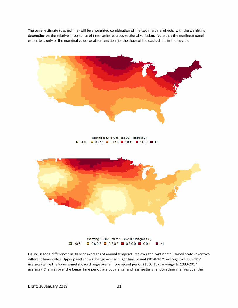
Figure 3 shows the variation in the change in 30-year averages of annual temperatures across the continental United States over two different timescales. The upper panel shows the longer timescale (1850-2017) which shows substantial spatial structure (associated with the amplification of warming at higher latitudes) that might be correlated with unobserved variables, introducing bias if used in a long-differences specification without regional fixed-effects or control variables. The lower panel shows changes over a shorter period of time (~50 years) and shows smaller, but more spatially heterogenous, changes. In general, the spatial pattern of variation in long differences will depend on the weather statistic (e.g. temperature will be different from rainfall) and the timescale under consideration.

One question around long differences is whether the variation used for the estimation reflects an actual change in the climate distribution or simply sampling variability that would be expected in a stochastic process. This question has not been dealt with explicitly in the literature, but has implications for the interpretation of long-differences estimates: would one expect to observe adaptation in response to fluctuations that may be consistent with a stationary climate distribution? In practice, this concern has been partly addressed either by demonstrating robustness of results to multiple start and end periods (e.g. 10-year averages vs 30-year averages) or by using fitted linear trends that capture long-term non-stationarity (Burke & Emerick, 2016; Moore & Lobell, 2015). It is important to note that, at the time and spatial scales examined in long-differences specifications so far, most of the variation used would not be expected to be a result of anthropogenic climate change. Instead it largely arises from low frequency natural variability in the climate system (Deser et al., 2012; Hawkins & Sutton, 2012).

Because long-differences uses a longer time-scale of variation than the inter-annual variation used in a standard panel model, it should capture the effect of adaptations that occur over the medium-term. If adaptations are available over decadal timescales that are not available over inter-annual timescales, then the marginal effect of a gradual change in weather will be less than the effect of a sudden change in weather. Referring back to Figure 1, this long-differences approach is estimating something in between the short- and long-run climate change effects. Depending on the rate of adaptation in the particular system, this might be closer to one or the other.

Dell, Jones and Olken (2012) use long-differences to estimate the effect of a one degree warming occurring over 15 years on GDP growth rates and find this is similar to the effect of interannual variations, arguing that this provides evidence that adaptation is not particularly effective over this time-frame. Burke and Emerick (2016) use long-differences (regressing the change in yield on the change in climate) to look at the effect of changes in temperature over a 20 year period on rainfed maize yields in the US and find effects similar to those estimated in a panel using interannual variation. Moore and Lobell (2015) and Lobell and Asner (2003) both also estimate the effect of decadal trends in temperature on yields in Europe and the US using specifications similar to long-differences.

With a long enough dataset, it is possible to develop a panel of long-differences by observing multiple periods of medium-term change in the same unit, improving the precision of the estimate of effects of changes at these time-scales and allowing for better control of unobserved variables. For example, Taraz (2017) develops a panel of decadal changes in the Indian monsoon to test for changes in irrigation


adoption and crop choice. Hsiang (2016) uses spectral analysis to create a panel of crop yield and temperature variation at various frequencies from 5 years to 33 years. He shows the estimated response of yield to temperature change is similar on all time-scales, suggesting limited effectiveness of adaptation.

3 Partitioning Variation

A final set of emerging approaches uses the fact that panel data contains variation in both weather and climate, and can therefore be used to jointly estimate the effects of both long- and short-run variation. We characterize these as “partitioning variation” because they decompose variation in the outcome variable into that associated with climate and that associated with interannual fluctuations around the climatological average. The former gives the long-run effect and the latter a short-run impact. A characteristic estimating equation involves economic value on the left hand side. The right hand side involves a nonlinear function of the weather deviation (from, for instance, a long-run mean), a nonlinear function of climate, controls and an error term. For instance, an estimating equation of this form is used by both Kelly et al (2005) and Moore and Lobell (2014) to jointly estimate the short- and long-run effect of warming on agriculture.

Despite using panel data, the long-run function of climate is estimated using cross-sectional variation. This means it is susceptible to the same set of omitted variable problems as the standard cross-section, and typically requires the inclusion of a large set of control variables. A possible alternative approach proposed by some authors is to use the fact that climate at a location varies over time to estimate both the long- and short-run effects in a panel, including location and period fixed effects.

This has the strong benefit of allowing for time-invariant omitted variables to be controlled for using the location fixed-effect. But it also changes the interpretation of the climate term – rather than the long-run equilibrium effect, it instead captures the medium-run effect. Depending on the timescale of adaptations, this may be closer to the long- or short-run response. Examples of this include Merel and Gammans (2017) as applied to US crop yields and Bento, Mookerjee, and Severnini (2017) who compare the effect of 30-year changes in mean ozone concentrations with that of inter-annual fluctuations around the mean.

One challenge of this approach is in knowing how to measure the long-term climate, particularly when the climate is non-stationary and given that we typically do not observe agents’ expectations of weather. If the estimated climate is different from what agents are actually expecting or prepared for, then this will induce measurement error into the deviation term and bias in the estimation of the short-run response. In practice, this appears not to matter substantively. For instance, Moore and Lobell (2014) use both a 30-year baseline climate and a 30-year rolling average to define climate and find it does not affect estimates of the short-run response.

One final, distinct, approach that shares theoretical commonalities with this set of studies, is to use forecast and unforecasted weather events to estimate the difference in response to surprising and expected weather. This approach uses the fact that reliable forecasts change actors’ information state, removing the gap between the short- and long-run response driven by imperfect information about the weather (Allen, Graff-Zivin, & Schrader, 2016; Schrader, 2017). In this sense, forecasted weather is analogous, in terms of the information available to actors, to a change in climate. Relatively few studies


have looked at forecasts in the context of climate change adaptation. Schrader (2017) uses the changing accuracy of El Nino forecasts to estimate the value of adaptation in the Pacific albacore fishery. Although not directly linked to climate change, Rosezweig and Udry (2014) show that Indian farmers adjust fertilizer application in response to skillful forecasts of monsoon intensity and show that accurate forecasts have significant value in this setting.

IV. RATES OF ADJUSTMENT AND ADAPTATION

The previous section has described the now rich and varied literature aimed at identifying the short-, medium-, and long-run effects of climate change. However, Figure 1 shows that fully identifying the total costs associated with climate change also requires determining the rate of adjustment. For a given adaptation effectiveness (i.e. difference between short- and long-run response curves), adjustment costs will be larger with a longer transition time. Kelly et al (2005) break down the rate of adaptation into two components: that associated with learning about a changed climate using weather observations and that associated with replacing long-lived capital and other quasi-fixed factors once learning has occurred.

Rates of adaptation are limited by learning if agents must infer a change in the underlying climate distribution using their own observations of weather, which provide only a noisy signal of the climate state. Kelly et al (2005) parameterize a Bayesian learning model based on characteristics of the climate system in order to estimate learning-related adjustment costs in US agriculture. Moore (2017) compares a hierarchical Bayesian learning model with simpler learning heuristics and shows that adjustment costs do not appear particularly sensitive to the learning model, so long as agents are able to learn from weather and update expectations about the climate distribution. Neither of these papers tests the hypothesized learning models against data. Kala (2016) however uses data on how planting dates respond to changes in the onset of the Indian monsoon to empirically compare several learning models, finding evidence for ambiguity aversion among farmers.

Even after accounting for learning-related adjustment costs, however, adaptation could be further slowed by the turnover time of long-lived capital (and possibly other factors of production which do not re-equilibrate instantaneously and costlessly). Since climate change is relatively gradual, it may be that capital will adjust gradually, however empirical studies are rare. Hornbeck (2012) shows that equilibrium adjustment to the Dust Bowl productivity shock took decades, suggesting that at least in some cases, the rate of adjustment could be comparable to the rate of climate change. Results of long-differences studies showing similar impacts of medium- and short-run changes in weather could be interpreted to suggest that either the potential for adaptation is small or that adaptation occurs only over longer time-scales (Burke & Emerick, 2016).

V. CONCLUSIONS

Improving the empirical basis for estimates of the economic consequences of climate change is important both as an area of academic inquiry and as an input into the formation of adaptation and mitigation policy decisions (Diaz & Moore, 2017). A long-standing (and by now well-worn) dichotomy has developed in the literature between cross-sectional and panel analysis for estimating climate change


impacts. On the one hand, cross-sectional analysis can be effective in capturing the long-run equilibrium impacts of different climates, at least in agriculture, but the threats to identification posed by omitted variables mean causal interpretation of results is not always warranted. On the other hand, panel regressions solve many omitted variable concerns through the use of location and time fixed-effects, but at the risk of only identifying the short-run response to weather variation, which will overestimate the impacts of climate change if adaptation is substantial.

The review presented here seeks to break through this dichotomy in two ways. Firstly, while much of the debate around cross-section vs panel regressions has focused on identifying the equilibrium costs of climate change, total damages are made up of both equilibrium and adjustment costs. The relative importance of these two components will depend on the speed and predictability of climate change and the dynamics of capital adjustment in a particular sector. Neither cross-sections nor standard panel models alone identify both types of costs.

Secondly, our review of new methods being applied to panel data (termed “hybrid approaches” in this paper) reveal it is not always the case that using panel data, even with location fixed-effects, limits identification to only the short-run response. Panel data contains rich information on the effects of short-, medium-, and long-term variation in weather, and new approaches are using this in innovative ways to estimate the response functions on multiple timescales. These approaches greatly reduce omitted variable concerns relative to a cross-section while still estimating a response that includes more adaptation than occurs in response to interannual variation in weather. This remains fertile ground for research; judging by the number of new and innovative working papers being produced, this is recognized by the research community.

This review has also uncovered a number of pressing research needs. These include better integration of new empirical approaches with theoretical models describing the dynamic response of agents to a changing climate, as well as more work to constrain the rate of adaptation in various locations and sectors. Furthermore, while much empirical work has focused on the US and particularly in the agriculture sector, expansion beyond these settings is desirable for fully understanding the effects of climate change.

This is an exciting, important, promising and active field of research.


Table I: Summary of different empirical approaches to estimating impacts of weather and climate on economic activity.

Approach Stylized Estimating Equation Typical Representation of Weather

Typical Representation of Climate

Remarks Selected Papers

Cross-Section 𝑦𝑦𝑖𝑖 = 𝑓𝑓(𝑐𝑐𝑖𝑖) + 𝐶𝐶𝐶𝐶𝐶𝐶𝐶𝐶𝐶𝐶𝐶𝐶𝐶𝐶𝐶𝐶𝑖𝑖 + 𝜀𝜀𝑖𝑖 None Direct and Nonlinear

Applies at a single time point

Mendelsohn et al (1994)

Linear Panel 𝑦𝑦𝑖𝑖𝑖𝑖 = 𝛽𝛽𝑤𝑤𝑖𝑖𝑖𝑖 + 𝜇𝜇𝑖𝑖 + 𝜃𝜃𝑖𝑖 + 𝜀𝜀𝑖𝑖𝑖𝑖 Linear Removed through fixed effects

Deschenes and Greenstone (2007)

Dell, Jones and Olken (2012)

Heterogeneous Marginal Effects: Nonlinear Panel

𝑦𝑦𝑖𝑖𝑖𝑖 = 𝑓𝑓(𝑤𝑤𝑖𝑖𝑖𝑖) + 𝜇𝜇𝑖𝑖 + 𝜃𝜃𝑖𝑖 + 𝜀𝜀𝑖𝑖𝑖𝑖 Non-linear Removed through fixed effects. Marginal effect of weather varies with climate.

Deryugina and Hsiang (2017)

Burke, Hsiang, and Miguel (2015)

Heterogeneous Marginal Effects: Two Stage Panel

1st𝑦𝑦𝑖𝑖𝑖𝑖 = 𝛽𝛽𝑖𝑖𝑤𝑤𝑖𝑖𝑖𝑖 + 𝜇𝜇𝑖𝑖 + 𝜃𝜃𝑖𝑖 + 𝜀𝜀𝑖𝑖𝑖𝑖

2nd𝛽𝛽𝑖𝑖 = 𝑓𝑓(𝑐𝑐𝑖𝑖) + 𝐶𝐶𝐶𝐶𝐶𝐶𝐶𝐶𝐶𝐶𝐶𝐶𝐶𝐶𝐶𝐶𝑖𝑖 + 𝜀𝜀𝑖𝑖

Linear in first stage; absent in second stage

Fixed effects in first stage;

direct nonlinear in second stage

Coefficient on weather in first stage becomes LHS in stage 2

Butler and Huybers (2012); Heutel et al (2017)

Auffhammer (2018)

Long Differences 𝑦𝑦𝑖𝑖,𝑖𝑖 − 𝑦𝑦𝑖𝑖,𝑖𝑖−∆𝑖𝑖 =

𝑓𝑓�𝑤𝑤𝑖𝑖,𝑖𝑖 − 𝑤𝑤𝑖𝑖,𝑖𝑖−∆𝑖𝑖�+ 𝜀𝜀𝑖𝑖

Linear Medium-run climatic variation captured through long differences

Burke and Emerick (2016); Moore and Lobell (2015)

Partitioning Variation

𝑦𝑦𝑖𝑖𝑖𝑖 = 𝑓𝑓(𝑤𝑤𝑖𝑖𝑖𝑖 − 𝑐𝑐𝑖𝑖) + 𝑔𝑔(𝑐𝑐𝑖𝑖)

+𝐶𝐶𝐶𝐶𝐶𝐶𝐶𝐶𝐶𝐶𝐶𝐶𝐶𝐶𝐶𝐶𝑖𝑖 + 𝜀𝜀𝑖𝑖𝑖𝑖

Nonlinear Nonlinear Kelly et al (2005)

Moore and Lobell (2014)


Key: In equations, y represents the value of economic activity, w represents a weather statistic, c represents the climate (ie, the distribution of the weather statistic), i is an index on spatial location, t is an index on time, μ is a fixed effect varying with time, θ is a fixed effect varying over space, ε is an error term and “controls” refers to other relevant exogenous variables. β is a coefficient to be estimated and f() is a nonlinear function, also to be estimated.


Figure One: Components of welfare losses under sudden and gradual climate change. a) Mean temperature for a sudden change in climate. b) Equilibrium and adjustment costs given a sudden change in climate. c) Mean temperature for a gradual change in climate. d) Equilibrium and adjustment costs given a gradual change in climate. Adapted from Kelly, Kolstad and Mitchell (2005).


Figure 2: Schematic example of panel estimates with heterogeneous marginal effects of weather. There are two locations (red and blue), with a uni-dimensional weather (eg temperature). Climate (weather distributions) are shown in the shaded areas, and two production technologies are shown by the solid lines. In the upper panel, the weather at the two locations is quite different, with no overlap between the two distributions. In the lower panel the two locations are more similar. The warmer location (red) uses the production technology that is less sensitive to extreme heat while the cooler location (blue) uses the technology that performs better at cooler temperatures.


The panel estimate (dashed line) will be a weighted combination of the two marginal effects, with the weighting depending on the relative importance of time-series vs cross-sectional variation. Note that the nonlinear panel estimate is only of the marginal value-weather function (ie, the slope of the dashed line in the figure).

Figure 3: Long-differences in 30-year averages of annual temperatures over the continental United States over two different time-scales. Upper panel shows change over a longer time period (1850-1879 average to 1988-2017 average) while the lower panel shows change over a more recent period (1950-1979 average to 1988-2017 average). Changes over the longer time period are both larger and less spatially random than changes over the


shorter time period. Values shown are spatial averages over US counties of temperature data on a 1° grid interpolated from station data by Berkeley Earth. 10

10 Berkeley Earth Data. Retrieved March 5, 2018, from http://berkeleyearth.org/data/


References

Abel AB, and JC Eberly (1994). “A Unified Model of Investment Under Uncertainty,” Amer Econ Rev, 84:1369-85.

Allen, R., Graff-Zivin, J., & Schrader, J. (2016). Forecasting in the Presence of Expectations. European Physical Journal Special Topics, 225(3), 535–550.

Arguez, A., & Vose, R. S. (2011). The Key to Deriving Alternative Climate normals. Bulletin of the American Meteorological Society, 92(6), 699–704. http://doi.org/10.1175/2010BAMS2955.1

Auffhammer, M. (2018). Climate Adaptive Response Estimation: Short and Long Run Impacts of Climate Change on Residential Electricity and Natural Gas Consumption Using Big Data (No. 24397). Cambridge, MA.

Barreca, A., Clay, K., Deschênes, O., Greenstone, M., & Shapiro, J. S. (2015). Convergence in Adaptation to Climate Change: Evidence from High Temperatures and Mortality, 1900–2004. American Economic Review, 105(5), 247–251. http://doi.org/10.1257/aer.p20151028

Blanc, Elodie and Wolfram Schlenker, "The Use of Panel Models in Assessment of Climate Impacts on Agriculture," Rev. Env. Econ. Pol., 11:258-79 (2017).

Burke, M. B., & Emerick, K. (2016). Adaptation to Climate Change: Evidence from U.S. Agriculture. American Economic Journal: Economic Policy, 8(3), 108–140. Retrieved from http://web.stanford.edu/~mburke/papers/Burke_Emerick_2015.pdf

Burke, M., Craxton, M., Kolstad, C. D., Onda, C., Allcott, H., Baker, E., … Tol, R. S. J. (2016). Opportunities for advances in climate change economics. Science, 352(6283), 292–293. Retrieved from http://science.sciencemag.org/content/352/6283/292.abstract

Burke, M., Hsiang, S. M., & Miguel, E. (2015). Global non-linear effect of temperature on economic production. Nature, 527, 235–239. http://doi.org/10.1038/nature15725

Butler, E. E., & Huybers, P. (2012). Adaptation of US maize to temperature variations. Nature Climate Change, 3(1), 68–72. http://doi.org/10.1038/nclimate1585

Carleton, T. A., & Hsiang, S. M. (2016). Social and economic impacts of climate. Science, 353(6304), 1112. http://doi.org/10.1126/science.aad9837

Carleton TA, et al. (2018) Valuing the Global Mortality Consequences of Climate Change Accounting for Adaptation Costs and Benefits (Becker Friedman Institute, Working Paper No 2018-51, Chicago, IL).

Dell, B. M., Jones, B. F., & Olken, B. A. (2012). Temperature Shocks and Economic Growth: Evidence from the Last Half Century. American Economic Journal: Macroeconomics, 4(3), 66–95.

Dell, M., Jones, B. F., & Olken, B. A. (2014). What Do We Learn from the Weather? The New Climate-Economy Literature. Journal of Economic Literature.

Deryugina, T., & Hsiang, S. M. (2017). The Marginal Product of Climate (NBER Working Paper Series No. 24072). Cambridge, MA.

Deschênes, O., & Greenstone, M. (2007). The Economic Impacts of Climate Change: Evidence from Agricultural Output and Random Fluctuations in Weather. American Economic Review, 97(1), 354–385. http://doi.org/10.1257/aer.97.1.354


Deser, C., Knutti, R., Solomon, S., & Phillips, A. S. (2012). Communication of the Role of Natural Variability in Future North American Climate. Nature Climate Change, 2(October), 775–780. http://doi.org/10.1038/NCLIMATE1562

Diaz, D., & Moore, F. C. (2017). Quantifying the Economic Risks of Climate Change. Nature Climate Change, 7, 774–782.

Fischer, E. M., & Knutti, R. (2013). Robust Projections of Combined Humidity and Temperature Extremes. Nature Climate Change, 3, 126–130.

Guo, C., & Costello, C. (2013). The value of adaption: Climate change and timberland management. Journal of Environmental Economics and Management, 65(3), 452–468. http://doi.org/10.1016/j.jeem.2012.12.003

Hawkins, E., & Sutton, R. (2012). Time of Emergence of Climate Signals. Geophysical Research Letters, 39(1), L01702. http://doi.org/10.1029/2011GL050087

Heutel, G., Miller, N. H., & Molitor, D. (2017). Adaptation and Mortality Effects of Temperature Across U.S. Climate Regions (NBER Working Paper No. 23271). Cambridge, MA.

Hornbeck, R. (2012). The Enduring Impact of the American Dust Bowl: Short and Long-Run Adjustments to Environmental Catastrophe. American Economic Review, 102(4), 1477–1507.

Hsiang S. M. & Burke M. (2014) Climate, conflict, and social stability: what does the evidence say? Clim Change 123(1):39–55.

Hsiang, S. M. (2016). Climate Econometrics. Annual Review of Resource Economics, 8, 43–75.

Kelly, D., Kolstad, C., & Mitchell, G. (2005). Adjustment Costs from Environmental Change. Journal of Environmental Economics and Management, 50(3), 468–495. http://doi.org/10.1016/j.jeem.2005.02.003

Lemoine (2018) Sufficient Statistics for the Cost of Climate Change (NBER Working Paper No. 25008). Cambridge, MA.

Lobell, D. B., & Asner, G. P. (2003). Climate and Management Contributions to Recent Trends in U.S. Agricultural Yields. Science, 299, 1032.

Massetti E. & Mendelsohn R. (2011) Estimating Ricardian Functions with Panel Data. Clim Chang Econ 2:301–319.

Mendelsohn, R. (2000). Efficient Adaptation to Climate Change. Climatic Change, 45, 583–600.

Mendelsohn, R., Nordhaus, W. D., & Shaw, D. (1994). The Impact of Global Warming on Agriculture: A Ricardian Analysis. American Economic Review, 84(4), 753–771.

Mendelsohn, R., & Reinsborough, M. (2007). A Ricardian analysis of US and Canadian farmland. Climatic Change, 81(1), 9–17. http://doi.org/10.1007/s10584-006-9138-y

Moore, F. C. (2017). Learning, Adaptation, and Weather in a Changing Climate. Climate Change Economics, 8(4), 1750010–1.

Moore, F. C., & Lobell, D. B. (2014). The Adaptation Potential of European Agriculture in Response to Climate Change. Nature Climate Change, 4(7), 610–614.


Moore, F. C., & Lobell, D. B. (2015). The Fingerprint of Climate Trends on European Crop Yields. Proceedings of the National Academy of Sciences, 11(9), 2670–2675. http://doi.org/10.1073/pnas.1409606112

Ortiz-Bobea, A. (2016). The Economic Impacts of Climate Change on Agriculture: Accounting for Time-Invariant Unobservables in the Hedonic Approach. Dyson School of Applied Economics and Management Working Paper (No 2016-15), Ithaca, NY.

Quiggin, J., & Horowitz, J. K. (1999). The Impact of Global Warming on Agriculture: A Ricardian Analysis: Comment. American Economic Review, 89(4), 1044–1045.

Rosenzweig, M., & Udry, C. R. (2014). Forecasting Profitability (No. 19334). Cambridge, MA.

Schlenker, W. (2010). Crop Responses to Climate and Weather: Cross-Section and Panel Models. In D. B. Lobell & M. B. Burke (Eds.), Climate Change and Agriculture: Adapting Agriculture to a Warmer World (pp. 99–108). Amsterdam: Springer Netherlands.

Schlenker, W., Hanemann, W. M., & Fischer, A. C. (2005). Will U.S. Agriculture Really Benefit from Global Warming? Accounting for Irrigation in the Hedonic Approach. American Economic Review, 95(1), 395–406.

Schlenker W., Hanemann W. M., Fisher A. C. (2006) The Impact of Global Warming on U.S. Agriculture: An Econometric Analysis of Optimal Growing Conditions. Rev Econ Stat 88(1):113–125.

Schlenker, W., & Roberts, D. L. (2009). Nonlinear Temperature Effects Indicate Severe Damages to U.S. Corn Yields Under Climate Change. Proceedings of the National Academy of Sciences, 106(37), 15594–15598.

Schlenker, W., Roberts, M. J., & Lobell, D. B. (2013). US maize adaptability. Nature Climate Change, 3(8), 690–691. http://doi.org/10.1038/nclimate1959

Severen, C., Costello, C., & Deschênes, O. (2016). A Forward Looking Ricardian Approach: Do Land Markets Capitalize Climate Change Forecasts? (NBER Working Paper No. 22413). Cambridge, MA.

Taraz, V. (2017). Adaptation to Climate Change: Historical Evidence from the Indian Monsoon. Environment and Development Economics, 22(5), 517–545.

Thompson, D. W. J., Barnes, E. A., Deser, C., Foust, W., & Philips, A. S. (2015). Quantifying the Role of Internal Climate Variability in Future Climate Trends. Journal of Climate. http://doi.org/10.1175/JCLI-D-14-00830.1

estimating the economic impacts of climate change using

Documents