estimating the jacobian of the singular value

HAL Id: inria-00072686https://hal.inria.fr/inria-00072686

Submitted on 24 May 2006

HAL is a multi-disciplinary open accessarchive for the deposit and dissemination of sci-entific research documents, whether they are pub-lished or not. The documents may come fromteaching and research institutions in France orabroad, or from public or private research centers.

L’archive ouverte pluridisciplinaire HAL, estdestinée au dépôt et à la diffusion de documentsscientifiques de niveau recherche, publiés ou non,émanant des établissements d’enseignement et derecherche français ou étrangers, des laboratoirespublics ou privés.

Estimating the Jacobian of the Singular ValueDecomposition : Theory and Applications

Théodore Papadopoulo, Manolis L.A. Lourakis

To cite this version:Théodore Papadopoulo, Manolis L.A. Lourakis. Estimating the Jacobian of the Singular Value Decom-position : Theory and Applications. [Research Report] RR-3961, INRIA. 2000, pp.21. �inria-00072686�

https://hal.inria.fr/inria-00072686

https://hal.archives-ouvertes.fr

ISS

N 0

249-

6399

ISR

N IN

RIA

/RR

--39

61--

FR

+E

NG

ap por t de r ech er ch e

THÈME 3

INSTITUT NATIONAL DE RECHERCHE EN INFORMATIQUE ET EN AUTOMATIQUE

Estimating the Jacobian of the Singular ValueDecomposition: Theory and Applications

Théodore PAPADOPOULO and Manolis I.A. LOURAKIS

N° 3961

Juin 2000

Unité de recherche INRIA Sophia Antipolis2004, route des Lucioles, B.P. 93, 06902 Sophia Antipolis Cedex (France)

Téléphone : 04 92 38 77 77 - International : +33 4 92 38 77 77 — Fax : 04 92 38 77 65 - International : +33 4 92 38 77 65

Estimating the Jacobian of the Singular Value Decomposition:Theory and Applications

Théodore PAPADOPOULO and Manolis I.A. LOURAKIS

Thème 3 — Interaction homme-machine,images, données, connaissances

Projet Robotvis

Rapport de recherche n° 3961 — Juin 2000 — 21 pages

Abstract: The Singular Value Decomposition (SVD) of a matrix is a linear algebra tool that hasbeen successfully applied to a wide variety of domains. The present paper is concerned with theproblem of estimating the Jacobian of the SVD components of a matrix with respect to the matrixitself. An exact analytic technique is developed that facilitates the estimation of the Jacobian usingcalculations based on simple linear algebra. Knowledge of the Jacobian of the SVD is very useful incertain applications involving multivariate regression or the computation of the uncertainty relatedto estimates obtained through the SVD. The usefulness and generality of the proposed technique isdemonstrated by applying it to the estimation of the uncertainty for three different vision problems,namely self-calibration, epipole computation and rigid motion estimation.

Key-words: Singular Value Decomposition, Jacobian, Uncertainty, Calibration, Structure fromMotion.

M. Lourakis was supported by the VIRGO research network (EC Contract No ERBFMRX-CT96-0049) of theTMR Programme.

Calcul de la Jacobienne de la Décomposition en ValeursSingulières: Théorie et applications

Résumé : La technique de Décomposition en Valeurs Singulières (SVD) d’une matrice est unoutil algèbrique qui a trouvé de nombreuses applications en vision par ordinateur. Dans ce rapport,nous nous intéressons au problème de l’estimation de la jacobienne de la SVD par rapport auxcoefficients de la matrice initiale. Cette jacobienne est très utile pour toute une gamme d’applicationsfaisant intervenir des estimations aux moindres carrés (pour lesquelles on utilise la SVD) ou bien descalculs d’incertitude pour des grandeurs estimées de cette manière. Une solution analytique simpleà ce problème est présentée. Elle exprime la jacobienne à partir de la SVD de la matrice à l’aided’opérations très simples d’algèbre linéaire. L’utilité et la généralité de la technique est démontréeen l’appliquant à trois problèmes de vision: l’auto-calibration, le calcul d’épipoles et l’estimation demouvements rigides.

Mots-clés : Décomposition en valeurs singulières, Jacobienne, Incertitude, Calibration, Structureà partir du mouvement.

Estimating the Jacobian of the Singular Value Decomposition: Theory and Applications 3

1 Introduction and Motivation

The SVD is a general linear algebra technique that is of utmost importance for several computationsinvolving matrices. For example, some of the uses of SVD include its application to solving ordinaryand generalized least squares problems, computing the pseudo-inverse of a matrix, assessing thesensitivity of linear systems, determining the numerical rank of a matrix, carrying out multivariateanalysis and performing operations such as rotation, intersection, and distance determination onlinear subspaces [10]. Owing to its power and flexibility, the SVD has been successfully applied toa wide variety of domains, from which a few sample applications are briefly described next.

Zhang et al [46], for example, employ the SVD to develop a fast image correlation scheme. Theproblem of establishing correspondences is also addressed by Jones and Malik [15], who comparefeature vectors defined by the responses of several spatial filters and use the SVD to determine thedegree to which the chosen filters are independent of each other. Structure from motion is anotherapplication area that has greately benefited from the SVD. Longuet-Higgins [20] and later Hartley[11] extract the translational and rotational components of rigid 3D motion using the SVD of theessential matrix. Tsai et al [40] also use the SVD to recover the rigid motion of a 3D planar patch.Kanade and co-workers [39, 31, 29] assume special image formation models and use the SVD tofactorize image displacements to structure and motion components. Using an SVD based method,Sturm and Triggs [38] recover projective structure and motion from uncalibrated images and thusextend the work of [39, 31] to the case of perspective projection. The SVD of the fundamentalmatrix yields a simplified form of the Kruppa equations, on which self-calibration is based [12,21, 22]. Additionally, the SVD is used to deal with important image processing problems such asnoise estimation [16], image coding [44] and image watermarking [19]. Several parametric fittingproblems involving linear least squares estimation, can also be effectively resolved with the aid ofthe SVD [2, 41, 17]. Finally, the latter has also proven useful in signal processing applications[35, 28] and pattern recognition techniques such as neural networks computing [7, 43] and principalcomponents analysis [4].

This paper deals with the problem of computing the Jacobian of the SVD components of a matrixwith respect to the elements of this matrix. Knowledge of this Jacobian is important as it is a keyingredient in tasks such as non-linear optimization and error propagation:

• Several optimization methods require that the Jacobian of the criterion that is to be optimized isknown. This is especially true in the case of complicated criteria. When these criteria involvethe SVD, the method proposed in this paper is invaluable for providing analytical estimates oftheir Jacobians. As will be further explained latter, numerical computation of such Jacobiansusing finite differences is not as straightforward as it might seem at a first glance.

• Computation of the covariance matrix corresponding to some estimated quantity requiresknowledge of the Jacobians of all functions involved in the estimation of the quantity in ques-tion. Considering that the SVD is quite common in many estimation problems in vision, themethod proposed in this work can be used in these cases for computing the covariance matricesassociated with the estimated objects.

RR n° 3961

4 Théodore PAPADOPOULO and Manolis I.A. LOURAKIS

Paradoxically, the numerical analysis litterature provides little help on this topic. Indeed, a lotof studies have been made on the sensitivity of singular values and singular vectors to perturbationsin the original matrix [37, 10, 6, 42, 3], but these globally consider the question of perturbing theinput matrix and derive bounds for the singular elements but do not deal with perturbations due toindividual elements.

The method proposed is an extension to non-singular matrices of the method proposed in [26].This method seems not to be of widespread use, particularly in the conputer vision field. In a firstsection, we present the method for computing SVD differentiation and describe its properties.

The rest of this paper is organized as follows. Section 2 gives an analytical derivation for thecomputation of the Jacobian of the SVD and discusses practical issues related to its implementationin degenerate cases. Section 3 illustrates the use of the proposed technique with three examples ofcovariance matrix estimation. The paper concludes with a brief discussion in section 4.

2 The Proposed Method

2.1 Notation and Background

In the rest of the paper, bold letters will be used for denoting vector and matrices. The transpose ofmatrix

�is denoted by

��and �� refers to the �� element of

�. The -th non-zero element

of a diagonal matrix � is referred to by �� , while� � designates the -th column of matrix

�.

A basic theorem of linear algebra states that any real �� matrix � with � �� can bewritten as the product of an �� column orthogonal matrix � , an �� diagonal matrix �with non-negative diagonal elements (known as the singular values), and the transpose of an �� orthogonal matrix ! [10]. In other words,

��"#�$�%! � "&'�)(+*�,�-�.�/! ��10 (1)

The singular values are the square roots of the eigenvalues of the matrix �.� � (or � � � sincethese matrices share the same non-zero eigenvalues) while the columns of � and ! (the singularvectors) correspond to the eigenvectors of �.� � and � � � respectively [18]. As defined in Eq.(1),the SVD is not unique since

• it is invariant to arbitrary permutations of the singular values and their corresponding left andright singular vectors. Sorting the singular values (usually by decreasing magnitude order)solves this problem unless there exist equal singular values.

• simultaneous changes in the signs of the vectors � � and ! � do not have any impact on the left-most part of Eq.(1). In practice, this has no impact on most numerical computations involvingthe SVD.

INRIA


2.2 Computing the Jacobian of the SVD

Employing the definitions of section 2.1, we are interested in computing � �� , � �� and � �� forevery element �� of the � � � matrix � .Taking the derivative of Eq. (1) with respect to �� yields the following equation

� � � " � �� %! ��

� � � ! �� ! � �

�(2)

Clearly, �� -��" �� "�� , while � � �� "�� . Since � is an orthogonal matrix, we have thefollowing:

� � � "�� "�� "! � �� "!" � (3)

where �� is given by

� �� "#� � � �� 0 (4)

From Eq. (3) it is clear that �� is an antisymmetric matrix. Similarly, an antisymmetric matrix � ��can be defined for ! as

� �� " ! � ��! 0 (5)

Notice that �� and � �� are specific to each differentiation �� .

By multiplying Eq. (2) by � � and ! from the left and right respectively, and using Eqs. (4) and(5), the following relation is obtained:

� � � �� ! "# �� 0 (6)

Since �� and �� are antisymmetric matrices, all their diagonal elements are equal to zero.Recalling that � is a diagonal matrix, it is easy to see that the diagonal elements of �� and �$ � ��are also zero. Thus, Eq. (6) yields the derivatives of the singular values as �&% � � "(' �)%+* �,% 0 (7)

Taking into account the antisymmetry property, the elements of the matrices �� and �� can becomputed by solving a set of - �.- linear systems, which are derived from the off-diagonal elementsof the matrices in Eq. (6): / �102 � �� % 0 � � % � �� % 0 " ' �3% * � 0

�4%5 � �� % 0 � � 0 � �� % 0 "76 ' � 0 * �,%�� (8)

RR n° 3961


where the index ranges are � " � 0 0 0 � and � "� � � 0 0 0 � . Note that, since the � % are positivenumbers, this system has a unique solution provided that � % �" �40 . Assuming for the moment that �� ,�-� � � % �"��40 , the

& � &�� *�� parameters defining the non-zero elements of � �� and � �� can be

easily recovered by solving the& � &�� *�� corresponding -%� - linear systems.

Once � �� and �� have been computed, � �� and � �� follow as:

� �� " �$ � �� ! �� "76 !� � �� 0 (9)

In summary, the desired derivatives are supplied by Eqs. (7) and (9).

2.3 Implementation and Practical Issues

In this section, a few implementation issues related to a practical application of the proposed methodare considered.

2.3.1 Degenerate SVDs.

Until now, the case where the SVD yields at least two identical singular values has been set aside.However, such cases occur often in practice, for example when dealing with the essential matrix(see section 3.3 ahead) or when fitting a line in 3D. Therefore, let us now assume that � % "�� 0 forsome � and � . It is easy to see that these two singular values contribute to Eq. (1) with the term� 0 ��% ! �% � � 0 ! �0�� . The same contribution to � can be obtained by using any other orthonormalbases of the subspaces spanned by �� %�� 0 � and �! %�� ! 0 � respectively. Therefore, letting

�� % " �� % � � �� $0�� 0 "76�� % � �� 0!� % " �� !�% � � �� ! 0!� 0 "76�� !�% � �� ! 0 �

for any real number � , we have � % ! �% � � 0 ! �0 " � % ! % � � � 0 ! 0 � . This implies that in thiscase, there exists a one dimensional family of SVDs. Consequently, the -$� - system of Eqs. (8)must be solved in a least squares fashion in order to get only the component of the Jacobian that is“orthogonal” to this family. Of course, when more than two singular values are equal, all the - � -corresponding systems have to be solved simultaneously. The correct algorithm for all cases is thus:

• Group together all the -%� - systems corresponding to equal singular values.

• Solve these systems using least squares.

This will give the exact Jacobian in non-degenerate cases and the “minimum norm” Jacobian whenone or more singular values are equal.

INRIA


2.3.2 Computational complexity.

Assuming that the matrix � is � � � and non-degenerate for simplicity, it is easy to compute thecomplexity of the procedure for computing the Jacobian: For each pair �/�� " � 0 0 0 � � " � � 0 0 0 � , a total of

& � &�� *�� - ��- linear systems have to be solved. In essence, the complexity ofthe method is �%�� once the initial SVD has been carried out.

2.3.3 Computing the Jacobian using finite differences.

The proposed method has been compared with a finite difference approximation of the Jacobian andsame results have been obtained in the non-degenerate case (degenerate cases are more difficult tocompare due to the non-uniqueness of the SVD). Although the ease of implementation makes thefinite difference approximation more appealing for computing the Jacobian, the following pointsshould also be taken into account:

• The finite difference method is more costly in terms of computational complexity. Consideringagain the case of an � � � non-degenerate matrix as in the previous paragraph, it is simpleto see that such an approach requires � � SVD computations to be performed (i.e. one foreach perturbation of each element of the matrix). Since the complexity of the SVD operationis �%�/�� , the overall complexity of the approach is �%�/�� which is an order of magnitudehigher compared to that corresponding to the proposed method.

• Actually, the implementation of a finite difference approximation to a Jacobian is not as simpleas it might appear. This is because even state of the art algorithms for SVD computation (egLAPACK’s dgesvd family of routines [1]) are “unstable” with respect to small perturbations ofthe input. By unstable, we mean that the signs associated with the columns � � and ! � canchange arbitrarily even with the slightest perturbation. In general, this is not important butit has strong effects in our case since the original and perturbed SVD do not return the sameobjects. Consequently, care has to be taken to compensate for this effect when the Jacobian iscomputed through finite differences.

3 Applications

In this section, the usefulness and generality of the proposed SVD differentiation method are demon-strated by applying it to three important vision problems. Before proceeding to the description ofeach of these problems, we briefly state a theorem related to error propagation that is essential forthe developments in the subsections that follow. More specifically, let �� & be a measurementvector, from which a vector �� is computed through a � * function � , i.e. �� "�� . Here,we are interested in determining the uncertainty of �� , given the uncertainty of �� . Let �� & bea random vector with mean �� and covariance �� "�� 6�� 6!�� "

. The vector �"�� is also random and its covariance ��# up to first order is equal to

� # " � �� $�

� �� (10)

RR n° 3961


where �� is the derivative of � at �� . For more details and proof, the reader is referred to [8]. Inthe following, Eq. (10) will be used for computing the uncertainty pertaining to various entities thatare estimated from images. Since image measurements are always corrupted by noise, the estimationof the uncertainty related to these entities is essential for effectively and correctly employing thelatter in subsequent computations.

3.1 Self-Calibration Using the SVD of the Fundamental Matrix

The first application that we deal with is that of self-calibration, that is the estimation of the cam-era intrinsic parameters without relying upon the existence of a calibration object. Instead, self-calibration employs constraints known as the Kruppa equations, which are derived by tracking im-age features through an image sequence. More details regarding self-calibration can be found in[27, 45, 24, 21, 22]. Here, we restrict our attention to a self-calibration method that is based ona simplification of the Kruppa equations derived from the SVD of the fundamental matrix. In thefollowing paragraph, a brief description of the method is given; more details can be found in [21, 23].

Let��

be the vector formed by the parameters of the SVD of the fundamental matrix � . TheKruppa equations in this case reduce to three linearly dependent constraints, two of which are lin-early independent. Let � � � � � �� " � 0 0 0�� denote those three equations as functions of thefundamental matrix � and the matrix " �.� � , where � is the � � � intrinsic calibration para-meters matrix having the following well-known form [8]:

� " � �� 6�� '�� ! #"$� *��

%&(11)

The parameters �� and �� correspond to the focal distances in pixels along the axes of the image,� is the angle between the two image axes and � ''� ��*�� are the coordinates of the image principalpoint. In practice, � is very close to ( � for real cameras. The matrix is parameterized with theunknown intrinsic parameters from Eq.(11) and is computed from the solution of a non-linear leastsquares problem, namely

"(*),+ �$��.-/ &'� ( *

� �* � �'� � �'0��1 �(32 � �� 0 �� '� � �'0��1 �(34 � �� 0 �

� � �� 0��1 �(,5 � �'� � � 0 � (12)

In the above equation, � is the number of the available fundamental matrices and 1 �( � � �� arethe variances of constraints � � � �'� �� 1" � 0 0 0�� , respectively, used to automatically weight theconstraints according to their uncertainty. It is to the estimation of these variances that the proposeddifferentiation method is applied. More specifically, applying Eq.(10) to the case of the simplifiedKruppa equations, it is straightforward to show that the variance of the latter is approximated by

1 �( � � �� " � � � �'� �6��

� � � � �'� �6��

In the above equation, � ( � �87*9;: / �� 7*9 is the derivative of � � � �'� �6�� at�'�

, � 7*9� � is the Jacobian of��

at � and � �is the covariance of the fundamental matrix, supplied as a by-product of the procedure

INRIA


for estimating � [5]. The derivative � ( � �87*9;: / �� 7 9 is computed directly from the analytic expression for� � � �'� �6�� , while � 7 9� � is estimated using the proposed method for SVD differentiation.

0

1

2

3

4

5

6

7

8

0 0.5 1 1.5 2 2.5 3 3.5 4

Mea

n a_

u re

lativ

e er

ror

(%)

Noise standard deviation (pixels)

Mean a_u relative error vs. noise standard deviation

with covwithout cov

0

1

2

3

4

5

6

7

8

9

0 0.5 1 1.5 2 2.5 3 3.5 4

Mea

n a_

v re

lativ

e er

ror

(%)


Mean a_v relative error vs. noise standard deviation

with covwithout cov

0

1

2

3

4

5

6

7

8

0 0.5 1 1.5 2 2.5 3 3.5 4

Std

dev

iatio

n of

a_u

rel

ativ

e er

ror

(%)


Std deviation of a_u relative error vs. noise standard deviation

with covwithout cov

0

1

2

3

4

5

6

7

8

9

10

11

0 0.5 1 1.5 2 2.5 3 3.5 4

Std

dev

iatio

n of

a_v

rel

ativ

e er

ror

(%)


Std deviation of a_v relative error vs. noise standard deviation

with covwithout cov

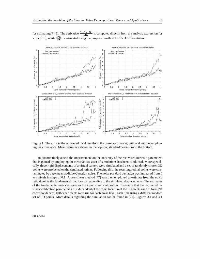
Figure 1: The error in the recovered focal lengths in the presence of noise, with and without employ-ing the covariance. Mean values are shown in the top row, standard deviations in the bottom.

To quantitatively assess the improvement on the accuracy of the recovered intrinsic parametersthat is gained by employing the covariances, a set of simulations has been conducted. More specifi-cally, three rigid displacements of a virtual camera were simulated and a set of randomly chosen 3Dpoints were projected on the simulated retinas. Following this, the resulting retinal points were con-taminated by zero mean additive Gaussian noise. The noise standard deviation was increased from 0to 4 pixels in steps of 0.1. A non-linear method [47] was then employed to estimate from the noisyretinal points the fundamental matrices corresponding to the simulated displacements. The estimatesof the fundamental matrices serve as the input to self-calibration. To ensure that the recovered in-trinsic calibration parameters are independent of the exact location of the 3D points used to form 2Dcorrespondences, 100 experiments were run for each noise level, each time using a different randomset of 3D points. More details regarding the simulation can be found in [21]. Figures 3.1 and 3.1

RR n° 3961


illustrate the mean and standard deviation of the relative error for the intrinsic parameters versus thestandard deviation of the noise added to image points, with and without employing the covariances.When the covariances are not employed, the weights 1 �( � � �� 0�� in Eq.(12) are all assumed to beequal to one. Throughout all experiments, zero skew has been assumed, i.e. � " �� - and 0 inEq. (12) was parameterized using 4 unknowns. As is evident from the plots, especially those refer-ring to the standard deviation of the relative error, the inclusion of covariances yields more accurateand more stable estimates of the intrinsic calibration parameters. Additional experimental resultscan be found in [21]. At this point, it is also worth mentioning that in the case of self-calibration, thederivatives � 7 9� � were also computed analytically by using MAPLE to compute closed-form expres-sions for the SVD components with respect to the elements of � . Using the computed expressions forthe SVD, the derivative of the latter with respect to � was then computed analytically. As expected,the arithmetic values of the derivatives obtained in this manner were identical to those computed bythe differentiation method proposed here.

0

2

4

6

8

10

12

14

16

18

20

22

0 0.5 1 1.5 2 2.5 3 3.5 4

Mea

n u_

0 re

lativ

e er

ror

(%)


Mean u_0 relative error vs. noise standard deviation

with covwithout cov

0

2

4

6

8

10

12

14

16

18

20

0 0.5 1 1.5 2 2.5 3 3.5 4

Mea

n v_

0 re

lativ

e er

ror

(%)


Mean v_0 relative error vs. noise standard deviation

with covwithout cov

0

4

8

12

16

20

24

28

32

36

40

44

0 0.5 1 1.5 2 2.5 3 3.5 4

Std

dev

iatio

n of

u_0

rel

ativ

e er

ror

(%)


Std deviation of u_0 relative error vs. noise standard deviation

with covwithout cov

0

2

4

6

8

10

12

14

16

18

20

22

24

0 0.5 1 1.5 2 2.5 3 3.5 4

Std

dev

iatio

n of

v_0

rel

ativ

e er

ror

(%)


Std deviation of v_0 relative error vs. noise standard deviation

with covwithout cov

Figure 2: The error in the recovered principal points in the presence of noise, with and withoutemploying the covariance. Mean values are shown in the top row, standard deviations in the bottom.

INRIA


3.2 Estimation of the Epipoles’ Uncertainty

The epipoles of an image pair are the two image points defined by the projection of each camera’soptical center on the retinal plane of the other. The epipoles encode information related to the relativeposition of the two cameras and have been employed in applications such as stereo rectification [33],self-calibration [27, 45, 24], projective invariants estimation [13, 36] and point features matching[9]. Although it is generally known that the epipoles are hard to estimate accurately1 [25], theuncertainty pertaining to their estimates is rarely quantified. Here, a simple method is presented thatpermits the estimation of the epipoles’ covariance matrices based on the covariance of the underlyingfundamental matrix.

Let � and � denote the epipoles in the first and second images of a stereo pair respectively. Theepipoles can be directly estimated from the SVD of the fundamental matrix � as follows. Assumingthat � is decomposed as � " � �%! � and recalling that � � � " � � " " , it is easy to see that� corresponds to the third column of ! , while � is given by the third column of � . The epipolesare thus given by two very simple functions �� and �� of the vector

� �defined by the SVD of � .

More precisely, � � � �'� � " !�� and � �� ." �� , where !� and �� are the third columns ofmatrices ! and � respectively. A direct application of Eq. (10) can be used for propagating theuncertainty corresponding to � to the estimates of the epipoles. Since this derivation is analogous tothat in section 3.1, exact details are omitted and a study of the quality of the estimated covariancesis presented instead.

First, a synthetic set of corresponding pairs of 2D image points was generated. The simulatedimages were

� � � � �� pixels and the epipoles � and � were within them, namely at pixel coordi-nates (458.123, 384.11) and (526, 402) respectively. The set of generated points was contaminatedby different amounts of noise and then the covariances of the epipoles estimated analytically usingEq. (10) were compared to those computed using a statistical method which approximates the co-variances by exploiting the laws of large numbers. In simpler terms, the mean of a random vector can be approximated by the discrete mean of a sufficiently large number � of samples, defined by�� " " *&��

&�)(+* � and the corresponding covariance by

�� 6 � � � � � � 6�� " � �� 6 � � � " � � " 0 (13)

Assuming additive Gaussian noise whose standard deviation increased from 0.1 to 2.0 in incrementsof 0.1 pixels, the analytically computed covariance estimates were compared against those producedby the statistical method. In particular, for each level of noise 1 , � �1� � noise-corrupted samples of theoriginal corresponding pairs set were obtained by adding zero mean Gaussian noise with standarddeviation 1 to the original set of corresponding pairs. Then, 1000 epipole pairs were computedthrough the estimation of the 1000 fundamental matrices pertaining to the 1000 noise corruptedsamples. Following this, the statistical estimates of the two epipole covariances were computedusing Eq.(13) for � " � � �1� . To estimate the epipole covariances with the analytical method, thelatter is applied to the fundamental matrix corresponding to a randomly selected sample of noisypairs.

1This is particularly true when the epipoles lie outside the images.

RR n° 3961


In order to facilitate both the comparison and the graphical visualization of the estimated covari-ances, the concept of the hyper-ellipsoid of uncertainty is introduced next. Assuming that a � � �random vector follows a Gaussian distribution with mean �� "

and covariance � # , it is easy tosee that the random vector � defined by � "�� #

� *�� 6 �� " � follows a Gaussian distribution ofmean zero and of covariance equal to the � �� identity matrix � . This implies that the randomvariable � # defined as

� # " � � � " �� 6�� " � � �$#� * �� 6�� " �

follows a � � (chi-square) distribution with ) degrees of freedom, ) being the rank of � # [18, 5].Therefore, the probability that lies within the � -hyper-ellipsoid defined by the equation

� 6�� " � � � #� * � 6�� " � "!� � � (14)

is given by the � � cumulative probability function �� 4 � � ��) � [32, 30] 2.

In the following, it is assumed that the epipoles are represented using points in the two dimen-sional Euclidean space � �

rather than in the embedding projective space � � . This is simply ac-complished by normalizing the estimates of the epipoles obtained from the SVD of the fundamentalmatrix so that their third element is equal to one. Choosing the probability �� 4 �� ) � of an epipoleestimate being within the ellipsoid defined by the covariance to be equal to 0.75, yields � " � 0 � �for ) " - . Figure 2 shows the fractions of the epipole estimates that lie within the uncertainty el-lipses defined by the covariances computed with the analytical and statistical method, as a functionof the noise standard deviation. Clearly, the fractions of points within the ellipses corresponding tothe covariances computed with the statistical method are very close to the theoretical 0.75. On theother hand, the estimates of the covariances computed with the analytical method are satisfactory,with the corresponding fractions being over 0.65 when the noise does not exceed 1.5 pixels.

The difference between the covariances estimated by the analytical and statistical methods areshown graphically in Fig. 4 and 5 for five levels of noise, namely 0.1, 0.5, 1.0, 1.5 and 2.0 pixels.Since the analytical method always underestimates the covariance, the corresponding ellipses arecontained in the ellipses computed by the statistical method. Nevertheless, the shape and orientationof the ellipses computed with the analytical method are similar to these of the statistically computedellipses.

3.3 Estimation of the Covariance of Rigid 3D Motion

The third application of the proposed SVD differentiation technique concerns its use for estimatingthe covariance of rigid 3D motion estimates. It is well known that the object encoding the translationand rotation comprising the 3D motion is the essential matrix � [14]. Matrix � is defined by� " � � "� ��

, where T and R represent respectively the translation vector and the rotation matrix2 The norm defined by the left hand side of Eq.(14) is sometimes referred to as the Mahalanobis distance [34].

INRIA


45

55

65

75

85

95

0.2 0.4 0.6 0.8 1 1.2 1.4 1.6 1.8 2Per

cent

age

of e

pipo

le e

stim

ates

with

in e

llips

es


Estimated epipole covariances vs noise

analytical e covarianceanalytical e’ covariancestatistical e covariancestatistical e’ covariance

ideal (75%)

Figure 3: The fraction of 1000 estimates of the two epipoles that lie within the uncertainty ellipsesdefined by the corresponding covariances computed with the analytical and statistical method. Ac-cording to the � � criterion, this fraction is ideally equal to 75%.

RR n° 3961


383

383.2

383.4

383.6

383.8

384

384.2

384.4

384.6

384.8

385

456.5 457 457.5 458 458.5 459 459.5

Uncertainty ellipses for e when the noise std dev is 0.1

statistical covarianceanalytical covariance

401

401.2

401.4

401.6

401.8

402

402.2

402.4

402.6

402.8

524.5 525 525.5 526 526.5 527

Uncertainty ellipses for e’ when the noise std dev is 0.1


378

380

382

384

386

388

390

453 454 455 456 457 458 459 460 461 462 463 464



396

397

398

399

400

401

402

403

404

405

406

407

521 522 523 524 525 526 527 528 529 530 531



Figure 4: Visualization of the ellipses defined by Eq. (14) using � "(� 0�� and the covariances of thetwo epipoles computed by the statistical and analytical method. The left column corresponds to � ,the right to � . The standard deviation of the image noise is 0.1 pixels for the first row and 0.5 forthe second. Both axes in all plots represent pixel coordinates while points in the plots marked withcrosses correspond to estimates of the epipoles obtained during the statistical estimation process.Note the similarity among the ellipses computed by the two methods.

INRIA


372

374

376

378

380

382

384

386

388

390

392

394

445 450 455 460 465 470



392

394

396

398

400

402

404

406

408

410

516 518 520 522 524 526 528 530 532 534 536



365

370

375

380

385

390

395

400

440 445 450 455 460 465 470 475 480



385

390

395

400

405

410

415

510 515 520 525 530 535 540 545



360

365

370

375

380

385

390

395

400

405

410

430 440 450 460 470 480 490



380

385

390

395

400

405

410

415

420

425

430

490 500 510 520 530 540 550 560



Figure 5: Uncertainty ellipses for image noise std deviation equal to 1.0, 1.5 and 2.0 pixels (con’t).See figure 4 for more details.

RR n° 3961


defining a rigid displacement and � � " is the antisymmetric matrix associated with the cross product:

� � " " � � 6��

� � � 6�� *6�� +* �%&

There exist several methods for extracting estimates of the translation and rotation from estimatesof the essential matrix. Here, we focus our attention to a simple linear method based on the SVDof � , described in [20, 11]. Assuming that the SVD of � is � " � �%! � , there exist two possiblesolutions for the rotation

�, namely

� " �� ! � and� " �� ! � , where W is given by

� " � � � �6 � � ��

%&

The translation is given by the third column of matrix ! , that is � " !�� ,� � � � � with � �� " � .The two possible choices for

�combined with the two possible signs of � yield four possible

translation-rotation pairs, from which the correct solution for the rigid motion can be chosen basedon the requirement that the visible 3D points appear in the front of both camera viewpoints [20]. Inthe following, the covariance corresponding only to the first of the two solutions for rotation will becomputed; the covariance of the second solution can be computed in a similar manner.

Supposing that the problem of camera calibration has been solved, the essential matrix can berecovered from the fundamental matrix using

� " � � � � �where A is the intrinsic calibration parameters matrix. Using Eq.(10), the covariance of E can becomputed as

��" �� /� � � � � �

��

where � �� is the derivative of � � � � at � and � �is the covariance of � [5]. The derivative

of � � � � with respect to the element � � of F is equal to �� "#� � � ��

Matrix � �� is such that all its elements are zero, except from that in row and column which isequal to one. Given the covariance of E, the covariance of R is then computed from

�� " �-�� ! � � � ��

�-�� ! � � ��

The derivative of �� ! � with respect to the element � � � of E is given by �� ! � � � � � " � � �� ! � � �� ! � � ��

INRIA


The derivatives � �� and � � �� in the above expression are computed with the aid of the proposeddifferentiation method.

Regarding the covariance of T, let ! � denote the vector corresponding to the third column of V.The covariance of translation is then simply

�� " ! � � � �

! � ��

with � �� being again computed using the proposed method.

4 Conclusions

The Singular Value Decomposition is a linear algebra technique that has been successfully appliedto a wide variety of domains that involve matrix computations. In this paper, a technique for com-puting the Jacobian of the SVD components of a matrix with respect to the matrix itself has beendescribed. The usefulness of the proposed technique has been demonstrated by applying it to theestimation of the uncertainty in three different practical vision problems, namely self-calibration,epipole estimation and rigid 3D motion estimation.

RR n° 3961


References

[1] E. Anderson, Z. Bai, C. Bishof, J. Demmel, J. Dongarra, J. Du Croz, A. Greenbaum, S. Ham-marling, A. McKenney, S. Ostrouchov, and D. Sorensen. LAPACK Users’ Guide. Society forIndustrial and Applied Mathematics, 3600 University City Science Center, Philadelphia, PA19104-2688, second edition, 1994.

[2] K.S. Arun, T.S. Huang, and S.D. Blostein. Least-squares fitting of two 3-D point sets. IEEETransactions on Pattern Analysis and Machine Intelligence, 9(5):698–700, September 1987.

[3] Åke Björck. Numerical methods for least squares problems. SIAM, 1996.

[4] T.P. Chen, S.I. Amari, and Q. Lin. A unified algorithm for principal and minor componentsextraction. Neural Networks, 11(3):385–390, 1998.

[5] Gabriella Csurka, Cyril Zeller, Zhengyou Zhang, and Olivier Faugeras. Characterizing theuncertainty of the fundamental matrix. CVGIP: Image Understanding, 68(1):18–36, October1997.

[6] James Demmel and Krešimir Veselic. Jacobi’s method is more accurate than QR. SIAM Journalon Matrix Analysis and Applications, 13:1204–1245, 1992.

[7] K.I. Diamantaras and S.Y. Kung. Multilayer neural networks for reduced-rank approximation.IEEE Trans. on Neural Networks, 5(5):684–697, 1994.

[8] O. Faugeras. Three-Dimensional Computer Vision: a Geometric Viewpoint. MIT Press, 1993.

[9] N. Georgis, M. Petrou, and J. Kittler. On the correspondence problem for wide angular sepa-ration of non-coplanar points. Image and Vision Computing, 16:35–41, 1998.

[10] G.H. Golub and C.F. Van Loan. Matrix computations. The John Hopkins University Press,Baltimore, Maryland, second edition, 1989.

[11] R. I. Hartley. Estimation of relative camera positions for uncalibrated cameras. In G. Sandini,editor, Proceedings of the 2nd European Conference on Computer Vision, pages 579–587,Santa Margherita, Italy, May 1992. Springer-Verlag.

[12] R.I. Hartley. Kruppa’s equations derived from the fundamental matrix. IEEE Transactions onPattern Analysis and Machine Intelligence, 19(2):133–135, February 1997.

[13] Richard I. Hartley. Cheirality invariants. In Proceedings of the ARPA Image UnderstandingWorkshop, pages 745–753, Washington, DC, April 1993. Defense Advanced Research ProjectsAgency, Morgan Kaufmann Publishers, Inc.

[14] Thomas S. Huang and Olivier D. Faugeras. Some properties of the E matrix in two-view motionestimation. IEEE Transactions on Pattern Analysis and Machine Intelligence, 11(12):1310–1312, December 1989.

INRIA


[15] D.G. Jones and J. Malik. Computational framework for determining stereo correspondencefrom a set of linear spatial filters. Image and Vision Computing, 10(10):699–708, 1992.

[16] B. Natarajan K. Konstantinides and G.S. Yovanof. Noise estimation and filtering using block-based singular value decomposition. IEEE Trans. on Image Processing, 6(3):479–483, 1997.

[17] K. Kanatani. Analysis of 3-D rotation fitting. IEEE Transactions on Pattern Analysis andMachine Intelligence, 16(5):543–54, 1994.

[18] K. Kanatani. Statistical Optimization for Geometric Computation: Theory and Practice. Else-vier Science, 1996.

[19] R. Liu and T. Tan. A new SVD based image watermarking method. In Proc. of the 4th AsianConference on Computer Vision, volume I, pages 63–67, January 2000.

[20] H.C. Longuet-Higgins. A computer algorithm for reconstructing a scene from two projections.Nature, 293:133–135, 1981.

[21] Manolis I.A. Lourakis and Rachid Deriche. Camera self-calibration using the singular valuedecomposition of the fundamental matrix: From point correspondences to 3D measurements.Research Report 3748, INRIA Sophia-Antipolis, August 1999.

[22] Manolis I.A. Lourakis and Rachid Deriche. Camera self-calibration using the Kruppa equationsand the SVD of the fundamental matrix: The case of varying intrinsic parameters. ResearchReport 3911, INRIA Sophia-Antipolis, 2000.

[23] Manolis I.A. Lourakis and Rachid Deriche. Camera self-calibration using the singular valuedecomposition of the fundamental matrix. In Proc. of the 4th Asian Conference on ComputerVision, volume I, pages 403–408, January 2000.

[24] Q.-T. Luong and O. Faugeras. Self-calibration of a moving camera from point correspondencesand fundamental matrices. The International Journal of Computer Vision, 22(3):261–289,1997.

[25] Q.-T. Luong and O.D. Faugeras. On the determination of epipoles using cross-ratios. CVGIP:Image Understanding, 71(1):1–18, July 1998.

[26] A. M. Mathai. Jacobians of Matrix Transformations and Functions of Matrix Argument. WorldScientific Publishers, 1997.

[27] S. J. Maybank and O. D. Faugeras. A theory of self-calibration of a moving camera. TheInternational Journal of Computer Vision, 8(2):123–152, August 1992.

[28] M. Moonen and B. De Moor, editors. SVD and Signal Processing III: Algorithms, Analysisand Applications. Elsevier, Amsterdam, 1995.

RR n° 3961


[29] T. Morita and T. Kanade. A sequential factorization method for recovering shape and mo-tion from image streams. IEEE Transactions on Pattern Analysis and Machine Intelligence,19(8):858–867, 1997.

[30] A. Papoulis. Probability, Random Variables and Stochastic Processes. McGraw-Hill, NewYork, 1965.

[31] C.J. Poelman and T. Kanade. A paraperspective factorization method for shape and motionrecovery. IEEE Transactions on Pattern Analysis and Machine Intelligence, 19(3):206–218,1997.

[32] William H. Press, Brian P. Flannery, Saul A. Teukolsky, and William T. Vetterling. NumericalRecipes in C. Cambridge University Press, 1988.

[33] S. Roy, J. Meunier, and I. Cox. Cylindrical rectification to minimize epipolar distortion. InProceedings of the International Conference on Computer Vision and Pattern Recognition,pages 393–399, San Juan, Puerto Rico, June 1997. IEEE Computer Society.

[34] R.J. Schalkoff. Pattern recognition : statistical, structural, and neural approaches. J. Wileyand Sons, New York, 1992.

[35] L.L. Scharf. The SVD and reduced rank signal processing. Signal Processing, 25(2):113–133,1991.

[36] A. Shashua and N. Navab. Relative affine structure - canonical model for 3D from 2D geometryand applications. IEEE Transactions on Pattern Analysis and Machine Intelligence, 18:873–883, 1996.

[37] G. W. Stewart. Error and perturbation bounds for subspaces associated with certain eigenvalueproblems. SIAM Review, 15(4):727–764, October 1973.

[38] P. Sturm and B. Triggs. A factorization based algorithm for multi-image projective structureand motion. In Bernard Buxton, editor, Proceedings of the 4th European Conference on Com-puter Vision, pages 709–720, Cambridge, UK, April 1996.

[39] C. Tomasi and T. Kanade. Shape and motion from image streams under orthography: a factor-ization method. The International Journal of Computer Vision, 9(2):137–154, 1992.

[40] R.Y. Tsai, T.S. Huang, and W. Zhu. Estimating three-dimensional motion parameters of a rigidplanar patch, II: singular value decomposition. IEEE Transactions on Acoustic, Speech andSignal Processing, 30(4):525–534, 1982.

[41] S. Umeyama. Least-squares estimation of transformation parameters between two point pat-terns. IEEE Transactions on Pattern Analysis and Machine Intelligence, 13(4):376–380, 1991.

[42] Richard J. Vaccaro. A second-order perturbation expansion for the svd. SIAM Journal onMatrix Analysis and Applications, 15(2):661–671, April 1994.

INRIA


[43] C. Wu, M. Berry, S. Shivakumar, and J. McLarty. Neural networks for full-scale protein se-quence classification: Sequence encoding with singular value decomposition. Machine Learn-ing, 21(1-2), 1995.

[44] J.F. Yang and C.L. Lu. Combined techniques of singular value decomposition and vectorquantization for image coding. IEEE Trans. on Image Processing, 4(8):1141–1146, 1995.

[45] Cyril Zeller and Olivier Faugeras. Camera self-calibration from video sequences: the Kruppaequations revisited. Research Report 2793, INRIA, February 1996.

[46] M. Zhang, K.B. Yu, and R.M. Haralick. Fast correlation registration method using singularvalue decomposition. International Journal of Intelligent Systems, 1:181–194, 1986.

[47] Z. Zhang, R. Deriche, O. Faugeras, and Q.-T. Luong. A robust technique for matching twouncalibrated images through the recovery of the unknown epipolar geometry. Artificial Intelli-gence Journal, 78:87–119, October 1995.

RR n° 3961

Unité de recherche INRIA Sophia Antipolis2004, route des Lucioles - B.P. 93 - 06902 Sophia Antipolis Cedex (France)

Unité de recherche INRIA Lorraine : Technopôle de Nancy-Brabois - Campus scientifique615, rue du Jardin Botanique - B.P. 101 - 54602 Villers lès Nancy Cedex (France)

Unité de recherche INRIA Rennes : IRISA, Campus universitaire de Beaulieu - 35042 Rennes Cedex (France)Unité de recherche INRIA Rhône-Alpes : 655, avenue de l’Europe - 38330 Montbonnot St Martin (France)

Unité de recherche INRIA Rocquencourt : Domaine de Voluceau - Rocquencourt - B.P. 105 - 78153 Le Chesnay Cedex (France)

ÉditeurINRIA - Domaine de Voluceau - Rocquencourt, B.P. 105 - 78153 Le Chesnay Cedex (France)

http://www.inria.frISSN 0249-6399

estimating the jacobian of the singular value

Documents