The Effect of Sports Franchises on Property Values:

The Role of Owners versus Renters

Katherine A. Kiel, Victor A. Matheson, and Christopher Sullivan

April 2010

COLLEGE OF THE HOLY CROSS, DEPARTMENT OF ECONOMICS

FACULTY RESEARCH SERIES, PAPER NO. 10-01*

Department of Economics

College of the Holy Cross

Box 45A

Worcester, Massachusetts 01610

(508) 793-3362 (phone)

(508) 793-3708 (fax)

http://www.holycross.edu/departments/economics/website

*All papers in the Holy Cross Working Paper Series should be considered draft versions subject

to future revision. Comments and suggestions are welcome.

The Effect of Sports Franchises on Property Values:

The Role of Owners versus Renters

By

Katherine A. Kiel* Victor A. Matheson†

College of the Holy Cross College of the Holy Cross

and

Christopher Sullivan‡

Boston College

April 2010

Abstract

This paper estimates the public benefits to homeowners in cities with NFL franchises by

examining housing prices rather than housing rents. In contrast to Carlino and Coulson (2004)

we find that the presence of an NFL franchise has no effect on housing prices in a city.

Furthermore, we also test whether the presence and size of the subsidy to the team affects values

and find that higher subsidies for NFL stadium construction lead to lower house prices. This

suggests that the benefits that homeowners receive from the presence of a team are negated by

the increased tax burden due to the subsidies paid to the franchises.

* Katherine A. Kiel, Department of Economics, Box 17A, College of the Holy Cross,

Worcester, MA 01610-2395, 508-793-2743 (phone), 508-793-3708 (fax), kkiel@holycross.edu

† Victor A. Matheson, Department of Economics, Box 157A, College of the Holy Cross,

Worcester, MA 01610-2395, 508-793-2649 (phone), 508-793-3708 (fax),

vmatheso@holycross.edu

‡ Christopher Sullivan, Worcester, MA 01610-2395

1

Introduction

The past two decades have witnessed a massive transformation of the sports

infrastructure in North America. Twenty-nine of the 32 teams in the National Football League

(NFL) will start play in the 2010 season in a stadium newly constructed or significantly

refurbished since 1992. The price tag for this stadium boom stands at nearly $10 billion of which

taxpayers have contributed over 60% of the total construction costs. In addition, governments

routinely subsidize professional sports franchises through below-cost lease deals, preferential tax

treatment, and even direct cash payments. Given the large public subsidies involved, economists

have devoted considerable effort into uncovering whether or not the economic benefits of sports

stadiums and franchises warrant these handouts.

While team and leagues often publicize economic impact studies that purport to show

large benefits from stadiums and franchises, the overwhelming majority of academic studies

have found little or no direct economic benefits from either sports teams or new facilities. For

example, previous studies of employment (Baade, 1996; Baade and Sanderson, 1997; Coates and

Humphreys, 2003), personal income (Baade, 1996; Coates and Humphreys, 1999, 2001;

Lertwachara and Cochran, 2007), taxable sales (Baade, Baumann, and Matheson, 2008), and

hotel occupancy rates (Lavoie and Rodriguez, 2005) have all found that stadiums and franchises

have insignificant effects on real economic variables.

Of course, while the economic benefits (or lack thereof) of sports franchises are touted by

sports boosters, it is entirely possible that the primary social benefits of sports teams are indirect

or intangible. Sports franchises can be considered a cultural amenity that may promote civic

pride, result in a vibrant and dynamic city, and improve the livability of a metropolitan area. In

other words, sports may not make you rich, but they may make you happy. Of course, such

2

indirect benefits are generally hard to measure as they are non-marketed goods. Yet, it is

important to accurately and completely estimate these benefits in order to test whether the costs

of getting and keeping a sports franchise outweigh the benefits to the city that hosts the team.

With this idea in mind, and given the lack of evidence of direct economic impact, other

researchers have turned to a variety of methods to measure the indirect economic impact of

sports franchises. Johnson, Groothius and Whitehead (2001; 2004) and Johnson, Mondello and

Whitehead (2006) use contingent valuation to estimate the benefits of the presence of a sports

franchise for local citizens. While the survey data show that local residents would be willing to

pay significant sums to have a professional sports franchise in their city, in each study the

observed willingness to pay was less than the amount of the public subsidy.

A second broad technique encountered in the existing economics literature for identifying

the indirect benefits of a sports team is that of hedonic pricing. Hedonic methods estimate non-

marketed benefits by observing marketed goods that are impacted by the non-marketed benefits

one desires to estimate. In terms of sports franchises, the hedonic approach utilizes the fact that

goods that provide positive externalities will increase house values in a city while simultaneously

allowing wages to decrease. If sports franchises provide significant public benefits to their host

cities, then these benefits will be capitalized into the value of housing in areas with professional

sports teams as people are willing to pay more to live in cities with valuable cultural attractions.

Similarly, people may be willing to work for lower wages in cities with a high standard of living.

By using the hedonic technique to estimate the compensating differential, an estimate of the

benefits can be made, and the estimated willingness to pay can then be used to calculate a dollar

value for the public benefits the franchise provides to the city.

3

Carlino and Coulson (2004) provide the first such attempt to measure the benefits of

sports franchises using hedonic pricing. They utilize rental values and report that the presence of

an NFL team in a city increases rents by a statistically significant four to eight percent; thus the

franchises generate a positive externality. The authors report that the franchises create $139

million on average per year (p. 45). However, these numbers capture the perceived benefits to

renters and landlords, not to homeowners. Since nearly 70% of all Americans own their own

homes (Hoover.org), it is crucial that the benefits to owners are also measured. In addition, if the

teams are subsidized through public spending, those costs might be capitalized differently for

owners than for renters (Welch, Carruthers and Waldorf, 2007).

This paper therefore estimates the public benefits to homeowners in cities with NFL

franchises by examining housing prices rather than housing rents. In contrast to Carlino and

Coulson we find that the presence of an NFL franchise has no effect on housing prices in a city.

Furthermore, we also test whether the presence and size of the subsidy to the team affects values

and find that higher subsidies for NFL stadium construction lead to lower house prices. This

suggests that the benefits that homeowners receive from the presence of a team are negated by

the increased tax burden due to the subsidies paid to the franchises.

Background

As noted previously, Carlino and Coulson’s (2004) analysis utilizes housing rental data

from the American Housing Survey (AHS) and finds that the presence of an NFL franchise is

associated with an increase in rental prices of between four and eight percent. They do not find a

statistically significant impact on wage rates in the cities studied. In a comment on the Carlino

and Coulson paper, Coates, Humphreys and Zimbalist (2006) point out that by cleaning the

4

rental data and removing units with very low rents, the impact of the NFL on rents disappears.

In their reply, Carlino and Coulson (2006) report that after cleaning the data as suggested by

Coates et al the NFL effect remains. They state that the difference in results might be due to a

different method of clustering the standard errors.

As mentioned by Coates et al., it would be interesting to see if the impact on property

values is similar to that seen on rents. They suggest that this would be likely since there should

be a high degree of correlation between rents and values. Testing this is possible since the

American Housing Survey contains data on house values as well as rental prices. Carlino and

Coulson give two reasons for using rental data rather than property data: they are concerned

both about the accuracy of owner-stated values and about the speed with which information

about the location of a franchise is incorporated in values.

The first concern is unwarranted as Kiel and Zabel (1999) have shown that owners-stated

values are quite unrelated to characteristics of the house or the neighborhood. Thus hedonic

regressions based on owner-stated values will yield reliable estimates of the impact of sports

franchises on house values.

The second concern is more problematic. Carlino and Coulson argue that rents “will go

up only upon the arrival of the team” (page 33) whereas values will increase when the arrival of

the team is anticipated, or is merely a rumor. Dehring, Depken and Ward (2007) show that

house values are impacted by the rumors of a new stadium, so it is likely that values respond

earlier in the process than do rents which would make modeling the timing of the arrival and

departure of franchises more difficult.

However, from a theoretical standpoint it is unclear whether the impact on values would

be the same as that on rents (even if the timing issue was resolved) since expenditures on public

5

goods such as education can be capitalized differently in the two types of housing. As Welch,

Carruthers and Waldorf (2007) show, spending on public protection and capital facilities

increase both rents and values, but “factors affecting the exchange value of housing” impacts

values while “the rental market responds more to factors that affect the use value of housing”

(page 149). Thus it is possible that, for those franchises that come with increased public

spending, the impact may differ between owners and renters.

In examining the literature on implementing the hedonic technique, several authors

discuss whether rents or values should be used. Freeman (1993) states that market transactions

data (such as reported rents) are preferable but that since a “majority of residential housing is

owner-occupied” (page 375) housing values should also be used. Taylor (2003) points out that

rental prices can be used, but points out that “while future changes in amenities may be

capitalized into sales prices, they are not expected to be capitalized into rents” (page 341). Thus

using rents rather than house values does change the interpretation of the estimated coefficients.

This paper replicates the Carlino and Coulson model using house values rather than rents.

One would expect that the results would be quite similar, assuming that rents and values are

correlated within any given metropolitan area. However, if owners view the public benefits or

costs of a franchise differently than do renters, the results could be different.

Model

In order to test for the public benefits of a local sports franchise, we use the hedonic

technique (Rosen, 1974). We control for the characteristics of the house and the area in which it

is located that explain the value of the house. We can then include variables on the existence of

a franchise in order to estimate the benefits, if they exist. The model to be estimated is

6

ln(value) = β0 +βi(housing characteristics) + βj(city characteristics) + βk(NFL franchise) + βl(year

dummy variable) + βm (city dummy variable)

This model is similar to that specified by Carlino and Coulson with the exception that the

owner stated value of the house is the dependent variable rather than the stated rent paid. A

priori, we have no reason to believe that our results will differ from theirs; rather our results are

expected to provide a verification of theirs.

Using the 1993 and 1999 American Housing Survey data sets, we collected information

on the 53 cities that Carlino and Coulson included. Houses in those cities are included in our

regressions if they were a single family home that was occupied at the time of the interview. We

removed observations that did not report any bedrooms or bathrooms and those that were in

areas where we were unable to find data on crime or taxes. Over 8000 observations remain.

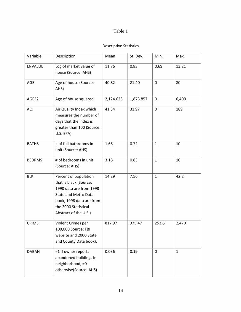
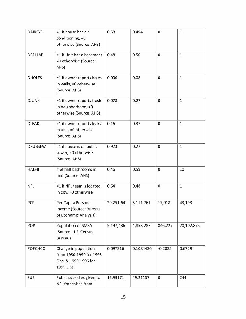
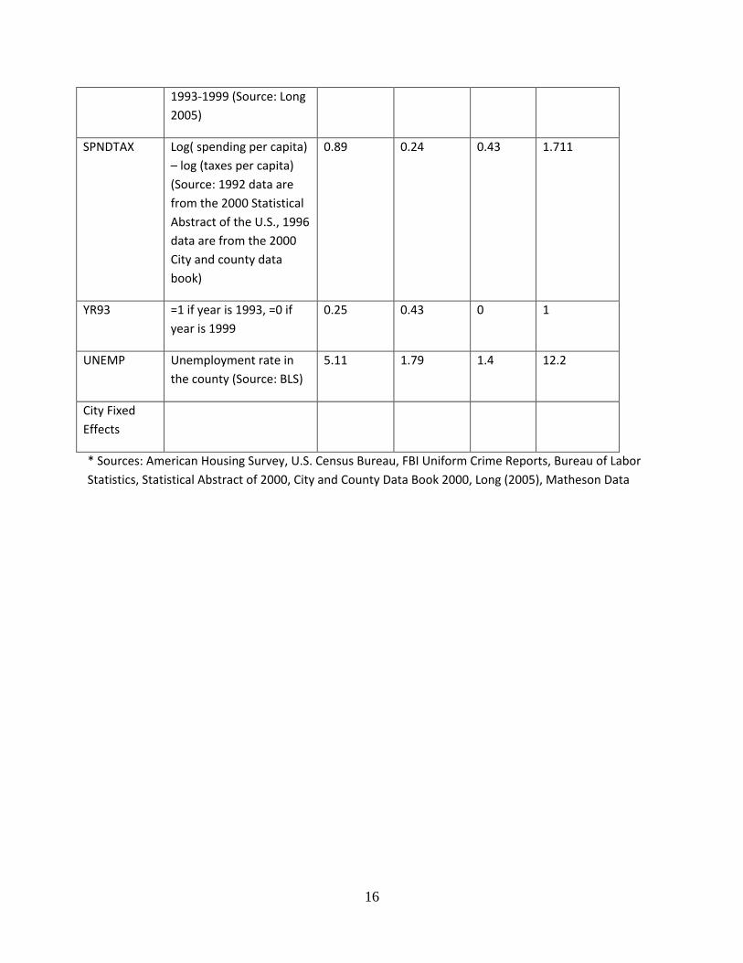
Table 1 provides a list of the variables included in our regressions along with descriptive

statistics. Because not all of Carlino and Coulson’s variables were well defined in their paper,

we approximated them as best we could. However, since the means for some of our variables

differ from theirs (e.g. population growth rate), it is likely that we are not including exactly the

same variables, but we should still be controlling for similar impacts. We have also added the

percent of the population in the city that is black, as well as whether the unit has a basement and

whether the owner reports leaks in the unit. We did not include whether the unit has a garage, is

detached, is in a low or high risk building, or includes monthly electricity costs in the rent. We

also do not include the resident-reported neighborhood crime and noise variables, nor whether

7

the unit is rent controlled or is subsidized. Thus we expect the same signs but not necessarily the

same coefficients.

Multicollinearity is a potential concern with this data set. Carlino and Coulson mention

multicollinearity between the NFL variable and air quality as a reason why some of their

coefficients are not statistically significant (page 42). In our data set the only variables with

correlations above 0.5 are Age and Age2, Yr93 and Unemp, Yr93 and PCPI, and Crime and

Unemp. Thus it seems unlikely that simple collinearity will cause problems in our estimated

regressions.

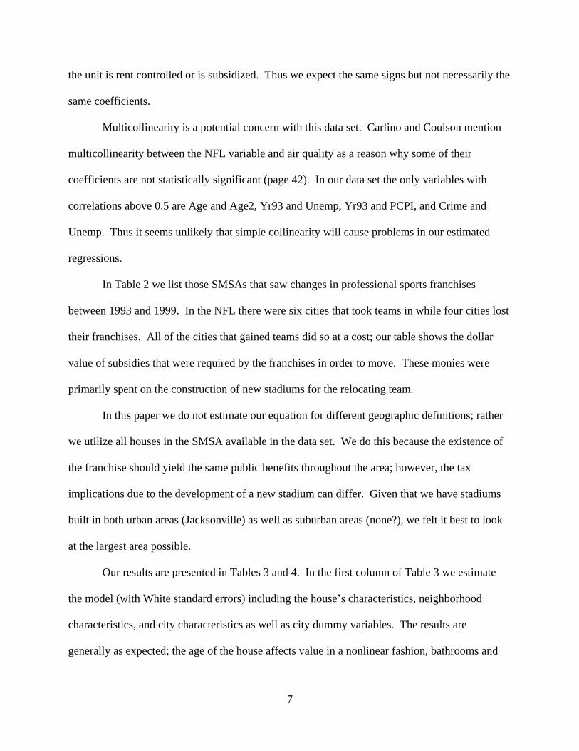
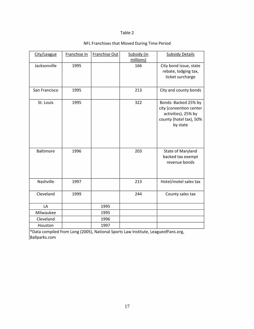
In Table 2 we list those SMSAs that saw changes in professional sports franchises

between 1993 and 1999. In the NFL there were six cities that took teams in while four cities lost

their franchises. All of the cities that gained teams did so at a cost; our table shows the dollar

value of subsidies that were required by the franchises in order to move. These monies were

primarily spent on the construction of new stadiums for the relocating team.

In this paper we do not estimate our equation for different geographic definitions; rather

we utilize all houses in the SMSA available in the data set. We do this because the existence of

the franchise should yield the same public benefits throughout the area; however, the tax

implications due to the development of a new stadium can differ. Given that we have stadiums

built in both urban areas (Jacksonville) as well as suburban areas (none?), we felt it best to look

at the largest area possible.

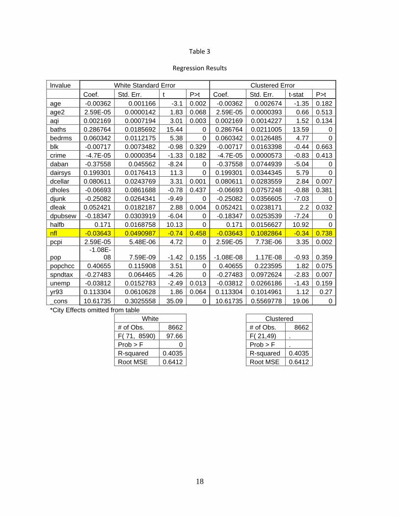
Our results are presented in Tables 3 and 4. In the first column of Table 3 we estimate

the model (with White standard errors) including the house’s characteristics, neighborhood

characteristics, and city characteristics as well as city dummy variables. The results are

generally as expected; the age of the house affects value in a nonlinear fashion, bathrooms and

8

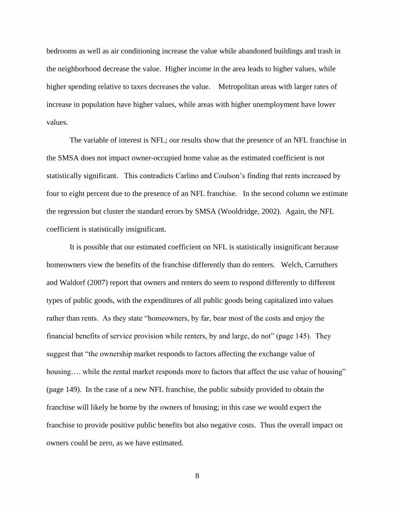
bedrooms as well as air conditioning increase the value while abandoned buildings and trash in

the neighborhood decrease the value. Higher income in the area leads to higher values, while

higher spending relative to taxes decreases the value. Metropolitan areas with larger rates of

increase in population have higher values, while areas with higher unemployment have lower

values.

The variable of interest is NFL; our results show that the presence of an NFL franchise in

the SMSA does not impact owner-occupied home value as the estimated coefficient is not

statistically significant. This contradicts Carlino and Coulson’s finding that rents increased by

four to eight percent due to the presence of an NFL franchise. In the second column we estimate

the regression but cluster the standard errors by SMSA (Wooldridge, 2002). Again, the NFL

coefficient is statistically insignificant.

It is possible that our estimated coefficient on NFL is statistically insignificant because

homeowners view the benefits of the franchise differently than do renters. Welch, Carruthers

and Waldorf (2007) report that owners and renters do seem to respond differently to different

types of public goods, with the expenditures of all public goods being capitalized into values

rather than rents. As they state “homeowners, by far, bear most of the costs and enjoy the

financial benefits of service provision while renters, by and large, do not” (page 145). They

suggest that “the ownership market responds to factors affecting the exchange value of

housing…. while the rental market responds more to factors that affect the use value of housing”

(page 149). In the case of a new NFL franchise, the public subsidy provided to obtain the

franchise will likely be borne by the owners of housing; in this case we would expect the

franchise to provide positive public benefits but also negative costs. Thus the overall impact on

owners could be zero, as we have estimated.

9

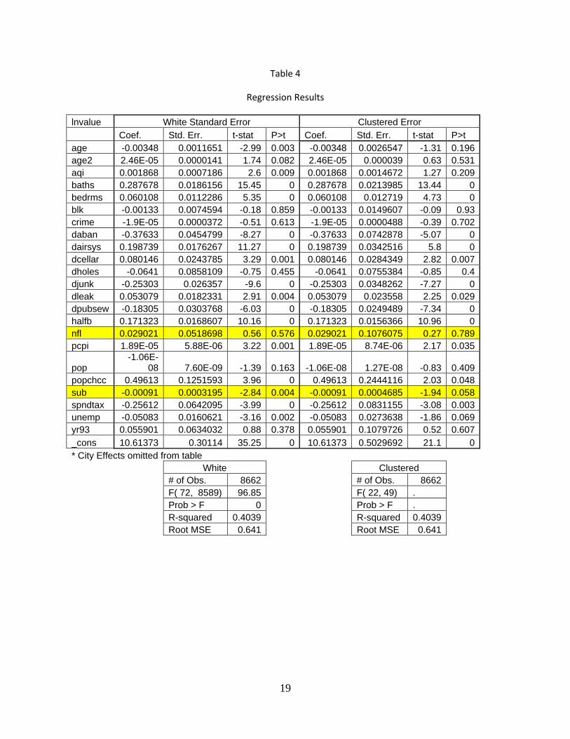
To test this hypothesis we include a variable that measures the amount of subsidy an

SMSA has paid to entice the franchise to their location. We can test whether these subsidies

result in increased local taxes, which are then capitalized into the house values. In Table 4

column 1 we report the results from the equation which also controls for the amount of the

subsidy that the team required (SUB). The NFL coefficient is still statistically insignificant;

however the estimated subsidy coefficient is negative and is statistically significant. This

indicates that those areas which have publicly funded the franchise do see a decrease in house

values of 0.091 percent. This is similar in magnitude to a one percent increase in the black

population in the city. In column 2 we estimate the same equation using the cluster technique for

the standard errors as before, and the results do not change.

Conclusions

In this paper we extend the work by Carlino and Coulson who suggest that sports

franchises are public goods that increase the quality of life in an area by examining the impact of

the franchises on housing values rather than rents. We find that the presence of an NFL

franchise does not lead to higher house values, all else held constant. We then test whether

those franchises that required public subsidies impact house values differently and find that

higher subsidies lead to lower house prices. This suggests that even if franchises do create

positive externalities, the capitalization of the required subsidies cause house prices to remain, on

average, unchanged.

Our results, when combined with those obtained by Carlino and Coulson, suggest that in

order to capture all costs and benefits of a sports franchise to an area, one must examine the

impact on both owners and renters. These two groups perceive the costs and benefits differently,

10

as others have found with other types of public goods. Indeed, the presence of an NFL team may

not be as beneficial to local residents as previous research has concluded.

11

References

Baade, R. 1996. Professional Sports as Catalysts for Metropolitan Economic Development.

Journal of Urban Affairs, 18(1): 1-17.

Baade, R. A. and A. R. Sanderson. 1997. The Employment Effect of Teams and Sports Facilities.

In Sports, Jobs & Taxes: The Economic Impact of Sports Teams and Stadiums, eds. R. G.

Noll and A. Zimbalist. Washington, DC.: Brookings Institution Press, , 92-118.

Baade, Robert A., Robert Baumann, and Victor A. Matheson. 2008. Selling the Game:

Estimating the Economic Impact of Professional Sports through Taxable Sales. Southern

Economic Journal, Vol. 74:3, 794-810.

Carlino, Gerald and N. Edward Coulson. 2004. Compensating differentials and the social

benefits of the NFL. Journal of Urban Economics, 56:1, 25-50.

Carlino, Gerald and N. Edward Coulson. 2006. Compensating differentials and the social

benefits of the NFL: Reply. Journal of Urban Economics, 60:1, 132-138.

Coates, D. and B. R. Humphreys. 1999. The Growth Effects of Sports Franchises, Stadia and

Arenas. Journal of Policy Analysis and Management, 18(4): 601-624.

Coates, D. and B. R. Humphreys. 2001. The Economic Consequences of Professional Sports

Strikes and Lockouts. Southern Economic Journal, 67(3): 737-747.

Coates, D. and B. R. Humphreys. 2003. The Effect of Professional Sports on Earnings and

Employment in the Services and Retail Sectors in U.S. Cities. Regional Science and

Urban Economics, 33:175-198.

Coates, D., B.R. Humphreys and A. Zimbalist. 2006. Compensating differentials and the social

benefits of the NFL: A Comment. Journal of Urban Economics, 60:1, 124 – 131.

12

Dehring, Carolyn A., Craig A. Depken and Michael R. Ward. 2007. A Direct Test of the Home

voter Hypothesis. North American Association of Sports Economists Working Paper

Series, Paper No. 07-19.

Freeman, A Myrick. 1993. The Measurement of Environmental and Resource Values; Theory

and Methods. Resources for the Future, Washington D.C.

Johnson, Bruce K., Peter A. Groothuis, John C. Whitehead. 2001. The Value of Public Goods

Generated by a Major League Sports Team: The CVM Approach. Journal of Sports

Economics, Vol. 2:1, 6-21.

Johnson, Bruce K., Peter A. Groothuis, John C. Whitehead. 2004. Public Funding of Professional

Sports Stadiums: Public Choice or Civic Pride? Eastern Economics Journal, Vol. 30:4,

515-526.

Johnson, Bruce K., Michael J. Mondello, and John C. Whitehead. 2006. Contingent Valuation of

Sports: Temporal Embedding and Ordering Effects Journal of Sports Economics, Vol.

7:3, 267-288.

Kiel, K.A. and J. E. Zabel. 1999. The Accuracy of Owner Provided House Values: The 1978-

1991 American Housing Survey Real Estate Economics 27(2):263-298.

Lavoie, M., and G. Rodriguez. 2005. The Economic Impact of Professional Teams on Monthly

Hotel Occupancy Rates of Canadian Cities: A Box-Jenkins Approach. Journal of Sports

Economics, 6(3): 314–24.

Lertwachara, K. and J. Cochran. 2007. An Event Study of the Economic Impact of Professional

Sport Franchises on Local U.S. Economies. Journal of Sports Economics, 8(3): 244-54.

Rosen, S. 1974. Hedonic prices and implicit markets: product differentiation in pure

competition. Journal of Political Economy, 82:34-55.

13

Taylor, Laura O. 2003. The Hedonic Method in A Primer on Nonmarket Valuation, edited by

Patricia A. Champ, Kevin J. Boyle and Thomas C. Brown. Kluwer Academic Publishers,

Dordrecht, Netherlands.

Welch, Robyn K., John I. Carruthers and Brigitte S. Waldorf. 2007. Public Service

Expenditures as Compensating Differentials in U.S. Metropolitan Areas: Housing Values

and Rents. Cityscape: A Journal of Policy Development and Research, 9(1): 131 – 156.

Wooldridge, Jeffrey M. 2002. Econometric Analysis of Cross Section and Panel Data. The

MIT Press, Cambridge, Massachusetts.

14

Table 1

Descriptive Statistics

Variable Description Mean St. Dev. Min. Max.

LNVALUE Log of market value of

house (Source: AHS)

11.76 0.83 0.69 13.21

AGE Age of house (Source:

AHS)

40.82 21.40 0 80

AGE^2 Age of house squared 2,124.623 1,873.857 0 6,400

AQI Air Quality Index which

measures the number of

days that the index is

greater than 100 (Source:

U.S. EPA)

41.34 31.97 0 189

BATHS # of full bathrooms in

unit (Source: AHS)

1.66 0.72 1 10

BEDRMS # of bedrooms in unit

(Source: AHS)

3.18 0.83 1 10

BLK Percent of population

that is black (Source:

1990 data are from 1998

State and Metro Data

book, 1998 data are from

the 2000 Statistical

Abstract of the U.S.)

14.29 7.56 1 42.2

CRIME Violent Crimes per

100,000 Source: FBI

website and 2000 State

and County Data book).

817.97 375.47 253.6 2,470

DABAN =1 if owner reports

abandoned buildings in

neighborhood, =0

otherwise(Source: AHS)

0.036 0.19 0 1

15

DAIRSYS =1 if house has air

conditioning, =0

otherwise (Source: AHS)

0.58 0.494 0 1

DCELLAR =1 if Unit has a basement

=0 otherwise (Source:

AHS)

0.48 0.50 0 1

DHOLES =1 if owner reports holes

in walls, =0 otherwise

(Source: AHS)

0.006 0.08 0 1

DJUNK =1 if owner reports trash

in neighborhood, =0

otherwise (Source: AHS)

0.078 0.27 0 1

DLEAK =1 if owner reports leaks

in unit, =0 otherwise

(Source: AHS)

0.16 0.37 0 1

DPUBSEW =1 if house is on public

sewer, =0 otherwise

(Source: AHS)

0.923 0.27 0 1

HALFB # of half bathrooms in

unit (Source: AHS)

0.46 0.59 0 10

NFL =1 if NFL team is located

in city, =0 otherwise

0.64 0.48 0 1

PCPI Per Capita Personal

Income (Source: Bureau

of Economic Analysis)

29,251.64 5,111.761 17,918 43,193

POP Population of SMSA

(Source: U.S. Census

Bureau)

5,197,436 4,853,287 846,227 20,102,875

POPCHCC Change in population

from 1980-1990 for 1993

Obs. & 1990-1996 for

1999 Obs.

0.097316 0.1084436 -0.2835 0.6729

SUB Public subsidies given to

NFL franchises from

12.99171 49.21137 0 244

16

1993-1999 (Source: Long

2005)

SPNDTAX Log( spending per capita)

– log (taxes per capita)

(Source: 1992 data are

from the 2000 Statistical

Abstract of the U.S., 1996

data are from the 2000

City and county data

book)

0.89 0.24 0.43 1.711

YR93 =1 if year is 1993, =0 if

year is 1999

0.25 0.43 0 1

UNEMP Unemployment rate in

the county (Source: BLS)

5.11 1.79 1.4 12.2

City Fixed

Effects

* Sources: American Housing Survey, U.S. Census Bureau, FBI Uniform Crime Reports, Bureau of Labor

Statistics, Statistical Abstract of 2000, City and County Data Book 2000, Long (2005), Matheson Data

17

Table 2

NFL Franchises that Moved During Time Period

City/League Franchise In Franchise Out Subsidy (in millions)

Subsidy Details

Jacksonville 1995 166 City bond issue, state rebate, lodging tax,

ticket surcharge

San Francisco 1995 213 City and county bonds

St. Louis 1995 322 Bonds: Backed 25% by city (convention center

activities), 25% by county (hotel tax), 50%

by state

Baltimore 1996 203 State of Maryland backed tax exempt

revenue bonds

Nashville 1997 213 Hotel/motel sales tax

Cleveland 1999 244 County sales tax

LA 1995

Milwaukee 1995

Cleveland 1996

Houston 1997

*Data compiled from Long (2005), National Sports Law Institute, LeagueofFans.org, Ballparks.com

18

Table 3

Regression Results

lnvalue White Standard Error Clustered Error

Coef. Std. Err. t P>t Coef. Std. Err. t-stat P>t

age -0.00362 0.001166 -3.1 0.002 -0.00362 0.002674 -1.35 0.182

age2 2.59E-05 0.0000142 1.83 0.068 2.59E-05 0.0000393 0.66 0.513

aqi 0.002169 0.0007194 3.01 0.003 0.002169 0.0014227 1.52 0.134

baths 0.286764 0.0185692 15.44 0 0.286764 0.0211005 13.59 0

bedrms 0.060342 0.0112175 5.38 0 0.060342 0.0126485 4.77 0

blk -0.00717 0.0073482 -0.98 0.329 -0.00717 0.0163398 -0.44 0.663

crime -4.7E-05 0.0000354 -1.33 0.182 -4.7E-05 0.0000573 -0.83 0.413

daban -0.37558 0.045562 -8.24 0 -0.37558 0.0744939 -5.04 0

dairsys 0.199301 0.0176413 11.3 0 0.199301 0.0344345 5.79 0

dcellar 0.080611 0.0243769 3.31 0.001 0.080611 0.0283559 2.84 0.007

dholes -0.06693 0.0861688 -0.78 0.437 -0.06693 0.0757248 -0.88 0.381

djunk -0.25082 0.0264341 -9.49 0 -0.25082 0.0356605 -7.03 0

dleak 0.052421 0.0182187 2.88 0.004 0.052421 0.0238171 2.2 0.032

dpubsew -0.18347 0.0303919 -6.04 0 -0.18347 0.0253539 -7.24 0

halfb 0.171 0.0168758 10.13 0 0.171 0.0156627 10.92 0

nfl -0.03643 0.0490987 -0.74 0.458 -0.03643 0.1082864 -0.34 0.738

pcpi 2.59E-05 5.48E-06 4.72 0 2.59E-05 7.73E-06 3.35 0.002

pop -1.08E-

08 7.59E-09 -1.42 0.155 -1.08E-08 1.17E-08 -0.93 0.359

popchcc 0.40655 0.115908 3.51 0 0.40655 0.223595 1.82 0.075

spndtax -0.27483 0.064465 -4.26 0 -0.27483 0.0972624 -2.83 0.007

unemp -0.03812 0.0152783 -2.49 0.013 -0.03812 0.0266186 -1.43 0.159

yr93 0.113304 0.0610628 1.86 0.064 0.113304 0.1014961 1.12 0.27

_cons 10.61735 0.3025558 35.09 0 10.61735 0.5569778 19.06 0

*City Effects omitted from table

White Clustered

# of Obs. 8662 # of Obs. 8662

F( 71, 8590) 97.66 F( 21,49) .

Prob > F 0 Prob > F .

R-squared 0.4035 R-squared 0.4035

Root MSE 0.6412 Root MSE 0.6412

19

Table 4

Regression Results

lnvalue White Standard Error Clustered Error

Coef. Std. Err. t-stat P>t Coef. Std. Err. t-stat P>t

age -0.00348 0.0011651 -2.99 0.003 -0.00348 0.0026547 -1.31 0.196

age2 2.46E-05 0.0000141 1.74 0.082 2.46E-05 0.000039 0.63 0.531

aqi 0.001868 0.0007186 2.6 0.009 0.001868 0.0014672 1.27 0.209

baths 0.287678 0.0186156 15.45 0 0.287678 0.0213985 13.44 0

bedrms 0.060108 0.0112286 5.35 0 0.060108 0.012719 4.73 0

blk -0.00133 0.0074594 -0.18 0.859 -0.00133 0.0149607 -0.09 0.93

crime -1.9E-05 0.0000372 -0.51 0.613 -1.9E-05 0.0000488 -0.39 0.702

daban -0.37633 0.0454799 -8.27 0 -0.37633 0.0742878 -5.07 0

dairsys 0.198739 0.0176267 11.27 0 0.198739 0.0342516 5.8 0

dcellar 0.080146 0.0243785 3.29 0.001 0.080146 0.0284349 2.82 0.007

dholes -0.0641 0.0858109 -0.75 0.455 -0.0641 0.0755384 -0.85 0.4

djunk -0.25303 0.026357 -9.6 0 -0.25303 0.0348262 -7.27 0

dleak 0.053079 0.0182331 2.91 0.004 0.053079 0.023558 2.25 0.029

dpubsew -0.18305 0.0303768 -6.03 0 -0.18305 0.0249489 -7.34 0

halfb 0.171323 0.0168607 10.16 0 0.171323 0.0156366 10.96 0

nfl 0.029021 0.0518698 0.56 0.576 0.029021 0.1076075 0.27 0.789

pcpi 1.89E-05 5.88E-06 3.22 0.001 1.89E-05 8.74E-06 2.17 0.035

pop -1.06E-

08 7.60E-09 -1.39 0.163 -1.06E-08 1.27E-08 -0.83 0.409

popchcc 0.49613 0.1251593 3.96 0 0.49613 0.2444116 2.03 0.048

sub -0.00091 0.0003195 -2.84 0.004 -0.00091 0.0004685 -1.94 0.058

spndtax -0.25612 0.0642095 -3.99 0 -0.25612 0.0831155 -3.08 0.003

unemp -0.05083 0.0160621 -3.16 0.002 -0.05083 0.0273638 -1.86 0.069

yr93 0.055901 0.0634032 0.88 0.378 0.055901 0.1079726 0.52 0.607

_cons 10.61373 0.30114 35.25 0 10.61373 0.5029692 21.1 0

* City Effects omitted from table

White Clustered

# of Obs. 8662 # of Obs. 8662

F( 72, 8589) 96.85 F( 22, 49) .

Prob > F 0 Prob > F .

R-squared 0.4039 R-squared 0.4039

Root MSE 0.641 Root MSE 0.641