estimating the technical efficiency, shadow price and ... paper... · marginal abatement cost of...
TRANSCRIPT

1
Estimating the technical efficiency, shadow price and substitutability
of SO2 emissions in Chinese second industry: A panel data analysis
with a parametric methodology
Huiming XIE Manhong SHEN Chu WEI
Abstract Due to the severe air pollution of the smog and acid rain, further actions to reduce the SO2
emission is urgent for the current China. This paper investigates the four important aspects of SO2
emission reductions in the second industry based on a province-year panel data from 1998 to 2011
via a parametric methodology: technical efficiency, shadow price, potential reduction and
Morishima elasticity. The results show that the disparities of the above four aspects are significant
among the provinces and the three regions. The technical efficiency is improved in a non-linear
form over times. The potential reductions of SO2 in the east and middle converge to some extent
during the whole period, while the west becomes dominated in the SO2 emission reductions. The
shadow prices keep the similar increasing path in the west and the middle while the price in the
east increased much more and become the most expensive in 2011 at the beginning of the 12th
Five-Year Plan. The substitution elasticity highlights the difficulties of reducing the SO2
emissions.
Keywords: SO2 emission; Shadow price; Substitutability; Parametric Estimation; China
Huiming XIE Manhong SHEN Chu WEI
Corresponding Author:
School of School of School of Economics,
Economics and Management, Economics and Management, Renmin University of China,
Zhejiang Sci-tech University, Zhejiang Sci-tech University, Beijing 100872, China
Hangzhou 310018, China Hangzhou 310018, China Tel:+0086 18811553981
E-mail: E-mail: E-mail:

2
1. Introduction
As a result of urbanization, industrialization, China is now the world’s largest energy
consumer and air pollution has been a big environmental problem. One outstanding phenomena of
Chinese air pollution is smog, which is widely reported both home and abroad in 2013. The smog
once darkened the skies over China for the past decades (NASA, 2006), now persists across
northern China and touches the Yangtze River (CMA, 2013). Atmospheric sulfur dioxide (SO2)
emission is the major contributor to PM2.5 and is considered as the main factor of the smog.
Meanwhile, sulfate can result in serious health impact (Pathak et al., 2009), contribute to acid
deposition and billions of economic losses (Hao et al., 2007; Wei et al. 2014). As a result, in order
to improve the air quality, China’s central, provincial and local governments have implemented a
suite of evolving polices and programs to reduce the SO2 emissions.
China issued the first law on the prevention and control of air pollution in 1987 and revised
twice in 1995 and 2000 with more detailed articles on SO2. The revisions in 2003 and 2011
focused on the main contributor of SO2: thermal power plants, and several emission concentration
limits were put forward. Except for the laws on the prevention and control of atmospheric
pollution, Five-Year Plan (FYP) has become more and more important government documents in
China and plays more important role in SO2 reductions. In the 9th FYP, the central government
established SO2 emission targets for key sectors and regions, then in the 10th FYP the central
government established national objectives to control SO2 emissions. However, the government
failed to reduce SO2 emissions an average of by 10% below 2001 (NBS, 2004), and the second
attempt in the 11th FYP (2006-2010) was successful, total SO2 emissions declined by more than
14% by the end of 2010 (Wen, 2011). The factors contributed to the achievement of the 11th FYP
include instrument choice, political accountability, emission verification, political support,
streamlined targets and political and financial incentives (Schreifels et al., 2012). Based on all the
experiences and achievements of 11th FYP, the target of SO2 emission in the 12th FYP is set at 8%.
Overall China is actively engaging in air quality protection by law and four FYPs have also
focused on the SO2 for more than10 years. We may be glad to hear about that we achieve a lot and

3
experienced a lot, but the smog becomes more and more heavy and the acid rain pollution is still
serious (MEP, 2012). As a result, what we need to pay more attention to is controlling the
ecological functions for different ecological system or regions and further actions to reduce the
SO2 emissions are still urgently needed to be implemented by both the central, provincial and local
government (Wang et al., 2012; Wang and Hao, 2012). Economic effective way to reduce SO2
emission is essential. Meanwhile, why the abatement target of SO2 drops to 8% in 12th? Does it
mean that the government encountered some obstacles in the process of SO2 emission reductions?
Is it because of the poor policy implementation? Or low technical efficiency? Or no more potential
reductions of SO2? In order to answer these questions, we need to estimate the technical efficiency,
marginal abatement cost of SO2 or shadow price, potential reduction etc..
The reminder of this paper is arranged as follows: section 2 reviews the previous literatures;
section 3 put forward a theoretical model of directional distance function and section 4 gives out
an empirical specification of quadratic form. Section 5 describes the data and section 6 reports the
estimation results. Several conclusions are summarized in the last section.
2. Literature review
Shadow price study started from the cost-benefit analysis. Gollop and Roberts (1985)
estimated the shadow price of SO2 based on 56 electricity plants of US in the period 1973-1979 by
minimizing the costs of generating electricity. The price of SO2 is $0.195 per bond in 1979 price.
After Färe et al. (1993) adopted distance function to estimated the shadow price of BOD, SOX et
al., Coggins and Swinton (1996) used distance function in translog form to estimate the shadow
price of SO2 based the analysis of 14 electricity plants in Wisconsin between 1990 and 1992. The
average estimated price is $292.7 per ton in 1992 price and the technical efficiency is 0.946. While
in Florida, the estimated price is $157.1 per ton in 1996 price using the same model and
methodology based on coal-burning electricity plants from 1990-1998 (Swinton, 1998). Or the
price might be $395.3 per ton in 1980, $1871.7 per ton in 1985, $556.8 per ton in 1990 and $486.7
per ton in 1995 based on distance function with translog form(Atkinson and Dorfman, 2005).
Recent development in shadow price of non-market pollutants is to use directional output
distance function, which allows a simultaneous expansion of good outputs and contraction of bad

4
outputs along the given direction (Chamber et al., 1998; Chung et al., 1997). The directional
distance function is newly considered more appropriate for measuring performance in the presence
of bad output under regulation (Färe et al., 1993; Färe et al., 2005). There are two strategies to
estimate the directional output distance function and shadow price. One is non-parametric
approach, namely data envelopment analysis (DEA), and the other is parametric estimation.
As regard non-parametric estimation, Boyd et al. (1996) used DEA to estimate the directional
distance function and the average value is 0.933, which refers to the technical efficiency, and
shadow price of SO2 was also estimated, which is about $1703 per ton in 1973 price. Lee et al.
(2002) used a nonparametric directional distance function approach to estimate the shadow prices
of pollutants like sulfur oxides and nitrogen oxides and total suspended particulates (TSP). The
estimated price of sulfur oxides is $-3107 per ton, which is 10% lower than those calculated under
the assumption of full efficiency. Such other nonparametric methods as Convex Nonparametric
Least Squares (CNLS) (Kuosmanen, 2008) and Stochastic Nonparametric Envelopment of Data
(StoNED) (Kuosmanen and Kortelainen, 2012) were developed and used to estimate the shadow
price of CO2 (Mekaroonreung and Johnson, 2012).
However, the distance function estimated via nonparametric method is not differentiable, thus
it is less well-suited to the estimation of shadow price and elasticity of substitutions and can not
deal with the outliers (Färe et al., 2005; Vardanyan and Noh, 2006). Many researchers use
parametric estimation to estimate the shadow price of SO2 (Salnykov and Zelenyuk, 2004; Färe et
al., 2005). The parametric estimation pre-assumes a specific functional form for the distance
function and then estimates the parameters of the distance function. Once the parameters are
estimated, it is easy to calculate the directional distance function, the shadow price and the
substitution elasticity. In empirical study, quadratic function form is usually specified in estimating
the directional output distance function (Du et al., 2013).
As regard the research on the SO2 emission reductions in China, to our best knowledge there
are few papers investigated the marginal abatement cost of SO2 emissions. Ke et al. (2008) use
output distance function via parametric linear programming to estimate the shadow price and
distance function for 30 provinces in China during the 1996-2003 period. They found that the east

5
was the most efficient and the central is the most inefficient, while shadow price in the west was
highest and it was lowest in the central. The average efficiency for all the 30 provinces during the
period is 0.731-0.761 and the shadow price is 50.9-54 million Yuan per ton. Kaneko et al. (2010)
focused on the plant level to estimate the shadow price of SO2 using the directional distance
function via a nonparametric approach. The results show that the marginal abatement cost has
significantly decline in recent years due to the application of desulfurization technology in China
and certain budget scale would have significant outcomes on SO2 reductions. Kanada et al. (2013)
analyzed 5 mega-cities in China and clarified that reduction potential and cost-effectiveness were
closely linked to regional disparity, Beijing and Hong Kong showed lower reduction potential and
higher marginal reduction cost while Chongqing showed the largest reduction potential and the
lowest marginal reduction cost.
However, such researches on the issues of Chinese SO2 emission reductions reported the
technical efficiency and the shadow price but no potential reductions of SO2, or use GAINS-China
model to analyze the potential reductions and its reduction cost. In terms of the model and
methodology, both the distance function and directional distance function have been used. But the
parametric methodology is used when distance function is adopted; or the nonparametric
methodology is used when the directional distance function is adopted. So this paper combines the
directional distance function and parametric methodology together for estimating the shadow price
and technical efficiency of the 30 provinces in China during 1998-2011, which contains the 4
FYPs (9th, 10th, 11th and 12th). The second industry has the highest emissions of SO2 emissions per
unit of output value compared with the primary and tertiary industries in China (Yuan et al., 2013).
A longer time period is more meaningful for the governments to testing the SO2 emission
reduction policies and programs. Further more, we also conduct the estimations of potential
reductions of SO2 during the 4 FYPs and the Morishima elasticity indicating the cost-effectiveness
for abatement, which are all helpful for debate on the optimal abatement policies in China.
3. Model
In this section, we firstly define the parameterized directional output distance function and
calculate the potential reduction of SO2 in quadratic form to be obtainable by assuming a technical

6
efficiency of 100%. The typical Morishima elasticity of substitution is then calculated for the
measurement of how the good-bad shadow price ratio changes as the relative pollution intensity
changes (Färe et al., 2005), an the shadow price of SO2 is derived by assessing the marginal
abatement of SO2 emissions of each province.
3.1 The directional output distance function
Let us consider a productive process that produces a vector of outputs ( ) 2, +ÂÎby using a
vector of inputs 3+ÂÎx . The vector of outputs contains the desirable output ( y ) and undesirable
output (b ), SO2 emissions, as a byproduct generated by burning fossil fuels; the vector of inputs
can be divided into two kinds: non-energy inputs including capital ( k ) and labor ( l ), and energy
input ( e ) which is calculated by the standard coal equivalent of coal, oil and gas, including raw
coal, clean coal, briquettes, coke, coke oven gas, crude oil, gasoline, kerosene, etc. We then define
production technology as the following output set
( ) ( ){ xbyxP :,= can produce ( )}by, (1)
The above output set needs to satisfies the standard assumptions of compact and freely
disposable in inputs, more additional assumptions are imposed: (1) Joint production: if
( ) ( )xPby Î, and 0=b then 0=y . It means that no desirable output can be simultaneously
produced without undesirable output; (2) Weak disposability: if ( ) ( )xPby Î, and 10 ££q ,
then ( ) ( )xPby Îqq , . It indicates that any reduction of undesirable output carries a cost in the
feasible proportional reduction of both desirable and undesirable outputs; (3) Free disposability: if
( ) ( )xPby Î, and yy £¢ , then ( ) ( )xPby ΢, . It implies that no extra cost will be incurred in the
process of disposing some of desirable outputs.
In line with the above assumptions, the directional output distance function is defined as
( ) ( ) ( ){ }xPgbgyggbyxD bybyo Î-+=- bbb ,:max,;,,r
(2)
Where ( ) 11, ++ ´ÂÎ= by ggg indicates the direction of output vector, which describes the
simultaneous maximum expansion of desirable outputs and contraction of undesirable outputs.

7
Fig.1 provides the intuitional image of such a function of formula (1). ( )xP illustrates the
production technology and ( ) 0, >= by ggg is the direction vector which implies the combined
outputs including both the desirable output y and undesirable outputb reaches the boundary of
( )xP in g ’s direction. Taking an observation ( )byA , for example, it lies within the boundary and
can increase y and reduceb simultaneously to hit the boundary at point ( )by gbgyB ** , bb -+ ,
where ( )byo ggbyxD -= ,;,,*r
b . The value ofb describes the inefficiency of production. A zero
value means that this producer located on the frontier and performed efficiently in g ’s direction
while a positive value reflects the existence of inefficiency. The higher the value ofb , the lower
efficiency is the output vector.
Figure 1: Directional Output Distance Function
In accordance with the inherited properties of the directional output distance function (Färe et
al., 2005), the following six properties are needed to be satisfied
a) ( ) 0,;,, ³- byo ggbyxDr
if and only if ( )by, is an element of ( )xP
b) ( ) ( )byobyo ggbyxDggbyxD -³-¢ ,;,,,;,,rr
for ( ) ( ) ( )xPbyby 룢 ,,
c) ( ) ( )byobyo ggbyxDggbyxD -³-¢ ,;,,,;,,rr
for ( ) ( ) ( )xPbyby γ¢ ,,
d) ( ) 0,;,, ³- byo ggbyxD qqr
for ( ) ( )xPby Î, and 10 ££q

8
e) ( ) 0,;,, ³- byo ggbyxDr
is concave in ( ) ( )xPby Î,
f) ( ) ( ) aaa --=--+ byobybyo ggbyxDgggbgyxD ,;,,,;,,rr
Non-negative property is shown in the first property and the second property indicates
that b decreases monotonically as the desirable outputs increase. Otherwise, the efficiency will be
lower when there are more undesirable outputs, which is depicted in the third property. The forth
property corresponds to weak disposability and the sign of the output elasticity of substitution is
determined in the fifth. The last property shows that the directional distance function needs to
satisfy the translation property. If desirable output is expanded by yga and undesirable output is
contracted by bga simultaneously, the inefficiency of a decision-making unit (DMU) will be
reduced by a scalara .
3.2 The showdown price of SO2
Following Färe et al. (2006), the revenue function can be derived by solving the problem of
revenue-maximization subject to the directional distance function constraint
( ) ( ){ }0;,,:max,, ³-= gbyxDqbpyqpxR o
r (3)
Where 1+ÂÎp is the vector of prices of desirable output y and 1
+ÂÎq is the vector of prices of
undesirable outputb .
Given a feasible directional vector ( )by ggg ,= showing a DMU moves the production
in g ’s direction, then we will have
( ) ( ) ( ) ( ) boyo ggbyxDqggbyxDpqbpyqpxR ;,,;,,,,rr
++-³ (4)
Where the left side is the maximum feasible revenue and the right side represents the observed
revenue plus technical efficiency gains containing two components, the gain due to an increase in
desirable outputs and decrease in undesirable outputs. Rearranging the formula (4), we have
( ) ( ) ( ) ( ) ( )ïþ
ïýü
ïî
ïíì
+--
=+
--£
byqp
byo qgpg
qbpyqpxRqgpg
qbpyqpxRgbyxD
,,min
,,;,,
,
r (5)
Both directional distance function and revenue function are differentiable is assumed, and the
first-order conditions of formula (5) are formula (6) and (7).

9
( )by
oy qgpgp
gbyxD+-
=Ñ ;,,r
(6)
( )by
ob qgpgq
gbyxD+-
=Ñ ;,,r
(7)
As a result, given the market price of the desirable output, the shadow price of the SO2 can be
calculated as formula (8). In order to completely characterize the technology, ( )1,1 -=g is
imposed under g-disposability.
( )( ) ú
û
ùêë
é¶-¶¶-
-=ybyxDbbyxD
pqo
o
1,1;,,1,1;,,r
r (8)
As is shown in Fig.1, the ratio of the shadow price ( pq- ) for an observation with
coordinates ( )by, is the tangent evaluation of the boundary of ( )xP . In terms of one desirable
output and one undesirable output, the formula (8) measures the shadow price of the undesirable
output when the good and bad outputs are traded off on the frontier.
3.3 The Morishima elasticity of substitution
Morishima elasticity of substitution measures how the desirable-undesirable shadow price
ratio changes as the relative pollution intensity changes (ratio of undesirables to desirables)..
Following Färe et al. (2005), the Morishima elasticity is defined as:
( )( )by
pqMby ln
ln¶¶
= (9)
Based on formula (8), byM can be specified as
( )( )
( )( ) ú
û
ùêë
鶶¶¶
-¶¶¶¶
=ygbyxD
yygbyxDbgbyxD
ybgbyxDyM
o
o
o
oby ;,,
;,,;,,;,, 22
* rr
rr
(10)
Where ( )1,1;,,* -+= byxDyy o
r. The sign of byM is negative under certain conditions and its
larger value reflects lower substitutability. That is to say when byM is more negative it will be
more costly for the DMU to reduce the undesirable output due to the higher substitutability.

10
4. Empirical Specification
Computation of inefficiencyb in formula (2), shadow price q in formula (8) and Morishima
elasticity byM in formula (10), the quadratic form to parameterize the directional output distance
function is selected based on the previous works done by Chambers et al. (1998), Färe et al.
(2005) , Murty et al. (2007) and Wei et al. (2013).
( )
( ) ( ) å å
ååå
= =
= =¢¢¢
=
+++++
++++=-
3
1
3
1
2
2
2
2
3
1
3
111
3
1
21
21
21
1,1;,,
n n
tk
tk
tk
tnkn
tk
tnkn
tk
tk
n n
tkn
tnknn
tk
tk
n
tnkn
tk
tk
tko
byyxbxby
xxbyxbyxD
mdhgb
agbaar
(11)
Where there are Kk L,1= provinces producing in Tt L,1= years. Meanwhile, a set of
provincial dummy and timing dummy in the intercept term is added in formula (12) as Färe et al.
(2006) have done:
åå-
=
-
=
++=1
1
1
10
T
ttt
K
kkk TSaa tl (12)
where kl and tt are the coefficients of the provincial and timing dummies respectively. The
province dummy variable 1=¢kS if kk =¢ , and 0 otherwise; similar setting is for timing dummy.
To estimate the parameters in formula (11) and (12), we employ the linear programming technique
originally adopted by Aigner and Chu (1968), which has the advantage to impose parametric
restrictions on quadratic functions.
min ( )( )åå= =
--T
t
K
k
tk
tk
tko byxD
1 1
01,1;,,r
s.t. a) ( ) 01,1;,, ³-tk
tk
tko byxD
r, Kk L,1= ; Tt L,1=
b) ( ) 01,1;0,, <-tk
tko yxD
r, Kk L,1= ; Tt L,1=
c)( )
01,1;,,³
¶-
bbyxD t
ktk
tko
r, Kk L,1= ; Tt L,1=
d)( )
01,1;,,£
¶-
ybyxD t
ktk
tko
r, Kk L,1= ; Tt L,1=

11
e)( )
01,1;,,³
¶-
n
tk
tko
xbyxD
r, 3,2,1=n ; Kk L,1= ; Tt L,1=
f) 111 -=- gb , mgb == 22 , nn hd = , 3,2,1=n
g) nnnn ,, ¢¢ = aa , 3,2,1, =¢nn
The objective function is to narrow the gap between the boundary and individual
observations, subject to the following constraints: all observations are feasible, which implies that
all each observation is located on or below the boundary; null-jointness property which means that
the output bundle ( )0,y is not technically feasible for 0>y (Marklund and Samakovlis,
2007); Monotonicity assumption in bad and good outputs; positive monotonicity constraints in
inputs for the mean level; translation property and symmetry restriction.
Once the parameters of the directional output distance function are all estimated, the shadow
price of the bad output and Morishima substitution elasticity for each province in each year could
be calculated. The equation (8) and (10) could be empirically rewritten as (13) and (14):
úúúú
û
ù
êêêê
ë
é
+++
+++-=
å
å
=
=3
121
3
121
nnn
nnn
bxy
yxbpq
mdbb
mhgg (13)
úúúú
û
ù
êêêê
ë
é
+++-
+++=
åå==
3
121
23
121
nnn
nnn
by
bxyyxbyM
mdbb
b
mhgg
m (14)
5. Data and Descriptive Statistics
The directional output distance function is estimated using a province-by-year panel dataset
covering 30 provinces of China in the period 1998-2011. The desirable output ( y ) and capital
input ( 1x ) are measured, respectively, as the gross industrial product value (GIOV) and net value
of fixed assets deflated to the 2005 price. The undesirable output (b ) is considered and measured
as volume of SO2 emission. Labor input ( 2x ) is the annual average number of employees. Those
data are collected from the China Statistical Yearbook. Energy input ( 3x ) include all the available

12
types in the China Energy Statistical Yearbook and are measured as tons of coal equivalent (TCE)
on the basis of the conversion factors ( cf ). The energy input is calculated as follows:
Energy input = jj
j cfec ´å=
20
1
Where ec refers to the energy consumption and j =20 types of energy are calculated. Table 1
shows the conversion factors for different types of fuel. The statistics for data used are
summarized in Table 2.
Table 1: Conversion factors from physical units to coal equivalent (kgce/kg)
Energy cf Energy cf Energy cf Energy cf
Raw coal 0.7143 Other gas 0.1786 Fuel oil 1.4286 Electricity 0.1229
Clean coal 0.900 Crude oil 1.4286 LPG 1.7143 Other washed coal 0.2857
Briquettes 0.6594 Gasoline 1.4714 Refinery gas 1.5714 Other coking product 1.1429
Coke 0.9714 Kerosene 1.4714 Natural gas 1.3300 Other petrol product 1.4143
Coke oven gas 0.5714 Diesel oil 1.4571 Heat 0.0341 Other energy 1
Source: China Energy Statistical Yearbook, Department of Energy Statistics, National Bureau of Statistics, China.
Table 2: Descriptive Statistics (T=14, K=30, sample size=420)
Outputs and inputs Variable Unit Mean Std. Dev. Min Max
y :GIOV 108 Yuan 9651 14427 182 91124 Output
b :SO2 104 Ton 60.77 39.02 1.9 176
1x :Capital 108 Yuan 3446 3355 197 18778
Non-Energy Input
2x :Labor 104 Person 235 253 9.62 1568
Energy Input 3x :TCE 104 Ton 2384 1899 52.67 10876
6. Empirical Results
To avoid the convergence problem, all the variables are normalized at the mean (Färe et al.,
2005), which means that ( ) ( )1,1,1,, =byx for a hypothetical province using mean inputs to
produce mean outputs. Table 3 presents the parameter estimates for the directional distance
function equation (11), which are obtained by solving the linear programming using GAMS. In

13
order to get the degree of technical efficiency, we insert those parameters back into equation (11),
and then the shadow price of bad output and Morishima elasticity of substitution could also be
obtained once the parameters are all given.
Table 3: Parameter Estimates of Directional Distance Function
Parameters Estimates Parameters Estimates Parameters Estimates Parameters Estimates
0a 0.107 11a 0.219 31a -0.123 2h -0.133
1a 0.391 12a -0.096 32a 0.445 3h 0.026
2a 0.296 13a -0.123 33a -0.178 1d -0.041
3a -0.109 21a -0.096 2b 0.114 2d -0.133
1b -0.800 22a 0.046 2g 0.114 3d 0.026
1g 0.200 23a 0.445 1h -0.041 m 0.114
6.1 Technical Inefficiency
As the directional output distance function gives the maximum unit expansion of the
desirable output and contraction of the undesirable output, it is severed as the measurement of
technical inefficiency. Statistically, the production is fully efficient with a zero directional distance
function, and higher score of the directional output function mean lower technical efficiency.
Figure 2 depicts the kernel densities of the estimates of provincial directional output distance
functions for selected years, 1998, 2002, 2005 and 2011. More estimated results are reported in
Table 1A appended. It is shown that, in Figure 2, the kernel density curve moves leftward firstly
and then moves rightward back to the original in 2011. The peaks of the curves also become
higher for the several starting years of the sample and then move downward. As a result, the
technical efficiency does not change in the same direction during the period 1998 to 2011, which
could be divided into two periods: upward period and downward period.

14
01
23
45
Ker
nel D
ensi
ty
0 .2 .4 .6 .8Directional Output Distance Function
1998 20022005 2011
Figure 2: Kernel Density of Directional Output Distance Function
In order to probe into the two periodic route of technical efficiency of the 30 provinces in
China, three Chinese typical regions are clarified: the east, the middle and the west. East region
includes Beijing, Tianjin, Hebei, Liaoning, Shanghai, Jiangsu, Zhejiang, Fujian, Shandong,
Guangdong and Hainan, Middle region includes Shanxi, Jilin, Heilongjiang, Anhui, Jiangxi,
Henan, Hubei and Hunan. West region includes Inner Mongolia, Guangxi, Sichuan, Chongqing,
Guizhou, Yunnan, Shaanxi, Gansu, Qinghai, Ningxia and Xinjiang. Figure 3 repots the technical
inefficiency for the east, the middle, the west and the whole country as the time elapses. Detailed
provincial results of the technical inefficiency are reported in table 1A. From Figure 3, we can
observe that the directional distance function become lower for almost years in the east, indicating
that the technical efficiency of SO2 reductions is improved a lot during the whole period. In the
middle region, the technical efficiency experienced a dispersed U-shape in the whole period,
which means the technical efficiency returned to the level of 1998 in 2009 and became lower in
2010 and 2011. As regard the west, the technical inefficiency is almost increasing rapidly during
the whole period. Though the technical efficiency of the different regions are significantly
different, it decreased firstly and then increased in terms of the whole country, shaping a dispersed

15
U, the results are in line with the results of the kernel density analysis and 2008 is considered as
the year at the turning point.
0.00
0.05
0.10
0.15
0.20
0.25
0.30
0.35
0.40
0.45
1998 1999 2000 2001 2002 2003 2004 2005 2006 2007 2008 2009 2010 2011
Dire
ctio
nal O
utpu
t Dis
tanc
e Fu
nctio
n
East Middle West China
Figure 3: Average Technical Inefficiency by Region
6.2 Potential Reduction of SO2 emissions
Assuming that the use of energy could be reduced by the technical inefficiency along with
other inputs, we can calculate the maximum SO2 emission that could be reduced by individual
province by achieving 100% technical efficiency. The formula is:
ktktktktktktktktkt bbbbbbb bb =--=-=D )(*
Where t is referred to the year and k donates the province. *ktb is the minimum attainable level of
emissions for province k in year t. However, due to the heterogeneity of the provinces, it is
difficult to compare the potential reduction of each province based on its size or output. To that
end, we take the average potential reduction of SO2 emissions of each region by dividing the
average potential reduction of the whole country, which accounts for the percentage of average
potential reductions of SO2 by the region.

16
0
0.5
1
1.5
2
2.5
1998 1999 2000 2001 2002 2003 2004 2005 2006 2007 2008 2009 2010 2011
Perc
enta
ge(1
00%
)
East Middle West
Figure 4 Percentage of Average Potential Reduction by Region
Figure 4 posts the percentage of average potential reduction of the three regions. From the
Figure 4, we observe that the percentage of potential reduction of SO2 in the east become lower
and lower, and is less than the west eventually in 2009 and the middle in 2010. As regard the west,
the percentage of potential reduction of SO2 increased a lot during the period 1998-2010; while in
the middle, the percentage of potential reduction of SO2 does not change a lot. It could be
concluded that the market structure of the potential reduction of SO2 is transferring from the east
dominated to the west dominated while the east and the middle market are converging at last in
2011.
6.3 Shadow Prices of SO2 Emissions
The estimated shadow prices of SO2 or marginal SO2 abatement costs from equation (13) are
presented in Table 2A. The average marginal abatement cost of SO2 in China from 1998 to 2011
increased from 0.42 to 1.5 million Yuan per ton. Specifically, the marginal abatement for the 30
provinces in the period 1998-2011 ranged from 0.03 million Yuan which occurred in Shandong in
1999 to 1.167 million Yuan in Shandong in 2011.

17
0.0
1.0
2.0
3.0
4K
erne
l Den
sity
0 50 100 150Shadow Price, 10000 Yuan
1998 20022005 2011
Figure 5: Kernel Density of Shadow Price
The kernel density curves of the shadow prices for selected year are posted in Figure 5. From
this figure, we observe that the kernel density curves move rightward over time, and the dispersion
rage of points become wider. It means that the mean value and the variance of the shadow prices
have increased. In 1998, 2002 and 2005, we find the shadow price becomes higher within a small
range while in 2011 the mean shadow price increases up to about 0.9 million Yuan per ton.
Figure 6 plots the average shadow prices of the three different regions and the whole country.
At the country level, the shadow prices increase rapidly during the period 1998-2011, especially in
the first year of the 12th FYP. As regard the three regions, the east has the highest shadow price
during the 9th, 10th and 11th five year plans, the three regions have the similar shadow price from
1998 to 2008 while after 2008 the east has the highest shadow price. It means that it is much more
expensive for the east to reduce the SO2 in the 12th FYP; the middle and west with relatively low
shadow price should be responsible for more reductions of the SO2 in the 12th FYP.

18
0.00
50.00
100.00
150.00
200.00
250.00
300.00
1998 1999 2000 2001 2002 2003 2004 2005 2006 2007 2008 2009 2010 2011
Sha
dow
Pric
e, 1
0000
Yua
n
East Middle West China
Figure 6: Average Shadow Price by Region
Besides, we compare our results with those of previous studies for the robustness checks in
table 4. Boyd et al. (1996) estimate a shadow price of $1703 per ton of SO2 with a simultaneous
expansion in desirable outputs and contraction in undesirable outputs. Coggins and Swinton (1996)
reported a price of $292 per ton for 14 Wisconsin power plants; Meanwhile, Färe et al. (2005) also
use such micro data of coal-burning electricity plants to estimate the shadow price of SO2 with
deterministic method and stochastic method. As regard the deterministic method, the estimated
price is $1117 per ton in 1993 and $1974 per ton in 1997, a result that is in line with the results of
Boyd et al. (1996). When the stochastic-corrected OLS method was adopted, the price reduced to
$76 per ton in 1993 and $142 per ton in 1997. Mekaroonreung and Johnson (2012) use a more
complicated model and method, convex non-parametric least squares (CNLS) and stochastic
semi-nonparametric envelopment of data (StoNED) to estimate the shadow price of SO2, which
ranges from $258.44 per ton to $972.56 per ton based on 336 coal-burning electricity plants.
According to the comparisons of all these shadow prices estimated at the micro level, there are a
wide range of prices for SO2 at a lower level obtained with different methods and time periods.

19
From the aggregate level, like country level or provincial level, we find the price of SO2 is
larger than the plant’s level. At the country level, the estimated price is about $60000 per ton,
which is about 0.48 million Yuan per ton with an exchange rate of 8. The results is inline with
what we get in this paper, where the average price of the whole country is 0.69 million Yuan per
ton. In terms of Tu (2009), the price fluctuates from -1.67 to 27.96 with the DDF and DEA, and
the price like Beijing keeps almost the same level as our estimates. As a result, the disparities in
the estimated shadow price might be due to the different methodologies employed (Vardanyan and
Noh, 2006), what we get in this paper is robust to some extent through the comparisons of the
estimated shadow prices based on the same model and similar sample level.
Table 4: Comparisons of estimated shadow prices at the mean level in the previous studies
Studies Model+ Method Period Country Sample size Unit Shadow price
Boyd et al.(1996) DDF +DEA
US Electricity plants $/ton 1703
Coggins and Swinton(1996)
DF + Parametric
US Electricity plants $/ton 292.7
Salnykov and Zelenyuk(2004)
DDF + Parametric
Global 50 Countries $/ton 59997.95
Färe et al (2005) DDF + Parametric
1993/1997 US 209 Electricity plants $/ton 76/142
30 province 2.09
Beijing 27.96
Gansu 3.36 Tu(2009) DDF+DEA 1998-2005 China
Hebei
10000 Yuan/ton
-1.67
Mekaroonreung and Johnson(2012)
CNLS +StoNED
2000-2008 US 336 Electricity plants $/ton 258.44 to 972.56
30 province 69
Beijing 44
Gansu 55 Present study
DDF +Parametric
1998-2011 China
Hebei
10000 Yuan/ton
108
6.4 Morishima Elasticity of Substitution
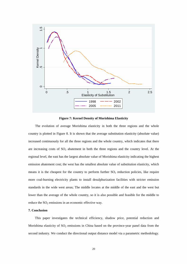
Figure 7 plots the kernel density curves of Morishima elasticity for different provinces in
1998, 2002, 2005 and 2011. More detailed estimates of Morishima elasticity are reported in Table
3A appended. The figure shows that the kernel density curves of Morishima elasticity move
rightward smoothly and slowly at the beginning years of the sample selected. From 2005 to 2011,
it shifts rightward significantly, which means that the average absolute value of the substitution
elasticity has increased a lot in this period. In other words, it has become more costly for the
provinces in China to reduce SO2 emissions in the 11th and 12th FYPs.
20
0.5
11.
5K
erne
l Den
sity
0 .5 1 1.5 2 2.5Elasticity of Substitution
1998 20022005 2011
Figure 7: Kernel Density of Morishima Elasticity
The evolution of average Morishima elasticity in both the three regions and the whole
country is plotted in Figure 8. It is shown that the average substitution elasticity (absolute value)
increased continuously for all the three regions and the whole country, which indicates that there
are increasing costs of SO2 abatement in both the three regions and the country level. At the
regional level, the east has the largest absolute value of Morishima elasticity indicating the highest
emission abatement cost; the west has the smallest absolute value of substitution elasticity, which
means it is the cheapest for the country to perform further SO2 reduction policies, like require
more coal-burning electricity plants to install desulphurization facilities with stricter emission
standards in the wide west areas; The middle locates at the middle of the east and the west but
lower than the average of the whole country, so it is also possible and feasible for the middle to
reduce the SO2 emissions in an economic effective way.
7. Conclusion
This paper investigates the technical efficiency, shadow price, potential reduction and
Morishima elasticity of SO2 emissions in China based on the province-year panel data from the
second industry. We conduct the directional output distance model via a parametric methodology.

21
There is one good output, gross industrial product value, and one bad output, SO2 emission. The
net value of fixed, annual average number of employees and energy input comprise the three
different inputs.
0.00
0.50
1.00
1.50
2.00
2.50
3.00
1998 1999 2000 2001 2002 2003 2004 2005 2006 2007 2008 2009 2010 2011
Subs
titut
ion
Elas
ticity
East Middle West China
Figure 8: Average Elasticity of Substitution by Region
Overall we find that technical efficiency is improved in a non-linear form over times, which
implies that the technical efficiency might become higher as time elapsed but returned to lower
level in the next years. The non-linear changing rule could be explained as that the three regions
experience different technical efficiency improvement in the whole process. The technical
efficiency in the east is improved a lot while in the middle it experienced a dispersed U-shape and
it is almost increasing rapidly during the whole period for the west. The three curves intersect
among the years of 2008-2009. Meanwhile, the potential reductions of SO2 in the east and middle
converge to some extent during the whole period, while the west becomes dominated in the SO2
emission reductions.
As regard the shadow price, they keep the similar increasing path in the west and the middle
while the price in the east increased much more and become the most expensive in 2011 at the
beginning of the 12th FYP. Henan and Shandong have the highest level of shadow price of SO2,

22
which indicates that these two provinces encountered the most serious environmental situations. In
China, the levy of SO2 pollution was increased from 0.04 Yuan /kg to 0.21 Yuan /kg in 1998, then
increased to 0.42 Yuan /kg in 2003, 0.63 Yuan /kg in 2004 and crawled to 1.26 Yuan /kg in 2007
(OECD, 2007). Compared with the price estimated in this paper, the pollution levy might be too
lower. The levy rate should be not only increased to the estimated average cost of controlling SO2
emissions, but also should reflect the marginal abatement cost of SO2 emissions.
Besides, the disparities of technical efficiency, shadow price, potential reduction and
Morishima elasticity are significant among the provinces and three regions. It is shown that the
average price of SO2 in China from 1998 to 2011 among all the 30 provinces is 0.69 million Yuan,
the minimum is 0.03 million Yuan which occurred in Shandong in 1999 and the maximum of the
price also appeared in Shandong but in 2011, which is 11.67 million Yuan. Meanwhile, the east
has the largest absolute value of Morishima elasticity, the west has the smallest absolute value of
substitution elasticity and the middle locates at the middle of the east and the west. What all these
results imply that the diversified prices among the provinces and regions are essential for
constructing a country/province wide market, and the different difficulties in SO2 emission
reductions have important implications for the central government to allocate the abatement
responsibilities among the provinces or regions in the near future.
Reference
Aigner, D.J., Chu, S.F., “On estimating the industry production function”. American Economic
Review, 1968, 58, 826-839.
Atkinson, S.E, and J. H. Dorfman, “Bayesian measurement of productivity and efficiency in the
presence of undesirable outputs: crediting electric utilities for reducing air pollution”,
Journal of Econometrics, 2005, 126(2), 445-468.
Boyd, G., J. Molburg, and R. Prince. Alternative methods of marginal abatement cost estimation:
Nonparametric distance functions, Paper presented at the 17thAnnualNorthAmerican
Conference of the United States Association for Energy Economics and the International
Association for Energy Economics, 1996. October 27–30,Boston.
Chambers, R., Chung, Y., Färe, R., “Profit, directional distance functions, and Nerlovian
efficiency”. Journal of Optimization Theory and Applications, 1998, 98, 351-364.
Chung,Y., R. Färe, and S. Grosskopf, “Productivity and Undesirable Outputs: A Directional
Distance Function Approach”, Journal of Environmental Management, 1997, 51, 229–240.
CMA. “The smog days in March 2013 have been the most since 1961 in China”, 2-4-2014

23
<http://www.gov.cn/jrzg/2013-04/02/content_2368790.htm>
Coggins, J.S., and J. R. Swinton, “The Price of Pollution: A Dual Approach to Valuing SO2
Allowances”, Journal of Environmental Economics and Management, 1996, 30(1), 58-72.
Du, L.M., A. Hanley, C. Wei, “Estimating the marginal abatement costs of carbon dioxide
emissions in China: A parametric analysis”, Kiel Working Papers, 2013, 1883, <
http://www.ifw-members.ifw-kiel.de/publications/estimating-the-marginal-abatement-costs
-of-carbon-dioxide-emissions-in-china-a-parametric-analysis/KWP_1883.pdf>.
Färe, R., S. Grosskopf, C. A. K. Lovell, et al., “Derivation of Shadow Prices for Undesirable
Outputs: A Distance Function Approach”, The Review of Economics and Statistics, 1993,
75(2), 374-380.
Färe, R., S. Grosskopf, D.W. Nohb, et al., “Characteristics of a polluting technology: theory and
practice”, Journal of Econometrics, 2005, 126, 469–492.
Färe, R., Grosskopf, S., Weber, W.L., “Shadow prices and pollution costs in U.S. agriculture”.
Ecological Economics, 2006, 56, 89-103.
Gollop, M., and M.J. Roberts, “Cost-Minimizing Regulation of Sulfur Emissions: Regional Gains
in Electric Power.” Review of Economics and Statistics, 1985, 67, 81-90.
Hao, J., K. He, L. Duan, et al., Air pollution and its control in China. Frontiers of Environmental
Science & Engineering in China, 2007, 1 (2), 129–142.
Kanada, M., L. Dong, T. Fujita, et al., “Regional disparity and cost-effective SO2 pollution control
in China: A case study in 5 mega-cities”, Energy Policy, 2013,
http://dx.doi.org/10.1016/j.enpol.2013.05.105i.
Kaneko, S., Fujii, H., Sawazu, N., et al., “Financial allocation strategy for the regional pollution
abatement cost of reducing sulfur dioxide emissions in the thermal power sector in China”.
Energy Policy, 2010, 38, 2131-2141.
Ke, T.-Y., Hu, J.-L., Li, Y., et al., “Shadow prices of SO2 abatements for regions in China”.
Agricultural and Resources Economics,2008, 5, 59-78.
Kuosmanen, T., “Representation theorem for convex nonparametric least squares”, Economic
Journal, 2008, 11, 308-325.
Kuosmanen, T., Kortelainen, M., “Stochastic non-smooth envelopment of data semi-parametric
frontier estimation subject to shape constraints”, Journal of product analysis, 2012, 38(1),
11-28.
Lee, J.D., J.B. Park, and T.Y. Kim, “Estimation of the shadow prices of pollutants with
production/environment inefficiency taken into account: a nonparametric directional
distance function approach”, Journal of Environmental Management, 2002, 64, 365–375.
Marklund, P.-O., Samakovlis, E., “What is driving the EU burden-sharing agreement: Efficiency
or equity?” Journal of Environmental Management, 2007, 85, 317-329.
Mekaroonreung, M., A.L. Johnson, “Estimating the shadow prices of SO2 and NOX for U.S. coal
power plants: A convex nonparametric least squares approach”, Energy Economics, 2012,
34, 723-732.
MEP. “China Environment Bulletin 2012”, 6-6-2013,
<http://jcs.mep.gov.cn/hjzl/zkgb/2012zkgb/201306/t20130606_253402.htm>.
Murty, M., Kumar, S., Dhavala, K., “Measuring environmental efficiency of industry: a case study

24
of thermal power generation in India”. Environmental and Resource Economics, 2007, 38,
31-50.
NASA. “Thick smog over China”, 1. Feb. 2006,
<http://visibleearth.nasa.gov/view.php?id=75205>.
NBS,. “China Statistical Yearbook 2004”. China Statistics Press, Beijing 2004.
OECD, OECD Environmental Performance Reviews: China 2007. OECD Publications, Paris,
2007.
Pathak, R.K., W.S. Wu, T. Wang, “Summer time PM2.5 ionic species in four major cities of China:
nitrate formation in an ammonia-deficient atmosphere”. Atmospheric Chemistry and
Physics, 2009, 9(5), 1711–1722.
Salnykov, M., and V. Zelenyuk, Estimation of Environmental Efficiencies of Economies and
Shadow Prices of Pollutants in Countries in Transition. EERC Working Paper
Series05-06e, EERC Research Network, Russia and CIS, 2004.
Schreifels, J.J., Y. Fu, E.J. Wilson, “Sulfur dioxide control in China: policy evolution during the
10th and 11th Five-year Plans and lessons for the future”, Energy policy, 2012, 48, 779-789.
Swinton, R., “At What Cost do We Reduce Pollution? Shadow Prices of SO2 Emissions”, The
Energy Journal, 1998, 19, 63-83.
Tu, Z.G., “The shadow price of industrial SO2 emission: A new analytic framework”, China
Economic Quarterly-in Chinese, 2009, 9(1), 259-282.
Vardanyan, M., Noh, D.-W., “Approximating pollution abatement costs via alternative
specifications of a multi-output production technology: a case of the US electric utility
industry”. Journal of Environmental Management, 2006, 80, 177-190.
Wang, S.X., Hao, J.M., “Air quality management in China: Issues, challenges, and options”.
Journal of Environmental Science-China, 2012, 24, 2–13.
Wang, J., Y. Lei, J. Yang, et al., “China's air pollution control calls for sustainable strategy for the
use of coal”. Environmental Science & Technology, 2012, 46, 4263–4264.
Wei, C., Andreas, L., Liu, B., “An empirical analysis of the CO2 shadow price in Chinese thermal
power enterprises”. Energy Economics, 2013, 40, 22-31.
Wei, J., X. Guo, D. Marinova, et al., “Industrial SO2 pollution and agricultural losses in China:
evidence form heavy air polluters”. Journal of Cleaner Production, 2014, 64, pp404-413.
Wen, J., 2011. Report on the Work of the Government (in Chinese).
Yuan, X.L., M. Mi, R.M. Mu, et al. “Strategic route map of sulphur dioxide reduction in China,”
Energy policy, 2013, 60, 844-851.