estimating unknown sparsity in compressed sensing - journal of

Estimating Unknown Sparsity in Compressed Sensing

Miles E. Lopes [email protected]

UC Berkeley, Dept. Statistics, 367 Evans Hall, Berkeley, CA 94720-3860

Abstract

In the theory of compressed sensing (CS), thesparsity ‖x‖0 of the unknown signal x ∈ Rpis commonly assumed to be a known parame-ter. However, it is typically unknown in prac-tice. Due to the fact that many aspects ofCS depend on knowing ‖x‖0, it is importantto estimate this parameter in a data-drivenway. A second practical concern is that ‖x‖0is a highly unstable function of x. In partic-ular, for real signals with entries not exactlyequal to 0, the value ‖x‖0 = p is not a usefuldescription of the effective number of coordi-nates. In this paper, we propose to estimate astable measure of sparsity s(x) := ‖x‖21/‖x‖22,which is a sharp lower bound on ‖x‖0. Ourestimation procedure uses only a small num-ber of linear measurements, does not rely onany sparsity assumptions, and requires verylittle computation. A confidence interval fors(x) is provided, and its width is shown tohave no dependence on the signal dimensionp. Moreover, this result extends naturally tothe matrix recovery setting, where a soft ver-sion of matrix rank can be estimated withanalogous guarantees. Finally, we show thatthe use of randomized measurements is essen-tial to estimating s(x). This is accomplishedby proving that the minimax risk for estimat-ing s(x) with deterministic measurements islarge when n� p.

1. Introduction

The central problem of compressed sensing (CS) is toestimate an unknown signal x ∈ Rp from n linear mea-surements y = (y1, . . . , yn) given by

y = Ax+ ε, (1)

Proceedings of the 30 th International Conference on Ma-chine Learning, Atlanta, Georgia, USA, 2013. JMLR:W&CP volume 28. Copyright 2013 by the author(s).

where A ∈ Rn×p is a user-specified measurement ma-trix, ε ∈ Rn is a random noise vector, and n is muchsmaller than the signal dimension p. During the lastseveral years, the theory of CS has drawn widespreadattention to the fact that this seemingly ill-posed prob-lem can be solved reliably when x is sparse — inthe sense that the parameter ‖x‖0 := card{j : xj 6= 0}is much less than p. For instance, if n is approxi-mately ‖x‖0 log(p/‖x‖0), then accurate recovery canbe achieved with high probability when A is drawnfrom a Gaussian ensemble (Donoho, 2006; Candeset al., 2006). Along these lines, the value of the pa-rameter ‖x‖0 is commonly assumed to be known inthe analysis of recovery algorithms — even though itis typically unknown in practice. Due to the funda-mental role that sparsity plays in CS, this issue hasbeen recognized as a significant gap between theoryand practice by several authors (Ward, 2009; Eldar,2009; Malioutov et al., 2008). Nevertheless, the liter-ature has been relatively quiet about the problems ofestimating this parameter and quantifying its uncer-tainty.

1.1. Motivations and the role of sparsity

At a conceptual level, the problem of estimating ‖x‖0is quite different from the more well-studied prob-lems of estimating the full signal x or its support setS := {j : xj 6= 0}. The difference arises from sparsityassumptions. On one hand, a procedure for estimating‖x‖0 should make very few assumptions about sparsity(if any). On the other hand, methods for estimatingx or S often assume that a sparsity level is given, andthen impose this value on the solution x or S. Con-sequently, a simple plug-in estimate of ‖x‖0, such as

‖x‖0 or card(S), may fail when the sparsity assump-

tions underlying x or S are invalid.

To emphasize that there are many aspects of CS thatdepend on knowing ‖x‖0, we provide several examplesbelow. Our main point here is that a method for esti-mating ‖x‖0 is valuable because it can help to addressa broad range of issues.


• Modeling assumptions. One of the core mod-eling assumptions invoked in applications of CSis that the signal of interest has a sparse rep-resentation. Likewise, the problem of checkingwhether or not this assumption is supported bydata has been an active research topic, partic-ularly in in areas of face recognition and imageclassification (Rigamonti et al., 2011; Shi et al.,

2011). In this type of situation, an estimate ‖x‖0that does not rely on any sparsity assumptions isa natural device for validating the use of sparserepresentations.

• The number of measurements. If the choiceof n is too small compared to the “critical” num-ber n∗(x) := ‖x‖0 log(p/‖x‖0), then there areknown information-theoretic barriers to the ac-curate reconstruction of x (Arias-Castro et al.,2011). At the same time, if n is chosen to be muchlarger than n∗(x), then the measurement processis wasteful, as there are known algorithms thatcan reliably recover x with approximately n∗(x)measurements (Davenport et al., 2011).

To deal with the selection of n, a sparsity esti-

mate ‖x‖0 may be used in two different ways, de-pending on whether measurements are collectedsequentially, or in a single batch. In the sequentialcase, an estimate of ‖x‖0 can be computed froma set of “preliminary” measurements, and then

the estimated value ‖x‖0 determines how manyadditional measurements should be collected torecover the full signal. Also, it is not always nec-essary to take additional measurements, since thepreliminary set may be re-used to compute x (asdiscussed in Section 5). Alternatively, if all of themeasurements must be taken in one batch, the

value ‖x‖0 can be used to certify whether or notenough measurements were actually taken.

• The measurement matrix. Two of the mostwell-known design characteristics of the matrix Aare defined explicitly in terms of sparsity. Theseare the restricted isometry property of order k(RIP-k), and the restricted null-space property oforder k (NSP-k), where k is a presumed upperbound on the sparsity level of the true signal.Since many recovery guarantees are closely tiedto RIP-k and NSP-k, a growing body of work hasbeen devoted to certifying whether or not a givenmatrix satisfies these properties (d’Aspremont &El Ghaoui, 2011; Juditsky & Nemirovski, 2011;Tang & Nehorai, 2011). When k is treated asgiven, this problem is already computationallydifficult. Yet, when the sparsity of x is unknown,

we must also remember that such a “certificate”is not meaningful unless we can check that k isconsistent with the true signal.

• Recovery algorithms. When recovery al-gorithms are implemented, the sparsity levelof x is often treated as a tuning parame-ter. For example, if k is a presumed boundon ‖x‖0, then the Orthogonal Matching Pur-suit algorithm (OMP) is typically initialized torun for k iterations. A second example isthe Lasso algorithm, which computes the so-lution x ∈ argmin{‖y −Av‖22 + λ‖v‖1 : v ∈ Rp},for some choice of λ ≥ 0 . The sparsity of x isdetermined by the size of λ, and in order to se-lect the appropriate value, a family of solutionsis examined over a range of λ values. In the case

of either OMP or Lasso, a sparsity estimate ‖x‖0would reduce computation by restricting the pos-sible choices of λ or k, and it would also ensurethat the chosen values conform to the true signal.

1.2. An alternative measure of sparsity

Despite the important theoretical role of the param-eter ‖x‖0 in many aspects of CS, it has the practicaldrawback of being a highly unstable function of x. Inparticular, for real signals x ∈ Rp whose entries are notexactly equal to 0, the value ‖x‖0 = p is not a usefuldescription of the effective number of coordinates.

In order to estimate sparsity in a way that accountsfor the instability of ‖x‖0, it is desirable to replacethe `0 norm with a “soft” version. More precisely,we would like to identify a function of x that can beinterpreted like ‖x‖0, but remains stable under smallperturbations of x. A natural quantity that serves thispurpose is the numerical sparsity

s(x) :=‖x‖21‖x‖22

, (2)

which always satisfies 1 ≤ s(x) ≤ p for any non-zerox. Although the ratio ‖x‖21/‖x‖22 appears sporadicallyin different areas (Tang & Nehorai, 2011; Hurley &Rickard, 2009; Hoyer, 2004; Lopes et al., 2011), it doesnot seem to be well known as a sparsity measure in CS.

A key property of s(x) is that it is a sharp lower boundon ‖x‖0 for all non-zero x,

s(x) ≤ ‖x‖0, (3)

which follows from applying the Cauchy-Schwarz in-equality to the relation ‖x‖1 = 〈x, sgn(x)〉. (Equalityin (3) is attained iff the non-zero coordinates of x are


equal in magnitude.) We also note that this inequal-ity is invariant to scaling of x, since s(x) and ‖x‖0 areindividually scale invariant. In the opposite direction,it is easy to see that the only continuous upper boundon ‖x‖0 is the trivial one: If a continuous function fsatisfies ‖x‖0 ≤ f(x) ≤ p for all x in some open subsetof Rp, then f must be identically equal to p. (There isa dense set of points where ‖x‖0 = p.) Therefore, wemust be content with a continuous lower bound.

The fact that s(x) is a sensible measure of sparsityfor non-idealized signals is illustrated in Figure 1. Inessence, if x has k large coordinates and p − k smallcoordinates, then s(x) ≈ k, whereas ‖x‖0 = p. Inthe left panel, the sorted coordinates of three differentvectors in R100 are plotted. The value of s(x) for eachvector is marked with a triangle on the x-axis, whichshows that s(x) adapts well to the decay profile. Thisidea can be seen in a more geometric way in the mid-dle and right panels, which plot the the sub-level setsSc := {x ∈ Rp : s(x) ≤ c} with c ∈ [1, p]. When c ≈ 1,the vectors in Sc are closely aligned with the coordi-nate axes, and hence contain one effective coordinate.As c ↑ p, the set Sc includes more dense vectors untilSp = Rp.

1.3. Related work.

Some of the challenges described in Section 1.1 can beapproached with the general tools of cross-validation(CV) and empirical risk minimization (ERM). Thisapproach has been used to select various parameters,such as the number of measurements n (Malioutovet al., 2008; Ward, 2009), the number of OMP it-erations k (Ward, 2009), or the Lasso regularizationparameter λ (Eldar, 2009). At a high level, these

methods consider a collection of (say m) solutionsx(1), . . . , x(m) obtained from different values θ1, . . . , θmof some tuning parameter of interest. For each so-lution, an empirical error estimate err(x(j)) is com-puted, and the value θj∗ corresponding to the smallesterr(x(j)) is chosen.

Although methods based on CV/ERM share commonmotivations with our work here, these methods dif-fer from our approach in several ways. In particular,the problem of estimating a soft measure of sparsity,such as s(x), has not been considered from that angle.Also, the cited methods do not give any theoreticalguarantees to ensure that the estimated sparsity levelis close to the true one. Note that even if an estimatex has small error ‖x−x‖2, it is not necessary for ‖x‖0to be close to ‖x‖0. This point is especially relevantwhen one is interested in identifying a set of importantvariables or interpreting features.

From a computational point view, the CV/ERM ap-proaches can also be costly — since x(j) is typicallycomputed from a separate optimization problem forfor each choice of the tuning parameter. By contrast,our method for estimating s(x) requires no optimiza-tion, and can be computed easily from just a small setof preliminary measurements.

1.4. Our contributions.

The primary contribution of this paper is our treat-ment of unknown sparsity as a parameter estimationproblem. Specifically, we identify a stable measure ofsparsity that is relevant to CS, and propose an efficientestimator with provable guarantees. Secondly, we arenot aware of any other papers that have demonstrateda distinction between random and deterministic mea-

0 20 40 60 80 100

0.0

0.2

0.4

0.6

0.8

1.0

vectors in R100 and s(x) values

coordinate index

coordinate

value

s(x) = 16.4, ‖x‖0 = 100s(x) = 32.7, ‖x‖0 = 45s(x) = 66.6, ‖x‖0 = 100

16.4 32.7 66.6-1.0 -0.5 0.0 0.5 1.0

-1.0

-0.5

0.0

0.5

1.0

sub-level set s(x) ≤ 1.1 in R2

x1

x2

-1.0 -0.5 0.0 0.5 1.0

-1.0

-0.5

0.0

0.5

1.0

sub-level set s(x) ≤ 1.9 in R2

x1

x2

Figure 1. Characteristics of s(x). Left panel: Three vectors (red, blue, black) in R100 have been plotted with theircoordinates in order of decreasing size (maximum entry normalized to 1). Two of the vectors have power-law decayprofiles, and one is a dyadic vector with exactly 45 positive coordinates (red: xi ∝ i−1, blue: dyadic, black: xi ∝ i−1/2).Color-coded triangles on the bottom axis indicate that the s(x) value represents the “effective” number of coordinates.


surements with regard to unknown sparsity (as in Sec-tion 4).

The remainder of the paper is organized as follows. InSection 2, we show that a principled choice of n canbe made if s(x) is known. This is accomplished byformulating a recovery condition for the Basis Pursuitalgorithm directly in terms of s(x). Next, in Section 3,we propose an estimator s(x), and derive a dimension-free confidence interval for s(x). The procedure is alsoshown to extend to the problem of estimating a softmeasure of rank for matrix-valued signals. In Section 4we show that the use of randomized measurements isessential to estimating s(x). Finally, we present simu-lations in Section 5 to validate the consequences of ourtheoretical results. Due to space constraints, we deferall of our proofs to the supplement.

Notation. We define ‖x‖qq :=∑pj=1 |xj |q for any q >

0 and x ∈ Rp, which only corresponds to a genuinenorm for q ≥ 1. For sequences of numbers an and bn,we write an . bn or an = O(bn) if there is an absoluteconstant c > 0 such that an ≤ cbn for all large n. Ifan/bn → 0, we write an = o(bn). For a matrix M , we

define the Frobenius norm ‖M‖F =√∑

i,jM2ij , the

matrix `1-norm ‖M‖1 =∑i,j |Mij |. Finally, for two

matrices A and B of the same size, we define the innerproduct 〈A,B〉 := tr(A>B).

2. Recovery conditions in terms of s(x)

The purpose of this section is to present a simpleproposition that links s(x) with recovery conditionsfor the Basis Pursuit algorithm (BP). This is an im-portant motivation for studying s(x), since it impliesthat if s(x) can be estimated well, then n can be cho-sen appropriately. In other words, we offer an adaptivechoice of n.

In order to explain the connection between s(x) andrecovery, we first recall a standard result (Candeset al., 2006) that describes the `2 error rate of theBP algorithm. Informally, the result assumes thatthe noise is bounded as ‖ε‖2 ≤ ε0 for some con-stant ε0 > 0, the matrix A ∈ Rn×p is drawn froma suitable ensemble, and n satisfies n & T log(pe/T )for some T ∈ {1, . . . , p} with e = exp(1). Theconclusion is that with high probability, the solutionx ∈ argmin{‖v‖1 : ‖Av − y‖2 ≤ ε0, v ∈ Rp} satisfies

‖x− x‖2 ≤ c1 ε0 + c2‖x−xT ‖1√

T, (4)

where xT ∈ Rp is the best T -term approximation1 to

1The vector xT ∈ Rp is obtained by setting to 0 allcoordinates of x except the T largest ones (in magnitude).

x, and c1, c2 > 0 are constants. This bound is a fun-damental point of reference, since it matches the mini-max optimal rate under certain conditions (Candes,2006), and applies to all signals x ∈ Rp (ratherthan just k-sparse signals). Additional details may befound in (Cai et al., 2010) [Theorem 3.3], (Vershynin,2010) [Theorem 5.65].

We now aim to answer the question, “If s(x) wereknown, how large should n be in order for x to be closeto x?” Since the bound (4) assumes n & T log(pe/T ),our question amounts to choosing T . For this purpose,it is natural to consider the relative `2 error

‖x−x‖2‖x‖2 ≤ c1 ε0

‖x‖2 + c21√T

‖x−xT ‖1‖x‖2 , (5)

so that the T -term approximation error 1√T

‖x−xT ‖1‖x‖2

does not depend on the scale of x (i.e. invariant underx 7→ cx with c 6= 0).

Proposition 1 below shows how knowledge of s(x) al-lows us to control the approximation error. Specifi-cally, the result shows that the condition T & s(x) isnecessary for the approximation error to be small, andthe condition T & s(x) log(p) is sufficient.

Proposition 1. Let x ∈ Rp \{0}, and T ∈ {1, . . . , p}.The following statements hold for any c0, ε > 0.

(i) If the T -term approximation error satisfies1√T

‖x−xT ‖1‖x‖2 ≤ ε, then

T ≥ 1(1+ε)2 · s(x).

(ii) If T ≥ c0 s(x) log(p), then the T -term approxi-mation error satisfies

1√T

‖x−xT ‖1‖x‖2 ≤ 1√

c0 log(p)

(1− T

p

).

In particular, if T ≥ 2s(x) log(p) with p ≥ 100,then

1√T

‖x−xT ‖1‖x‖2 ≤ 1

3 .

Remarks. A notable feature of these bounds isthat they hold for all non-zero signals. In our sim-ulations in Section 5, we show that choosing n =2ds(x)e log(p/ds(x)e) based on an estimate s(x) leadsto accurate reconstruction across many sparsity levels.

3. Estimation results for s(x)

In this section, we give a simple procedure to estimates(x) for any x ∈ Rp \ {0}. The procedure uses a smallnumber of measurements, makes no sparsity assump-tions, and requires very little computation. The mea-surements we prescribe may also be re-used to recoverthe full signal after s(x) has been estimated.


The results in this section are based on the measure-ment model (1), written in scalar notation as

yi = 〈ai, x〉+ εi, i = 1, . . . , n. (6)

We assume only that the noise variables εi are inde-pendent, and bounded by |εi| ≤ σ0, for some constantσ0 > 0. No additional structure on the noise is needed.

3.1. Sketching with stable laws

Our estimation procedure derives from a techniqueknown as sketching in the streaming computation lit-erature (Indyk, 2006). Although this area deals withproblems that have mathematical connections to CS,the use of sketching techniques in CS does not seem tobe well known.

For any q ∈ (0, 2], the sketching technique offers away to estimate ‖x‖q from a set of randomized lin-ear measurements. In our approach, we estimates(x) = ‖x‖21/‖x‖22 by estimating ‖x‖1 and ‖x‖2 fromseparate sets of measurements. The core idea is togenerate the measurement vectors ai ∈ Rp using sta-ble laws (Zolotarev, 1986).

Definition 1. A random variable V has a symmet-ric stable distribution if its characteristic function isof the form E[exp(

√−1tV )] = exp(−|γt|q) for some

q ∈ (0, 2] and some γ > 0. We denote the distribu-tion by V ∼ Sq(γ), and γ is referred to as the scaleparameter.

The most well-known examples of symmetric stablelaws are the cases of q = 2, 1, namely the Gaussiandistribution N(0, γ2) = S2(γ), and the Cauchy dis-tribution C(0, γ) = S1(γ). To fix some notation, ifa vector a1 = (a1,1, . . . , a1,p) ∈ Rp has i.i.d. entriesdrawn from Sq(γ), we write a1 ∼ Sq(γ)⊗p. The con-nection with `q norms hinges on the following propertyof stable distributions (Zolotarev, 1986).

Lemma 1. Suppose x ∈ Rp, and a1 ∼ Sq(γ)⊗p withparameters q ∈ (0, 2] and γ > 0. Then, the randomvariable 〈x, a1〉 is distributed according to Sq(γ‖x‖q).

Using this fact, if we generate a set of i.i.d. vectorsa1, . . . , an from Sq(γ)⊗p and let yi = 〈ai, x〉, theny1, . . . , yn is an i.i.d.sample from Sq(γ‖x‖q). Hence, inthe special case of noiseless linear measurements, thetask of estimating ‖x‖q is equivalent to a well-studiedunivariate problem: estimating the scale parameter ofa stable law from an i.i.d. sample.

When the yi are corrupted with noise, our analysisshows that standard estimators for scale parametersare only moderately affected. The impact of the noisecan also be reduced via the choice of γ when generating

ai ∼ Sq(γ)⊗p. The γ parameter controls the “energylevel” of the measurement vectors ai. (Note that in theGaussian case, if a1 ∼ S2(γ)⊗p, then E‖a1‖22 = γ2p.)In our results, we leave γ as a free parameter to showhow the effect of noise is reduced as γ is increased.

3.2. Estimation procedure for s(x)

Two sets of measurements are used to estimate s(x),and we write the total number as n = n1 + n2. Thefirst set is obtained by generating i.i.d. measurementvectors from a Cauchy distribution,

ai ∼ C(0, γ)⊗p, i = 1, . . . , n1. (7)

The corresponding values yi are then used to estimate‖x‖1 via the statistic

T1 := 1γmedian(|y1|, . . . , |yn1

|), (8)

which is a standard estimator of the scale parameter ofthe Cauchy distribution (Fama & Roll, 1971; Li et al.,2007). Next, a second set of i.i.d.measurement vectorsare generated from a Gaussian distribution

ai ∼ N(0, γ2)⊗p, i = n1 + 1, . . . , n1 +n2. (9)

In this case, the associated yi values are used to com-pute an estimate of ‖x‖22 given by

T 22 := 1

γ2n2(y2n1+1 + · · ·+ y2n1+n2

), (10)

which is a natural estimator of the variance of a Gaus-sian distribution. Combining these two statistics, ourestimate of s(x) = ‖x‖21/‖x‖22 is defined as

s(x) := T 21

/T 22 . (11)

3.3. Confidence interval.

The following theorem describes the relative error∣∣ s(x)s(x)−1

∣∣ via an asymptotic confidence interval for s(x).

Our result is stated in terms of the noise-to-signal ratio

ρ := σ0

γ‖x‖2 ,

and the standard Gaussian quantile z1−α, which satis-fies Φ(z1−α) = 1− α for any coverage level α ∈ (0, 1).In this notation, the following parameters govern thewidth of the confidence interval,

ηn(α, ρ) := z1−α√n

+ ρ and δn(α, ρ) := πz1−α√2n

+ ρ,

and we write these simply as δn and ηn. As is standardin high-dimensional statistics, we allow all of the modelparameters p, x, σ0 and γ to vary implicitly as func-tions of (n1, n2), and let (n1, n2, p)→∞. For simplic-ity, we choose to take measurement sets of equal sizes,


n1 = n2 = n/2, and we place a mild constraint on ρ,namely ηn(α, ρ) < 1. (Note that standard algorithmssuch as Basis Pursuit are not expected to perform wellunless ρ � 1, as is clear from the bound (5).) Lastly,we make no restriction on the growth of p/n, whichmakes s(x) well-suited to high-dimensional problems.

Theorem 1. Let α ∈ (0, 1/2) and x ∈ Rp \ {0}. As-sume that s(x) is constructed as above, and that themodel (6) holds. Suppose also that n1 = n2 = n/2 andηn(α, ρ) < 1 for all n. Then as (n, p)→∞, we have

P(√

s(x)s(x) ∈

[1−δn1+ηn

, 1+δn1−ηn])≥ (1− 2α)2 + o(1). (12)

Remarks. The most important feature of this resultis that the width of the confidence interval does notdepend on the dimension or sparsity of the unknownsignal. Concretely, this means that the number of mea-surements needed to estimate s(x) to a fixed precisionis only O(1) with respect to the size of the problem.Our simulations in Section 5 also show that the relativeerror of s(x) does not depend on dimension or sparsityof x. Lastly, when δn and ηn are small, we note thatthe relative error |s(x)/s(x) − 1| is at most of order(n−1/2 + ρ) with high probability, which follows from

the simple Taylor expansion (1+ε)2

(1−ε)2 = 1 + 4ε+ o(ε).

3.4. Estimating rank and sparsity of matrices

The framework of CS naturally extends to the problemof recovering an unknown matrix X ∈ Rp1×p2 on thebasis of the measurement model

y = A(X) + ε, (13)

where y ∈ Rn, A is a user-specified linear operatorfrom Rp1×p2 to Rn, and ε ∈ Rn is a vector of noisevariables. In recent years, many researchers have ex-plored the recovery of X when it is assumed to havesparse or low rank structure. We refer to the pa-pers (Candes & Plan, 2011; Chandrasekaran et al.,2010) for descriptions of numerous applications. Inanalogy with the previous section, the parametersrank(X) or ‖X‖0 play important theoretical roles, butare very sensitive to perturbations of X. Likewise, itis of basic interest to estimate stable measures of rankand sparsity for matrices. Since the sparsity analogues(X) := ‖X‖21/‖X‖2F can be estimated as a straight-forward extension of Section 3.2, we restrict our atten-tion to the more distinct problem of rank estimation.

3.4.1. The rank of semidefinite matrices

In the context of recovering a low-rank positivesemidefinite matrix X ∈ Sp×p+ \{0}, the quantity

rank(X) plays the role of ‖x‖0 in the recovery of asparse vector. If we let λ(X) ∈ Rp+ denote the vec-tor of ordered eigenvalues of X, the connection canbe made explicit by writing rank(X) = ‖λ(X)‖0. Asin Section 3.2, our approach is to consider a robustalternative to the rank. Motivated by the quantitys(x) = ‖x‖21

/‖x‖22 in the vector case, we now consider

r(X) :=‖λ(X)‖21‖λ(X)‖22

= tr(X)2

‖X‖2F

as our measure of the effective rank for non-zero X,which always satisfies 1 ≤ r(X) ≤ p. The quan-tity r(X) has appeared elsewhere as a measure ofrank (Lopes et al., 2011; Tang & Nehorai, 2010), butis less well known than other rank relaxations, such asthe numerical rank ‖X‖2F

/‖X‖2op (Rudelson & Ver-

shynin, 2007). The relationship between r(X) andrank(X) is completely analogous to s(x) and ‖x‖0.Namely, we have a sharp, scale-invariant inequality

r(X) ≤ rank(X).

The quantity r(X) is more stable than rank(X) in thesense that if X has k large eigenvalues, and p−k smalleigenvalues, then r(X) ≈ k, whereas rank(X) = p.

Our procedure for estimating r(X) is based on esti-mating tr(X) and ‖X‖2F from separate sets of measure-ments. The semidefinite condition is exploited throughthe basic relation 〈Ip×p, X〉 = tr(X) = ‖λ(X)‖1. Toestimate tr(X), we use n1 linear measurements of theform

yi = 〈γIp×p, X〉+ εi, i = 1, . . . , n1 (14)

and compute the estimator T1 := 1γ

1n1

∑n1

i=1 yi, whereγ > 0 is again the measurement energy parameter.Next, to estimate ‖X‖2F , we note that if Z ∈ Rp×p hasi.i.d. N(0, 1) entries, then E〈X,Z〉2 = ‖X‖2F . Hence,if we collect n2 additional measurements of the form

yi = 〈γZi, X〉+ εi, i = n1 + 1, . . . , n1 + n2, (15)

where the Zi ∈ Rp×p are independent random matriceswith i.i.d. N(0, 1) entries, then a suitable estimatorof ‖X‖2F is T 2

2 := 1γ2n2

∑n1+n2

i=n1+1 y2i . Combining these

statistics, we propose

r(X) := T 21

/T 22

as our estimate of r(X). In principle, this procedurecan be refined by using the measurements (14) to esti-mate the noise distribution, but we omit these details.Also, we retain the assumptions of the previous sec-tion, and assume only that the εi are independent andbounded by |εi| ≤ σ0. The next theorem shows thatthe estimator r(X) mirrors s(X) as in Theorem 1, butwith ρ being replaced by % := σ0

/(γ‖X‖F ), and with

ηn being replaced by ζn = ζn(%, α) := z1−α/√n+ %.


Theorem 2. Let α ∈ (0, 1/2) and X ∈ Sp×p+ \ {0}.Assume that r(X) is constructed as above, and that themodel (13) holds. Suppose also that n1 = n2 = n/2and ζn(α, ρ) < 1 for all n. Then as (n, p) → ∞, wehave

P(√

r(X)r(X) ∈

[1−%1+ζn

, 1+%1−ζn

])≥ 1− 2α+ o(1). (16)

Remarks. In parallel with Theorem 1, this confi-dence interval has the valuable property that its widthdoes not depend on the rank or dimension of X, butmerely on the noise-to-signal ratio % = σ0

/(γ‖X‖F ).

The relative error |r(X)/r(X)− 1| is at most of order(n−1/2 + %) with high probability when ζn is small.

4. Deterministic measurement matrices

The problem of constructing deterministic matrices Awith good recovery properties (e.g. RIP-k or NSP-k)has been a longstanding topic within CS. Since ourprocedure in Section 3.2 selects A at random, it isnatural to ask if randomization is essential to the esti-mation of unknown sparsity. In this section, we showthat estimating s(x) with a deterministic matrix Aleads to results that are inherently different from ourrandomized procedure.

At an informal level, the difference between randomand deterministic matrices makes sense if we think ofthe estimation problem as a game between nature anda statistician. Namely, the statistician first chooses amatrix A ∈ Rn×p and an estimation rule δ : Rn → R.(The function δ takes y ∈ Rn as input and returnsan estimate of s(x).) In turn, nature chooses a sig-nal x ∈ Rp \ {0}, with the goal of maximizing thestatistician’s error. When the statistician chooses Adeterministically, nature has the freedom to adversar-ially select an x that is ill-suited to the fixed matrixA. By contrast, if the statistician draws A at random,then nature does not know what value A will take, andtherefore has less knowledge to choose a “bad” signal.

In the case of noiseless random measurements,Theorem 1 implies that our particular estimationrule s(x) can achieve a relative error of order|s(x)/s(x)− 1| = O(n−1/2) with high probability forany non-zero x. (cf. Remarks for Theorem 1.) Ouraim is now to show that for noiseless deterministicmeasurements, all estimation rules δ have a worst-caserelative error |δ(Ax)/s(x)−1| that is much larger thanthan n−1/2. In other words, there is always a choice ofx that can defeat a deterministic procedure, whereass(x) is likely to succeed under any choice of x.

In stating the following result, we note that it involvesno randomness whatsoever — since we assume that

the observed measurements y = Ax are noiseless andobtained from a deterministic matrix A.

Theorem 3. The minimax relative error for estimat-ing s(x) from noiseless deterministic measurementsy = Ax satisfies

infA∈Rn×p

infδ:Rn→R

supx∈Rp\{0}

∣∣∣ δ(Ax)s(x) − 1∣∣∣ ≥ 1−(n+1)/p

2(1+2√

2 log(2p))2.

Remarks. Under the typical high-dimensional sce-nario where there is some κ ∈ (0,∞) for whichp/n→ κ as (n, p) → ∞, we have the lower bound

| δ(Ax)s(x) − 1| & 1log(n) , which is much larger than n−1/2.

5. Simulations

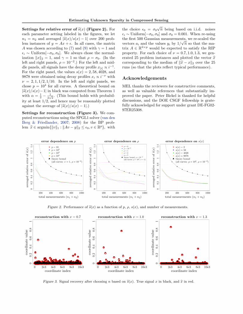
Relative error of s(x). To validate the conse-quences of Theorem 1, we study how the relative error|s(x)/s(x) − 1| depends on the parameters p, ρ, ands(x). We generated measurements y = Ax + ε under

a broad range of parameter settings, with x ∈ R104 inmost cases. Note that although p = 104 is a very largedimension, it is not at all extreme from the viewpointof applications (e.g. a megapixel image with p = 106).Details regarding parameter settings are given below.As anticipated by Theorem 1, the left and right panelsin Figure 2 show that the relative error has no notice-able dependence on p or s(x). The middle panel showsthat for fixed n1 + n2, the relative error grows moder-ately with ρ = σ0

γ‖x‖2 . Lastly, our theoretical bounds

on |s(x)/s(x) − 1| conform to the empirical curves inthe case of low noise (ρ = 10−2).

Reconstruction of x based on s(x). For theproblem of choosing n, we considered the choice ofn := 2ds(x)e log(p/ds(x)e). The simulations show thatn adapts to the structure of the true signal, andis also sufficiently large for accurate reconstruction.First, to compute s(x), we followed Section 3.2, anddrew initial measurement sets of Cauchy and Gaus-sian vectors with n1 = n2 = 500 and γ = 1. Ifit happened to be the case that 500 ≥ n, then re-construction was performed using only the initial 500Gaussian measurements. Alternatively, if n > 500,then (n − 500) additional measurements vectors aiwere drawn from N(0, n−1/2Ip×p) for reconstruction.Further details are given below. Figure 3 illustratesthe results for three power-law signals in R104 withx[i] ∝ i−ν , ν = 0.7, 1.0, 1.3 and ‖x‖1 = 1 (corre-sponding to s(x) = 823, 58, 11). In each panel, thecoordinates of x are plotted in black, and those of xare plotted in red. Clearly, there is good qualitativeagreement in all cases. From left to right, the value ofn = 2ds(x)e log(p/ds(x)e) was 4108, 590, and 150.


Settings for relative error of s(x) (Figure 2). Foreach parameter setting labeled in the figures, we letn1 = n2 and averaged |s(x)/s(x)− 1| over 200 prob-lem instances of y = Ax + ε. In all cases, the matrixA was chosen according to (7) and (9) with γ = 1 andεi ∼ Uniform[−σ0, σ0]. We always chose the normal-ization ‖x‖2 = 1, and γ = 1 so that ρ = σ0. (In theleft and right panels, ρ = 10−2.) For the left and mid-dle panels, all signals have the decay profile x[i] ∝ i−1.For the right panel, the values s(x) = 2, 58, 4028, and9878 were obtained using decay profiles xi ∝ i−ν withν = 2, 1, 1/2, 1/10. In the left and right panels, wechose p = 104 for all curves. A theoretical bound on|s(x)/s(x)−1| in black was computed from Theorem 1with α = 1

2 − 12√2. (This bound holds with probabil-

ity at least 1/2, and hence may be reasonably plottedagainst the average of |s(x)/s(x)− 1|.)Settings for reconstruction (Figure 3). We com-puted reconstructions using the SPGL1 solver (van denBerg & Friedlander, 2007; 2008) for the BP prob-lem x ∈ argmin{‖v‖1 : ‖Av − y‖2 ≤ ε0, v ∈ Rp}, with

the choice ε0 = σ0√n being based on i.i.d. noises

εi ∼ Uniform[−σ0, σ0] and σ0 = 0.001. When re-usingthe first 500 Gaussian measurements, we re-scaled thevectors ai and the values yi by 1/

√n so that the ma-

trix A ∈ Rn×p would be expected to satisfy the RIPproperty. For each choice of ν = 0.7, 1.0, 1.3, we gen-erated 25 problem instances and plotted the vector xcorresponding to the median of ‖x − x‖2 over the 25runs (so that the plots reflect typical performance).

Acknowledgements

MEL thanks the reviewers for constructive comments,as well as valuable references that substantially im-proved the paper. Peter Bickel is thanked for helpfuldiscussions, and the DOE CSGF fellowship is grate-fully acknowledged for support under grant DE-FG02-97ER25308.

error dependence on p

total measurements (n1 + n2)

averaged

relative

errorofs(x)

00.2

0.4

0.6

0.8

11.2

1.4

200 400 600 800 1000

p = 10p = 102

p = 103

p = 104

theory bound(all curves: ν = 1, ρ = 10−2)

error dependence on ρ


averaged

relative

errorofs(x)

00.2

0.4

0.6

0.8

11.2

1.4

200 400 600 800 1000

ρ = 0ρ = 10−2

ρ = 1ρ = 2ρ = 5theory bound, ρ = 10−2

(all curves: p = 104, ν = 1)

error dependence on s(x)


averaged

relative

errorofs(x)

00.2

0.4

0.6

0.8

11.2

1.4

200 400 600 800 1000

s(x) = 2s(x) = 58s(x) = 4028s(x) = 9878theory bound(all curves: p = 104, ρ = 10−2)

Figure 2. Performance of s(x) as a function of p, ρ, s(x), and number of measurements.

reconstruction with ν = 0.7

coordinate index

coordinatevalue

00.2

0.4

0.6

0.8

1

0 2e3 4e3 6e3 8e3 10e3


coordinate index

coordinatevalue

00.2

0.4

0.6

0.8

1

0 2e3 4e3 6e3 8e3 10e3


coordinate index

coordinatevalue

00.2

0.4

0.6

0.8

1

0 2e3 4e3 6e3 8e3 10e3

Figure 3. Signal recovery after choosing n based on s(x). True signal x in black, and x in red.


References

Arias-Castro, E., Candes, E. J., and Davenport, M. On thefundamental limits of adaptive sensing. Arxiv preprintarXiv:1111.4646, 2011.

Cai, T. T., Wang, L., and Xu, G. New bounds for re-stricted isometry constants. Information Theory, IEEETransactions on, 56(9), 2010.

Candes, E. J. Compressive sampling. In Proceedings oh theInternational Congress of Mathematicians: Madrid, Au-gust 22-30, 2006: invited lectures, pp. 1433–1452, 2006.

Candes, E. J. and Plan, Y. Tight oracle inequalities for low-rank matrix recovery from a minimal number of noisyrandom measurements. IEEE Transactions on Informa-tion Theory, 57(4):2342–2359, 2011.

Candes, E. J., Romberg, J.K., and Tao, T. Stable signalrecovery from incomplete and inaccurate measurements.Communications on pure and applied mathematics, 59(8):1207–1223, 2006.

Chandrasekaran, V., Recht, B., Parrilo, P. A., and Willsky,A. S. The convex algebraic geometry of linear inverseproblems. In Communication, Control, and Computing(Allerton), 2010 48th Annual Allerton Conference on,pp. 699–703. IEEE, 2010.

d’Aspremont, A. and El Ghaoui, L. Testing the nullspaceproperty using semidefinite programming. Mathematicalprogramming, 127(1):123–144, 2011.

Davenport, M. A., Duarte, M. F., Eldar, Y. C., and Ku-tyniok, G. Introduction to compressed sensing. Preprint,93, 2011.

Donoho, D. L. Compressed sensing. IEEE Transactionson Information Theory, 52(4):1289–1306, 2006.

Eldar, Y. C. Generalized sure for exponential families:Applications to regularization. IEEE Transactions onSignal Processing, 57(2):471–481, 2009.

Fama, E. F. and Roll, Richard. Parameter estimates forsymmetric stable distributions. Journal of the AmericanStatistical Association, 66(334):331–338, 1971.

Hoyer, P.O. Non-negative matrix factorization with sparse-ness constraints. The Journal of Machine Learning Re-search, 5:1457–1469, 2004.

Hurley, N. and Rickard, S. Comparing measures of spar-sity. IEEE Transactions on Information Theory, 55(10):4723–4741, 2009.

Indyk, P. Stable distributions, pseudorandom generators,embeddings, and data stream computation. Journal ofthe ACM (JACM), 53(3):307–323, 2006.

Juditsky, A. and Nemirovski, A. On verifiable sufficientconditions for sparse signal recovery via `1 minimization.Mathematical programming, 127(1):57–88, 2011.

Li, P., Hastie, T., and Church, K. Nonlinear estimators andtail bounds for dimension reduction in l 1 using cauchyrandom projections. Journal of Machine Learning Re-search, pp. 2497–2532, 2007.

Lopes, M. E., Jacob, L., and Wainwright, M.J. A morepowerful two-sample test in high dimensions using ran-dom projection. In NIPS 24, pp. 1206–1214. 2011.

Malioutov, D. M., Sanghavi, S., and Willsky, A. S. Com-pressed sensing with sequential observations. In IEEEInternational Conference on Acoustics, Speech and Sig-nal Processing, 2008., pp. 3357–3360. IEEE, 2008.

Rigamonti, R., Brown, M. A., and Lepetit, V. Are sparserepresentations really relevant for image classification?In Computer Vision and Pattern Recognition (CVPR),2011 IEEE Conference on, pp. 1545–1552. IEEE, 2011.

Rudelson, M. and Vershynin, R. Sampling from large ma-trices: An approach through geometric functional anal-ysis. Journal of the ACM (JACM), 54(4):21, 2007.

Shi, Q., Eriksson, A., van den Hengel, A., and Shen, C. Isface recognition really a compressive sensing problem?In Computer Vision and Pattern Recognition (CVPR),2011 IEEE Conference on, pp. 553–560. IEEE, 2011.

Tang, G. and Nehorai, A. The stability of low-rank ma-trix reconstruction: a constrained singular value view.arXiv:1006.4088, submitted to IEEE Transactions onInformation Theory, 2010.

Tang, G. and Nehorai, A. Performance analysis of sparserecovery based on constrained minimal singular values.IEEE Transactions on Signal Processing, 59(12):5734–5745, 2011.

van den Berg, E. and Friedlander, M. P. SPGL1: Asolver for large-scale sparse reconstruction, June 2007.http://www.cs.ubc.ca/labs/scl/spgl1.

van den Berg, E. and Friedlander, M. P. Probing thepareto frontier for basis pursuit solutions. SIAM Jour-nal on Scientific Computing, 31(2):890–912, 2008. doi:10.1137/080714488. URL http://link.aip.org/link/?SCE/31/890.

Vershynin, R. Introduction to the non-asymptotic analy-sis of random matrices. Arxiv preprint arxiv:1011.3027,2010.

Ward, R. Compressed sensing with cross validation. IEEETransactions on Information Theory, 55(12):5773–5782,2009.

Zolotarev, V. M. One-dimensional stable distributions, vol-ume 65. Amer Mathematical Society, 1986.

http://link.aip.org/link/?SCE/31/890

http://link.aip.org/link/?SCE/31/890

estimating unknown sparsity in compressed sensing - journal of

Documents