estimatingthepayofftoattendingamore …e.g.,studentsat),andanothersetofvariablesthatis...

ESTIMATING THE PAYOFF TO ATTENDING A MORESELECTIVE COLLEGE: AN APPLICATION OF

SELECTION ON OBSERVABLES AND UNOBSERVABLES*

STACY BERG DALE AND ALAN B. KRUEGER

Estimates of the effect of college selectivity on earnings may be biasedbecause elite colleges admit students, in part, based on characteristics that arerelated to future earnings. We matched students who applied to, and were ac-cepted by, similar colleges to try to eliminate this bias. Using the College andBeyond data set and National Longitudinal Survey of the High School Class of1972, we �nd that students who attended more selective colleges earned about thesame as students of seemingly comparable ability who attended less selectiveschools. Children from low-income families, however, earned more if they at-tended selective colleges.

A burgeoning literature has addressed the question, “Doesthe ‘quality’ of the college that students attend in�uence theirsubsequent earnings?”1 Obtaining accurate estimates of the pay-off to attending a highly selective undergraduate institution is ofobvious importance to the parents of prospective students whofoot the tuition bills, and to the students themselves. In addition,because college selectivity is typically measured by the averagecharacteristics (e.g., average SAT score) of classmates, the litera-ture is closely connected to theoretical and empirical studies ofpeer group effects on individual behavior. And with higher edu-cation making up 40 percent of total educational expenditures inthe United States (see U. S. Department of Education [1997,Table 33]), understanding the impact of selective colleges onstudents’ labor market outcomes is central for understanding therole of human capital.2

* We thank Orley Ashenfelter, Marianne Bertrand, William Bowen, DavidBreneman, David Card, James Heckman, Bo Honore, Thomas Kane, LawrenceKatz, Deborah Peikes, Michael Rothschild, Sarah Turner, colleagues at the Mel-lon Foundation, and three anonymous referees for helpful discussions. We aloneare responsible for any errors in computation or interpretation that may remaindespite their helpful advice. This paper makes use of the College and Beyond(C&B) database. The C&B database is a “restricted access database.” Researcherswho are interested in using the database may apply to the Andrew W. MellonFoundation for access.

1. The modern literature began with papers by Hunt [1963], Solmon [1973],Wales [1973], Solmon and Wachtel [1975], and Wise [1975], and has undergone arecent renaissance, with papers by Brewer and Ehrenberg [1996], Behrman et al.[1996], Daniel, Black, and Smith [1997], Kane [1998], and others. See Brewer andEhrenberg [1996, Table 1] for an excellent summary of the literature.

2. This �gure ignores any earnings students forgo while attending school,which would increase the relative cost of higher education.

© 2002 by the President and Fellows of Harvard College and the Massachusetts Institute ofTechnology.The Quarterly Journal of Economics, November 2002

1491

Past studies have found that students who attended collegeswith higher average SAT scores or higher tuition tend to havehigher earnings when they are observed in the labor market.Attending a college with a 100 point higher average SAT isassociated with 3 to 7 percent higher earnings later in life (see,e.g., Kane [1998]). As Kane notes, an obvious concern with thisconclusion is that students who attend more elite colleges mayhave greater earnings capacity regardless of where they attendschool. Indeed, the very attributes that lead admissions commit-tees to select certain applicants for admission may also be re-warded in the labor market. Most past studies have used Ordi-nary Least Squares (OLS) regression analysis to attempt tocontrol for differences in student attributes that are correlatedwith earnings and college qualities. But college admissions deci-sions are based in part on student characteristics that are unob-served by researchers and therefore not held constant in theestimated wage equations; if these unobserved characteristics arepositively correlated with wages, then OLS estimates will over-state the payoff to attending a selective school. Only three previ-ous papers that we are aware of have attempted to adjust forselection on unobserved variables in estimating the payoff toattending an elite college. Brewer, Eide, and Ehrenberg [1999]use a parametric utility maximizing framework to model stu-dents’ choice of schools, under the assumption that all studentscan attend any school they desire. Behrman, Rosenzweig, andTaubman [1996] utilize data on female twins to difference outcommon unobserved effects, and Behrman et al. [1996] use familyvariables to instrument for college choice. Our paper comple-ments these previous approaches.

This paper employs two new approaches to adjust for non-random selection of students on the part of elite colleges. In oneapproach, we only compare college selectivity and earningsamong students who were accepted and rejected by a comparableset of colleges, and are comparable in terms of observable vari-ables. In the second approach, we hold constant the average SATscore of the schools to which each student applied, as well as theaverage SAT score of the school the student actually attended, thestudent’s own SAT score, and other variables. The second ap-proach is nested in the �rst estimator. Conditions under whichthese estimators provide unbiased estimates of the payoff tocollege quality are discussed in the next section. In short, ifadmission to a college is based on a set of variables that are

1492 QUARTERLY JOURNAL OF ECONOMICS

observed by the admissions committee and later by the econome-trician (e.g., student SAT), and another set of variables that isobserved by the admissions committee (e.g., an assessment ofstudent motivation) but not by the econometrician, and if bothsets of variables in�uence earnings, then looking within matchedsets of students who were accepted and rejected by the samegroups of colleges can help overcome selection bias.

Barnow, Goldberger, and Cain [1981] point out that, “Unbi-asedness is attainable when the variables that determined theassignment rule are known, quanti�ed, and included in the [re-gression] equation.” Our �rst estimator extends their concept of“selection on the observables” to “selection on the observables andunobservables,” since information on the unobservables can beinferred from the outcomes of independent admission decisions bythe schools the student applied to. The general idea of usinginformation re�ected in the outcome of independent screens tocontrol for selection bias may have applications to other estima-tion problems, such as estimating wage differentials associatedwith working in different industries or sizes of �rms (wherehiring decisions during the job search process provide screens)and racial differences in mortgage defaults (where denials oracceptances of applications for loans provide screens).3

We provide selection-corrected estimates of the payoff toschool quality using two data sets: the College and Beyond Sur-vey, which was collected by the Andrew W. Mellon Foundationand analyzed extensively in Bowen and Bok [1998], and theNational Longitudinal Survey of the High School Class of 1972(NLS-72). Two indirect indicators of college quality are used:college selectivity, as measured by a school’s average SAT score,and net tuition. Our primary �nding is that the monetary returnto attending a college with a higher average SAT score fallsconsiderably once we adjust for selection on the part of the col-lege. Nonetheless, we still �nd a substantial payoff to attendingschools with higher net tuition.

Although most of the previous literature has implicitly as-sumed that the returns to attending a selective school are homo-geneous across students, an important issue in interpreting our�ndings is that there may be heterogeneous returns to students

3. Braun and Szatrowski [1984] use a related idea to evaluate law schoolgrades across institutions by comparing the performance of students who wereaccepted at a common set of law schools but attended different schools.

1493ATTENDING A MORE SELECTIVE COLLEGE

for attending the same school. Some students may bene�t morefrom attending a highly selective (or unselective) school thanothers. For example, a student intent on becoming an engineer islikely to have at least as high earnings by attending Pennsylva-nia State University as Williams College, since Williams does nothave an engineering major. In this situation, if students areaware of their own potential returns from each school to whichthey are admitted, they could be expected to sort into schoolsbased on their expected utility from attending that school, as inthe Roy model of occupational choice. In other words, the studentswho chose to go to less selective schools may do so because theyhave higher returns from attending those schools (or becausethere are nonpecuniary bene�ts from attending those schools);however, the average students might not have a higher returnfrom attending a less selective school over a more selective one.Nonetheless, contrary to the previous literature, this interpreta-tion implies that attending a more selective school is not theincome-maximizing choice for all students. Instead, studentswould maximize their returns by attending the school that offersthe best �t for their particular abilities and desired future �eld ofemployment.

I. A STYLIZED MODEL OF COLLEGE ADMISSIONS,ATTENDANCE, AND EARNINGS

For most students, college attendance involves three sequen-tial choices. First, a student decides which set of colleges to applyto for admission. Second, colleges independently decide whetherto admit or reject the student. Third, the student and her parentsdecide which college the student will attend from the subset ofcolleges that admitted her. To start, we consider a highly stylizedmodel of both admissions and the labor market as a benchmarkfor analysis. We discuss departures from these simplifying as-sumptions later on.

Assume that colleges determine admissions decisions byweighing various attributes of students. A National Associationfor College Admission Counseling [1998] survey, for example,�nds that admissions of�cers consider many factors when select-ing students, including the students’ high school grades and testscores, and factors such as their essays, guidance counselor andteacher recommendations, community service, and extracurricu-lar activities. Next, we assume that each college uses a threshold


to make admissions decisions. An applicant who possesses char-acteristics that place him or her above the threshold is accepted;if not, he or she is rejected. Additionally, idiosyncratic luck mayenter into the admission decision.

The characteristics that the admissions committee observesand bases admission decisions on can be partitioned into two setsof variables: a set that is subsequently observed by researchersand a set that is unobserved by researchers. The observable set ofcharacteristics includes factors like the student’s SAT score andhigh school grade point average (GPA), while the unobservableset includes factors like assessments of the student’s motivation,ambition, and maturity as re�ected in her essay, college inter-view, and letters of recommendation. For simplicity, assume thatX1 is a scalar variable representing the observable characteristicsthe admissions committee uses and X2 is an unobservable (to theeconometrician) variable that also enters into the admissionsdecisions.4 We assume that each college, denoted j, uses thefollowing rule to admit or reject applicant i:

(1) if Zij 5 1X1i 1 2X2i 1 eij . Cj then admit to college j

otherwise reject applicant at college j,

where Zij is the latent quality of the student as judged by theadmissions committee, eij represents the idiosyncratic views ofcollege j’s admission committee, 2 and 2 are the weights placedon student characteristics in admission decisions, and C j is thecutoff quality level the college uses for admission.5 The term eij

represents luck and idiosyncratic factors that affect admissiondecisions but are unrelated to earnings. We assume that eij isindependent across colleges. By de�nition, more selective collegeshave higher values of Cj.

Now suppose that the equation linking income to the stu-dents’ attributes is

(2) ln Wi 5 0 1 1SATj* 1 2X1i 1 3X2i 1 i,

where SATj* is the average SAT score of matriculants at thecollege student i attended, X1 and X2 are the characteristics used

4. In terms of the previously de�ned sets of variables, one could think of X1and X2 as a linear combination of the variables in each set, where the weightswere selected to give X1 and X2 the coef�cients in equation (1).

5. We ignore the possibility of wait listing the student.


by the admission committee to determine admission, and i is anidiosyncratic error term that is uncorrelated with the other vari-ables on the right-hand side of (2). Since individual SAT scoresare a common X1 variable, SATj* can be thought of as the meanof X1 taken over students who attend college j*. The parameter

1, which may or may not equal zero, represents the monetarypayoff to attending a more selective college. This coef�cient wouldbe greater than zero if peer groups have a positive effect onearnings potential, for example.

In practice, researchers have been forced to estimate a wageequation that omits X2:

(3) ln Wi 5 90 1 91SATj* 1 92X1i 1 ui.

Even if students randomly select the college they attend from theset of colleges that admitted them, estimation of (3) will yieldbiased and inconsistent estimates of 1 and 2. Most importantlyfor our purposes, if students choose their school randomly fromtheir set of options, the payoff to attending a selective school willbe biased upward because students with higher values of theomitted variable, X2, are more likely to be admitted to, andtherefore attend, highly selective schools. Since the labor marketrewards X2, and school-average SAT and X2 are positively corre-lated, the coef�cient on school-average SAT will be biased up-ward. The coef�cient on X1 can be positively or negatively biased,depending on the relationship between X1 and X2. Also noticethat the greater the correlation between X1 and X2, the lesser thebias in 91.

Formally, the coef�cient on school-average SAT score is bi-ased upward in this situation because E(ln W i u SAT j*,X1i) 5 0 1

1SAT j* 1 2X1i 1 E(ui u X1i, 1X1i 1 2X2i 1 eij* . Cj*). Theexpected value of the error term (ui) is higher for students whowere admitted to, and therefore more likely to attend, moreselective schools.6

If, conditional on gaining admission, students choose to at-tend schools for reasons that are independent of X2 and , thenstudents who were accepted and rejected by the same set ofschools would have the same expected value of ui. Consequently,our proposed solution to the school selection problem is to includean unrestricted set of dummy variables indicating groups of stu-

6. A classic reference on selection bias is Heckman [1979].


dents who received the same admissions decisions (i.e., the samecombination of acceptances and rejections) from the same set ofcolleges. Including these dummy variables absorbs the condi-tional expectation of the error term if students randomly chooseto attend a school from the set of schools that admitted them.Moreover, even if college matriculation decisions (conditional onacceptance) are related to X2, controlling for dummies indicatingwhether students were accepted and rejected by the same set ofschools absorbs some of the effect of the unobserved X2.

To see why controlling for dummies indicating acceptanceand rejection at a common set of schools partially controls for theeffect of X2, consider two colleges that a subset of students ap-plied to with admission thresholds C1 , C2. College 2 is moreselective than college 1. If the selection rule in equation (1) did notdepend on a random factor, then it would be unambiguous thatstudents who were admitted to college 1 and rejected by college 2possessed characteristics such that C1 , 1X1 1 2X2 , C2. AsC1 approaches C2, the (weighted) sum of the students’ observedand unobserved characteristics becomes uniquely identi�ed byobservations on acceptance and rejection decisions.7 Because X1

is included in the wage equation, the omitted variables bias wouldbe removed if ( 1X1 1 2X2) were held constant. If enough acceptand reject decisions over a �ne enough range of college selectivitylevels are observed, then students with a similar history of ac-ceptances and rejections will possess essentially the same aver-age value of the observed and unobserved traits used by collegesto make admission decisions. Thus, even if matriculation deci-sions are dependent on X2, we can at least partially control for X2

by grouping together students who were admitted to and rejectedby the same set of colleges and including dummy variables indi-cating each of these groups in the wage regression. Notice that toapply this estimator, it is necessary for students to be accepted bya diverse set of schools and for some of those students to attendthe less selective colleges and others the more selective collegesfrom their menu of choices.

If the admission rule used by colleges depended only on X1,and if X1 were included in the wage equation, we would have acase of “selection on the observables” (see Barnow, Cain, and

7. Dale and Krueger [1999] provide a set of simulations to illustrate theseresults. The fact that idiosyncratic factors affect colleges’ admissions decisionsthrough e ij complicates but does not distort this result.


Goldberger [1981]). In this case, however, we have “selection onthe observables and unobservables” since X2i and eij are alsoinputs into admissions decisions. Nonetheless, we can control forthe bias due to selective admissions by controlling for the schoolsat which students were admitted.

In reality, all students do not apply to the same set of col-leges, and it is probably unreasonable to model students as ran-domly selecting the school they attend from the ones that ac-cepted them. A complete model of the two-sided selection thattakes place between students and colleges is beyond the scope ofthe current paper, but it should be stressed that our selectioncorrection still provides an unbiased estimate of 1 if students’school enrollment decisions are a function of X1 or any variableoutside the model.

The critical assumption is that students’ enrollment deci-sions are uncorrelated with the error term of equation (2) and X2.If the decision rule students use to choose the college they attendfrom their set of options is related to their value of X2, then thebias in the within-matched-applicant model depends on the coef-�cient from a hypothetical regression of the average SAT score ofthe school the student attends on X2, conditional on X1 anddummies indicating acceptance and rejection from the same set ofschools. It is possible that selection bias could be exacerbated bycontrolling for such matched-applicant effects. Griliches [1979]makes this point in reference to twins models of earnings andeducation. In the current context, however, if students apply to a�ne enough range of colleges, the accept/reject dummies wouldcontrol for X2, and the within-matched-applicant estimateswould be unbiased even if college choice on the part of studentsdepended in part on X2.

Also notice that it is possible that the effect of attending ahighly selective school varies across individuals. If this is thecase, equation (2) should be altered to give an “i” subscript on thecoef�cient on SAT. Students in this instance would be expected tosort among selective and less selective colleges based on theirpotential returns there, assuming that they have an idea of theirown personalized value of 1i. In such a situation, our estimate ofthe return to attending a selective school can be biased upward ordownward, and it would not be appropriate to interpret our esti-mate of 1 as a causal effect for the average student.

Another factor that would be expected to in�uence studentmatriculation decisions is �nancial aid. By de�nition, merit aid is


related to the school’s assessment of the student’s potential. Paststudies have found that students are more likely to matriculate toschools that provide them with more generous �nancial aid pack-ages (see, e.g., van der Klaauw [1997]). If more selective collegesprovide more merit aid, the estimated effect of attending an elitecollege will be biased upward because relatively more studentswith higher values of X2 will matriculate at elite colleges, evenconditional on the outcomes of the applications to other colleges.The relationship between aid and school selectivity is likely to bequite complicated, however. Breneman [1994, Chapter 3], forexample, �nds that the middle ranked liberal arts colleges pro-vide more �nancial aid than the highest ranked and lowestranked liberal arts colleges. If students with higher valuesof X2 are more likely to attend less selective colleges because of�nancial aid, the selectivity bias could be negative instead ofpositive.

Finally, an alternative though related approach to modelingunobserved student selection is to assume that students areknowledgeable about their academic potential, and reveal theirpotential ability by the choice of schools they apply to. Indeed,students may have a better sense of their potential ability thancollege admissions committees. To cite one prominent example,Steven Spielberg was rejected by both the University of SouthernCalifornia and the University of California Los Angeles �lmschools, and attended California State Long Beach [Grover 1998].It is plausible that students with greater observed and unob-served ability are more likely to apply to more selective colleges.In this situation, the error term in equation (3) could be modeledas a function of the average SAT score (denoted AVG) of theschools to which the student applied: ui 5 0 1 1AVGi 1 vi. Ifvi is uncorrelated with the SAT score of the school the studentattended, we can solve the selection problem by including AVG inthe wage equation. We call this approach the “self-revelation”model because individuals reveal their unobserved quality bytheir college application behavior. When we implement this ap-proach, we include dummy variables indicating the number ofschools the students applied to (in addition to the average SATscore of the schools), because the number of applications a stu-dent submits may also reveal unobserved student traits, such astheir ambition and patience. Notice that the average SAT score ofthe schools the student applied to, and the number of applicationsthey submitted, would be absorbed by including unrestricted


dummies indicating students who were accepted and rejected bythe same sets of schools; therefore, the self-revelation model isnested in our �rst model.

It is useful to illustrate the difference between the matchedapplicant model and the self-revelation models with an example.In the matched-applicant model, we compare two students whowere each accepted by both a highly selective college, such as theUniversity of Pennsylvania, and a moderately selective college,such as Pennsylvania State University, but one student chose toattend Penn and the other Penn State. It is possible that thereason the student chose to attend Penn State over Penn (or viceversa) is also related to that student’s earnings potential: thosewho chose to attend a less selective school from their options mayhave greater or lower earnings potential. In this case, estimatesfrom the matched-applicant model would be biased upward ordownward, depending on whether more talented students choseto matriculate to more or less selective colleges conditional ontheir options. In the self-revelation model, we compare two stu-dents who applied to— but were not necessarily accepted by—both Penn and Penn State. In this case, the student who attendedPenn State is likely to have been rejected by Penn; as a result, thestudent who attended Penn State is likely to be less promising (asjudged by the admissions committee) than the one who attendedthe University of Pennsylvania. If it is generally true that stu-dents with higher unobserved ability are more likely to be ac-cepted by (and therefore more likely to attend) the more selectiveschools, the self-revelation model is likely to overstate the returnto school selectivity.

II. DATA AND COMPARISON TO PREVIOUS LITERATURE

The College and Beyond (C&B) Survey is described in detailin Bowen and Bok [1998, Appendix A]. The starting point for thedatabase was the institutional records of students who enrolled in(but did not necessarily graduate from) one of 34 colleges in 1951,1976, and 1989. These institutional records were linked to asurvey administered by Mathematica Policy Research, Inc. forthe Andrew W. Mellon Foundation in 1995–1997 and to �lesprovided by the College Entrance Examination Board (CEEB)and the Higher Education Research Institute (HERI) at the Uni-versity of California, Los Angeles. We focus here on the 1976entering cohort. While survey data are available for 23,572 stu-


dents from this cohort, we exclude students from four historicallyblack colleges and universities. For most of our analysis we re-strict the sample to full-time workers, de�ned as those who re-sponded “yes” to the C&B survey question, “Were you workingfull-time for pay or pro�t during all of 1995?” The 30 colleges anduniversities in our sample, as well as their average SAT scoresand tuition, are listed in Appendix 1. Our �nal sample consists of14,238 full-time, full-year workers.

The C&B institutional �le consists of information drawnfrom students’ applications and transcripts, including variablessuch as students’ GPA, major, and SAT scores. These data werecollected for all matriculants at the C&B private schools; for thefour public universities, however, data were collected for a sub-sample of students, consisting of all minority students, all varsityletter-winners, all students with combined SAT scores of 1,350and above, and a random sample of all other students. We con-structed weights that equaled the inverse probability of beingsampled from each of the C&B schools. Thus, our weighted esti-mates are representative of the population of students who at-tend the colleges and universities included in the C&B survey.

The C&B institutional data were linked to �les provided byHERI and CEEB. The CEEB �le contains information from theStudent Descriptive Questionnaire (SDQ), which students �ll outwhen they take the SAT exam. We use students’ responses to theSDQ to determine their high school class rank and parentalincome. The �le that HERI provided is based on data from aquestionnaire administered to college freshman by the Coopera-tive Institutional Research Program (CIRP). We use this �le tosupplement C&B data on parental occupation and education.

Finally, the C&B survey data consist of the responses to aquestionnaire that most respondents completed by mail in 1996,although those who did not respond to two different mailingswere surveyed over the phone. The survey response rate wasapproximately 80 percent. The survey data include informationon 1995 annual earnings, occupation, demographics, education,civic activities, and satisfaction.8 Importantly for our purposes,

8. The C&B survey asked respondents to report their 1995 pretax annualearnings in one of the following ten intervals: less than $1,000; $1,000–$9,999; $10,000–$19,999; $20,000–$29,999; $30,000 –$49,999; $50,000 –$74,999;$75,000–$100,000; $100,000–$149,999; $150,000–$199,999; and more than$200,000. We converted the lowest nine earnings categories to a cardinal scale byassigning values equal to the midpoint of each range, and then calculated the


early in the questionnaire respondents were asked, “In roughorder of preference, please list the other schools you seriouslyconsidered.”9 Respondents were then asked whether they appliedto, and were accepted by, each of the schools they listed.10 Bylinking the school identi�ers to a �le provided by HERI, wedetermined the average SAT score of each school that each stu-dent applied to. This information enabled us to form groups ofstudents who applied to a similar set of schools and received thesame admissions decisions (i.e., the same combination of accep-tances and rejections). Because there were so many colleges towhich students applied, we considered schools equivalent if theiraverage SAT score fell into the same 25 point interval. For exam-ple, if two schools had an average SAT score between 1200 and1225, we assumed they used the same admissions cutoff. Then weformed groups of students who applied to, and were accepted andrejected by, “equivalent” schools.11 To probe the robustness of our�ndings, however, we also present results in which students werematched on the basis of the actual schools they applied to, and onthe basis of the colleges’ Barron’s selectivity rating.

Table I illustrates how we would construct �ve groups ofmatched applicants for �fteen hypothetical students. Students Aand B applied to the exact same three schools and were acceptedand rejected by the same schools, so they were paired together.The four schools to which students C, D, and E applied weresuf�ciently close in terms of average SAT scores that they were

natural log of earnings. For workers in the topcoded category, we used the 1990Census (after adjusting the Census data to 1995 dollars) to calculate mean logearnings for college graduates age 36–38 who earned more than $200,000 peryear. The value we assigned for the topcode may be somewhat too low, becauseincome data from the 1990 Census were also topcoded (values of greater than$400,000 on the 1990 Census were recoded as the state median of all valuesexceeding $400,000) and because students who attended C&B schools may havehigher earnings than the population of all college graduates.

9. Students who responded to the C&B pilot survey were not asked thisquestion, and therefore are excluded from our analysis.

10. Students could have responded that they couldn’t recall applying or beingaccepted, as well as yes or no. They were asked to list three colleges other than theone they attended that they seriously considered. In addition, prior to the questionon schools the student seriously considered, respondents were asked “which schooldid you most want to attend, that is, what was your �rst choice school?” If thatschool was different from the school the student attended, there was a follow-upquestion that asked whether the student applied to their �rst-choice school, andwhether they were accepted there. Consequently, information was collected on amaximum of four colleges to which the student could have applied, in addition tothe college the student attended.

11. Students who applied to only one school were not included in thesematches.


TA

BL

EI

ILL

UST

RA

TIO

NO

FH

OW

MA

TC

HE

D-A

PP

LIC

AN

TG

RO

UP

SW

ER

EC

ON

ST

RU

CT

ED

Stu

dent

Mat

ched

-ap

plic

ant

grou

p

Stu

dent

appl

icat

ion

sto

coll

ege

App

lica

tion

1A

ppli

cati

on2

App

lica

tion

3A

ppli

cati

on4

Sch

ool

aver

age

SA

T

Sch

ool

adm

issi

ons

deci

sion

Sch

ool

aver

age

SA

T

Sch

ool

adm

issi

ons

deci

sion

Sch

ool

aver

age

SA

T

Sch

ool

adm

issi

ons

deci

sion

Sch

ool

aver

age

SA

T

Sch

ool

adm

issi

ons

deci

sion

Stu

dent

A1

1280

Rej

ect

1226

Acc

ept*

1215

Acc

ept

nan

aS

tude

ntB

112

80R

ejec

t12

26A

ccep

t12

15A

ccep

t*na

na

Stu

dent

C2

1360

Acc

ept

1310

Rej

ect

1270

Acc

ept*

1155

Acc

ept

Stu

dent

D2

1355

Acc

ept

1316

Rej

ect

1270

Acc

ept*

1160

Acc

ept

Stu

dent

E2

1370

Acc

ept*

1316

Rej

ect

1260

Acc

ept

1150

Acc

ept

Stu

dent

FE

xclu

ded

1180

Acc

ept*

nana

nan

ana

na

Stu

dent

GE

xclu

ded

1180

Acc

ept*

nana

nan

ana

na

Stu

dent

H3

1360

Acc

ept

1308

Acc

ept*

1260

Acc

ept

1160

Acc

ept

Stu

dent

I3

1370

Acc

ept*

1311

Acc

ept

1255

Acc

ept

1155

Acc

ept

Stu

dent

J3

1350

Acc

ept

1316

Acc

ept*

1265

Acc

ept

1155

Acc

ept

Stu

dent

K4

1245

Rej

ect

1217

Rej

ect

1180

Acc

ept*

nan

aS

tude

ntL

412

35R

ejec

t12

09R

ejec

t11

80A

ccep

t*na

na

Stu

dent

M5

1140

Acc

ept

1055

Acc

ept*

nan

ana

na

Stu

dent

N5

1145

Acc

ept*

1060

Acc

ept

nan

ana

na

Stu

dent

ON

om

atch

1370

Rej

ect

1038

Acc

ept*

nan

ana

na

*D

enot

essc

hoo

lat

tend

ed.

na

5di

dno

tre

port

subm

itti

ngap

plic

atio

n.T

heda

tash

own

onth

ista

ble

repr

esen

thyp

othe

tica

lstu

dent

s.S

tude

nts

Fan

dG

wou

ldbe

excl

uded

from

the

mat

ched

-app

lican

tsub

sam

ple

beca

use

they

appl

ied

toon

lyon

esc

hool

(the

sch

ool

they

atte

nded

).S

tude

ntO

wou

ldbe

excl

uded

beca

use

noot

her

stud

ent

appl

ied

toan

equi

vale

ntse

tof

inst

itut

ions

.


considered to use the same admission standards; because thesestudents received the same admissions decisions from compara-ble schools, they were categorized as matched applicants. Stu-dents were not matched if they applied to only one school (stu-dents F and G), or if no other student applied to a set of schoolswith similar SAT scores (student O). Five dummy variables wouldbe created indicating each of the matched sets.

Figure I illustrates the college application and attendancepatterns of the most common sets of matched applicants (i.e.,those sets that include at least �fteen students) in the C&B dataset. The length of the bars indicates the range of schools to which

FIGURE IRange of Schools Applied to and Attended by Most Common Sets

of Matched ApplicantsEach bar represents the range of the average SAT scores of the schools that a

given set of matched applicants applied to; the shaded area represents the rangeof schools that students in each set attended. Only matched sets that represent�fteen or more students are shown. A total of 3,038 students are represented onthe graph.


each set of matched students applied, and the shaded area of eachbar represents the range of schools that each set of studentsactually attended. The average range of school-average SATscores of all students who were accepted by at least two schoolswas 145 points, approximately equal to the spread between Tuftsand Yale. If students applied to only a narrow range of schools,then measurement error in the classi�cation of school selectivitywill be exacerbated in the matched-applicant models. In subsec-tion III.B we present some estimates of the likely impact of thispotential bias.

Table II provides weighted and unweighted means and stan-dard deviations for individuals who were employed full-time in1995. Everyone in the sample attended a C&B school as a fresh-man but did not necessarily graduate from the school (or from anyschool). Nearly 70 percent of students listed at least one otherschool they applied to in addition to the school they attended.Among students who were accepted by more than one school, 62percent chose to attend the most selective school to which theywere admitted. We were able to match 44 percent of the studentswith at least one other student in the sample on the basis of theschools that they were accepted and rejected by. Summary sta-tistics are also reported for the subsample of matched applicants.It is clear that the schools in the C&B sample are very selective.The students’ average SAT score (Math plus Verbal) exceeds1,100. Over 40 percent of the sample graduated in the top 10percent of their high school class. The mean annual earnings in1995 for full-time, full-year workers was $84,219, which is higheven for college graduates.

Because the C&B data set represents a restricted sample ofelite schools and is not nationally representative, we comparedthe payoff to attending a more selective school in the C&B sampleto corresponding OLS estimates from national samples. When wereplicated the wage regressions based on the High School andBeyond Survey in Kane [1998] and the National LongitudinalSurvey of Youth in Daniel, Black, and Smith [1997], we foundthat OLS estimates of the return to college selectivity based onthe C&B survey were not signi�cantly distinguishable from,though slightly higher than, those from these nationally repre-sentative data sets (see Dale and Krueger [1999]). In the nextsection we examine whether estimates of this type are con-founded by unobserved student attributes.


III. THE EFFECT OF COLLEGE SELECTIVITY AND OTHER

CHARACTERISTICS ON EARNINGS

Table III presents our main set of log earnings regressions.We limit the sample to full-time, full-year workers, and estimate

TABLE IIMEANS AND STANDARD DEVIATIONS OF THE C&B DATA SET

Variable

Unweighted Weighted*

Full sample Full sample Matched applicants

MeanStandarddeviation Mean

Standarddeviation Mean

Standarddeviation

Log(earnings) 11.121 0.757 11.096 0.747 11.148 0.737Annual earnings

(1995 dollars) 86,768 62,504 84,219 60,841 88,276 62,598Female 0.391 0.488 0.392 0.488 0.385 0.487Black 0.059 0.235 0.050 0.218 0.050 0.219Hispanic 0.016 0.124 0.013 0.115 0.014 0.117Asian 0.027 0.162 0.023 0.150 0.027 0.163Other race 0.003 0.059 0.003 0.059 0.003 0.057Predicted log (parental

income) 9.999 0.354 9.984 0.353 9.997 0.349Own SAT/100 11.820 1.661 11.672 1.634 11.875 1.632School average SAT/100 11.949 0.928 11.655 0.943 11.812 0.943Net tuition (1976 dollars) 2733 1077 2454 1145 2651 1094Log(net tuition) 7.781 0.591 7.647 0.622 7.749 0.582High school top 10 percent 0.427 0.495 0.418 0.493 0.427 0.495High school rank missing 0.360 0.480 0.356 0.479 0.355 0.478College athlete 0.100 0.300 0.078 0.268 0.085 0.279Average SAT/100 of

schools applied to 11.678 0.928 11.513 0.940 11.601 0.991One additional application 0.222 0.416 0.225 0.417 0.490 0.500Two additional

applications 0.230 0.421 0.214 0.410 0.366 0.482Three additional

applications 0.176 0.380 0.156 0.363 0.134 0.340Four additional

applications 0.047 0.211 0.040 0.196 0.011 0.104Undergraduate percentile

rank in class 50.703 28.473 50.791 28.267 51.666 28.268Attained advanced degree 0.565 0.496 0.542 0.498 0.573 0.495Graduated from college 0.846 0.361 0.839 0.367 0.862 0.345Public college 0.282 0.450 0.413 0.492 0.329 0.470Private college 0.540 0.498 0.442 0.497 0.523 0.500Liberal arts college 0.178 0.382 0.145 0.353 0.148 0.355N 14,238 14,238 6,335

* Means are weighted to make the sample representative of the population of students at the C&Binstitutions.


TABLE IIILOG EARNINGS REGRESSIONS USING COLLEGE AND BEYOND SURVEY,

SAMPLE OF MALE AND FEMALE FULL-TIME WORKERS

Variable

Model

Basic model:no selection

controls

Matched-applicant

model

Alternativematched-applicant

modelsSelf-

revelationmodel

Fullsample

Restrictedsample

Similar school-SAT matches*

Exact school-SAT matches**

Barron’smatches***

1 2 3 4 5 6

School-average SATscore/100

0.076 0.082 20.016 20.106 0.004 20.001(0.016) (0.014) (0.022) (0.036) (0.016) (0.018)

Predicted log(parentalincome)

0.187 0.190 0.163 0.232 0.154 0.161(0.024) (0.033) (0.033) (0.079) (0.028) (0.025)

Own SAT score/100 0.018 0.006 20.011 0.003 20.005 0.009(0.006) (0.007) (0.007) (0.014) (0.005) (0.006)

Female 20.403 20.410 20.395 20.476 20.400 20.396(0.015) (0.018) (0.024) (0.049) (0.017) (0.014)

Black 20.023 20.026 20.057 20.028 20.057 20.034(0.035) (0.053) (0.053) (0.049) (0.039) (0.035)

Hispanic 0.015 0.070 0.020 20.248 0.036 0.007(0.052) (0.076) (0.099) (0.206) (0.066) (0.053)

Asian 0.173 0.245 0.241 0.368 0.163 0.155(0.036) (0.054) (0.064) (0.141) (0.049) (0.037)

Other/missing race 20.188 20.048 0.060 20.072 20.050 20.192(0.119) (0.143) (0.180) (0.083) (0.134) (0.116)

High school top 10percent

0.061 0.091 0.079 0.091 0.079 0.063(0.018) (0.022) (0.026) (0.032) (0.024) (0.019)

High school rankmissing

0.001 0.040 0.016 0.029 0.025 20.009(0.024) (0.026) (0.038) (0.066) (0.027) (0.022)

Athlete 0.102 0.088 0.104 0.169 0.093 0.094(0.025) (0.030) (0.039) (0.096) (0.033) (0.024)

Average SAT score/100 of schoolsapplied to

0.090(0.013)

One additionalapplication

0.064(0.011)

Two additionalapplications

0.074(0.022)

Three additionalapplications

0.112(0.028)

Four additionalapplications

0.085(0.027)

Adjusted R2 0.107 0.110 0.112 0.142 0.106 0.113N 14,238 6,335 6,335 2,330 9,202 14,238

Each equation also includes a constant term. Standard errors are in parentheses and are robust tocorrelated errors among students who attended the same institution.

Equations are estimated by WLS and are weighted to make the sample representative of the populationof students at the C&B institutions.

* Applicants are matched by the average SAT score (within 25 point intervals) of each school at whichthey were accepted or rejected. This model includes 1,232 dummy variables representing each set of matchedapplicants.

** Applicants are matched by the average SAT score of each school at which they were accepted orrejected. This model includes 654 dummy variables representing each set of matched applicants.

*** Applicants are matched by the Barron’s category of each school at which they were accepted orrejected. This model includes 350 dummy variables representing each set of matched applicants.


separate Weighted Least Squares (WLS) regressions for a pooledsample of men and women.12 The reported standard errors arerobust to correlation in the errors among students who attendedthe same college. With the exception of a dummy variable indi-cating whether the student participated on a varsity athleticteam, the explanatory variables are all determined prior to thetime the student entered college. Most of the covariates are fairlystandard, although an explanation of “predicted log parental in-come” is necessary. Parental income was missing for many indi-viduals in the sample. Consequently, we predicted income by �rstregressing log parental income on mother’s and father’s educationand occupation for the subset of students with available familyincome data, and then multiplied the coef�cients from this re-gression by the values of these explanatory variables for everystudent in the sample to derive the regressor used in Table III.

The basic model, reported in the �rst column of Table III, iscomparable to the models estimated in much of the previousliterature in that no attempt is made to adjust for selectiveadmissions beyond controlling for variables such as the student’sown SAT score and high school rank. This model indicates thatstudents who attended a school with a 100 point higher averageSAT score earned about 7.6 percent higher earnings in 1995,holding constant their own SAT score, race, gender, parentalincome, athletic status, and high school rank.

Column 2 also presents results of the basic model, but re-stricts the sample to those who are included in the “matched-applicants” subsample. As mentioned earlier, we formed groupsof matched applicants by treating schools with average SATscores in the same 25 point range as equally selective. We wereable to match only 6,335 students with at least one other studentwho applied to, and was accepted and rejected by, an equivalentset of institutions. As shown in column 2 of Table III, when weestimate the basic model using this subsample of matched appli-cants, we obtain results very similar to those from the full sam-ple. When we include dummies indicating the sets of matchedapplicants in column 3, however, the effect of school-average SATis slightly negative and statistically indistinguishable from zero.Although the standard error doubles when we look within

12. The sample of women was too small to draw precise estimates from, butthe results were qualitatively similar. The results for men were also similar andmore precisely estimated (see Dale and Krueger [1999]).


matched sets of students, we can reject an effect of around 3percent higher earnings for a 100 point increase in the school-average SAT score; that is, we can reject an effect size that is atthe low end of the range found in the previous literature.

Column 4 of Table III presents results from an alternativeversion of the matched-applicant model that uses exact matches—that is, students who applied to and were accepted or rejected byexactly the same schools. When we estimate a �xed effects modelfor the 2,330 students we could exactly match with other stu-dents, the relationship between school-average SAT score andearnings is negative and statistically signi�cant. Thus, the crudernature of the previous matches does not appear to be responsiblefor our results.

To increase the sample and improve the precision of theestimates, we also used the selectivity categories from the 1978edition of Barron’s Guide as an alternative way to match stu-dents. Barron’s is a well-known and widely used measure ofschool selectivity. Speci�cally, we classi�ed the schools studentsapplied to according to the following Barron’s ratings: (1) MostCompetitive, (2) Highly Competitive, (3) Very Competitive, and(4) a composite category that included Competitive, Less Competi-tive, and Non-Competitive. Then we grouped students togetherwho applied to and were accepted by a set of colleges that wereequivalent in terms of the colleges’ Barron’s ratings. This gener-ated a sample of 9,202 matched applicants. As shown in Column5 of Table III, when we estimated a �xed effects model for thissample the coef�cient on the school-average SAT score was 0.004,with a standard error of 0.016. In short, the effect of school-SATscore was not signi�cantly greater than zero in any version of thematched-applicant model that we estimated.

Results of the “self-revelation” model are shown in column 6of Table III. This model includes the average SAT score of theschools to which students applied and dummy variables indicat-ing the number of schools to which students applied to control forselection bias. The effect of the school-average SAT score in thesemodels is close to zero and more precisely estimated than in thematched-applicant models.13 Because the self-revelation model is

13. Because the C&B earnings data are topcoded, we also estimated Tobitmodels. Results from these models were qualitatively similar to our WLS results.When we estimated a Tobit model without selection controls (similar to our basicmodel), the coef�cient (standard error) on school SAT score was .083 (.008); thecoef�cient on school-SAT score falls to 2.005 (.012) if we also control for thevariables in our self-revelation model.


likely to undercorrect for omitted variable bias, the fact that theresults of this model are so similar to the matched-applicantmodels is reassuring.

Table IV presents parameter estimates from models that aresimilar to the self-revelation model, but use alternative selectioncontrols in place of the average SAT score of the schools to whichthe student applied.14 For example, the third row reports esti-

14. Each of these models also includes dummy variables representing thenumber of colleges the student applied to, because the number of applications astudent submits may reveal his unobserved ability. However, even if we excludethe application dummies from the self-revelation model, the return to collegeaverage SAT-score is not signi�cantly different from zero; in this model, thecoef�cient (standard error) on school-SAT score is .017 (.017).

TABLE IVTHE EFFECT OF SCHOOL-AVERAGE SAT SCORE ON EARNINGS IN MODELS

THAT USE ALTERNATIVE SELECTION CONTROLS, C&B SAMPLE

OF MALE AND FEMALE FULL-TIME WORKERS

Type of selection control

Parameter estimates

NSchool-average

SAT scoreSelectioncontrol

(1) None (basic model) 0.076 — 14,238(0.016)

(2) Average SAT score/100 of schoolsapplied to (self-revelation model)

20.001 0.090 14,238(0.018) (0.013)

(3) Average SAT score/100 of schoolsaccepted by

20.001 0.084 14,238(0.021) (0.017)

(4) Highest SAT score/100 of schoolsaccepted by

20.007 0.091 14,238(0.018) (0.021)

(5) Highest SAT score/100 of allschools applied to

0.010 0.075 14,238(0.015) (0.013)

(6) Highest SAT score/100 of schoolsapplied to but not attended

0.042 0.051 9,358(0.013) (0.006)

(7) Average SAT score/100 of schoolsrejected by

0.052 0.072 3,805(0.015) (0.012)

(8) Highest SAT score/100 of schoolsaccepted by not attended

0.039 0.049 8,257(0.014) (0.010)

Each model also includes the same control variables as the self-revelation model shown in column 3 ofTable III. Standard errors are in parentheses and are robust to correlated errors among students whoattended the same institution.


The �rst data column presents the coef�cient on the average SAT score at the school the studentattended; the second data column presents the coef�cient on the selection control described in the left marginof the table.


mates from a model that controls for the average SAT score of theschools at which the student was accepted. The results of thismodel are similar to those in the self-revelation model in row 2, inthat the effect on earnings of the average SAT score of the schoolthe student attended is indistinguishable from zero. We alsoobtain similar results when we control for the highest school-average SAT score among the colleges that accepted the student(row 4) or the highest school-average SAT score among the col-leges to which the student applied (row 5). Moreover, we consis-tently �nd that the average SAT score of the schools the studentapplied to, but either was rejected by or chose not to attend, hasa large effect on earnings. For example, results from the model inrow 7 show that a 100 point increase in the highest school-average SAT score among the colleges at which the student wasrejected is associated with a 7 percent increase in earnings. Theseresults raise serious doubt about a causal interpretation of theeffect of attending a school with a higher average SAT score inregressions that do not control for selection.15

It is possible that, among students with similar applicationpatterns, those who attended more selective colleges are alsomore likely to enter occupations with higher nonpecuniary re-turns but lower salaries (such as academia). A systematic rela-tionship between college choice and occupational choice couldpossibly explain why we do not �nd a �nancial return to schoolselectivity. To explore this hypothesis further, we added twentydummy variables representing the students’ occupation in 1995to each of our models. The coef�cient (and standard error) onschool average-SAT score was a robust .065 (.012) in the basicmodel, but fell to 2.016 (.023) in the matched-applicant modeland .010 (.012) in the self-revelation model. Thus, in the selec-tion-adjusted models, the effect of school selectivity is indistin-guishable from zero even if we control for occupation. Similarresults hold if we control for students’ occupational aspirations at

15. Because the C&B survey asks students about their college applicationbehavior retrospectively, it is possible that students who had higher earningslater on were more likely to remember applying to elite schools, and less appre-hensive about reporting that they were rejected. This type of memory bias wouldcause the coef�cient on the selection control to be biased upward and the coef�-cient on school SAT score to be biased downward. Unlike the C&B survey, theNLS-72 survey asks students about their college applications within a year of thestudents’ senior year in high school. Thus, our NLS-72 estimates (see subsectionIII.C) should not suffer from retrospective memory bias.


the time they were freshmen, as opposed to their actual occupa-tion twenty years later.

Another explanation for the lack of return to school selectiv-ity is that students who attend more selective colleges tend to beranked lower in their graduating class than they would have beenif they had attended a less selective school because of greatercompetition, and this effect may not be taken into full account bythe labor market. To explore this possibility, we used college GPApercentile rank as the dependent variable and estimated themodels in Table III. In all these models, students who attended acollege with a 100 point higher average SAT score tended to beranked 5 to 8 percentile ranks lower in their class, other thingsbeing equal. The improvement in class rank among students whochoose to attend a less selective college may partly explain whythese students do not incur lower earnings. Employers and grad-uate schools may value their higher class rank by enough to offsetany other effect of attending a less selective college on earn-ings. If we add class rank to the wage regressions in Table III, we�nd that students who graduate 7 percentile ranks higher intheir class earn about 3 percent higher earnings, which maylargely offset any advantage of attending an elite college onearnings.

A. Student Matriculation

A key assumption of our matched-applicants models is thatthe school students choose to attend from the set of colleges towhich they were admitted is unrelated to X2, their unobservedabilities. To explore the plausibility of this assumption, we testedwhether students’ observed characteristics predict whether theychoose to attend the most selective college to which they wereadmitted for the set of students who were admitted to more thanone college. Speci�cally, we regressed a binary variable indicatingwhether the student attended the most selective school to whichhe or she was admitted on several explanatory variables. Asshown in column 1 of Table V, within matched-applicant groups,parental income and high school class rank were not related toattending the most selective school. Students with higher SATscores, however, were signi�cantly more likely to attend the mostselective college to which they were admitted. Similar resultshold for the self-revelation model in column 2. These resultssuggest that students’ choice of college may, in part, be nonran-


dom, as students with higher values of an observed measure ofability choose to attend more selective schools. If students withhigher values of unobserved ability also choose to attend more

TABLE VLINEAR REGRESSIONS PREDICTING WHETHER STUDENT ATTENDED MOST SELECTIVE

COLLEGE FOR C&B SAMPLE OF STUDENTS ADMITTED TO MORE THAN ONE SCHOOL

Parameter estimates

Matched-applicantmodel*

Self-revelationmodel

Predicted log (parental income) 20.024 20.037(0.026) (0.030)

Own SAT score/100 0.020 0.021(0.005) (0.007)

Female 0.034 0.033(0.014) (0.028)

Black 0.056 20.005(0.026) (0.037)

Hispanic 20.019 0.042(0.064) (0.074)

Asian 0.019 0.074(0.026) (0.050)

Other/missing race 20.095 0.010(0.093) (0.081)

High school top 10 percent 20.014 20.020(0.021) (0.028)

High school rank missing 20.035 20.040(0.036) (0.058)

Athlete 0.056 0.059(0.023) (0.045)


20.122(0.040)

One additional application 0.149(0.037)

Two additional applications 0.076(0.033)

Three additional applications 0.020(0.038)

N 5536 8257

Only students who were accepted by more than one school are included in the sample.Each equation also includes a constant term. Standard errors are in parentheses, and are robust to

correlated errors among students who attended the same institution.Equations are estimated by WLS; weights are designed to make the sample representative of the

population of students at the C&B institutions.* Applicants are matched by the average SAT score (within 25 point intervals) of each school at which

they were accepted and rejected. Model includes 1,079 dummy variables indicating each set of matchedapplicants.


selective schools, then our estimates of the return to school qual-ity will be biased upward. It is possible, however, that the sortingon unobserved abilities is in a different direction.

As mentioned, results of the self-revelation model areless likely to be contaminated by nonrandom student matricu-lation decisions: among students who applied to the same arrayof colleges, many attended less selective colleges not becausethey chose to, but because they were rejected by more selec-tive colleges. By comparing students who were accepted to moreselective colleges with those who were rejected by them, theself-revelation model is likely to undercontrol for unobservedstudent characteristics; therefore, our already-negligible esti-mate of the return to school-average SAT score is likely to bebiased upward.

B. Likely Effects of Measurement Error

As is well-known, attenuation bias due to classical measure-ment error in an explanatory variable is exacerbated in �xedeffects models (e.g., Griliches [1986]). Average SAT scores forsome colleges as recorded in the HERI data are measured witherror, since the data are self-reported by colleges, and collegeshave an incentive to misrepresent their data. The correlation(weighted by number of students) between the school-averageSAT score as measured by HERI data and the school averagecalculated from the students in the C&B database for 30 schoolsis .95. This correlation provides a rough estimate of the reliabilityof the SAT data, which we denote .

As a benchmark, it is useful to consider the likely attenuationbias in the school SAT coef�cient in the OLS regression in column1 of Table III. The additional attenuation bias in the matched-applicant and self-revelation models relative to the OLS model isrelevant here. If the school-average SAT score is the only variablemeasured with error, and the errors are white noise, the propor-tional attenuation bias in the school-average SAT coef�cient for alarge sample is given by 9 5 ( 2 R2)/(1 2 R2), where R2 is thecoef�cient of determination from a regression of the school SATscore on the other variables in the regression equation. In theOLS model in column 1, the attenuation bias is estimated to equal5 percent. Relative to the OLS model, the estimated attenuationbias is 31 percent in the matched-applicant model and 8 percent


in the self-revelation model.16 Although the attenuation bias isnontrivial, even with this amount of measurement error it islikely that sizable effects would be detected. Moreover, one wouldnot expect attenuation bias to cause the estimate to becomenegative, as was found in Table III.

Measurement error in the school-average SAT score wouldalso generate measurement error in the matched-applicant dum-mies because they were both constructed from the HERI data. Ifwe use the College and Beyond database to calculate the averageSAT score of the school a student attended, and use the HERIdata to group matched applicants, the estimated effect of theschool-average SAT score is even more negative.

Probably a more important issue is whether the school-aver-age SAT score is an adequate measure of school selectivity. Wehave focused on this measure because it is a widely used indicatorof school selectivity in past studies. Moreover, college guidebooksprominently feature this measure of school selectivity. One jus-ti�cation for using the school-average SAT score is that it isrelated to the average quality of the potential peer group at theschool. Nevertheless, it may be a poor proxy of school quality. Forthis reason, we also examined the effect of Barron’s college rat-ings. Given the similarity of the results for the two measures, andthe contrast between our results and the previous literaturewhich only partially adjusts for student characteristics, we thinkthe �ndings for the school-average SAT score are of interest.

C. Results for National Longitudinal Survey of the High SchoolClass of 1972

To explore the robustness of our results in a nationally rep-resentative data set, we analyzed data from the National Longi-tudinal Study of the High School Class of 1972 (NLS-72). Werestrict the NLS-72 sample to those students who started at afour-year college or university in October of 1972, and we use1985 annual earnings data from the �fth follow-up survey. In1985 the NLS-72 respondents were about six years younger thanthe C&B respondents were in 1995 (typically 31 versus 37). In the�rst follow-up survey, the NLS-72 asked students questionsabout other schools to which they may have applied in a fashion

16. The R2 from a regression of school SAT on the other variables in themodel in the matched-applicant model is .86, and in the self-revelation model it is.64.


similar to the C&B survey.17 The NLS-72 also contains detailedinformation about students’ academic and family backgrounds,allowing us to construct most of the same variables used in TableIII.18 The NLS-72 survey did not, however, collect information onrespondents’ full-year work status in 1985. We include in thesample all NLS-72 respondents (regardless of how much theyworked) whose annual earnings exceeded $5,000.

The means and standard deviations for the NLS-72 sample,as well as regression estimates, are reported in Table VI. Becausethe NLS-72 sample is relatively small (2127 workers), we couldnot estimate the matched-applicant model; however, we wereable to estimate the basic regression model and self-revelationmodel. The basic model without application controls, in column 2,indicates that a 100 point increase in the school-average SATscore is associated with approximately 5.1 percent higher annualearnings. However, the self-revelation model reported in column3 suggests that the effect of school-average SAT score is close tozero, although the standard error of .023 makes it dif�cult todraw a precise inference. The school SAT score estimates basedon the comparable C&B sample are similar: the coef�cient (stan-dard error) on school-average SAT score was .074 (.014) in thebasic model and 2.006 (.015) in the self-revelation model usingthe C&B sample and imposing similar sample restrictions (in1995 dollars). These results suggest that our �ndings in Table IIIare not unique to the schools covered by the C&B survey.

To further compare our results with the previous literature,we also estimated these same models using the Barron’s Guide toconstruct our measure of school quality. Following Brewer, Eide,and Ehrenberg [1999], we classi�ed schools into the following sixcategories: Top private; Middle Private; Bottom Private; Top Pub-lic; Middle Public; and Bottom Public, where the “Top” categoryincludes schools with Barron’s ratings of “Most Competitive” and“Highly Competitive,” the “Middle” category includes those with“Very Competitive” and “Competitive” ratings, and the “Low”

17. Speci�cally, respondents were asked on the NLS-72 �rst follow-up survey(in 1973), “When you �rst applied, what was the name and address of the FIRSTschool or college of your choice? Were you accepted for admission at that school?”These questions were repeated for the respondents’ second and third choiceschools. We matched the responses to these questions to the HERI �le to deter-mine the average SAT score in 1973 of the schools that students applied to.

18. We have parental income data for most of the NLS-72 sample, allowing usto control for actual, rather than predicted, parental income. We do not include adummy variable for athletes because NLS-72 does not identify varsity letterwinners.


TABLE VIMEANS, STANDARD DEVIATIONS, AND LOG EARNINGS REGRESSIONS

FOR NLS-72 POOLED SAMPLE OF MALE AND FEMALE WORKERS

Variable Name

Selectivity measure:school SAT score

Selectivity measure:Barron’s ratings

Variablemeans

[standarddeviation]

Parameter estimates Parameter estimates


controls

Self-revelation

model


controls

Self-revelation

model

1 2 3 4 5

School-average SAT score/100 9.943 0.051 0.013[1.181] (0.010) (0.023)

Attended top private school 0.046 0.151 20.018[0.210] (0.056) (0.066)

Attended middle private school 0.210 0.023 20.047[0.408] (0.033) (0.035)

Attended low private school 0.071 0.032 0.000[0.257] (0.044) (0.044)

Attended top public school 0.009 0.218 0.096[0.094] (0.112) (0.115)

Attended middle public school 0.432 0.044 20.007[0.495] (0.028) (0.029)

Log(parental income) 9.455 0.081 0.074 0.093 0.075[0.615] (0.018) (0.018) (0.018) (0.018)

Own SAT score/100 9.755 0.022 0.020 0.029 0.021[2.057] (0.006) (0.006) (0.006) (0.006)

Female 0.398 20.384 20.384 20.384 20.383[0.489] (0.022) (0.022) (0.022) (0.022)

Black 0.060 0.065 0.053 0.049 0.057[0.238] (0.047) (0.047) (0.047) (0.048)

Hispanic 0.016 0.096 0.085 0.096 0.089[0.124] (0.084) (0.084) (0.084) (0.084)

Asian 0.010 20.175 20.167 20.166 20.170[0.099] (0.103) (0.103) (0.103) (0.103)

Other/missing race 0.023 20.525 20.503 20.485 20.484[0.151] (0.069) (0.069) (0.070) (0.070)

High school top 10 percent 0.201 0.055 0.063 0.055 0.060[0.401] (0.029) (0.030) (0.030) (0.030)

High school rank missing 0.193 0.039 0.040 0.026 0.036[0.394] (0.027) (0.027) (0.028) (0.028)


9.996 0.034 0.050[1.114] (0.025) (0.014)

One additional application 0.246 0.026 0.027[0.431] (0.025) (0.025)

Two additional applications 0.202 0.107 0.108[0.402] (0.028) (0.028)

Three additional applications 0.008 0.010 0.008[0.089] (0.115) (0.115)

8.788(0.193)

Adjusted R2 — 0.199 0.205 0.198 0.2048N 2,127 2,127 2,127 2,127 2,127P-value for joint signi�cance of

school-type dummies 0.06 0.59

Each equation also includes a constant term. Standard errors are in parentheses. Equations areestimated by WLS, using the �fth follow-up sample weight. Respondents earning over $5,000 in 1985 areincluded, regardless of full-time work status. The mean of the dependent variable is 10.087; the standarddeviation is .525. The categories “Top private” and “Top public” include schools with a “Most Competitive” or“Highly Competitive” Barron’s rating, “Middle private” and “Middle Public” include schools with a “VeryCompetitive” or “Competitive” Barron’s rating, and “Low private” and “Low public” include schools with a“Less Competitive” or “Non-Competitive” rating. “Attended low public” is the omitted category.


category includes those with “Less Competitive” and “Non-Com-petitive” ratings. Similar to Brewer, Eide, and Ehrenberg, we �ndthat there is a large return to attending a Top Private collegerelative to a Bottom Public college if we estimate our basic model.However, if we estimate the selection adjusted models, the returnto attending a Top Private falls considerably. For example, thedifferential between the Top Private and Bottom Public schools,with standard errors in parentheses, was .151 (.056) in the basicmodel and 2.018 (.066) in the self-revelation model (shown incolumns 4 and 5 of Table VI). Likewise, while the Barron’s dum-mies are jointly signi�cant at the 10 percent level in the basicmodel (p 5 .06), they are insigni�cant in the self-revelation model(p 5 .59). Thus, our �ndings for the school-average SAT scoresappear to be robust when other measures of school selectivity areused.

D. Interactions between School-Average SAT and ParentalIncome

Table VII reports another set of estimates of the three modelsusing the C&B data set (basic, matched-applicant, and self-reve-lation model) augmented to include an interaction betweenschool-average SAT and predicted log parental income. In all themodels we estimated, the coef�cient on the interaction betweenparental income and school-average SAT is negative, indicating ahigher payoff to attending a more selective college for childrenfrom lower income households. The interaction term is statisti-cally signi�cant and generally has a sizable magnitude. For ex-ample, based on the self-revelation model in column 3 of TableVII, the gain from attending a college with a 200 point higheraverage SAT score for a family whose predicted log income is inthe bottom decile is 8 percent, versus virtually nil for a familywith mean income.

E. The Effect of Other College Characteristics on Earnings

Although the average SAT score of the school a studentattends does not have a robust effect on earnings once selectionon unobservables is taken into account, we do �nd that the schoola student attends is systematically related to his or her subse-quent earnings. In particular, if we include 30 unrestricteddummy variables indicating school of attendance instead of theaverage SAT score in the models in Table III, we reject the nullhypothesis that schools are unrelated to earnings at the .01 level.


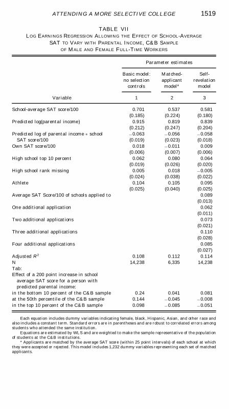
TABLE VIILOG EARNINGS REGRESSION ALLOWING THE EFFECT OF SCHOOL-AVERAGE

SAT TO VARY WITH PARENTAL INCOME, C&B SAMPLE

OF MALE AND FEMALE FULL-TIME WORKERS

Variable

Parameter estimates


controls

Matched-applicantmodel*

Self-revelation

model

1 2 3

School-average SAT score/100 0.701 0.537 0.581(0.185) (0.224) (0.180)

Predicted log(parental income) 0.915 0.819 0.839(0.212) (0.247) (0.204)

Predicted log of parental income p schoolSAT score/100

20.063 20.056 20.058(0.019) (0.023) (0.018)

Own SAT score/100 0.018 20.011 0.009(0.006) (0.007) (0.006)

High school top 10 percent 0.062 0.080 0.064(0.019) (0.026) (0.020)

High school rank missing 0.005 0.018 20.005(0.024) (0.038) (0.022)

Athlete 0.104 0.105 0.095(0.025) (0.040) (0.025)

Average SAT Score/100 of schools applied to 0.089(0.013)

One additional application 0.062(0.011)

Two additional applications 0.073(0.021)

Three additional applications 0.110(0.028)

Four additional applications 0.085(0.027)

Adjusted R2 0.108 0.112 0.114N 14,238 6,335 14,238Tab:Effect of a 200 point increase in school

average SAT score for a person withpredicted parental income:

in the bottom 10 percent of the C&B sample 0.24 0.041 0.081at the 50th percentile of the C&B sample 0.144 20.045 20.008in the top 10 percent of the C&B sample 0.098 20.085 20.051

Each equation includes dummy variables indicating female, black, Hispanic, Asian, and other race andalso includes a constant term. Standard errors are in parentheses and are robust to correlated errors amongstudents who attended the same institution.




Thus, something about schools appears to in�uence earnings. Apossible reason for the insigni�cance of school-average SAT in theselection-adjusted models is that the average SAT score is a crudemeasure of the quality of one’s peer group. Since, to some extent,all schools enroll a heterogeneous group of students, it is possiblefor students to seek out the type of peer group they desire if theyhad attended any of the schools that admitted them. An ablestudent who attends a lower tier school can �nd able students tostudy with, and, alas, a weak student who attends an elite schoolcan �nd other weak students to not study with. What character-istics of schools matter, if not selectivity?

Table VIII presents models in which the logarithm of collegetuition costs net of average student aid is the school qualityindicator.19 These models indicate that students who attendhigher tuition schools earn more after entering the labor market.Notice also that the coef�cient on the interaction term for paren-tal income and tuition (shown in columns 2, 4, and 6) is negative,indicating that there is a higher payoff to attending a moreexpensive school for children from low-income families. The mag-nitude of the coef�cient on tuition falls in the models that adjustfor school selection, but remains sizable.20 For example, the co-ef�cient of .058 in column 5 implies an internal real rate of returnof approximately 15 percent for a person who begins work afterattending college for four years, then earns mean 1995 incomethroughout his career, and retires 44 years later.21 The coef�cientin column 3 implies an internal real rate of return of 13 percent.A caveat to this result, however, is that students who attendhigher cost schools may have higher family wealth (despite ourattempt to control for family income), so tuition may in part pickup the effect of family background on earnings.

Although the implied internal rates of return to investing ina more expensive college in Table VIII are high, one should

19. Net tuition for 1970 and 1980 was calculated by subtracting the averageaid awarded to undergraduates from the sticker price tuition, as reported in theeleventh and twelfth editions of American Universities and Colleges. Then the1976 net tuition was interpolated from the 1970 and 1980 net tuition, assumingan exponential rate of growth.

20. If we control for both net tuition and school SAT score in the sameregression, the effect of net tuition is even larger. For example, the coef�cient(standard error) on tuition from the matched-applicant model is .096 (.017);however, the coef�cient on school SAT score from this model is negative andsigni�cant.

21. This rate of return would fall to 13 percent if we assumed that the personspent 1.5 years in graduate school (the average time spent in graduate school forthe C&B sample) immediately after college.


TABLE VIIILOG EARNINGS REGRESSIONS USING NET TUITION AS SCHOOL QUALITY INDICATOR,

C&B MALE AND FEMALE FULL-TIME WORKERS

Variable

Parameter estimates

Basic models:no selection

controls

Matched-applicantmodels*

Self-revelation

models

1 2 3 4 5 6

Log(net tuition) 0.125 0.711 0.052 0.877 0.058 0.727(0.021) (0.288) (0.022) (0.390) (0.018) (0.283)

Predicted log(parental income) 0.175 0.626 0.159 0.800 0.156 0.671(0.024) (0.215) (0.032) (0.300) (0.024) (0.219)

Log(net tuition) p predicted log(parental income)

20.059 20.083 20.067(0.029) (0.040) (0.029)

Own SAT score/100 0.022 0.022 20.012 20.012 0.009 0.008(0.006) (0.006) (0.007) (0.007) (0.006) (0.006)

Female 20.396 20.395 20.396 20.395 20.396 20.395(0.012) (0.012) (0.024) (0.023) (0.013) (0.013)

Black 20.005 20.005 20.060 20.062 20.039 20.040(0.031) (0.031) (0.052) (0.052) (0.034) (0.035)

Hispanic 0.017 0.011 0.012 0.007 20.006 20.013(0.050) (0.050) (0.100) (0.101) (0.052) (0.053)

Asian 0.178 0.176 0.237 0.236 0.152 0.149(0.033) (0.033) (0.064) (0.064) (0.036) (0.036)

Other/missing race 20.171 20.171 0.067 0.058 20.188 20.188(0.120) (0.120) (0.180) (0.179) (0.117) (0.117)

High school top 10 percent 0.073 0.074 0.083 0.084 0.067 0.067(0.021) (0.021) (0.026) (0.026) (0.021) (0.021)

High school rank missing 0.008 0.009 0.020 0.022 20.006 20.004(0.023) (0.023) (0.039) (0.039) (0.022) (0.022)

Athlete 0.106 0.107 0.102 0.101 0.090 0.091(0.027) (0.027) (0.040) (0.040) (0.024) (0.024)


0.067 0.068(0.012) (0.012)

One additional application 0.052 0.051(0.009) (0.009)

Two additional applications 0.057 0.057(0.019) (0.018)

Three additional applications 0.095 0.095(0.024) (0.024)

Four additional applications 0.071 0.072(0.027) (0.027)

Adjusted R2 0.110 0.110 0.112 0.112 0.115 0.115N 14,238 14,238 6,335 6,335 14,238 14,238

Each equation also includes a constant term. Standard errors are in parentheses, and are robust tocorrelated errors among students who attended the same institution.

Equations are estimated by WLS, and are weighted to make the sample representative of the populationof students at the C&B institutions. Net tuition is average tuition minus average aid (see text).



recognize that the average cost of tuition has roughly doubled inreal terms since the late 1970s, and the payoff to educationincreased in general since the late 1970s. The implicit internalreal rate of return for the estimate in column 5 of Table VIII fallsto 8 percent if tuition costs are doubled. Indeed, the supernormalreturn to investing in high-tuition education in the 1970s mayexplain why it was possible for colleges to raise tuition so much inthe 1980s and 1990s.

College tuition may have a signi�cant effect on subsequentearnings because schools with higher tuition provide their stu-dents with more, or higher quality, resources. We next summa-rize estimates of the effect of expenditures per student on subse-quent earnings. Interestingly, the correlation between tuitionand total expenditures per student in our sample of schools is lessthan .30, so differences in tuition result from factors in addition tospending per student, such as the value of the school’s endow-ment and public support. One should also recognize limitations ofour measures of expenditures per students: (1) undergraduateand graduate student expenditures are combined; (2) there areinherent dif�culties classifying instructional and noninstruc-tional spending; and (3) expenditures are lumpy over time.

To directly explore the effect of school spending, we includedeither the log of total expenditures per student (undergraduateand graduate), or the log of instructional expenditures per stu-dent, in place of tuition in the earnings equation.22 Both mea-sures of expenditures per pupil had a statistically signi�cant andlarge impact on earnings in the basic model. When we estimatedthe matched-applicant model and the self-revelation model, theeffect of expenditures per pupil was smaller and less preciselyestimated. Although the effect of expenditures per pupil wasstatistically insigni�cant, the coef�cient was positive in all butone of the models and implied substantial internal rates of returnto school spending, similar in magnitude to those for tuition.23

These results provide mixed evidence on the effect of expendi-tures per student on students’ subsequent income, perhaps be-cause spending per student is poorly measured.

22. We use 1976 expenditure data from the Integrated Postsecondary Edu-cation Data System (IPEDS) Survey.

23. The coef�cient (and standard error) on log instructional expenditures perstudent if this variable was included instead of tuition in column 1, 3, and 5 ofTable VIII were .114 (.057); .086 (.084); and .024 (.057). The correspondingcoef�cients for log total expenditures per student were .102 (.067); 2.004 (.077);and .008 (.067).


IV. CONCLUSION

The colleges that students attend are affected by selectionon the part of the schools that students apply to, and by selec-tion on the part of the students and their families from themenu of feasible options. A major concern with past estimatesof the payoff to attending an elite college is that more selec-tive schools tend to accept students with higher earnings ca-pacity. This paper adjusts for selection on the part of schoolsby comparing earnings and other outcomes among studentswho applied to, and were accepted and rejected by, a comparableset of institutions. Although our selection correction has manydesirable features, a complete analysis of school selection alsowould model students’ choice of colleges. Nonetheless, since col-lege admission decisions are made by professional administratorswho have much more information at their disposal than research-ers who later analyze student outcomes, we suspect that ourselection correction addresses a major cause of bias in past wageequations.

After we adjust for students’ unobserved characteristics,our �ndings lead us to question the view that school selectivity,as measured by the average SAT score of the freshmen whoattend a college, is an important determinant of students’ sub-sequent incomes. Students who attended more selective col-leges do not earn more than other students who were ac-cepted and rejected by comparable schools but attended lessselective colleges. Additional evidence of omitted variable biasdue to the college application and admissions process comesfrom the fact that the average SAT score of schools that astudent applied to but was rejected from has a stronger ef-fect on the student’s subsequent earnings than the averageSAT score of the school the student actually attended. Fur-thermore, we �nd that students with higher SAT scores aremore likely to attend the most selective college from their set ofoptions, suggesting that students who attend the more selectiveschools may have higher unobserved ability. These results areconsistent with the conclusion of Hunt’s [1963, p. 56] seminalresearch: “The C student from Princeton earns more than the Astudent from Podunk not mainly because he has the prestige of aPrinceton degree, but merely because he is abler. The goldentouch is possessed not by the Ivy League College, but by itsstudents.”


It is possible, however, that attending a highly selectiveschool helps some students and hurts others. If this were the case,and students were aware of it, then the students who chose toattend a less selective school even though they were admitted toa more selective one might be the students with attributes thatlead them to bene�t more from attending a less selective school.If this type of matching is important, then it is important forfamilies to consider the �t between the particular attributes oftheir children and the school they attend. Moreover, if matchingbetween the student’s matriculation decisions and the potentialpayoff for that student from attending a particular (selective)college does take place, our estimates should not be interpreted ascausal. But our results would still suggest that there is not a“one-size-�ts-all” ranking of schools, in which students are al-ways better off in terms of their expected future earnings byattending the most selective school that admits them.

This sentiment was expressed clearly by Stephen R. Lewis,Jr., president of Carleton College, who responded to the U.S.News & World Report college rankings (which ranked his schoolsixth among liberal arts colleges) by saying, “The question shouldnot be, what are the best colleges? The real question should be,best for whom?”24

We do �nd that students who attend colleges with higheraverage tuition costs tend to earn higher income years later, afteradjusting for student characteristics. This �nding is not surpris-ing given that one would expect students to receive a pecuniary ornonpecuniary bene�t from higher tuition costs. Moreover, our�ndings for expenditures per student closely match those fortuition, although the effect of expenditures is less precisely mea-sured. Because tuition and expenditures per student are posi-tively correlated, these results suggest that tuition matters be-cause higher cost schools devote more resources to studentinstruction. The internal real rate of return on college tuition forstudents who attended college in the late 1970s was high, in theneighborhood of 13 to 15 percent. But college tuition costs haverisen considerably since the 1970s, driving the internal rate ofreturn to a more normal level.

Finally, we �nd that the returns to school characteristics suchas average SAT score or tuition are greatest for students from more

24. Quoted in Alex Kuczynski, “ ‘Best’ List For Colleges By U. S. News IsUnder Fire,” The New York Times, August 20, 2001, p. C1.


disadvantaged backgrounds. School admissions and �nancial aidpolicies that have as a goal attracting quali�ed students from moredisadvantaged family backgrounds may raise national income, asthese students appear to bene�t most from attending a more elitecollege. Ellwood and Kane’s [1998] recent �nding that college enroll-ment hardly increased for children from low-income families in the1980s is troubling in this regard.

APPENDIX 1: SCHOOL-AVERAGE SAT SCORE AND NET TUITION OF C&B INSTITUTIONS

InstitutionSchool-average

SAT score in 19781976

Net tuition ($)

Barnard College 1210 3530Bryn Mawr College 1370 3171Columbia University 1330 3591Denison University 1020 3254Duke University 1226 3052Emory University 1150 3237Georgetown University 1225 3304Hamilton College 1246 3529Kenyon College 1155 3329Miami University (Ohio) 1073 1304Northwestern University 1240 3676Oberlin College 1227 3441Pennsylvania State University 1038 1062Princeton University 1308 3613Rice University 1316 1753Smith College 1210 3539Stanford University 1270 3658Swarthmore College 1340 3122Tufts University 1200 3853Tulane University 1080 3269University of Michigan (Ann Arbor) 1110 1517University of North Carolina (Chapel Hill) 1080 541University of Notre Dame 1200 3216University of Pennsylvania 1280 3266Vanderbilt University 1162 3155Washington University 1180 3245Wellesley College 1220 3312Wesleyan University 1260 3368Williams College 1255 3541Yale University 1360 3744

The school-average SAT scores were obtained from HERI, and pertain to freshmen. Net tuition for 1970and 1980 was calculated by subtracting the average aid awarded to undergraduates from the sticker pricetuition, as reported in the eleventh and twelfth editions of American Universities and Colleges. The 1976 nettuition was interpolated from the 1970 and 1980 net tuition, assuming an exponential rate of growth.

MATHEMATICA POLICY RESEARCH, INC

PRINCETON UNIVERSITY


REFERENCES

American Council on Education, American Universities and Colleges, 12th edition(Hawthorn, NY: Walter de Gruyter, 1983).

Barron’s, Barron’s Pro�les of American Colleges (Great Neck, NY: Barron’s Edu-cational Series, 1978).

Barnow, Burt S., Glen G. Cain, and Arthur Goldberger, “Selection on Observ-ables,” Evaluation Studies Review Annual, V (1981), 43–59.

Behrman, Jere R., Jill Constantine, Lori Kletzer, Michael McPherson, and MortonO. Schapiro, “The Impact of College Quality on Wages: Are There Differencesamong Demographic Groups?” Working Paper No. DP-38, William College,1996.

Behrman, Jere R., Mark R. Rosenzweig, and Paul Taubman, “College Choice andWages: Estimates Using Data on Female Twins,” Review of Economics andStatistics, LXXVII (1996), 672–685.

Bowen, William G., and Derek Bok, The Shape of the River: Long-Term Conse-quences of Considering Race in College and University Admissions (Princeton,NJ: Princeton University Press, 1998).

Braun, Henry, and Ted Szatrowski, “The Scale-Linkage Algorithm: Constructionof a Universal Criterion Scale for Families of Institutions,” Journal of Edu-cational Statistics, IX (1984), 311–330.

Breneman, David W., Liberal Arts Colleges: Thriving, Surviving or Endangered?(Washington, DC: The Brookings Institution, 1994).

Brewer, Dominic, and Ronald Ehrenberg, “Does it Pay to Attend an Elite PrivateCollege? Evidence from the Senior High School Class of 1980,” Research inLabor Economics, XV (1996), 239 –271.

Brewer, Dominic, Eric Eide, and Ronald Ehrenberg, “Does it Pay to Attend anElite College? Cross Cohort Evidence on the Effects of College Type onEarnings,” Journal of Human Resources, XXXIV (Winter 1999), 104 –123.

Dale, Stacy Berg, and Alan B. Krueger, “Estimating the Payoff to Attending aMore Selective College: An Application of Selection on Observables and Un-observables,” NBER Working Paper No. W7322, August 1999.

Daniel, Kermit, Dan Black, and Jeffrey Smith, “College Quality and the Wages ofYoung Men,” Research Report No. 9707, Department of Economics, Univer-sity of Western Ontario, 1997.

Ellwood, David, and Thomas Kane, “Who Is Getting a College Education: FamilyBackground and the Growing Gaps in Enrollment,” mimeo, Kennedy Schoolof Government, Harvard University, September 1998.

Furniss, Todd W., ed., American Universities and Colleges, 11th edition (Wash-ington, DC: American Council on Education, 1973).

Griliches, Zvi, “Sibling Models and Data in Economics: Beginnings of a Survey,”Journal of Political Economy, LXXVII (1979), S37–S64.

——, “Economic Data Issues,” in Zvi Griliches and Michael D. Intriligator, eds.,Handbook of Econometrics (Amsterdam: North-Holland, 1986).

Grover, Ronald, “How Steven Spielberg Sustains His Creative Empire,” BusinessWeek, July 13, 1998, 96.

Heckman, James, “Sample Selection Bias as a Speci�cation Error,” Econometrica,XLVII (1979), 153–161.

Hunt, Shane, “Income Determinants for College Graduates and the Return toEducational Investment,” Ph.D. thesis, Yale University, 1963.

Kane, Thomas, “Racial and Ethnic Preferences in College Admission,” in C.Jencks and M. Phillips, eds., The Black-White Test Score Gap (Washington,DC: The Brookings Institution, 1998).

National Association for College Admission Counseling, “Survey ExaminesTrends,” NACAC Bulletin, November, 1998, 1.

Solmon, Lewis, “The De�nition of College Quality,” in Lewis Solmon and PaulTaubman, eds., Does College Matter: Some Evidence on the Impacts of HigherEducation (New York: Academic Press, 1973).

Solmon, Lewis, and Paul Wachtel, “The Effects on Income of Type of CollegeAttended,” Sociology of Education, XLVIII (1975), 75–90.

U. S. Department of Education, National Center for Education Statistics, Digestof Education Statistics 1997, NCES 98-015, Washington, DC: 1997.


Van der Klaauw, Wilbert, “A Regression-Discontinuity Evaluation of the Effect ofFinancial Aid Offers on College Enrollment,” mimeo, Department of Econom-ics, New York University, October 1997.

Wales, Terence, “The Effect of College Quality on Earnings: Results from theNBER-Thorndike Data,” Journal of Human Resources, VIII (1973), 306–317.

Wise, David, “Academic Achievement and Job Performance,” American EconomicReview, LXV, (1975), 350 –366.


estimatingthepayofftoattendingamore …e.g.,studentsat),andanothersetofvariablesthatis...

Documents