estimation frameworks in econometrics...

Greene-2140242 book December 10, 2010 7:46

12

ESTIMATION FRAMEWORKSIN ECONOMETRICS

Q

12.1 INTRODUCTION

This chapter begins our treatment of methods of estimation. Contemporary economet-rics offers the practitioner a remarkable variety of estimation methods, ranging fromtightly parameterized likelihood-based techniques at one end to thinly stated nonpara-metric methods that assume little more than mere association between variables atthe other, and a rich variety in between. Even the experienced researcher could beforgiven for wondering how they should choose from this long menu. It is certainlybeyond our scope to answer this question here, but a few principles can be suggested.Recent research has leaned when possible toward methods that require few (or fewer)possibly unwarranted or improper assumptions. This explains the ascendance of theGMM estimator in situations where strong likelihood-based parameterizations can beavoided and robust estimation can be done in the presence of heteroscedasticity andserial correlation. (It is intriguing to observe that this is occurring at a time when ad-vances in computation have helped bring about increased acceptance of very heavilyparameterized Bayesian methods.)

As a general proposition, the progression from full to semi- to non-parametricestimation relaxes strong assumptions, but at the cost of weakening the conclusionsthat can be drawn from the data. As much as anywhere else, this is clear in the anal-ysis of discrete choice models, which provide one of the most active literatures in thefield. (A sampler appears in Chapter 17.) A formal probit or logit model allows estima-tion of probabilities, marginal effects, and a host of ancillary results, but at the cost ofimposing the normal or logistic distribution on the data. Semiparametric and nonpara-metric estimators allow one to relax the restriction but often provide, in return, onlyranges of probabilities, if that, and in many cases, preclude estimation of probabilitiesor useful marginal effects. One does have the virtue of robustness in the conclusions,however. [See, e.g., the symposium in Angrist (2001) for a spirited discussion on thesepoints.]

Estimation properties is another arena in which the different approaches can becompared. Within a class of estimators, one can define “the best” (most efficient) meansof using the data. (See Example 12.2 for an application.) Sometimes comparisonscan be made across classes as well. For example, when they are estimating the sameparameters—this remains to be established—the best parametric estimator will gener-ally outperform the best semiparametric estimator. That is the value of the information,of course. The other side of the comparison, however, is that the semiparametric esti-mator will carry the day if the parametric model is misspecified in a fashion to whichthe semiparametric estimator is robust (and the parametric model is not).

432


CHAPTER 12 ✦ Estimation Frameworks in Econometrics 433

Schools of thought have entered this conversation for a long time. Proponents ofBayesian estimation often took an almost theological viewpoint in their criticism of theirclassical colleagues. [See, for example, Poirier (1995).] Contemporary practitioners areusually more pragmatic than this. Bayesian estimation has gained currency as a set oftechniques that can, in very many cases, provide both elegant and tractable solutionsto problems that have heretofore been out of reach. Thus, for example, the simulation-based estimation advocated in the many papers of Chib and Greenberg (e.g., 1996) haveprovided solutions to a variety of computationally challenging problems.1 Argumentsas to the methodological virtue of one approach or the other have received much lessattention than before.

Chapters 2 through 7 of this book have focused on the classical regression modeland a particular estimator, least squares (linear and nonlinear). In this and the nextfour chapters, we will examine several general estimation strategies that are used in awide variety of situations. This chapter will survey a few methods in the three broadareas we have listed. Chapter 13 discusses the generalized method of moments, whichhas emerged as the centerpiece of semiparametric estimation. Chapter 14 presents themethod of maximum likelihood, the broad platform for parametric, classical estimationin econometrics. Chapter 15 discusses simulation-based estimation and bootstrapping.This is a recently developed body of techniques that have been made feasible by ad-vances in estimation technology and which has made quite straightforward many es-timators that were previously only scarcely used because of the sheer difficulty of thecomputations. Finally, Chapter 16 introduces the methods of Bayesian econometrics.

The list of techniques presented here is far from complete. We have chosen a setthat constitutes the mainstream of econometrics. Certainly there are others that mightbe considered. [See, for example, Mittelhammer, Judge, and Miller (2000) for a lengthycatalog.] Virtually all of them are the subject of excellent monographs on the subject.In this chapter we will present several applications, some from the literature, somehome grown, to demonstrate the range of techniques that are current in econometricpractice. We begin in Section 12.2 with parametric approaches, primarily maximumlikelihood. Because this is the subject of much of the remainder of this book, thissection is brief. Section 12.2 also introduces Bayesian estimation, which in its traditionalform, is as heavily parameterized as maximum likelihood estimation. Section 12.3 is onsemiparametric estimation. GMM estimation is the subject of all of Chapter 13, so it isonly introduced here. The technique of least absolute deviations is presented here aswell. A range of applications from the recent literature is also surveyed. Section 12.4describes nonparametric estimation. The fundamental tool, the kernel density estimatoris developed, then applied to a problem in regression analysis. Two applications arepresented here as well. Being focused on application, this chapter will say very littleabout the statistical theory for these techniques—such as their asymptotic properties.

1The penetration of Bayesian econometrics could be overstated. It is fairly well represented in current journalssuch as the Journal of Econometrics, Journal of Applied Econometrics, Journal of Business and EconomicStatistics, and so on. On the other hand, in the six major general treatments of econometrics published in 2000,four (Hayashi, Ruud, Patterson, Davidson) do not mention Bayesian methods at all, a buffet of 32 essays(Baltagi) devotes only one to the subject, and the one that displays any preference (Mittelhammer et al.)devotes nearly 10 percent (70) of its pages to Bayesian estimation, but all to the broad metatheory of thelinear regression model and none to the more elaborate applications that form the received applications inthe many journals in the field.


434 PART III ✦ Estimation Methodology

(The results are developed at length in the literature, of course.) We will turn to thesubject of the properties of estimators briefly at the end of the chapter, in Section 12.5,then in greater detail in Chapters 13 through 16.

12.2 PARAMETRIC ESTIMATION AND INFERENCE

Parametric estimation departs from a full statement of the density or probability modelthat provides the data generating mechanism for a random variable of interest. For thesorts of applications we have considered thus far, we might say that the joint density ofa scalar random variable, “y” and a random vector, “x” of interest can be specified by

f (y, x) = g(y | x, β) × h(x | θ), (12-1)

with unknown parameters β and θ . To continue the application that has occupied ussince Chapter 2, consider the linear regression model with normally distributed distur-bances. The assumption produces a full statement of the conditional density that is thepopulation from which an observation is drawn;

yi | xi ∼ N[x′iβ, σ 2].

All that remains for a full definition of the population is knowledge of the specificvalues taken by the unknown, but fixed parameters. With those in hand, the conditionalprobability distribution for yi is completely defined—mean, variance, probabilities ofcertain events, and so on. (The marginal density for the conditioning variables is usuallynot of particular interest.) Thus, the signature features of this modeling platform arespecifications of both the density and the features (parameters) of that density.

The parameter space for the parametric model is the set of allowable values ofthe parameters that satisfy some prior specification of the model. For example, in theregression model specified previously, the K regression slopes may take any real value,but the variance must be a positive number. Therefore, the parameter space for thatmodel is [β, σ 2] ∈ R

K×R+. “Estimation” in this context consists of specifying a criterionfor ranking the points in the parameter space, then choosing that point (a point estimate)or a set of points (an interval estimate) that optimizes that criterion, that is, has the bestranking. Thus, for example, we chose linear least squares as one estimation criterionfor the linear model. “Inference” in this setting is a process by which some regionsof the (already specified) parameter space are deemed not to contain the unknownparameters, though, in more practical terms, we typically define a criterion and then,state that, by that criterion, certain regions are unlikely to contain the true parameters.

12.2.1 CLASSICAL LIKELIHOOD-BASED ESTIMATION

The most common (by far) class of parametric estimators used in econometrics is themaximum likelihood estimators. The underlying philosophy of this class of estimatorsis the idea of “sample information.” When the density of a sample of observations iscompletely specified, apart from the unknown parameters, then the joint density ofthose observations (assuming they are independent), is the likelihood function

f (y1, y2, . . . , x1, x2, . . .) =n∏

i=1

f (yi , xi | β, θ). (12-2)



This function contains all the information available in the sample about the populationfrom which those observations were drawn. The strategy by which that information isused in estimation constitutes the estimator.

The maximum likelihood estimator [Fisher (1925)] is the function of the data that(as its name implies) maximizes the likelihood function (or, because it is usually moreconvenient, the log of the likelihood function). The motivation for this approach ismost easily visualized in the setting of a discrete random variable. In this case, thelikelihood function gives the joint probability for the observed sample observations,and the maximum likelihood estimator is the function of the sample information thatmakes the observed data most probable (at least by that criterion). Though the analogyis most intuitively appealing for a discrete variable, it carries over to continuous variablesas well. Since this estimator is the subject of Chapter 14, which is quite lengthy, we willdefer any formal discussion until then and consider instead two applications to illustratethe techniques and underpinnings.

Example 12.1 The Linear Regression ModelLeast squares weighs negative and positive deviations equally and gives disproportionateweight to large deviations in the calculation. This property can be an advantage or a disad-vantage, depending on the data generating process. For normally distributed disturbances,this method is precisely the one needed to use the data most efficiently. If the data aregenerated by a normal distribution, then the log of the likelihood function is

ln L = −n2

ln 2π − n2

ln σ 2 − 12σ 2

(y − Xβ) ′(y − Xβ) .

You can easily show that least squares is the estimator of choice for this model. Maximizingthe function means minimizing the exponent, which is done by least squares for β, then e′e/nfollows as the estimator for σ 2.

If the appropriate distribution is deemed to be something other than normal—perhaps onthe basis of an observation that the tails of the disturbance distribution are too thick—seeExample 4.7 and Section 14.9.5.a—then there are three ways one might proceed. First, as wehave observed, the consistency of least squares is robust to this failure of the specification, solong as the conditional mean of the disturbances is still zero. Some correction to the standarderrors is necessary for proper inferences. Second, one might want to proceed to an estimatorwith better finite sample properties. The least absolute deviations estimator discussed inSection 12.3.2 is a candidate. Finally, one might consider some other distribution whichaccommodates the observed discrepancy. For example, Ruud (2000) examines in somedetail a linear regression model with disturbances distributed according to the t distributionwith v degrees of freedom. As long as v is finite, this random variable will have a largervariance than the normal. Which way should one proceed? The third approach is the leastappealing. Surely if the normal distribution is inappropriate, then it would be difficult to comeup with a plausible mechanism whereby the t distribution would not be. The LAD estimatormight well be preferable if the sample were small. If not, then least squares would probablyremain the estimator of choice, with some allowance for the fact that standard inference toolswould probably be misleading. Current practice is generally to adopt the first strategy.

Example 12.2 The Stochastic Frontier ModelThe stochastic frontier model, discussed in detail in Chapter 19, is a regression-like modelwith a disturbance distribution that is asymmetric and distinctly nonnormal. The conditionaldensity for the dependent variable in this model is

f ( y | x, β, σ, λ) =√

2σ√

πexp

[−( y − α − x′β) 2

2σ 2

]�

(−λ( y − α − x′β)σ

).



This produces a log-likelihood function for the model,

ln L = −n ln σ − n2

ln2π

− 12

n∑i =1

(εi

σ

)2

+n∑

i =1

ln �

(−λεi

σ

).

There are at least two fully parametric estimators for this model. The maximum likelihoodestimator is discussed in Section 19.2.4. Greene (2007) presents the following method ofmoments estimator: For the regression slopes, excluding the constant term, use leastsquares. For the parameters α, σ , and λ, based on the second and third moments of theleast squares residuals and the least squares constant, solve

m2 = σ 2v + [1 − 2/π ]σ 2

u ,

m3 = (2/π ) 1/2[1 − 4/π ]σ 3u ,

a = α + (2/π ) 2σu,

where λ = σu/σv and σ 2 = σ 2u + σ 2

v .Both estimators are fully parametric. The maximum likelihood estimator is for the reasons

discussed earlier. The method of moments estimators (see Section 13.2) are appropriate onlyfor this distribution. Which is preferable? As we will see in Chapter 19, both estimators areconsistent and asymptotically normally distributed. By virtue of the Cramer–Rao theorem,the maximum likelihood estimator has a smaller asymptotic variance. Neither has any smallsample optimality properties. Thus, the only virtue of the method of moments estimator isthat one can compute it with any standard regression/statistics computer package and ahand calculator whereas the maximum likelihood estimator requires specialized software(only somewhat—it is reasonably common).

12.2.2 MODELING JOINT DISTRIBUTIONS WITHCOPULA FUNCTIONS

Specifying the likelihood function commits the analyst to a possibly strong assump-tion about the distribution of the random variable of interest. The payoff, of course, isthe stronger inferences that this permits. However, when there is more than one ran-dom variable of interest, such as in a joint household decision on health care usage inthe example to follow, formulating the full likelihood involves specifying the marginaldistributions, which might be comfortable, and a full specification of the joint distri-bution, which is likely to be less so. In the typical situation, the model might involvetwo similar random variables and an ill-formed specification of correlation betweenthem. Implicitly, this case involves specification of the marginal distributions. The jointdistribution is an empirical necessity to allow the correlation to be nonzero. The copulafunction approach provides a mechanism that the researcher can use to steer aroundthis situation.

Trivedi and Zimmer (2007) suggest a variety of applications that fit this description:

• Financial institutions are often concerned with the prices of different, related(dependent) assets. The typical multivariate normality assumption is problematicbecause of GARCH effects (see Section 20.13) and thick tails in the distributions.While specifying appropriate marginal distributions may be reasonably straight-forward, specifying the joint distribution is anything but that. Klugman and Parsa(2000) is an application.

• There are many microeconometric applications in which straightforward marginaldistributions cannot be readily combined into a natural joint distribution. The



bivariate event count model analyzed in Munkin and Trivedi (1999) and in thenext example is an application.

• In the linear self-selection model of Chapter 19, the necessary joint distribution ispart of a larger model. The likelihood function for the observed outcome involvesthe joint distribution of a variable of interest, hours, wages, income, and so on, andthe probability of observation. The typical application is based on a joint normaldistribution. Smith (2003, 2005) suggests some applications in which a flexible cop-ula representation is more appropriate. [In an intriguing early application of copulamodeling that was not labeled as such, since it greatly predates the econometric lit-erature, Lee (1983) modeled the outcome variable in a selectivity model as normal,the observation probability as logistic, and the connection between them using whatamounted to the “Gaussian” copula function shown next.]

Although the antecedents in the statistics literature date to Sklar’s (1973) derivations,the applications in econometrics and finance are quite recent, with most applicationsappearing since 2000. [See the excellent survey by Trivedi and Zimmer (2007) for anextensive description.]

Consider a modeling problem in which the marginal cdfs of two random variablescan be fully specified as F1(y1 | •) and F2(y2 | •), where we condition on sample infor-mation (data) and parameters denoted “•.” For the moment, assume these are con-tinuous random variables that obey all the axioms of probability. The bivariate cdf isF12(y1, y2 | •). A (bivariate) copula function (the results also extend to multivariate func-tions) is a function C(u1, u2) defined over the unit square [(0 ≤ u1 ≤ 1) × (0 ≤ u2 ≤ 1)]that satisfies

(1) C(1, u2) = u2 and C(u1, 1) = u1,

(2) C(0, u2) = C(u1, 0) = 0,

(3) ∂C(u1, u2)/∂u1 ≥ 0 and ∂C(u1, u2)/∂u2 ≥ 0.

These are properties of bivariate cdfs for random variables u1 and u2 that are boundedin the unit square. It follows that the copula function is a two-dimensional cdf definedover the unit square that has one-dimensional marginal distributions that are standarduniform in the unit interval [that is, property (1)]. To make profitable use of this re-lationship, we note that the cdf of a random variable, F1(y1 | •), is, itself, a uniformlydistributed random variable. This is the fundamental probability transform that weuse for generating random numbers. (See Section 15.2.) In Sklar’s (1973) theorem, themarginal cdfs play the roles of u1 and u2. The theorem states that there exists a copulafunction, C(. , .) such that

F12(y1, y2 | •) = C[F1(y1 | •), F2(y2 | •)].

If F12(y1, y2 | •) = C[F1(y1 | •), F2(y2 | •)] is continuous and if the marginal cdfs havequantile (inverse) functions F−1

j (u j ) where 0 ≤ u j ≤ 1, then the copula function canbe expressed as

F12(y1, y2 | •) = F12[F−1

1 (u1 | •), F−12 (u2 | •)

]= Prob[U1 ≤ u1, U2 ≤ u2]

= C(u1, u2).



In words, the theorem implies that the joint density can be written as the copula functionevaluated at the two cumulative probability functions.

Copula functions allow the analyst to assemble joint distributions when only themarginal distributions can be specified. To fill in the desired element of correlationbetween the random variables, the copula function is written

F12(y1, y2 | •) = C[F1(y1 | •), F2(y2 | •), θ ],

where θ is a “dependence parameter.” For continuous random variables, the joint pdfis then the mixed partial derivative,

f12(y1, y2 | •) = c12[F1(y1 | •), F2(y2 | •), θ ]

= ∂2C[F1(y1 | •), F2(y2 | •), θ ]/∂y1∂y2 (12-3)

= [∂2C(., ., θ)/∂ F1∂ F2] f1(y1 | •) f2(y2 | •).

A log-likelihood function can now be constructed using the logs of the right-hand sides of(12-3). Taking logs of (12-3) reveals the utility of the copula approach. The contributionof the joint observation to the log likelihood is

ln f12(y1, y2 | •) = ln[∂2C(., ., θ)/∂ F1∂ F2] + ln f1(y1 | •) + ln f2(y2 | •).

Some of the common copula functions that have been used in applications are as follows:

Product: C[u1, u2, θ ] = u1 × u2,

FGM: C[u1, u2, θ ] = u1u2[1 + θ(1 − u1)(1 − u2)],

Gaussian: C[u1, u2, θ ] = �2[�−1(u1), �−1(u2), θ ],

Clayton: C[u1, u2, θ ] = [u−θ

1 + u−θ2 − 1

]−1/θ,

Frank: C[u1, u2, θ ] = 1θ

ln[

1 + exp(θu1 − 1)exp(θu2 − 1)

exp(θ) − 1

].

The product copula implies that the random variables are independent, because it im-plies that the joint cdf is the product of the marginals. In the FGM (Fairlie, Gumbel,Morgenstern) copula, it can be seen that θ = 0 implies the product copula, or indepen-dence. The same result can be shown for the Clayton copula. In the Gaussian function,the copula is the bivariate normal cdf if the marginals happen to be normal to beginwith. The essential point is that the marginals need not be normal to construct the copulafunction, so long as the marginal cdfs can be specified. (The dependence parameter isnot the correlation between the variables. Trivedi and Zimmer provide transformationsof θ that are closely related to correlations for each copula function listed.)

The essence of the copula technique is that the researcher can specify and analyzethe marginals and the copula functions separately. The likelihood function is obtainedby formulating the cdfs [or the densities, because the differentiation in (12-3) will reducethe joint density to a convenient function of the marginal densities] and the copula.

Example 12.3 Joint Modeling of a Pair of Event CountsThe standard regression modeling approach for a random variable, y, that is a count of eventsis the Poisson regression model,

Prob[Y = y | x] = exp(−λ)λy/y!, where λ = exp(x′β) , y = 0, 1, . . . .



More intricate specifications use the negative binomial model (version 2, NB2),

Prob[Y = y | x] = ( y + α)(α)( y + 1)

(α

λ + α

)α(

λ

λ + α

)y

, y = 0, 1, . . . ,

where α is an overdispersion parameter. (See Section 18.4.) A satisfactory, appropriate speci-fication for bivariate outcomes has been an ongoing topic of research. Early suggestions werebased on a latent mixture model,

y1 = z + w1,

y2 = z + w2,

where w1 and w2 have the Poisson or NB2 distributions specified earlier with conditionalmeans λ1 and λ2 and z is taken to be an unobserved Poisson or NB variable. This formulationinduces correlation between the variables but is unsatisfactory because that correlation mustbe positive. In a natural application, y1 is doctor visits and y2 is hospital visits. These couldbe negatively correlated. Munkin and Trivedi (1999) specified the jointness in the conditionalmean functions, in the form of latent, common heterogeneity;

λ j = exp(x′j β j + ε)

where ε is common to the two functions. Cameron et al. (2004) used a bivariate copulaapproach to analyze Australian data on self-reported and actual physician visits (the lat-ter maintained by the Health Insurance Commission). They made two adjustments to thepreceding model we developed above. First, they adapted the basic copula formulation tothese discrete random variables. Second, the variable of interest to them was not the actualor self-reported count, but the difference. Both of these are straightforward modifications ofthe basic copula model.

12.3 SEMIPARAMETRIC ESTIMATION

Semiparametric estimation is based on fewer assumptions than parametric estimation.In general, the distributional assumption is removed, and an estimator is devised fromcertain more general characteristics of the population. Intuition suggests two (correct)conclusions. First, the semiparametric estimator will be more robust than the parametricestimator—it will retain its properties, notably consistency across a greater range ofspecifications. Consider our most familiar example. The least squares slope estimator isconsistent whenever the data are well behaved and the disturbances and the regressorsare uncorrelated. This is even true for the frontier function in Example 12.2, which hasan asymmetric, nonnormal disturbance. But, second, this robustness comes at a cost.The distributional assumption usually makes the preferred estimator more efficientthan a robust one. The best robust estimator in its class will usually be inferior to theparametric estimator when the assumption of the distribution is correct. Once again,in the frontier function setting, least squares may be robust for the slopes, and it isthe most efficient estimator that uses only the orthogonality of the disturbances andthe regressors, but it will be inferior to the maximum likelihood estimator when thetwo-part normal distribution is the correct assumption.

12.3.1 GMM ESTIMATION IN ECONOMETRICS

Recent applications in economics include many that base estimation on the methodof moments. The generalized method of moments departs from a set of model based



moment equations, E [m(yi , xi , β)] = 0, where the set of equations specifies a relation-ship known to hold in the population. We used one of these in the preceding paragraph.The least squares estimator can be motivated by noting that the essential assumption isthat E [xi (yi − x′

iβ)] = 0. The estimator is obtained by seeking a parameter estimator,b, which mimics the population result; (1/n)�i [xi (yi − x′

i b)] = 0. These are, of course,the normal equations for least squares. Note that the estimator is specified without ben-efit of any distributional assumption. Method of moments estimation is the subject ofChapter 13, so we will defer further analysis until then.

12.3.2 MAXIMUM EMPIRICAL LIKELIHOOD ESTIMATION

Empirical likelihood methods are suggested as a semiparametric alternative to maxi-mum likelihood. As we shall see shortly, the estimator is closely related to the GMMestimator. Let πi denote generically the probability that yi |xi takes the realized value inthe sample. Intuition suggests (correctly) that with no further information, πi will equal1/n. The empirical likelihood function is

EL =∏n

i=1π

1/ni .

The maximum empirical likelihood estimator maximizes EL. Equivalently, we maximizethe log of the empirical likelihood,

ELL = 1n

n∑i=1

ln πi .

As a maximization problem, this program lacks sufficient structure to admit a solution—the solutions for πi are unbounded. If we impose the restrictions that πi are probabilitiesthat sum to one, we can use a Langragean formulation to solve the optimization problem,

ELL =[

1n

n∑i=1

ln πi

]+ λ

[1 −

n∑i=1

πi

].

This slightly restricts the problem since with 0 < πi < 1 and �iπi = 1, the solutionsuggested earlier becomes obvious. (There is nothing in the problem that differentiatesthe πi ’s, so they must all be equal to each other.) Inserting this result in the derivativewith respect to any specific πi produces the remaining result, λ = 1.

The maximization problem becomes meaningful when we impose a structure on thedata. To develop an example, we’ll recall Example 7.6, a nonlinear regression equationfor Income for the German Socioeconomic Panel data, where we specified

E[Income|Age, Sex, Education] = exp(x′β) = h(x, β).

For purpose of an example, assume that Education may be endogenous in this equation,but we have available a set of instruments, z, say (Age, Health, Sex, MarketCondition).We have assumed that there are more instruments (4) than included variables (3), so thatthe parameters will be overidentified (and the example will be complicated enough tobe interesting). (See Sections 8.3.4 and 8.6.) The orthogonality conditions for nonlinearinstrumental variable estimation are that the disturbances be uncorrelated with theinstrumental variables, so

E{zi [Incomei − h(xi , β)]} = E[mi (β)] = 0.



The nonlinear least squares solution to this problem was developed in Section 8.6. AGMM estimator will minimize with respect to β the criterion function

q = m′(β)Am(β)

where A is the chosen weighting matrix. Note that for our example, including the con-stant term, there are four elements in β and five moment equations, so the parametersare overidentified.

If we impose the restrictions implied by our moment equations on the empiricallikelihood function, instead, we obtain the population moment condition[

n∑i=1

πi zi (Incomei − h(xi , β))

]= 0.

(The probabilities are population quantities, so this is the expected value.) This producesthe constrained empirical log likelihood

ELL =[

1n

n∑i=1

ln πi

]+ λ

[1 −

n∑i=1

πi

]+ γ ′

[n∑

i=1

πi zi (Incomei − h(xi , β))

].

The function is now maximized with respect to πi , λ, β (K elements) and γ (L ele-ments, the number of instrumental variables). At the solution, the values of πi provide,essentially, a set of weights. Cameron and Trivedi (2005, p. 205) provide a solution forπi in terms of (β, γ ) and show, once again, that λ = 1. The concentrated ELL functionwith these inserted provides a function of γ and β that remains to be maximized.

The empirical likelihood estimator has the same asymptotic properties as theGMM estimator. (This makes sense, given the resemblance of the estimation criteria—ultimately, both are focused on the moment equations.) There is evidence that at least insome cases, the finite sample properties of the empirical likelihood estimator might bebetter than GMM. A survey appears in Imbens (2002). One suggested modification ofthe procedure is to replace the core function in (1/n)�i ln πi with the entropy measure,

Entropy = (1/n)�iπi ln πi .

The maximum entropy estimator is developed in Golan, Judge, and Miller (1996) andGolan (2009).

12.3.3 LEAST ABSOLUTE DEVIATIONS ESTIMATIONAND QUANTILE REGRESSION

Least squares can be severely distorted by outlying observations in a small sample.Recent applications in microeconomics and financial economics involving thick-taileddisturbance distributions, for example, are particularly likely to be affected by preciselythese sorts of observations. (Of course, in those applications in finance involving hun-dreds of thousands of observations, which are becoming commonplace, this discussionis moot.) These applications have led to the proposal of “robust” estimators that areunaffected by outlying observations. One of these, the least absolute deviations, or LADestimator discussed in Section 7.3.1, is also useful in its own right as an estimator of theconditional median function in the modified model

Med[y|x] = x′β .50.



That is, rather than providing a robust alternative to least squares as an estimator ofthe slopes of E[y|x], LAD is an estimator of a different feature of the population. Thisis essentially a semiparametric specification in that it specifies only a particular featureof the distribution, its median, but not the distribution itself. It also specifies that theconditional median be a linear function of x.

The median, in turn, is only one possible quantile of interest. If the model is extendedto other quantiles of the conditional distribution, we obtain

Q[y|x, q] = x′βq such that Prob[y < x′βq|x] = q, 0 < q < 1.

This is essentially a nonparametric specification. No assumption is made about the dis-tribution of y|x or about its conditional variance. The fact that q can vary continuously(strictly) between zero and one means that there is an infinite number of possible “pa-rameter vectors.” It seems reasonable to view the coefficients, which we might writeβ(q) less as fixed “parameters,” as we do in the linear regression model, than looselyas features of the distribution of y|x. For example, it is not likely to be meaningfulto view β(.49) to be discretely different from β(.50) or to compute precisely a partic-ular difference such as β(.5) − β(.3). On the other hand, the qualitative difference,or possibly the lack of a difference, between β(.3) and β(.5) may well be an inter-esting characteristic of the population. The quantile regression model is examined inSection 7.3.2.

12.3.4 KERNEL DENSITY METHODS

The kernel density estimator is an inherently nonparametric tool, so it fits more ap-propriately into the next section. But some models that use kernel methods are notcompletely nonparametric. The partially linear model in Section 7.4 is a case in point.Many models retain an index function formulation, that is, build the specification arounda linear function, x′β, which makes them at least semiparametric, but nonetheless stillavoid distributional assumptions by using kernel methods. Lewbel’s (2000) estimatorfor the binary choice model is another example.

Example 12.4 Semiparametric Estimator for Binary Choice ModelsThe core binary choice model analyzed in Section 17.3, the probit model, is a fully parametricspecification. Under the assumptions of the model, maximum likelihood is the efficient (andappropriate) estimator. However, as documented in a voluminous literature, the estimator ofβ is fragile with respect to failures of the distributional assumption. We will examine a fewsemiparametric and nonparametric estimators in Section 17.4.7. To illustrate the nature ofthe modeling process, we consider an estimator suggested by Lewbel (2000). The probitmodel is based on the normal distribution, with Prob[ yi = 1 | xi ] = Prob[x′

i β + εi > 0] whereεi ∼ N[0, 1]. The estimator of β under this specification will be inconsistent if the distributionis not normal or if εi is heteroscedastic. Lewbel suggests the following: If (a) it can be as-sumed that xi contains a “special” variable, vi , whose coefficient has a known sign–a methodis developed for determining the sign and (b) the density of εi is independent of this vari-able, then a consistent estimator of β can be obtained by regression of [yi − s(vi ) ]/ f (vi | xi )on xi where s(vi ) = 1 if vi > 0 and 0 otherwise and f (vi | xi ) is a kernel density estimatorof the density of vi | xi . Lewbel’s estimator is robust to heteroscedasticity and distribution.A method is also suggested for estimating the distribution of εi . Note that Lewbel’s estimatoris semiparametric. His underlying model is a function of the parameters β, but the distributionis unspecified.



12.3.5 COMPARING PARAMETRIC AND SEMIPARAMETRICANALYSES

It is often of interest to compare the outcomes of parametric and semiparametric mod-els. As we have noted earlier, the strong assumptions of the fully parametric model comeat a cost; the inferences from the model are only as robust as the underlying assump-tions. Of course, the other side of that equation is that when the assumptions are met,parametric models represent efficient strategies for analyzing the data. The alternative,semiparametric approaches relax assumptions such as normality and homoscedasticity.It is important to note that the model extensions to which semiparametric estimatorsare typically robust render the more heavily parameterized estimators inconsistent. Thecomparison is not just one of efficiency. As a consequence, comparison of parameterestimates can be misleading—the parametric and semiparametric estimators are oftenestimating very different quantities.

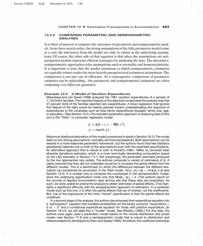
Example 12.5 A Model of Vacation ExpendituresMelenberg and van Soest (1996) analyzed the 1981 vacation expenditures of a sample of1,143 Dutch families. The important feature of the data that complicated the analysis was that37 percent (423) of the families reported zero expenditures. A linear regression that ignoresthis feature of the data would be heavily skewed toward underestimating the response ofexpenditures to the covariates such as total family expenditures (budget), family size, age,or education. (See Section 19.3.) The standard parametric approach to analyzing data of thissort is the “Tobit,” or censored, regression model:

y∗i = x′

i β + εi , εi ∼ N[0, σ 2],

yi = max(0, y∗i ) .

(Maximum likelihood estimation of this model is examined in detail in Section 19.3.) The modelrests on two strong assumptions, normality and homoscedasticity. Both assumptions can berelaxed in a more elaborate parametric framework, but the authors found that test statisticspersistently rejected one or both of the assumptions even with the extended specifications.An alternative approach that is robust to both is Powell’s (1984, 1986a, b) censored leastabsolute deviations estimator, which is a more technically demanding computation basedon the LAD estimator in Section 7.3.1. Not surprisingly, the parameter estimates producedby the two approaches vary widely. The authors computed a variety of estimators of β. Auseful exercise that they did not undertake would be to compare the partial effects from thedifferent models. This is a benchmark on which the differences between the different esti-mators can sometimes be reconciled. In the Tobit model, ∂E [ yi | xi ] /∂xi = �(x′

i β/σ )β (seeSection 19.3). It is unclear how to compute the counterpart in the semiparametric model,since the underlying specification holds only that Med[εi | xi ] = 0. (The authors report onthe Journal of Applied Econometrics data archive site that these data are proprietary. Assuch, we were unable to extend the analysis to obtain estimates of partial effects.) This high-lights a significant difficulty with the semiparametric approach to estimation. In a nonlinearmodel such as this one, it is often the partial effects that are of interest, not the coefficients.But, one of the byproducts of the more “robust” specification is that the partial effects areundefined.

In a second stage of the analysis, the authors decomposed their expenditure equation intoa “participation” equation that modeled probabilities for the binary outcome “expenditure =0 or > 0” and a conditional expenditure equation for those with positive expenditure. [InSection 18.4.8, we will label this a “hurdle” model. See Mullahy (1986).] For this step, theauthors once again used a parametric model based on the normal distribution (the probitmodel—see Section 17.3) and a semiparametric model that is robust to distribution andheteroscedasticity developed by Klein and Spady (1993). As before, the coefficient estimates



1.0

0.0

0.1

0.2

0.3

0.4

0.5

0.6

0.7

0.8

0.9

9.7T

12.412.111.811.511.210.910.610.310.0

Normal Distr.Klein/Spady

FIGURE 12.1 Predicted Probabilities of Positive Expenditure.

differ substantially. However, in this instance, the specification tests are considerably moresympathetic to the parametric model. Figure 12.1, which reproduces their Figure 2, comparesthe predicted probabilities from the two models. The dashed curve is the probit model. Withinthe range of most of the data, the models give quite similar predictions. Once again, however,it is not possible to compare partial effects. The interesting outcome from this part of theanalysis seems to be that the failure of the parametric specification resides more in themodeling of the continuous expenditure variable than with the model that separates the twosubsamples based on zero or positive expenditures.

12.4 NONPARAMETRIC ESTIMATION

Researchers have long held reservations about the strong assumptions made in para-metric models fit by maximum likelihood. The linear regression model with normaldisturbances is a leading example. Splines, translog models, and polynomials all repre-sent attempts to generalize the functional form. Nonetheless, questions remain abouthow much generality can be obtained with such approximations. The techniques of non-parametric estimation discard essentially all fixed assumptions about functional formand distribution. Given their very limited structure, it follows that nonparametric spec-ifications rarely provide very precise inferences. The benefit is that what informationis provided is extremely robust. The centerpiece of this set of techniques is the kerneldensity estimator that we have used in the preceding examples. We will examine someexamples, then examine an application to a bivariate regression.2

2The set of literature in this area of econometrics is large and rapidly growing. Major references whichprovide an applied and theoretical foundation are Hardle (1990), Pagan and Ullah (1999), and Li and Racine(2007).



12.4.1 KERNEL DENSITY ESTIMATION

Sample statistics such as a mean, variance, and range give summary information aboutthe values that a random variable may take. But, they do not suffice to show the distribu-tion of values that the random variable takes, and these may be of interest as well. Thedensity of the variable is used for this purpose. A fully parametric approach to densityestimation begins with an assumption about the form of a distribution. Estimation ofthe density is accomplished by estimation of the parameters of the distribution. To takethe canonical example, if we decide that a variable is generated by a normal distributionwith mean μ and variance σ 2, then the density is fully characterized by these parameters.It follows that

f (x) = f (x | μ, σ 2) = 1σ

1√2π

exp

[−1

2

(x − μ

σ

)2]

.

One may be unwilling to make a narrow distributional assumption about the density.The usual approach in this case is to begin with a histogram as a descriptive device.Consider an example. In Examples 15.17 and in Greene (2004a), we estimate a modelthat produces a conditional estimator of a slope vector for each of the 1,270 firms inour sample. We might be interested in the distribution of these estimators across firms.In particular, the conditional estimates of the estimated slope on ln sales for the 1,270firms have a sample mean of 0.3428, a standard deviation of 0.08919, a minimum of0.2361, and a maximum of 0.5664. This tells us little about the distribution of values,though the fact that the mean is well below the midrange of 0.4013 might suggest someskewness. The histogram in Figure 12.2 is much more revealing. Based on what we see

FIGURE 12.2 Histogram for Estimated bsales Coefficients.

324

243

0.236 0.283 0.330 0.377 0.424bsales

0.471 0.518 0.565

Freq

uenc

y

162

81

0



thus far, an assumption of normality might not be appropriate. The distribution seemsto be bimodal, but certainly no particular functional form seems natural.

The histogram is a crude density estimator. The rectangles in the figure are calledbins. By construction, they are of equal width. (The parameters of the histogram arethe number of bins, the bin width, and the leftmost starting point. Each is importantin the shape of the end result.) Because the frequency count in the bins sums to thesample size, by dividing each by n, we have a density estimator that satisfies an obviousrequirement for a density; it sums (integrates) to one. We can formalize this by layingout the method by which the frequencies are obtained. Let xk be the midpoint of thekth bin and let h be the width of the bin—we will shortly rename h to be the bandwidthfor the density estimator. The distances to the left and right boundaries of the bins areh/2. The frequency count in each bin is the number of observations in the sample whichfall in the range xk ± h/2. Collecting terms, we have our “estimator”

f (x) = 1n

frequency in binx

width of binx= 1

n

n∑i=1

1h

1(

x − h2

< xi < x + h2

),

where 1(statement) denotes an indicator function that equals 1 if the statement is trueand 0 if it is false and binx denotes the bin which has x as its midpoint. We see, then, thatthe histogram is an estimator, at least in some respects, like other estimators we haveencountered. The event in the indicator can be rearranged to produce an equivalentform

f (x) = 1n

n∑i=1

1h

1(

−12

<xi − x

h<

12

).

This form of the estimator simply counts the number of points that are within onehalf-bin width of xk.

Albeit rather crude, this “naive” (its formal name in the literature) estimator is inthe form of kernel density estimators that we have met at various points;

f (x) = 1n

n∑i=1

1h

K[

xi − xh

], where K[z] = 1[−1/2 < z < 1/2].

The naive estimator has several shortcomings. It is neither smooth nor continuous.Its shape is partly determined by where the leftmost and rightmost terminals of thehistogram are set. (In constructing a histogram, one often chooses the bin width to bea specified fraction of the sample range. If so, then the terminals of the lowest andhighest bins will equal the minimum and maximum values in the sample, and this willpartly determine the shape of the histogram. If, instead, the bin width is set irrespectiveof the sample values, then this problem is resolved.) More importantly, the shape ofthe histogram will be crucially dependent on the bandwidth itself. (Unfortunately, thisproblem remains even with more sophisticated specifications.)

The crudeness of the weighting function in the estimator is easy to remedy. Rosen-blatt’s (1956) suggestion was to substitute for the naive estimator some other weightingfunction which is continuous and which also integrates to one. A number of candidateshave been suggested, including the (long) list in Table 12.1. Each of these is smooth,continuous, symmetric, and equally attractive. The logit and normal kernels are definedso that the weight only asymptotically falls to zero whereas the others fall to zero at



TABLE 12.1 Kernels for Density Estimation

Kernel Formula K[z]

Epanechnikov 0.75(1 − 0.2z2)/2.236 if |z| ≤ 5, 0 elseNormal φ(z) (normal density),Logit (z)[1 − (z)] (logistic density)Uniform 0.5 if |z| ≤ 1, 0 elseBeta 0.75(1 − z)(1 + z) if |z| ≤ 1, 0 elseCosine 1 + cos(2πz) if |z| ≤ 0.5, 0 elseTriangle 1 − |z|, if |z| ≤ 1, 0 elseParzen 4/3 − 8z2 + 8 |z|3 if |z| ≤ 0.5, 8(1 − |z|)3/3 if 0.5 < |z| ≤ 1, 0 else.

specific points. It has been observed that in constructing a density estimator, the choiceof kernel function is rarely crucial, and is usually minor in importance compared tothe more difficult problem of choosing the bandwidth. (The logit and normal kernelsappear to be the default choice in many applications.)

The kernel density function is an estimator. For any specific x, f (x) is a samplestatistic,

f (z) = 1n

n∑i=1

g(xi | z, h).

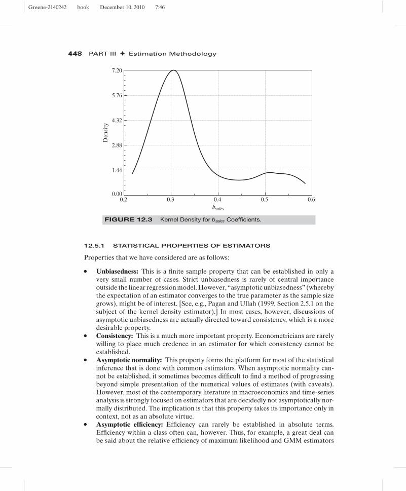
Because g(xi | z, h) is nonlinear, we should expect a bias in a finite sample. It is temptingto apply our usual results for sample moments, but the analysis is more complicatedbecause the bandwidth is a function of n. Pagan and Ullah (1999) have examined theproperties of kernel estimators in detail and found that under certain assumptions,the estimator is consistent and asymptotically normally distributed but biased in finitesamples. The bias is a function of the bandwidth, but for an appropriate choice of h, thebias does vanish asymptotically. As intuition might suggest, the larger is the bandwidth,the greater is the bias, but at the same time, the smaller is the variance. This might suggesta search for an optimal bandwidth. After a lengthy analysis of the subject, however, theauthors’ conclusion provides little guidance for finding one. One consideration doesseem useful. For the proportion of observations captured in the bin to converge to thecorresponding area under the density, the width itself must shrink more slowly than 1/n.Common applications typically use a bandwidth equal to some multiple of n−1/5 for thisreason. Thus, the one we used earlier is h = 0.9 × s/n1/5. To conclude the illustrationbegun earlier, Figure 12.3 is a logit-based kernel density estimator for the distributionof slope estimates for the model estimated earlier. The resemblance to the histogramin Figure 12.2 is to be expected.

12.5 PROPERTIES OF ESTIMATORS

The preceding has been concerned with methods of estimation. We have surveyed avariety of techniques that have appeared in the applied literature. We have not yetexamined the statistical properties of these estimators. Although, as noted earlier, wewill leave extensive analysis of the asymptotic theory for more advanced treatments, itis appropriate to spend at least some time on the fundamental theoretical platform thatunderlies these techniques.



0.20.00

0.3 0.4bsales

Den

sity

0.5 0.6

7.20

5.76

4.32

2.88

1.44

FIGURE 12.3 Kernel Density for bsales Coefficients.

12.5.1 STATISTICAL PROPERTIES OF ESTIMATORS

Properties that we have considered are as follows:

• Unbiasedness: This is a finite sample property that can be established in only avery small number of cases. Strict unbiasedness is rarely of central importanceoutside the linear regression model. However, “asymptotic unbiasedness” (wherebythe expectation of an estimator converges to the true parameter as the sample sizegrows), might be of interest. [See, e.g., Pagan and Ullah (1999, Section 2.5.1 on thesubject of the kernel density estimator).] In most cases, however, discussions ofasymptotic unbiasedness are actually directed toward consistency, which is a moredesirable property.

• Consistency: This is a much more important property. Econometricians are rarelywilling to place much credence in an estimator for which consistency cannot beestablished.

• Asymptotic normality: This property forms the platform for most of the statisticalinference that is done with common estimators. When asymptotic normality can-not be established, it sometimes becomes difficult to find a method of progressingbeyond simple presentation of the numerical values of estimates (with caveats).However, most of the contemporary literature in macroeconomics and time-seriesanalysis is strongly focused on estimators that are decidedly not asymptotically nor-mally distributed. The implication is that this property takes its importance only incontext, not as an absolute virtue.

• Asymptotic efficiency: Efficiency can rarely be established in absolute terms.Efficiency within a class often can, however. Thus, for example, a great deal canbe said about the relative efficiency of maximum likelihood and GMM estimators



in the class of consistent and asymptotically normally distributed (CAN) estima-tors. There are two important practical considerations in this setting. First, theresearcher will want to know that he or she has not made demonstrably suboptimaluse of the data. (The literature contains discussions of GMM estimation of fullyspecified parametric probit models—GMM estimation in this context is unambigu-ously inferior to maximum likelihood.) Thus, when possible, one would want toavoid obviously inefficient estimators. On the other hand, it will usually be the casethat the researcher is not choosing from a list of available estimators; he or she hasone at hand, and questions of relative efficiency are moot.

12.5.2 EXTREMUM ESTIMATORS

An extremum estimator is one that is obtained as the optimizer of a criterion functionq(θ | data). Three that have occupied much of our effort thus far are

• Least squares: θ LS = Argmax[−(1/n)

∑ni=1(yi − h(xi , θLS))

2],

• Maximum likelihood: θML = Argmax[(1/n)

∑ni=1 ln f (yi | xi , θML)

], and

• GMM: θGMM = Argmax[−m(data, θGMM)′Wm(data, θGMM)].

(We have changed the signs of the first and third only for convenience so that all threemay be cast as the same type of optimization problem.) The least squares and max-imum likelihood estimators are examples of M estimators, which are defined by op-timizing over a sum of terms. Most of the familiar theoretical results developed hereand in other treatises concern the behavior of extremum estimators. Several of the es-timators considered in this chapter are extremum estimators, but a few—including theBayesian estimators, some of the semiparametric estimators, and all of the nonparamet-ric estimators—are not. Nonetheless. we are interested in establishing the properties ofestimators in all these cases, whenever possible. The end result for the practitioner willbe the set of statistical properties that will allow him or her to draw with confidenceconclusions about the data generating process(es) that have motivated the analysis inthe first place.

Derivations of the behavior of extremum estimators are pursued at various levelsin the literature. (See, for example, any of the sources mentioned in Footnote 1 of thischapter.) Amemiya (1985) and Davidson and MacKinnon (2004) are very accessibletreatments. Newey and McFadden (1994) is a rigorous analysis that provides a current,standard source. Our discussion at this point will only suggest the elements of the anal-ysis. The reader is referred to one of these sources for detailed proofs and derivations.

12.5.3 ASSUMPTIONS FOR ASYMPTOTIC PROPERTIESOF EXTREMUM ESTIMATORS

Some broad results are needed in order to establish the asymptotic properties of theclassical (not Bayesian) conventional extremum estimators noted above.

1. The parameter space (see Section 12.2) must be convex and the parameter vectorthat is the object of estimation must be a point in its interior. The first requirementrules out ill-defined estimation problems such as estimating a parameter whichcan only take one of a finite discrete set of values. Thus, searching for the date ofa structural break in a time-series model as if it were a conventional parameter



leads to a nonconvexity. Some proofs in this context are simplified by assumingthat the parameter space is compact. (A compact set is closed and bounded.)However, assuming compactness is usually restrictive, so we will opt for the weakerrequirement.

2. The criterion function must be concave in the parameters. (See Section A.8.2.)This assumption implies that with a given data set, the objective function has aninterior optimum and that we can locate it. Criterion functions need not be “glob-ally concave”; they may have multiple optima. But, if they are not at least “locallyconcave,” then we cannot speak meaningfully about optimization. One would nor-mally only encounter this problem in a badly structured model, but it is possible toformulate a model in which the estimation criterion is monotonically increasing ordecreasing in a parameter. Such a model would produce a nonconcave criterionfunction.3 The distinction between compactness and concavity in the precedingcondition is relevant at this point. If the criterion function is strictly continuous ina compact parameter space, then it has a maximum in that set and assuming con-cavity is not necessary. The problem for estimation, however, is that this does notrule out having that maximum occur on the (assumed) boundary of the parameterspace. This case interferes with proofs of consistency and asymptotic normality.The overall problem is solved by assuming that the criterion function is concavein the neighborhood of the true parameter vector.

3. Identifiability of the parameters. Any statement that begins with “the true param-eters of the model, θ0 are identified if . . .” is problematic because if the parametersare “not identified,” then arguably, they are not the parameters of the (any) model.(For example, there is no “true” parameter vector in the unidentified model of Ex-ample 2.5.) A useful way to approach this question that avoids the ambiguity oftrying to define the true parameter vector first and then asking if it is identified(estimable) is as follows, where we borrow from Davidson and MacKinnon (1993,p. 591): Consider the parameterized model, M, and the set of allowable data gener-ating processes for the model, μ. Under a particular parameterization μ, let therebe an assumed “true” parameter vector, θ(μ). Consider any parameter vector θ

in the parameter space, �. Define

qμ(μ, θ) = plimμqn(θ | data).

This function is the probability limit of the objective function under the assumedparameterization μ. If this probability limit exists (is a finite constant) and more-over, if

qμ[μ, θ(μ)] > qμ(μ, θ) if θ �= θ(μ),

then, if the parameter space is compact, the parameter vector is identified by thecriterion function. We have not assumed compactness. For a convex parameter

3In their Exercise 23.6, Griffiths, Hill, and Judge (1993), based (alas) on the first edition of this text, suggest aprobit model for statewide voting outcomes that includes dummy variables for region: Northeast, Southeast,West, and Mountain. One would normally include three of the four dummy variables in the model, butGriffiths et al. carefully dropped two of them because in addition to the dummy variable trap, the Southeastvariable is always zero when the dependent variable is zero. Inclusion of this variable produces a nonconcavelikelihood function—the parameter on this variable diverges. Analysis of a closely related case appears as acaveat on page 272 of Amemiya (1985).



space, we would require the additional condition that there exist no sequenceswithout limit points θm such that q(μ, θm) converges to q[μ, θ(μ)].

The approach taken here is to assume first that the model has some set ofparameters. The identifiability criterion states that assuming this is the case, theprobability limit of the criterion is maximized at these parameters. This result restson convergence of the criterion function to a finite value at any point in the interiorof the parameter space. Because the criterion function is a function of the data, thisconvergence requires a statement of the properties of the data—for example, wellbehaved in some sense. Leaving that aside for the moment, interestingly, the resultsto this point already establish the consistency of the M estimator. In what mightseem to be an extremely terse fashion, Amemiya (1985) defined identifiabilitysimply as “existence of a consistent estimator.” We see that identification and theconditions for consistency of the M estimator are substantively the same.

This form of identification is necessary, in theory, to establish the consistencyarguments. In any but the simplest cases, however, it will be extremely difficult toverify in practice. Fortunately, there are simpler ways to secure identification thatwill appeal more to the intuition:• For the least squares estimator, a sufficient condition for identification is that

any two different parameter vectors, θ and θ0, must be able to produce dif-ferent values of the conditional mean function. This means that for any twodifferent parameter vectors, there must be an xi that produces different val-ues of the conditional mean function. You should verify that for the linearmodel, this is the full rank assumption A.2. For the model in Example 2.5, wehave a regression in which x2 = x3 + x4. In this case, any parameter vec-tor of the form (β1, β2 − a, β3 + a, β4 + a) produces the same conditionalmean as (β1, β2, β3, β4) regardless of xi , so this model is not identified. Thefull rank assumption is needed to preclude this problem. For nonlinear regres-sions, the problem is much more complicated, and there is no simple generality.Example 7.2 shows a nonlinear regression model that is not identified and howthe lack of identification is remedied.

• For the maximum likelihood estimator, a condition similar to that for the re-gression model is needed. For any two parameter vectors, θ �= θ0, it must be pos-sible to produce different values of the density f (yi | xi , θ) for some data vector(yi , xi ). Many econometric models that are fit by maximum likelihood are “in-dex function” models that involve densities of the form f (yi | xi , θ) = f (yi | x′

iθ).When this is the case, the same full rank assumption that applies to the regres-sion model may be sufficient. (If there are no other parameters in the model,then it will be sufficient.)

• For the GMM estimator, not much simplicity can be gained. A sufficient con-dition for identification is that E[m(data, θ)] �= 0 if θ �= θ0.

4. Behavior of the data has been discussed at various points in the preceding text.The estimators are based on means of functions of observations. (You can seethis in all three of the preceding definitions. Derivatives of these criterion func-tions will likewise be means of functions of observations.) Analysis of their largesample behaviors will turn on determining conditions under which certain samplemeans of functions of observations will be subject to laws of large numbers such asthe Khinchine (D.5) or Chebychev (D.6) theorems, and what must be assumed in



order to assert that “root-n” times sample means of functions will obey centrallimit theorems such as the Lindeberg–Feller (D.19) or Lyapounov (D.20) theo-rems for cross sections or the Martingale Difference Central Limit theorem fordependent observations (Theorem 20.3). Ultimately, this is the issue in establish-ing the statistical properties. The convergence property claimed above must occurin the context of the data. These conditions have been discussed in Sections 4.4.1and 4.4.2 under the heading of “well-behaved data.” At this point, we will assumethat the data are well behaved.

12.5.4 ASYMPTOTIC PROPERTIES OF ESTIMATORS

With all this apparatus in place, the following are the standard results on asymptoticproperties of M estimators:

THEOREM 12.1 Consistency of M EstimatorsIf (a) the parameter space is convex and the true parameter vector is a point inits interior, (b) the criterion function is concave, (c) the parameters are identifiedby the criterion function, and (d) the data are well behaved, then the M estimatorconverges in probability to the true parameter vector.

Proofs of consistency of M estimators rely on a fundamental convergence resultthat, itself, rests on assumptions (a) through (d) in Theorem 12.1. We have assumedidentification. The fundamental device is the following: Because of its dependence onthe data, q(θ | data) is a random variable. We assumed in (c) that plim q(θ | data) = q0(θ)

for any point in the parameter space. Assumption (c) states that the maximum of q0(θ)

occurs at q0(θ0), so θ0 is the maximizer of the probability limit. By its definition, theestimator θ , is the maximizer of q(θ | data). Therefore, consistency requires the limit ofthe maximizer, θ be equal to the maximizer of the limit, θ0. Our identification conditionestablishes this. We will use this approach in somewhat greater detail in Section 14.4.5.awhere we establish consistency of the maximum likelihood estimator.

THEOREM 12.2 Asymptotic Normality of M EstimatorsIf

(i) θ is a consistent estimator of θ0 where θ0 is a point in the interior of theparameter space;

(ii) q(θ | data) is concave and twice continuously differentiable in θ in a neigh-borhood of θ0;

(iii)√

n[∂q(θ0 | data)/∂θ0]d−→N[0, �];

(iv) for any θ in �, limn→∞ Pr[|(∂2q(θ | data)/∂θk∂θm) − hkm(θ)| > ε] = 0 ∀ ε > 0

where hkm(θ) is a continuous finite valued function of θ ;(v) the matrix of elements H(θ) is nonsingular at θ0, then√

n(θ − θ0)d−→N

{0, [H−1(θ0)�H−1(θ0)]

}.



The proof of asymptotic normality is based on the mean value theorem from calculusand a Taylor series expansion of the derivatives of the maximized criterion functionaround the true parameter vector;

√n∂q(θ | data)

∂ θ= 0 = √

n∂q(θ0 | data)

∂θ0+ ∂2q(θ | data)

∂ θ∂ θ′

√n(θ − θ0).

The second derivative is evaluated at a point θ that is between θ and θ0, that is, θ =wθ + (1 − w)θ0 for some 0 < w < 1. Because we have assumed plim θ = θ0, we see thatthe matrix in the second term on the right must be converging to H(θ0). The assumptionsin the theorem can be combined to produce the claimed normal distribution. Formalproof of this set of results appears in Newey and McFadden (1994). A somewhat moredetailed analysis based on this theorem appears in Section 14.4.5.b, where we establishthe asymptotic normality of the maximum likelihood estimator.

The preceding was restricted to M estimators, so it remains to establish counterpartsfor the important GMM estimator. Consistency follows along the same lines used earlier,but asymptotic normality is a bit more difficult to establish. We will return to this issuein Chapter 13, where, once again, we will sketch the formal results and refer the readerto a source such as Newey and McFadden (1994) for rigorous derivation.

The preceding results are not straightforward in all estimation problems. For exam-ple, the least absolute deviations (LAD) is not among the estimators noted earlier,but it is an M estimator and it shares the results given here. The analysis is com-plicated because the criterion function is not continuously differentiable. Nonethe-less, consistency and asymptotic normality have been established. [See Koenker andBassett (1982) and Amemiya (1985, pp. 152–154).] Some of the semiparametric andall of the nonparametric estimators noted require somewhat more intricate treatments.For example, Pagan and Ullah (Sections 2.5 and 2.6) are able to establish the familiardesirable properties for the kernel density estimator f (x∗), but it requires a somewhatmore involved analysis of the function and the data than is necessary, say, for the lin-ear regression or binomial logit model. The interested reader can find many lengthyand detailed analyses of asymptotic properties of estimators in, for example, Amemiya(1985), Newey and McFadden (1994), Davidson and MacKinnon (2004), and Hayashi(2000). In practical terms, it is rarely possible to verify the conditions for an estima-tion problem at hand, and they are usually simply assumed. However, finding viola-tions of the conditions is sometimes more straightforward, and this is worth pursuing.For example, lack of parametric identification can often be detected by analyzing themodel itself.

12.5.5 TESTING HYPOTHESES

The preceding describes a set of results that (more or less) unifies the theoretical un-derpinnings of three of the major classes of estimators in econometrics, least squares,maximum likelihood, and GMM. A similar body of theory has been produced for thefamiliar test statistics, Wald, likelihood ratio (LR), and Lagrange multiplier (LM). [SeeNewey and McFadden (1994).] All of these have been laid out in practical terms else-where in this text, so in the interest of brevity, we will refer the interested reader to thebackground sources listed for the technical details.



12.6 SUMMARY AND CONCLUSIONS

This chapter has presented a short overview of estimation in econometrics. There arevarious ways to approach such a survey. The current literature can be broadly groupedby three major types of estimators—parametric, semiparametric, and nonparametric.It has been suggested that the overall drift in the literature is from the first toward thethird of these, but on a closer look, we see that this is probably not the case. Maximumlikelihood is still the estimator of choice in many settings. New applications have beenfound for the GMM estimator, but at the same time, new Bayesian and simulationestimators, all fully parametric, are emerging at a rapid pace. Certainly, the range oftools that can be applied in any setting is growing steadily.

Key Terms and Concepts

• Bandwidth• Bayesian estimation• Bootstrap• Conditional density• Copula function• Criterion function• Data generating

mechanism• Density• Empirical likelihood

function• Entropy• Estimation criterion• Extremum estimator

• Fundamental probabilitytransform

• Generalized method ofmoments

• Histogram• Identifiability• Kernel density estimator• Least absolute deviations

(LAD)• Likelihood function• M estimator• Maximum empirical

likelihood estimator• Maximum entropy

• Maximum likelihoodestimator

• Method of moments• Nearest neighbor• Nonparametric estimators• Parameter space• Parametric estimation• Partially linear model• Quantile regression• Semiparametric estimation• Simulation-based estimation• Sklar’s theorem• Smoothing function• Stochastic frontier model

Exercise and Question

1. Compare the fully parametric and semiparametric approaches to estimation of adiscrete choice model such as the multinomial logit model discussed in Chapter 17.What are the benefits and costs of the semiparametric approach?

estimation frameworks in econometrics...

Documents