estimation of a growth factor to achieve scalable ad … of a growth factor to achieve scalable ad...
TRANSCRIPT
Ing. Univ. Bogotá (Colombia), 21 (1): 49-70, enero-junio de 2017. ISSN 0123-2126
Estimation of a Growth Factor to Achieve Scalable ad hoc Networks1
Estimación de un factor de crecimiento para lograr redes ad hoc escalables2
Juan Pablo Ospina López3
Jorge Eduardo Ortiz Triviño4
doi: 10.11144/ Javeriana.iyu21-1.egfa
How to cite this article:
J. P. Ospina López and J. E. Ortiz Triviño, “Estimation of a growth factor to achieve scalable ad hoc networks,” Ing. Univ., vol. 21, no. 1, pp. 49-70, 2017. http://dx.doi.org/10.11144/ Javeriana.iyu21-1.egfa
1 Submitted on: June 13th, 2016. Accepted on: November 19th, 2016. This article is derived from a master degree’s thesis investigation “Estimación de un factor de crecimiento para lograr escalabilidad en redes ad hoc” developed by the TLÖN group of the Universidad Nacional de Colombia.2 Fecha de recepción: 13 de junio de 2016. Fecha de aceptación: 19 de noviembre de 2016. Este artículo de investigación científica y tecnológica presenta los resultados finales de la tesis de maestría en Ingeniería de Sistemas y Computación: “Estimación de un factor de crecimiento para lograr escalabilidad en redes ad hoc”, desarrollada por el grupo de inves-tigación TLÖN, Facultad de Ingeniería, Universidad Nacional de Colombia, Bogotá, Colombia.3 Doctoral student of Systems and Computing Engineering, Universidad Nacional de Colombia, Bogotá, Colombia. Researcher of the research group TLÖN, School of Engineering, Universidad Nacional de Colombia. E-mail: [email protected] Associate Professor, Universidad Nacional de Colombia, School of Engineering. Director of the research group TLÖN, Universidad Nacional de Colombia, Bogotá, Colombia. E-mail: [email protected]

50 Juan Pablo Ospina López, Jorge Eduardo Ortiz Triviño
Ing. Univ. Bogotá (Colombia), 21 (1): 49-70, enero-junio de 2017
AbstractIntroduction: this study focuses on determining the conditions that guarantee scalability in a hierarchical architecture based on the resources available in the dif-ferent layers of the network. Methods: a model based on the truncated geometric distribution that allows the characterization of the available resources in an ad hoc network was proposed. From this characterization, the concept of growth factor j was introduced as a constant value that represents the appropriate relationship from among the available resources in two successive layers of the network to ensure scalability. The ns-3 software was used to develop simulation scenarios that were explored to develop the estimation process of the growth factor j in the ad hoc networks of two- and three-layer hierarchical architectures. Results: The results showed that the growth of resources among the layers in an ad hoc network can be expressed in a linear model. Moreover, a relation was found between the estimated value of j and the golden ratio as a way to inspire the design of artificial systems based on attributes that can be found in nature.
Keywordsad hoc networks; scalability; stochastic model; Golden Ratio
ResumenIntroducción: este estudio se centra en determinar las condiciones necesarias para garantizar escalabilidad en arquitecturas jerárquicas a partir de la disponibilidad de recursos en la red. Método: Se propuso un modelo basado en la distribución geométrica truncada con el fin de caracterizar los recursos disponibles y se introdujo el concepto de factor de crecimiento j, como una forma de representar una relación adecuada entre la cantidad de recursos disponibles en dos capas sucesivas de la red para garantizar escalabilidad. Se diseñaron escenarios de simulación en el software ns-3 para estimar el valor de j en arquitecturas jerárquicas de dos y tres niveles. Resultados: los resultados evidencian que la relación entre los recursos de dos capas sucesivas en una red ad hoc puede ser expresada a través de un modelo lineal. Finalmente, se encontró un relación entre el valor estimado del factor de crecimiento y la Razón Dorada, siendo esta una forma de inspirar el diseño de sistemas artificiales a partir de atributos presentes en la naturaleza.
Palabras claveredes ad hoc; escalabilidad; modelo estocástico
51Estimation of a growth factor to achieve scalable ad hoc networks
Ing. Univ. Bogotá (Colombia), 21 (1): 49-70, enero-junio de 2017
IntroductionOne of the most desirable properties of ad hoc networks is the ability to increase their size, receive new nodes and configure new applications without affecting the quality of the services. This property, known as scalability, is one of the main challenges in protocol design and is required to achieve ad hoc networks with high deployability.
In general terms, ad hoc networks may be configured into flat or hierarchical architectures. Because flat architectures are not scalable, this study focuses on determining the conditions that guarantee the scalability of a hierarchical archi-tecture based on the resource availability in the different layers of the network. In hierarchical architectures, the upper layers must be able to support the related additional workload to serve as intermediaries in network communications. As consequence, the following question arises: what is the appropriate relationship among the available resources in two successive layers of the network to ensure scalability? To answer that question in this paper, the concept of the growth factor was proposed.
To do this, we present a model based on truncated geometric distribution to characterize the proportion of resources in a node compared to the overall resources in the network. This characterization allows the estimation of the growth factor, which is a constant value that represents the necessary resources in the upper layers to achieve scalability. This paper can be considered as an extended version of the work published in [1], [2]. We extend our previous work by verifying the scalability of two and three-layer hierarchical architectures and showing their relation to the golden ratio.
This paper is organized as follows: in section 1, we briefly introduce some basic concepts related to the scalability property in ad hoc networks. In subsec-tion 1.3, we describe the probabilistic model based on the truncated geometric distribution. In section 2, we present the estimation process of the growth factor through simulation, together with the statistical analysis of results. Finally, in section 3, we draw conclusions and identify future work.

52
Ing. Univ. Bogotá (Colombia), 21 (1): 49-70, enero-junio de 2017
Juan Pablo Ospina López, Jorge Eduardo Ortiz Triviño
1. Materials and methods
1.1. Ad hoc networks: an overviewAd hoc networks are self-organized computing systems that consist of a set of nodes that communicate with each other through wireless connections and do not depend on a preexisting infrastructure to operate [3], [4]. One of the most important properties of ad hoc networks is their architecture. This property is directly related to scalability and describes the configuration of the nodes, the functional organization and the necessary protocols for network operation [5], [6].
Figure 1. Flat and hierarchical architectures
Layer 1
SourceDestination
Layer 2
Layer 1Cluster
A
ClusterB
ClusterC
Clusterhead
a) Flat Architecture b) Hierarchical Architecture
Source: authors’ own elaboration
As shown in Figure 1, there are two types of architecture in the ad hoc net-works: flat and hierarchical [4], [7]. In flat architectures, all the nodes behave independently and have to perform routing and packet forwarding without any external control. This type of architecture has scalability problems because the size of the routing tables is proportional to the number of nodes, and the traffic capability consequently decreases by
1n as the number of nodes increases.
This result is widely explained in the work of Gupta and Kumar [8], which, to the best of the authors’ knowledge, remains the most important work related to scalability in ad hoc networks.
On the other hand, hierarchical architectures are generated by clustering algorithms that create groups of adjacent nodes aiming to address the needs of the network (routing, reduce energy consumption, and enhance cooperation) and decrease the workload of the nodes [9]. This type of configuration arises as an alternative that attempts to improve the scalability problems of flat architectures,

53
Ing. Univ. Bogotá (Colombia), 21 (1): 49-70, enero-junio de 2017
Estimation of a growth factor to achieve scalable ad hoc networks
focusing on the availability of resources in the network layers and the tasks that they have to perform [10].
1.2. Related worksThe deployment of scalable ad hoc networks entails the evaluation of the rela-tionship among the network architecture, the available resources and the task assignment [11], [1]. Some works that describe the relationship between these properties and scalability in ad hoc networks are presented below.
In the case of flat architectures, there are studies attempting to improve the limits presented by Gupta and Kumar [8]. In different works [12]–[14], the mobility and cooperation between nodes is used as a way to improve the scalability of the network without establishing limits in communications delays [11] studied the scalability of military networks using self-similar traffic patterns, showing better performance due to the use of traffic patterns related to a specific oper-ational context. It is important to mention that this improvement is evaluated through the implementation process. In works such as [1], [15] and [14], the influence of the network architecture in scalability is described. Although these works present better performances, it is not possible to generalize the results because the proposed solutions are dependent on the operational context [9]. Consequently, the theoretical limit proposed by Gupta and Kumar is still a challenge in the design of protocols for flat architectures [15].
In a hierarchical architecture, one of the most important challenges is to achieve a suitable relation between resource distribution and the workload over network layers [4], [16]. Recently, many investigations have tried to identify the main aspects that affect the operation of an ad hoc network, from the routing protocols [9], [11], [17], the resources distribution [1], [17] and the election of the clusterhead [9]. In this sense, the proposed solutions for both flat and hierarchical architectures depend on the operational context and respond to only a particular purpose, which is why it is not possible to make generalizations about them [4]. In the studies related to resource distribution, we can find the clustering algorithms under metrics combination [11], [2], [18] as a way to characterize the available resources in the nodes. This type of algorithm inspired part of the model proposed in this research.
1.3. Stochastic model for the characterization of a cluster and its resourcesThe model presented below is based on the truncated geometric distribution, and its purpose is to characterize the available resources in the nodes of an ad
54
Ing. Univ. Bogotá (Colombia), 21 (1): 49-70, enero-junio de 2017
Juan Pablo Ospina López, Jorge Eduardo Ortiz Triviño
hoc network. For that reason, it is necessary to first introduce some definitions regarding probability.
1.3.1. Truncated geometric distribution
Let X ~ G(p) be a random variable with a geometric distribution [19] and a density probability function that is shown in equation (1) with parameter p ∈ (0,1) and domain x ∈ = {1, 2, 3, ...}
fx (x) = p(1-p)x-1 (1)
For the purposes of this investigation, it is necessary to restrict the domain of the geometric random variable to a subset A ⊆ and thus adjust the probabi-listic structure of the random variable to this subset. Therefore, if Y represents a random variable with a geometric probability distribution with parameter p but truncated to the subset A, then:
fY y( ) = fx y( ) I A y( )P A( ) (2)
where IA is the indicator function of the A set, and P (A) = ∑x∈A fX (x). Finally, it is possible to obtain the probability density function of a random variable with a geometric truncated distribution as shown in equation (3).
fY y( ) =pq y 1
1 qN , y = 1,2,3,..., N{ }0,otherwise (3)
1.3.2. Characterization of a cluster and its resources from the truncated geometric distribution
Traditionally, the geometric family has been used as a model to represent the number of Bernoulli trials before the first success. However, in this study the geo-metric family is proposed as a model to describe the percentage of total resources in a node compared to the 100% in a cluster [2]. Therefore, it is convenient to model the resource percentage of a node through a set of random variables of the truncated geometric distribution, keeping in mind that a cluster is formed
55
Ing. Univ. Bogotá (Colombia), 21 (1): 49-70, enero-junio de 2017
Estimation of a growth factor to achieve scalable ad hoc networks
by a finite number of nodes. Then, if a cluster Y is assumed to have a truncated geometric distribution, the percentage of resources of the y-th node will be determined by equation (3).
Starting with the fact that an ad hoc network could be formed by more than one cluster, it is necessary to define a set of random variables belonging to the trun-cated geometric family that enables modeling the total number of clusters in the network. With this purpose, {Yi} is defined where i ∈ is a set of discrete random variables with probability density functions determined by equation (4), with parameter pi and truncated to Ai ⊆ , which represents the total nodes in the cluster Yi.
fYiyi( ) =
piqiy 1
1 qNi, yi = 1,2,3,..., Ni{ }0,otherwise
(4)
To characterize the available resources in the nodes of a cluster, the following aspects must be considered:• Each cluster Yi will be associated with the probability density function fYi
(yi).• The nodes in the cluster will be represented by the value yi in fYi
(yi).• The set of nodes in a cluster will be represented by the A set, where its car-
dinal number |Ai| = Ni is the total number of nodes in the cluster.• The probability value obtained from fYi
(yi) for a node yi represents the per-centage of available resources of a node compared to the total resources of the cluster.
• It is possible to verify the level of heterogeneity in the resource distribution of a cluster by tracking changes in the parameter p.
In Figures 2 and 3 it is possible to observe an example of characterization for the clusters Y
1 and Y
2 using the proposed model [2]. The cluster Y
1 has a value
of N1 = 5, and the cluster Y
2 has value of N
2 = 3. The domain elements of
both random variables represent the nodes in each cluster. In Figure 2, the cluster represented by Y
1 shows nodes with different computational capacities (laptops,
smartphones and tablets) and thus a heterogeneous resource distribution in the network. According to the proposed model, clusters like these are modeled by values of p close to 1. On the other hand, clusters like Y
2, where we found

56
Ing. Univ. Bogotá (Colombia), 21 (1): 49-70, enero-junio de 2017
Juan Pablo Ospina López, Jorge Eduardo Ortiz Triviño
a homogeneous resources distribution in the clusters, are modeled by values of p close to 0.
Figure 2. Cluster Y1, p = 0.7 Figure 3. Cluster Y2, p = 0.1
Nodes
Reso
urce
s lev
el
Cluster γ11.0
0-8
0.6
0.4
0.2
0.0
Y1, p = 0.7
1 2 3 4 5Nodes
Reso
urce
s lev
el
Cluster γ21.0
0-8
0.6
0.4
0.2
0.0
Y2, p = 0.1
1 2 3
Source: authors’ own elaboration Source: authors’ own elaboration
1.3.3. Expected value of resources in a node
As shown, the node yi in fYi (yi) represents the node in a cluster. However, it is
necessary to achieve a value that represents the average of the most significant computational resources in a node. To obtain this value, the function h: n → + is proposed. Several possibilities can be explored for h: (·), but in this research we proposed a model based on clustering algorithms through metric combination [17]. The features of h: (·) are explained below:1. Define the value n as the number of parameters to be evaluated.2. Obtain the values mij = mi1,mi2 ,...,min( ) that represent the value of all re-
sources in the i-th node in the network.
Resource 1 mi1
Resource 1 mi1
3. Calculate the expected value of resources in the i-th node as shown below:
h mij( ) = jmijj=1
n
(5)

57
Ing. Univ. Bogotá (Colombia), 21 (1): 49-70, enero-junio de 2017
Estimation of a growth factor to achieve scalable ad hoc networks
The values of a can be interpreted as normalization constants with ∑nj=1
aj = 1,
which allows us to add more relevance to some resources based on the operational context of the network.
4. The expected value of the computational resources in a node yi will be re-presented by h mij( ) = jmij
j=1
n
.
1.3.4. Expected value of resources in a cluster
It is possible to use h: (·) as a way to calculate the expected value of resources in a cluster WYi
as a linear combination of the resources of the nodes [9], [17] as shown in equation (6).
WYi= h yi( )
i=1
n
(6)
where WYi represents the average value of available resources in the cluster Yi.
It is important to note that the expected value of the random variable Yi is not equal to the value of WYi
, and this is due to the nature of the proposed model. If it were necessary to obtain the expected value E[h(Yi)] , this would represent the available resources in any node of the cluster Yi.
1.3.5. Characterization example
Initially, for the development of this investigation, only one parameter per node will be considered to determine its level of resources. This parameter will be the average traffic generated by a node [20] yi and can be calculated as:
Byi = Dyi
Ayi (7)
where Ayi is defined as the portion of time in which the node yi is sending data during the communication process. If the node yi sends data for 30 seconds, the value of Ayi will be 0.5. The variable Dyi is defined as the average rate of information sent by a node. If a node has a transmission rate Dyi = 512 kbps and a value of Ayi = 0.5, then the average traffic will be Byi = (512 kbps) (0.5) = 256 kbps. This concept can be implemented using the on-off model [21], which allows us to describe the traffic pattern of a node in the network.
58
Ing. Univ. Bogotá (Colombia), 21 (1): 49-70, enero-junio de 2017
Juan Pablo Ospina López, Jorge Eduardo Ortiz Triviño
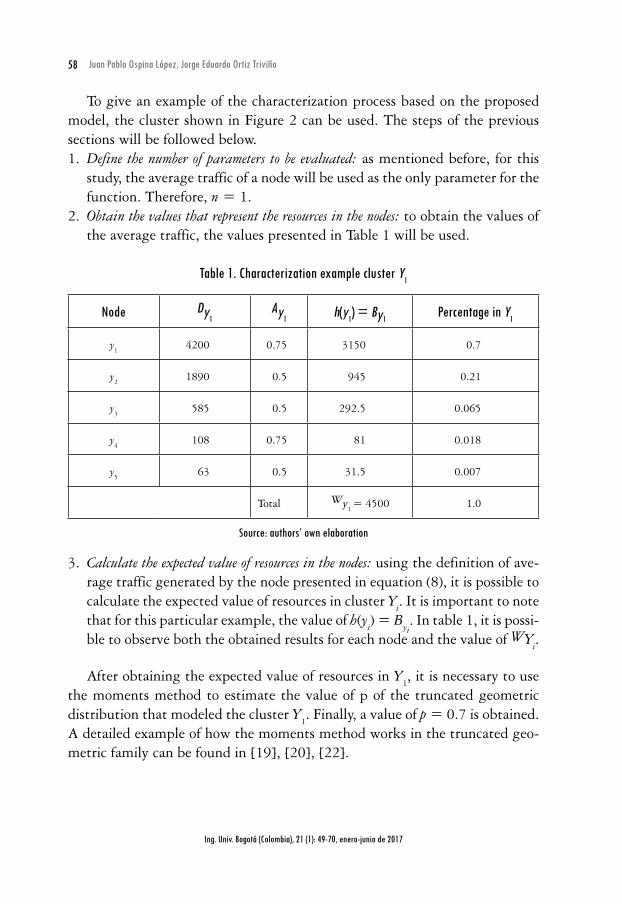
To give an example of the characterization process based on the proposed model, the cluster shown in Figure 2 can be used. The steps of the previous sections will be followed below.1. Define the number of parameters to be evaluated: as mentioned before, for this
study, the average traffic of a node will be used as the only parameter for the function. Therefore, n = 1.
2. Obtain the values that represent the resources in the nodes: to obtain the values of the average traffic, the values presented in Table 1 will be used.
Table 1. Characterization example cluster Y1
Node Dy1Ay1 h(y1) = By1 Percentage in Y1
y1
4200 0.75 3150 0.7
y2
1890 0.5 945 0.21
y3
585 0.5 292.5 0.065
y4
108 0.75 81 0.018
y5
63 0.5 31.5 0.007
Total Wy1 = 4500 1.0
Source: authors’ own elaboration
3. Calculate the expected value of resources in the nodes: using the definition of ave-rage traffic generated by the node presented in equation (8), it is possible to calculate the expected value of resources in cluster Yi. It is important to note that for this particular example, the value of h(yi) = Byi
. In table 1, it is possi-ble to observe both the obtained results for each node and the value of WYi.
After obtaining the expected value of resources in Y1, it is necessary to use
the moments method to estimate the value of p of the truncated geometric distribution that modeled the cluster Y
1. Finally, a value of p = 0.7 is obtained.
A detailed example of how the moments method works in the truncated geo-metric family can be found in [19], [20], [22].
59
Ing. Univ. Bogotá (Colombia), 21 (1): 49-70, enero-junio de 2017
Estimation of a growth factor to achieve scalable ad hoc networks
2. Results
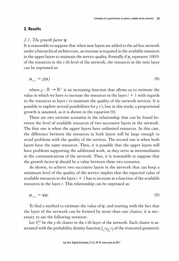
2.1. The growth factor jIt is reasonable to suppose that when new layers are added to the ad hoc network under a hierarchical architecture, an increase is required in the available resources in the upper layers to maintain the service quality. Formally if mi represent 100% of the resources in the i-th level of the network, the resources in the next layer can be expressed as:
mi+1 = g(mi) (8)
where g : → + is an increasing function that allows us to estimate the value in which we have to increase the resources in the layer i + 1 with regards to the resources in layer i to maintain the quality of the network services. It is possible to explore several possibilities for g (·), but in this study, a proportional growth is assumed, as it is shown in the equation (9).
There are two extreme scenarios in the relationship that can be found be-tween the level of available resources of two successive layers in the network. The first one is when the upper layers have unlimited resources. In this case, the difference between the resources in both layers will be large enough to avoid problems with the quality of the services. The second one is when both layers have the same resources. Then, it is possible that the upper layers will have problems supporting the additional work, as they serve as intermediaries in the communications of the network. Thus, it is reasonable to suppose that the growth factor j should be a value between these two scenarios.
As shown, to achieve two successive layers in the network that can keep a minimum level of the quality of the service implies that the expected value of available resources in the layer i + 1 has to increase as a function of the available resources in the layer i. This relationship can be expressed as:
mi+1 = jmi (9)
To find a method to estimate the value of j, and starting with the fact that the layer of the network can be formed by more than one cluster, it is nec-essary to use the following notation:
Let Yi(j) be the y-th cluster in the i-th layer of the network. Each cluster is as-
sociated with the probability density function fYi(j)(yi
(j)) of the truncated geometric
60
Ing. Univ. Bogotá (Colombia), 21 (1): 49-70, enero-junio de 2017
Juan Pablo Ospina López, Jorge Eduardo Ortiz Triviño
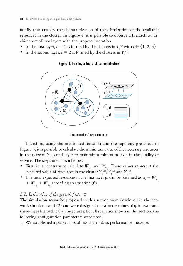
family that enables the characterization of the distribution of the available resources in the cluster. In Figure 4, it is possible to observe a hierarchical ar-chitecture of two layers with the proposed notation.• In the first layer, i = 1 is formed by the clusters in Y
1(j) with j ∈ {1, 2, 3}.
• In the second layer, i = 2 is formed by the clusters in Y2(1).
Figure 4. Two-layer hierarchical architecture
Layer 2
Layer 1Y2
(1)
Y1
(2)
Y1
(3)
Y1
(1)
Y2
(j)
Y1
(j)
Source: authors’ own elaboration
Therefore, using the mentioned notation and the topology presented in Figure 3, it is possible to calculate the minimum value of the necessary resources in the network’s second layer to maintain a minimum level in the quality of service. The steps are shown below:• First, it is necessary to calculate WY1
and WY3. These values represent the
expected value of resources in the cluster Y1(1), Y
1(2) and Y
1(3).
• The total expected resources in the first layer mi can be obtained as mi = WY1 + WY2
+ WY3 according to equation (6).
2.2. Estimation of the growth factor j The simulation scenarios proposed in this section were developed in the net-work simulator ns-3 [2] and were designed to estimate values of j in two- and three-layer hierarchical architectures. For all scenarios shown in this section, the following configuration parameters were used:1. We established a packet loss of less than 1% as performance measure.
61
Ing. Univ. Bogotá (Colombia), 21 (1): 49-70, enero-junio de 2017
Estimation of a growth factor to achieve scalable ad hoc networks
2. The operation of the cluster during the simulation was assumed to be sta-ble. Thus, there would be no changes in the network architecture or in the number of nodes in a cluster.
3. The stochastic model based on truncated geometric distribution proposed in section. 2.3 was used to determine the level of resources in each cluster of the network.
4. After finding a level of resources that satisfied the performance condition of the network, the growth factor was calculated to be =
μ2
μ1.
5. Finally, the mean of j, the standard deviation and a confidence interval with a level of significance of 5% through the t-Distribution (that was used due to the sample size) were calculated.
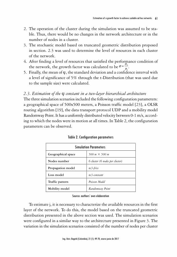
2.3. Estimation of the j constant in a two-layer hierarchical architectureThe three simulation scenarios included the following configuration parameters: a geographical space of 500x500 meters, a Poisson traffic model [23], a OLSR routing algorithm [19], the data transport protocol UDP and a mobility model Randomway Point. It has a uniformly distributed velocity between 0-1 m/s, accord-ing to which the nodes were in motion at all times. In Table 2, the configuration parameters can be observed.
Table 2. Configuration parameters
Simulation Parameters
Geographical space 500 m × 500 m
Nodes number 6 cluster (6 nodes per cluster)
Propagation model ns3-friss
Loss model ns3-constant
Traffic pattern Poisson Model
Mobility model Randomway Point
Source: authors’ own elaboration
To estimate j, it is necessary to characterize the available resources in the first layer of the network. To do this, the model based on the truncated geometric distribution presented in the above section was used. The simulation scenarios were configured in a similar way to the architecture presented in Figure 3. The variation in the simulation scenarios consisted of the number of nodes per cluster

62
Ing. Univ. Bogotá (Colombia), 21 (1): 49-70, enero-junio de 2017
Juan Pablo Ospina López, Jorge Eduardo Ortiz Triviño
and total number of clusters in the network. The architectures’ description and simulation results for the estimation process of j are presented in Table 3.
Table 3. j estimation phi results - Two-layer architectures
Description ˆ CI with a = 5%
1 6 clusters – 6 nodes per cluster 1.5057 [1.3988; 1.6162]
2 9 clusters – 4 nodes per cluster 1.5865 [1.4733; 1.6997]
3 4 clusters – 9 nodes per cluster 1.4245 [1.3147; 1.5442]
Source: authors’ own elaboration
These results let us suppose that the value of j for a two-layer architecture will be approximately 1.5 times the level of available resources in the first layer of the network. It is important to mention that these partial results were used to verify the behavior of the proposed model and the configuration of ns-3. An exhaustive analysis of hierarchical architectures of three layers is shown in the below section.
2.4. Estimation of the j constant in a three-layer hierarchical architecture The following aspects were considered for the estimation process of j in the three simulation scenarios proposed:1. To achieve a three-layer hierarchical architecture, a similar configuration
to that shown in Figure 3 was employed. We aggregated a third layer to serve as an intermediary in the communication process of two networks with hierarchical two-layer architectures.
2. The general configuration parameters to the network operation are shown in Table 1.
3. Bandwidths of 1,2,6,9,12,18 and 24 Mb were established as the available resource in the second layer of the network. After that, 20 simulations were performed for each bandwidth, and the results were analyzed through Weak Law of Large Numbers [19], [24] to determine the mean amount of resources in the third layer of the network.
4. Finally, a linear regression was made through the origin. The coefficient of determination and a confidence interval for j with a 5% significance were calculated for the purpose of validating the proposed model.

63
Ing. Univ. Bogotá (Colombia), 21 (1): 49-70, enero-junio de 2017
Estimation of a growth factor to achieve scalable ad hoc networks
2.4.1. Estimation process - Scenario 1
This scenario had 4 clusters with 6 nodes in the first layer and 2 clusters with 2 nodes in the second layer. In Table 4 and Figure 5 it is possible to observe the obtained results in the simulation process, as well as a confidence interval of 95% for values of m
1.
Figure 5. Three-layer hierarchical architecture – Scenario 1
25
20
15
10
5
0
Reso
urce
s lev
el 2
Resources level 10 2 4 6 8 10 12 14
y = 1.6906x
R 2 = 0.98713
Source: authors’ own elaboration
Table 4. Simulation results for the three-layer hierarchical architecture - Scenario 1
m1(Kbps) m2(Kbps) ˆ CI with a = 5% 1 740.7 1000 1.3501 [721.95; 759.44]
2 1340.4 2000 1.4921 [1294.60; 1386.19]
3 3938.4 6000 1.5235 [3875.08; 4001.71]
4 5413.2 9000 1.6626 [5328.00; 5498.49]
5 8217.1 12000 1.4604 [7934.91; 8499.33]
6 10218.45 18000 1.7615 [10076.11; 10360.78]
7 13673.15 24000 1.7553 [13456.11; 13890.12]
Source: authors’ own elaboration

64
Ing. Univ. Bogotá (Colombia), 21 (1): 49-70, enero-junio de 2017
Juan Pablo Ospina López, Jorge Eduardo Ortiz Triviño
2.4.2. Estimation process - Scenario 2
This scenario had 10 clusters with 3 nodes in the first layer and 8 clusters with 6 nodes in the second layer. In Table 5 and Figure 6, it is possible to observe the obtained results in the simulation process as well as a confidence interval of 95% for values m
1.
Figure 6. Three-layer hierarchical architecture – Scenario 2
25
20
15
10
5
0
Reso
urce
s lev
el 2
Resources level 10 2 4 6 8 10 12 14
y = 1.6471x
R2 = 0.98906
Source: authors’ own elaboration
Table 5. Simulation results for the three-layer hierarchical architecture - Scenario 2
m1 (Kbps) m2 (Kbps) ˆ CI with a = 5% 1 763.3 1000 1.3100 [734.34; 792.30]
2 1453.7 2000 1.3757 [1392.85; 1514.72]
3 3938.4 6000 1.3551 [4332.10; 4523.59]
4 5413.2 9000 1.4752 [6013.81; 6187.88]
5 8217.1 12000 1.5897 [7445.50; 7651.34]
6 10218.45 18000 1.6419 [10721.75; 11204.34]
7 13673.15 24000 1.7347 [13751.34; 13918.99]
Source: authors’ own elaboration
65
Ing. Univ. Bogotá (Colombia), 21 (1): 49-70, enero-junio de 2017
Estimation of a growth factor to achieve scalable ad hoc networks
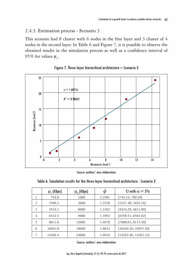
2.4.3. Estimation process - Scenario 3
This scenario had 8 cluster with 6 nodes in the first layer and 3 cluster of 4 nodes in the second layer. In Table 6 and Figure 7, it is possible to observe the obtained results in the simulation process as well as a confidence interval of 95% for values m
1.
Figure 7. Three-layer hierarchical architecture – Scenario 3
25
20
15
10
5
0
Reso
urce
s lev
el 2
Resources level 10 2 4 6 8 10 12 14
y = 1.6015x
R 2 = 0.98631
Source: authors’ own elaboration
Table 6. Simulation results for the three-layer hierarchical architecture - Scenario 3
m1 (Kbps) m2 (Kbps) ˆ CI with a = 5%1 794.8 1000 1.2581 [744.34; 790.30]
2 1596.3 2000 1.2528 [1547.48; 1645.24]
3 4524.1 6000 1.3262 [4434.29; 4613.90]
4 6432.3 9000 1.3992 [6358.51; 6563.02]
5 8011.8 12000 1.4978 [7908.63; 8115.30]
6 10692.8 18000 1.6834 [10430.39; 10955.30]
7 14449.4 24000 1.6610 [14262.46; 14363.33]
Source: authors’ own elaboration
66
Ing. Univ. Bogotá (Colombia), 21 (1): 49-70, enero-junio de 2017
Juan Pablo Ospina López, Jorge Eduardo Ortiz Triviño
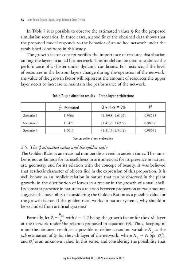
In Table 7 it is possible to observe the estimated values φ for the proposed simulation scenarios. In three cases, a good fit of the obtained data shows that the proposed model responds to the behavior of an ad hoc network under the established conditions in this study.
The growth factor concept verifies the importance of resource distribution among the layers in an ad hoc network. This model can be used to stabilize the performance of a cluster under dynamic conditions. For instance, if the level of resources in the bottom layers change during the operation of the network, the value of the growth factor will represent the amount of resources the upper layer needs to increase to maintain the performance of the network.
Table 7. j estimation results – Three-layer architecture
ˆ - Estimated CI with a = 5% R 2
Scenario 1 1.6906 [1.3988; 1.6162] 0.98713
Scenario 2 1.6471 [1.4733; 1.6997] 0.98906
Scenario 3 1.6015 [1.3147; 1.5442] 0.98631
Source: authors’ own elaboration
2.5. The φ estimated value and the golden ratio The Golden Ratio is an irrational number discovered in ancient times. The num-ber is not as famous for its usefulness in arithmetic as for its presence in nature, art, geometry and for its relation with the concept of beauty. It was believed that aesthetic character of objects lied in the expression of this proportion. It is well known as an implicit relation in nature that can be observed in the plant growth, in the distribution of leaves in a tree or in the growth of a snail shell. Its constant presence in nature as a relation between proportion of two amounts suggests the possibility of considering the Golden Ration as a possible value for the growth factor. If the golden ratio works in nature systems, why should it be excluded from artificial systems?
Formally, let i =μi+1
μi with i = 1,2 being the growth factor for the i-th layer
of the network under the relation proposed in equation (9). Thus, keeping in mind the obtained result, it is possible to define a random variable Xij as the j.th estimation of ji for the i-th layer of the network, where Xij ~ N (ji, σi
2), and σi
2 is an unknown value. In this sense, and considering the possibility that

67
Ing. Univ. Bogotá (Colombia), 21 (1): 49-70, enero-junio de 2017
Estimation of a growth factor to achieve scalable ad hoc networks
the growth factor can be related to the Golden Ratio, the following hypotheses were proposed:
H0 : i =1+ 5
2
H1 : i =1+ 5
2
A confidence interval I = X tn 1( ), 2
Sn
, X + tn 1( ),a2
Sn
with a = 5% constructed from Student’s t-test distributions were then used [22] for each of the simulation scenarios proposed in this research, as shown in Table 7. These results indicate the lack of evidence for rejecting H
0. Therefore, it is possible to consider that the
value of =1+ 5
2 corresponds to the growth factor proposed in equation (9), with
a = 5%. This value opens the possibility to determine the best relationship between the level of resources in two successive layers of the ad hoc network.
3. ConclusionsThe massive use of wireless devices makes it necessary to develop mechanisms to handle large amounts of nodes without losing quality in the services offered by the communication networks. Achieving scalability in ad hoc networks is a challenge in the design of protocols, and so it is a necessary condition to obtain ad hoc networks with high deployability.
A model based on the truncated geometric distribution was proposed to char-acterize the level of resources in an ad hoc network under a hierarchical archi-tecture. This model makes it possible to determine the level of heterogeneity in a cluster to classify the nodes in terms of their resources.
A growth factor was proposed as a constant value that represents the suit-able relationship between the level of resources in two successive layers of the network. This relationship can be modeled like a proportional growth between the resources and the performance metrics of the network. This result can be useful to complement the clustering algorithms through metric combination and help to maintain the cluster in a stable condition when there are frequent changes in the amount of the resources in the network.
The growth factor j was estimated through simulation for the hierarchical architectures of two and three layers, finding a value of =
1+ 52
with a confidence level of 95%. A similarity between the growth factor and the Golden Ratio was

68
Ing. Univ. Bogotá (Colombia), 21 (1): 49-70, enero-junio de 2017
Juan Pablo Ospina López, Jorge Eduardo Ortiz Triviño
shown as way to inspire the design process of artificial systems based on attributes found in nature. The determination coefficients obtained from the simulation scenarios show a good fit of the results to the proposed model.
This investigation can be considered as an extended version of the work published in [1], [2]. The main contributions of this paper were the verification of the value of the growth factor for two-layer hierarchical architectures and the exploration of its behavior for three-layer hierarchical architectures. Additionally, we showed through simulation results that it is possible to model the relationship between two successive layers of the network as a linear model.
In future work we expect to explore the behavior of the growth factor in an ad hoc network with self-similar traffic. This type of traffic appears in wireless networks with different services. We want to explore how the value of the growth factor changes when the ad hoc network can support different traffic flows, each one with different performance metrics.
References[1] J. Ospina and J. Ortiz, “Stochastic model for the characterization of a cluster and its re-
sources in an ad-hoc network,” In Communications and Computing (COLCOM), 2014 IEEE Colombian Conference on (pp. 1-5), IEEE, 2014.
[2] J. Ospina, H. Zarate, and J. Ortiz, “Scalability in ad hoc networks under hierarchical archi-tectures,” In Communications and Computing (COLCOM), 2015 IEEE Colombian Conference on (pp. 1-6). IEEE, 2015.
[3] P. Ghosekar, G. Katkar, and P. Ghorpade, “Mobile ad hoc networking: imperatives and challenges,” IJCA Special Issue on MANETs, vol. 3, pp. 153-158, 2010.
[4] J. Loo, J. Mauri, and J. Ortiz, Mobile ad hoc networks: current status and future trends. Boca Raton: CRC Press, 2016.
[5] S. Reddy, D. Estrin, and M. Srivastava, Emerging Wireless Technologies and the Future Mobile Internet. Cambridge: Cambridge University Press, 2011.
[6] D. Raychaudhuri and N. Mandayam, “Frontiers of wireless and mobile communications,” Proce. IEEE, vol. 100, no. 4, pp. 824-840, 2012.
[7] D. Tschopp, S. Diggavi, and M. Grossglauser, “Hierarchical routing over dynamic wireless networks,” In ACM SIGMETRICS Performance Evaluation Review, vol. 36, no. 1, pp. 73-84, 2015.
[8] P. Gupta and P. Kumar, “The capacity of wireless networks,” IEEE Trans. Inf. Theory, vol. 46, no. 2, pp. 388-404, 2000.
[9] J. Yu and P. Chong, “A survey of clustering schemes for mobile ad hoc networks,” IEEE Commun. Surveys Tuts., vol. 7, no. 1, pp. 32-48, 2005.

69
Ing. Univ. Bogotá (Colombia), 21 (1): 49-70, enero-junio de 2017
Estimation of a growth factor to achieve scalable ad hoc networks
[10] K. Abboud and W. Zhuang, “Stochastic modeling of single-hop cluster stability in vehi-cular ad hoc networks,” IEEE Trans. Veh. Technol., vol. 65, no. 1, p. 226-240, 2016.
[11] J. Ospina and J. Ortiz, “Scalability in ad hoc networks: the effects of its complex nature,” Int. J. Eng. Technol., vol. 3, no. 3, p. 315, 2014.
[12] M. Grossglauser and D. Tse, “Mobility increases the capacity of ad-hoc wireless networks,” Twentieth Annual Joint Conference of the IEEE Computer and Communications Societies Proceedings. IEEE, vol. 3, pp. 1360-1369, 2001.
[13] R. Ramanathan, R. Allan, and P. Basu, “Scalability of mobile ad hoc networks: Theory vs practice,” In Military Communications Conference, 2010-MILCOM 2010 (pp. 493-498). IEEE, 2010.
[14] D. Palma and M. Curado, “Scalability and routing performance of future autonomous networks,” Int. Journal Internet Protocol Technol., vol. , no. 3, pp. 137-147, 2013.
[15] A. Boukerche, B. Turgut, N. Aydin, M. Ahmad, and L. Bölöni, “Routing protocols in ad hoc networks: a survey. Computer Networks, vol. 55, no. 13, pp. 3032-3080, 2011.
[16] I. Ouafaa, L. Jalal, K. Salah-ddine, and E. H. Said, “The comparison study of hierarchical routing protocols for ad-hoc and wireless sensor networks: A literature survey,” Proceedings of the the International Conference on Engineering & MIS 2015, 2015, p. 32.
[17] M. Chatterjee, S. Das, and D. Turgut, “WCA: A weighted clustering algorithm for mobile ad hoc networks,” Cluster Computing, vol. 5, no. 2, pp. 193-204, 2002.
[18] W. Zhu, D. Gao, A. Fong, and F. Tian, “An analysis of performance in a hierarchical structured vehicular ad hoc network,” Int. J. Distributed Sensor Networks, p. 969346, 2014. http://dx.doi.org/10.1155/2014/969346
[19] S. Ross, Introduction to probability models, New York: Academic Press, 2014. [20] V. Iversen, Teletraffic engineering and network planning, Lyngby: Technical University of
Denmark, 2015. [21] G. Riley and T. Henderson, “The ns-3 network simulator,” In Modeling and Tools for Network
Simulation (pp. 15-34). Berlin: Springer-Heidelberg, 2010. [22] S. Searle, Linear models, New York: Springer, 1971.[23] T. Clausen, P. Jacquet, C. Adjih, A. Laouiti, and P. Minet, “Optimized link state routing
protocol (OLSR),” (no. RFC 3626), 2003. [24] A. Mood, Introduction to the Theory of Statistics, New York: McGraw Hill, 1950.
