GeoConvention 2020 1

Estimation of Acoustic Impedance from Seismic Data in Well-log Resolution Using Machine Learning, Neural Network, and Comparison with Band-limited Seismic Inversion

Ryan A. Mardani

Geo Vision Thrust

Summary

Acoustic Impedance is one of the most important rock properties that can be extracted from surface seismic data using inverse theory. Conventional seismic inversion results are highly dependent on seismic data frequency content, leading to resolution limitation. The objective of this study is to look for another possible approach to estimate impedance in better resolution. From various machine learning approaches, Artificial Neural Network (ANN), mimics neuron cells to train the network to minimize the error between network output and target data. In this work, after trying several seismic attributes, five of them (second derivative, quadrature amplitude, trace gradient, gradient magnitude and instantaneous frequency) are used to train the network to have estimation of impedance. The aim of this network is to find seismic-related inputs to predict impedance in well log resolution along the area of study. Impedance estimation was carried out with 88% correlation. Recursive seismic inversion was also implemented using well logs and post stack time migrated seismic data. The comparison between neural network and seismic inversion results illustrates that machine learning can work accurately to estimate impedance even with better resolution which seismic data is limited to band of ≈ 8 to 80 Hz, though it is computationally expensive.

Workflow & Methodology

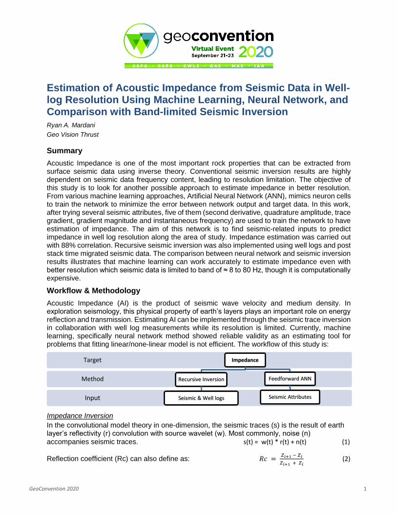
Acoustic Impedance (AI) is the product of seismic wave velocity and medium density. In exploration seismology, this physical property of earth’s layers plays an important role on energy reflection and transmission. Estimating AI can be implemented through the seismic trace inversion in collaboration with well log measurements while its resolution is limited. Currently, machine learning, specifically neural network method showed reliable validity as an estimating tool for problems that fitting linear/none-linear model is not efficient. The workflow of this study is:

Impedance Inversion

In the convolutional model theory in one-dimension, the seismic traces (s) is the result of earth layer’s reflectivity (r) convolution with source wavelet (w). Most commonly, noise (n)

accompanies seismic traces. s(t) = w(t) * r(t) + n(t) (1)

Reflection coefficient (Rc) can also define as: 𝑅𝑐 = 𝑍𝑖+1 − 𝑍𝑖

𝑍𝑖+1 + 𝑍𝑖 (2)

Input

Method

Target Impedance

Recursive Inversion

Seismic & Well logs

Feedforward ANN

Seismic Attributes

GeoConvention 2020 2

where Z is equal to compressional wave velocity multiplied by density. Solving for 𝑍𝑖+1 ,

𝑍𝑖+1 = 1+ 𝑅𝑐

1− 𝑅𝑐 𝑍𝑖 (3)

This means that knowledge of upper layer impedance and reflectivity value between two layers can lead us to impedance of next layer. This is the simplest and oldest method of inversion carrying the following issues:

The inversion result is band-limited (in surface seismic frequency content ~ 10 to 50 Hz)

It algorithms accepts zero-phase seismicWavelet effect on seismic trace is neglected while reflectivity is convolved with source wavelet in seismic traces

Multilayer Neural Network Backpropagation Training This network architecture can fit the best for our purposes as there is some clue from target data known as impedance. Each network will receive input data, which will have especial importance in network called weight, w. Bias, b, works as threshold to whether pass the message to next neuron or not. Finally, activation, a, which will be passed to next neuron needs to have transfer function applied to it, f, to make special range for the data. This data is sum of bias and product of weight and input data. In fact, activation works as input to next layer. At the first iteration (here called epochs) Weight will be randomly (Gaussian distribution) chosen by system. In the second iteration training will start to minimize the differences between calculated prediction data with target data (cost function) which we already feed the network. In fact, the adjustment will focused on weight and bias to the get the most similar result to target data.

𝐶(𝑤, 𝑏) =1

2𝑛∑ ||𝑦(𝑥) − 𝑎||2

𝑥 (4)

where C is cost function which is function of weight and bias, y is target data and a is result of network as output (Nielsen, 2015). Training can be instructed in different ways. Any kinds of optimization function can be applied in training neural networks but few of them are efficient especially those that optimizing gradient of network performance with respect to weight or those that optimizing Jacobian of the network errors. These two parameters are calculated using Backpropagation algorithm which works backward in network (Demuth et.al, 2009).

Results Let’s first generate conventional seismic inversion results. After loading check-shot data in well places, sonic log is corrected with well velocity and low frequency velocity model is established. Band limited inversion is implemented using Hampson-Russell software. Basically, it assumes the seismic reflection amplitude as reflectivity series (though we may apply various kind of deconvolution to get rid of wavelet imprint from seismic traces). Well logs provides important information regarding impedance at the starting point of inversion.

In the second track from left (figure1), the inversion result (in red) is overlaying the original impedance log from the well (blue). In the next track, we see the selected wavelet (in blue) and the synthetic traces calculated from this inversion result (in red) followed by the original seismic composite trace (in black). Higher correlation shows the error is practically low, indicating that the inversion is mathematically correct. This inversion creates a synthetic trace which matches the real trace. In this picture, resolution differences can be seen clearly.

In the next step, we investigate an approach that help us to estimate impedance variations just by employing surface seismic data but in finer scale (well log resolution). In fact, we need to

GeoConvention 2020 3

examine that how strong and how independent the neural network can be trained to predict impedance from seismic data. Several types of seismic attributes were created and the best input training attributes are chosen as: Second derivative, Quadrature amplitude, Trace gradient, Gradient magnitude, Instantaneous frequency (for more explanation refer to Appendix).

Figure 1: seismic inversion result in left track (red) is overlaid with log-calculated impedance (blue). Zero-phase wavelet extracted from entire seismic cube is shown in next track. Using impedance from inversion result, reflectivity extracted then convolved with wavelet to generate synthetic track (red). High correlation with real seismic amplitude profile can be interpreted as inversion accuracy.

The plot of these training set and target can be seen in figure 2. Operationally, there are several factors that control cost of calculation including: number of attributes as input training, number of hidden layers and nodes in each layer and number of data points (in other word sample rate). It is recommended to start with simple network structures and then approach to optimal design. Using TensorFlow library in python programing, it is gained the following optimum network: 2 hidden layers where each contains 100 and 50 neurons, respectively. The data matrix size is (30,000×6) which is divided into 70% for training and the rest for validation and test.

Figure2: this figure illustrates zero-offset seismic trace in one well location in first track, left. Training input attributes is extracted from seismic traces for all wells as Second derivative, Quadrature amplitude, Trace gradient, Gradient magnitude and Instantaneous frequency. The target of network is AI.

GeoConvention 2020 4

Although iteration was programed into 1500 cycle of calculation for error minimization, model

starts to overfitting after epoch 200. To avoid such problem, early stopping is enforced when

validation error starts to build up in certain amounts (figure 3, left). Epoch 70 seems appropriate

selection for training. Having built model, we may examine model accuracy on test data. True AI

is in agreement with prediction output from model by 88% correlation coefficient (figure 3, middle).

Error has zero mean Gaussian distribution (figure 3, right).

Figure 3: Mean absolute error (MAE) decay through training period (left). After epoch 70, training would

not add accuracy in validation dataset. In the middle plot, correlation coefficient between real data and

model prediction is 88% and the error has zero mean normal distribution (right).

Finally, plotting real acoustic impedance in well place with seismic-derived ANN impedance shows strong agreement between these two data sets (figure 4). For comparison, band-limited inversion results is also overlaid. After all, neural network like other mathematical approaches is sensitive to the noise in input data. In fact, the high level of noise can cause network to be trained for noisy predictions. It is not recommended but possible to remove some outliers from input data. Like human brain, learning level can be proportional to how wide range of learning data is offered. It is better to have plenty of data range with redundant data samples. Computation cost is directly related to amount of input data, network layers and neurons. As these parameters increases, the estimation accuracy will increase but training process will be time consuming process.

Figure4: Predicted and real AI are plotted in reservoir intervals in well place. The trend and values show strong agreement. Band limited inversion impedance is also plotted to see how it follows the property variation through the depth. Overall, it shows appropriate trend adaptation but for local variation it does not have enough ability to extract the same resolution.

GeoConvention 2020 5

Conclusion

The main purpose of this study was to investigate the possibility of other approaches rather

inversion to estimate impedance using seismic and well data. It is tried to estimate AI using

seismic data attributes as input to target AI. A network with two hidden layers (100 and 50 neurons

in each layer, respectively) is trained employing TensorFlow library deep learning in python

platform. These selected five attributes are: second derivative, quadrature amplitude, trace

gradient, gradient magnitude and instantaneous frequency. The network could recognized

appropriate relationship (correlation of 88%) between these seismic attributes and target data as

impedance. Band-limited seismic inversion was also implemented and inversion result was

compared with network estimation. The comparison illustrates that neural network can work

effectively to estimate impedance even with more detail than band-limited seismic inversion

because the network inherits target data frequency while recursive inversion is limited to seismic

band frequency, although it is expensive approach.

References

- Barnes, A. E., 2016, Handbook of poststack seismic attributes: SEG Geophysical Reference Series 21.

- Demuth, H., Beale, M., Hagan, M., 2009, “Neural Network Toolbox™ 6 User’s Guide” : MATHWORKS

- Hagan, M.T., and M. Menhaj, “Training feed-forward networks with the Marquardt algorithm,” IEEE Transactions

on Neural Networks, Vol. 5, No. 6, 1999, pp. 989–993, 1994.

- Russell, B., 1988, Introduction to seismic inversion methods: SEG

APPENDIX:

Second derivative: it is the second time derivative of the input seismic volume. This can work as helpful tools for interpreters in the places where continuity is poorly resolved on raw amplitude profiles (Barnes, 2016).

Quadrature amplitude: this attribute is the imaginary part of the analytic signal, which is calculated by phase shifting the original trace by 90 degrees. An analytic signal can be generated from the real seismic amplitude and the imaginary quadrature amplitude (Barnes, 2016).

Trace gradient: the gradient along the trace is calculated. It will have the highest values where the greatest changes are happening (Barnes, 2016).

Gradient magnitude: the magnitude of instantaneous gradient is computed in 3-dimention employing neighbor traces (Barnes, 2016).

Instantaneous frequency: it is the time derivative of phase angle and different from wavelet frequency. Commonly is used to estimate seismic attenuation. It can show cyclicity of geological features to assist interpretation. Reservoir oil and gas fluids may cause drop-off of high frequency components (Barnes, 2016).