estimation of an agent-based model of investor sentiment formation in financial markets

Contents lists available at SciVerse ScienceDirect

Journal of Economic Dynamics & Control

Journal of Economic Dynamics & Control 36 (2012) 1284–1302

0165-18

http://d

n Corr

E-m

journal homepage: www.elsevier.com/locate/jedc

Estimation of an agent-based model of investor sentimentformation in financial markets

Thomas Lux a,b,c,n

a Department of Economics, University of Kiel, Kiel, Germanyb Kiel Institute for the World Economy, Kiel, Germanyc Bank of Spain Chair of Computational Economics, Department of Economics, University Jaume I, Castellon, Spain

a r t i c l e i n f o

Article history:

Received 17 April 2011

Accepted 26 September 2011Available online 30 March 2012

JEL classification:

G12

G17

P84

Keywords:

Opinion formation

Social interaction

Investor sentiment

89/$ - see front matter & 2012 Elsevier B.V. A

x.doi.org/10.1016/j.jedc.2012.03.012

espondence address: Department of Econom

ail address: [email protected]

a b s t r a c t

We use weekly survey data on short-term and medium-term sentiment of German

investors to estimate the parameters of a stochastic model of opinion formation

governed by social interactions. The bivariate nature of our data set also allows us to

explore the interaction between the two hypothesized opinion formation processes,

while consideration of the simultaneous weekly changes of the stock index DAX enables

us to study the influence of sentiment on returns. Technically, we extend the maximum

likelihood framework for parameter estimation in agent-based models introduced by

Lux (2009a) by generalizing it to bivariate and tri-variate settings. As it turns out, our

results are consistent with strong social interaction in short-run sentiment. While one

observes abrupt changes of mood in short-run sentiment, medium-term sentiment is a

more slowly moving process in which the influence of social interaction seems to be

less pronounced. The tri-variate model entails a significant effect from short-run

sentiment on prices in-sample, but its out-of-sample predictive performance does not

beat the random walk benchmark.

& 2012 Elsevier B.V. All rights reserved.

1. Introduction

Opinion dynamics in financial markets have been modeled by Topol (1991), Kirman (1993), Lux (1995, 1998) andAlfarano et al. (2008) among others. These models make use of epidemic processes of information transmission betweenagents that allow for an endogenous formation of expectations. Markets with such interacting speculators give easily riseto speculative bubbles, crashes and excess volatility, and therefore, provide an avenue towards an explanation of theseubiquitous phenomena. Perhaps even more important, a certain number of these agent-based models has also been shownto exhibit more fundamental statistical properties of financial returns: Models like those proposed by Lux and Marchesi(1999, 2000), Iori (2002) or Pape (2007) generate time series that replicate the well-known stylized facts like fat tails andclustered volatility, even up to close numerical proximity of key empirical statistics of financial data (cf. Lux, 2009b, for anoverview of this literature).

Our aim in this paper is to estimate the parameters of an agent-based model of opinion formation and its impact onprices. This goal means that we attempt to identify structural parameters of an agent-based model (ABM) from aggregatedata. The literature on estimation of ABMs has got started only recently and pertinent contributions are still scarce. Early

ll rights reserved.

ics, University of Kiel, Olshausen Strasse 40, 24118 Kiel, Germany.

www.elsevier.com/locate/jedc

www.elsevier.com/locate/jedc

dx.doi.org/10.1016/j.jedc.2012.03.012

mailto:[email protected]

dx.doi.org/10.1016/j.jedc.2012.03.012

dx.doi.org/10.1016/j.jedc.2012.03.012

T. Lux / Journal of Economic Dynamics & Control 36 (2012) 1284–1302 1285

research in this vein has concentrated on regime-switching models with two regimes accounting for periods of dominatingchartist or fundamentalist influence in financial markets. Examples include Vigfusson (1997) and Westerhoff and Reitz(2003). While the former reports weakly favorable results for a chartist and fundamentalist framework, the latter authorsfind that fundamentalists’ reactions might not be sufficiently strong to prevent amplification of distortions in the foreignexchange market. More recent contributions have also started to estimate heterogeneous agent models with performance-based switching rules for the choice of strategies or predictor functions. Boswijk et al. (2007) estimate a dynamic assetpricing model with heterogeneous, boundedly rational agents. In this model, a discrete choice-style selection mechanismbased on past profits governs agents’ switching between a fundamentalist and a chartist predictor. They estimate thismodel via nonlinear least squares for yearly data of the U.S. stock market from 1871 until 2003 and find that they canreject a benchmark linear asset-pricing model against the nonlinear two-group framework. Belief coefficients are stronglysignificant and indicate the prevalence of different strategies among market participants.

Somewhat less clear-cut evidence for the explanatory power of a similar ABS model is reported for daily stock indexdata by Amilon (2008). This author points out that replication of stylized facts like volatility clustering hinges on thespecification of the noise term while the nonlinearity introduced via the structural ABM model does not contribute muchto the overall fit of the model. Franke (2009), in contrast, obtains a better fit of a simple ABM framework to selectedmoments that capture important stylized facts.

A similar approach has been pursued by Goldbaum and Mizrach (2008) who adopt the discrete-choice approach tomutual fund allocation decisions. On the base of 10 years of data on inflow of capital to actively and passively managedfunds, they estimate a discrete-choice model on the base of utility differences of investors from the active or passivevarieties. They find that about 80% of the variation of fund flows can be explained by the model. A discrete-choiceframework for the choice of expectation formation rules for inflation forecasts has been studied by Branch (2004). Usingmicro data from the Michigan Survey of Consumer Attitudes and Behavior, he finds significant evidence of heterogeneityamong respondents. Allowing for the possibilities of vector autoregressive, adaptive and naive expectations, Branch findsthat the respondents’ choice of predictors reacts negatively to mean squared prediction error.

ABM models with contagious interpersonal communication have been estimated by Gilli and Winker (2003), Alfaranoet al. (2005), Klein et al. (2008), Franke (2008) and Lux (2009a). Gilli and Winker (2003) estimate the ‘‘ant’’ model ofpairwise exchange of information of Kirman (1993) for foreign exchange data and find evidence for bi-modality, i.e.changes between dominance of both underlying opinions (chartist and fundamentalist predictors in the application to a foreignexchange market). Alfarano et al. (2005) estimate the parameters of a closely related model with asymmetric switchingpropensities and find that different markets are governed by different prevailing tendencies towards fundamentalist or chartistbehavior. Klein et al. (2008) attempt to estimate the more involved model by Lux and Marchesi (1999) that combines thechartist-fundamentalist dichotomy with social interactions among agents. While they do not report parameter estimates, theyprovide results on the estimated fraction of chartists as it develops over time. Results appear to be in good harmony withhistorical perceptions of the financial history over the last 60 years.

Closest to our current paper are the recent contributions by Franke (2008) and Lux (2009a) who attempt to estimate theparameters of models of social opinion formation among agents for economic sentiment data. Our goal in this paper is togo one (or two) steps beyond a previous paper (Lux, 2009a) that introduced a method for identification of the parametersof microscopic opinion processes from aggregate data. This paper, however, was confined to estimation of the parametersof a model for a univariate time series, namely the diffusion index form (number of optimistic individuals minus numberof pessimistic individuals) of a business climate survey. While the same model and estimation methodology could beapplied for financial sentiment data (which often share the format of diffusion indices), a univariate model would onlyallow us to cover one of the building blocks of the above asset pricing models. As a minimum requirement, however, for anempirical validation of a stochastic behavioral asset pricing model one would like to study the joint dynamics of assetprices and sentiment. We will, therefore, extend our previous model into this direction and provide parameter estimatesfor a simple version of a simultaneous system. Since our underlying time series cover two sentiment variables, one for theshort horizon and one for the medium-term horizon, we can even go one step further and study two interacting opinionprocesses together with the time development of the asset price. Since this amounts to studying the dynamics of a tri-variate series, we proceed in this paper from the 1D case of Lux (2009a) to the 2D and 3D cases. As in the previous paper,the methodology presented below could be applied to a wide variety of hypothesized opinion dynamics interacting withobjective economic variables. In order to demonstrate the practical use of estimated agent-based models, we also performan out-of-sample forecasting experiment based on our estimated models.

Apart from the still relatively sparse literature on estimation of agent-based models our approach could also be linkedto a much more voluminous strand of empirical research: Empirical models of survey measures of sentiment orinvestment (business, consumer) climate. Since we will use a diffusion approximation to our underlying opinion process,we could also interpret our exercise as estimation of a time series model motivated by an agent-based model. Sentimentindices could be considered as risk factors in the asset pricing equation in such a setting. Our research would, then, explorethe added explanatory power of nonlinearities introduced through the interaction of agents while previous research hasmainly used linear models for modeling sentiment and its explanatory power as a risk factor for stock price movements(cf. Brown and Cliff, 2004; Schmeling, 2009).

The rest of the paper is structured as follows: In Section 2 we introduce our stochastic framework of sentimentdynamics and simultaneous price changes. Section 3 provides details on our estimation methodology, maximum

T. Lux / Journal of Economic Dynamics & Control 36 (2012) 1284–13021286

likelihood estimation based on a numerical approximation of the transient density of the underlying stochastic process.Section 4 gives details on the sentiment data we use as well as an overview on previous findings on the interactionbetween sentiment and returns within a non-behavioral VAR framework. In Section 5 we present results for univariatepopulation dynamics and diffusion processes for each one of our three time series. In Sections 6 and 7 we proceed tovarious combinations of 2D models and the full-fletched model of three simultaneous stochastic processes. Section 8summarizes our findings and concludes. The Appendix provides details on the numerical approximation schemes for thedynamics of the transient density.

2. The joint dynamics of asset prices and sentiment

For the group dynamics that govern the time development of traders’ mood, we adopt the Weidlich model of opinionformation (Weidlich and Haag, 1983; Weidlich, 2000; Lux, 1995): agents have the choice of voicing one of two opinions,denoted here by ‘‘þ ’’ and ‘‘� ’’ (optimistic and pessimistic). Agents change their beliefs in continuous time, with a Poissonprocess formalizing the switches from the ‘‘þ ’’ to the ‘‘� ’’ group and vice versa within the next instant. The pertinenttransition rates are denoted by om and ok and assume an exponential functional form

om ¼ n expðUÞ, ok ¼ n expð�UÞ: ð1Þ

here n is a scale parameter that determines the frequency of transitions, and the function U covers those determinants thatmight exert an influence on agents’ decisions to change their belief. In our present application we assume that our twosentiment variables, say x (short-run sentiment) and y (medium-run sentiment) are both determined via a similarepidemic opinion process. We denote by ws

mðwskÞ and om

m ðomk Þ the transition rates for short-run and medium-run

sentiment, respectively. Allowing for cross-dependencies between both processes as well as for dependency on returnsðretÞ, we specify the pertinent rates of Eq. (1) as

osm ¼ ns expðU1Þ, os

k ¼ ns expð�U1Þ ð2Þ

with

U1 ¼ a0þa1xþa2yþa3ret

for the dynamics governing short-run sentiment and

omm ¼ nm expðU2Þ, om

k ¼ nm expð�U2Þ ð3Þ

with

U2 ¼ b0þb1yþb2xþb3ret

for the dynamic evolution of medium-run sentiment. We denote the number of optimistic (pessimistic) individuals in theshort-run index by nþ and n�, and the optimists (pessimists) in the medium-term index by mþ and m�, respectively. Theempirical series, therefore, correspond to

x¼nþ�n�

2N, y¼

mþ�m�2M

ð4Þ

with 2Nð2MÞ the total number of respondents.1 Since we do not have exact information on response rates, N and M are theparameters that will also be estimated in our empirical exercise. The reason is that, on the one hand, we only have roughorders of magnitude for the numbers of participants: According to the provider of our data set, average response rates are20–25% of a pool of about 2000 subscribers. On the other hand, it might well be that our model does not capture all typesof interaction. There might be groups of agents who are exposed to the same factors of influence and might actually exhibitperfectly synchronous behavior, instead of the conditionally independent transition rates of Eqs. (2) and (3). Since suchhomogeneous behavior would reduce the number of ‘effectively’ independent respondents, we would expect our model tofit better with a smaller number of agents than the nominal one under such circumstances. Note that our goal is more toexplore whether the model provides a good fit of the macroscopic dynamics and not so much whether it is a goodformalization of individual behavior.

Note that our agent-based model consists of 2Nþ2M coupled Markov processes for agents’ belief dynamics incontinuous time. In previous work, theoretical results on closely related models have been obtained via approximatedynamics of mean values and higher moments (Lux, 1995, 1998; Alfarano et al., 2008). For a single opinion process, theaggregate outcome of the process hinges crucially on a1 (or b1): if this parameter (that could be labeled the intensity ofherding or interaction) is below 1, the stationary distribution has a unique maximum, while it becomes bi-modal understronger interaction (a141 or b141). The latter case allows for the build-up and breakdown of strongly optimistic orpessimistic majorities and depending on the parameters ns and nm, a rapid change between one type and the other. Withtwo interacting opinion processes, the picture becomes more complex and also allows for cyclical behavior besides theuni-modal and bi-modal scenarios (cf. Weidlich, 2000, chapter 4).

1 The factor 2 is introduced for convenience to make sure that the population size is even allowing for the possibility of a neutral average mood

x¼0 or y¼0.


Since we found some indication that our baseline opinion process could be overparametrized for the medium-termindex,2 we also tried a model in which this population dynamics was replaced by a simple diffusion equation of theOrnstein–Uhlenbeck (OU) type:

dyt ¼ kðyþb1xtþb2rett�ytÞ dtþsy dZ1 ð5Þ

with dZ1 a standard Brownian motion. This variant assumes that medium-term sentiment is a mean-reverting process thatis also influenced by the current state of short-term sentiment and contemporaneous returns.

In order to study the influence of sentiment on price movements, we add another diffusion process for the dynamics ofthe stock index (denoted by pt):

dpt ¼ ðg0þg1xtþg2ytÞ dtþsp dZ2: ð6Þ

Note that for g1 ¼ g2 ¼ 0, (6) becomes a standard Brownian motion with drift. Significant parameter estimates of g1 or g2

would indicate an influence of sentiment on price changes that could be exploited for prediction of near-term returns. Wehave also estimated additional squared terms in the drift function but these turned out to be uniformly insignificant.Similarly, a more flexible diffusion function has been tried, but did not contribute any additional explanatory power to thesimpler specification. Following similar specifications in the time series literature on sentiment, time-variation in thediffusion term was accommodated by adding dependence on absolute values of sentiment indicators (as proxies formarket activity), but the pertinent parameters were also nowhere close to significant.

It might appear disturbing that the pricing Eq. (6) does not include a fundamental value as an anchor that preventsprices from ‘drifting to idiocy’ (as a referee put it). Indeed, agent-based models of financial markets typically include suchan anchor (cf. Lux, 1995; Iori, 2002; Pape, 2007). Note, however, that such an anchor is not needed because of the empiricalnature of our work in which we are mainly interested in the influence of sentiment factors on top of changes offundamental factors. While one would certainly need an anchor in a simulation study, the empirical data are save fromhaving ‘drifted to idiocy’ per se. As an aside, our companion paper (Lux, 2010) shows that medium-run sentimentencapsulates the information from most of the usual fundamental asset-pricing factors.

3. Estimation methodology

Lux (2009a) has developed a numerical maximum likelihood approach for a univariate population process. For discreteaggregate observations of an opinion index, the conditioned likelihood of each observation, conditional on last period’srealization, can be obtained from numerical solutions of the so-called Fokker–Planck equation. The Fokker–Planck equation orforward Kolmogorov equation gives the time evolution of the probability density function of a stochastic system. For diffusionfunctions, the Fokker–Planck equation is the exact law of motion for the transitional density, while it is obtained as a second-order approximation for many population-based Markov processes using the so-called Kramers-Moyal expansion (cf. Gardiner,2004, Chapter 7, Risken, 1989, Chapter 3). The resulting Fokker–Planck equation can also be viewed as the exact law of motionfor a stochastic differential equation with drift and diffusion functions equal to its pertinent terms. Ethier and Kurtz (1986,p. 460) show that this heuristically obtained diffusion process indeed provides a probabilistic approximation to the underlyingpopulation process and give bounds on the order of accuracy of this approximation (cf. also the Appendix of Lux, 2009a). Wemight, therefore, also interpret our approach as estimation of the parameters of this diffusion approximation of our populationdynamics. Initiating the Fokker–Planck equation with the observation of the configuration of a system at time t, we can inferthe likelihood of the subsequent state of the system at tþ1 from the probability density at tþ1 conditional on the initial state.

Unfortunately, closed-form solutions to the Fokker–Planck equation can only be found for very simple cases. Thepresent tri-variate model with one or two highly nonlinear population processes is too complex to derive its transientdensity in an analytical way. However, since the Fokker–Planck equation is a partial differential equation, we can resort tovarious well-established numerical integration schemes. Lux (2009a) following an earlier application along similar linesfor pure diffusion processes (Poulsen, 1999) has resorted to the Crank–Nicolson finite difference scheme. The latter has theadvantage of unconditional stability and second-order accuracy, at least in applications with only one space dimension.Monte Carlo simulations reported in Lux (2009a) showed that this estimator did, in general, behave well while analternative Euler approximation (i.e. approximation of the density over the unit time step between adjacent observationsby a Normal distribution)3 appeared essentially useless. Here we extend this approach to the 2D and 3D cases. We considertime series of discrete multi-variate observations, fxtg

Tt ¼ 0 ¼ fx1,t ,x2,t , . . . ,xn,tg

Tt ¼ 0 or subsets thereof. For the Markov

population processes and diffusion processes defined above, the joint dynamics of the density qðx; tÞ is given by theFokker–Planck equation:

@qðxt ; tÞ

@t¼X

i

@i½AiðxtÞqðxt ; tÞ�þX

i;j

@i@j½BijðxtÞqðxt ,tÞ� ð7Þ

2 As will be detailed later, this finding does not necessarily imply misspecification of a certain process, but only indicates that not all its parameters

could be estimated efficiently simultaneously and that a simpler representation with fewer parameters might exist for this process.3 This estimator is also known as quasi-maximum likelihood estimator in the literature (e.g. Ait-Sahalia, 1996). It is perhaps quite plausible that a

Normal approximation should perform poorly for a potentially bi-modal distribution.


with �AiðxtÞ the drift function associated with variable xi,t and 2BijðxtÞ the entries of the matrix of diffusion coefficients.Note that for an agent-based model, the Fokker–Planck equation provides only an approximate law of motion for thetransient density (while it would be the exact law of motion for the transient density of a diffusion process with drift anddiffusion terms AiðxtÞ and BijðxtÞ). Put differently, using the Fokker–Planck approach for parameter estimation amounts toestimating not the ‘original‘ agent-based model, but a diffusion approximation of it (cf. Lux, 2009a, for more details on howto arrive at such an approximation and relevant literature). To literally estimate the ‘original’ model would require adifferent approach as we would have to work with the Markov process for switches between states for the complete set ofNðþMÞ incumbent agents. Working with this set-up would not allow for maximum likelihood estimation of theparameters. As we are replacing the ‘original’ agent-based model by a diffusion process that approximates its outcome,our paper could indeed be categorized into the large literature on time series models of sentiment data.

Numerical solutions of the Fokker–Planck equation over a (nþ1)-dimensional grid (n ‘‘space’’ dimensions plus time) areused in the maximization of the log likelihood function:

log q0ðx09yÞþXT�1

s ¼ 0

log qðxsþ19xs,yÞ: ð8Þ

Since we have no predecessor for the first observation, x0, its likelihood should in principle be computed on the base ofthe limiting distribution q0 (but because of its negligible influence, we will simply discard this observation in practice). Theremaining entries are conditional probabilities evaluated numerically with our above approach, and y is the vector ofparameters that we wish to estimate. Note that y covers all parameters that appear in the pertinent specifications ofEqs. (1)–(6). In particular, we also include the numbers of respondents, N and M, in the set of parameters as explained inSection 2.

The first- and second-order terms of our candidate processes are

�

cha

pro

sta

fac

to

for the Weidlich model with transition rates given in Eqs. (1)–(3)

AðxÞ ¼�ðusð1�xÞea0þa1xþa2yþa3ret�usð1þxÞe�a0�a1x�a2y�a3retÞ, ð9Þ

BðxÞ ¼1

2Nðusð1�xÞea0þa1xþa2yþa3retþusð1þxÞe�a0�a1x�a2y�a3retÞ ð10Þ

and an analogous drift and diffusion component for y.
� for the Ornstein–Uhlenbeck model:
AðxÞ ¼�kðyþb1xþb2ret�yÞ, BðxÞ ¼ 12s

2y , ð11Þ

�
for a diffusion with drift depending on sentiment factors x and y:
AðxÞ ¼�g0�g1x�g2y, BðxÞ ¼ 12s

2p : ð12Þ

It is important to emphasize that we estimate the parameters from the realizations of the aggregate opinion indices x

and y together with the time development of market prices, p. This is an approach very different from the superficially
similar approach of estimating parameters of a discrete choice model from individual observations.4 In particular, ourmodel is sufficiently nonlinear to allow identification of all parameters introduced above. In particular, the driftcomponent (i.e. mean value dynamics) of the opinion model, Eq. (9) allows identification of n, a0 and a1 as long as thetime series of x shows sufficient minimal variation (the same, of course, with nm, b0 and b1 for the second series, y).Additional parameters a2, a3 (b2, b3) are also identified as long as the pertinent factors in Eq. (9) show some minimalvariation. In the diffusion approximation, the numbers of agents (N,M) are treated as (unknown) parameters so that theycan be estimated together with the remaining behavioral parameters. While N and M do not influence the drift componentthey are identified via the influence of the diffusion terms in Eq. (10). For the simpler Ornstein–Uhlenbeck and purediffusion models (cf. Eqs. (11) and (12)) identification of the parameters is a standard result.5
Before we move on to applications, a few more words on the numerical implementation of our approach are in order.While we keep the Crank–Nicolson approach for 1D applications, we will use other finite difference schemes in 2D and 3D.A number of criteria are relevant when deciding what kind of scheme to use: stability, accuracy and computationalefficiency of finite difference schemes are typically crucial features that guide the choice of the applied researchers. In our

4 The framework of Eqs. (1)–(3) is also only superficially similar to discrete choice probabilities: Note that (2) and (3) are transition rates for the

nge of opinion within an infinitesimal time period while the very similar formalizations appearing in discrete choice models are unconditional

babilities for choosing one of a number of alternatives.5 Note that identification of ‘intensity of choice’ parameters analogous to our parameters ns and nm (and, thus, also somewhat different from the

ndard formalization of discrete choice models) is also not a problem in the frameworks of Boswijk et al. (2007) and Goldbaum and Mizrach (2008). The

t that in the former contribution only a complex expression can be identified that mingles these parameters with the parameter of risk aversion is due

the particular assumption of equal forecasts of second moments by both groups of agents.


application to the time development of a transient density, positivity of solutions should also be a concern. Many schemesare conditionally stable, that is, convergence depends on the parameter values and discretization steps. Since our goal is toestimate unknown parameter values, we are interested in unconditional stability. Therefore, we only use schemes in thispaper that have been shown to be unconditionally stable for all possible choices of parameters and discretization steps.

Computational efficiency is another crucial concern. Even with a high-level language like C, the repeated application offinite difference approximations in higher dimensions within the maximum likelihood loop becomes very time consuming.In order to economize on computing time, the most efficient difference schemes should be used in 2D and 3D. A highdegree of computational efficiency can be achieved with schemes that lead to tri-diagonal systems of equations with zeroentries off the main diagonals. In 1D, the implicit and Crank–Nicolson schemes both boil down to the solution of tri-diagonal systems. Since the Crank–Nicolson scheme is of higher accuracy than the purely implicit scheme, it is the methodof choice for univariate stochastic processes. However, since the Crank–Nicolson scheme cannot be cast into a tri-diagonalform in higher dimensions, we have to resort to alternative algorithms in 2D and 3D, potentially sacrificing accuracy of thediscretization scheme.

The most versatile and efficient approaches in the 2D case appear to be various implementations of so-calledalternative direction implicit (ADI) schemes. ADI methods are a device to reduce the two-dimensional problem to asuccession of two one-dimensional problems. A unit iteration is split into two half-steps, one in the first space dimensionkeeping the second variable constant and a second one in which the variables change their roles. As a consequence, bothhalf-steps are similar to an iteration of a 1D system and computation time only increases by a factor roughly equal to 2.From the wide array of ADI schemes, we adopt the so-called Peaceman–Rachford algorithm which is simply a combinationof two implicit half-steps (cf. Strikwerda, 2004, Chapter 7 and the Appendix). A similar approach is adopted for the 3D case.Since one estimation loop takes time of the order of an hour in the 2D case, and more than one day in the 3D case, we havealso implemented our code within a parallel computing framework.

Positivity of solutions is less of a concern in the available literature, but is also important in our application. There aretwo aspects that are relevant here: first, positivity (and, in fact, accuracy even of otherwise well-behaved schemes) isproblematic in degenerate cases where the diffusion coefficients tend to zero. Various corrections have been developed inthe literature for such cases. Luckily, we do not encounter problems of this kind in our present application. A secondpotential source of violation of the positivity constraint is strong cross-correlations between variables. Again, variouscorrection schemes are available to mitigate the effects of such mixed terms on the numerical stability of the finitedifference approximations. We do not encounter such problems, since we only consider constrained models in this paperin which the off-diagonal terms of the matrix of diffusion coefficients are assumed to be zero. This means that we assumeindependent innovations of our diffusion processes and independence between the innovations of the diffusion processesof Eqs. (5) and (6) and the stochastic transitions in the Markov population processes. Of course, both, the drift and diffusionfunctions themselves may depend on the current state of the system. Note that the way we have expressed our opiniondynamics excludes mixed derivatives in the diffusion function of two coupled opinion processes for short-run andmedium-run sentiment a priori. Such terms would appear if we allow for simultaneous changes of an agent’s opinion onthe short-run and medium-run development. While such an approach could be formulated and estimated along the abovelines, it would require a longer list of parameters for the opinion formation process. Given that even the direct interactionbetween S-Sent and M-Sent is found to be relatively weak below, we abstract here from such an extension. Combining twodiffusion processes like (5) and (6), it would, of course, be more easy conceptionally to generalize our approach by allowing forinstantaneous correlation between the Brownian motion dZ1 and dZ2. Since this requires additional precautions in the finitedifference schemes, we also do not pursue this extension here, but leave it for the subsequent work.6 In the Appendix, weprovide details on the Fokker–Planck equations and the finite difference schemes applied in our empirical study.

While we have been careful in selecting only finite difference schemes with unconditional stability and othernice properties, it would still be necessary to show that the asymptotic properties of full ML estimation still apply withour finite difference approximation. This has so far only been demonstrated for the Crank–Nicolson scheme in theunivariate case by Poulsen (1999). While a mathematical analysis of the asymptotics of the finite difference approximationis beyond the scope of this paper, we may remark that Monte Carlo simulations do not indicate problems lurking atthis point.7

4. The data and previous results

Our data set consists of weekly records of market sentiment for the German stock market. These series have beenobtained from animusX,8 a provider of technical tools and sentiment data for German investors. Our survey data start inthe 29th calendar week of 2004 and extend until the end of 2010, a total of 338 observations. animusX conducts a weeklyelectronic survey among about 2000 private and institutional investors who are asked among many other items abouttheir prospects for the German stock market for the next week and the next three months, respectively. The average

6 We have, however, checked for the possible relevance of mixed terms in the diffusion process by diagonalizing our data prior to estimation of

model parameters. Results with diagonalized entries did behave qualitatively in almost the same way as our original data.7 Hurn et al. (2007) in their relatively technical survey of estimation methods for stochastic differential equations do not even mention this problem.8 Cf. http://www.animusx.de/ for further information on the structure of the survey and other services provided by this company.

http://www.animusx.de/

Fig. 1. Sentiment and stock market returns. The time horizon is from the 29th calendar week of 2004 to the end of 2010.


responses to both questions are reported in the standard format of a diffusion index (corresponding to the definitions ofour variables x and y above) and are published each Sunday at 8 p.m. The short-term and medium-term indices (alsodenoted by S-Sent and M-Sent in the following) together with weekly closing notations of the German share price indexDAX constitute our sample under consideration.

In a companion paper (Lux, 2010), vector autoregressive (VAR) models of this tri-variate sample showed that thisrecord of sentiment data does have significant influence on near-term returns of the DAX. Our basic aim in this paper is toexplore whether the above simple behavioral model with social interaction can help to shed some more light on thefindings of the purely statistical VAR model.

In order to compare our subsequent results of the bivariate opinion model with those of Lux (2010), we first review themajor findings of this source. Starting with the statistical features of our system composed of short-run sentiment (x),medium-run sentiment (y) and returns (ret), our companion paper finds: (i) all three time series appear stationary under astandard ADF test for unit roots, (ii) short-run sentiment exhibits more volatile movements between extremely positiveand negative realizations while medium-run sentiment performs more moderate swings in the range of [�0.5,0.5], (iii)medium-run sentiment exhibits more persistence than short-run sentiment (both features are clearly visible in thepertinent series, cf. Fig. 1).

Estimated VAR models with one or two lags only (favored by the BIC and HQ information criteria) indicate a dominatinginfluence of medium-run sentiment on both short-run sentiment and returns. In total contrast to previous results forsentiment and returns in the U.S. market, Granger causality is found from (medium-run) sentiment on returns but not theother way round.9

Subsequent experiments on the forecasting capacity show that some gain above the random walk benchmark can befound out-of-sample for VAR forecasts with iteratively updated parameter estimates or even updated model selection forthe appropriate subset VAR model. We note, however, that the computational demands of our present behavioral approachdo not allow updating of the parameters out-of-sample. Developing more systematically a parallel computing frameworkfor the present methodology should enable us to overcome these limitations in subsequent research.

Following the approach of our companion paper, we also split our sample into two parts: the first 150 observations are usedfor in-sample estimation of parameters, while the remaining observations serve to assess the out-of-sample forecastingcapability of the estimated models. However, as it turns out out-of-sample predictions of future prices for our present model,without updating of parameters, are not spectacular. Changing the split between in-sample and out-of-sample part doesneither have much of an impact on the parameter estimates nor on the predictive accuracy or lack thereof. In the following we

9 Previous studies for the U.S. and Shanghai stock markets found causal influence from returns on sentiment, but not in the other direction (cf. Brown

and Cliff, 2004; Wang et al., 2006; Kling and Gao, 2008).


proceed by estimating various components of our framework. We start with 1D models for univariate series and proceed viaestimations of bivariate series to the final case of the complete 3D model.

5. Univariate dynamics of sentiment data and asset prices

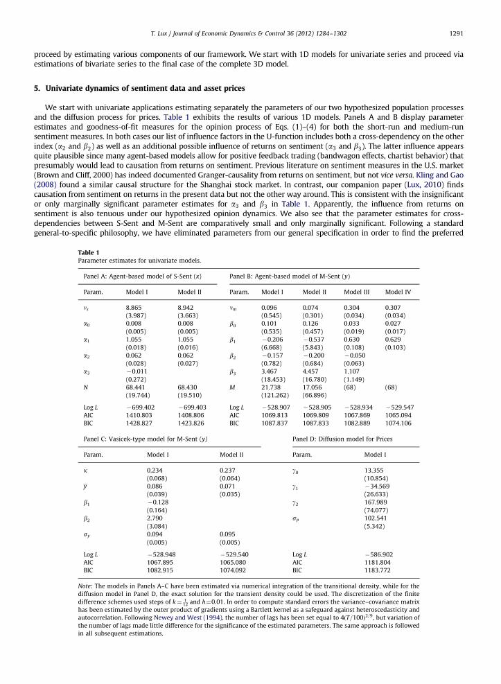
We start with univariate applications estimating separately the parameters of our two hypothesized population processesand the diffusion process for prices. Table 1 exhibits the results of various 1D models. Panels A and B display parameterestimates and goodness-of-fit measures for the opinion process of Eqs. (1)–(4) for both the short-run and medium-runsentiment measures. In both cases our list of influence factors in the U-function includes both a cross-dependency on the otherindex (a2 and b2) as well as an additional possible influence of returns on sentiment (a3 and b3). The latter influence appearsquite plausible since many agent-based models allow for positive feedback trading (bandwagon effects, chartist behavior) thatpresumably would lead to causation from returns on sentiment. Previous literature on sentiment measures in the U.S. market(Brown and Cliff, 2000) has indeed documented Granger-causality from returns on sentiment, but not vice versa. Kling and Gao(2008) found a similar causal structure for the Shanghai stock market. In contrast, our companion paper (Lux, 2010) findscausation from sentiment on returns in the present data but not the other way around. This is consistent with the insignificantor only marginally significant parameter estimates for a3 and b3 in Table 1. Apparently, the influence from returns onsentiment is also tenuous under our hypothesized opinion dynamics. We also see that the parameter estimates for cross-dependencies between S-Sent and M-Sent are comparatively small and only marginally significant. Following a standardgeneral-to-specific philosophy, we have eliminated parameters from our general specification in order to find the preferred

Table 1Parameter estimates for univariate models.

Panel A: Agent-based model of S-Sent (x) Panel B: Agent-based model of M-Sent (y)

Param. Model I Model II Param. Model I Model II Model III Model IV

ns 8.865 8.942 nm 0.096 0.074 0.304 0.307

(3.987) (3.663) (0.545) (0.301) (0.034) (0.034)

a0 0.008 0.008 b0 0.101 0.126 0.033 0.027

(0.005) (0.005) (0.535) (0.457) (0.019) (0.017)

a1 1.055 1.055 b1 �0.206 �0.537 0.630 0.629

(0.018) (0.016) (6.668) (5.843) (0.108) (0.103)

a2 0.062 0.062 b2 �0.157 �0.200 �0.050

(0.028) (0.027) (0.782) (0.684) (0.063)

a3 �0.011 b3 3.467 4.457 1.107

(0.272) (18.453) (16.780) (1.149)

N 68.441 68.430 M 21.738 17.056 (68) (68)

(19.744) (19.510) (121.262) (66.896)

Log L �699.402 �699.403 Log L �528.907 �528.905 �528.934 �529.547

AIC 1410.803 1408.806 AIC 1069.813 1069.809 1067.869 1065.094

BIC 1428.827 1423.826 BIC 1087.837 1087.833 1082.889 1074.106

Panel C: Vasicek-type model for M-Sent (y) Panel D: Diffusion model for Prices

Param. Model I Model II Param. Model I

k 0.234 0.237 g0 13.355

(0.068) (0.064) (10.854)

y 0.086 0.071 g1 �34.569

(0.039) (0.035) (26.633)

b1 �0.128 g2 167.989

(0.164) (74.077)

b2 2.790 sp 102.541

(3.084) (5.342)

sy 0.094 0.095

(0.005) (0.005)

Log L �528.948 �529.540 Log L �586.902

AIC 1067.895 1065.080 AIC 1181.804

BIC 1082.915 1074.092 BIC 1183.772

Note: The models in Panels A–C have been estimated via numerical integration of the transitional density, while for the

diffusion model in Panel D, the exact solution for the transient density could be used. The discretization of the finite

difference schemes used steps of k¼ 112 and h¼0.01. In order to compute standard errors the variance–covariance matrix

has been estimated by the outer product of gradients using a Bartlett kernel as a safeguard against heteroscedasticity and

autocorrelation. Following Newey and West (1994), the number of lags has been set equal to 4ðT=100Þ2=9, but variation of

the number of lags made little difference for the significance of the estimated parameters. The same approach is followed

in all subsequent estimations.


specification from our set-up. As a decision rule, we used the more parsimonious model, if the AIC information criterion votedin favor of it. Our tables also show how the more stringent BIC criterion changes with elimination of parameters, but selectionfollows the more lenient AIC to give the benefit of doubt to marginal entries. For S-Sent, the only determinant that could beeliminated in this way was the influence of returns, while dropping dependencies on M-Sent increased both AIC and BICslightly. Dropping the self-referential effect (i.e. setting a1 ¼ 0) led to a decrease of the log-likelihood from �699 to �1826which shows the importance of this factor. The final model version for S-Sent is thus Model II in Table 1A which only eliminatesthe hypothesized influence of returns on short-run sentiment.

Models I and II in Table 1, Panel B, show estimation results for medium-run sentiment with almost the same likelihoodobtained from different initial conditions. Furthermore, in contrast to the estimates for S-Sent, none of the parametersestimated for M-Sent under the two sets of initial conditions yielding Model I or Model II appears to be anywhere nearsignificance. Close inspection shows that the likelihood function is very flat, in particular, along the M axis. Since standarderrors are based on the curvature of the likelihood surface, the estimated standard errors will be extremely large. This situationindicates a multi-collinearity problem: the likelihood may be approximately linear in some parameters (inspection shows thatit is not exactly linear).

Further experimentation shows that practically any variation of M (we varied it from 1 to 200) leaves the likelihoodalmost unchanged. However, the number of agents, M, interacts strongly with the parameters nm and b1 that can changequite remarkably with different M’s. In the estimates of Model III, we have, therefore, fixed M¼68 (in line with theestimate for short-run sentiment) which leads to an increase of nm by three to four times and a change of the estimate of b1

from �0.21 of Model I to 0.630 (indicating a much higher intensity of interactions). Note that fixing M now leads tosignificant parameters for the key ingredients of the model (this actually happens for any M that we tried). It is, thus, a wayto overcome the near-collinearity problem. It is worthwhile to emphasize that (approximate) collinearity does notnecessarily imply misspecifiation of our model (cf. Kennedy, 2005, Chapter 11). Different specifications might just beobservationally nearly equivalent. This actually appears to be the case in our present framework. If interaction is weak, theopinion dynamics is close to a mean-reverting diffusion process in its time series properties. In this case, differentcombinations of the parameters nm, b1 and M lead to very similar aggregate dynamics, at least for small samples.10

Since it appears plausible that the number of agents is the same for both sentiment variables (as they come from thesame survey in which respondents are asked to provide both their forecast for the short and medium-term horizon), weproceed in the following mostly with restricted models obeying M¼N. As concerns the influence from returns onsentiment, the pertinent coefficient is again insignificant, but here in addition AIC and BIC improve if we drop the influenceof S-Sent so that the preferred model is one without exogenous factors (Model IV in Table 1B). Again, dropping theseentries and reestimating the parameters leads to minor changes only of the significant parameter estimates, while themaximized likelihood changes only very marginally.

A closer look at the remaining parameter estimates shows the following: short-run sentiment is characterized by aherding intensity a141, i.e. within the bi-modal regime. The frequency of agents’ revaluations of their mood (ns) is veryhigh—about 30 times as high as the corresponding parameter nm for medium-run sentiment. The impression from Fig. 1 isin harmony with these findings: short-run sentiment appears to change in a very rapid manner and seems to prefer moreextreme positive or negative values. There is also a small positive bias (a0) as well as a moderate reinforcement frommedium-run sentiment (a2). While these biases are small, they apparently add explanatory power as dropping themwould lead to a deterioration of at least the AIC criterion. Our ‘effective’ number of agents is estimated at about 68 forS-Sent, i.e. a model with 2N¼136 independent agents would get closest to the dynamic structure of the data.

As an alternative for our agent-based model, we have also estimated the Ornstein–Uhlenbeck type model of Eq. (5),cf. Panel C of Table 2. Although we could have estimated this model via the analytical solution of its transient density, weused the Crank–Nicolson discretization with the same grid as before for better comparability. As with the agent-basedmodel, the parameters for the influence of the short-run sentiment and returns are both insignificant. Medium-runsentiment, therefore, appears to evolve like an isolated variable without causal influence from the other components of ourdata set. This is actually again fully consistent with the results of the VAR analysis in our companion paper (Lux, 2010).Although the agent-based model and the OU diffusion process are not nested, it is tempting to compare their likelihoods.11

As we can see, the fit is practically the same which underlines our conjecture of the proximity of the agent-based model toa mean reverting diffusion for moderate levels of interaction.

It is interesting to remark that estimates of the Ornstein–Uhlenbeck process for S-Sent are clearly inferior in fit to theagent-based model so that we did not reproduce them here. We, thus, see that the practical equivalence between bothmodels only seems to hold for the uni-modal case. This is plausible as one can indeed show that the agent-based dynamicsconverges to an Ornstein–Uhlenbeck process in the limit of a large population (cf. Horst and Rothe, 2008; Lux, 2009a).However, the Ornstein–Uhlenbeck process could serve as only a good approximation for the fluctuations around one modewithin its basin of attraction. It is, therefore, plausible that the Ornstein–Uhlenbeck process provides a close substitute forthe agent-based model in the uni-model case, but not so in the bi-model case.

10 We actually also found the same problem of approximate collinearity in Monte Carlo experiments with data generated from our population

process for cases of weak interaction.11 Since we have used exactly the same grid in (y,t) space in both estimation algorithms, the likelihoods are comparable in the sense that they result

from the assignment of probability mass to the same cells (intervals) on the base of two different estimated models.


We finally turn to estimates for the price dynamics, Eq. (6). In the complete Model I we find an insignificant parameterfor short-run sentiment, but a strongly significant positive influence of medium-run sentiment. However, only the BICcriterion votes for chipping this parameter, while the AIC criterion deteriorates when eliminating this factor.

Table 2Parameter estimates for bi-variate models.

Panel A: Interaction of S-Sent and M-Sent

Param. Model I Model II Model III Model IV

ns 8.702 8.994 8.837 9.160

(4.722) (4.659) (4.728) (4.670)

a0 0.008 0.008 0.008 0.008

(0.006) (0.006) (0.006) (0.006)

a1 1.059 1.057 1.059 1.058

(0.020) (0.018) (0.020) (0.018)

a2 0.056 0.056 0.055 0.055

(0.032) (0.031) (0.031) (0.030)

a3 �0.045 �0.045

(0.319) (0.315)

N 66.251 66.108 67.265 67.216

(22.546) (22.339) (22.613) (22.373)

um 0.259 0.258

(0.102) (0.101)

b0 0.072 0.073

(0.038) (0.036)

b1 0.642 0.642

(0.176) (0.165)

b2 �0.262 �0.265

(0.136) (0.135)

b3 2.836 2.867

(1.429) (1.444)

M M¼N M¼N

k 0.194 0.194

(0.073) (0.069)

y 0.192 0.192

(0.070) (0.070)

b1 �0.690 �0.693

(0.356) (0.356)

b2 7.441 7.453

(3.904) (3.770)

sy 0.088 0.088

(0.007) (0.007)

lkl �1019.908 �1019.202 �1019.817 �1019.839

AIC 2061.816 2059.857 2061.635 2059.678

BIC 2094.859 2089.896 2094.678 2089.717

Panel B: S-Sent and Prices

Param. Model I Model II

ns 8.438 8.934

(3.874) (3.947)

a0 0.013 0.013

(0.008) (0.007)

a1 1.058 1.056

(0.024) (0.018)

a3 �0.099

(0.293)

N 64.552 64.284

(21.072) (20.338)

g0 �5.617

(17.225)

g1 144.041 134.203

(67.947) (53.939)

sp 95.657 96.044

(5.626) (5.563)

lkl �911.725 �911.991

AIC 1839.449 1835.981

BIC 1836.481 1854.005

Table 2 (continued )

Panel C: M-Sent and Prices


nm 0.313 0.313

(0.042) (0.042)

b0 0.026 0.028

(0.017) (0.017)

b1 0.633 0.633

(0.103) (0.099)

b3 0.394

(0.777)

M (68) (68)

k 0.238 0.239

(0.069) (0.067)

y 0.069 0.073

(0.038) (0.036)

b3 0.996

(2.048)

sy 0.095 0.096

(0.006) (0.006)

g0 26.195 26.270 21.102 26.308

(12.183) (10.931) (12.483) (10.920)

g2 3.593 70.103

(104.473) (113.011)

sp 105.568 105.647 105.235 105.626

(5.272) (5.120) (5.244) (5.131)

lkl �749.870 �750.104 �749.235 �749.938

AIC 1513.739 1510.209 1512.470 1509.877

BIC 1534.767 1525.228 1533.498 1524.896

Note: The models in Panels A to C have been estimated via numerical integration of the transitional

density using the ADI (alternative direction implicit) algorithm detailed in the Appendix. The discretiza-

tion of the finite difference schemes used steps of k¼ 112 (for time), and h¼0.02 (for S-Sent and M-Sent). In

Panels B and C, the discretization of the second space dimension (prices) is chosen in a way to generate

the same number of grid points as in the x or y dimension, i.e. Nx ¼Ny ¼Np ¼ 100. This amounts to

roughly 43 basis points of the DAX index.


6. Bivariate dynamics

We proceed by estimating bivariate models for each pair of our three variables, x, y and p.Our interest is now to explore the robustness of our previous 1D estimates. This means (i) robustness with respect to

inclusion of a second simultaneous dynamic process and (ii) robustness with respect to different discretization schemes.Panel A of Table 2 exhibits parameter estimates for a bi-variate simultaneous opinion dynamics for the short-run andmedium-run sentiment indices. Model I indicates the unrestricted model, whereas Model II stands for the reduced modelwith which we end up after a sequence of estimates of restricted models. As we encountered again the problem of a veryflat surface of the likelihood function in the M direction, we only give results with the restriction M¼N imposed. Again,with M endogenous, very different parameters can be obtained with practically equal likelihood. Experimenting with thestarting values, we found that the parameters for the short-run sentiment dynamics were pretty unaffected while those forthe medium-term components showed more variations. This is completely in line with the behavior of the pertinent 1Dmodels. Apparently, component-wise estimation and simultaneous estimation of both dynamic processes leads to prettymuch the same outcome. Fixing N¼M allows us to obtain meaningful standard errors for all parameters. These indicatethat almost all parameters are significant although the significance of the biases (a0,b0) and cross-dependencies (a2,b2) ismore or less marginal. From the coefficients for past returns (a3,b3) only the later survives the model selection procedure.The relatively weak interaction between S-Sent and M-Sent is again in line with VAR parameter estimates in ourcompanion paper.

Fig. 2 shows the stationary distribution of our estimated stochastic opinion dynamics. Since an analytical solution is notavailable for our highly nonlinear bi-variate Fokker–Planck equation, we have simply integrated the transitional densityover a very long time horizon until it converged to a stationary distribution in order to obtain Fig. 2 upper panel. As can beseen, we find a distribution that is at the margin between bi-modality and pronounced skewness. While probability massis concentrated around zero along the y axis, the stationary distribution has a maximum at about 0.6 for S-Sent togetherwith non-negligible probabilities along the whole range between about �0.7 and þ0.7. A kernel density estimate of theempirical in-sample distribution shows a close coincidence of the non-parametric kernel estimate and the limitingdistribution of our parametric model.

Fig. 2. The upper panel exhibits the limiting distribution of the joint opinion dynamics for S-Sent and M-Sent (Model II of Table 2, Panel A, with the level

of returns set equal to zero). Note that a plot of the limiting distribution of Model IV (opinion dynamics for S-Sent and OU process for M-Sent is

undistinguishable from the one displayed here). The lower panel shows a bivariate kernel density of the in-sample record using a Gaussian kernel with

100 bins in each direction and a bandwidth of 0.1.


Because of the collinearity in the y component, we also combined the opinion dynamics in x with the OU type diffusionfor y (Model III in Panel A). The pertinent parameter estimates are all significant. While k and sy correspond closely to theircounterparts in the univariate estimation exercises of Table 1, y, b1 and b2 show somewhat more variation. Again, only a3

from the opinion dynamics governing S-Sent seems dispensable under the AIC selection rule. Most interestingly, however,the likelihood of this alternative model is practically the same as the one for the simultaneous opinion dynamics of ModelsI and II. The stationary distribution from Model III is, in fact, entirely undistinguishable from the one shown in Fig. 2. Again,this conformity underlines our impression that a population process could be largely equivalent to a simple diffusionmodel in the presence of relatively weak interaction.

Panels B and C provide parameter estimates for joint bi-variate dynamic processes of each one of our sentiment indicesand the share index DAX. For S-Sent, we see that the parameters of the opinion process remain unchanged, but thesentiment-based component (g1) of the price dynamics seems highly significant which is in contrast to the previous resultof the univariate diffusion for prices. For M-Sent, we have again estimated an opinion formation model with M fixed at 68 and


the OU diffusion. Parameters are close to previous ones with again almost the same quality of the fit, but here we encounter aninsignificant parameter for the influence from medium-run sentiment on prices (g2) which is in contrast to the results obtainedfor the 1D price dynamics of Section 5. In the OU approach, the model selection exercise arrives at a model that has the samestructure like the agent-based model dispensing with both the influence of M-Sent on returns as well as with the effect in theopposite direction.

7. The complete 3D models

We finally turn to parameter estimates from joint models of all three variables: x, y and p. Unfortunately, with currentcomputational resources, the maximum likelihood estimation in the 3D case approaches the limit of feasible scenarios.Using one processor, one full estimation takes a couple of days while the time required can be reduced almostproportionally to the number of cores with a parallel computing framework.

Table 3 shows results for two models again using both a second population process or an OU diffusion for medium-runsentiment. Again, we have not been able to obtain meaningful standard errors in variants of our model (not displayed)

Table 3Parameter estimates for tri-variate models.


ns 8.222 8.182 8.413 8.307

(4.012) (3.992) (4.032) (3.992)

a0 0.008 0.008 0.008 0.008

(0.008) (0.006) (0.007) (0.006)

a1 1.054 1.055 1.055 1.055

(0.021) (0.020) (0.020) (0.019)

a2 0.069 0.070 0.068 0.069

(0.041) (0.035) (0.040) (0.034)

N 63.545 63.965 64.954 64.892

(23.996) (22.968) (24.145) (23.077)

nm 0.227 0.230

(0.107) (0.102)

b0 0.082 0.078

(0.041) (0.039)

b1 0.652 0.660

(0.190) (0.179)

b2 �0.315 �0.299

(0.169) (0.161)

b3 3.041 2.944

(1.643) (1.563)

M M¼N M¼N

k 0.165 0.162

(0.076) (0.074)

y 0.225 0.220

(0.097) (0.091)

b1 �0.860 �0.840

(0.498) (0.490)

b2 8.254 8.275

(4.697) (4.742)

sy 0.085 0.085

(0.009) (0.008)

g0 �13.164 – �13.149 –

(18.844) (18.804)

g1 156.547 145.180 156.605 144.989

(62.986) (53.001) (63.078) (52.931)

g2 77.515 – 77.558 –

(122.597) (122.929)

sp 89.261 90.330 89.262 90.343

(7.942) (7.382) (8.006) (7.418)

lkl �1591.926 �1593.078 �1591.825 �1592.977

AIC 3211.852 3210.155 3211.649 3209.953

BIC 3253.907 3246.203 3253.704 3246.000

Note: All models have been estimated via numerical integration of the transitional density using a tri-variate ADI

(alternative direction implicit) algorithm as detailed in the Appendix. The discretization of the finite difference schemes

used steps of k¼ 18 (for time), and h¼0.02 (for S-Sent and M-Sent). The discretization of the second space dimension

(prices) is chosen in a way to generate the same number of grid points as in the x or y dimension, i.e. Nx ¼Ny ¼Np ¼ 100.

This amounts to roughly 43 basis points of the DAX index.


with different ‘effective’ numbers of agents for the two population processes governing S-Sent and M-Sent. Fixing M¼N apriori, meaningful standard errors are obtained throughout in line with previous estimates for the 1D and 2D cases. Withthe Ornstein–Uhlenbeck process replacing the agent-based opinion dynamics of M-Sent (Models III and IV), parameterestimates of the remaining dynamic components and maximized likelihood are in line with those of models I and II. Whileall parameters of the opinion dynamics are quite homogenous across our various models, the influence from sentiment onprices appears less robust. In models I and III of Table 3, we find significant influence from S-Sent, but insignificant (or onlymarginally significant) influence from M-Sent on prices. While this appears in harmony with the bivariate models ofTable 2, it is in contrast to the univariate diffusion estimated in Panel C of Table 1. It is also in contrast to the results of ourprevious VAR estimates (Lux, 2010) indicating Granger causality from M-Sent on prices, but not so from S-Sent. In order toassess the contribution of g1 to the fit of the models, we also estimated restricted versions of the 3D framework without aninfluence from S-Sent on prices. As it turned out this leaves all other parameters more or less unchanged but decreases thelikelihood considerably. So, in principle, there seems no reason to skip this term.

We have also conducted an out-of-sample forecasting exercise using the various estimated 3D models (as well as thesimpler 1D and 2D models). Table 4 exhibits as an example root-mean squared errors relative to the benchmark of a randomwalk with drift for the agent-based Model II of Table 3. Out-of-sample returns comprise 188 weekly entries and forecastinghorizons of one week up to eight weeks are investigated. Results are depicted for single-week returns as well as for cumulativereturns over the pertinent horizon. Because of the bi-modality of our estimated models (in the S-Sent dimension) we usedifferent predictors: Besides the mean, we also use the nearest mode of two in the bi-modal case or the global maximum, i.e.the coordinates with the highest probability mass. This approach follows Creedy et al. (1996) who use a bi-modal error term inan otherwise linear monetary model of the exchange rate. The ‘nearest’ and ‘global’ forecast conventions are justified bythe observation that the mean might actually be a very unlikely realization in a bi-modal stochastic process. Because of thepersistence of the process, there could be a certain chance that the realization in the near future might remain close to thepreviously dominant mode (which justifies the ‘nearest’ convention). On the other hand, one might use the global maximum ofthe predictive distribution as the most probable single value which also might be quite remote from the mean.

While our results in Table 4 show sometimes a slight improvement over the random walk forecasts, the Diebold–Mariano statistics for better predictive performance are all insignificant at all time horizons, and we also do not find muchdifference between the three different predictors we have chosen. The same applies to models that use an Ornstein–Uhlenbeck process for M-Sent as well as to forecasts from simpler 1D or 2D models. We have also performed out-of-sample tests of predictability based upon the comparison of the predictive densities (i.e. using the sum of likelihood ratiosfor different models over the out-of-sample entries, cf. Mitchell and Hall, 2005). As it turned out, we could not reject thehypothesis of equal performance of any of the estimated models and the random walk in price forecasts at the 95significance level. However, when applying this method to the other quantities involved (S-Sent and M-Sent), we foundthat the agent-based models as well as (in the case of M-Sent) the Ornstein–Uhlenbeck model to dominate over randomforecasts from a Normal distribution with mean and variance equal to the historical (in-sample) mean and variance at the99% significance level throughout (i.e. for all specifications). No wonder after the previous results, we found no significantdifference in the performance of the agent-based model vis-�a-vis the Ornstein–Uhlenbeck model for M-Sent. In contrast,for S-Sent the agent-based model beats the Ornstein–Uhlenbeck model at the 95% significance level under the comparisonof predictive densities. This shows that the bi-modality of the estimated process is an indispensable feature of thedynamics of this component of our bivariate data set that cannot be captured by a simple linear process. This is differentfor M-Sent where the agent-based model and the OU process have essentially the same fit both in-sample and out-of-sample. Overall, the in-sample estimates for the sentiment dynamics do, thus, also perform well in out-of-sampleforecasting of the evolution of sentiment itself. However, the link between sentiment and returns is apparently too

Table 4RMSEs of out-of-sample forecasts from tri-variate Model II.

Horizon 1-Period returns Multiperiod returns

Near Global Mean Near Global Mean

Forecasts from Model II

1 1.015 1.021 1.013 1.015 1.021 1.013

2 1.046 1.042 0.988 1.062 1.028 1.002

3 1.050 1.060 1.026 1.082 1.041 1.024

4 0.981 1.052 1.003 1.090 1.102 1.027

5 1.018 1.030 0.999 1.080 1.100 1.024

6 0.998 0.991 0.982 1.066 1.074 1.019

7 1.027 1.019 1.024 1.085 1.075 1.038

8 0.996 1.002 0.989 1.077 1.069 1.035

Note: The table shows relative MSEs of the forecasts under the pertinent convention (i.e. original MSE divided by that of

Brownian motion with drift). Diebold–Mariano statistics for better predictive ability are all insignificant at standard

confidence levels.


tenuous for successful forecasting on the base of the present approach. Note that in Lux (2010) VAR models with constantcoefficients were also not successful in forecasting returns from their joint dynamics with sentiment. It was only withiteratively updated estimates and updating of the selection of an appropriate subset VAR model that some improvementsover the random walk could be obtained.

8. Conclusions

Given the long lasting interest in sentiment data in financial economics, it might come as a surprise that there is hardlyany empirical work estimating and testing behavioral models for such data. Of course, under an efficient marketperspective, such data would represent a relatively unimportant noise component. However, evidence exists for a certainimpact of sentiment on prices. While for U.S. data, Granger causality in the short-run seems to run from returns tosentiment (Brown and Cliff, 2004), our German data indicate a causal relationship in the opposite direction (Lux, 2010).Even for the U.S., however, some predictive power of sentiment has been found for longer horizons (Brown and Cliff, 2005).

The significant influence of sentiment on returns in the German data motivated us to adopt a behavioral, agent-basedframework for the dynamics of short- and medium-run sentiment. In order to estimate the parameters of such models, wecould take stock of an approach proposed in Lux (2009a) using a numerical maximum likelihood procedure. In terms ofmethodology, the contribution of this paper is the extension of this estimation technique to higher dimensions. MonteCarlo simulations in Lux (2009a) showed that this method performed well even in relatively small samples like the presentone. Choosing appropriate methods from the large range of finite difference approximations for partial differentialequations allowed an extension of the univariate approach to 2D and 3D.

Materially, we found evidence for strong social interaction in short-term sentiment and only moderate social influences inmedium-run sentiment. With moderate interaction, estimation of the agent-based model appears somewhat cumbersomebecause of almost collinear behavior of some parameters. As we have seen, in this case, a more parsimonious Ornstein–Uhlenbeck process provides practically the same fit to the data. One could, therefore, use a simple macroscopic equationinstead of the full microscopic Markov process. We believe that results like this one are important in that they provide anindication of the necessary degree of complexity of behavioral models in different scenarios (an issue very much neglected ineconomics where theoretical models are mostly either based on the assumption of a representative agent or an infinitepopulation).

This also means that there is not necessarily a conflict between agent-based modeling and modelling of aggregate datavia structural equations. On the contrary, combining an analytical approach for the derivation of appropriate approxima-tions to the agent-based stochastic Markov process with an approach for empirical estimation of the later, we were able toshow that under certain conditions two very different functional specifications can yield practically undistinguishableresults. However, this congruence crucially depends on the parameter values and might break down (as it does here for S-Sent) if other parameters lead to another type of system behavior.

Overall, most of our results were in nice coincidence with the previous VAR results of Lux (2010). The social dynamicsestimated for S-Sent and M-Sent, therefore, seems a potential candidate for a data generating process of our sample. Whileour forecasting exercise turned out disappointing results for price forecasts, this might be due to potential non-stationarityof the returns process during our out-of-sample period that coincides with the last three years of financial turmoil. Due tothe computational demands of the present approach, all forecasts were conducted on the base of the fixed parameterestimates from the in-sample period. Note that more successful forecasts from VAR models were based on iterativeupdating of both paramaters and the selection for the appropriate VAR subset model, and did indeed find quite somevariation of the influence of S-Sent vs M-Sent on returns throughout pretty much the same out-of-sample period. Wemight hope that moving towards iterative updating of parameters for the present approach might also help to capturebetter the subtleties of joint causation from various sentiment indicators on returns. Current attempts at developing a fullyparallel algorithm for the present approach will allow us to revisit the forecasting capacity of the opinion models with aniterative approach in the near future.

We believe that the present paper and its predecessor (Lux, 2009a) could provide an avenue to empirical estimation of abroad range of agent-based models. While we noted that we reached the limits of current computational power at our 3Dapplications, we also note that we have only used a small range of numerical schemes so far. Methods using adaptiveadjustment of meshes or refined methods for parallelization of tasks might allow us to dramatically reduce computationtime in future applications. Further research in this direction should be of high priority.

Acknowledgments

Helpful comments by Martin Burger, Hans Dewachter, Guido Germano, Enrico Scalas, David Veredas and threeanonymous referees are gratefully acknowledged. The author also wishes to thank the Volkswagen Foundation for itsfinancial support of the research reported in this paper.


Appendix A. Finite difference schemes for the Fokker–Planck equation

(1) FP Equation in1D: In the case of a univariate series, the FP equation for the density qðx; tÞ of a variable xt reads as

@qðx; tÞ

@t¼

@

@xðAðx,yÞqðxÞÞþ

@2

@x2ðBðx,yÞqðxÞÞ

with y the set of parameters we wish to estimate.Defining the flux F(x), the FP equation can be more compactly written as

@qðx; tÞ

@t¼@Fðx,tÞ

@xðA:1Þ

with

FðxÞ ¼ BðxÞ@qðx; tÞ

@xþ AðxÞþ

@BðxÞ

@x

� �qðx; tÞ:

Denote by Qij a discrete evaluation of the transient density at space and time coordinates ðxj,tiÞ, with grid points

xj ¼ x0þ jh; j¼ 0;1, . . .Nx and ti ¼ ik with i¼ 0, . . . ,Nt . Different possibilities exist to discretize Eq. (A.1). The Crank–Nicolsonscheme approximates the flux at intermediate points ðiþ1

2Þk which can be interpreted as an arithmetic average between aforward (explicit) and backward (implicit) approximation. We, thus, obtain the following finite difference approximationto (A.1)

Qiþ1j �Qi

j

k¼

1

h

Fiþ1jþ1=2þFi

jþ1=2

2�

Fiþ1j�1=2þFi

j�1=2

2

!: ðA:2Þ

Note that on the right-hand side of (A.2), the discrete approximation of the derivative with respect to x has also usedthe central difference over the cell mid points x0þðj�

12Þh and x0þðjþ

12Þh. Since the discretization of the flux implies

Fij ¼ BðxjÞ

Qijþ1=2�Qi

j�1=2

hþðAðxjÞQ

ijþB0ðxjÞQ

ijÞ ðA:3Þ

we arrive at

Qiþ1j �Qi

j

k¼

1

2hBjþ1=2

Qiþ1jþ1�Qiþ1

j

hþðAjþ1=2þB0jþ1=2ÞQ

iþ1jþ1=2

(þBjþ1=2

Qijþ1�Qi

j


ijþ1=2

�Bj�1=2

Qiþ1j �Qiþ1

j�1

h�ðAj�1=2þB0j�1=2ÞQ

iþ1j�1=2�Bj�1=2

Qij�Qi

j�1


ij�1=2

): ðA:4Þ

Using averages Qjþ1=2 �12 ðQ

ijþ1þQi

jÞ as well as another finite difference approximation to B0 (i.e. B0jþ1=2 ¼ ðBjþ1�BjÞ=h)we can rearrange the system into the form:

ajQiþ1j�1 þbjQ

iþ1j þcjQ

iþ1jþ1 ¼ djQ

ij�1þejQ

ijþ f jQ

ijþ1: ðA:5Þ

Since this derivation applies to all values j¼ 0;1, . . . ,Nx on our grid, we end up with a computationally convenient tri-diagonal system of equations that approximates the continuous-time dynamics of the transient density qðx; tÞ

VQ iþ1¼ ri ðA:6Þ

with

V¼

b0 c0 0 . . .

a1 b1 c1 . . .

. . . aNx�1 bNx�1 cNx�1

. . . 0 aNxbNx

26666664

37777775

Q iþ1¼ ðQiþ1

0 ,Qiþ11 , . . . ,Qiþ1

NxÞ0

and

ri ¼ ðe0Qi0þ f 0Qi

1,d1Qi0þe1Qi

1þ f 1Qi2, . . . ,dNx

QiNx�1þeNx

QiNxÞ0:

Note that the definition of our grid from x0 to x0þ j � Nx implies that at the edges of our system of equations, coefficientsoutside the ðNxþ1Þ � ðNxþ1Þ matrix V are indeed equal to zero (e.g. for j¼0, the term a0Qi

�1 vanishes for all i). While thiswould impose a certain arbitrariness in truncation of the underlying state space in certain applications (e.g. when evaluatingthe Black–Scholes partial differential equation), in our case of a finite state space for the sentiment data this truncation wouldbe quite natural. In order to conserve overall probability mass (or number of particles) additional ‘no-flux’ conditions have to be


imposed. Going back to (A.1), these can be simply defined as

Fi�1=2 ¼ Fi

Nxþ1=2 ¼ 0 8i:

This keeps all the mass within the confines of the range ½x0,x0þhNx�. Keeping track of these boundary conditions, we obtainslightly different definitions of the coefficients aj,bj,cj at j¼0 and j¼Nx at the edges of the matrix V. The Crank–Nicolsonscheme is known to be of accuracy Oðk2

ÞþOðh2Þ at the grid points.

(2) FP Equation in2D: Note that for bivariate and tri-variate systems, the Fokker–Planck Eq. (7) has drift and diffusioncomponents consisting of the pertinent functions of the various models as we have presented them above. To write downthe multi-variate Fokker–Planck equation is therefore, straightforward.

While it is feasible to apply the Crank–Nicolson scheme to higher dimensions, it is problematic from the computationalpoint of view. The reason is that the resulting system of equations can not be cast into the form of sparse, tri-diagonalsystems of equations anymore. A popular alternative that preserves the tri-diagonal forms for higher dimensions is theclass of alternative direction implicit schemes (ADI schemes). In our numerical approximation of bivariate and tri-variate FPequation, we apply two particular variants from the rich class of ADI schemes.

To set the stage for the 2D and 3D applications, let us first explain the implicit scheme in 1D. This scheme is obtained byapproximating the flux in Eq. (A.1) at points ðiþ1Þk so that instead of (A.2) we arrive at

Qiþ1j �Qi

j

k¼

1

hðFiþ1

jþ1=2�Fiþ1j�1=2Þ:

Inserting (A.3) we derive:

Qiþ1j �Qi

j

k¼

1

hBjþ1=2

Qiþ1jþ1�Qiþ1

j


iþ1jþ1=2

(�Bj�1=2

Qiþ1j �Qiþ1

j�1


i�1j�1=2

):

Rearranging the components of this system, we arrive at a linear system of equations similar to the one obtained for theCrank–Nicolson scheme:

ajQiþ1j�1 þbjQ

iþ1j þcjQ

iþ1jþ1 ¼ Qi

j:

Instead of (A.6) we now have a tri-diagonal system:

VQ iþ1¼Q i

with appropriate boundary conditions. Note that in 1D the simplification of the expression on the right-hand side isnegligible in terms of computational demand. Since the computational demands of the (fully) implicit and Crank–Nicolsonscheme are practically the same, and the implicit method is of first-order accuracy only, we would typically prefer Crank–Nicolson (so that the later was our natural choice for univariate problems).

In 2D computational demands make a difference. Both a direct adaptation of the fully implicit and Crank–Nicolsonschemes would lead to broadly banded matrix equations that lack the tri-diagonal charm of those derived in 1D. A way topreserve this convenient form is to use an indirect scheme in an alternating way first performing a half (or auxiliary) stepinto one space dimension and subsequently another half (auxiliary) step into the second space dimension. To provide moredetails, let us denote the space variables as x1 and x2 with grids: x1,j ¼ x1;0þ j � h1, j¼ 0;1, . . . ,Nx1

and x2,l ¼ x2;0þ l � h2,l¼ 0;1, . . . ,Nx2

.The bivariate FP equation can be rewritten using the concept of fluxes in both the x1 and x2 direction as

@qðx1,x2,tÞ

@t¼@F1ðx1,x2,tÞ

@x1þ@F2ðx1,x2,tÞ

@x2

with

Frðx1,x2; tÞ ¼X

s

Brsðx1,x2,tÞ@qðx1,x2,tÞ

@xsþðArðx1,x2Þþ

Xs

@Brsðx1,x2Þ

@xsÞqðx1,x2; tÞ:

As it turns out, inclusion of the off-diagonal terms, B12ð�Þ and B21ð�Þ is potentially problematic for a number of reasons:First, in terms of our bivariate opinion process, we would have to make explicit the dependence between respondents’opinion on the short- and medium-run. While it is perfectly reasonable to assume some dependency, to come up with aformal framework for this dependent opinion formation would be demanding. We are, therefore, tempted to maintain theassumption of independent Markov processes as data-generating processes for S-Sent and M-Sent. By this assumption,Brs ¼ 0 for ras follows as a consequence of the model set-up. In addition, setting the off-diagonal terms of the diffusionmatrix equal to zero is computationally convenient as certain results on the accuracy of ADI schemes only apply in theabsence of cross-derivatives and a strong off-diagonal influence could also jeopardize positivity of our solutions.

Our method of choice for the 2D case without cross-derivatives is the ADI scheme proposed by Peaceman and Rachford(cf. Strikwerda, Chapter 7). Denoting the finite difference approximation of the transient density in 2D by Qi

j,l, i.e. qðx1,x2; tÞ

evaluated at x1,j, x2,l and ti, one first evaluates the derivative with respect to x1 implicitly and that with respect to x2


explicitly using a time step k=2:

Qiþ1=2j,l �Qi

j,l

k=2¼

1

h1ðFiþ1=2

1,jþ1=2,l�Fiþ1=21,j�1=2,lÞþ

1

h2ðFi

2,j,lþ1=2�Fi2,j,l�1=2Þ:

For the next half step, the order is changed leading to:

Qiþ1j,l �Qiþ1=2

j,l

k=2¼

1

h1ðFiþ1=2

1,jþ1=2,l�Fiþ1=21,j�1=2,lÞþ

1

h2ðFiþ1

2,j,lþ1=2�Fiþ12,j,l�1=2Þ:

As can easily be seen, both half-steps lead to a tri-diagonal system of equations with the explicit expressions all enteringinto the term on the right-hand side. Boundary conditions are easily imposed by setting Fi

1,�1=2,l ¼ Fi1,Nx1

þ1=2,l ¼ 0 for all i,l andFi

2,j,�1=2 ¼ Fi2,j,Nx2

þ1=2 ¼ 0 for all i,j. Like the implicit scheme in 1D, the Peaceman–Rachford scheme is unconditionally stable. Itis also second-order accurate in Dt, Dx1 and Dx2 (although the 1D implicit scheme is only of first-order accuracy) as long as thecross-derivatives are all equal to zero (Strikwerda, c.7).

(3) FP Equation in3D: A generalization of the Peaceman–Rachford scheme to three space dimensions (xi, i¼1, 2, 3) canbe found in Morton and Mayers (1994, Chapter 3).

With our FP equation expressed in fluxes:

@qðx; tÞ

@t¼X

r

@Frðx : tÞ

@xr, r¼ 1;2,3

and the approximation to the transient density at ðti,x1,j,x2,l,x3,mÞ denoted by Qij,l,m, this scheme amounts to the following

sequence of systems of equations:

Qiþn

j,l,m�Qij,l,m

k¼

1

h1ðFiþn

1,jþ1=2,l,m�Fiþn

1,j�1=2,l,mÞþ1

h2ðFi

2,j,lþ1=2,m�Fi2,j,l�1=2,mÞþ

1

h3ðFi

3,j,l,mþ1=2�Fi3,j,l,m�1=2Þ,

Qiþnn

j,l,m �Qiþn

j,l,m

k¼

1

h2ðFiþnn

2,j,lþ1=2,m�Fiþnn

2,j,l�1=2,mÞ�1

h2ðFi

2,j,lþ1=2,m�Fi2,j,l�1=2,mÞ,

Qiþ1j,l,m�Qiþnn

j,l,m

k¼

1

h3ðFiþ1

3,j,l,mþ1=2�Fiþ13,j,l,m�1=2Þ�

1

h3ðFi

3,j,l,mþ1=2�Fi3,j,l,m�1=2Þ:

Here, the intermediate steps iþn and iþnn are better interpreted as auxiliary rather than fractional steps since thesecond and third systems of equations is more of an error-correction form. Unfortunately, Morton and Mayers do notmention the order of accuracy of this scheme. This approach has been used to solve three-dimensional heat conductionequations. Within this simpler setting, it has been demonstrated to be unconditionally stable and of first-order accuracy inDt (Marschak, 1990, section 28). Most importantly for our purposes it seems to be the method with least computationaldemands among the many variants of ADI and related finite difference methods for higher dimensions.

References

Ait-Sahalia, Y., 1996. Testing continuous-time models of the spot interest rate. Review of Financial Studies 9 (2), 385–426.Alfarano, S., Lux, T., Wagner, F., 2008. Time-variation of higher moments in financial markets with heterogeneous agents: an analytical approach. Journal

of Economic Dynamics & Control 32, 101–136.Amilon, H., 2008. Estimation of an adaptive stock market model with heterogeneous agents. Journal of Empirical Finance 15, 342–362.Boswijk, P., Hommes, C., Manzan, S., 2007. Behavioral heterogeneity in stock prices. Journal of Economic Dynamics & Control 31, 1938–1970.Branch, W., 2004. The theory of rationally heterogeneous expectations: evidence from survey data on inflation expectations. Economic Journal 114,

592–621.Brown, G., Cliff, M., 2004. Investor sentiment and the near-term stock market. Journal of Empirical Finance 11, 1–27.Brown, G., Cliff, M., 2005. Investor sentiment and asset valuation. Journal of Business 78, 405–440.Creedy, J., Lye, J., Martin, V., 1996. A non-linear model of the real US/UK exchange rate. Journal of Applied Econometrics 11, 669–686.Ethier, S., Kurtz, T., 1986. Markov Processes. New York, Wiley.Franke, R., 2009. Applying the method of simulated moments to estimate a small agent-based asset pricing model. Journal of Empirical Finance 16,

804–815.Franke, R., 2008. A microfounded herding model and its estimation on German survey expectations. Intervention, European Journal of Economics and

Economic Policies 5, 301–328.Gardiner, C.W., 2004. Handbook of Stochastic Methods, 3rd ed. Springer, Berlin.Goldbaum, D., Mizrach, B., 2008. Estimating the intensity of choice in a dynamic mutual fund allocation decision. Journal of Economic Dynamics & Control

32, 3866–3876.Horst, U., Rothe, C., 2008. Queuing, social interactions, and the microstructure of financial markets. Macroeconomic Dynamics 12, 211–233.Hurn, S., Jeisman, J.I., Lindsay, K., 2007. Seeing the wood for the trees: a critical evaluation of methods to estimate the parameters of stochastic differential

equations. Journal of Financial Econometrics 5, 390–455.Iori, G., 2002. A micro-simulation of traders’ activity in the stock market: the role of heterogeneity of agents’ interactions and trade-friction. Journal of

Economic Behavior and Organisation 49, 269–285.Kennedy, P., 2005. A Guide to Econometrics, 5th ed. MIT-Press, Cambridge.Klein, A., Urbig, D., Kirn, S., 2008. Who Drives the Market? Estimating a Heterogeneous Agent-based Financial Market Model Using a Neural Network

Approach. Manuscript, University of Hohenheim.


Kirman, A., 1993. Ants, rationality, and recruitment. Quarterly Journal of Economics 108 (1), 137–156.Kling, G., Gao, L., 2008. Chinese institutional investors’ sentiment. International Financial Markets, Institutions and Money 18, 374–387.Lux, T., 1995. Herd behavior, bubbles and crashes. Economic Journal 105, 881–896.Lux, T., 1998. The socio-economic dynamics of speculative markets: interacting agents, chaos, and the fat tails of return distributions. Journal of Economic

Behavior and Organization 33, 143–165.Lux, T., Marchesi, M., 1999. Scaling and criticality in a stochastic multi-agent-model of a financial market. Nature 397, 498–500.Lux, T., Marchesi, M., 2000. Volatility clustering in financial markets: a microsimulation of interacting agents. International Journal of Theoretical and

Applied Finance 3, 675–702.Lux, T., 2009a. Rational forecasts or social opinion dynamics? Identification of interaction effects in a business climate survey. Journal of Economic

Behavior and Organization 72, 638–655.Lux, T., 2009b. Stochastic behavioral asset pricing models and the stylized facts. In: Hens, T., Schenk-Hopp, K. (Eds.), Handbook of Financial Markets:

Dynamics and Evolution. North-Holland (Chapter 3).Lux, T., 2010. Sentiment dynamics and stock returns: the case of the German stock market. Empirical Economics 41, 663–679.Marschak, G., 1990. Splitting and alternating direction methods. In: Ciarlet, P., Lions, J. (Eds.), Handbook of Numerical Analysis, vol. 1. Amsterdam, North-

Holland, pp. 199–462.Mitchell, J., Hall, S.G., 2005. Evaluating, comparing, and combining density forecasts using the KLIC with an application to the Bank of England and NIESR

‘Fan’ charts of inflation. Oxford Bulletin of Economics and Statistics 67 (Supplement), 995–1033.Morton, K., Mayers, D., 1994. Numerical Solution of Partial Differential Equations. University Press, Cambridge.Newey, W., West, K., 1994. Automatic lag selection in covariance matrix estimation. Review of Economic Studies 61, 631–653.Pape, B., 2007. Asset allocation and multivariate position based trading. Journal of Economic Interaction and Coordination 2, 163–193.Poulsen, R., 1999. Approximate Maximum Likelihood Estimation of Discretely Observed Diffusion Processes. Manuscript, University of Aarhus.Risken, H., 1989. The Fokker–Planck Equation: Methods of Solution and Applications. Springer, Berlin.Schmeling, M., 2009. Investor sentiment and stock returns: some international evidence. Journal of Empirical Finance 16, 394–408.Strikwerda, J., 2004. Finite Difference Schemes and Partial Differential Equations, 2nd ed. Society for Industrial and Applied Mathematics, Philadelphia.Topol, R., 1991. Bubbles and volatility of stock prices: effect of mimetic contagion. Economic Journal 101, 786–800.Vigfusson, R., 1997. Switching between chartists and fundamentalists: a Markov regime-switching approach. International Journal of Finance and

Economics 2, 291–305.Wang, Y.-H., Keswani, A., Taylor, S., 2006. The relationship between sentiment, returns and volatility. International Journal of Forecasting 22, 109–123.Weidlich, W., Haag, G., 1983. Concepts and Methods of a Quantitative Sociology. Springer, Berlin.Weidlich, W., 2000. Sociodynamics: A Systematic Approach to Mathematical Modelling in the Social Sciences. Harwood Academic Publishers,

Amsterdam.Westerhoff, F., Reitz, S., 2003. Nonlinearities and cyclical behavior: the role of chartists and fundamentalists. Studies in Nonlinear Dynamics &

Econometrics 7, 1–12.

estimation of an agent-based model of investor sentiment formation in financial markets

Documents