doi: 10.1098/rspa.2011.0755 published online 7 March 2012Proc. R. Soc. A

 T. I. Zohdi sintering of powder mixturesEstimation of electrical heating load-shares for  

Referencespa.2011.0755.full.html#ref-list-1http://rspa.royalsocietypublishing.org/content/early/2012/02/29/rs

This article cites 17 articles, 3 of which can be accessed free

P<P Published online 7 March 2012 in advance of the print journal.

Subject collections (118 articles)mechanical engineering   �

 Articles on similar topics can be found in the following collections

Email alerting service herethe box at the top right-hand corner of the article or click Receive free email alerts when new articles cite this article - sign up in

articles must include the digital object identifier (DOIs) and date of initial publication. priority; they are indexed by PubMed from initial publication. Citations to Advance online prior to final publication). Advance online articles are citable and establish publicationyet appeared in the paper journal (edited, typeset versions may be posted when available Advance online articles have been peer reviewed and accepted for publication but have not

http://rspa.royalsocietypublishing.org/subscriptions go to: Proc. R. Soc. ATo subscribe to

on March 7, 2012rspa.royalsocietypublishing.orgDownloaded from

on March 7, 2012rspa.royalsocietypublishing.orgDownloaded from

Proc. R. Soc. Adoi:10.1098/rspa.2011.0755

Published online

Estimation of electrical heating load-sharesfor sintering of powder mixtures

BY T. I. ZOHDI*

Department of Mechanical Engineering, University of California,Berkeley, CA 94720-1740, USA

Rapid, energy-efficient sintering of materials comprised heterogeneous powders is ofcritical importance in emerging technologies where traditional manufacturing processesmay be difficult to apply. In particular, electrically aided sintering, which uses thematerial’s inherent resistance to flowing current—resulting in Joule heating to bond thepowder components—has great promise because it produces desired materials withoutmuch post-processing. Furthermore, it has advantages over other methods, such as highpurity of processed materials, in particular, because there are few steps during theapproach. In order to electrically process the material properly, one must ascertainthe externally applied field to properly Joule heat the various material componentsin the powder mixture. The Joule-heating field is mathematically expressed by theinner product (J · E) of the current (J ) and electric (E) fields throughout the system.This study develops estimates for the Joule-heating fields carried by each phase ina powder mixture, using knowledge of only the externally applied current, and thematerial properties of the components comprising the mixture. These estimates areuseful in guiding and reducing time-consuming material synthesis involving laboratoryexperiments and/or large-scale numerical simulation.

Keywords: sintering; powders; Joule heating

1. Introduction

Generally, sintering refers to processing a compacted powder material, which isbrittle (‘green’), by directly heating it to 70−90% of the melting temperature, forexample, by placing it in a furnace, typically with three chambers: (i) a burn-offchamber to the vaporize lubricants (used for easy pouring and compaction), (ii) ahigh-temperature chamber to sinter, and (iii) a cooling chamber to ramp down thetemperature. The binding occurs by small-scale mechanisms involving diffusion,plastic flow, recrystallization, grain growth and pore shrinkage.1 Sintering hasdistinct advantages over other methods, primarily because of the relatively fewnumber of steps during the overall process (thus retaining the material purity)and the production of a near final shape of the desired product without muchpost-processing. However, because powder processing is typically more expensive

*zohdi@me.berkeley.edu1An oxygen-free environment is best to minimize oxides.

Received 31 December 2011Accepted 8 February 2012 This journal is © 2012 The Royal Society1

2 T. I. Zohdi

on March 7, 2012rspa.royalsocietypublishing.orgDownloaded from

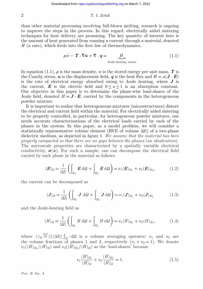
than other material processing involving full-blown melting, research is ongoingto improve the steps in the process. In this regard, electrically aided sinteringtechniques for heat delivery are promising. The key quantity of interest here isthe amount of heat generated from running a current through a material, denotedH (a rate), which feeds into the first law of thermodynamics,

rw − T : Vu + V · q = H .︸︷︷︸Joule-heating source

(1.1)

In equation (1.1), r is the mass density, w is the stored energy per unit mass, T isthe Cauchy stress, u is the displacement field, q is the heat flux and H = a(J · E)is the rate of electrical energy absorbed owing to Joule heating, where J isthe current, E is the electric field and 0 ≤ a ≤ 1 is an absorption constant.Our objective in this paper is to determine the phase-wise load-shares of theJoule field, denoted H = J · E, carried by the components in the heterogeneouspowder mixture.

It is important to realize that heterogeneous mixtures (microstructures) distortthe electrical and current field within the material. For electrically aided sinteringto be properly controlled, in particular, for heterogeneous powder mixtures, oneneeds accurate characterizations of the electrical loads carried by each of thephases in the system. In this paper, as a model problem, we will consider astatistically representative volume element (RVE of volume |U|) of a two-phasedielectric medium, as depicted in figure 1. We assume that the material has beenproperly compacted so that there are no gaps between the phases (an idealization).The microscale properties are characterized by a spatially variable electricalconductivity, s(x). For such a sample, one can decompose the electrical fieldcarried by each phase in the material as follows:

〈E〉U = 1|U|

(∫U1

E dU +∫

U2

E dU

)= v1〈E〉U1 + v2〈E〉U2 , (1.2)

the current can be decomposed as

〈J 〉U = 1|U|

(∫U1

J dU +∫

U2

J dU

)= v1〈J 〉U1 + v2〈J 〉U2 (1.3)

and the Joule-heating field as

〈H 〉U = 1|U|

(∫U1

H dU +∫

U2

H dU

)= v1〈H 〉U1 + v2〈H 〉U2 , (1.4)

where 〈·〉Udef= (1/|U|) ∫

U· dU is a volume averaging operator; v1 and v2 are

the volume fractions of phases 1 and 2, respectively (v1 + v2 = 1). We denotev1(〈H 〉U1/〈H 〉U) and v2(〈H 〉U2/〈H 〉U) as the ‘load-shares’ because

v1〈H 〉U1

〈H 〉U

+ v2〈H 〉U2

〈H 〉U

= 1. (1.5)

Proc. R. Soc. A

Electrically aided sintering 3

on March 7, 2012rspa.royalsocietypublishing.orgDownloaded from

appliedcurrent

Figure 1. A compacted powder with an applied current to help bond the component materials withJoule heating.

The objective of this paper is to determine the load-shares as functions of known(a priori) quantities,

v1〈H 〉U1

〈H 〉U

= F1(v1, s1, s2, 〈J 〉U, 〈E〉U) (1.6)

andv2

〈H 〉U2

〈H 〉U

= F2(v2, s1, s2, 〈J 〉U, 〈E〉U), (1.7)

where s1 and s2 are the conductivities of phase 1 and phase 2, respectively. Theoverall volume averages, 〈E〉U and 〈J 〉U, are considered known because they canbe determined by the boundary values from well-known results (discussed in §2):(i) the Average Electric Field Theorem and (ii) the Average Current Theorem.The presentation is as follows:

— expressions are developed for the current-field (J ) and electric-field (E)distribution for each component in the mixture;

— expressions are developed for the Joule-heating field current distributionfor each component in the materials (J · E);

— bounding principles are used to provide estimates of the overall responseof the material;

— asymptotic cases of extreme powder mixtures of insulators and super-conductors are considered;

— simple estimates for the time to heating are provided; and— extensions, involving numerical methods, are discussed.

Remark 1.1. The mathematical form for Joule heating can be motivated bytaking Faraday’s Law

V × E = −vBvt

(1.8)

Proc. R. Soc. A

4 T. I. Zohdi

on March 7, 2012rspa.royalsocietypublishing.orgDownloaded from

and Ampere’s Law

V × H = vDvt

+ J , (1.9)

where D is the electric field flux, H is the magnetic field, B is the magnetic fieldflux and forming the difference between the inner product of the electric field withAmpere’s Law and the inner product of the magnetic field with Faraday’s Law,

E · (V × H ) − H · (V × E)︸ ︷︷ ︸−V·(E×H )=−V·S

= E · J + E · vDvt

+ H · vBvt︸ ︷︷ ︸

= vWvt

, (1.10)

where W = 12(E · D + H · B) is the electromagnetic energy and S = E × H is

the Poynting vector. This relation can be rewritten as

vWvt

+ V · S = −J · E. (1.11)

Equation (1.11) is usually referred to as Poynting’s theorem. This can beinterpreted, for simple material laws, where the previous representation for Wholds, as stating that the rate of change of electromagnetic energy within avolume, plus the energy flowing out through a boundary, is equal to the negativeof the total work performed by the fields on the sources and conduction. Thiswork is then converted into thermo-mechanical energy (‘Joule heating’, H inequation (1.1)). Joule heating stems from ions being pulled through a mediumby electromagnetic fields, which generate heat when they collide with theirsurroundings.

Remark 1.2. In this work, we assume that the material has been properlycompacted, and we focus solely on the electrical heating aspects of this process.There has been considerable research activity in non-electrical compaction ofpowders, for example, see Brown & Abou-Chedid (1994), Fleck (1995), Tatzel(1996), Akisanya et al. (1997), Domas (1997), Anand & Gu (2000), Gu et al.(2001), Gethin et al. (2003), Zohdi (2003a) and Ransing et al. (2004).

Remark 1.3. Generally, for detailed pointwise information, for example,localized effects in the matrix ligaments between particles (‘hot spots’), oneneeds to solve boundary-value problems posed over a statistically RVE sampleof heterogeneous media. This will be discussed at the end of this paper.However, the essential issue is that time-transient effects lead to couplingof electrical and magnetic fields, and the only viable approach is to employdirect numerical techniques to solve for Maxwell’s equations. Generally, theseequations are strongly coupled. Additionally, if the local material propertiesare thermally sensitive, and Joule heating is significant, then the first lawof thermodynamics must also be solved, simultaneously. Numerical techniquesfor the solution of coupled boundary-value problems posed over heterogeneouselectromagnetic media, undergoing thermo-mechano-chemical effects can befound in Zohdi (2010).

Proc. R. Soc. A

Electrically aided sintering 5

on March 7, 2012rspa.royalsocietypublishing.orgDownloaded from

2. The controllable quantities: 〈J 〉U and 〈E〉U

For our model problem, two physically important test boundary (vU) loadingstates are notable on a sample of heterogeneous material (figure 1): (i) appliedelectric fields of the form E|vU = E and (ii) applied current field of the form J |vU =J , where E and J are constant electric field and current field vectors, respectively.Clearly, for these loading states to be satisfied within a macroscopic body undernon-uniform external loading, the sample must be large enough to possess smallboundary field fluctuations relative to its size. Therefore, applying (i)- or (ii)-typeboundary conditions to a large sample is a way of reproducing approximatelywhat may be occurring in a statistically representative microscopic sample ofmaterial within a macroscopic body. The following two results render 〈J 〉U and〈E〉U as controllable quantities, via the boundary loading.

— The Average Electric Field Theorem. Consider a sample with boundaryloading E|vU = E. We make use of the identity

V × (E ⊗ x) = (V × E) ⊗ x + E · Vx︸ ︷︷ ︸E

, (2.1)

and substitute this in the definition of the average electric field,

〈E〉U = 1|U|

∫U

(V × (E ⊗ x) − (V × E)︸ ︷︷ ︸=0

⊗x) dU = 1|U|

∫vU

n × (E ⊗ x) dA

= 1|U|

∫vU

n × (E ⊗ x) dA = 1|U|

(∫vU

(V × E) ⊗ x dU +∫

vU

E · Vx dU

).

(2.2)

Thus, if V × E = 0, then 〈E〉U = E, when E|vU = E.— The Average Current Field Theorem. Consider a sample with boundary

loading J |vU = J . We make use of the identity

V · (J ⊗ x) = (V · J )x + J · Vx︸ ︷︷ ︸J

, (2.3)

and substitute this in the definition of the average current,

〈J 〉U = 1|U|

∫U

(V · (J ⊗ x) − (V · J )︸ ︷︷ ︸=0

x) dU = 1|U|

∫vU

n · (J ⊗ x) dA

= 1|U|

∫vU

n · (J ⊗ x) dA = 1|U|

(∫vU

(V · J ) ⊗ x dU +∫

vU

J · Vx dU

).

(2.4)

Thus, if V · J = 0, then 〈J 〉U = J when J |vU = J .

Remark 2.1. The importance of the Average Electric Field Theorem and theAverage Current Field Theorem is that we can consider 〈E〉U and 〈J 〉U to becontrollable quantities, via E or J on the boundary. Applying these boundaryconditions should be made with the understanding that these idealizations

Proc. R. Soc. A

6 T. I. Zohdi

on March 7, 2012rspa.royalsocietypublishing.orgDownloaded from

reproduce what a RVE (which is much smaller than the structural componentof intended use) would experience within the system of intended use. Uniformloading is an idealization and would be present within a vanishingly smallmicrostructure relative to a finite-sized engineering (macro)structure. These typesof loadings are somewhat standard in computational analyses of samples ofheterogeneous materials (see Zohdi 2003b, 2010; Zohdi & Wriggers 2008; Ghosh2011; Ghosh & Dimiduk 2011).

Remark 2.2. In the analysis that follows, we will use the following energy–power relation:

〈H 〉U = 〈J · E〉U = 〈J 〉U · 〈E〉U, (2.5)

which is referred to as an ergodicity condition in statistical mechanics (Kröner1972; Torquato 2002) and as a Hill-type condition in the solid mechanics literature(Hill 1952). This is essentially a statement that the microenergy (power) mustequal the macroenergy (power). Equation (2.5) is developed by first splitting thecurrent and electric fields into mean (average) and purely fluctuating (zero mean)parts. For the current field, one has J = 〈J 〉U + J , where 〈J 〉U = 0 and for theelectric field E = 〈E〉U + E, where 〈E〉U = 0. The product yields

〈(〈J 〉U + J ) · (〈E〉U + E)〉U = 〈J 〉U · 〈E〉U + 〈J · E〉U (2.6)

because 〈J 〉U = 0 and 〈E〉U = 0. The ergodicity assumption is that 〈J · E〉U → 0,as the volume |U| → ∞ (relative to the inherent length scales in themicrostructure). The implication is that, as the sample becomes infinitely large,J · E is purely fluctuating and hence 〈J · E〉U = 0. In other words, the productof two purely fluctuating random fields is also purely fluctuating. These resultsare consistent with the use of the uniform boundary loadings introduced earlierbecause they can be shown to satisfy equation (2.5).

3. Concentration tensors and load-shares

A useful quantity that arises in the analysis of heterogeneous dielectric materialsis the effective conductivity, s∗, defined via2

〈J 〉U = s∗ · 〈E〉U, (3.1)

which is the ‘property’ (a relation between volume averages) used in micro–macroscale analyses. Decomposing the left-hand side yields

〈J 〉U = v1〈J 〉U1 + v2〈J 〉U2

= v1s1 · 〈E〉U1 + v2s2 · 〈E〉U2

= s1 · (〈E〉U − v2〈E〉U2) + v2s2 · 〈E〉U2

= (s1 + v2(s2 − s1) · CE ,2)︸ ︷︷ ︸s∗

·〈E〉U, (3.2)

2Implicitly, we assume that (i) the contact between the phases is perfect and (ii) the ergodicityhypothesis is satisfied (see Kröner (1972) or Torquato (2002)).

Proc. R. Soc. A

Electrically aided sintering 7

on March 7, 2012rspa.royalsocietypublishing.orgDownloaded from

where((1/v2)(s2 − s1)−1 · (s∗ − s1))︸ ︷︷ ︸

def=CE ,2

·〈E〉U = 〈E〉U2 . (3.3)

CE ,2 is known as the electric field concentration tensor. Thus, the product ofCE ,2 with 〈E〉U yields 〈E〉U2 . It is important to realize that once either CE ,2 ors∗ are known, the other can be computed.

In order to determine the concentration tensor for phase 1, we have fromequation (1.2)

〈E〉U1 = 〈E〉U − v2〈E〉U2

v1= (1 − v2CE ,2) · 〈E〉U

v1

def= CE ,1 · 〈E〉U, (3.4)

where

CE ,1 = 1v1

(1 − v2CE ,2) = 1 − v2CE ,2

1 − v2. (3.5)

Note that equation (3.5) implies

v1CE ,1︸ ︷︷ ︸phase-1 contribution

+ v2CE ,2︸ ︷︷ ︸phase-2 contribution

= 1. (3.6)

Similarly, for the current, we have

〈J 〉U = s∗ · 〈E〉U ⇒ s∗−1 · 〈J 〉U = C−1E ,2 · 〈E〉U2 = C−1

E ,2 · s−12 · 〈J 〉U2 . (3.7)

Thus,s2 · CE ,2 · s∗−1︸ ︷︷ ︸

CJ ,2

·〈J 〉U = 〈J 〉U2 (3.8)

andC J ,1 · 〈J 〉U = 〈J 〉U1 , (3.9)

where

C J ,1 = 1 − v2C J ,2

1 − v2= s1 · CE ,1 · s∗−1. (3.10)

We remark that equation (3.10) implies

v1C J ,1︸ ︷︷ ︸phase-1 contribution

+ v2C J ,2︸ ︷︷ ︸phase-2 contribution

= 1. (3.11)

Summarizing, we have the following results:

CE ,1 · 〈E〉U = 〈E〉U1, where CE ,1 = 1v1

(1 − v2CE ,2) = 1 − v2CE ,2

1 − v2,

CE ,2 · 〈E〉U = 〈E〉U2, where CE ,2 = 1v2

(s2 − s1)−1 · (s∗ − s1),

C J ,1 · 〈J 〉U = 〈J 〉U1, where C J ,1 = 1 − v2C J ,2

1 − v2= s1 · CE ,1 · s∗−1,

and C J ,2 · 〈J 〉U = 〈J 〉U2, where C J ,2 = s2 · CE ,2 · s∗−1.

Proc. R. Soc. A

8 T. I. Zohdi

on March 7, 2012rspa.royalsocietypublishing.orgDownloaded from

Remark 3.1. As a consequence of previous results, the Joule fields can bewritten in a variety of useful forms,

0 ≤ 〈H 〉Ui

def= 〈J 〉Ui · 〈E〉Ui = s−1i · 〈J 〉Ui · 〈J 〉Ui︸ ︷︷ ︸

in terms of phase averages of J

= si · 〈E〉Ui · 〈E〉Ui︸ ︷︷ ︸in terms of phase averages of E

= (C J ,i · 〈J 〉U) · (CEi · 〈E〉U)︸ ︷︷ ︸in terms of overall averages of J and E

= s−1i · (C J ,i · 〈J 〉U) · (C Ji · 〈J 〉U)︸ ︷︷ ︸

in terms of overall averages of J

= si · (CE ,i · 〈E〉U) · (CEi · 〈E〉U)︸ ︷︷ ︸in terms of overall averages of E

. (3.12)

4. Joule-heating load-shares

Using equation (3.12), the Joule fields can be bounded as follows (using theCauchy–Schwarz inequality):

〈H 〉Ui = (C J ,i · 〈J 〉U) · (CEi · 〈E〉U) ≤ ‖CE ,i‖‖C J ,i‖〈H 〉U

⇒ ‖CE ,i‖‖C J ,i‖ ≥ 〈H 〉Ui

〈H 〉U

. (4.1)

If the overall property is isotropic, and each of the constituents is isotropic (forexample, a microstructure comprised of an isotropic binder (fine-scale powder)embedded with randomly distributed isotropic particles), then we have thefollowing, CE ,i = CE ,i1 where, for a two-phase material,

CE ,1 = 11 − v2

s2 − s∗

s2 − s1and CE ,2 = 1

v2

s∗ − s1

s2 − s1, (4.2)

and C J ,i = CJ ,i1, leading to

CJ ,1 = s1

s∗(1 − v2)

(s2 − s∗

s2 − s1

)and CJ ,2 = s2

s∗v2

(s∗ − s1

s2 − s1

). (4.3)

Thus, in the case of isotropy, equation (4.1) asserts

CE ,1CJ ,1 ≥ 〈H 〉U1

〈H 〉U

and CE ,2CJ ,2 ≥ 〈H 〉U2

〈H 〉U

. (4.4)

The products of the concentration functions take the following forms:

CE ,1CJ ,1 = s1

s∗

(1

(1 − v2)

(s2 − s∗

s2 − s1

))2

(4.5)

and

CE ,2CJ ,2 = s2

s∗

(1v2

(s∗ − s1

s2 − s1

))2

. (4.6)

Proc. R. Soc. A

Electrically aided sintering 9

on March 7, 2012rspa.royalsocietypublishing.orgDownloaded from

Because the concentration functions depend on s∗, which in turn depends on s1,s2, v2 and the microstructure, we need to employ estimates for s∗. One class ofestimates are the Hashin–Shtrikman bounds (Hashin & Shtrikman 1962) for twoisotropic materials with an overall isotropic response,

s1 + v2

1/(s2 − s1) + (1 − v2)/3s1︸ ︷︷ ︸s∗,−

≤ s∗ ≤ s2 + 1 − v2

1/(s1 − s2) + v2/3s2︸ ︷︷ ︸s∗,+

, (4.7)

where the conductivity of phase 2 (with volume fraction v2) is larger than phase 1(s2 ≥ s1). Provided that the volume fractions and constituent conductivitiesare the only known information about the microstructure, the expressionsin equation (4.7) are the tightest bounds for the overall isotropic effectiveresponses for two-phase media, where the constituents are both isotropic. Acritical observation is that the lower bound is more accurate when the materialis composed of high-conductivity particles that are surrounded by a low-conductivity matrix (denoted case 1) and the upper bound is more accurate for ahigh-conductivity matrix surrounding low-conductivity particles (denoted case 2).

The previous comments on the accuracy of the lower or upper bounds canbe further qualitatively explained by considering the two cases with 50 per centlow-conductivity material and 50 per cent high-conductivity material. A materialwith a continuous low-conductivity (fine-scale powder) binder (50%) will isolatethe high-conductivity particles (50%), and the overall system will not conductelectricity well (this is case 1 and the lower bound is more accurate), while amaterial formed by a continuous high-conductivity (fine-scale powder) binder(50%) surrounding low-conductivity particles (50%, case 2) will, in an overallsense, conduct electricity better than case 1. Thus, case 2 is more closelyapproximated by the upper bound and case 1 is closer to the lower bound. Becausethe true effective property lies between the upper and lower bounds, one canconstruct the following approximation:

s∗ ≈ fs∗,+ + (1 − f)s∗,−, (4.8)

where 0 ≤ f ≤ 1. f is an unknown function of the microstructure. However, thegeneral trends are (i) for cases where the upper bound is more accurate, f > 1

2 ,and (ii) for cases when the lower bound is more accurate, f < 1

2 . Explicitly, for theproduct of concentration functions, embedding the effective property estimates,we have

CE ,1CJ ,1 ≈ s1

(fs∗,+ + (1 − f)s∗,−)

(1

(1 − v2)

(s2 − (fs∗,+ + (1 − f)s∗,−)

s2 − s1

))2

(4.9)

and

CE ,2CJ ,2 ≈ s2

(fs∗,+ + (1 − f)s∗,−)

(1v2

((fs∗,+ + (1 − f)s∗,−) − s1

s2 − s1

))2

. (4.10)

Remark 4.1. There are a vast literature of methods, dating back to Maxwell(1867, 1873) and Rayleigh (1892), to estimate the overall macroscopic propertiesof heterogeneous materials. For an authoritative review of (i) the general theory

Proc. R. Soc. A

10 T. I. Zohdi

on March 7, 2012rspa.royalsocietypublishing.orgDownloaded from

of random heterogeneous media, see Torquato (2002), (ii) for more mathematicalhomogenization aspects, see Jikov et al. (1994), (iii) for solid mechanics inclinedaccounts of the subject, see Hashin (1983), Mura (1993) and Nemat-Nasser &Hori (1999), (iv) for analyses of cracked media, see Sevostianov et al. (2001),and (v) for computational aspects, see Ghosh (2011), Ghosh & Dimiduk (2011)and Zohdi & Wriggers (2008). Tighter estimates, including generalized N-phasebounds can be found in Torquato (2002).3

Remark 4.2. The governing equation used in developing effective conductivitybounds is V · J = 0, which stems from taking the divergence of Ampere’s Law:V · (V × H − vD/vt − J ) = 0, one obtains, because V · (V × H ) = 0,

V ·(

vDvt

+ J)

= v

vtV · D︸ ︷︷ ︸

P

+V · J = vPvt

+ V · J = 0, (4.11)

where P is the charge per unit volume. Thus, if P = 0, then V · J = 0. Ifone employs the constitutive relation J = s · E, then this allows for Hashin–Shtrikman type estimates to be used for the effective conductivity, as does V · D =0 (which is valid only when P = 0) for estimates of the effective permittivity,〈D〉U = e∗ · 〈E〉U, when D = e · E. For example, one case when these two physicalsituations are compatible is when E = s−1 · J = e−1 · D ⇒ J = (s · e−1) · D.

5. Examples of Joule-heating load-sharing

(a) A general dielectric mixture

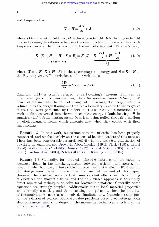
Figures 2 and 3 illustrate a surface (using f = 12) in parameter space (s1/s2, v2)

for the normalized Joule-heating load-share, vi(〈H 〉Ui/〈H 〉U), of each component,i = 1, 2. The plots illustrate the proportion of the Joule heating that will bedelivered to each phase in the system. Directly from equations (4.9) and (4.10),the load-share quantities of interest are

v1〈H 〉U1

〈H 〉U

≈ s1

v1(fs∗,+ + (1 − f)s∗,−)

(s2 − (fs∗,+ + (1 − f)s∗,−)

s2 − s1

)2

(5.1)

and

v2〈H 〉U2

〈H 〉U

≈ s2

v2(fs∗,+ + (1 − f)s∗,−)

((fs∗,+ + (1 − f)s∗,−) − s1

s2 − s1

)2

. (5.2)

The trends are

— for phase 1: decreasing the volume fraction of phase 2 (v2), for fixed s2/s1,leads to a larger load-share for phase 1, whereas decreasing the mismatchs2/s1, for a fixed v2, leads to an increased load-share for phase 1, for afixed volume fraction v2 and

3Such N-phase bounds go well beyond the simple Wiener bounds (Wiener 1910), (∑N

i=1 vis−1i )−1 ≤

s∗ ≤ ∑Ni=1 visi .

Proc. R. Soc. A

Electrically aided sintering 11

on March 7, 2012rspa.royalsocietypublishing.orgDownloaded from

0.20.4

0.60.8

24

68

10

–0.2

0

0.2

0.4

0.6

0.8

1.0

boun

d

1.0000.8750.7500.6250.5000.3750.2500.1250

22 1

Figure 2. A load-share surface in parameter space (s2/s1, v2) for the normalized Joule heating,v1(〈H 〉U1/〈H 〉U), for phase 1 (using f = 1/2). (Online version in colour.)

— for phase 2: increasing the volume fraction of phase 2 (v2), for fixed s2/s1,leads to a larger load-share for phase 2, whereas increasing the mismatchs2/s1, for a fixed v2, leads to an extremely slight change in the load-shareof phase 2 (it is virtually flat).

(b) An extreme mixture: high-conductivity (‘superconducting’) particles in alow-conductivity matrix

For the case of high-conductivity particles (phase 2) in a lower conductivitymatrix (phase 1), we have

1 s2

s1

def= a. (5.3)

Inserting this expression into the Hashin–Shtrikman bounds and taking the limitas a → ∞ yields (s2 tending to infinity)

s1

(1 + 2v2

1 − v2

)def= s1z ≤ s∗ ≤ ∞, (5.4)

Proc. R. Soc. A

12 T. I. Zohdi

on March 7, 2012rspa.royalsocietypublishing.orgDownloaded from

0.20.4

0.60.8

24

68

10

boun

d

0

0.2

0.4

0.6

0.8

1.01.0000.8750.7500.6250.5000.3750.2500.1250

22 1

Figure 3. A load-share surface in parameter space (s2/s1, v2) for the normalized Joule heating,v2(〈H 〉U2/〈H 〉U), for phase 2 (using f = 1/2). (Online version in colour.)

where the lower (Hashin–Shtrikman) bound is more accurate (f → 0).Correspondingly, for the concentration tensors for phase 1 (assuming isotropy),4

CE ,1 = 11 − v2

and CJ ,1 = 1z(1 − v2)

= 11 + 2v2

, (5.6)

and for phase 2 (particle),

CE ,2 = 0 and CJ ,2 = 1v2

(1 − 1

z

)= 3

1 + 2v2. (5.7)

Forming the products yields

CE ,1CJ ,1 =(

11 − v2

) (1

1 + 2v2

)(5.8)

andCE ,2CJ ,2 = 0. (5.9)

The expressions are appropriate for small v2 (superconducting particles in abinding matrix). Thus, we have for the load-share

11 + 2v2

≥ v1〈H 〉U1

〈H 〉U

, (5.10)

while for phase 2 (particle superconductor, no Joule field),

v2〈H 〉U2

〈H 〉U

= 0. (5.11)

4These expressions are asymptotically consistent with the identities

v1CE ,1 + v2CE ,2 = 1 and v1CJ ,1 + v2CJ ,2 = 1. (5.5)

Proc. R. Soc. A

Electrically aided sintering 13

on March 7, 2012rspa.royalsocietypublishing.orgDownloaded from

Remark 5.1. As v2 → 0 (no particle material; phase 2), the expressions collapseto restrictions on the pure matrix (here, phase 1) material.

(c) An extreme mixture: low-conductivity (‘insulator’) particles in ahigh-conductivity matrix

For the case of low-conductivity particles (phase 1) in a high-conductivitymatrix (phase 2), we have

1 � s1

s2

def= g. (5.12)

Inserting this expression into the Hashin–Shtrikman bounds and taking the limitas g → 0 (s1 tending to zero) yield

0 ≤ s∗ ≤ s2

(2v2

3 − v2

)def= s2l, (5.13)

where the upper (Hashin–Shtrikman) bound is more accurate (f → 1).Correspondingly, for the concentration tensors (as g → 0), for phase 1 (particle),

CE ,1 = 1 − l

1 − v2= 3

3 − v2and CJ ,1 = 0, (5.14)

and for phase 2 (matrix),

CE ,2 = l

v2= 2

3 − v2and CJ ,2 = 1

v2. (5.15)

The expressions are appropriate for large v2 (insulating particles in a bindingmatrix),

CE ,1CJ ,1 = 0 (5.16)

and

CE ,2CJ ,2 =(

23 − v2

) (1v2

). (5.17)

Thus, we have for the load-shares, for phase 1 (particle insulator, no Joule field),

v1〈H 〉U1

〈H 〉U

= 0, (5.18)

and for phase 2 (matrix),2

3 − v2≥ v2

〈H 〉U2

〈H 〉U

. (5.19)

Remark 5.2. As v2 → 1 (no particle (here, phase 1) material), the expressionscollapse to restrictions on the pure matrix (here, phase 2) material.

6. Conclusions and extensions

Short of large-scale numerical simulations, one can make rough estimates for thetime scales for heating the components materials to reach a target temperatureby ignoring stress–power and conduction in the first law (equation (1.1)). If we

Proc. R. Soc. A

14 T. I. Zohdi

on March 7, 2012rspa.royalsocietypublishing.orgDownloaded from

further assume that the temperature is uniform in each phase with ri w = rici˙〈q〉Ui

for each component material (i), we have

rici˙〈q〉Ui

= 〈H 〉Ui , (6.1)

which can be integrated to

〈q(t)〉Ui = 〈q(t = 0)〉Ui + 〈H 〉Ui

rciti ⇒ ti = rici〈Dq〉Ui

〈H 〉Ui

, (6.2)

where Dq = q(t) − q(t = 0). Specifically, for a two-phase material,

CE ,1CJ ,1〈H 〉U = s1

s∗

(1

(1 − v2)

(s2 − s∗

s2 − s1

))2

〈H 〉U ≥ 〈H 〉U1 (6.3)

and

CE ,2CJ ,2〈H 〉U = s2

s∗

(1v2

(s∗ − s1

s2 − s1

))2

〈H 〉U ≥ 〈H 〉U2 (6.4)

yield, with s∗ ≈ fs∗,+ + (1 − f)s∗,−, for phase 1, the time to heat the material tothe desired level (〈Dq〉U1),

t1 ≈ r1c1〈Dq〉U1

(s1/(fs∗,+ + (1 − f)s∗,−))((1/(1 − v2))((s2 − (fs∗,+ + (1 − f)s∗,−))/(s2 − s1)))2〈H 〉U

,

(6.5)and for phase 2 (〈Dq〉U2),

t2 ≈ r2c2〈Dq〉U2

(s2/(fs∗,+ + (1 − f)s∗,−))((1/v2)(((fs∗,+ + (1 − f)s∗,−) − s1)/(s2 − s1)))2〈H 〉U

.

(6.6)Clearly, once the design parameter estimates have been made to estimatethe processing time, more detailed information, for example, localized effectsin the matrix ligaments between particles (‘hot spots’), can be generatedvia only numerical simulation. To determine the generation of transientelectromagnetic fields, temperature fields, stress fields (owing to both Jouleheating and electromagnetically induced body forces) and chemical fields, thisrequires the solution to the time-transient forms of (i) Maxwell’s equations,(ii) the first law of thermodynamics, (iii) the balance of linear momentum, and(iv) reaction–diffusion laws. In order to accurately capture the coupled (transient)electromagnetic, thermal, mechanical and chemical behaviour of a complexmaterial, Zohdi (2010) addressed the modelling and simulation of such stronglycoupled systems using a staggered temporally adaptive finite difference timedomain (FDTD) method. Of particular interest was to provide a straightforwardmodular approach to finding the effective dielectric (electromagnetic) responseof a material, incorporating thermal effects, arising from Joule heating, whichalter the pointwise dielectric properties such as the electric permittivity,magnetic permeability and electric conductivity. Because multiple field couplingis present, a staggered, temporally adaptive scheme was developed to resolve theinternal microstructural electric, magnetic and thermal fields, accounting for thesimultaneous pointwise changes in the material properties. This approach alsoincorporated the coupled chemical and mechanical fields. We remark that there

Proc. R. Soc. A

Electrically aided sintering 15

on March 7, 2012rspa.royalsocietypublishing.orgDownloaded from

are a variety of computational electromagnetic methods. The most widely usedtechnique is the FDTD, which is ideally suited to the problems of interest in thiswork. However, there are other methods, such as (i) the Multi Resolution TimeDomain Method, which is based on wavelet-based discretization, (ii) the Finite-Element Method, which is based on discretization of variational formulations andwhich is ideal for irregular geometries,5 (iii) the Pseudo Spectral Time DomainMethod, which is based on Fourier and Chebyshev transforms, followed by alattice or grid discretization of the transformed domain, (iv) the Discrete DipoleApproximation, which is based on an array of dipoles solved iteratively with theconjugate gradient method and a fast Fourier transform to multiply matrices, and(v) the Method of Moments, which is based on integral formulations employingboundary-element method discretization, often accompanied by the fast multi-pole method to accelerate summations needed during the calculations, and (vi) thePartial Element Equivalent Circuit Method, which is based on integral equationsthat are interpreted as circuits in discretization cells.

In Zohdi (2010), FDTD was combined with a staggering solution frameworkto solve the coupled dielectric material systems of interest. The generalmethodology is as follows (at a given time increment): (i) each field equationis solved individually, ‘freezing’ the other (coupled) fields in the system, allowingonly the primary field to be active and (ii) after the solution of each field equation,the primary field variable is updated, and the next field equation is treated in asimilar manner. For an implicit type of staggering, the process can be repeated inan iterative manner, while for an explicit type, one moves to the next time stepafter one ‘pass’ through the system. As the physics changes, the field that is mostsensitive (exhibits the largest amount of relative non-dimensional change) dictatesthe time-step size. Because the internal system solvers within the staggeringscheme are also iterative and use the previously converged solution as theirstarting value to solve the system of equations, a field that is relatively insensitiveat given stage of the simulation will converge in very few internal iterations(perhaps even one). The overall goal was to deliver solutions where the staggering(incomplete coupling) error is controlled and the temporal discretization accuracydictates the upper limits on the time-step size. Generally speaking, the staggeringerror, which is a function of the time-step size, is time dependent and can becomestronger, weaker or possibly oscillatory, and is extremely difficult to ascertain apriori as a function of the time-step size. Therefore, to circumvent this problem,an adaptive staggering strategy was developed to provide accurate solutions byiteratively adjusting the time steps. Specifically, a sufficient condition for theconvergence of the presented fixed-point scheme was that the spectral radius(contraction constant of the coupled operator), which depends on the time-stepsize, must be less than unity. This observation was used to adaptively control thetime-step sizes while simultaneously controlling the coupled operator’s spectralradius, in order to deliver solutions below an error tolerance within a prespecifiednumber of desired iterations. This recursive staggering error control can allowfor substantial reduction of computational effort by the adaptive use of largetime steps, when possible. Furthermore, such a recursive process has a reducedsensitivity (relative to an explicit staggering approach) to the order in which

5In particular, see Demkowicz (2006) and Demkowicz et al. (2007) for the state-of-the-art inadaptive finite-element methods for Maxwell’s equations.

Proc. R. Soc. A

16 T. I. Zohdi

on March 7, 2012rspa.royalsocietypublishing.orgDownloaded from

the individual equations are solved because it is self-correcting. For more details,see Zohdi (2010). The further development of numerical methods for electricallyaided sintering simulation is under further investigation by the author.

The author expresses his gratitude to Ms Cora Schillig and Mr Gary Merrill of the Siemenscorporation for support of this research.

References

Akisanya, A. R., Cocks, A. C. F. & Fleck, N. A. 1997 The yield behavior of metal powders. Int.J. Mech. Sci. 39, 1315–1324. (doi:10.1016/S0020-7403(97)00018-0)

Anand, L. & Gu, C. 2000 Granular materials: constitutive equations and shear localization. J. Mech.Phys. Solids 48, 1701–1733. (doi:10.1016/S0022-5096(99)00066-6)

Brown, S. & Abou-Chedid, G. 1994 Yield behavior of metal powder assemblages. J. Mech. Phys.Solids 42, 383–398. (doi:10.1016/0022-5096(94)90024-8)

Demkowicz, L. 2006 Computing with hp-adaptive finite elements, vol. I. One- and two- dimensionalelliptic and maxwell problems. CRC Press. (doi:10.1201/9781420011685)

Demkowicz, L., Kurtz, J., Pardo, D., Paszynski, M., Rachowicz, W. & Zdunek, A. 2007 Computingwith hp-adaptive finite elements, vol. 2. Frontiers: three dimensional elliptic and Maxwellproblems with applications. CRC Press.

Domas, F. 1997 Eigenschaftprofile und Anwendungsübersicht von EPE und EPP. Technical reportof the BASF Company.

Fleck, N. A. 1995 On the cold compaction of powders. J. Mech. Phys. Solids 43, 1409–1431.(doi:10.1016/0022-5096(95)00039-L)

Gethin, D. T., Lewis, R. W. & Ransing, R. S. 2003 A discrete deformable element approachfor the compaction of powder systems. Model. Simul. Mater. Sci. Eng. 11, 101–114.(doi:10.1088/0965-0393/11/1/308)

Ghosh, S. 2011 Micromechanical analysis and multi-scale modeling using the Voronoi cell finiteelement method. CRC Press.

Ghosh, S. & Dimiduk, D. 2011 Computational methods for microstructure-property relations. NewYork, NY: Springer.

Gu, C., Kim, M. & Anand, L. 2001 Constitutive equations for metal powders: application topowder forming processes. Int. J. Plast. 17, 147–209. (doi:10.1016/S0749-6419(00)00029-2)

Hashin, Z. 1983 Analysis of composite materials: a survey. ASME J. Appl. Mech. 50, 481–505.(doi:10.1115/1.3167081)

Hashin, Z. & Shtrikman, S. 1962 A variational approach to the theory of effective magneticpermeability of multiphase materials. J. Appl. Phys. 33, 3125–3131. (doi:10.1063/1.1728579)

Hill, R. 1952 The elastic behaviour of a crystalline aggregate. Proc. Phys. Soc. A 65, 349.(doi:10.1088/0370-1298/65/5/307)

Jikov, V. V., Kozlov, S. M. & Olenik, O. A. 1994 Homogenization of differential operators andintegral functionals. New York, NY: Springer.

Kröner, E. 1972 Statistical continuum mechanics. CISM Lecture Notes, no. 92, Springer.Maxwell, J. C. 1867 On the dynamical theory of gases. Phil. Trans. Soc. Lond. 157, 49–88.

(doi:10.1098/rstl.1867.0004)Maxwell, J. C. 1873 A treatise on electricity and magnetism, 3rd edn. Oxford, UK: Clarendon

Press.Mura, T. 1993 Micromechanics of defects in solids, 2nd edn. Dordrecht, The Netherlands: Kluwer

Academic Publishers.Nemat-Nasser, S. & Hori, M. 1999 Micromechanics: overall properties of heterogeneous solids, 2nd

edn. Amsterdam, The Netherlands: Elsevier.Ransing, R. S., Lewis, R. W. & Gethin, D. T. 2004 Using a deformable discrete-element technique

to model the compaction behaviour of mixed ductile and brittle particulate systems. Phil. Trans.R. Soc. Lond. A 362, 1867–1884. (doi:10.1098/rsta.2004.1421)

Proc. R. Soc. A

Electrically aided sintering 17

on March 7, 2012rspa.royalsocietypublishing.orgDownloaded from

Rayleigh, J. W. 1892 On the influence of obstacles arranged in rectangular order upon propertiesof a medium. Phil. Mag. 32, 481–491.

Sevostianov, I., Gorbatikh, L. & Kachanov, M. 2001 Recovery of information ofporous/microcracked materials from the effective elastic/conductive properties. Mater.Sci. Eng. A 318, 1–14. (doi:10.1016/S0921-5093(01)01694-X)

Tatzel, H. 1996 Grundlagen der Verarbeitungstechnik von EPP-Bewährte und neue Verfahren.Technical report of the BASF Company.

Torquato, S. 2002 Random heterogeneous materials: microstructure & macroscopic properties. NewYork, NY: Springer.

Wiener, O. 1910 Zur Theorie der Refraktionskonstanten. Berichte über die Verhandlungen derKöniglich-Sächsischen Gesellschaft der Wissenshaften zu Leipzig. vol. Math. Phys Klasses, Band62, 256–277.

Zohdi, T. I. 2003a On the compaction of cohesive hyperelastic granules. Proc. R. Soc. Lond. A 459,1395–1401. (doi:10.1098/rspa.2003.1117)

Zohdi, T. I. 2003b Genetic design of solids possessing a random-particulate microstructure. Phil.Trans. R. Soc. A 361, 1021–1043. (doi:10.1098/rsta.2003.1179)

Zohdi, T. I. 2010 Simulation of coupled microscale multiphysical-fields in particulate-dopeddielectrics with staggered adaptive FDTD. Comput. Methods Appl. Mech. Eng. 199, 79–101.(doi:10.1016/j.cma.2010.06.032)

Zohdi, T. I. & Wriggers, P. 2008 Introduction to computational micromechanics, 2nd reprinting.Berlin, Germany: Springer.

Proc. R. Soc. A