estimation of laminated reservoir properties (a case …

POLITECNICO DI TORINO

Department of Environment, Land, and Infrastructure Engineering Master of Science in Petroleum Engineering

ESTIMATION OF LAMINATED RESERVOIR PROPERTIES (A CASE STUDY/ TORTONIAN

OIL RESERVOIR)

Supervisors: prof. Vera Rocca POLITECNICO DI TORINO Dr. Zakaria Hamdi HERIOT WATT UNIVERSITY

Candidate

Ibrahim Ahmed

July 2021

Ibrahim- Ahmed i _____________________________________________________________________________________

ABSTRACT

The lack of information for reservoir characterization has been a common problem

nowadays due to the current economic limitations on companies' capital expenses.

Therefore, the reservoir engineer has to fully exploit all available data and estimate the

unavailable reservoir characteristics. For lack of core data, the porosity is usually used

to estimate the permeability through classical correlations. However, predicting

permeability from porosity only and using classical relationships becomes unreliable

due to lithology and pore geometry effects. The objective of this study is to test the

integration between Flow Zone Indicator (FZI), Artificial Neural Network (ANN), and

Convergent Interpolation (CI) techniques to enhance the Tortonian reservoir description

in the Gamma oil field using the data of one exploratory well and four appraisal wells.

The reservoir description is done through 1) modeling the non-linear relationship

between the Tortonian reservoir properties, 2) calculating the effective porosity after

considering the effect of shale on well-log porosity measurements, 3) estimating the

permeability of appraisal wells (uncored wells), and 4) creating a permeability map for

the Tortonian oil reservoir.

The results showed that three rock types present within the Tortonian reservoirs. The

effective porosity and permeability logs were successfully estimated, and the

comparison between the created permeability log and quality check logs (GR and

porosity logs) reflected the high model quality. A permeability map has been created

and showed a direct relationship with the porosity map, which validates the

methodology. The reliability of the porosity/permeability relationship has increased up

to 90% after using the integrated techniques presented in the study.

The integration between FZI, ANN, and Convergent Interpolation techniques has

successfully modeled the non-linear intercourse between the porosity and permeability

of the Tortonian reservoir. The study enabled improving the complex reservoir

description economically with the minimum capital budget and available data.

Ibrahim- Ahmed ii _____________________________________________________________________________________

ACKNOWLEDGEMENTS

Full thanks to Allah for the gifts which Allah gives me. Firstly, from my heart, I would

be honored to declare my full thanks to my supervisors; Professor Vera Rocca, for her

help, motivation, and tracking of my work; definitely my full recognition to Dr. Zakaria

Hamdi for his gold tips, counseling, which leads to significant, clear, and polished

work.

I'm so eager to appreciate my parents, my sons (Adam and Younis), my wife for their

patience, face complex situations, especially in Covid-19 age. I'm eager to thank all my

colleagues, friends for their support.

Finally, thanks to the ENI scholarship official sponsors for their support and providing

all the necessary needs for the smooth and successful completion of the educational

process

Ibrahim- Ahmed iii _____________________________________________________________________________________

TABLE OF CONTENTS ABSTRACT ....................................................................................................................... i

ACKNOWLEDGEMENTS .............................................................................................. ii

LIST OF FIGURES ......................................................................................................... vi

LIST OF TABLES ......................................................................................................... viii

NOMENCLATURE ........................................................................................................ ix

1 INTRODUCTION .................................................................................................... 1

1.1 Introduction ........................................................................................................ 1

1.2 Statement of the Problem ................................................................................... 1

1.3 Objectives ........................................................................................................... 2

2 LITERATURE REVIEW ......................................................................................... 3

2.1 Reservoir properties. .......................................................................................... 3

2.1.1 Porosity ....................................................................................................... 3

2.1.1.1 Porosity classification .......................................................................... 3

2.1.2 Permeability ................................................................................................ 4

2.1.2.1 Permeability classification ................................................................... 5

2.2 Reservoir properties evaluation .......................................................................... 5

2.2.1 Coring & core analysis (CA): ..................................................................... 5

2.2.1.1 (RCA) .................................................................................................. 6

2.2.1.2 SCAL ................................................................................................... 6

2.2.2 Open hole-logs ............................................................................................ 7

2.2.2.1 Gamma-ray logs .................................................................................. 7

2.2.2.2 Porosity logs ........................................................................................ 8

2.2.2.3 Resistivity log .................................................................................... 10

2.3 Rock typing ...................................................................................................... 11

2.3.1 Flow zone indicator .................................................................................. 11

2.3.1.1 FZI validation .................................................................................... 14

2.4 Artificial neural networks (ANN) .................................................................... 15

2.4.1 ANN applications in the oil & gas industry .............................................. 17

3 METHODOLOGY ................................................................................................. 18

Ibrahim- Ahmed iv _____________________________________________________________________________________

3.1 Activity workflow ............................................................................................ 18

3.2 Input description ............................................................................................... 19

3.2.1 Core data ................................................................................................... 19

3.2.1.1 Messenian sand core .......................................................................... 19

3.2.1.2 Tortonian sand core ........................................................................... 20

3.2.2 Log data .................................................................................................... 20

3.2.2.1 Gamma-EX open hole logs ............................................................... 21

3.2.2.2 Gamma-1 open hole logs ................................................................... 23




3.2.2.6 Well logs correlation ......................................................................... 30

3.3 Estimation of FZI ............................................................................................. 31

3.3.1 Estimation of FZI flowchart ..................................................................... 31

3.4 Effective porosity estimation ........................................................................... 32

3.4.1 Effective porosity estimation flow chart for Tortonian reservoir ............. 32

3.5 Estimation permeability logs for uncored appraisal wells ............................... 33

3.5.1 Activity flow chart to assess the permeability for the appraisal wells ...... 33

3.5.2 ANN model for Gamma oil field .............................................................. 34

3.5.2.1 Data processing of Gamma-EX dataset ............................................. 34

3.5.2.2 Building the ANN model ................................................................... 34

3.5.2.3 Training the ANN on the training set of Gamma-EX ....................... 36

3.5.2.4 Predicting the FZI for the test set of Gamma-EX .............................. 37

3.5.2.5 Predicting the FZI for the appraisal wells ......................................... 37

3.6 Creating the permeability map of the Trotonian reservoir ............................... 38

4 RESULTS ............................................................................................................... 39

4.1 Tortonian's rock types ...................................................................................... 39

4.1.1 FZI statistical analysis .............................................................................. 39

4.2 FZI, effective porosity, and permeability logs for uncored wells .................... 40

Ibrahim- Ahmed v _____________________________________________________________________________________

4.2.1 Gamma-1 .................................................................................................. 40

4.2.2 Gamma-2 .................................................................................................. 41

4.2.3 Gamma-3 .................................................................................................. 42

4.2.4 Gamma-4 .................................................................................................. 43

4.3 Developed Tortonian's porosity and permeability relationship for the three rock

types 44

4.4 Permeability & effective porosity maps of the Tortonian reservoir ................ 45

4.4.1 Tortonian's permeability map ................................................................... 45

4.4.2 Tortonian's effective porosity map ........................................................... 46

5 CONCLUSION ....................................................................................................... 47

REFERENCES ............................................................................................................... 48

APPENDICES ................................................................................................................ 52

Appendix A tables of core data .................................................................................. 52

Appendix B tables of well-logs ................................................................................. 53

Appendix C tables of results ....................................................................................... 75

Ibrahim- Ahmed vi _____________________________________________________________________________________

LIST OF FIGURES

Figure 2-1 Engineering classification schematic .............................................................. 4

Figure 2-2 GR log vs. lithology ........................................................................................ 7

Figure 2-3 deep vs. shallow resistivity ........................................................................... 10

Figure 2-4 conventional K vs. PHI cross-plot ................................................................ 12

Figure 2-5 RQI – Φz Cross-plot ...................................................................................... 14

Figure 2-6 General ANN architecture ............................................................................ 15

Figure 2-7 Cost function VS. NO of epochs ................................................................... 16

Figure 3-1 Methodology flow chart ................................................................................ 18

Figure 3-2 Traditional cross-plot for Messenian sand .................................................... 19

Figure 3-3 Traditional cross-plot for Tortonian sand ..................................................... 20

Figure 3-4 Tortonian reservoir (cored interval) log data ................................................ 22

Figure 3-5 Statistical analysis of gamma-ray vs. depth .................................................. 22

Figure 3-6 Gamma-1 log data for Tortonian reservor .................................................... 23

Figure 3-7 Statistical distribution of gamma-ray vs. depth ............................................ 25

Figure 3-8 Gamma-2 log data for Tortonian formation .................................................. 26

Figure 3-9 Statistical distribution of gamma-ray values for upper Tortonian body sand

for well Gamma-3 ........................................................................................................... 27

Figure 3-10 Gamma-3 logs data for Tortonian formation .............................................. 28

Figure 3-11Gamma-4 logs data for Tortonian formation ............................................... 29

Figure 3-12 Well logs correlation ................................................................................... 30

Figure 3-13 Flowchart for FZI estimation ..................................................................... 31

Figure 3-14 Effective porosity estimation flow chart ..................................................... 32

Figure 3-15 Permeability estimation flow chart ............................................................. 33

Figure 3-16 ANN architecture for Gamma oil field ....................................................... 35

Figure 3-17 Python code to build ANN model ............................................................... 35

Figure 3-18 Training the ANN code ............................................................................... 36

Figure 3-19 Gamma-field ANN cost function plot ......................................................... 36

Figure 3-20 FZI Pred VS FZI Obs .................................................................................. 37

Figure 3-21 FZI prediction code ..................................................................................... 37

Figure 3-22 Permeability map creation workflow .......................................................... 38

Ibrahim- Ahmed vii _____________________________________________________________________________________

Figure 4-1 Tortonian's rock types ................................................................................... 39

Figure 4-2 FZI statistical analysis ................................................................................... 39

Figure 4-3 Created logs vs. quality check logs for Gamma-1 ....................................... 40

Figure 4-4 Created logs vs. quality check logs for Gamma-2 ........................................ 41



Figure 4-7 Porosity-permeability relationship of RT-1 .................................................. 44



Figure 4-10 Tortonian's permeability map ..................................................................... 45

Figure 4-11 Tortonian's effective porosity map .............................................................. 46

Ibrahim- Ahmed viii _____________________________________________________________________________________

LIST OF TABLES

Table 1 Messenian sand core data .................................................................................. 52

Table 2 Tortonian reservoir core data ............................................................................. 52

Table 3 Messenian sand (cored interval) log data. ......................................................... 53

Table 4 Tortonian sand (cored interval) log data. ........................................................... 53

Table 5 Gamma-1 logs data for interesting intervals of Tortonian FM .......................... 54


Table 7 Gamma-3 log data for interesting intervals of Tortonian FM ........................... 64


Table 9 FZI and its relevant log data of Gamma-EX ..................................................... 75

Table 10 FZI, effective porosity, and permeability logs of Gamma-1 ........................... 76




Ibrahim- Ahmed ix _____________________________________________________________________________________

NOMENCLATURE

𝑣𝑣 Apparent Flow Velocity, cm/s

𝑘𝑘 Permeability, Darcys,mD,m2

𝜇𝜇 Fluid Viscosity, cp

𝑑𝑑𝑑𝑑𝑑𝑑𝑑𝑑

Pressure Drop, atm/cm

𝛷𝛷 Total Porosity, fraction

𝑑𝑑𝑝𝑝 Pore Volume, cm3

𝐵𝐵𝑝𝑝 Bulk Volume, cm3

𝐼𝐼𝑠𝑠ℎ Shale Index, dimensionless

𝑣𝑣𝑠𝑠ℎ Volumetric Shale, dimensionless

𝛷𝛷𝐷𝐷 Density Derived Porosity, fraction 𝜌𝜌𝑙𝑙 Fluid Density, g/cm3

𝜌𝜌𝑏𝑏 Bulk Density, g/cm3

𝜌𝜌𝑚𝑚𝑚𝑚 Matrix Density, g/cm3

𝜌𝜌𝑏𝑏,𝑐𝑐 Corrected Bulk Density, g/cm3

𝜌𝜌𝑠𝑠ℎ Shale Density, g/cm3

𝛷𝛷𝐷𝐷𝑐𝑐 Corrected Density Porosity, fraction

𝛷𝛷𝑁𝑁𝑐𝑐 Corrected Neutron Porosity, fraction

𝛷𝛷𝑁𝑁𝑠𝑠ℎ Neutron Porosity / Shaly Intervals, fraction

𝛷𝛷𝑒𝑒 Effective Porosity, fraction

𝜏𝜏 Tortuosity

𝐹𝐹𝑠𝑠 Shape Factor

𝑆𝑆𝑔𝑔𝑔𝑔 Surface Area Per Grain Volume, 𝜇𝜇𝑚𝑚2

𝑅𝑅𝑅𝑅𝐼𝐼 Reservoir Quality Index, 𝜇𝜇𝑚𝑚

𝛷𝛷𝑧𝑧 Pore Volume Per Grain Volume

𝐹𝐹𝐹𝐹𝐼𝐼 Flow Zone Indicators, 𝜇𝜇𝑚𝑚

Ibrahim- Ahmed 1 _____________________________________________________________________________________

1 INTRODUCTION

1.1 Introduction

Nowadays, there is an inadequate information due to expensive operations to identify

reservoir characterization, especially for complex structure reservoirs. The reservoir

simulation software could not precisely simulate the reservoir structure and the grain

distribution within it. Therefore, the reservoir engineer should exploit the available data

to manage the reservoir in the optimal way to maximize hydrocarbons recovery.

The core analysis and lab correlations produce non-unique equations, which describe

the intercourses between the reservoir variables. Predicting one variable from the other

one using the direct relationship that comes from the lab analysis is unreliable due to the

complex geological structure of the reservoir. Hence, if the degree of the non-linearity is

reduced and correlates the independent variable with the reliant variable, it is feasible to

understand and manage such as a complex reservoir.

1.2 Statement of the Problem

Gamma field is an oil field consist of five wells. One of them is exploratory, and the others are appraisal wells to appraise the entire area of interest. Tortonian sand is the target reservoir penetrated by the five wells. Tortoninan sand shows a lamination phenomenon; hence the geological reservoir structure is complex.

The exploratory well is cored and logged; However, the appraisal wells are logged but uncored due to the economic limitations and the shortage of the available exploration budget.

The porosity/permeability relationship of Tortonian sand was derived from the routine core analysis test of the exploratory well. However, there is a high degree of non-linearity between the porosity and permeability because the variation in permeability depends not only on the porosity but also on the geological facies and the pore geometry; hence there is no unique mathematical equation that can describe the classical relationship between permeability and porosity. A full description of the Tortonion reservoir is required to maximize the oil recovery, which is a big challenge since:

1. The core data for the appraisal wells is not available 2. The classical porosity-permeability relationship drove from the core analysis

test of Gamma-EX is unreliable due to the complexity of the reservoir structure

Ibrahim- Ahmed 2 _____________________________________________________________________________________

1.3 Objectives

The objective of this study is to test the integration between Flow Zone Indicator

(FZI), Artificial Neural Network (ANN), and Convergent Interpolation (CI) techniques

for the sake of:

1. Modeling the non-linear relationship between the Tortonian reservoir

properties belong to the Gamma oil field

2. Calculating the effective porosity after considering the impact of shale

on well-log porosity measurements

3. Estimating the permeability of appraisal wells (uncored wells)

4. Creating a permeability map for the Tortonian oil reservoir

Ibrahim- Ahmed 3 _____________________________________________________________________________________

2 LITERATURE REVIEW

2.1 Reservoir properties.

The petroleum domain consists of three fundamental elements (Alyafei, 2019); these

elements are:

• Source rock • Cap-rock • Reservoir rock

The essential element in the petroleum system is the reservoir rock, which is the rock

that has sufficient storage capacity to store a significant amount of hydrocarbons and

can transmit the fluid (Amyx et al., 1960). The rock's ability to hold the fluid is the

porosity (void space), and permeability is a porous medium property that measures fluid

transmission capability for the formation (Ahmed, 2001).

The diagenetic process determines the structure of the inner reservoir and identifies

the porosity, permeability, and other physical characteristics of the reservoir rock

(Bjorlykkee et al., 2011; Clark, 1960). Carbonates and sandstones are generally

reservoir rocks that contain hydrocarbons. Tissot and Welte report that around 10% of

petroleum occurrences founded in fractured shale, igneous, and metamorphic rock

(Dandekar, 2015).

2.1.1 Porosity

From a mathematical standpoint, the porosity is fractional of the bulk volume of the

rock (Ahmed, 2001). Once the water plays an essential role in the transmission and

depositional processes, the water employs a part of the void space, isolating this part of

the void space. However, most pore space still has a movable fluid, water, oil, or gas

(Clark, 1960).

2.1.1.1 Porosity classification

(1) In terms of origin mode (Amyx et al., 1960) • Original • Induced

Ibrahim- Ahmed 4 _____________________________________________________________________________________

(2) Engineering classification (Alyafei, 2019) • Total porosity

• Effective porosity

• Ineffective porosity

The distinction among the subdivision of the porosity: total, effective, and ineffective

porosity highlighted through Figure 2-1.

Figure 2-1 Engineering classification schematic

(source: (Alyafei, 2019))

2.1.2 Permeability

The facility to move the fluid through rock spaces reflects the degree of rock

permeability (Clark, 1960). The rock permeability, which guides the fluid and controls

the flow rate, is an essential rock property. Henry Darcy mathematically defined this

rock characterization in 1856 (Ahmed, 2001). Indeed, in terms of mathematical

calculations, the equation that describes permeability is called - Darcy's Law (Amyx et

al., 1960) see equation (2-1)

𝑣𝑣 = −�𝑘𝑘𝜇𝜇�𝑑𝑑𝑑𝑑𝑑𝑑𝑑𝑑

(2-1)

Ibrahim- Ahmed 5 _____________________________________________________________________________________

Where 𝑣𝑣 = apparent flow velocity, cm/s

𝑘𝑘 = permeability, Darcys

𝜇𝜇 = fluid viscosity, cp

𝑑𝑑𝑑𝑑𝑑𝑑𝑙𝑙

= pressure drop, atm/cm

2.1.2.1 Permeability classification

The classification according to the number of phases saturates the rock's porous

(Alyafei, 2019). These classifications are:

• Effective permeability

• Absolute permeability

• Relative permeability (rock and fluid interaction)

2.2 Reservoir properties evaluation

2.2.1 Coring & core analysis (CA):

Core quality material is crucial for the success of an assessment of rock

characterization (Ubani & Adeboye, 2013). The coring program must minimize rock

damage and maximize rehabilitation. Core handling and preservation procedures used

before the core's arrival in the laboratory are equally important (Skopec, 1994).

There are two essential classes of testing for CA performed on core specimens

concerning the reservoir characteristics (Ahmed, 2001). These classes are:

(1) Routine CA tests

• Porosity (Φ) • Permeability (K) • Saturation (S)

(2) Special CA tests

• Relative Permeability • Wettability • Capillary pressure (CP) • Interfacial tension • Overburden pressure

Ibrahim- Ahmed 6 _____________________________________________________________________________________

2.2.1.1 (RCA)

RCA measures the essential rock characteristics under near-ambient conditions: Porosity and intrinsic permeability (Ubani & Adeboye, 2013).

Porosity evaluation:

Porosity is a function in bulk volume & pore volume described by equation (2-2)

(Dandekar, 2015) as follows:

Where 𝛷𝛷 = total porosity

𝑑𝑑𝑝𝑝= pore volume, cm3

𝐵𝐵𝑝𝑝= bulk volume, cm3

Vacuum saturation and Helium expansion are the main methods for measuring the

void spaces. However, the bulk volume is determined by calibrating the plug sample or

through the Archimedes principle (Dandekar, 2015; Ubani & Adeboye, 2013).

Permeability evaluation:

The intrinsic permeability of reservoir rock is measured directly by utilizing gas

flowing through the core plug under steady-state or transient conditions, such as air,

nitrogen, or helium. However, due to economic constraints, the liquid flowing through

the core plug is unpreferable (Dandekar, 2015; Ubani & Adeboye, 2013).

By injecting the air, nitrogen, or helium through the core plug under a controlled

flow rate, pressure, and well-known core plug geometry, it is easy to estimate the

permeability by using the proper form of Darcy's law (Ubani & Adeboye, 2013).

2.2.1.2 SCAL

The crucial task of SCAL is to identify the rock-fluid interaction properties, which

are embedded in the reservoir modeling to describe the fluid flow within the reservoir,

displacement processes, and transition zone thickness (Baker et al., 2015b).

𝛷𝛷 =𝑑𝑑𝑝𝑝𝐵𝐵𝑝𝑝

(2-2)

Ibrahim- Ahmed 7 _____________________________________________________________________________________

2.2.2 Open hole-logs

Lithology, porosity, permeability, formation water salinity, and rock stiffness are the

fundamental rock characteristics that affect logging measurements. The interpretation of

the logging tool response is essential to identify these properties (Asquith & Krygowski,

2014). The most crucial logging tool are:

• Gamma-ray (GR) logs

• Porosity logs

• Resistivity logs

2.2.2.1 Gamma-ray logs

Radionuclides, mainly potassium, uranium, and thorium decay, originate the present

application of the gamma-ray logs. Radio-active minerals mainly concentrate on the

shaly formation, which gives high gamma-ray values. However, the sandy formation or

free shale rock gives low gamma-ray readings (Asquith & Krygowski, 2014; Killeen,

1982). See Figure 2-2

Figure 2-2 GR log vs. lithology

( source: (Baker et al., 2015a))

Ibrahim- Ahmed 8 _____________________________________________________________________________________

Shale volume evaluation

The shaly formation contains clay minerals, organic matter as well. The structure,

laminar, and dispersed shale within reservoir rocks reduce the reservoir's storage

capacity, flow capacity, and effective porosity. Also, the shale affects the open-hole

logs measurements (Bassiouni, 1994; MK, 2017).

Gamma-ray index gives the first indication of the shale volume, which calculated by

the following equation (Asquith & Krygowski, 2014; Bassiouni, 1994):

Where 𝐼𝐼𝑠𝑠ℎ = shale index, dimensionless 𝐺𝐺𝑅𝑅𝑙𝑙𝑙𝑙𝑔𝑔 = the GR value from the log, API

𝐺𝐺𝑅𝑅𝑚𝑚𝑚𝑚𝑚𝑚 = the minimum GR reading from the log, API 𝐺𝐺𝑅𝑅𝑚𝑚𝑚𝑚𝑚𝑚 = the maximum GR value from the log, API The shale volume directly relates with the gamma-ray index through non-linear

empirical equations, which gives low shale volume compared to the linear

relationship(Asquith & Krygowski, 2014). Larionov (1969) represents the non-linear

relationship between the shale volume and the gamma-ray index for tertiary rock

equation (2-4) (Asquith & Krygowski, 2014; Bassiouni, 1994) as follows:

Where: 𝑣𝑣𝑠𝑠ℎ = shale volume, dimensionless

0.032 & 3.71 are the correlation constants for tertiary rocks

2.2.2.2 Porosity logs

Porosity logs measure the porosity indirectly based on nuclear measurements such as

density and neutron logs or acoustic measurements such as sonic logs (Asquith &

Krygowski, 2014).

Neutron logs (Φn, NPHI) measure the hydrogen amount retained into the porous

media in the absence of the shale. However, the density logs (Φd) measure the bulk

density (BHOB or RHO); the combination between neutron and density logs enhances

the estimation of rock lithology and detects hydrocarbon-bearing zone (Asquith &

Krygowski, 2014).

𝐼𝐼𝑠𝑠ℎ =𝐺𝐺𝑅𝑅𝑙𝑙𝑙𝑙𝑔𝑔 − 𝐺𝐺𝑅𝑅𝑚𝑚𝑚𝑚𝑚𝑚

𝐺𝐺𝑅𝑅𝑚𝑚𝑚𝑚𝑚𝑚 − 𝐺𝐺𝑅𝑅𝑚𝑚𝑚𝑚𝑚𝑚 (2-3)

𝑣𝑣𝑠𝑠ℎ = 0.083(23.7𝐼𝐼𝑠𝑠ℎ − 1) (2-4)

Ibrahim- Ahmed 9 _____________________________________________________________________________________

Effective porosity evaluation

The integration between fluid type, matrix nature, shale volume enhances reliable porosity estimation (Kamel & Mohamed, 2006). Therefore, the first step to evaluate rock porosity from the porosity logs is to correct the readings because the shale content affects the logging tool response (Bassiouni, 1994).

The equation (2-5) (Bassiouni, 1994; HLS, 2007) is used for calculating rock porosity from the density log:

Where 𝛷𝛷𝐷𝐷 = density derived porosity 𝜌𝜌𝑙𝑙 = fluid density, g/cm3

𝜌𝜌𝑏𝑏 = observed bulk density, g/cm3

𝜌𝜌𝑚𝑚𝑚𝑚 = bulk density of the rock matrix, for snd 2.64 g/cm3 (Asquith & Krygowski, 2014). The equation(2-6) (Miah, 2014) gives the corrected bulk density as:

Where 𝜌𝜌𝑏𝑏,𝑐𝑐 = corrected bulk density, g/cm3 𝜌𝜌𝑠𝑠ℎ = observed bulk density for shale interval, g/cm3

The formulation of calculating the corrected density derived porosity and adjusted

neutron porosity (HLS, 2007; Miah, 2014) as follows:

Where 𝛷𝛷𝑁𝑁𝑐𝑐 = corrected neutron porosity, fractional

𝛷𝛷𝑁𝑁 = neutron porosity observed from neutron log, fractional

𝛷𝛷𝑁𝑁𝑠𝑠ℎ = neutron porosity observed for shale interval, fractional

𝛷𝛷𝐷𝐷 =𝜌𝜌𝑚𝑚𝑚𝑚 − 𝜌𝜌𝑏𝑏𝜌𝜌𝑚𝑚𝑚𝑚 − 𝜌𝜌𝑙𝑙

(2-5)

𝜌𝜌𝑏𝑏,𝑐𝑐 = 𝜌𝜌𝑏𝑏 + 𝑣𝑣𝑠𝑠ℎ(𝜌𝜌𝑚𝑚𝑚𝑚 − 𝜌𝜌𝑠𝑠ℎ) (2-6)

𝛷𝛷𝐷𝐷𝑐𝑐 =𝜌𝜌𝑚𝑚𝑚𝑚 − 𝜌𝜌𝑏𝑏,𝑐𝑐

𝜌𝜌𝑚𝑚𝑚𝑚 − 𝜌𝜌𝑙𝑙 (2-7)

𝛷𝛷𝑁𝑁𝑐𝑐 = 𝛷𝛷𝑁𝑁 − 𝑣𝑣𝑠𝑠ℎ × 𝛷𝛷𝑁𝑁𝑠𝑠ℎ (2-8)

Ibrahim- Ahmed 10 _____________________________________________________________________________________

Finally, the following equation (HLS, 2007) determines the effective porosity:

2.2.2.3 Resistivity log

The rock skeleton is a high resistive material to transmit electric current. However, the bulk resistivity of the formation depends on the fluid that saturates the bore space. The hydrocarbons are non-conductive. The ability of the layer to conduct electric current depends on the water content and water salinity as well. The main tasks of the resistivity logs are (Asquith & Krygowski, 2014):

• Identify fluids contact • Indicate permeable layers

Figure 2-3 highlights how the resistivity logs indicate the permeable layers

Figure 2-3 deep vs. shallow resistivity ( source: (Asquith & Krygowski, 2014))

𝛷𝛷𝑒𝑒 = 𝛷𝛷𝑁𝑁𝑐𝑐 + 𝛷𝛷𝐷𝐷𝑐𝑐

2 (2-9)

Ibrahim- Ahmed 11 _____________________________________________________________________________________

2.3 Rock typing

The process by which reservoir rock is divided into geological units as a reservoir

building block is called rock typing; each block has the same geological facies, flow

capacity, and storage capacity. In the permeability-porosity framework, the integration

between the diagenesis properties and the depositional environment defines the rock

type. The supreme rock type has similar geological facies and the same reservoir

characteristic (Tavakoli, 2018).

There are four main rock typing techniques (Haikel et al., 2018), these are:

• Lucia

• Winland R35

• Flow zone indicator (FZI)

• Pore geometry structure (PGS)

2.3.1 Flow zone indicator

The most relevant approach of rock typing techniques is FZI, which depends on the

core data. The method divides the rock into hydraulic units(Amaefule et al., 1993).

Gunter (1997) defined the hydraulic unit as a volume of rock that has the same

characteristics and geological features; Tiab and Donaldson (2015) believed that the

reservoir unit is mappable, correlative, identifiable by wireline logs (Tavakoli, 2018).

Most hydrocarbon wells, due to economic constraints, are uncored. Non the less,

actual reservoir characteristics are often determined by core analysis tests. In the

absence of core data, permeability distribution is assessed from porosity logs based on

an empirical equation developed from the conventional cross-plot of porosity versus

logarithmic permeability (Amaefule et al., 1993; Soto B. et al., 2001).

Figure 2-4 shows a traditional cross plot of K versus Φ; only 14 % of the data fitted

by the power function trendline, which means the variation in permeability isn't

dependent only on porosity distribution. Lithology and pore geometry play an essential

role in describing the variation in permeability. However, the classical cross plot doesn't

consider the grain size distribution and lithological effect (Amaefule et al., 1993; Haikel

et al., 2018).

Ibrahim- Ahmed 12 _____________________________________________________________________________________

Figure 2-4 conventional K vs. PHI cross-plot

( source: (Haikel et al., 2018))

The generalized equation of the Kozeny-Carmen approach represents the pore throat

as capillary tubes to consider the effect of the geological feature on permeability

variation. The equation (2-10) (Amaefule et al., 1993) is described as follows:

where: 𝑲𝑲 = permeability, 𝝁𝝁𝒎𝒎𝟐𝟐

𝛷𝛷𝑒𝑒 = effective porosity

𝜏𝜏 = tortuosity

𝐹𝐹𝑠𝑠 = shape factor

𝑆𝑆𝑔𝑔𝑔𝑔 = surface area per unit grain volume, 𝜇𝜇𝑚𝑚2

The Kozeny-Carmen relationship describes the reservoir as a circular cylinder to

measure the flow capacity through the entire domain. However, in reality, the reservoir

is not a perfectly circular cylinder. Also, it is challenging to investigate and define the

pore geometry to calculate the tortuosity and surface area. So this assumption is not

applicable (Amaefule et al., 1993).

𝐾𝐾 =𝛷𝛷𝑒𝑒3

(1 −𝛷𝛷𝑒𝑒)2 �

1𝐹𝐹𝑠𝑠𝜏𝜏2𝑆𝑆𝑔𝑔𝑔𝑔2

� (2-10)

Ibrahim- Ahmed 13 _____________________________________________________________________________________

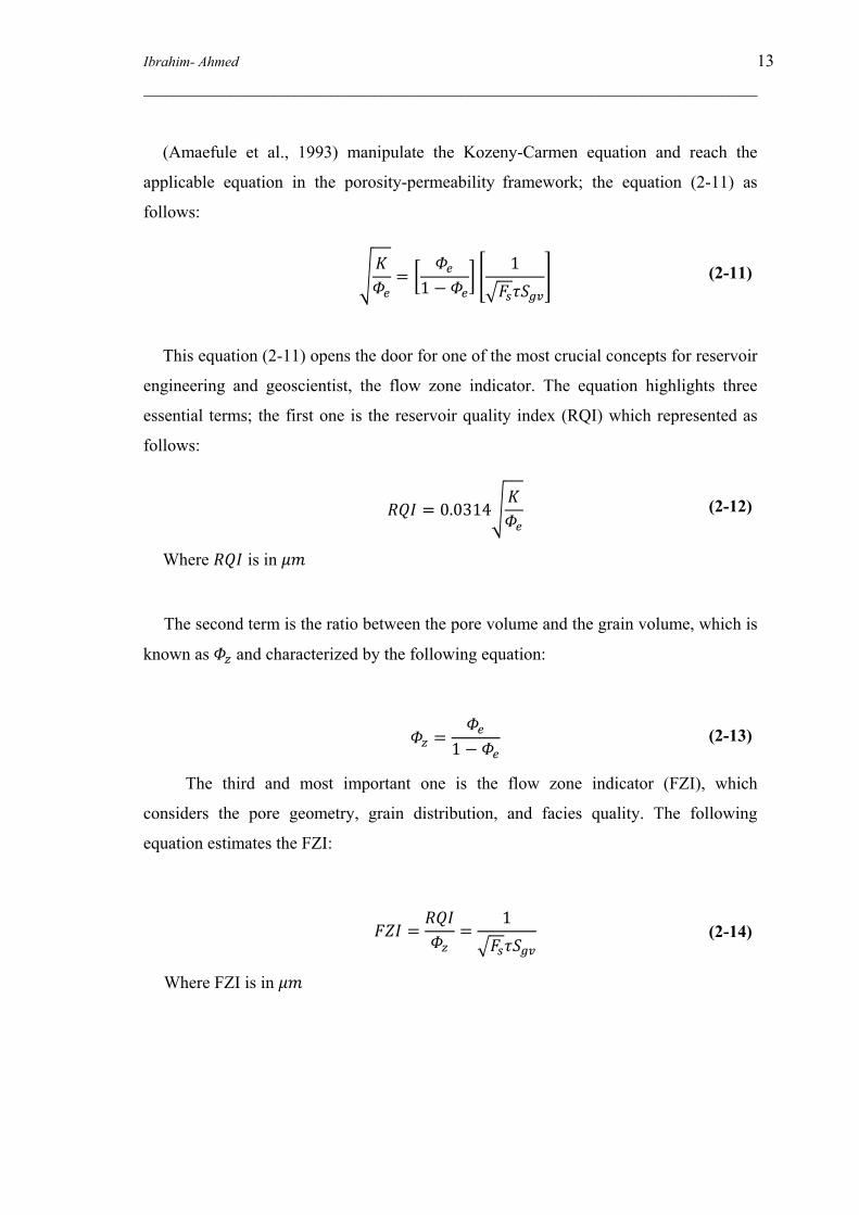
(Amaefule et al., 1993) manipulate the Kozeny-Carmen equation and reach the

applicable equation in the porosity-permeability framework; the equation (2-11) as

follows:

This equation (2-11) opens the door for one of the most crucial concepts for reservoir

engineering and geoscientist, the flow zone indicator. The equation highlights three

essential terms; the first one is the reservoir quality index (RQI) which represented as

follows:

Where 𝑅𝑅𝑅𝑅𝑅𝑅 is in 𝜇𝜇𝑚𝑚

The second term is the ratio between the pore volume and the grain volume, which is

known as 𝛷𝛷𝑧𝑧 and characterized by the following equation:

The third and most important one is the flow zone indicator (FZI), which

considers the pore geometry, grain distribution, and facies quality. The following

equation estimates the FZI:

Where FZI is in 𝜇𝜇𝑚𝑚

�𝐾𝐾𝛷𝛷𝑒𝑒

= �𝛷𝛷𝑒𝑒

1 − 𝛷𝛷𝑒𝑒� �

1�𝐹𝐹𝑠𝑠𝜏𝜏𝑆𝑆𝑔𝑔𝑔𝑔

� (2-11)

𝑅𝑅𝑅𝑅𝑅𝑅 = 0.0314�𝐾𝐾𝛷𝛷𝑒𝑒

(2-12)

𝛷𝛷𝑧𝑧 =𝛷𝛷𝑒𝑒

1 − 𝛷𝛷𝑒𝑒 (2-13)

𝐹𝐹𝐹𝐹𝑅𝑅 =𝑅𝑅𝑅𝑅𝑅𝑅𝛷𝛷𝑧𝑧

=1

�𝐹𝐹𝑠𝑠𝜏𝜏𝑆𝑆𝑔𝑔𝑔𝑔 (2-14)

Ibrahim- Ahmed 14 _____________________________________________________________________________________

By substituting the three terms into the equation (2-11) as logarithmic, the result will

be as follows:

𝑙𝑙𝑙𝑙𝑙𝑙𝑅𝑅𝑅𝑅𝑅𝑅 = 𝑙𝑙𝑙𝑙𝑙𝑙𝛷𝛷𝑧𝑧 + 𝑙𝑙𝑙𝑙𝑙𝑙𝐹𝐹𝐹𝐹𝑅𝑅 (2-15)

RQI - 𝛷𝛷𝑧𝑧 Cross-plot gives the number of the hydraulic units that have the same FZI

values and represented by straight line has unit slop ( see Figure 2-5).

Figure 2-5 RQI – Φz Cross-plot

(source: (Sritongthae, 2016))

Once FZI has been detected and by substituting into the equation (2-10), it is feasible

to appraise the permeability as follows:

Where 𝐾𝐾 is in millidarcy, FZI is in 𝜇𝜇𝑚𝑚.

2.3.1.1 FZI validation

(Abbas & Al Lawe, 2019; Biniwale, 2005; Dezfoolian, 2013; Hashim et al., 2017; Sritongthae, 2016; Uguru et al., 2005) tested the FZI method successfully for shale (Iraq), ( Australian fields),(Thailand fields), carbonate study, laminated sandstone, and Nigr delta. All of them predicted the reservoir characteristics effectively.

𝐾𝐾 = 1014(𝐹𝐹𝐹𝐹𝑅𝑅)2𝛷𝛷𝑒𝑒3

(1 − 𝛷𝛷𝑒𝑒)2 (2-16)

Ibrahim- Ahmed 15 _____________________________________________________________________________________

2.4 Artificial neural networks (ANN)

ANN mimics the human brain function, which is composed of millions of neurons.

Each group of neurons represents a layer where each layer has a specific job. Therefore,

integrating the layers is essential to complete the required mission (Basheer & Hajmeer,

2000).

ANN receives input signals through the input layer; each neuron of the input layer

retains one signal. Those signals transfer to other layers to be processed and produce

final outputs transferred from the output layer; the processing layers are called hidden

layers. The amount of neurons/units that make up the hidden sequence/ layer depends

on the signal processing complexity (Kay, 2001).

Each neuron of the input sequence relates to the hidden unit (neurons) by so-called

synapses, which allow the signal to transfer from the unit of the input sequence to the

unit of the hidden sequence. The weights represent the synapses that control the signal

transfer among the units; the weights behave as a filter for signals which permit free

noise signal to transfer (Nielsen, 2006; Rodolfo et al., 2002). See Figure 2-6.

Figure 2-6 General ANN architecture

( source : (Al-Aboodi et al., 2017))

Ibrahim- Ahmed 16 _____________________________________________________________________________________

ANN aims to model the non-linearity between the inputs and outputs variables

through learning the nature of variables dependency. So the starting point to build an

artificial neural network model is splitting the dataset into:

1. The training set helps the ANN to model the non-linearity between dependent

and independent variables.

2. The test set validates the ANN model.

One of the most important concepts is the misfit (cost function) between the

predicted output & the observed outputs. The cost function decreases by updating the

weights through adjusting the model parameters; these are:

1. The quantity of hidden stratification

2. The quantity of the hidden units

3. Trials number

4. Learning rate (ŋ), which is the percentage of updated weights

5. The ratio between the test data to the total data set

The backpropagation process renovates the weights according to their share in the

misfit; for each trial or optimization. Therefore, the cost function and the number of

trails cross-plot control the ANN model's parameters. For instance, Figure 2-7

highlights the learning rate (ŋ) effect on the misfit-number of epochs cross plot. The

misfit decreases dramatically with diminishing the learning rate (Nielsen, 2006).

Figure 2-7 Cost function VS. NO of epochs

https://www.powerthesaurus.org/stratification/synonyms

Ibrahim- Ahmed 17 _____________________________________________________________________________________

There are two backpropagation techniques to reach minimum misfit:

1. Batch-gradient descent (BGD)

2. Stochastic-gradient descent (SGD)

BGD, working on the complete matrix to research for the global error. It divides the

dataset into groups; each group has a local error. BGD aims to decrease the significant

misfit as a global error.

SGD reduces the local misfit for each element in the matrix domain, increasing the

computational cost. However, it gives high accuracy.

2.4.1 ANN applications in the oil & gas industry

In the absence of the essential data to describe the reservoir properties, the ANN

plays a vital role in estimating reservoir characteristics. The ANN method is tested

successfully by (Rodolfo et al., 2002; Soto B. et al., 2001; Uguru et al., 2005).

Ibrahim- Ahmed 18 _____________________________________________________________________________________

3 METHODOLOGY

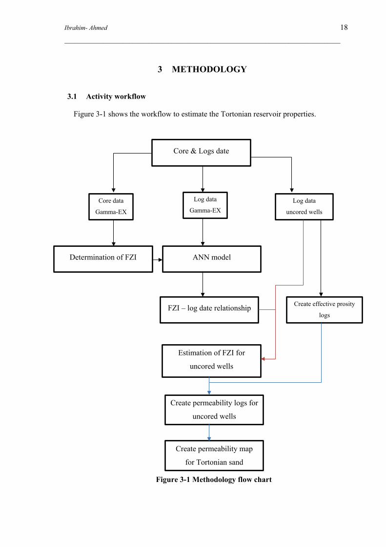
3.1 Activity workflow

Figure 3-1 shows the workflow to estimate the Tortonian reservoir properties.

Figure 3-1 Methodology flow chart

Estimation of FZI for

uncored wells

ANN model

Create effective prosity

logs

Create permeability logs for

uncored wells

Determination of FZI

FZI – log date relationship

Core data

Gamma-EX

Log data

Gamma-EX Log data

uncored wells

Core & Logs date

Create permeability map

for Tortonian sand

Ibrahim- Ahmed 19 _____________________________________________________________________________________

3.2 Input description

3.2.1 Core data

The coring operation performed during the exploratory well Gamma-EX drilling

activity shows two reservoir targets; these are

1. The upper target is Messenian sand

2. The lower target is Tortonian sand

The rock reservoir's unpreserved cores are acquired by the conventional coring bit.

Tortonian sand is the reservoir of interest because its reservoir structure is more

complex than the Messenian one.

3.2.1.1 Messenian sand core

The well Gamma-EX penetrates the Messenian reservoir and intersects the top of the

formation at 6702 FT-MD till the bottom of the sand at 6725 FT-MD; the entire interval

was cored and logged, the core has been cut, labeled, and packed in 1 feet boxes.

Thirteen plug samples were subjected to (RCA) test, where each sample

represents a specific depth. The RCA test gives Messenian reservoir porosity

and permeability (Table 1, appendix A).

The traditional K and Φ cross-plot graph shows that 33% of data fit the

relationship developed from the classical plot, and the owner company accepts

the ratio (as shown in Figure 3-2).

Figure 3-2 Traditional cross-plot for Messenian sand

y = 1.197e17.629x

R² = 0.3364

1

10

100

1000

0 0.05 0.1 0.15 0.2 0.25 0.3 0.35

Perm

eabi

lity

porosity

K VS PHI

Ibrahim- Ahmed 20 _____________________________________________________________________________________

3.2.1.2 Tortonian sand core

The well Gamma-EX penetrates the Tortonian reservoir and intersects the top of the

formation at 7187 FT-MD till the bottom of the sand at 7229 FT-MD; the entire interval

was cored and logged, the core has been cut, labeled, and packed in 1 feet boxes.

Twenty plug samples were subjected to (RCA) test, where each sample represents

a specific depth. The RCA test gives Messenian reservoir Φ and K (Table 2, appendix

A). The traditional K and Φ cross-plot graph shows that less than 1% of data fit the

relationship developed from the classical plot due to the lithology effect. (see Figure

3-3).

Figure 3-3 Traditional cross-plot for Tortonian sand

Tortoinian's porosity ranges from 0.05 to 0.2, and Tortoinian's permeability values

from 0.02 to 30 millidarcy. The core data is reliable because it is measured directly

through the lab. The company declares that the core data quality is high and efficient

due to handle and preservation procedures.

3.2.2 Log data

The indirect method helps to investigate the geology and petrophysical parameters of

the reservoir compared to the coring methodology as the direct method is well-logging.

The wireline logs that evaluate the Tortonian reservoir are:

1. Resistivity

2. Porosity

3. Gamma-ray

y = 0.4686e3.1663x

R² = 0.0039

0.01

0.1

1

10

100

0 0.05 0.1 0.15 0.2 0.25

perm

eabi

lity

porosity

K VS PHI

Ibrahim- Ahmed 21 _____________________________________________________________________________________

3.2.2.1 Gamma-EX open hole logs

Gamma-EX is the first well drilled in the Gamma oil field, which acted as the eye of

the engineers in the subsurface formations after the interpretation of the seismic data.

There was evidence of an amplitude anomaly that reflects the existence of hydrocarbons

accumulation. The logging tool response is affected by formation lithology,

petrophysical parameters, and clay minerals. Therefore, the change in the tool response

gives information about reservoir characteristics.

The triple-combo (wireline tool) was used to investigate the Tortonian and

Messenian reservoirs. The device is composed of three main parts:

1. Gamma source

2. Nuclear source

3. Electric source

Messenian reservoir

(Table 3, appendix B) shows the well-logs values for gamma-ray, neutron, and

density logs acquired using a triple-combo tool for the cored interval of Messenian

reservoir from 6702 FT-MD to 6725 FT-MD.

The gamma-ray recorded values in the range from 45.11 to 82.29 API; while the

neutron porosity obtained is in a range from 0.24 to 0.40 FT3/FT3, and the density log

readings among 2.1047 to 2.4491g/cm3, the values indicate different scale and units

between the three mentioned logs.

Tortonian reservoir

The well-logs values for gamma-ray, neutron, and density logs acquired using a

triple-combo tool for the cored interval of Tortonian reservoir from 7187 FT-MD to

7229 FT-MD (Table 4, appendix B).

The gamma-ray recorded values in the range from 45.54 to 83.09 API; while the

neutron porosity obtained is in a range from 0.1642 to 0.272 FT3/FT3, and the density

log readings among 2.368 to 2.5376 g/cm3, the values indicate different scale and units

between the three mentioned logs.

Ibrahim- Ahmed 22 _____________________________________________________________________________________

Figure 3-4 indicates the absence of the balloon effect between density-neutron logs

except at the depth 7206 FT-MD where the gamma-ray value tends to decrease,

indicating sandy facies.

Figure 3-4 Tortonian reservoir (cored interval) log data

The frequency of changes in the gamma-ray values is around 10 API per feet as an

average. It reaches 30 API per feet in some intervals, which gives an idea about the high

degree of non-linearity from routine core analysis results illustrated by the classical

porosity - permeability relationship.

Figure 3-5 shows the statistical distribution of gamma-ray values with formation

depth; the values change continuously with the depth, reflecting the complex

stratigraphic sequence and lamination effect.

Figure 3-5 Statistical analysis of gamma-ray vs. depth

0102030405060708090

7179

7180

7186

7187

7188

7194

7195

7196

7198

7202

7206

7207

7210

7211

7212

7216

7217

7218

7220

7221

ɣ ray

depth

ɣ-ray vs depth

Ibrahim- Ahmed 23 _____________________________________________________________________________________

3.2.2.2 Gamma-1 open hole logs

Gamma-1 is an appraisal well. It investigated the southwest area of the Gamma

field and the extension of the Tortonian reservoir in the lateral and vertical directions.

Core samples for Gamma-1 are not available due to economic issues and the high cost

of the coring operation. However, the logging data are available (Table 5, appendix B).

Figure 3-6 shows the log data for the entire reservoir from 7176 FT-MD until 7758

FT-MD. The well is vertical, so Tortonian thickness is 582 FT-SSTVD (177 M-

SSTVD) as isopach depth, which is considered a high thickness. However, the facies

are poor.

Figure 3-6 Gamma-1 log data for Tortonian reservor

Ibrahim- Ahmed 24 _____________________________________________________________________________________

Neutron-density logs; highlight the poor quality of sand facies, which affect the

resistivity readings. The resistivity log couldn't recognize the hydrocarbons bearing

zone and fluid contacts due to low permeability and high water salinity (180,000 ppm

NaCl). In addition, gamma-ray log response is affected by the lamination phenomena.

From the petrophysical evaluation, the net reservoir is 107 FT (33M), consisting of

six interesting intervals:

1. The first interval is from 7214 to 7228 FT-MD with an average gamma-ray

value of 69 API and resistivity value around 3.8 Ohm.M.

2. The second interval is from 7251 to 7273 FT-MD with an average Gamma-ray

value of 70 API and resistivity value of about 3Ohm.m.

3. The third interval is from 7511 to 7561 FT-MD with an average Gamma-ray

value of 69.6 API and resistivity value near 2.8 Ohm.M.

4. The fourth interval is from 7622 to 7627.83 FT-MD with an average Gamma-ray

value of 81 API and the value of resistivity approximately 4.4 Ohm.M, there are

two features regarding this interval, these are:

• gamma-ray reaches the maximum value

• resistivity response shows an increasing trend

5. The fifth interval is from 7635 to 7641 FT-MD with an average Gamma-ray

value of 89 API and resistivity value around 4.6 Ohm.M.

6. The last one is from 7687 to 7695 FT-MD, with an average Gamma-ray value of

60 API and resistivity value around 2.2 Ohm.M.

There is a direct relationship between GR readings and resistivity readings; this

relationship is unconventional. The effect of lithology and geological facies on logs tool

response highlighted by two observations:

1. Gamma-ray readings decrease for the sand formation, and in the presence of

HC, the resistivity values should increase, not decrease.

2. The difference between a low and high investigation resistivity response

disappears.

The net pay after the final evaluation is 21 feet, the net to gross is around 20% with

average porosity of 20%, and moderate water saturation is 50%.

Ibrahim- Ahmed 25 _____________________________________________________________________________________


Gamma-2 is an appraisal well. It investigated the southeast area of the Gamma field

and the extension of the Tortonian reservoir in the lateral and vertical directions. The

well is uncored, but the logging data are available (Table 6, appendix B).

Gamma-2 penetrates the Tortonian reservoir and intersects the top of the formation at

7154 FT-MD until the bottom at 7407 FT-MD. Hence, the thickness of the formation is

253 FT (77m), so it is relatively small compared to Gamma-1, but still, the extension of

the Tortonian reservoir exists in the southeast compartment of the Gamma field.

From the first look, the facies seemed to be improved. However, the complex

reservoir structure limits the reliability of resistivity logs to identify the existence of the

hydrocarbons and leads to mess interpretation. Concerning the balloon effect, some

intervals display the balloon effect, but only for limited intervals w.r.t the entire

thickness.

Once the lithology changes with the high frequency, the logging company adjusts the

logging tool's resolution to distinguish the lamination phenomena and the interference

between two laminae. The accuracy is adjusted for every 0.16 feet instead of 0.5 feet as

Gamma-1 to enhance the acquired data interpretation, mainly in the absence of the

coring operation and wireline formation tester.

The enhancement of the logging tool resolution enables a better petrophysical

evaluation; in the interval from 7201.8 to 7203.5 FT-MD, which is less than 1M, the

value of the gamma-ray decreases dramatically from 53.84 to 33.41 API as follows (see

Figure 3-7).

Figure 3-7 Statistical distribution of gamma-ray vs. depth

0

10

20

30

40

50

60

7201.8 7202.0 7202.2 7202.3 7202.5 7202.7 7202.8 7203.0 7203.2 7203.3 7203.5

ɣ ray

depth

ɣ-ray vs depth

Ibrahim- Ahmed 26 _____________________________________________________________________________________

The petrophysical evaluation; shows that the net reservoir in the southeast area is

around 100 FT, net-pay is approximately 15 FT, the net to gross is 15% with average

porosity of 20 %, SW is 40%, and the average gamma-ray value of 42 API.

Figure 3-8 shows the logs data of Gamma-2

Figure 3-8 Gamma-2 log data for Tortonian formation

Ibrahim- Ahmed 27 _____________________________________________________________________________________


Gamma-3 is an appraisal well. It investigated the northwest area of the Gamma field


well is uncored, but the logging data are available ( Table 7, appendix B).


7041 FT-MD until the bottom at 7210 FT-MD. Hence, the thickness of the formation is

169 FT (52m), so it is relatively small compared to Gamma-1 and Gamma-2, but still,

the extension of the Tortonian reservoir exists in the northwest compartment of the

Gamma field.

There are improvements in geological facies, petrophysical parameters contoured by

the porosity, and gamma-ray logs. This indicates the enhancement of the formation's

storage capacity; subsequently, oil volume increases, and resistivity readings increase.

The sand body from 7046 until 7074 FT-MD did not appear in the previous appraisal

wells, showing a different petrophysical parameter except for some interior intervals.

Therefore, it seems as clean body-sand without lamination effect, the appearance of the

clean-sand is due to the high structure of the well compared to the others. The statistical

distribution of the gamma-ray through that interval also shows consistency and

compatible values, most of the values between 27 to 34 API (see Figure 3-9).

Figure 3-9 Statistical distribution of gamma-ray values for upper Tortonian body

sand for well Gamma-3

Ibrahim- Ahmed 28 _____________________________________________________________________________________

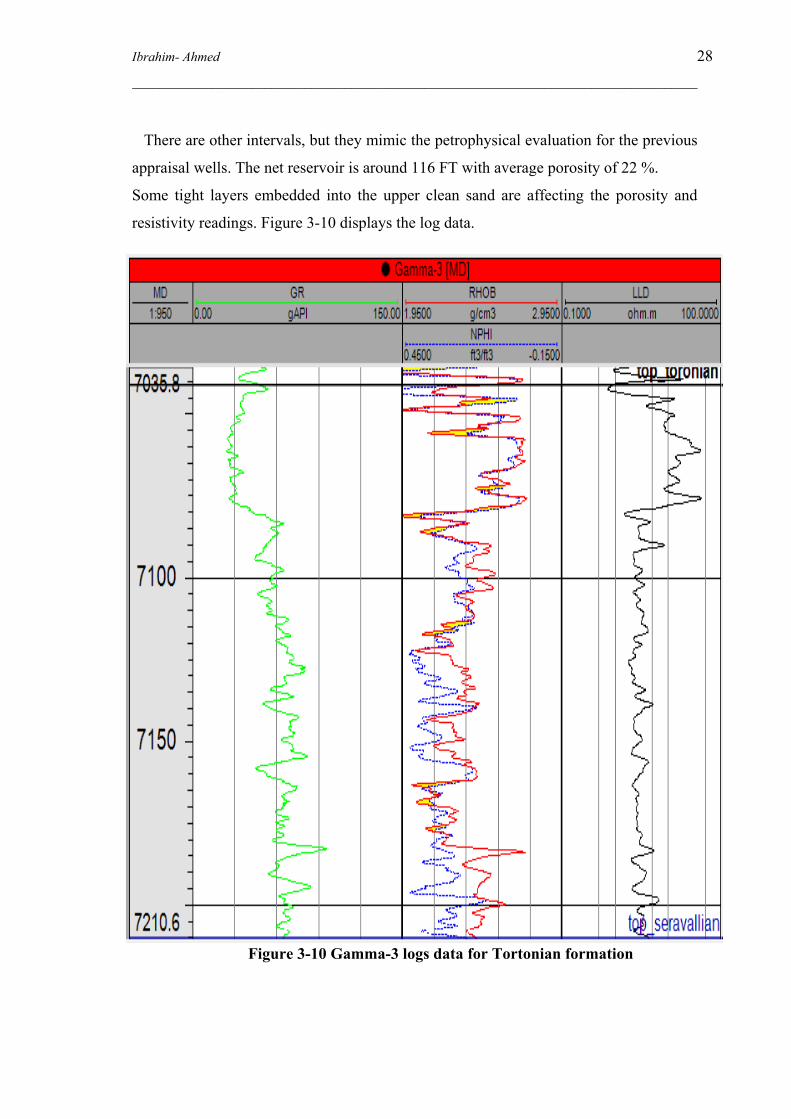
There are other intervals, but they mimic the petrophysical evaluation for the previous

appraisal wells. The net reservoir is around 116 FT with average porosity of 22 %.

Some tight layers embedded into the upper clean sand are affecting the porosity and

resistivity readings. Figure 3-10 displays the log data.

Figure 3-10 Gamma-3 logs data for Tortonian formation

Ibrahim- Ahmed 29 _____________________________________________________________________________________


Gamma-4 is an appraisal well. It investigated the northeast area of the Gamma field


well is uncored, but the logging data are available ( Table 8, appendix B).


7168 FT-MD until the bottom at 7323 FT-MD. Hence, the formation's thickness is 155

FT (47m), so it is relatively small compared to previous appraisal wells. However, the

extension of the Tortonian reservoir still exists in the northwest compartment of the

Gamma field.

The northeast region petrophysical parameters are identical to the south area except

the thickness, which is less than the south compartment, which contains Gamma-1 and

Gamma-2. Also, it matches with the central region of Gamma-EX, the average gamma-

values nearby 56 API and resistivity values approximately 2 Ohm.M. Figure 3-11

displays the log data.

Figure 3-11Gamma-4 logs data for Tortonian formation

Ibrahim- Ahmed 30 _____________________________________________________________________________________

3.2.2.6 Well logs correlation

Figure 3-12 gives information about the evolution of the Tortonian's thickness.

Figure 3-12 Well logs correlation

Ibrahim- Ahmed 31 _____________________________________________________________________________________

3.3 Estimation of FZI

3.3.1 Estimation of FZI flowchart

Figure 3-13 Flowchart for FZI estimation highlights the main steps to identify the flow units within the Tortonian reservoir.

Figure 3-13 Flowchart for FZI estimation

The main steps to estimate the FZI within the Tortonian reservoir are:

1. Calculate Φz from core porosity (Gamma-EX) for both:

• Tortonian reservoir

• Messenian reservoir

2. Calculate RQI from core permeability and porosity (Gamma-EX) for both:

• Tortonian reservoir

• Messenian reservoir

3. Plot RQI versus Φz on a log-log plot for Tortonian reservoir

4. Identify the flow unit within Tortonian reservoir

5. Register the results of Tortonian and Messenian reservoirs for future use.

Start with K &PHI (Φ) of core data

Compute

RQI by Eq.(2-12)

Φz by Eq.(2-13) FZI by Eq.(2-14)

Plot log RQI vs log Φz

---------------------------

FZI=RQI@Φz=1

Detect the numbers of the

hydraulic units and create

statistical histogram

Allocate for each plug sample an

FZI value

Prepare a table contains the

sample depth with the associated

FZI value as final result.

Ibrahim- Ahmed 32 _____________________________________________________________________________________

3.4 Effective porosity estimation

3.4.1 Effective porosity estimation flow chart for Tortonian reservoir

Figure 3-14 shows the main steps to calculate Tortonian's effective porosity

Figure 3-14 Effective porosity estimation flow chart

Gamma-ray and Φ logs are the most crucial tools to calculate Tortonian's effective

porosity, through:

1. Evaluating Tortonian's shale volume

2. Calibrating Tortonian's porosity readings by removing the shale effect

Log data

Calculate Ish

By Eq. (2-3)

Gamma-ray logs

Calculate Vsh

By Eq.(2-4)

NPHI- logs

BHOB- logs

Calculate Φe

By Eq.(2-9)

Calculate ΦNc

By Eq.(2-8)

Calculate ΦDc

By Eqs.(2-6)(2-7)

Ibrahim- Ahmed 33 _____________________________________________________________________________________

3.5 Estimation permeability logs for uncored appraisal wells

3.5.1 Activity flow chart to assess the permeability for the appraisal wells

Figure 3-15 shows the essential steps to evaluate the permeability in the absence of core data for the Gamma oil field.

Figure 3-15 Permeability estimation flow chart

Input data

FZI & log data of Gamma-EX

Validate the ANN model through

the test data

Create an ANN model by Python

Divide the data into training& test data

Set the model parameters

Train the model through the training set

Plot the cost function (misfit)

smooth

Decreasing trend to zero

Predict the FZI logs by the ANN

model for uncored wells

Effective

porosity logs

Predict the K using Eq.(2-16) for

uncored wells

yes No

Ibrahim- Ahmed 34 _____________________________________________________________________________________

3.5.2 ANN model for Gamma oil field

Python is used to create the ANN for the Gamma oil field to manage the relationship

between the dependent and independent variables for two reasons:

1. FZI is dependent on the core data and independent from well logs data.

2. The core data is not available for the appraisal wells.

The model is composed of the following sections:

1. Data processing of Gamma-EX dataset

2. Building the ANN model

3. Training the ANN on the training set of Gamma-EX

4. Predicting the FZI for the test set of Gamma-EX

5. Predicting the FZI for the appraisal wells

3.5.2.1 Data processing of Gamma-EX dataset

Deep learning needs a sufficient amount of data to train the model; the estimated FZI from the Messenian core data is used in addition to Tortonian FZI to train the model. The data set (Table 9, appendix C) is composed of:

1. FZI from the Gamma-EX core date 2. GR, NPHI, and RHOB well logs.

The data organized in a matrix, which consists of : • 33 rows (equal to the number of the core samples) • Four columns represent the dependent (log data) and independent (FZI)

variables. The normalization feature scaling is essential for the log data to have an equal effect

on the FZI values. After the normalization process for the input data, Python divides the

data into a test set and a training set. The ratio between the test set and the total data is

one of the model parameters. In Gamma field application, it is 30%.

3.5.2.2 Building the ANN model

The ANN for Gamma field consists of :

1. The input layer, which hosts the GR, NPHI, and RHOB

2. Two hidden layers, each one composed of 500 neurons (units)

3. The output layer, which produces the FZI value.

Ibrahim- Ahmed 35 _____________________________________________________________________________________

Figure 3-16 shows the ANN architecture for the Gamma oil field.

GR

NPHI FZI

RHOP

Input layer Hidden layer Output layer weights

Figure 3-16 ANN architecture for Gamma oil field

The rectifier activation function forced the model to respect the non-linear relation

for the entire domain. Figure 3-17 shows the python code to build the ANN model.

Figure 3-17 Python code to build ANN model

Ibrahim- Ahmed 36 _____________________________________________________________________________________

3.5.2.3 Training the ANN on the training set of Gamma-EX

Training the ANN is the most crucial section. The section functions are:

1. Identify the backpropagation technique

2. Identify the misfit (loss equation)

3. Train the ANN model

4. Identify the trails number

The ANN for the Gamma oil field uses the SGD (Adam optimizer) backpropagation

method, MSE, and the number of trails is 400 ( as shown in Figure 3-18).

Figure 3-18 Training the ANN code

the loss function shows a decreasing trend to zero (see Figure 3-19).

Figure 3-19 Gamma-field ANN cost function plot

Ibrahim- Ahmed 37 _____________________________________________________________________________________

3.5.2.4 Predicting the FZI for the test set of Gamma-EX

The tasks of this section are:

1. Predict the FZI for test data

2. Validate the ANN for further use

Figure 3-20 shows that around 90 of the test set predicted correctly from the model

Figure 3-20 FZI Pred VS FZI Obs

3.5.2.5 Predicting the FZI for the appraisal wells

This section aims to predict the FZI for uncored wells for further use, for instance, FZI

of Gamma-1 (see Figure 3-21).

Figure 3-21 FZI prediction code

Ibrahim- Ahmed 38 _____________________________________________________________________________________

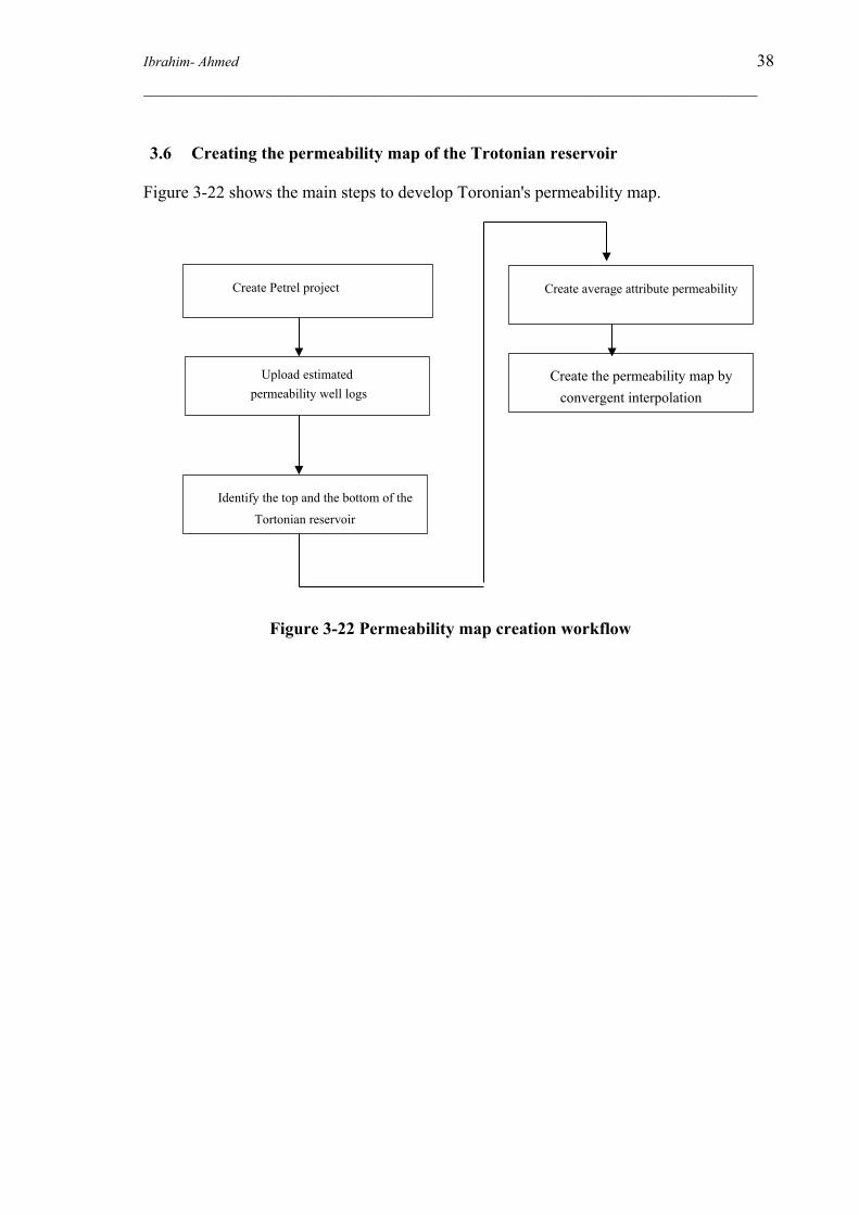
3.6 Creating the permeability map of the Trotonian reservoir

Figure 3-22 shows the main steps to develop Toronian's permeability map.

Figure 3-22 Permeability map creation workflow

Create Petrel project

Upload estimated permeability well logs

Create the permeability map by convergent interpolation

Create average attribute permeability

Identify the top and the bottom of the

Tortonian reservoir

Ibrahim- Ahmed 39 _____________________________________________________________________________________

4 RESULTS

4.1 Tortonian's rock types

Tortonian's rock types are three based on the FZI technique (as shown in Figure 4-1)

Figure 4-1 Tortonian's rock types

4.1.1 FZI statistical analysis

Flow zone indicators show range from 0.06 to 2.31𝜇𝜇𝜇𝜇 (as shown in Figure 4-2)

Figure 4-2 FZI statistical analysis

0.001

0.01

0.1

1

10

0.01 0.1 1

RQI

ᵠz

RT-FZI

RT-FZIFZI 3FZI 2FZI 1

0

0.5

1

1.5

2

2.5

1 2 3 4 5 6 7 8 9 10 11 12 13 14 15 16 17 18 19 20

FZI v

alue

plug sample's number

FZI statistical analysis

Ibrahim- Ahmed 40 _____________________________________________________________________________________

4.2 FZI, effective porosity, and permeability logs for uncored wells

4.2.1 Gamma-1

Figure 4-3 shows two sets of logs of the well (Gamma-1). These are: 1. Created logs ( FZI, K, and Φe)

2. Quality check logs ( GR, NPHI, and RHOB)

Figure 4-3 Created logs vs. quality check logs for Gamma-1

The comparison between created and quality check logs reflects the high model quality.

(Table 10, appendix C) shows the created log readings for curious intervals.

Ibrahim- Ahmed 41 _____________________________________________________________________________________

4.2.2 Gamma-2






Ibrahim- Ahmed 42 _____________________________________________________________________________________

4.2.3 Gamma-3






Ibrahim- Ahmed 43 _____________________________________________________________________________________

4.2.4 Gamma-4






Ibrahim- Ahmed 44 _____________________________________________________________________________________

4.3 Developed Tortonian's porosity and permeability relationship for the three rock types

1. For RT-1, the porosity and permeability relationship has a determination

coefficient value of 0.95. The porosity ranges from 15 to 37 %, and the

permeability ranges from 15 to 374 millidarcy (as shown in Figure 4-7).

Figure 4-7 Porosity-permeability relationship of RT-1



permeability ranges from 1 to 33 millidarcy (as shown in Figure 4-8).


y = 2.2864e13.531x

R² = 0.9791

1

10

100

1000

0 0.05 0.1 0.15 0.2 0.25 0.3 0.35 0.4

perm

eabi

lity

porosity

RT-1

y = 0.2074e18.792x

R² = 0.9781

0.1

1

10

100

0 0.05 0.1 0.15 0.2 0.25 0.3 0.35

perm

eabi

lity

porosity

RT-2

Ibrahim- Ahmed 45 _____________________________________________________________________________________



permeability ranges from 0.025 to 4.5 millidarcy (as shown in Figure-

4-9).


4.4 Permeability & effective porosity maps of the Tortonian reservoir

4.4.1 Tortonian's permeability map Figure 4-10 shows Tortonian's permeability map created by Petrel software.

Figure 4-10 Tortonian's permeability map

y = 0.0204e28.326x

R² = 0.9443

0.01

0.1

1

10

0 0.05 0.1 0.15 0.2 0.25

perm

eabi

lity

porosity

RT-3

Ibrahim- Ahmed 46 _____________________________________________________________________________________

4.4.2 Tortonian's effective porosity map

Figure 4-11 shows Torontonian's effective porosity map created by Petrel software

and used to check the quality of the permeability map.

Figure 4-11 Tortonian's effective porosity map

Ibrahim- Ahmed 47 _____________________________________________________________________________________

5 CONCLUSION

The integration between flow zone indicator, artificial neural networks, and convergent

interpolation techniques has been successfully tested through developing the

permeability map of the complex Tortonian reservoir structure. Based on the results of

this study, the following conclusions have been drawn:

1. The techniques used in this study successfully modeled the porosity and

permeability relationship and increased the model reliability up to 90% (the

developed relationships have fitted more than 90% of the data).

2. The FZI technique showed the presence of three different rock types

within the Tortonian reservoir.

3. The reliability of the porosity log readings has increased after removing

the effect of shale and improved the effective porosity estimation from the well-

logs.

4. The integration between FZI, ANN, and calibrating the porosity logs

readings has successfully allowed the estimation of reservoir permeability for un-

cored wells.

5. The permeability map shows that the well Gamma-3 penetrates the

northwest area that has the highest reservoir quality.

6. The reservoir quality increases from south to north, which is inversely

proportional to the reservoir thickness.

7. The reservoir thickness decreases in the upper reservoir structure.

Therefore, the overburden pressure declines, and the pore space compaction

diminishes, and the effective porosity increases.

8. Finally, the developed relationship showed that there is a direct

relationship between the effective porosity and permeability, which validates the

petro-physical evaluation presented in the study.

Ibrahim- Ahmed 48 _____________________________________________________________________________________

REFERENCES

Abbas, M. A., & Al Lawe, E. M. (2019). Clustering analysis and flow zone indicator for

electrofacies characterization in the upper shale member in Luhais oil field,

southern Iraq. Society of Petroleum Engineers - Abu Dhabi International

Petroleum Exhibition and Conference 2019, ADIP 2019.

https://doi.org/10.2118/197906-ms

Ahmed, T. (2001). Reservoir Engineering handbook. In Reservoir Engineering

Handbook.

Al-Aboodi, A. H., Al-Abadi, A. M., & T. Ibrahim, H. (2017). A Committee Machine

with Intelligent Systems for Estimating Monthly Mean Reference

Evapotranspiration in an Arid Region. Research Journal of Applied Sciences,

Engineering, and Technology, 14(10), 386–398.

https://doi.org/10.19026/rjaset.14.5131

Alyafei, N. (2019). Fundamentals of reservoir rock properties. In Fundamentals of

Reservoir Rock Properties (Issue January). https://doi.org/10.1007/978-3-030-

28140-3

Amaefule, J. O., Altunbay, M., Tiab, D., Kersey, D. G., & Keelan, D. K. (1993).

Enhanced reservoir description: using core and log data to identify hydraulic (flow)

units and predict permeability in uncored intervals/ wells. Proceedings - SPE

Annual Technical Conference and Exhibition, Omega(c), 205–220.

https://doi.org/10.2523/26436-ms

Amyx, J. W., Jr, D. ; B., & Whiting, R. L. (1960). Petroleum Reservoir

Engineering.pdf.

Asquith, G., & Krygowski, D. (2014). Basic Well Log Analysis Second Edition for

Geologists. In Dictionary Geotechnical Engineering/Wörterbuch GeoTechnik.

Baker, R. O., Yarranton, H. W., & Jensen, J. L. (2015a). Openhole Well Logs—Log

Interpretation Basics. In Practical Reservoir Engineering and Characterization.

https://doi.org/10.1016/b978-0-12-801811-8.00009-2

Baker, R. O., Yarranton, H. W., & Jensen, J. L. (2015b). Special Core Analysis—Rock–

Fluid Interactions. In Practical Reservoir Engineering and Characterization.

https://doi.org/10.1016/b978-0-12-801811-8.00008-0

Ibrahim- Ahmed 49 _____________________________________________________________________________________

Basheer, I. A., & Hajmeer, M. (2000). Artificial neural networks: fundamentals,

computing, design, and application. Journal of Microbiological Methods, 43(1), 3–

31. https://doi.org/10.1016/S0167-7012(00)00201-3

Bassiouni, Z. (1994). Theory, measurements, and interpretation of well-logs. In Journal

of Petroleum Science and Engineering (Vol. 13, Issues 3–4).

https://doi.org/10.1016/0920-4105(95)90010-1

Biniwale, S. (2005). An integrated method for modeling fluid saturation profiles and

characterizing geological environments using a modified FZI approach: Australian

fields case study. Proceedings - SPE Annual Technical Conference and Exhibition,

Student 4, 4847–4864. https://doi.org/10.2118/99285-stu

Bjorlykkee, K., Faleide, J. I., Roy H. Gabrielsen, Nils-Martin Hanken, Kaare Høeg, J.

J., Martin Landrø, Nazmul Haque Mondol, J. N., & Nielsen, and J. K. (2011).

Petroleum Geoscience: From Sedimentary Environments to Rock Physics.

Clark, N. (1960). Elements of petroleum reservoir.pdf.

Dandekar, A. (2015). Petroleum reservoir rock and fluid properties. In Methods of Soil

Analysis, Part 1: Physical and Mineralogical Properties, Including Statistics of

Measurement and Sampling. https://doi.org/10.2134/agronmonogr9.1.c21

Dezfoolian, M. A. (2013). Flow zone indicator estimation based on petrophysical

studies using an artificial neural network in a southern Iran reservoir. Petroleum

Science and Technology, 31(12), 1294–1305.

https://doi.org/10.1080/10916466.2010.542421

Haikel, S., Rosid, M. S., & Haidar, M. W. (2018). Study comparative rock typing

methods to classify rock type carbonate reservoir Field “s” East Java. Journal of

Physics: Conference Series, 1120(1), 0–10. https://doi.org/10.1088/1742-

6596/1120/1/012047

Hashim, N. S., Zakaria, A. F., & Ishak, N. A. (2017). An innovative approach towards

improving the relationship between flow zone indicators with lithofacies: A case

study in carbonate oil field, middle east. Society of Petroleum Engineers - SPE

Reservoir Characterisation and Simulation Conference and Exhibition, RCSC

2017, 799–825. https://doi.org/10.2118/186005-ms

HLS, A. (2007). Basic logic interpretation. In Classical and Nonclassical Logics (Issue

May). https://doi.org/10.2307/j.ctv15r582q.16

Ibrahim- Ahmed 50 _____________________________________________________________________________________

Kamel, M. H., & Mohamed, M. M. (2006). Effective porosity determination in

clean/shaly formations from acoustic logs with applications. Journal of Petroleum

Science and Engineering, 51(3–4), 267–274.

https://doi.org/10.1016/j.petrol.2006.01.007

Kay, A. (2001). Artificial Neural Networks | Computerworld. Computer World.

https://www.computerworld.com/article/2591759/artificial-neural-networks.html

Killeen, P. G. (1982). Gamma-ray logging and interpretation. Developments in

Geophysical Exploration Methods - 3, 95–150. https://doi.org/10.1007/978-94-

009-7349-7_4

Miah, M. I. (2014). Porosity assessment of gas reservoir using wireline log data: A case

study of Bokabil formation, Bangladesh. Procedia Engineering, 90, 663–668.

https://doi.org/10.1016/j.proeng.2014.11.789

MK, G. A. (2017). Determination of Shale Types using Well Logs. International

Journal Of Petrochemical Science & Engineering, 2(5), 274–280.

https://doi.org/10.15406/ipcse.2017.02.00051

Nielsen, M. (2006). Neural Networks and Deep Learning. In The Machine Age of

Customer Insight. https://doi.org/10.1108/978-1-83909-694-520211010

Rodolfo, S. B., Torres, F., Arango, S., Cobaleda, G., Holditch, S., & Wu, C. (2002).

How to Improve Reservoir Characterization Models Using Intelligent Systems. 2,

387–417. https://doi.org/10.1007/978-3-7908-1807-9_16

Skopec, R. A. (1994). proper coring and well-site core handling procedures: the first

step toward reliable core analysis. Journal of Petroleum Technology, 2815.

Soto B., R., Torres, F., Arango, S., & Cobaleda, G. (2001). Improved Reservoir

Permeability Models From Flow Units And Soft Computing Techniques: A Case

Study, Suria And Reforma-Libertad Fields, Colombia. 1–10.


Sritongthae, W. (2016). Petrophysical Rock Typing : Enhanced Permeability Prediction

and Reservoir Descriptions. AAPG Asia Pacific Region Geosciences Technology

Workshops 2016, 51265(March 2016).

Tavakoli, V. (2018). Geological Core Analysis: Application to Reservoir

Characterization.

Ibrahim- Ahmed 51 _____________________________________________________________________________________

Ubani, C., & Adeboye, Y. (2013). ADVANCES IN CORING AND CORE ANALYSIS

FOR RESERVOIR FORMATION EVALUATION. 3(1), 240–246.

Uguru, C. I., Onyeagoro, U. O., Lin, J., Okkerman, J., & Sikiru, I. O. (2005).

Permeability prediction using genetic unit averages of flow zone indicators (FZIs)

and neural networks. Society of Petroleum Engineers - Nigeria Annual

International Conference and Exhibition 2005, NAICE 2005, i.


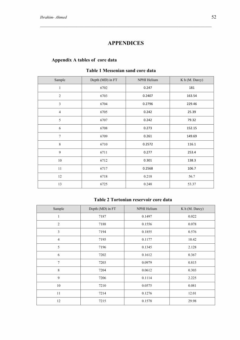
Ibrahim- Ahmed 52 _____________________________________________________________________________________

APPENDICES

Appendix A tables of core data

Table 1 Messenian sand core data

Table 2 Tortonian reservoir core data

Sample Depth (MD) in FT NPHI Helium K h (M. Darcy)

1 7187 0.1497 0.022

2 7188 0.1556 0.078

3 7194 0.1855 0.576

4 7195 0.1177 10.42

5 7196 0.1345 2.128

6 7202 0.1612 0.367

7 7203 0.0979 0.815

8 7204 0.0612 0.303

9 7206 0.1114 2.225

10 7210 0.0575 0.081

11 7214 0.1276 12.01

12 7215 0.1578 29.98


1 6702 0.247 181

2 6703 0.2407 163.54

3 6704 0.2796 229.46

4 6705 0.242 25.39

5 6707 0.242 79.32

6 6708 0.273 152.15

7 6709 0.261 149.69

8 6710 0.2572 116.1

9 6711 0.277 253.4

10 6712 0.301 138.3

11 6717 0.2568 106.7

12 6718 0.218 56.7

13 6725 0.248 53.37

Ibrahim- Ahmed 53 _____________________________________________________________________________________


13 7218 0.1621 0.361

14 7219 0.1926 0.038

15 7220 0.1862 0.853

16 7224 0.0996 0.113

17 7225 0.1639 6.658

18 7226 0.1673 0.27

19 7228 0.1451 15.138

20 7229 0.0682 0.293

Appendix B tables of well-logs

Table 3 Messenian sand (cored interval) log data.

Depth

(FT)

Gamma-ray

(API)

NPHI (neutron)

(FT3/FT3)

RHOB (density)

(g/cm3)

6702 73.03 0.2563 2.3665

6703 73.66 0.2698 2.4053

6704 69.62 0.2563 2.3873

6705 66.84 0.2654 2.3522

6707 58.75 0.4064 2.1047

6708 59.59 0.3134 2.2312

6709 62.06 0.2669 2.2711

6710 63.86 0.279 2.2946

6711 57.58 0.2724 2.3038

6712 45.11 0.2586 2.2635

6717 62.5 0.247 2.3321

6718 51.81 0.2607 2.2716

6725 82.29 0.2464 2.4491

Table 4 Tortonian sand (cored interval) log data.

Depth

(FT)

Gamma-ray

(API)

NPHI (neutron)

(FT3/FT3)

RHOB (density)

(g/cm3)

7179 61.6 0.1886 2.5376

7180 49.41 0.214 2.4314

7186 76.72 0.2322 2.5304

Ibrahim- Ahmed 54 _____________________________________________________________________________________

Depth

(FT)

Gamma-ray

(API)

NPHI (neutron)

(FT3/FT3)

RHOB (density)

(g/cm3)

7187 58.1 0.272 2.5203

7188 57.71 0.2004 2.429

7194 67.39 0.2161 2.4885

7195 65.96 0.2069 2.4334

7196 65.3 0.2171 2.4148

7198 73.45 0.2388 2.3754

7202 76.11 0.2319 2.417

7206 45.54 0.206 2.368

7207 46.62 0.213 2.4259

7210 59.72 0.2148 2.4682

7211 70.09 0.2049 2.4683

7212 78.8 0.2128 2.468

7216 69.9 0.2603 2.4982

7217 65.9 0.2053 2.4897

7218 57.75 0.2333 2.4046

7220 65.74 0.1642 2.5118

7221 83.09 0.2069 2.404

Table 5 Gamma-1 logs data for interesting intervals of Tortonian FM

Depth

FT-MD

Gamma-ray

API

Neutron

FT/FT

Density

G/cm3

Resistivity

Ohm. m

7214 102.13 0.301 2.385 3.1195

7214.5 98 0.252 2.492 3.4083

7215 84.5 0.2 2.479 3.7986

7215.5 73.44 0.184 2.448 3.9894

7216 65.13 0.171 2.431 3.881

7216.5 61.91 0.173 2.408 3.7493

7217 60 0.187 2.388 3.6168

7217.5 59.81 0.199 2.384 3.7487

7218 61.81 0.22 2.399 4.2842

7218.5 64.19 0.223 2.417 4.6341

7219 68.19 0.212 2.42 4.7212

7219.5 67.56 0.203 2.404 4.3908

Ibrahim- Ahmed 55 _____________________________________________________________________________________

Depth

FT-MD

Gamma-ray

API

Neutron

FT/FT

Density

G/cm3

Resistivity

Ohm. m

7220 65.88 0.198 2.361 3.7821

7220.5 65.44 0.207 2.337 3.6161

7221 64.94 0.212 2.355 3.5605

7221.5 66.5 0.211 2.364 3.5898

7222 69.44 0.203 2.361 3.7357

7222.5 72.31 0.203 2.341 3.6896

7223 73.19 0.203 2.339 3.4729

7223.5 68.25 0.206 2.317 3.3864

7224 70.75 0.207 2.299 3.2386

7224.5 70.94 0.205 2.312 3.0908

7225 76.75 0.193 2.336 3.3961

7225.5 76.75 0.182 2.379 3.8386

7226 81.44 0.18 2.423 4.1349

7226.5 87.13 0.201 2.483 4.4101

7227 94.38 0.217 2.487 4.3561

7227.5 96.06 0.243 2.485 4.0901

7228 89.69 0.245 2.477 3.8605

7251 106.31 0.384 2.312 2.5123

7251.5 104.5 0.286 2.415 2.8212

7252 97.5 0.217 2.464 2.9704

7252.5 92.19 0.218 2.459 2.882

7253 89.06 0.231 2.461 2.6921

7253.5 83.38 0.237 2.421 2.46

7254 73.38 0.223 2.411 2.3148

7254.5 65.25 0.213 2.406 2.327

7255 66.19 0.214 2.41 2.3278

7255.5 70.19 0.242 2.39 2.2617

7256 71.06 0.239 2.394 2.2489

7256.5 71.31 0.246 2.38 2.2474

7257 68.94 0.221 2.369 2.2638

7257.5 68.56 0.214 2.378 2.3535

7258 68 0.198 2.403 2.4343

7258.5 69.13 0.2 2.398 2.4857

Ibrahim- Ahmed 56 _____________________________________________________________________________________

Depth

FT-MD

Gamma-ray

API

Neutron

FT/FT

Density

G/cm3

Resistivity

Ohm. m

7259 66.44 0.201 2.376 2.4759

7259.5 62.03 0.205 2.363 2.4337

7260 61.69 0.21 2.35 2.3814

7260.5 66.19 0.215 2.361 2.3193

7261 63.41 0.218 2.37 2.2283

7261.5 61.72 0.217 2.352 2.2136

7262 60.47 0.206 2.338 2.2567

7262.5 65.88 0.198 2.35 2.3231

7263 68.81 0.19 2.362 2.351

7263.5 65.19 0.206 2.372 2.2007

7264 67.25 0.22 2.365 1.971

7264.5 65.19 0.237 2.347 1.8411

7265 66.88 0.232 2.319 1.7242

7265.5 64.5 0.23 2.301 1.6842

7266 66.44 0.218 2.292 1.8184

7266.5 71.56 0.21 2.307 2.0991

7267 73.38 0.196 2.351 2.4076

7267.5 73.94 0.195 2.407 2.6402

7268 75.75 0.194 2.426 2.6337

7268.5 80.25 0.205 2.423 2.4373

7269 80.19 0.201 2.399 2.1779

7269.5 77.75 0.208 2.388 2.0295

7270 71.5 0.21 2.374 1.9284

7270.5 76.38 0.214 2.376 1.8661

7271 71.56 0.209 2.38 1.8447

7271.5 73.75 0.198 2.389 1.7682

7272 66.31 0.186 2.388 1.7656

7272.5 68.63 0.202 2.38 2.1124

7273 74.88 0.213 2.387 2.3897

7511 75.94 0.255 2.472 3.4998

7511.5 69.38 0.228 2.479 3.6025

7512 69.06 0.214 2.493 3.5821

7512.5 74.94 0.2 2.483 3.2241

Ibrahim- Ahmed 57 _____________________________________________________________________________________

Depth

FT-MD

Gamma-ray

API

Neutron

FT/FT

Density

G/cm3

Resistivity

Ohm. m

7513 72.63 0.216 2.482 3.0736

7513.5 67.94 0.21 2.492 3.1141

7514 64.88 0.189 2.496 3.2713

7514.5 64.81 0.174 2.502 3.6888

7515 63.25 0.172 2.521 4.0371

7515.5 57.44 0.197 2.515 4.0889

7516 59.91 0.216 2.476 3.938

7516.5 60.19 0.215 2.448 3.4113

7517 61.09 0.224 2.436 2.9049

7517.5 57.31 0.216 2.425 2.6126

7518 62.72 0.221 2.43 2.3308

7518.5 63.5 0.2 2.43 2.2177

7519 64.13 0.207 2.428 2.2801

7519.5 61.59 0.207 2.413 2.4261

7520 62 0.211 2.428 2.7189

7520.5 64 0.208 2.454 2.8435

7521 62.31 0.205 2.458 2.8655

7521.5 63.53 0.205 2.433 3.1894

7522 64.56 0.197 2.445 3.1399

7522.5 67.31 0.203 2.476 2.9841

7523 68.5 0.22 2.472 3.0751

7523.5 68.06 0.225 2.441 2.7771

7524 68.19 0.215 2.423 2.4438

7524.5 67.31 0.213 2.42 2.3294

7525 70.31 0.214 2.417 2.3265

7525.5 67.69 0.217 2.421 2.5888

7526 67.88 0.192 2.428 2.8219

7526.5 61.97 0.189 2.452 3.1303

7527 62.34 0.207 2.465 3.7895

7527.5 58.59 0.233 2.5 4.3381

7528 61.78 0.235 2.525 4.6753

7528.5 62.88 0.227 2.532 4.6315

7529 66.44 0.223 2.517 4.5075

Ibrahim- Ahmed 58 _____________________________________________________________________________________

Depth

FT-MD

Gamma-ray

API

Neutron

FT/FT

Density

G/cm3

Resistivity

Ohm. m

7529.5 68.44 0.212 2.526 4.5397

7530 67.06 0.197 2.53 4.6486

7530.5 66.06 0.186 2.545 5.1023

7531 68.5 0.19 2.547 5.4297

7531.5 74.13 0.193 2.555 5.5579

7532 76.5 0.208 2.548 5.9196

7532.5 71.31 0.209 2.555 5.5409

7533 66.44 0.216 2.555 5.1335

7533.5 64.38 0.205 2.545 5.1673

7534 65.81 0.214 2.536 5.0675

7534.5 68.19 0.203 2.52 5.1482

7535 67.5 0.207 2.534 5.9096

7535.5 66.56 0.206 2.531 6.3249

7536 67.13 0.218 2.535 6.1143

7536.5 71.69 0.227 2.525 4.8239

7537 81.31 0.303 2.506 3.2765

7537.5 91.19 0.344 2.427 2.3126

7538 98.38 0.37 2.36 1.8094

7538.5 97.75 0.346 2.318 1.664

7539 99.94 0.365 2.281 1.7628

7539.5 94.81 0.344 2.266 2.0725

7540 91.13 0.307 2.349 2.4773

7540.5 79.13 0.254 2.385 2.66

7541 71.63 0.237 2.357 2.631

7541.5 63.59 0.231 2.331 2.4231

7542 60.31 0.232 2.328 2.1451

7542.5 64.75 0.241 2.319 2.0244

7543 66.25 0.246 2.303 2.0268

7543.5 68.13 0.243 2.268 1.9885

7544 62.5 0.24 2.251 1.86

7544.5 66.13 0.23 2.249 1.7379

7545 62.63 0.24 2.258 1.6802

7545.5 64 0.26 2.258 1.5862

Ibrahim- Ahmed 59 _____________________________________________________________________________________

Depth

FT-MD

Gamma-ray

API

Neutron

FT/FT

Density

G/cm3

Resistivity

Ohm. m

7546 62.53 0.267 2.257 1.5316

7546.5 63.44 0.255 2.252 1.5237

7547 63.5 0.247 2.246 1.5327

7547.5 67.25 0.24 2.24 1.5734

7548 72.5 0.242 2.255 1.6727

7548.5 80.63 0.234 2.269 1.725

7549 85.19 0.235 2.271 1.6677

7549.5 82.44 0.234 2.259 1.5978

7550 75.31 0.226 2.248 1.571

7550.5 69.69 0.225 2.258 1.6548

7551 76.31 0.219 2.289 1.8907

7551.5 80.06 0.222 2.332 2.2372

7552 85.19 0.225 2.366 2.369

7552.5 82.06 0.231 2.383 2.1342

7553 80.13 0.229 2.367 1.9108

7553.5 69.25 0.227 2.353 1.7391

7554 63.66 0.227 2.343 1.6438

7554.5 64.5 0.239 2.334 1.6602

7555 64.88 0.232 2.31 1.6996

7555.5 65.94 0.247 2.304 1.795

7556 62.06 0.256 2.319 1.9496

7556.5 66.13 0.254 2.339 2.0958

7557 66 0.222 2.349 2.2257

7557.5 64.88 0.221 2.343 2.2638

7558 63.66 0.219 2.327 2.1379

7558.5 64.19 0.238 2.312 2.0524

7559 67.5 0.229 2.314 2.1517

7559.5 69.13 0.237 2.344 2.3759

7560 73.63 0.23 2.376 2.7688

7560.5 79.44 0.232 2.403 3.3674

7561 84.44 0.247 2.43 3.7583

7622 112 0.33 2.41 2.23

7622.5 102.81 0.28 2.463 2.4907

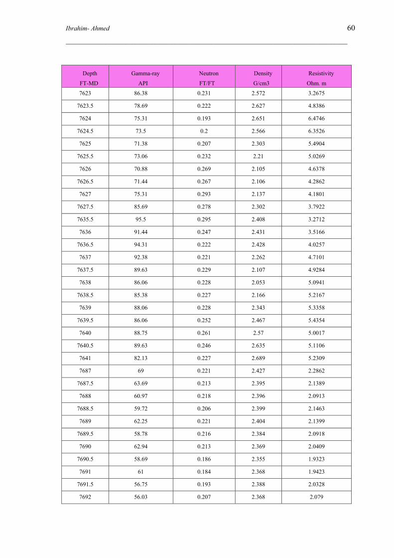
Ibrahim- Ahmed 60 _____________________________________________________________________________________

Depth

FT-MD

Gamma-ray

API

Neutron

FT/FT

Density

G/cm3

Resistivity

Ohm. m

7623 86.38 0.231 2.572 3.2675

7623.5 78.69 0.222 2.627 4.8386

7624 75.31 0.193 2.651 6.4746

7624.5 73.5 0.2 2.566 6.3526

7625 71.38 0.207 2.303 5.4904

7625.5 73.06 0.232 2.21 5.0269

7626 70.88 0.269 2.105 4.6378

7626.5 71.44 0.267 2.106 4.2862

7627 75.31 0.293 2.137 4.1801

7627.5 85.69 0.278 2.302 3.7922

7635.5 95.5 0.295 2.408 3.2712

7636 91.44 0.247 2.431 3.5166

7636.5 94.31 0.222 2.428 4.0257

7637 92.38 0.221 2.262 4.7101

7637.5 89.63 0.229 2.107 4.9284

7638 86.06 0.228 2.053 5.0941

7638.5 85.38 0.227 2.166 5.2167

7639 88.06 0.228 2.343 5.3358

7639.5 86.06 0.252 2.467 5.4354

7640 88.75 0.261 2.57 5.0017

7640.5 89.63 0.246 2.635 5.1106

7641 82.13 0.227 2.689 5.2309

7687 69 0.221 2.427 2.2862

7687.5 63.69 0.213 2.395 2.1389

7688 60.97 0.218 2.396 2.0913

7688.5 59.72 0.206 2.399 2.1463

7689 62.25 0.221 2.404 2.1399

7689.5 58.78 0.216 2.384 2.0918

7690 62.94 0.213 2.369 2.0409

7690.5 58.69 0.186 2.355 1.9323

7691 61 0.184 2.368 1.9423

7691.5 56.75 0.193 2.388 2.0328

7692 56.03 0.207 2.368 2.079

Ibrahim- Ahmed 61 _____________________________________________________________________________________

Depth

FT-MD

Gamma-ray

API

Neutron

FT/FT

Density

G/cm3

Resistivity

Ohm. m

7692.5 55.31 0.203 2.357 2.1338

7693 58.44 0.187 2.35 2.1817

7693.5 60.34 0.176 2.352 2.2759

7694 60.38 0.181 2.403 2.3619

7694.5 58.56 0.209 2.49 2.6213

7695 62.44 0.243 2.592 3.2123


Depth

FT-MD

Gamma-ray

API

Neutron

FT3/FT3

Density

G/cm3

Resistivity

Ohm. m

7201.8 53.84 0.2036 2.3372 2.2756

7202.0 51.19 0.1958 2.3263 2.2446

7202.2 48.84 0.1909 2.319 2.2524

7202.3 46.5 0.186 2.3116 2.2602

7202.5 44.16 0.1811 2.3043 2.268

7202.7 42.16 0.1818 2.2934 2.2669

7202.8 40.16 0.1825 2.2826 2.2658

7203.0 38.16 0.1832 2.2717 2.2647

7203.2 36.57 0.1892 2.2726 2.2734

7203.3 34.99 0.1952 2.2734 2.282

7203.5 33.41 0.2012 2.2742 2.2907

7203.7 33.95 0.2062 2.2772 2.299

7205.0 40.25 0.2049 2.3085 2.3185

7205.2 40.22 0.2058 2.3087 2.3116

7205.3 40.19 0.2066 2.309 2.3048

7205.5 40.16 0.2075 2.3093 2.2979

7205.7 39.93 0.2096 2.3012 2.2832

7208.2 46.67 0.2049 2.2953 2.2799

7208.3 46.11 0.1951 2.2983 2.3124

7208.5 45.56 0.1853 2.3014 2.3449

7208.7 45.75 0.1895 2.3043 2.3863

7208.8 45.94 0.1937 2.3073 2.4276

7209.0 46.13 0.198 2.3102 2.469

Ibrahim- Ahmed 62 _____________________________________________________________________________________

Depth

FT-MD

Gamma-ray

API

Neutron

FT3/FT3

Density

G/cm3

Resistivity

Ohm. m

7209.2 47.49 0.1942 2.3142 2.5354

7209.3 48.85 0.1904 2.3182 2.6018

7209.5 50.22 0.1867 2.3222 2.6681

7209.7 51.91 0.1903 2.3309 2.7576

7209.8 53.59 0.194 2.3396 2.8472

7210.0 55.28 0.1976 2.3482 2.9367

7210.2 56.61 0.1935 2.3579 2.9904

7210.3 57.95 0.1894 2.3676 3.0442

7210.5 59.28 0.1853 2.3773 3.0979

7210.7 59.52 0.1815 2.3853 3.132

7210.8 59.76 0.1778 2.3933 3.1661

7211.0 60 0.1741 2.4013 3.2002

7211.2 61.79 0.1697 2.4039 3.2343

7211.3 63.58 0.1653 2.4065 3.2684

7211.5 65.38 0.1609 2.4091 3.3025

7211.7 67.27 0.1646 2.4154 3.3877

7211.8 69.17 0.1682 2.4216 3.4729

7212.0 71.06 0.1719 2.4279 3.5581

7218.0 48.84 0.2158 2.4303 3.915

7218.2 49.27 0.2089 2.4221 3.9197

7218.3 49.7 0.2019 2.4139 3.9244

7218.5 50.13 0.1949 2.4057 3.9291

7218.7 51.31 0.1864 2.4049 3.9488

7218.8 52.5 0.1778 2.4042 3.9686

7219.0 53.69 0.1693 2.4034 3.9883

7219.2 54.24 0.1675 2.408 4.0259

7219.3 54.79 0.1658 2.4126 4.0635

7219.5 55.34 0.164 2.4173 4.101

7219.7 53.53 0.166 2.4295 3.9196

7219.8 51.72 0.168 2.4417 3.7382

7220.0 49.91 0.1699 2.4539 3.5568

7223.0 57.91 0.2022 2.5251 4.7745

7223.2 57.7 0.1989 2.528 4.8709

7223.3 57.49 0.1955 2.5309 4.9673

Ibrahim- Ahmed 63 _____________________________________________________________________________________

Depth

FT-MD

Gamma-ray

API

Neutron

FT3/FT3

Density

G/cm3

Resistivity

Ohm. m

7223.5 57.28 0.1921 2.5338 5.0637

7223.7 54.67 0.1895 2.5233 4.8735

7223.8 52.05 0.1869 2.5127 4.6832

7224.0 49.44 0.1844 2.5022 4.493

7224.2 49.56 0.1783 2.4815 4.2812

7224.3 49.69 0.1723 2.4608 4.0693

7224.5 49.81 0.1662 2.44 3.8575

7224.7 48.95 0.1723 2.4306 3.771

7224.8 48.08 0.1785 2.4211 3.6844

7225.0 47.22 0.1846 2.4116 3.5979

7225.2 47.31 0.186 2.4039 3.5536

7225.3 47.41 0.1874 2.3962 3.5093

7225.5 47.5 0.1887 2.3884 3.4651

7225.7 47.6 0.193 2.3935 3.421

7225.8 47.71 0.1972 2.3987 3.3769

7226.0 47.81 0.2015 2.4038 3.3328

7226.2 48.8 0.1971 2.4065 3.3716

7226.3 49.79 0.1927 2.4093 3.4104

7226.5 50.78 0.1882 2.4121 3.4492

7226.7 51.18 0.2011 2.4196 3.3938

7226.8 51.57 0.214 2.4271 3.3384

7288.2 30.18 0.2084 2.3801 2.5151

7288.3 30.55 0.2064 2.3727 2.5047

7288.5 30.92 0.2045 2.3653 2.4942

7288.7 30.3 0.1981 2.3698 2.5088

7288.8 29.68 0.1916 2.3744 2.5234

7289.0 29.06 0.1851 2.3789 2.5379

7289.2 29.9 0.1852 2.3837 2.559

7289.3 30.73 0.1853 2.3885 2.5801

7289.5 31.56 0.1854 2.3933 2.6012

7289.7 31.73 0.1845 2.3934 2.6091

7289.8 31.9 0.1835 2.3934 2.617

7290.0 32.06 0.1826 2.3935 2.6249

7290.2 33.76 0.1884 2.3961 2.6915

Ibrahim- Ahmed 64 _____________________________________________________________________________________

Depth

FT-MD

Gamma-ray

API

Neutron

FT3/FT3

Density

G/cm3

Resistivity

Ohm. m

7290.3 35.46 0.1942 2.3987 2.7582

7290.5 37.16 0.1999 2.4013 2.8249

7290.7 40.39 0.1972 2.4016 2.9418

7290.8 43.61 0.1945 2.402 3.0587

7291.0 46.84 0.1917 2.4023 3.1756

7291.2 50.93 0.1997 2.4128 3.2879

7291.3 55.01 0.2077 2.4233 3.4003

7314.0 59.59 0.2177 2.4188 3.3718

7314.2 56.97 0.2137 2.419 3.2559

7314.3 54.34 0.2097 2.4193 3.14

7314.5 51.72 0.2056 2.4195 3.0241

7314.7 51.29 0.2084 2.4154 2.9407

7314.8 50.86 0.2112 2.4114 2.8574

7315.0 50.44 0.2141 2.4074 2.774

7315.2 49.07 0.2219 2.3937 2.7566

7315.3 47.71 0.2298 2.3801 2.7393

7315.5 46.34 0.2377 2.3664 2.7219

7315.7 48.14 0.2355 2.3595 2.727

7315.8 49.93 0.2333 2.3525 2.7321

7316.0 51.72 0.2311 2.3456 2.7372

7316.2 52.64 0.2319 2.3508 2.7901

7316.3 53.55 0.2328 2.3559 2.8431

7316.5 54.47 0.2336 2.3611 2.896

7316.7 57.03 0.258 2.3685 3.0472

7316.8 59.59 0.2823 2.376 3.1984

7317.0 62.16 0.3067 2.3835 3.3496

Table 7 Gamma-3 log data for interesting intervals of Tortonian FM

Depth

FT-MD

Gamma-ray

API

Neutron

FT3/FT3

Density

G/cm3

Resistivity

Ohm. m

7046.0 36.0 0.022 2.385 10.5

7046.2 35.3 0.036 2.358 9.3

7046.3 34.6 0.050 2.331 8.0

7046.5 33.9 0.064 2.303 6.8

Ibrahim- Ahmed 65 _____________________________________________________________________________________

Depth

FT-MD

Gamma-ray

API

Neutron

FT3/FT3

Density

G/cm3

Resistivity

Ohm. m

7046.7 34.0 0.091 2.312 6.1

7046.8 34.1 0.118 2.320 5.4

7047.0 34.2 0.145 2.328 4.7

7047.2 34.1 0.174 2.339 4.4

7047.3 33.9 0.202 2.349 4.1

7050.2 35.4 0.184 2.471 12.2

7050.3 34.0 0.149 2.541 12.8

7050.5 32.7 0.114 2.612 13.5

7050.7 32.1 0.098 2.636 12.6

7050.8 31.4 0.083 2.661 11.8

7051.0 30.8 0.067 2.685 11.0

7051.2 31.1 0.073 2.687 10.7

7051.3 31.5 0.079 2.689 10.3

7051.5 31.8 0.086 2.692 10.0

7051.7 32.6 0.083 2.687 9.9

7051.8 33.4 0.081 2.683 9.7

7052.0 34.3 0.079 2.679 9.5

7052.2 33.9 0.082 2.667 9.3

7052.3 33.5 0.085 2.656 9.1

7052.5 33.2 0.088 2.644 8.9

7052.7 32.0 0.095 2.595 8.7

7052.8 30.9 0.103 2.545 8.5

7053.0 29.7 0.110 2.495 8.3

7053.2 29.4 0.125 2.472 8.3

7053.3 29.0 0.139 2.449 8.2

7053.5 28.7 0.154 2.427 8.2

7053.7 28.1 0.158 2.425 8.4

7053.8 27.6 0.163 2.423 8.6

7054.0 27.0 0.168 2.421 8.8

7054.2 27.1 0.163 2.445 8.8

7054.3 27.1 0.158 2.469 8.8

7054.5 27.2 0.153 2.493 8.8

7054.7 27.2 0.149 2.432 8.7

7054.8 27.3 0.145 2.372 8.6

Ibrahim- Ahmed 66 _____________________________________________________________________________________

Depth

FT-MD

Gamma-ray

API

Neutron

FT3/FT3

Density

G/cm3

Resistivity

Ohm. m

7055.0 27.3 0.141 2.311 8.6

7055.2 27.6 0.151 2.261 8.7

7055.3 28.0 0.161 2.210 8.8

7055.5 28.3 0.171 2.160 8.9

7055.7 28.5 0.184 2.141 9.4

7055.8 28.7 0.197 2.123 9.9

7056.0 28.9 0.210 2.105 10.3

7056.2 28.3 0.203 2.153 11.3

7056.3 27.7 0.196 2.201 12.3

7056.5 27.1 0.189 2.249 13.3

7056.7 26.7 0.164 2.322 14.0

7056.8 26.3 0.139 2.395 14.7

7057.0 25.9 0.114 2.467 15.5

7057.2 25.5 0.090 2.544 16.7

7057.3 25.1 0.066 2.620 17.9

7057.5 24.7 0.041 2.696 19.2

7057.7 24.8 0.035 2.705 21.3

7057.8 24.9 0.029 2.714 23.5

7058.0 25.1 0.023 2.722 25.6

7058.2 25.4 0.023 2.711 25.2

7058.3 25.7 0.023 2.700 24.8

7058.5 26.1 0.023 2.689 24.5

7058.7 26.2 0.022 2.694 25.3

7058.8 26.4 0.021 2.698 26.2

7059.0 26.5 0.020 2.702 27.1

7059.2 26.7 0.019 2.701 26.8

7059.3 26.9 0.018 2.700 26.6

7059.5 27.1 0.017 2.699 26.3

7059.7 27.5 0.017 2.697 26.5

7059.8 28.0 0.017 2.696 26.8

7060.0 28.4 0.017 2.695 27.0

7060.2 27.9 0.017 2.689 28.7

7060.3 27.5 0.016 2.684 30.4

7060.5 27.0 0.016 2.678 32.1

Ibrahim- Ahmed 67 _____________________________________________________________________________________

Depth

FT-MD

Gamma-ray

API

Neutron

FT3/FT3

Density

G/cm3

Resistivity

Ohm. m

7060.7 26.6 0.015 2.682 34.5

7060.8 26.1 0.014 2.685 37.0

7061.0 25.7 0.013 2.689 39.4

7061.2 25.0 0.011 2.693 39.8

7061.3 24.2 0.010 2.698 40.2

7061.5 23.5 0.008 2.703 40.6

7061.7 25.0 0.008 2.705 37.8

7061.8 26.4 0.008 2.707 35.0

7062.0 27.8 0.008 2.708 32.1

7062.2 28.9 0.009 2.706 27.8

7062.3 29.9 0.010 2.705 23.5

7062.5 30.9 0.010 2.703 19.1

7062.7 31.4 0.016 2.691 17.3

7062.8 31.9 0.022 2.679 15.5

7063.0 32.4 0.028 2.667 13.6

7063.2 31.4 0.034 2.662 13.6

7063.3 30.4 0.040 2.657 13.5

7063.5 29.4 0.045 2.653 13.4

7063.7 28.0 0.049 2.664 13.9

7063.8 26.6 0.053 2.675 14.4

7064.0 25.1 0.057 2.687 14.8

7064.2 25.6 0.051 2.699 15.4

7064.3 26.2 0.046 2.711 16.0

7064.5 26.7 0.041 2.722 16.6

7064.7 26.4 0.038 2.715 16.8

7064.8 26.2 0.035 2.707 17.0

7065.0 25.9 0.031 2.699 17.2

7065.2 26.3 0.031 2.694 16.8

7065.3 26.6 0.030 2.689 16.4

7065.5 27.0 0.030 2.684 16.0

7065.7 26.7 0.029 2.678 15.8

7065.8 26.4 0.029 2.672 15.6

7066.0 26.1 0.029 2.665 15.4

7066.2 26.5 0.032 2.661 14.8

Ibrahim- Ahmed 68 _____________________________________________________________________________________

Depth

FT-MD

Gamma-ray

API

Neutron

FT3/FT3

Density

G/cm3

Resistivity

Ohm. m

7066.3 26.9 0.036 2.658 14.1

7066.5 27.3 0.039 2.654 13.5

7066.7 29.1 0.041 2.633 12.7

7066.8 30.8 0.044 2.612 11.9

7067.0 32.5 0.046 2.591 11.0

7067.2 33.1 0.057 2.570 10.7

7067.3 33.8 0.067 2.548 10.4

7067.5 34.5 0.078 2.526 10.0

7067.7 35.2 0.092 2.499 10.0

7067.8 35.9 0.106 2.473 10.0

7068.0 36.6 0.120 2.446 10.0

7068.2 35.1 0.134 2.446 10.2

7068.3 33.6 0.149 2.446 10.4

7068.5 32.0 0.163 2.445 10.7

7068.7 31.6 0.163 2.443 11.0

7068.8 31.1 0.163 2.441 11.4

7069.0 30.6 0.163 2.439 11.8

7069.2 29.2 0.154 2.451 12.5

7069.3 27.8 0.146 2.462 13.2

7069.5 26.3 0.137 2.474 13.9

7069.7 26.6 0.128 2.498 14.3

7069.8 26.9 0.119 2.522 14.7

7070.0 27.1 0.110 2.546 15.1

7070.2 26.9 0.110 2.552 15.6

7070.3 26.7 0.109 2.558 16.0

7070.5 26.5 0.109 2.564 16.4

7070.7 27.1 0.108 2.572 16.3

7070.8 27.7 0.107 2.580 16.1

7071.0 28.2 0.106 2.588 15.9

7071.2 28.2 0.104 2.601 14.9

7071.3 28.2 0.102 2.615 13.9

7071.5 28.2 0.100 2.629 12.9

7071.7 29.0 0.090 2.606 12.1

7071.8 29.8 0.080 2.584 11.3

Ibrahim- Ahmed 69 _____________________________________________________________________________________

Depth

FT-MD

Gamma-ray

API

Neutron

FT3/FT3

Density

G/cm3

Resistivity

Ohm. m

7072.0 30.5 0.070 2.561 10.5

7072.2 30.6 0.070 2.514 10.0

7072.3 30.7 0.069 2.467 9.6

7072.5 30.8 0.069 2.421 9.1

7072.7 30.8 0.077 2.415 8.8

7072.8 30.8 0.085 2.410 8.6

7073.0 30.8 0.094 2.404 8.3

7073.2 30.7 0.111 2.434 8.5

7073.3 30.6 0.129 2.463 8.6

7073.5 30.5 0.146 2.492 8.8

7073.7 30.7 0.150 2.492 9.4

7073.8 30.9 0.153 2.491 9.9

7074.0 31.1 0.157 2.490 10.5

7074.2 31.4 0.147 2.500 11.8

7074.3 31.6 0.137 2.510 13.0

7074.5 31.9 0.127 2.520 14.2

7074.7 30.7 0.109 2.546 16.6

7074.8 29.6 0.091 2.572 18.9

7075.0 28.4 0.072 2.598 21.3

7075.2 27.9 0.057 2.636 26.9

7075.3 27.4 0.041 2.673 32.5

7075.5 26.9 0.026 2.710 38.1

7075.7 26.5 0.020 2.717 39.5

7075.8 26.0 0.015 2.723 41.0

7076.0 25.6 0.010 2.730 42.4

7076.2 26.6 0.009 2.724 38.8

7076.3 27.6 0.009 2.719 35.2

7076.5 28.6 0.008 2.713 31.7

7076.7 28.5 0.010 2.708 28.5

7076.8 28.3 0.012 2.703 25.4

7077.0 28.2 0.014 2.698 22.3

7077.2 29.2 0.016 2.695 20.0

7077.3 30.3 0.019 2.692 17.7

7077.5 31.3 0.021 2.690 15.4

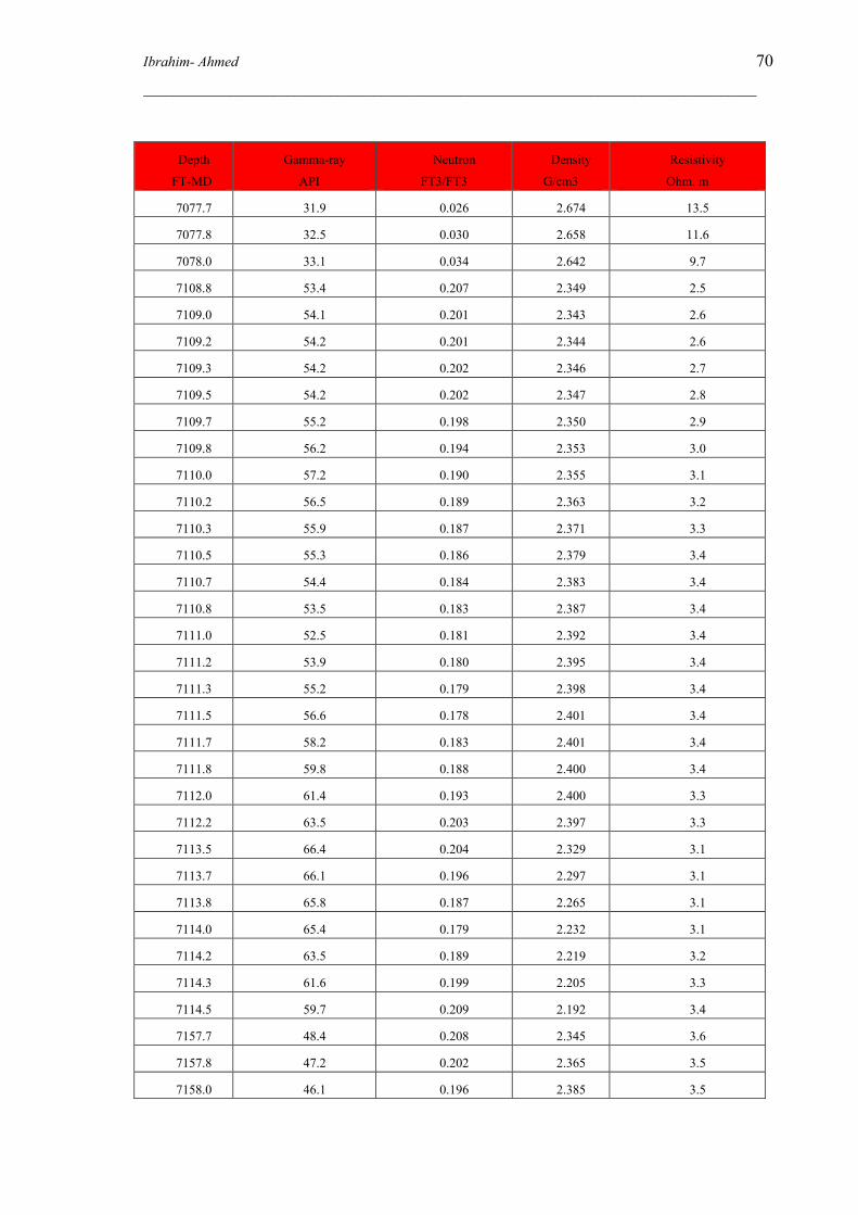
Ibrahim- Ahmed 70 _____________________________________________________________________________________

Depth

FT-MD

Gamma-ray

API

Neutron

FT3/FT3

Density

G/cm3

Resistivity

Ohm. m

7077.7 31.9 0.026 2.674 13.5

7077.8 32.5 0.030 2.658 11.6

7078.0 33.1 0.034 2.642 9.7

7108.8 53.4 0.207 2.349 2.5

7109.0 54.1 0.201 2.343 2.6

7109.2 54.2 0.201 2.344 2.6

7109.3 54.2 0.202 2.346 2.7

7109.5 54.2 0.202 2.347 2.8

7109.7 55.2 0.198 2.350 2.9

7109.8 56.2 0.194 2.353 3.0

7110.0 57.2 0.190 2.355 3.1

7110.2 56.5 0.189 2.363 3.2

7110.3 55.9 0.187 2.371 3.3

7110.5 55.3 0.186 2.379 3.4

7110.7 54.4 0.184 2.383 3.4

7110.8 53.5 0.183 2.387 3.4

7111.0 52.5 0.181 2.392 3.4

7111.2 53.9 0.180 2.395 3.4

7111.3 55.2 0.179 2.398 3.4

7111.5 56.6 0.178 2.401 3.4

7111.7 58.2 0.183 2.401 3.4

7111.8 59.8 0.188 2.400 3.4

7112.0 61.4 0.193 2.400 3.3

7112.2 63.5 0.203 2.397 3.3

7113.5 66.4 0.204 2.329 3.1

7113.7 66.1 0.196 2.297 3.1

7113.8 65.8 0.187 2.265 3.1

7114.0 65.4 0.179 2.232 3.1

7114.2 63.5 0.189 2.219 3.2

7114.3 61.6 0.199 2.205 3.3

7114.5 59.7 0.209 2.192 3.4

7157.7 48.4 0.208 2.345 3.6

7157.8 47.2 0.202 2.365 3.5

7158.0 46.1 0.196 2.385 3.5

Ibrahim- Ahmed 71 _____________________________________________________________________________________

Depth

FT-MD

Gamma-ray

API

Neutron

FT3/FT3

Density

G/cm3

Resistivity

Ohm. m

7158.2 45.7 0.193 2.391 3.4

7158.3 45.3 0.190 2.397 3.4

7158.5 44.8 0.187 2.404 3.3

7158.7 45.8 0.187 2.407 3.3

7158.8 46.8 0.187 2.410 3.3

7159.0 47.8 0.186 2.413 3.3

7159.2 49.1 0.186 2.414 3.3

7159.3 50.4 0.187 2.416 3.3

7159.5 51.7 0.187 2.417 3.3

7159.7 52.1 0.192 2.414 3.2

7159.8 52.6 0.196 2.412 3.1

7160.0 53.0 0.201 2.409 3.0

7160.2 52.8 0.206 2.410 3.0

7161.2 56.3 0.210 2.417 2.7

7161.3 57.3 0.206 2.412 2.6

7161.5 58.4 0.202 2.408 2.6

7161.7 60.7 0.203 2.402 2.5

7161.8 63.0 0.204 2.396 2.4

7162.0 65.4 0.204 2.390 2.3


Depth

FT-MD

Gamma-ray

API

Neutron

FT3/FT3

Density

G/cm3

Resistivity

Ohm. m

7173.0 80.59 0.3259 2.2774 1.7224

7173.2 80 0.3299 2.237 1.7298

7173.3 79.41 0.3339 2.1967 1.7371

7173.5 78.82 0.3379 2.1564 1.7445

7173.7 73.73 0.3535 2.1313 1.7431

7173.8 68.63 0.3691 2.1062 1.7417

7174.0 63.54 0.3847 2.0812 1.7402

7174.2 63.21 0.402 2.1089 1.7812

7174.3 62.87 0.4192 2.1366 1.8222

7174.5 62.54 0.4364 2.1643 1.8632

7174.7 62.29 0.4211 2.2188 1.9611

Ibrahim- Ahmed 72 _____________________________________________________________________________________

Depth

FT-MD

Gamma-ray

API

Neutron

FT3/FT3

Density

G/cm3

Resistivity

Ohm. m

7174.8 62.05 0.4059 2.2733 2.0589

7175.0 61.8 0.3906 2.3278 2.1567

7175.2 61.63 0.3616 2.3634 2.2766

7175.3 61.45 0.3327 2.3989 2.3965

7175.5 61.28 0.3037 2.4345 2.5163

7175.7 61.01 0.2783 2.4511 2.6284

7175.8 60.75 0.2529 2.4678 2.7405

7176.0 60.48 0.2275 2.4844 2.8526

7176.2 59.61 0.2185 2.4991 3.0071

7176.3 58.75 0.2094 2.5138 3.1615

7176.5 57.88 0.2004 2.5286 3.316

7176.7 57.81 0.1968 2.5517 3.63

7176.8 57.73 0.1932 2.5749 3.944

7177.0 57.66 0.1897 2.5981 4.258

7177.2 59.28 0.1871 2.6126 4.6332

7177.3 60.89 0.1845 2.6271 5.0083

7177.5 62.51 0.182 2.6416 5.3834

7177.7 62.99 0.1764 2.6411 5.2806

7177.8 63.47 0.1709 2.6406 5.1777

7178.0 63.95 0.1653 2.6401 5.0748

7178.2 63.95 0.1675 2.6277 4.6049

7178.3 63.94 0.1696 2.6152 4.1349

7178.5 63.94 0.1718 2.6028 3.6649

7178.7 63.16 0.1774 2.581 3.2957

7178.8 62.38 0.183 2.5593 2.9266

7179.0 61.6 0.1886 2.5376 2.5574

7179.2 57.46 0.1965 2.5151 2.5374

7179.3 53.32 0.2045 2.4926 2.5174

7179.5 49.18 0.2124 2.4701 2.4975

7179.7 49.26 0.2129 2.4572 2.5202

7179.8 49.33 0.2135 2.4443 2.543

7180.0 49.41 0.214 2.4314 2.5657

7180.2 50.39 0.2166 2.432 2.6148

7180.3 51.37 0.2192 2.4326 2.6639

Ibrahim- Ahmed 73 _____________________________________________________________________________________

Depth

FT-MD

Gamma-ray

API

Neutron

FT3/FT3

Density

G/cm3

Resistivity

Ohm. m

7180.5 52.35 0.2218 2.4332 2.713

7180.7 53.16 0.2173 2.4435 2.6824

7180.8 53.98 0.2128 2.4538 2.6518

7181.0 54.79 0.2083 2.4641 2.6212

7181.2 55.54 0.2073 2.4715 2.5477

7181.3 56.29 0.2062 2.479 2.4742

7181.5 57.04 0.2052 2.4865 2.4007

7181.7 57.79 0.2014 2.4814 2.335

7181.8 58.53 0.1975 2.4764 2.2694

7182.0 59.28 0.1937 2.4713 2.2038

7182.2 60.41 0.2012 2.4607 2.1267

7182.3 61.55 0.2086 2.4501 2.0496

7182.5 62.68 0.2161 2.4395 1.9725

7182.7 64.86 0.2215 2.4302 1.9534

7182.8 67.03 0.2268 2.421 1.9343

7183.0 69.21 0.2321 2.4117 1.9153

7203.0 77.13 0.2504 2.5324 3.6405

7203.2 75.89 0.2499 2.5262 3.6008

7203.3 74.65 0.2494 2.5199 3.5611

7203.5 73.41 0.2489 2.5137 3.5215

7203.7 70.53 0.2453 2.5049 3.3232

7203.8 67.66 0.2417 2.4962 3.1249

7204.0 64.78 0.238 2.4874 2.9267

7204.2 61.8 0.2314 2.4694 2.7856

7204.3 58.82 0.2249 2.4515 2.6445

7204.5 55.84 0.2183 2.4335 2.5034

7204.7 53.2 0.2164 2.4192 2.4016

7204.8 50.55 0.2146 2.4049 2.2999

7205.0 47.91 0.2128 2.3906 2.1981

7205.2 47.12 0.2105 2.3801 2.1149

7205.3 46.33 0.2083 2.3696 2.0318

7205.5 45.54 0.206 2.3591 1.9486

7205.7 45.54 0.206 2.3621 1.9539

7205.8 45.54 0.206 2.365 1.9592

Ibrahim- Ahmed 74 _____________________________________________________________________________________

Depth

FT-MD

Gamma-ray

API

Neutron

FT3/FT3

Density

G/cm3

Resistivity

Ohm. m

7206.0 45.54 0.206 2.368 1.9646

7206.2 45.57 0.204 2.377 2.0226

7206.3 45.61 0.202 2.386 2.0807

7206.5 45.64 0.2 2.395 2.1388

7206.7 45.97 0.2043 2.4053 2.256

7206.8 46.29 0.2087 2.4156 2.3733

7207.0 46.62 0.213 2.4259 2.4905

7207.2 48.21 0.2138 2.4286 2.6665

7207.3 49.8 0.2146 2.4312 2.8425

7207.5 51.39 0.2154 2.4339 3.0184

7207.7 54.08 0.2155 2.435 3.1497

7207.8 56.77 0.2157 2.436 3.281

7208.0 59.46 0.2159 2.4371 3.4123

7297.0 40.52 0.2 2.3351 1.2881

7297.2 42.97 0.1961 2.3411 1.2942

7297.3 45.41 0.1922 2.347 1.3004

7297.5 47.86 0.1883 2.3529 1.3065

7297.7 49.74 0.1928 2.3555 1.3103

7297.8 51.63 0.1974 2.3582 1.314

7298.0 53.51 0.2019 2.3608 1.3177

7298.2 54.86 0.2028 2.3565 1.289

7298.3 56.22 0.2038 2.3521 1.2603

7298.5 57.57 0.2047 2.3478 1.2316

7298.7 59.37 0.2065 2.3422 1.2014

7298.8 61.16 0.2083 2.3367 1.1712

7299.0 62.96 0.2101 2.3311 1.141

7299.2 64.76 0.2077 2.3312 1.15

7299.3 66.55 0.2052 2.3312 1.159

7299.5 68.35 0.2028 2.3313 1.1681

7299.7 70.15 0.1997 2.3315 1.2242

7299.8 71.94 0.1965 2.3317 1.2803

7300.0 73.74 0.1934 2.3319 1.3365

7300.2 75.54 0.1923 2.3391 1.4726

7300.3 77.33 0.1912 2.3464 1.6087

Ibrahim- Ahmed 75 _____________________________________________________________________________________

Depth

FT-MD

Gamma-ray

API

Neutron

FT3/FT3

Density

G/cm3

Resistivity

Ohm. m

7300.5 79.13 0.1901 2.3536 1.7448

7300.7 80.55 0.1959 2.3701 1.9556

Appendix C tables of results

Table 9 FZI and its relevant log data of Gamma-EX

Gamma-ray

API

Neutron

FT3/FT3

Density

G/cm3

FZI (original)

𝜇𝜇𝜇𝜇

73.03 0.2563 2.3665 2.591304694

73.66 0.2698 2.4053 2.581908868

69.62 0.2563 2.3873 2.317667315

66.84 0.2654 2.3522 1.007412082

58.75 0.4064 2.1047 1.780603233

59.59 0.3134 2.2312 1.974040537

62.06 0.2669 2.2711 2.129166967

63.86 0.279 2.2946 1.926687176

57.58 0.2724 2.3038 2.478857703

45.11 0.2586 2.2635 1.563033083

62.5 0.247 2.3321 1.852358445

51.81 0.2607 2.2716 1.816532575

82.29 0.2464 2.4491 1.396749642

61.6 0.1886 2.5376 0.068372344

49.41 0.214 2.4314 0.120645405

76.72 0.2322 2.5304 0.242949555

58.1 0.272 2.5203 2.214700953

57.71 0.2004 2.429 0.803709507

67.39 0.2161 2.4885 0.24653214

65.96 0.2069 2.4334 0.834812796

65.3 0.2171 2.4148 1.071758435

73.45 0.2388 2.3754 1.11936875

76.11 0.2319 2.417 0.610874152

45.54 0.206 2.368 2.082767523

46.62 0.213 2.4259 2.30993735

Ibrahim- Ahmed 76 _____________________________________________________________________________________

Gamma-ray

API

Neutron

FT3/FT3

Density

G/cm3

FZI (original)

𝜇𝜇𝜇𝜇

59.72 0.2148 2.4682 0.242214934

70.09 0.2049 2.4683 0.058469014

78.8 0.2128 2.468 0.293732725

69.9 0.2603 2.4982 0.302353742

65.9 0.2053 2.4897 1.020919118

57.75 0.2333 2.4046 0.198543733

65.74 0.1642 2.5118 1.889635751

83.09 0.2069 2.404 0.889220779

Table 10 FZI, effective porosity, and permeability logs of Gamma-1

Depth

FT-MD

FZI

µm

Effective Porosity

FT3/FT3

Permeability

mD

7254 1.1012 0.1179 2.0457

7254.5 1.3768 0.1363 4.9565

7255 1.3402 0.1336 4.4185

7255.5 1.2532 0.1408 4.5346

7256 1.2156 0.136 3.8442

7256.5 1.2316 0.1419 4.483

7257 1.3078 0.1398 4.8311

7257.5 1.3029 0.1354 4.355

7258 1.2756 0.1236 3.1644

7258.5 1.2456 0.1228 2.9591

7259 1.3678 0.1353 4.7915

7259.5 1.5386 0.1501 8.3026

7260 1.5719 0.1562 9.784

7260.5 1.4076 0.1459 6.373

7261 1.4925 0.1513 8.0138

7261.5 1.5736 0.1588 10.3123

7262 1.6266 0.1597 11.2153

7262.5 1.4199 0.1416 5.9276

7263 1.2973 0.1279 3.626

7263.5 1.4197 0.1415 5.9085

7264 1.37 0.1446 5.8753

7264.5 1.4779 0.1615 9.5803

Ibrahim- Ahmed 77 _____________________________________________________________________________________

Depth

FT-MD

FZI

µm

Effective Porosity

FT3/FT3

Permeability

mD

7265 1.4546 0.162 9.3765

7265.5 1.5584 0.1711 12.6971

7266 1.4953 0.1633 10.1514

7266.5 1.2941 0.1426 5.0316

7267 1.1617 0.1203 2.4184

7270 1.2052 0.1266 3.0372

7270.5 1.0396 0.1127 1.5882

7271 1.1941 0.1245 2.8353

7271.5 1.0988 0.1109 1.6888

7272 1.344 0.126 3.7223

7272.5 1.2887 0.1294 3.709

7275.5 0.7694 0.0889 0.4254

7276 1.0171 0.1283 2.2538

7276.5 1.2385 0.1552 5.9622

7277 1.3705 0.1863 12.7682

7290 1.0698 0.1668 5.5359

7290.5 0.9921 0.1569 3.9524

7294.5 1.119 0.1525 4.6139

7295 1.1098 0.1463 3.9984

7295.5 1.0008 0.1055 1.2043

7296 1.0655 0.1065 1.405

7296.5 1.2586 0.1363 4.1435

7297 1.2726 0.1511 5.7934

7307 1.1066 0.1185 2.0971

7307.5 1.2402 0.1286 3.3758

7308 1.2952 0.1323 4.0093

7308.5 1.5746 0.151 8.8576

7309 1.6612 0.1583 11.3749

7309.5 1.8296 0.1723 17.8914

7310 1.6654 0.1645 12.8667

7310.5 1.4469 0.1523 7.6735

7315 0.4989 0.0251 0.004

7511 0.9561 0.1094 1.2268

7511.5 1.1489 0.1151 2.0703

Ibrahim- Ahmed 78 _____________________________________________________________________________________

Depth

FT-MD

FZI

µm

Effective Porosity

FT3/FT3

Permeability

mD

7515.5 1.4821 0.1184 3.7478

7516 1.466 0.1319 5.0859

7516.5 1.4937 0.1377 6.0159

7517 1.4862 0.1428 6.6642

7517.5 1.6236 0.1489 9.0326

7518 1.4366 0.1396 5.8105

7518.5 1.3936 0.1285 4.2502

7519 1.3805 0.1308 4.3981

7519.5 1.4871 0.1398 6.2445

7520 1.456 0.1371 5.6466

7520.5 1.3502 0.1252 3.6867

7521 1.3999 0.1265 4.0875

7521.5 1.3924 0.13 4.3903

7522 1.3347 0.1212 3.263

7522.5 1.2036 0.1099 1.9737

7523 1.182 0.1155 2.2134

7523.5 1.2429 0.1264 3.2145

7524 1.2553 0.1259 3.2429

7524.5 1.2876 0.128 3.581

7525 1.1903 0.1213 2.6034

7525.5 1.2766 0.1286 3.5724

7526 1.2411 0.1152 2.4183

7526.5 1.4072 0.1215 3.6517

7527 1.3909 0.1256 3.9525

7527.5 1.4913 0.1362 5.7994

7528 1.3504 0.1249 3.6565

7528.5 1.2974 0.1173 2.7928

7529 1.1933 0.1111 2.0049

7530 1.134 0.0947 1.1188

7541 1.2452 0.1425 4.6445

7541.5 1.5492 0.1662 11.4983

7542 1.6658 0.1741 15.3223

7542.5 1.534 0.1711 12.3093

7543 1.5086 0.1737 12.4774

Ibrahim- Ahmed 79 _____________________________________________________________________________________

Depth

FT-MD

FZI

µm

Effective Porosity

FT3/FT3

Permeability

mD

7543.5 1.49 0.1762 12.7183

7544 1.7023 0.192 21.5899

7544.5 1.5738 0.1799 15.1123

7545 1.6885 0.19 20.5831

7545.5 1.6573 0.1961 21.8369

7546 1.7142 0.2026 25.8481

7546.5 1.6807 0.1965 22.6085

7547 1.6805 0.1942 21.8046

7547.5 1.5555 0.1839 15.7836

7548 1.3579 0.1669 8.9431

7548.5 1.056 0.132 2.6474

7550 1.2592 0.1526 5.8524

7550.5 1.4363 0.1665 9.926

7551 1.1639 0.1362 3.5373

7551.5 0.9801 0.1135 1.4447

7553.5 1.3236 0.1455 5.5946

7554 1.5277 0.1614 10.2153

7554.5 1.5206 0.1671 11.2562

7555 1.535 0.1689 11.8559

7555.5 1.5187 0.1747 12.8564

7556 1.6372 0.1836 17.4168

7556.5 1.4702 0.1689 10.8719

7557 1.4358 0.1524 7.5724

7557.5 1.4815 0.156 8.6579

7558 1.5432 0.1617 10.4779

7558.5 1.5603 0.1727 13.1037

7559 1.4378 0.1604 8.8743

7559.5 1.348 0.1525 6.6958

7564 0.6332 0.1126 0.5872

7652 1.114 0.1005 1.29

7652.5 1.2155 0.1148 2.2991

7653 1.1294 0.1064 1.5767

7653.5 1.2407 0.1186 2.6414

7654 1.3159 0.1268 3.6377

Ibrahim- Ahmed 80 _____________________________________________________________________________________

Depth

FT-MD

FZI

µm

Effective Porosity

FT3/FT3

Permeability

mD

7654.5 1.3414 0.135 4.5703

7655 1.1927 0.1251 2.8665

7655.5 1.0922 0.1204 2.1396

7656 1.1087 0.1254 2.4951

7656.5 1.2271 0.1391 4.1878

7657 1.3108 0.1419 5.0809

7657.5 1.2481 0.133 3.7842

7658 1.3995 0.1449 6.1778

7658.5 1.5271 0.1535 8.7579

7659 1.7626 0.1675 15.2251

7659.5 1.7484 0.1666 14.742

7660 1.6341 0.1593 11.2359

7660.5 1.535 0.1562 9.3358

7661 1.4275 0.1449 6.4253

7661.5 1.3958 0.1401 5.5411

7662 1.4762 0.1436 6.6863

7662.5 1.6273 0.1533 9.9016

7663 1.6598 0.1639 12.6489

7663.5 1.5443 0.1661 11.4058

7664 1.302 0.1524 6.228

7664.5 1.241 0.1451 4.8697

7665 1.2079 0.1346 3.6734

7665.5 1.2308 0.1329 3.6667

7666 1.3708 0.1408 5.4308

7666.5 1.3492 0.1418 5.3733

7667 1.3694 0.147 6.1742

7667.5 1.2478 0.1389 4.3123

7668 1.283 0.1428 4.9623

7668.5 1.1523 0.1337 3.2736

7669 1.2607 0.1473 5.2625

7669.5 1.1465 0.1362 3.4339

7670 1.2594 0.1406 4.5559

7670.5 1.2159 0.1308 3.4146

7671 1.3224 0.1339 4.3308

Ibrahim- Ahmed 81 _____________________________________________________________________________________

Depth

FT-MD

FZI

µm

Effective Porosity

FT3/FT3

Permeability

mD

7671.5 1.396 0.1387 5.3762

7672 1.3763 0.1473 6.2725

7672.5 1.3135 0.1386 4.7489

7673 1.2767 0.134 4.0472

7673.5 1.3377 0.131 4.1479

7674 1.6039 0.1581 10.5825

7674.5 1.68 0.1683 14.0367

7675 1.5428 0.164 10.932

7675.5 1.1614 0.1322 3.2191

7681 1.2504 0.1357 4.0401

7681.5 1.2957 0.1391 4.6731

7682 1.1922 0.1272 3.0136

7687.5 1.445 0.1424 6.2443

7688 1.5401 0.1501 8.3181

7688.5 1.5692 0.1464 8.002

7689 1.488 0.1469 7.2744

7689.5 1.6293 0.1563 10.5268

7690 1.5058 0.1503 7.9938

7690.5 1.6484 0.1499 9.5037

7691 1.5505 0.1415 7.048

7691.5 1.675 0.1485 9.5321

7692 1.7377 0.1609 13.0879

7692.5 1.7739 0.1629 14.1758

7693 1.6645 0.1521 10.1127

7693.5 1.5883 0.1431 7.6467

7694 1.5219 0.1329 5.6118

7694.5 1.4872 0.1278 4.7624

7695 1.2432 0.1109 2.1631


Depth

FT-MD

FZI

µm

Effective Porosity

FT3/FT3

Permeability

mD

7159.167 0.8258 0.1784 4.0551

7159.334 0.8799 0.1878 5.3935

Ibrahim- Ahmed 82 _____________________________________________________________________________________

Depth

FT-MD

FZI

µm

Effective Porosity

FT3/FT3

Permeability

mD

7159.5 0.934 0.197 7.0357

7159.667 1.03 0.2039 9.516

7159.834 1.1259 0.2106 12.571

7160 1.2219 0.2172 16.2777

7160.167 1.2597 0.2159 16.992

7160.334 1.2973 0.2146 17.6785

7160.5 1.3353 0.2132 18.3605

7160.667 1.3038 0.2022 14.8492

7160.834 1.2725 0.1911 11.8975

7161 1.2413 0.18 9.4254

7161.167 1.2331 0.1779 8.9693

7161.334 1.2251 0.1758 8.5377

7161.5 1.2171 0.1737 8.1223

7161.667 1.2506 0.173 8.4574

7161.834 1.2844 0.1721 8.7922

7162 1.3181 0.1712 9.1024

7162.167 1.3072 0.166 8.1541

7162.334 1.2963 0.1607 7.2625

7162.5 1.2853 0.1553 6.4289

7162.667 1.2521 0.1419 4.6385

7167.667 1.4139 0.1635 9.096

7167.834 1.4473 0.1709 10.9151

7168 1.4809 0.1782 12.9996

7168.167 1.5056 0.1811 14.1224

7168.334 1.5303 0.184 15.3159

7168.5 1.555 0.1869 16.5829

7168.667 1.4515 0.1807 13.0388

7168.834 1.3477 0.1737 9.9542

7175 1.1554 0.1074 1.6944

7201.667 1.1824 0.1339 3.4689

7201.834 1.2903 0.1389 4.6161

7202 1.3983 0.1434 5.9721

7202.167 1.4886 0.1474 7.3487

7202.334 1.5792 0.151 8.9068

Ibrahim- Ahmed 83 _____________________________________________________________________________________

Depth

FT-MD

FZI

µm

Effective Porosity

FT3/FT3

Permeability

mD

7202.5 1.6695 0.1543 10.6348

7202.667 1.7618 0.1602 13.2871

7202.834 1.8538 0.1659 16.3745

7203 1.946 0.1715 19.9612

7203.167 1.9973 0.1759 22.7366

7203.334 2.0489 0.1803 25.7898

7203.5 2.1005 0.1846 29.1207

7203.667 2.0785 0.1855 28.9584

7203.834 2.0568 0.1864 28.8023

7204 2.0348 0.1874 28.6148

7204.167 1.9803 0.185 26.056

7204.334 1.9261 0.1826 23.6985

7204.5 1.8717 0.1802 21.4799

7204.667 1.8466 0.1767 19.6929

7204.834 1.8214 0.1732 18.0048

7205 1.7963 0.1696 16.4424

7205.167 1.7973 0.17 16.5794

7205.334 1.798 0.1704 16.6906

7205.5 1.7988 0.1707 16.8171

7205.667 1.8285 0.1739 18.3991

7205.834 1.8583 0.1772 20.1154

7206 1.8884 0.1805 21.9729

7206.167 1.8607 0.181 21.5276

7206.334 1.8332 0.1815 21.0795

7206.5 1.8056 0.182 20.6112

7206.667 1.7967 0.1826 20.6133

7206.834 1.7877 0.1831 20.5928

7207 1.7788 0.1837 20.5836

7207.167 1.7134 0.1783 17.4311

7207.334 1.6483 0.1728 14.6607

7207.5 1.5829 0.1672 12.2202

7207.667 1.5967 0.1673 12.4486

7207.834 1.6105 0.1673 12.6764

7208 1.6243 0.1674 12.9035

Ibrahim- Ahmed 84 _____________________________________________________________________________________

Depth

FT-MD

FZI

µm

Effective Porosity

FT3/FT3

Permeability

mD

7208.167 1.628 0.1632 11.9924

7208.334 1.6317 0.1589 11.1202

7208.5 1.6352 0.1547 10.2783

7208.667 1.6241 0.1556 10.3183

7208.834 1.6129 0.1564 10.3478

7209 1.6019 0.1573 10.3932

7209.167 1.546 0.1524 8.7782

7209.334 1.4901 0.1473 7.3557

7209.5 1.4342 0.1422 6.1169

7209.667 1.3602 0.1384 5.0736

7209.834 1.2862 0.1346 4.1615

7210 1.2124 0.1305 3.3668

7288 1.9223 0.1649 17.2603

7288.167 1.9291 0.1655 17.5783

7288.334 1.9356 0.166 17.8709

7288.5 1.9422 0.1666 18.182

7288.667 1.9462 0.1632 17.1548

7288.834 1.9498 0.1598 16.135

7289 1.9537 0.1563 15.1626

7289.167 1.9148 0.1544 14.029

7289.334 1.876 0.1525 12.9579

7289.5 1.8371 0.1505 11.9473

7289.667 1.831 0.1499 11.725

7289.834 1.8251 0.1493 11.5036

7290 1.8191 0.1487 11.2876


Depth

FT-MD

FZI

µm

Effective Porosity

FT3/FT3

Permeability

mD

7041 0.9806 0.075 0.4133

7041.167 1.0858 0.1088 1.5593

7041.334 1.1908 0.1426 4.2556

7041.5 1.2961 0.1764 9.653

7041.667 1.3523 0.2095 17.8231

Ibrahim- Ahmed 85 _____________________________________________________________________________________

Depth

FT-MD

FZI

µm

Effective Porosity

FT3/FT3

Permeability

mD

7041.834 1.4083 0.2424 30.445

7042 1.4645 0.2754 49.138

7042.167 1.4841 0.2882 58.3243

7042.334 1.5039 0.3011 68.8349

7042.5 1.5236 0.3139 80.7453

7042.667 1.5718 0.3213 92.6752

7042.834 1.62 0.3288 106.0322

7043 1.6681 0.3362 120.8399

7043.167 1.7692 0.3434 145.7218

7043.334 1.8704 0.3504 173.9647

7043.5 1.9714 0.357 205.5467

7043.667 2.021 0.3519 206.0759

7043.834 2.0704 0.3466 205.737

7044 2.12 0.3412 204.9087

7044.167 2.0475 0.3095 139.3663

7044.334 1.975 0.2777 91.7846

7044.5 1.9025 0.246 58.1245

7044.667 1.7674 0.2038 27.964

7044.834 1.6322 0.1615 11.6882

7045 1.4971 0.1193 3.9184

7045.167 1.4486 0.0977 2.0044

7045.334 1.4 0.0761 0.8808

7045.5 1.3515 0.0545 0.3002

7045.667 1.4085 0.0641 0.5315

7045.834 1.4654 0.0737 0.8751

7046 1.5225 0.0833 1.3666

7046.167 1.5993 0.0968 2.3763

7046.334 1.6763 0.1104 3.8808

7046.5 1.7533 0.1239 6.0269

7046.667 1.7534 0.134 7.6351

7046.834 1.7534 0.144 9.5123

7047 1.7534 0.1541 11.6811

7047.167 1.76 0.1645 14.3713

7047.334 1.7664 0.1749 17.4767

Ibrahim- Ahmed 86 _____________________________________________________________________________________

Depth

FT-MD

FZI

µm

Effective Porosity

FT3/FT3

Permeability

mD

7047.5 1.7729 0.1854 21.0311

7047.667 1.9257 0.2222 43.4177

7047.834 2.0785 0.2591 81.6776

7048 2.2314 0.296 143.4853

7048.167 2.3025 0.3158 188.041

7048.334 2.3737 0.3357 243.534

7048.5 2.445 0.3555 311.8744

7048.667 2.4569 0.3613 331.8619

7048.834 2.4685 0.3669 352.7561

7049 2.4802 0.3726 374.713

7049.167 2.342 0.3432 254.7215

7049.334 2.2037 0.3136 168.5039

7049.5 2.0655 0.2842 107.9931

7049.667 1.9111 0.2454 58.2723

7049.834 1.7566 0.2067 28.8621

7050 1.6021 0.1679 12.6822

7050.167 1.5126 0.1362 5.9697

7050.334 1.423 0.1043 2.3579

7050.5 1.3334 0.0724 0.6891

7050.667 1.3066 0.06 0.3749

7050.834 1.2796 0.0475 0.1782

7051 1.2528 0.035 0.0683

7051.167 1.2415 0.037 0.0793

7051.334 1.2304 0.039 0.0915

7051.5 1.219 0.041 0.1043

7051.667 1.1966 0.0405 0.0967

7051.834 1.1742 0.04 0.0898

7052 1.1519 0.0395 0.0831

7052.167 1.1839 0.0438 0.1198

7052.334 1.2162 0.0482 0.1682

7052.5 1.2483 0.0525 0.2297

7052.667 1.3721 0.0688 0.6256

7052.834 1.496 0.0851 1.4101

7053 1.6198 0.1013 2.7977

Ibrahim- Ahmed 87 _____________________________________________________________________________________

Depth

FT-MD

FZI

µm

Effective Porosity

FT3/FT3

Permeability

mD

7053.167 1.6767 0.1136 4.2334

7053.334 1.7337 0.1258 6.1696

7053.5 1.7906 0.1381 8.7253

7053.667 1.8156 0.141 9.5595

7053.834 1.8405 0.1439 10.4582

7054 1.8655 0.1468 11.4178

7054.167 1.8231 0.1389 9.2158

7054.334 1.7806 0.131 7.3459

7054.5 1.738 0.123 5.7846

7054.667 1.8301 0.1357 8.6395

7054.834 1.9221 0.1484 12.5085

7055 2.0144 0.1611 17.6676

7055.167 2.0898 0.1777 25.6689

7055.334 2.1652 0.1943 36.2515

7055.5 2.2407 0.211 50.0278

7055.667 2.2712 0.221 59.3816

7055.834 2.3016 0.2311 70.0048

7056 2.332 0.2411 81.9999

7056.167 2.2722 0.2267 64.2887

7056.334 2.2125 0.2124 49.7827

7056.5 2.1527 0.198 37.9543

7056.667 2.0343 0.1694 21.007

7056.834 1.9161 0.1409 10.6273

7057 1.7978 0.1124 4.7086

7113.5 0.688 0.1315 1.1112

7113.667 0.7455 0.1364 1.4577

7113.834 0.803 0.1413 1.8818

7114 0.8606 0.1462 2.3979

7114.167 0.9545 0.1585 3.7767

7114.334 1.0485 0.1706 5.7035

7114.5 1.1425 0.1824 8.3135

7114.667 1.1522 0.1874 9.1821

7114.834 1.1622 0.1924 10.1332

7115 1.1719 0.1974 11.1413

Ibrahim- Ahmed 88 _____________________________________________________________________________________

Depth

FT-MD

FZI

µm

Effective Porosity

FT3/FT3

Permeability

mD

7115.167 1.1216 0.1939 9.6634

7115.334 1.0716 0.1904 8.3401

7115.5 1.0214 0.1869 7.1556

7115.667 0.9861 0.1812 6.066

7115.834 0.9508 0.1755 5.115

7116 0.9156 0.1698 4.2844

7116.167 0.9695 0.1796 5.7086

7116.334 1.0236 0.1895 7.4974

7116.5 1.0776 0.1993 9.7073

7116.667 1.1116 0.2102 12.1743

7116.834 1.1455 0.2211 15.1116

7117 1.1796 0.232 18.6185

7117.167 1.14 0.236 18.3336

7117.334 1.1007 0.2397 17.9518

7117.5 1.0612 0.2431 17.4414

7117.667 1.0065 0.2325 13.6546

7117.834 0.9516 0.222 10.5646

7118 0.8967 0.2114 8.0602

7118.167 0.9413 0.2152 9.395

7118.334 0.9858 0.2188 10.8329

7118.5 1.0303 0.2219 12.3781

7118.667 1.0599 0.2206 12.8595

7118.834 1.0897 0.2191 13.3111

7119 1.1192 0.2174 13.703

7119.167 1.129 0.2193 14.3281

7119.334 1.1387 0.2212 14.9644

7119.5 1.1483 0.2231 15.6244

7119.667 1.1007 0.213 12.4443

7119.834 1.053 0.2029 9.7952

7120 1.0052 0.1927 7.6153

Ibrahim- Ahmed 89 _____________________________________________________________________________________


Depth

FT-MD

FZI

µm

Effective Porosity

FT3/FT3

Permeability

mD

7172 0.5984 0.093 0.2949

7172.167 0.644 0.1059 0.5057

7172.334 0.6899 0.1189 0.8235

7172.5 0.7357 0.1319 1.2808

7172.667 0.8335 0.146 2.2401

7172.834 0.9313 0.1601 3.7059

7173 1.0291 0.1742 5.8592

7173.167 1.1473 0.1874 9.1106

7173.334 1.2653 0.2006 13.6512

7173.5 1.3832 0.2137 19.8431

7173.667 1.5972 0.2392 37.573

7173.834 1.8111 0.2631 65.0885

7174 2.0248 0.2855 105.337

7174.167 1.9807 0.2871 102.6499

7174.334 1.9365 0.2887 99.8595

7174.5 1.8923 0.2903 97.0296

7174.667 1.7532 0.2706 66.6686

7174.834 1.6141 0.251 44.5898

7175 1.475 0.2313 28.8511

7175.167 1.3686 0.2099 18.3821

7175.334 1.2625 0.1886 11.2442

7175.5 1.1561 0.1672 6.5189

7175.667 1.1017 0.1522 4.441

7175.834 1.0471 0.1371 2.9217

7176 0.9926 0.1221 1.8462

7176.167 0.973 0.1158 1.5118

7176.334 0.9532 0.1095 1.2234

7279 0.9183 0.106 1.0296

7279.167 0.9939 0.1125 1.4435

7279.334 1.0697 0.1189 1.9799

7279.5 1.1453 0.1253 2.6572

7279.667 1.1699 0.1262 2.8332

7279.834 1.1949 0.1271 3.0209

Ibrahim- Ahmed 90 _____________________________________________________________________________________

Depth

FT-MD

FZI

µm

Effective Porosity

FT3/FT3

Permeability

mD

7280 1.2197 0.1279 3.2103

7280.167 1.2595 0.1296 3.5584

7280.334 1.2995 0.1312 3.9365

7280.5 1.3395 0.1328 4.3328

7280.667 1.3697 0.1353 4.7959

7280.834 1.3997 0.1378 5.2965

7281 1.4298 0.1403 5.8343

7281.167 1.4649 0.1442 6.6671

7281.334 1.5004 0.1483 7.607

7281.5 1.5356 0.1523 8.6438

7281.667 1.5549 0.1549 9.3427

7281.834 1.5742 0.1576 10.0841

7282 1.5936 0.1602 10.8695

7282.167 1.5734 0.16 10.5516

7282.334 1.5533 0.1597 10.2305

7282.5 1.5331 0.1594 9.9107

7282.667 1.5206 0.1572 9.3364

7282.834 1.5083 0.155 8.7958

7283 1.4959 0.1528 8.2818

7283.167 1.4901 0.1531 8.2792

7283.334 1.4844 0.1535 8.2759

7283.5 1.4787 0.1539 8.2801

7283.667 1.4784 0.155 8.46

7283.834 1.4783 0.1562 8.6488

7284 1.478 0.1573 8.8328

7284.167 1.4658 0.1571 8.6685

7284.334 1.4538 0.1571 8.5123

7284.5 1.4416 0.1569 8.3504

7284.667 1.3707 0.1535 7.0549

7284.834 1.2999 0.1498 5.8933

7285 1.2292 0.1458 4.8565

7285.167 1.1386 0.1394 3.6303

7285.334 1.048 0.1324 2.6326

7287.334 0.9489 0.125 1.8108

Ibrahim- Ahmed 91 _____________________________________________________________________________________

Depth

FT-MD

FZI

µm

Effective Porosity

FT3/FT3

Permeability

mD

7287.5 1.0449 0.1339 2.7053

7287.667 1.0957 0.1385 3.296

7287.834 1.1465 0.143 3.9751

7288 1.1975 0.1473 4.7543

7288.167 1.1985 0.148 4.8223

7288.334 1.1994 0.1486 4.8911

7288.5 1.2007 0.1492 4.9702

7288.667 1.1877 0.1492 4.8592

7288.834 1.1748 0.1492 4.7508

7289 1.1619 0.1491 4.64

7289.167 1.1453 0.1476 4.3757

7289.334 1.1285 0.1461 4.1175

7289.5 1.1117 0.1446 3.8701

7289.667 1.1079 0.1441 3.8027

7289.834 1.104 0.1435 3.7321

7290 1.1001 0.143 3.6626

7290.167 1.1256 0.1435 3.8791

7290.334 1.1514 0.144 4.0993

7290.5 1.1768 0.1444 4.3147

7290.667 1.2652 0.1495 5.5513

7290.834 1.3539 0.1542 6.9824

7291 1.4425 0.1584 8.6055

7291.167 1.5084 0.1621 10.0878

7291.334 1.5739 0.1654 11.6929

7291.5 1.6395 0.1686 13.4376

7291.667 1.6548 0.1699 14.0335

7291.834 1.6701 0.1713 14.6502

7292 1.6856 0.1727 15.2991

7292.167 1.7203 0.174 16.2934

7292.334 1.7552 0.1752 17.3202

7292.5 1.7898 0.1763 18.3692

7292.667 1.827 0.1779 19.6922

7292.834 1.864 0.1795 21.0562

7293 1.9009 0.1811 22.4826

Ibrahim- Ahmed 92 _____________________________________________________________________________________

Depth

FT-MD

FZI

µm

Effective Porosity

FT3/FT3

Permeability

mD

7293.167 1.9287 0.1821 23.5553

7293.334 1.9564 0.1831 24.6607

7293.5 1.984 0.1841 25.7734

7293.667 1.9957 0.1849 26.4299

7293.834 2.0071 0.1857 27.0755

7294 2.0186 0.1864 27.7269

7294.167 2.0111 0.1851 26.9351

7294.334 2.0036 0.1838 26.1602

7294.5 1.9962 0.1825 25.4021

7294.667 1.9855 0.1821 24.9706

7294.834 1.9751 0.1817 24.5585

7295 1.9648 0.1814 24.1695

7295.167 1.9504 0.181 23.6637

7295.334 1.936 0.1807 23.1802

7295.5 1.9217 0.1803 22.6986

7295.667 1.9235 0.1807 22.8837

7295.834 1.9257 0.1811 23.105

7296 1.9278 0.1815 23.3082

7296.167 1.9322 0.1797 22.6991

7296.334 1.9366 0.1779 22.0977

7296.5 1.9409 0.176 21.504

7296.667 1.921 0.1739 20.2908

7296.834 1.9013 0.1718 19.1458

7297 1.8816 0.1697 18.0527

7297.167 1.7966 0.1642 14.8944

7297.334 1.7119 0.1586 12.1655

7297.5 1.6272 0.1529 9.8179

7297.667 1.5729 0.1521 9.0443

7297.834 1.5185 0.1513 8.2936

7298 1.4643 0.1504 7.5649

7298.167 1.4385 0.1501 7.253

7298.334 1.413 0.1497 6.9527

7298.5 1.3871 0.1493 6.6381

7298.667 1.353 0.1488 6.2542

Ibrahim- Ahmed 93 _____________________________________________________________________________________

Depth

FT-MD

FZI

µm

Effective Porosity

FT3/FT3

Permeability

mD

7298.834 1.3187 0.1482 5.8632

7299 1.2847 0.1474 5.4771

estimation of laminated reservoir properties (a case …

Documents