Estimation of Large Latent Factor Models

for Time Series Data ∗

By Clifford Lam, Qiwei Yao and Neil Bathia

Department of Statistics

London School of Economics and Political Science, and

Department of Mathematics and Statistics, University of Melbourne

We use the factor model and a procedure in the same spirit to Pan and Yao(2008) for utilizing autocorrelation information in multivariate time seriesdata to carry out dimension reductio. The dimension of the data, p, can belarger than the sample size n. Estimators for the unknown factors and thecorresponding factor loadings matrix are obtained. We show that when allthe factors are strong in the sense that the norm of each column in the factorloading matrix is of the order p1/2, the estimated factor loadings matrix, aswell as the estimated precision matrix for the original data, converge weakly inL2-norm to the true ones at a rate independent of p. This result demonstratesclearly when the “curse” is canceled out by the “blessings” in dimensionality.Theoretical results are also developed when not all factors are strong. Wealso give theoretical comparisons of two procedures in doing so, indicatingadvantages of a two-step procedure.

We also show that the method cannot estimate the covariance matrixbetter than the sample covariance matrix, which coincides with the resultin Fan et al. (2008) when the factors are known. Our theoretical results arefurther illustrated by a simulation study and an application to a real data set.

Short Title: Estimation of Large Factor Models.

AMS 2000 subject classifications. Primary 62F12, 62H25, 62H12.

Key words and phrases. Convergence in L2-norm, curse and blessings of dimensional-

ity, dimension reduction, factor model, non-stationary, precision matrix.

∗Clifford Lam is Lecturer, Department of Statistics, London School of Economics, Houghton Street,

London WC2A 2AE, U.K. (email: C.Lam2@lse.ac.uk); Qiwei Yao is Professor, Department of Statistics,

London School of Economics, Houghton Street, London WC2A 2AE, U.K. (email: q.yao@lse.ac.uk); Neil

Bathia is Research Fellow, Department of Mathematics and Statistics, The University of Melbourne,

Victoria 3010 Australia (email: nbathia@unimelb.edu.au). Financial support from the STICERD and

LSE Annual Fund are gratefully acknowledged.

1

1 Introduction

Analysis of large data sets is becoming an integral part of study across many scientific

disciplines. High dimensional multiple time series is among the many challenging data

sets that are important to fields like finance, economics, environmental studies, and many

others. For example, asset returns of a relatively (to the sample size) large number of

assets are important to asset allocation. Environmental time series are often of high

dimension because of the large number of variables monitored. A common parsimonious

model like the VARMA(p, q) is not viable without regularization since the number of pa-

rameters grows with the square of the dimension of the time series. Hence it is important

to reduce the dimension of the data before we make further analysis.

Factor model is a traditional tool for this purpose, see for example Anderson (1963),

Priestley and Tong (1974), Brillinger (1981) and Pena and Box (1987) for some earlier

theoretical works. Since analysis of high dimensional multiple time series is becoming

more important, there are more recent papers which consider the dimension p of the time

series growing with the sample size n. Bai (2003) presented asymptotic distributions of

various quantities for a factor model with unknown factors; Forni et al. (2002) focused on

the dynamic factor model in forecasting, and Fan et al. (2008) analyzed a factor model

with known factors, with rates of convergence specified on the resulting covariance and

inverse covariance matrices, all allowing p to grow with n.

In this paper we focus on a new methodology which, in the same spirit to Pena and Poncela

(2006) or Pan and Yao (2008), explores the autocorrelation of the time series data for the

estimation of the factor loadings matrix and the factors in a factor model. By considering

the autocorrelation of the data, we can outperform least squares-based method like that

in Bai and Ng (2002), as demonstrated empirically in our simulations section. However

our method is also different from Pena and Poncela (2006) or Pan and Yao (2008) in

many ways. It is based on principle component analysis of a matrix constructed from the

autocovariance matrices of the data. Yet, unlike Pena and Poncela (2006), our method

does not require the calculation of the inverse of the sample covariance matrix of the data,

which is invertible only when p < n, and is in general a bad estimator of the population

covariance matrix when p is comparable or even larger than n. Indeed we analyze the

rates of convergence of various estimators of the factor model allowing p to grow with

n, which is an important generalization to Pena and Poncela (2006) and Pan and Yao

(2008) where they assumed p is fixed. Moreover, we still allow for correlations between

2

‘past’ noise and ‘future’ factors, and make no distributional assumptions in the model.

We consider stationary factors in this paper, which is an important step towards gener-

alization to non-stationary factors, and is done in Lam et al. (2010) due to the amount

of materials involved.

We also generalize the factor model to allow for strong or weak factors, see for example

Chudik et al. (2009). However, unlike their definition, we explicitly characterize the

strength of a factor by a parameter δ, which is more convenient to present how the

strength of a factor affects any rates of convergence. It is an important generalization

since the presence of factors with different strength can affect the rate of convergence of

our estimation, as shown in section 3 and thereafter. A two-step procedure is introduced

to remedy this, and is shown both theoretically and empirically that it can outperform

the original procedure, especially in the presence of weak factors.

The paper is organized as follows. Section 2 presents the factor model with assump-

tions, and describes the estimation methodology. The identification of a particular version

of the factor loadings matrix is explained in the appendix. Theories on the rates of con-

vergence for the factor loadings matrix, the covariance matrix and the precision matrix

are presented in section 3 when the factors are of the same strength. These results are

then extended to combinations of factors with different strength. Extensive simulations

are done in section 5, with analysis of a set of implied volatility data given in section 6.

All proofs are relegated to section 7.

2 Models and Estimation Methodology

2.1 The factor model

Let y1, · · · ,yn be n p× 1 successive observations from a vector time series process. The

factor model assumes

yt = Axt + ǫt, (2.1)

where xt is a r × 1 time series of unobserved factors with finite second moments, which

is assumed stationary in this paper (non-stationary factors are considered in Lam et al.

(2010)). A is a p× r unknown constant factor loadings matrix, and r ≤ p is the number

of factors. The white noise process {ǫt} has mean 0 and covariance matrix Σǫ. Our main

assumptions in this paper are as follows:

3

(I) Cov(ǫt,xs) = 0 for all s ≤ t.

(II) Cov(ǫt, ǫs) = 0 for all s 6= t.

(III) There exists no linear combination of the elements of xt which is a white noise

process.

Assumption (I) means that future noise and past factors are uncorrelated, whereas as-

sumption (II) means that the noise series is serially uncorrelated. These two assumptions

allow us to develop our methodology to utilize information from the autocorrelations of

the observed time series in estimating the factor model. Assumption (III) is needed to

maintain the validity of assumption (I) when s = t. If it does not hold, such a linear com-

bination of xt should become part of ǫt and the assumption will hold again. Assumptions

for the factor loadings matrix A and the factors xt will be presented in section 2.2.

The above model has been considered by various authors, for instance Pena and Box

(1987). The dynamic factor model, proposed by Chamberlain and Rothschild (1983) and

further studied by, among others, Forni et al. (2002), can be written in this form too with

each component of xt being an moving average process. See also Bai and Ng (2007) for

further details.

In this paper, we assume that the number of factors r is known. It remains an open

challenge to extend our theoretical results to the case with r unknown. There is a large

body of literature on determining r in such a factor model. For instance Bai and Ng

(2002) developed a general information criterion for consistently estimating r, and pro-

posed some different penalty functions in practice. Bai and Ng (2007) also developed tests

for determining the number of shocks in a dynamic factor model, while Hallin and Liska

(2007) presented an information criterion for determining the number of shocks for a

more general form of a dynamic factor model. Bathia et al. (2009) utilized a bootstrap

approach for determining r. Pan and Yao (2008) adopted a simple sequential test pro-

cedure in determining r. In section 5, we use an information criterion from Bai and Ng

(2002) to determine r in simulations requiring comparisons of different estimation proce-

dures.

2.2 Identifiability

Model (2.1) is not identifiable, since for any invertible r × r matrix H, we can replace A

by AH and xt by H−1xt without altering it. Note that this does not change the factor

4

loading space, i.e. the linear space spanned by the columns of A. In order to identify A, a

common practice is to set ATΣǫA to be a diagonal matrix. We treat the issue differently

and we will identify explicitly the version of the factor loadings matrix to be estimated,

which is a natural choice resulted from the methodology presented in section 2.3.

Let Σx(k) = Cov(xt+k,xt), Σx,ǫ(k) = Cov(xt+k, ǫt), and

Σx(k) = (n − k)−1n−k∑

t=1

(xt+k − x)(xt − x)T ,

Σx,ǫ(k) = (n − k)−1n−k∑

t=1

(xt+k − x)(ǫt − ǫ)T ,

with x = n−1∑n

t=1 xt, ǫ = n−1∑n

t=1 ǫt. Σǫ(k) and Σǫ,x(k) are defined similarly. Denote

by ‖M‖ the spectral norm of M , which is the positive square root of the maximum

eigenvalue of MMT ; and by ‖M‖min the positive square root of the minimum eigenvalue

of MMT or MT M , whichever has a smaller matrix size. The notation a ≍ b represents

a = O(b) and b = O(a). Some regularity conditions are now in order.

(A) The factor process {xt} is stationary (to be extended to non-stationary factors in

Lam et al. (2010)). For k = 0, 1, · · · , k0, where k0 ≥ 1 is a small positive integer,

we have

‖Σx(k)‖ ≍ 1 ≍ ‖Σx(k)‖min.

The cross autocovariance matrix Σx,ǫ(k) has elements of order O(1).

(B) A = (a1 · · ·ar) such that ‖ai‖2 ≍ p1−δ, i = 1, · · · , r, 0 ≤ δ ≤ 1.

(C) For each i = 1, · · · , r and δ given in (B), minθj ,j 6=i ‖ai −∑

j 6=i θjaj‖2 ≍ p1−δ.

Assumption (A) is essentially saying that the elements in the factor series xt have non-

trivial autocorrelations at lag k, in the sense that the maximum autocovariance between

the elements are exactly non-zero constant, and no linear combination of the elements

of xt are white noise or asymptotically white noise, which corresponds to assumption (I)

in section 2.1. Since we control the strength of factors, which can grow with n, via the

factor loadings matrix A, assuming constant maximum autocovariance in xt does not

lose any generality.

When δ = 0 in assumption (B), the corresponding factors are called strong factors

since it includes the case where each element in ai is O(1), implying that the factors are

5

shared (strongly) among the majority of the p cross-sectional variables. On the other

hand, they are called weak factors when δ > 0. Weak and strong factors are not new

concepts. Chudik et al. (2009) introduced a notion of strong and weak factors through the

finiteness of the average expected absolute values of the factor loadings along a column

of the factor loadings matrix. In this paper, we use a parameter δ to represent the

strength of a factor which gives more explicit rates of convergence and shows clearer how

dimensionality plays a role when the factors can be weak. Assumption (C) implies that

no single ai can be represented as a linear combination of other aj , j 6= i (see also (B)).

Otherwise there should be fewer than r factors with ‖ai‖2 ≍ p1−δ, and there should be

other weaker factors (larger δ) in the model.

To facilitate our estimation, it is important to normalize the factor loadings matrix,

so that A becomes orthogonal with ATA = Ir. This can be achieved by the QR decom-

position. See section 7 for the derivation. The model then becomes

yt = Axt + ǫt, ATA = Ir, with

‖Σx(k)‖ ≍ p1−δ ≍ ‖Σx(k)‖min, ‖Σx,ǫ(k)‖ = O(p1−δ/2),

Cov(xs, ǫt) = 0 for all s ≤ t,

Cov(ǫs, ǫt) = 0 for all s 6= t.

(2.2)

Unless specified otherwise, all yt, xt, ǫt and A in the sequel are defined in (2.2).

2.3 Estimation

Our estimation procedure is based on the same idea as Pan and Yao (2008), although

our implementation is much more efficient and can handle the case with large p. Observe

that for k ≥ 1, model (2.2) implies that

Σy(k) = Cov(yt+k,yt) = AΣx(k)AT + AΣx,ǫ(k). (2.3)

Hence for any orthogonal complement B of A (i.e. BTB = Ip−r and BTA = 0), we have

BTΣy(k) = 0 for k ≥ 1. Now define L to be the matrix

L =

k0∑

k=1

Σy(k)Σy(k)T

= A

( k0∑

k=1

(Σx(k)AT + Σx,ǫ(k))(Σx(k)AT + Σx,ǫ(k))T

)AT . (2.4)

6

Clearly LB = 0. Hence the columns of B are all the eigenvectors of L corresponding to

zero-eigenvalue. We can write L = AQxDxQTx AT , with all eigenvalues of the diagonal

matrix Dx non-zero ranging from order p2−2δ to p2−δ. Hence AQ±x (which is defined by

W± = (±w1 · · · ±wm) for any matrix W = (w1 · · · wm)) contains all the eigenvectors

of L corresponding to all the non-zero eigenvalues, which can be taken as columns of our

factor loadings matrix estimator A.

Note that the definition of L is invariant under rotation of the factor loadings matrix

and factors, i.e. replacing A by AQ and xt by QTxt for an orthogonal matrix Q, and L

does not change. Hence WLOG, we assume that model (2.2) already has factor loadings

matrix A and factors xt rotated with Qx such that LA = ADx. This way we are directly

estimating A by A.

In practice k0 is chosen to be a small integer to avoid accumulating too much errors

in our estimator L of L, defined by

L =

k0∑

k=1

Σy(k)Σy(k)T , Σy(k) = (n − k)−1

n−k∑

t=1

(yt+k − y)(yt − y)T , (2.5)

with y = n−1∑n

t=1 yt. For the first r largest eigenvalues, the corresponding r orthonormal

eigenvectors of L, say a1, · · · , ar, form our estimator for the factor loadings matrix A =

(a1 · · · ar). Consequently, we estimate the factors and the residuals by respectively

xt = ATyt, et = yt − Axt = (Ip − AAT )yt. (2.6)

3 Theoretical Results

In this section we present the rates of convergence for the estimator A for model (2.2), as

well as the corresponding estimators for the covariance matrix and the precision matrix,

which utilize the factor model structure and the estimator A. We need the following

assumption:

(D) It holds for any 0 ≤ k ≤ k0 that the elementwise rates of convergence for Σx(k)−

Σx(k), Σx,ǫ(k) − Σx,ǫ(k) and Σǫ(k) − Σǫ(k) are respectively OP (n−lx), OP (n−lxǫ)

and OP (n−lǫ), for some constants 0 < lx, lxǫ, lǫ ≤ 1/2. We also have, elementwise,

Σǫ,x(k) = OP (n−lxǫ).

This assumption requires only the elementwise convergence of the sample cross and au-

tocovariances for the factors {xt} and noise {ǫt}. But with this we can specify the rates

7

of convergence for our estimators already.

Theorem 1 Under model (2.2) and assumption (D), if ‖Σx,ǫ(k)‖ = o(‖Σx(k)‖), it holds

that

‖A− A‖ = OP (hn) = OP (n−lx + pδ/2n−lxǫ + pδn−lǫ),

where we assume hn = o(1). In particular, if all the factors are strong (i.e. δ = 0), the

rate of convergence does not depend on p.

This theorem shows explicitly how the strength of the factors (through the factor loadings)

affects the rate of convergence. It converges faster as the factors become stronger (i.e.

δ gets smaller). When δ = 0, the rate is independent of p. This shows that the curse

of dimensionality is exactly offset by the information from the cross-sectional data when

the factors are strong. Note that this result does not need explicit constraints on the

structure of Σǫ and Σx other than implicit constraints from assumption (D).

To present the rates of convergence for the covariance matrix estimator Σy of Σy and

its inverse, we introduce more assumptions.

(M1) The error-variance matrix Σǫ is diagonal, and can be written as (after appropriate

ordering of the cross-sectional data points)

Σǫ = diag(σ211

Tm1

, σ221

Tm2

, · · · , σ2k1

Tmk

),

for some k ≥ 1, where all the σ2j are uniformly bounded away from 0 and infinity

as n → ∞. Here 1mjis a column vector of ones with length mj .

(M2) Define s = min1≤i≤k mi and hn as in Theorem 1. Then p1−δs−1h2n → 0 and r2s−1 <

p1−δh2n.

Assumption (M1) requires that on top of a diagonal structure on the error-variance Σǫ,

there are k groups of cross-sectional data points, each group has size mj with equal error-

variance σ2j , j = 1, · · · , k. This facilitates a pooled estimator for Σǫ which is consistent.

Assumption (M2) is made solely for simplification of the resulting rates of convergence

in the subsequent theorems. They can be relaxed at the expense of more complicated

convergence rates.

We estimate Σy by

Σy = AΣxAT + Σǫ, with Σx = AT (Σy − Σǫ)A and

Σǫ = diag(σ211

Tm1

, σ221

Tm2

, · · · , σ2k1

Tmk

), σ2j = n−1s−1

j ‖∆jE‖F ,(3.7)

8

where ∆j = diag(0Tm1

, · · · , 0Tmj−1

, 1Tmj

, 0Tmj+1

, · · · , 0Tmk

), E = (Ip − AAT )(y1 · · ·yn), and

the norm ‖M‖F denotes the Frobenius norm, defined by ‖M‖F = tr(MT M)1/2.

In practice we do not know the value of k and the grouping which divides the cross-

sectional variables into the k groups. We may start with one single group, and estimate

Σǫ = σ2Ip. By looking at the resulting residuals series and the corresponding sample

covariance matrix, we may group the variables with similar magnitude of variances to-

gether. We then fit the model again with the constrained covariance structure specified

in (M1).

Theorem 2 Under assumption (D), it holds that

‖Σy − Σy‖ = OP (p1−δhn) = OP (p1−δn−lx + p1−δ/2n−lxǫ + pn−lǫ).

Moreover, if in addition the assumptions from Theorem 1, and (M1) and (M2) also hold,

then Σy defined in (3.7) for model (2.2) has

‖Σy −Σy‖ = OP (p1−δhn).

This theorem tells us that asymptotically there is no difference in using the sample

covariance matrix or the factor model-based covariance matrix estimator in (3.7) even

when the factors are strong. In such a case both estimators have rates of convergence

linear in p. This result is in line with Fan et al. (2008) where they have shown the

sample covariance matrix as well as the factor model-based covariance matrix estimator

are consistent in Frobenius norm at a rate linear in p, with the factors known in advance.

This is numerically illustrated in section 5.

When concerning the precision matrix Σ−1y , the performance of the estimator Σ

−1

y is

significantly better than the sample counterpart.

Theorem 3 Under the assumptions in Theorem 1, (M1) and (M2), it holds for model

(2.2) that

‖Σ−1

y − Σ−1y ‖ = OP ((1 + (p1−δs−1)1/2)hn)

= OP (hn + (ps−1)1/2(p−δ/2 + n−lx + n−lxǫ + pδ/2n−lǫ)).

Furthermore,

‖Σ−1

y −Σ−1y ‖ = OP (p1−δhn) = ‖Σy − Σy‖

provided p1−δhn = o(1).

9

Note that if p ≥ n, Σy is singular and the rate for the inverse sample covariance

matrix becomes unbounded. If the factors are weak (i.e. δ > 0), p will still be in the

above rate for Σ−1

y . On the other hand if the factors are strong (i.e. δ = 0) and s ≍ p,

the rate is independent of p. Hence the factor-based estimator for the precision matrix

Σ−1y is consistent in spectral norm irrespective of the dimension of the problem. Note that

the condition s ≍ p is fulfilled when the number of groups with different error variances

is small. In this case, the above rate is better than the Frobenius norm convergence

rate obtained in Theorem 3 of Fan et al. (2008). This is not surprising since the spectral

norm is always smaller than the Frobenius norm. On the other hand, the sample precision

matrix has the convergence rate linear in p, which is the same as for the sample covariance

matrix.

Fan et al. (2008) studied the rate of convergence for a factor model-based precision

matrix estimator under the Frobenius norm and the transformed Frobenius norm ‖ · ‖Σ

defined as

‖B‖Σ = p−1/2‖Σ−1/2BΣ−1/2‖F ,

where ‖ · ‖F denotes the Frobenius norm. They show that the convergence rate under

the Frobenius norm still depends on p, while the rate under the transformed Frobenius

norm Σ = Σy is independent of p. Since Σy is unknown in practice, the latter result has

little practical impact.

4 Combination of Strong and Weak Stationary Fac-

tors

In this section we present the convergence results for stationary factors with different

strength. It is an important generalization to model (2.2) since we have seen from The-

orem 1 and 3 that weak factors worsen the rates of convergence for our estimators. It

turns out that weak factors can worsen the rates of convergence even at the presence of

strong factors, as will be shown in Theorem 4 and 7.

Like section 2.1, we introduce the factor model as

yt = A1x1t + A2x2t + ǫt, (4.8)

where for j = 1, 2, xjt is a rj×1 times series of unobserved factors. Aj is a p×rj constant

factor loadings matrix, and rj ≤ p is the number of factors (assumed known) for the j-th

10

group of factors, with the grouping defined in assumption (B)’ to follow. The white noise

process {ǫt} has mean 0 and covariance matrix Σǫ. Assumptions (I) to (III) in section

2.1 are to be satisfied by both factors series {x1t} and {x2t}.

We define Σij(k) = Cov(xi,t+k,xj,t) and Σiǫ(k) = Cov(xi,t+k, ǫt). Also, Σij(k) and

Σiǫ(k) are the respective sample version of them, defined similar to those in section 2.2.

We need some regularity conditions similar to assumptions (A) to (C) in section 2.2:

(A)’ The factor process {xjt} is stationary for j = 1, 2. For k = 0, 1, · · · , k0, where k0 is

a small positive integer, we have for i, j = 1, 2,

‖Σij(k)‖ ≍ 1 ≍ ‖Σij(k)‖min.

The cross autocovariance matrix Σiǫ(k) has elements of order O(1).

(B)’ For j = 1, 2, Aj = (aj1 · · ·ajrj) such that ‖aji‖

2 ≍ p1−δj , i = 1, · · · , rj , 0 ≤ δj ≤ 1.

Assume WLOG δ1 < δ2.

(C)’ For each j = 1, 2 and i = 1, · · · , rj and δj given in (B)’,

minθ1k,θ2k

‖a1i −∑

k 6=i

θ1ka1k −∑

k

θ2ka2k‖2 ≍ p1−δ1 ,

minθ2k

‖a2i −∑

k 6=i

θ2ka2k‖2 ≍ p1−δ2 .

Assumptions (A)’ is similar to (A) in section 2.2. Assumption (B)’ groups the factors

into two groups, with the first group being the stronger factors and the second group the

weaker factors (since δ1 < δ2). Assumption (C)’ says that both factor loadings matrices

A1 and A2 do not have columns close enough to any linear combinations of others.

Otherwise there should be other weaker factors than those in {x1t} or {x2t}.

With these assumptions, we can write the model in a form similar to model (2.2):

yt = A1x1t + A2x2t + ǫt, ATj Aj = Irj

and AT1 A2 = 0, with

‖Σjj(k)‖ ≍ p1−δj ≍ ‖Σjj(k)‖min, ‖Σ12(k)‖ ≍ p1−δ1/2−δ2/2 ≍ ‖Σ12(k)‖min,

‖Σjǫ(k)‖ = O(p1−δj/2),

Cov(xjs, ǫt) = 0 for all s ≤ t,

Cov(ǫs, ǫt) = 0 for all s 6= t.

(4.9)

The derivation from model (4.8) using assumptions (A)’ to (C)’ is similar to that in

section 7 from model (2.1) to (2.2) using assumptions (A) to (C), and is thus omitted.

11

4.1 Simple vs two-step procedures for A

Pena and Poncela (2006) has considered two procedures for estimating A, with the two-

step procedure used when some of the factors are too weak, resulting in very small

eigenvalues which cannot be distinguished from zero eigenvalues in practice. We analyze

these two procedures, and give more insights on their respective advantages in Theorem

4 and 7, when the dimension of the data p grows with n and some of the factors are not

necessarily strong.

The simple procedure is exactly the same as the estimation procedure in section 2.3,

where now A = (A1 A2), and xt = (xT1t xT

2t)T . And similar to section 2.3, we assume

that the factor loadings matrix A and factors xt are rotated with Qx, and model (4.9)

is the model obtained after such rotation. The estimated factors and residuals have the

same formulae as in (2.6).

The two-step procedure, on the other hand, remove the effects from the stronger

factors first and then estimate the corresponding factor loadings using the procedure in

section 2.3. Assuming r1 is known (see the remark at the end of this section), we remove

the effect of the stronger factors by evaluating

y∗t = yt − A1A

T1 yt, (4.10)

where A1 is a p× r1 matrix, the estimator of A1. Then we treat y∗t as the raw data, and

calculate the p × r2 matrix A2 using the simple procedure as in section 2.3.

4.2 Theoretical results for the two procedures

To present the theoretical properties for the procedures, we need to introduce an assump-

tion similar to assumption (D) in section 3:

(D)’ It holds for any 0 ≤ k ≤ k0 that for i = 1, 2, the elementwise rates of convergence for

Σii(k)−Σii(k), Σ12(k)−Σ12(k), Σiǫ(k)−Σiǫ(k) and Σǫ(k)−Σǫ(k) are respectively

OP (n−li), OP (n−l12), OP (n−liǫ) and OP (n−lǫ), for some constants 0 ≤ li, l12, liǫ, lǫ ≤

1/2. We also have, elementwise, Σǫi(k) = OP (n−liǫ).

Theorem 4 Under model (4.9) and assumption (D)’, if ‖Σiǫ(k)‖ = o(‖Σii(k)‖) for

i = 1, 2, the simple procedure yields

‖A1 − A1‖ = OP (ω1), ‖A2 − A2‖ = OP (ω2) = ‖A − A‖,

12

where A = (A1 A2), and

ω1 = n−l1 + pδ1−δ2n−l2 + pδ1−δ2

2 n−l12 + pδ1/2n−l1ǫ + pδ1−δ2/2n−l2ǫ + pδ1n−lǫ,

ω2 =

p2δ2−2δ1ω1, if ‖Σ21(k)‖min = o(p1−δ2);

pc−2δ1 , if ‖Σ21(k)‖min ≍ p1−c/2, with δ1 + δ2 < c < 2δ2;

pδ2−δ1ω1, if ‖Σ21(k)‖ ≍ p1−δ1/2−δ2/2 ≍ ‖Σ21(k)‖min,

with the l’s as defined in assumption (D)’, and that we assume ω1, ω2 = o(1). The two

step procedure yields, for some rotation A′2 of A2,

‖A1 −A1‖ = OP (ω1), ‖A′2 − A′

2‖ = OP (pδ2−δ1ω1) = ‖A −A‖.

From this theorem, when one factor is stronger than the other one, it can be better to

estimate the factor loadings matrix of the stronger factors and remove its effects before

estimating the weaker factors, especially when the stronger and weaker factors are not

having strong correlations with each other. See section 4.1.

In practice, we can inspect the magnitudes of the elements of xt and see which rep-

resent stronger and which represent weaker factors, hence getting an idea on the value

of r1 for performing the two-step procedure. This practice is supported by the following

theorem.

Theorem 5 Under conditions of Theorem 4, provided pδ2−δ1ω1 = o(1), the simple proce-

dure has ‖x2t‖ = oP (‖x1t‖).

In general, the above theorem tells us that we can group the factors by looking at

the magnitudes of the estimated factor series. Then we can calculate the corresponding

eigenvectors for the group with the largest order of magnitude, estimate the corresponding

factors, and then remove the effect from this group using formula (4.10). We then treat

y∗t as the raw data again and repeat the process until all the factors are found. This

should give us better estimates for the weaker factors if not all the weaker factors are

having strong correlations with the stronger factors.

The next two theorems show the rates for estimating the covariance and the precision

matrices using the two procedures, which need a modified version of assumption (M2):

(M2)’ From assumption (M1), define s = min1≤i≤k mi. Under model (4.9), let A be the

estimator from Theorem 4. Then

s−1 < p1−δ1‖A −A‖2 and (1 + (p1−δ1s−1)1/2)‖A− A‖ = oP (1).

13

Theorem 6 Under model (4.9) and assumption (D)’, the sample covariance matrix has

‖Σy −Σy‖ = OP (p1−δ1n−l1 + p1−δ2n−l2 + p1−δ1/2n−l1ǫ + p1−δ2/2n−l2ǫ + pn−lǫ)

= OP (p1−δ1ω1),

‖Σy −Σy‖ = OP (p1−δ1‖A− A‖),

where Σy is the covariance matrix estimator defined by (3.7) with A either obtained by

the simple or the two-step procedure, and the rates in Theorem 4 apply.

This theorem corresponds to Theorem 2, which says that the factor model-based

covariance matrix estimator cannot perform better than the sample counterpart in terms

of rate of convergence in spectral norm. Indeed the factor model-based estimator can do

worse than the sample covariance matrix under model (4.9), especially when the simple

procedure is used when the factors are in fact of very different strength, rendering a worse

rate for ‖A− A‖.

Theorem 7 For model (4.9), under assumptions (D)’, (M1) in section 3 and (M2)’, the

precision matrix estimator Σ−1

y has

‖Σ−1

y − Σ−1y ‖ = OP ((1 + (p1−δ1s−1)1/2)‖A− A‖),

where A is either obtained by the simple or the two-step procedure, and the rates in

Theorem 4 apply. The inverse sample covariance matrix Σ−1

y , if ‖Σy−Σy‖ = oP (1), has

‖Σ−1

y − Σ−1y ‖ = OP (‖Σy − Σy‖).

As in Theorem 3, the inverse covariance matrix improves over the sample counterpart,

especially when the two-step procedure is used when factors are of different strength.

5 Simulations

In this section, we demonstrate how dimensionality affects our estimators, and illustrate

finite sample performance through simulations, while the simple and two-step procedures

are compared. Analysis of a set of implied volatility data using our factor model and

methodology is presented in the next section.

Example 1

14

We start by a simple toy example to illustrate the results in Theorem 1, 2 and 3.

Assume a one factor model

yt = Axt + ǫt, ǫtj ∼ i.i.d. N(0, 22),

where the factor loadings and the factor time series are respectively (A)i = 2 cos(2πi/p)

and xt = 0.9xt−1 + ηt, i = 1, · · · , p, t = 1, · · · , n, with ηt ∼ N(0, 22) and is independent

of all other variables. Hence we have a strong factor for this model. We set n = 200, 500

and p = 20, 180, 400, 1000, and for each (n, p) combination we simulate from the model

50 times and calculate the estimation errors as in Theorems 1, 2 and 3.

n = 200 ‖A− Ax‖ ‖S−1 − Σ−1y

‖ ‖Σ−1

y− Σ

−1y

‖ ‖S− Σy‖ ‖Σy − Σy‖

p = 20 .022(.005) .24(.03) .009(.002) 218(165) 218(165)

p = 180 .023(.004) 79.8(29.8) .007(.001) 1962(1500) 1963(1500)

p = 400 .022(.004) - .007(.001) 4102(3472) 4103(3471)

p = 1000 .023(.004) - .007(.001) 10797(6820) 10800(6818)

Table 1: Mean of estimation errors for the one factor example. S is the sample covariance

matrix. The numbers in brackets are the corresponding standard deviations.

The results when n = 500 is similar and thus not displayed. It is clear from Table 1

that the estimation errors in L2 norm for A and Σ−1

y are independent of p, which agree

with the results from Theorem 1 and Theorem 3 with δ = 0, as we have a strong factor in

this example. The inverse of the sample covariance matrix S−1 is not defined for p > n,

and is a bad estimator even when p < n as seen in above table. The last two columns

show the results for S and Σy, which agree with Theorem 2 that the rates are increasing

with p.

Example 2

Next, we demonstrate the effect of dimensionality when strength of factors can be

different. We generate our data from model (4.9), where we generate three stationary

factors

x1,t = −0.8x1,t−1 + 0.9e1,t−1 + e1,t,

x2,t = −0.7x2,t−1 + 0.85e2,t−1 + e2,t,

x3,t = 0.8x2,t − 0.5x3,t−1 + e3,t,

with ei,t ∼ i.i.d. N(0, 1) for all i and t. We consider sample size n = 100, 200, 500, 1000

and dimension of vector yt being p = 100, 200, 500. One of the factors has strength δ1

15

and the other two have strength δ2, both have values 0, 0.5 or 1. For each combination

of (n, p, δ1, δ2), we simulate N = 100 times and calculate the mean and SD of the error

measures for comparison.

For each column of A, we generate the first p/2 elements randomly from the U(−2, 2)

distribution; the rest are set to zero. This can imitate real situations where some cross-

sectional observations are just noise, and can give extra difficulty in identifying factor

structures. We then adjust the strength of the factors by normalizing the columns,

setting ai/pδi/2 as the i-th column of A (we set δ2 = δ3).

Finally, we generate the ǫt with ǫj,t ∼ i.i.d. N(0, σ2j ) where σj = 0.5 if j is odd,

and σj = 0.8 otherwise. Since our theories have not assumed on the distribution of the

noise term ǫt other than Σǫ itself, we demonstrate the effect of heavy-tailed noise on our

estimators by generating ǫj,t ∼ i.i.d. t5 (suitably normalized to make σ2j the same as those

in the normal simulations) in another set of simulations.

60 100 200 500 10002.62

2.64

2.66

2.68

2.7

2.72

2.74

2.76

2.78

2.8

2.82

Sample size n

Me

an

Err

or

simple, p=100

two−step, p=100

simple, p=200

two−step, p=200

simple, p=500

two−step, p=500

60 100 200 500 10000.7

0.8

0.9

1

1.1

1.2

1.3

1.4

1.5

Sample size n

Me

an

Err

or

simple, p=100two−step, p=100simple, p=200two−step, p=200simple, p=500two−step, p=500

60 100 200 500 1000

0.8

1

1.2

1.4

1.6

1.8

2

2.2

2.4

2.6

Sample size n

Me

an

Err

or

simple, p=100two−step, p=100simple, p=200two−step, p=200simple, p=500two−step, p=500

60 100 200 500 10002.2

2.3

2.4

2.5

2.6

2.7

2.8

2.9

Sample size n

Me

an

Err

or

simple, p=100

two−step, p=100

simple, p=200

two−step, p=200

simple, p=500

two−step, p=500

60 100 200 500 10001.5

2

2.5

3

Sample size n

Me

an

Err

or

simple, p=100

two−step, p=100

simple, p=200

two−step, p=200

simple, p=500

two−step, p=500

60 100 200 500 10001.4

1.6

1.8

2

2.2

2.4

2.6

2.8

Sample size n

Me

an

Err

or

simple, p=100

two−step, p=100

simple, p=200

two−step, p=200

simple, p=500

two−step, p=500

Figure 1: Mean of ‖Σ−1

y − Σ−1y ‖, noises distributed as t5. Top row: δ1 = δ2 = δ3 = 0.

Left: Two factors; Middle: Three factors; Right: Four factors. Bottom row: Same, but

δ1 = 0, δ2 = δ3 = 0.5.

For the covariance matrix estimation, our results (not shown) show that, as in Theo-

16

rem 6, both the sample covariance matrix and factor model based one are poor estimators

when p is large. In fact both the simple and two-step procedures yield worse estimation

errors than the sample covariance matrix, although performance gap closes down as n

gets larger.

For precision matrix estimation, figure 1 shows clearly that when the number of factors

are not underestimated, the two step procedure outperforms the simple one when strength

of factors are different, and performs at least as good when the factors are of the same

strength. The performance is better when the number of factors is in fact more than the

optimal because we have used k0 = 3 instead of just 1 or 2 when the serial correlations

for the factors are in fact quite weak. Hence we accumulate pure noises, which sometimes

introduces non-genuine factors that are stronger than the genuine ones, and requires the

inclusion of more than necessary factors to reduce the errors. Not shown here, we have

repeated the simulations with k0 = 1, and the performance is much better and is optimal

when the number of factors is 3. The two-step procedure still outperform the simple one.

The simulations with normal errors are not shown here since the results are similar.

6 Data Analysis : Implied Volatility Surfaces

We illustrate the methodology developed through modeling the dynamic behavior of IBM,

Microsoft and Dell implied volatility surfaces. The data was obtained from OptionMetrics

via the WRDS database. The dates in question are 03/01/2006− 29/12/2006 (250 days

in total). For each day t we observe the implied volatility Wt(ui, vj) computed from call

options as a function of time to maturity of 30, 60, 91, 122, 152, 182, 273, 365, 547 and 730

calender days which we denote by ui, i = 1, . . . , pu (pu = 10) and deltas of 0.2, 0.25, 0.3,

0.35, 0.4, 0.45, 0.5, 0.55, 0.6, 0.65, 0.7, 0.75, and 0.8 which we denote by vj , j = 1, . . . , pv

(pv = 13). We collect these implied volatilities in the matrix Wt = (Wt(ui, vi)) ∈ Rpu×pv .

Figure 2 displays the mean volatility surface of IBM, Microsoft and Dell over the period

in question. It is clear from this graphic that the implied volatilities surfaces are not

flat. Indeed any cross-section in the maturity or delta axis display the well documented

volatility smile.

It is a well documented stylized fact that implied volatilities are non-stationary (see

Cont and da Fonseca (1988), Fengler et al. (2007) and Park et al. (2009) amongst oth-

ers). Indeed, when applying the Dickey-Fuller test to each of the univariate time series

17

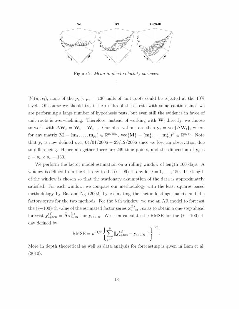
Figure 2: Mean implied volatility surfaces.

.

Wt(ui, vi), none of the pu × pv = 130 nulls of unit roots could be rejected at the 10%

level. Of course we should treat the results of these tests with some caution since we

are performing a large number of hypothesis tests, but even still the evidence in favor of

unit roots is overwhelming. Therefore, instead of working with Wt directly, we choose

to work with ∆Wt = Wt − Wt−1. Our observations are then yt = vec{∆Wt}, where

for any matrix M = (m1, . . . ,mpv) ∈ R

pu×pv , vec{M} = (mT1 , . . . ,mT

pv)T ∈ R

pupv . Note

that yt is now defined over 04/01/2006 − 29/12/2006 since we lose an observation due

to differencing. Hence altogether there are 249 time points, and the dimension of yt is

p = pv × pu = 130.

We perform the factor model estimation on a rolling window of length 100 days. A

window is defined from the i-th day to the (i + 99)-th day for i = 1, · · · , 150. The length

of the window is chosen so that the stationary assumption of the data is approximately

satisfied. For each window, we compare our methodology with the least squares based

methodology by Bai and Ng (2002) by estimating the factor loadings matrix and the

factors series for the two methods. For the i-th window, we use an AR model to forecast

the (i+100)-th value of the estimated factor series x(1)i+100, so as to obtain a one-step ahead

forecast y(1)i+100 = Ax

(1)i+100 for yi+100. We then calculate the RMSE for the (i + 100)-th

day defined by

RMSE = p−1/2

{p∑

j=1

‖y(1)i+100 − yi+100‖

2

}1/2

.

More in depth theoretical as well as data analysis for forecasting is given in Lam et al.

(2010).

18

6.1 Estimation results

In forming the matrix L for each window, we take k0 = 5 in (2.5) , taking advantage

that the autocorrelations are not weak even at higher lags, though similar results (not

reported here) are obtained for smaller k0.

Figure 3: Average of each ordered eigenvalue of L over the 150 windows. Left: Ten

largest. Right: Second to eleventh largest.

Figure 3 displays the average of each ordered eigenvalue over the 150 windows. The

left hand side shows the average of the largest to the average of the tenth largest eigenvalue

of L for Dell, IBM and Microsoft for our method, whereas the right hand side shows the

second to eleventh largest. We obtain similar results for the Bai and Ng (2002) procedure

and thus the corresponding graph is not shown.

From this graphic it is apparent that there is one eigenvalue that is much larger than

the others for all three companies for each window. We have done automatic selection

for the number of factors for each window using the ICp1 criterion in Bai and Ng (2002)

and a one factor model is consistently obtained for each window and for each company.

Hence both methods chose a one factor model over the 150 windows.

Figure 4 displays the cumulative RMSE over the 150 windows for each method. We

choose a benchmark procedure (green line in each plot), where we just treat today’s

value as the one-step ahead forecast. Except for Dell where Bai and Ng (2002) procedure

19

Figure 4: The cumulative RMSE over the 150 windows. Red: Bai and Ng (2002) proce-

dure. Green: Taking forecast y(1)t+1 to be yt. Black: Our methodology.

is doing marginally better, our methodology consistently outperforms the benchmark

procedure and is better than Bai and Ng (2002) for IBM and Microsoft.

7 Proofs

First of all, we show how model (2.2) can be derived from (2.1).

Applying the standard QR decomposition, we may write A = QR, where Q is a p×r

matrix such that QT Q = Ir, R is an r × r upper triangular matrix. Therefore model

(2.1) can be expressed as

yt = Qx′t + ǫt,

where x′t = Rxt. With assumptions (A) to (C), the diagonal entries of R are all asymp-

totic to p1−δ2 . Since r is a constant, using

‖R‖ = max‖u‖=1

‖Ru‖, ‖R‖min = min‖u‖=1

‖Ru‖,

and the fact that R is an r× r upper triangular matrix with all diagonal elements having

the largest order p1−δ2 , we have

‖R‖ ≍ p1−δ2 ≍ ‖R‖min.

Thus, for k = 1, · · · , k0, Σx′(k) = Cov(x′t−k,x

′t) = RΣx(k)RT , with

p1−δ ≍ ‖R‖2min · ‖Σx(k)‖min ≤ ‖Σx′(k)‖min ≤ ‖Σx′(k)‖ ≤ ‖R‖2 · ‖Σx(k)‖ ≍ p1−δ,

20

so that ‖Σx(k)‖ ≍ p1−δ ≍ ‖Σx(k)‖min. We used ‖AB‖min ≥ ‖A‖min · ‖B‖min, which can

be proved by noting

‖AB‖min = minu6=0

uT BTATABu

‖u‖2≥ min

u6=0

(Bu)TATA(Bu)

‖Bu‖2·‖Bu‖2

‖u‖2

≥ minw 6=0

wTATAw

‖w‖2· min

u6=0

‖Bu‖2

‖u‖2= ‖A‖min · ‖B‖min. (7.1)

Finally, using assumption (A) that Σx,ǫ(k) = O(1) elementwise, and that it has rp ≍ p

elements, we have

‖Σx′,ǫ(k)‖ = ‖RΣx,ǫ(k)‖ ≤ ‖R‖ · ‖Σx,ǫ(k)‖F = O(p1−δ2 ) · O(p1/2) = O(p1−δ/2).

Before proving the theorems in section 3, we need to have three lemmas.

Lemma 1 Under the factor model (2.2) which is a reformulation of (2.1), and under

condition (D) in section 2.2, we have for 0 ≤ k ≤ k0,

‖Σx(k) − Σx(k)‖ = OP (p1−δn−lx), ‖Σǫ(k) − Σǫ(k)‖ = OP (pn−lǫ),

‖Σx,ǫ(k) −Σx,ǫ(k)‖ = OP (p1−δ/2n−lxǫ) = ‖Σǫ,x(k) −Σǫ,x(k)‖,

for some constants 0 < lx, lxǫ, lǫ ≤ 1/2. Moreover, ‖xt‖2 = OP (p1−δ) for all real t.

Proof. Using the notations in section 2.2, let xt be the factors in model (2.1), and

x′t be the factors in model (2.2), with the relation that x′

t = Rxt, where R is an upper

triangular matrix with ‖R‖ ≍ p1−δ2 ≍ ‖R‖min (see the start of this section for more details

on R). Then we immediately have ‖x′t‖

2 ≤ ‖R‖2 · ‖xt‖2 = OP (p1−δr) = OP (p1−δ).

Also, the covariance matrix and the sample covariance matrix for {x′t} are respectively

Σx′(k) = RΣx(k)RT , Σx′(k) = RΣx(k)RT ,

where Σx(k) and Σx(k) are respectively the covariance matrix and the sample covariance

matrix for the factors {xt}. Hence

‖Σx′(k) − Σx′(k)‖ ≤ ‖R‖2 · ‖Σx(k) − Σx(k)‖

= O(p1−δ) · OP (n−lx · r)

= OP (p1−δn−lx),

21

which is the rate specified in the lemma. We used the fact that the matrix Σx(k)−Σx(k)

has r2 elements, with elementwise rate of convergence being O(n−lx) as in assumption

(D). Other rates can be derived similarly. �

The following is Theorem 8.1.10 in Golub and Van Loan (1996), which is stated ex-

plicitly since most of our main theorems are based on this. See Johnstone and Arthur

(2009) also.

Lemma 2 Suppose A and A + E are n × n symmetric matrices and that

Q = [Q1 Q2] (Q1 is n × r, Q2 is n × (n − r))

is an orthogonal matrix such that span(Q1) is an invariant subspace for A (i.e., span(Q1) ⊂

span(A)). Partition the matrices QTAQ and QTEQ as follows:

QTAQ =

(D1 0

0 D2

)QTEQ =

(E11 ET

21

E21 E22

).

If sep(D1,D2) := minλ∈λ(D1), µ∈λ(D2) |λ−µ| > 0, where λ(M) denotes the set of eigenval-

ues of the matrix M , and

‖E‖ ≤sep(D1,D2)

5,

then there exists a matrix P ∈ R(n−r)×r with

‖P‖ ≤4

sep(D1,D2)‖E21‖

such that the columns of Q1 = (Q1 +Q2P)(I+PTP)−1/2 define an orthonormal basis for

a subspace that is invariant for A + E.

Proof of Theorem 1. Under model (2.2), the assumption that ‖Σx,ǫ(k)‖ = o(‖Σx(k)‖),

and the definition of L and Dx in section 2.3 such that LA = ADx, Dx has non-zero

eigenvalues of order p2−2δ, contributed by the term Σx(k)Σx(k)T . If B is an orthogonal

complement of A, then LB = 0, and(

AT

BT

)L(A B) =

(Dx 0

0 0

), (7.2)

with sep(Dx, 0) = λmin(Dx) ≍ p2−2δ (see Lemma 2 for the definition of the function sep).

Define EL = L − L, where L is defined in (2.5). Then it is easy to see that

‖EL‖ ≤

k0∑

k=1

{‖Σy(k) − Σy(k)‖2 + 2‖Σy(k)‖ · ‖Σy(k) − Σy(k)‖

}. (7.3)

22

Suppose we can show further that

‖EL‖ = OP (p2−2δn−lx + p2−3δ/2n−lxǫ + p2−δn−lǫ) = OP (p2−2δhn), (7.4)

then since hn = o(1), we have from (7.2) that

‖EL‖ = OP (p2−2δhn) ≤ sep(Dx, 0)/5

for sufficiently large n. Hence we can apply Lemma 2 to conclude that there exists a

matrix P ∈ R(p−r)×r such that

‖P‖ ≤4

sep(Dx, 0)‖(EL)21‖ ≤

4

sep(Dx, 0)‖EL‖ = OP (hn),

and A = (A + BP)(I + PTP)−1/2 is an estimator for A. Then we have

‖A −A‖ = ‖(A(I− (I + PTP)1/2) + BP)(I + PTP)−1/2‖

≤ ‖I− (I + PTP)1/2‖ + ‖P‖

≤ 2‖P‖ = OP (hn).

Hence it remains to show (7.4). To this end, consider for k ≥ 1,

‖Σy(k)‖ = ‖AΣx(k)AT + AΣx,ǫ(k)‖ ≤ ‖Σx(k)‖ + ‖Σx,ǫ(k)‖ = O(p1−δ) (7.5)

by assumptions in model (2.2) and ‖Σx,ǫ(k)‖ = o(‖Σx(k)‖). Finally, noting ‖A‖ = 1,

‖Σy(k) −Σy(k)‖ ≤‖Σx(k) − Σx(k)‖ + 2‖Σx,ǫ(k) − Σx,ǫ(k)‖

+ ‖Σǫ(k) − Σǫ(k)‖

=OP (p1−δn−lx + p1−δ/2n−lxǫ + pn−lǫ)

(7.6)

by Lemma 1. With (7.5) and (7.6), we can conclude from (7.3) that

‖EL‖ = OP (‖Σy(k)‖ · ‖Σy(k) −Σy(k)‖),

which is exactly the order specified in (7.4). �

Proof of Theorem 2. For the sample covariance matrix Σy, note that (7.6) is

applicable to the case when k = 0, so that

‖Σy − Σy‖ = OP (p1−δn−lx + p1−δ/2n−lxǫ + pn−lǫ) = OP (p1−δhn).

23

For Σy, we have

‖Σy − Σy‖ ≤ ‖AΣxAT −AΣxA

T‖ + ‖Σǫ −Σǫ‖

= OP (‖A −A‖ · ‖Σx‖ + ‖Σx − Σx‖ + ‖Σǫ − Σǫ‖).(7.7)

We first consider ‖Σǫ − Σǫ‖ = max1≤j≤p |σ2j − σ2

j | ≤ I1 + I2 + I3, where

I1 = n−1s−1‖∆j(Ip − AAT )AX‖2F ,

I2 = |n−1s−1‖∆j(Ip − AAT )E‖2F − σ2

j |,

I3 = 2n−1s−1‖∆j(Ip − AAT )AX‖F · ‖∆j(Ip − AAT )E‖F ,

with X = (x1 · · ·xn), E = (ǫ1 · · ·ǫn). We have

I1 ≤ n−1s−1‖∆j(Ip − AAT )(A − A)X‖2F

≤ n−1s−1‖∆j‖2 · ‖Ip − AAT‖2 · ‖A− A‖2 · ‖X‖2

F

= OP (p1−δs−1h2n), (7.8)

where we used Theorem 1 for the rate ‖A−A‖2 = OP (h2n), and Lemma 1 to get ‖X‖2

F =

OP (p1−δn). Also we used ‖∆j‖ = 1 and ‖Ip − AAT‖ ≤ 2. For I2, consider

I2 ≤ |n−1s−1‖∆jE‖2F − σ2

j | + n−1s−1‖∆jAATE‖2F

= OP (n−lǫ) + OP (n−1s−1(‖∆jAATE‖2F + ‖∆jA(A− A)TE‖2

F ))

= OP (n−lǫ) + OP (n−1s−1(‖ATE‖2F + ‖(A− A)TE‖2

F ))

= OP (n−lǫ) + OP (n−1s−1(‖ATE‖2F )), (7.9)

where we used assumption (D) in arriving at |n−1s−1‖∆jE‖2F − σ2

j | = oP (n−lǫ), and that

‖(A−A)TE‖F ≤ ‖ATE‖F for sufficiently large n since ‖A−A‖ = oP (1). Consider aTi ǫj

which is the (i, j)-th element of ATE. We have

E(aTi ǫj) = 0, Var(aT

i ǫj) = aTi Σǫai ≤ max

1≤j≤pσ2

j = O(1)

since the σ2j ’s are uniformly bounded away from infinity by assumption (M1). Hence each

element in ATE is OP (1), which implies that

n−1s−1‖ATE‖2F = OP (n−1s−1 · rn) = OP (s−1).

Hence from (7.9) we have

I2 = OP (n−lǫ + s−1). (7.10)

24

Assumption (M2) ensures that both I1 and I2 are oP (1) from (7.8) and (7.10) respectively.

From these we can see that I3 = OP (I1/21 ) = OP ((p1−δs−1)1/2hn), which shows that

‖Σǫ −Σǫ‖ = OP ((p1−δs−1)1/2hn). (7.11)

Next we consider ‖Σx − Σx‖ ≤ K1 + K2 + K3 + K4, where

K1 = ‖ATAΣxAT A− Σx‖, K2 = ‖ATAΣx,ǫA‖,

K3 = ‖AT Σǫ,xAT A‖, K4 = ‖AT (Σǫ − Σǫ)A‖,

where Σx = n−1∑n

t=1(xt − x)(xt − x)T . Now

K1 ≤ ‖ATA− Ir‖ · ‖Σx‖ + ‖Σx − Σx‖

= OP (‖ATA − Ir‖ · (‖Σx − Σx‖ + ‖Σx‖) + ‖Σx − Σx‖)

= OP (p1−δhn),

where we used ‖ATA − Ir‖ = ‖(A − A)TA‖ = OP (hn) by Theorem 1, ‖Σx‖ = O(p1−δ)

from assumption in model (2.2), and ‖Σx − Σx‖ = OP (p1−δn−lx) from Lemma 1. Next,

using Lemma 1 and the fact that Σx,ǫ = 0, we have

K2 = OP (K3) = OP (‖Σx,ǫ − Σx,ǫ‖) = OP (p1−δ/2n−lxǫ).

Finally, using Lemma 1 again and (7.11),

K4 = OP (‖Σǫ − Σǫ‖ + ‖Σǫ − Σǫ‖) = OP ((p1−δs−1)1/2hn + pn−lǫ).

Looking at the rates for K1 to K4, and noting assumption (M2) and the definition of hn,

we can easily see that

‖Σx −Σx‖ = OP (p1−δhn). (7.12)

From (7.7), combining (7.11) and (7.12) and noting assumption (M2), the rate for Σy in

the spectral norm is established, and the proof of the theorem completes. �

Proof of Theorem 3. We first show the rate for Σy. We use the standard inequality

‖M−11 − M−1

2 ‖ ≤‖M−1

2 ‖2 · ‖M1 − M2‖

1 − ‖(M1 − M2) · M−12 ‖

, (7.13)

25

with M1 = Σy and M2 = Σy. Under assumption (M1) we have ‖Σǫ‖ ≍ 1 ≍ ‖Σ−1ǫ‖, so

that

‖Σ−1y ‖ = ‖Σ−1

ǫ− Σ−1

ǫA(Σ−1

x + ATΣ−1ǫ

A)−1ATΣ−1ǫ‖

= O(‖Σ−1ǫ‖ + ‖Σ−1

ǫ‖2 · ‖(Σ−1

x + ATΣ−1ǫ

A)−1‖)

= O(1),

where we also used

‖(Σ−1x + ATΣ−1

ǫA)−1‖ ≤ ‖(ATΣ−1

ǫA)−1‖

= λmax{(ATΣ−1

ǫA)−1} = λ−1

min(ATΣ−1

ǫA) = O(1), (7.14)

since the eigenvalues of Σ−1ǫ

are of constant order by assumption (M1), and ‖A‖min = 1

with Ax 6= 0 for any x since A is of full rank with p > r, so that

λmin(ATΣ−1

ǫA) = min

x 6=0

xTATΣ−1ǫ

Ax

‖x‖≥ min

y 6=0

yTΣ−1ǫ

y

‖y‖· min

x 6=0

‖Ax‖

‖x‖

= λmin(Σ−1ǫ

) · ‖A‖min ≍ 1. (7.15)

Then by (7.13) together with Theorem 2 that ‖Σy−Σy‖ = OP (p1−δhn) = oP (1), we have

‖Σ−1

y − Σ−1y ‖ =

O(1)2 · OP (p1−δhn)

1 − oP (1)= OP (p1−δhn),

which is what we need to show.

Now we show the rate for Σ−1

y . Using the Sherman-Morrison-Woodbury formula, we

have ‖Σ−1

y − Σ−1y ‖ ≤

∑6j=1 Kj , where

K1 = ‖Σ−1

ǫ− Σ−1

ǫ‖,

K2 = ‖(Σ−1

ǫ− Σ−1

ǫ)A(Σ

−1

x + AT Σ−1

ǫA)−1AT Σ

−1

ǫ‖,

K3 = ‖Σ−1ǫ

A(Σ−1

x + AT Σ−1

ǫA)−1AT (Σ

−1

ǫ−Σ−1

ǫ)‖,

K4 = ‖Σ−1ǫ

(A −Ax)(Σ−1

x + AT Σ−1

ǫA)−1ATΣ−1

ǫ‖,

K5 = ‖Σ−1ǫ

Ax(Σ−1

x + AT Σ−1

ǫA)−1(A− Ax)

TΣ−1ǫ‖,

K6 = ‖Σ−1ǫ

Ax{(Σ−1

x + AT Σ−1

ǫA)−1 − (Σ−1

x + ATΣ−1ǫ

A)−1}ATΣ−1ǫ‖.

(7.16)

First, we have ‖Σ−1ǫ‖ = O(1) as before by assumption (M1). Next,

K1 = max1≤j≤k

|σ−2j − σ−2

j | =max1≤j≤k |σ

2j − σ2

j |

min1≤j≤k σ2j (σ

2j + OP ((p1−δs−1)1/2hn))

= OP ((p1−δs−1)1/2hn),

26

where we used (7.11) and assumptions (M1) and (M2). From these, we have

‖Σ−1

ǫ‖ = OP (1). (7.17)

Also, like (7.14),

‖(Σx + AT Σ−1

ǫA)−1‖ = OP (1), (7.18)

noting (7.11) and assumption (M1). With these rates and noting that ‖Ax‖ = ‖A‖ = 1

and ‖A− Ax‖ = OP (hn) from Theorem 1, we have from (7.16) that

‖Σ−1

y − Σ−1y ‖ = OP ((p1−δs−1)1/2hn + hn)

+ OP (‖(Σ−1

x + AT Σ−1

ǫA)−1 − (Σ−1

x + ATΣ−1ǫ

A)−1‖),(7.19)

where the last term is contributed from K6. Using (7.14) and (7.18), and the inequality

‖M−11 − M−1

2 ‖ = OP (‖M−11 ‖ · ‖M1 − M2‖ · ‖M

−12 ‖), the rate for this term can be shown

to be OP (L1 + L2), where

L1 = ‖Σ−1

x − Σ−1x ‖, L2 = ‖AT Σ

−1

ǫA− ATΣ−1

ǫA‖.

Consider ‖Σ−1x ‖ ≤ ‖Σ−1

x ‖ = λ−1min(Σx) = O(p−(1−δ)) by assumption in model (2.2). With

this and (7.12), substituting M1 = Σx and M2 = Σx into (7.13), we have

L1 =O(p−(2−2δ)) · OP (p1−δhn)

1 − OP (p1−δhn · p−(1−δ))=

OP (p−(1−δ)hn)

1 − oP (1)= OP (p−(1−δ)hn). (7.20)

For L2, using ‖A‖ = ‖A‖ = 1, ‖A − A‖ = OP (hn) from Theorem 1, the rate for K1

shown before and (7.17), we have

L2 = OP (‖A− A‖ · ‖Σ−1

ǫ‖ + ‖Σ

−1

ǫ− Σ−1

ǫ‖) = OP (hn + (p1−δs−1)1/2hn). (7.21)

Hence, from (7.19), together with (7.20) and (7.21), we have

‖Σ−1

y − Σ−1y ‖ = OP ((1 + (p1−δs−1)1/2)hn),

which completes the proof of the theorem. �

Proof of Theorem 4. The idea of the proof is similar to that for Theorem 1 for the

simple procedure. We want to find the order of the eigenvalues of the matrix L first.

27

From model (4.9), we have for i = 1, 2,

‖Σii(k)‖2 ≍ p2−2δi ≍ ‖Σii(k)‖min,

‖Σ12(k)‖2 ≍ p2−δ1−δ2 ≍ ‖Σ12(k)‖min,

‖Σiǫ(k)‖2 ≍ p2−δi ≍ ‖Σiǫ(k)‖.

(7.22)

We want to find the lower bounds of the order of the r1-th largest eigenvalue, as well as

the smallest non-zero eigenvalue of L. We first note that

Σy(k) = A1Σ11(k)AT1 + A1Σ12(k)AT

2 + A2Σ21(k)AT1

+ A2Σ22(k)AT2 + A1Σ1ǫ(k) + A2Σ2ǫ(k), (7.23)

and hence

L = A1W1AT1 + A2W2A

T2 + cross terms, (7.24)

where W1 (with size r1×r1) and W2 (with size r2×r2) are positive semi-definite matrices

defined by

W1 =

k0∑

k=1

{Σ11(k)Σ11(k)T + Σ12(k)Σ12(k)T + Σ1ǫ(k)Σ1ǫ(k)T

},

W2 =

k0∑

k=1

{Σ21(k)Σ21(k)T + Σ2ǫ(k)Σ2ǫ(k)T + Σ22(k)Σ22(k)T

}.

From W1, by (7.22) and that ‖Σ1ǫ(k)‖ = o(‖Σ11(k)‖), we have the order of the r1

eigenvalues for W1 is all p2−2δ1 . Then the r1-th largest eigenvalue of L is of order p2−2δ1

since the term Σ11(k)Σ11(k)T has the largest order at p2−2δ1 . We write

p2−2δ1 = OP (λr1(L)), (7.25)

where λi(M) represents the i-th largest eigenvalue of the square matrix M .

For the smallest non-zero eigenvalue of W2, since ‖Σ2ǫ(k)‖ = o(‖Σ22(k)‖), it is

contributed either from the term Σ22(k)Σ22(k)T or Σ21(k)Σ21(k)T in W2, and has order

p2−2δ2 if ‖Σ21(k)‖min = o(p2−2δ2), and p2−c in general if ‖Σ21(k)‖min ≍ p2−c, with δ1+δ2 ≤

c ≤ 2δ2. Hence

p2−2δ2 = OP (λr1+r2(L)), if ‖Σ21(k)‖min = o(p2−2δ2),

p2−c = OP (λr1+r2(L)), if ‖Σ21(k)‖min ≍ p2−c, δ1 + δ2 ≤ c < 2δ2.

(7.26)

28

Now we can write L = (A B)Dx(A B)T , where B is the orthogonal complement of

A, and with Dx1 containing the r1 largest eigenvalues of L and Dx2 the next r2 largest,

Dx =

Dx1 0 0

0 Dx2 0

0 0 0

, (7.27)

with p2−2δ1 = OP (λmin(Dx1)) by (7.25), and p2−c = OP (λmin(Dx2)) by (7.26), δ1 + δ2 ≤

c ≤ 2δ2.

Similar to the proof of Theorem 1, we define EL = L− L. Then (7.3) holds, and

‖Σy(k)‖ = OP (p1−δ1), (7.28)

using (7.23) and ‖Σ11(k)‖ = OP (p1−δ1) from (7.22).

Also,

‖Σy(k) − Σy(k)‖ = OP (‖Σ11(k) − Σ11(k)‖ + ‖Σ12(k) −Σ12(k)‖

+ ‖Σ22(k) −Σ22(k)‖ + ‖Σ1ǫ(k) − Σ1ǫ(k)‖

+ ‖Σ2ǫ(k) − Σ2ǫ(k)‖ + ‖Σǫ(k) − Σǫ(k)‖)

= OP (p1−δ1n−l1 + p1−δ2n−l2 + p1−δ1/2−δ2/2n−l12

+ p1−δ1/2n−l1ǫ + p1−δ2/2n−l2ǫ + pn−lǫ) = OP (p1−δ1ω1), (7.29)

where we used condition (D’) in section 4.2 to derive the following rates like those in

Lemma 1 (proofs thus omitted):

‖Σ11(k) − Σ11(k)‖ = OP (p1−δ1n−l1), ‖Σ12(k) − Σ12(k)‖ = OP (p1−δ1/2−δ2/2n−l12),

‖Σ22(k) − Σ22(k)‖ = OP (p1−δ2n−l2), ‖Σ1ǫ(k) − Σ1ǫ(k)‖ = OP (p1−δ1/2n−l1ǫ),

‖Σ2ǫ(k) − Σ2ǫ(k)‖ = OP (p1−δ2/2n−l2ǫ), ‖Σǫ(k) −Σǫ(k)‖ = OP (pn−lǫ).

(7.30)

We form A1 with the first r1 unit eigenvectors corresponding to the r1 largest eigen-

values, i.e. the eigenvalues in Dx1. Now, we have

‖EL‖ = OP (‖Σy(k) − Σy(k)‖ · (‖Σy(k)‖ + ‖Σy(k) −Σy(k)‖)) = OP (p2−2δ1ω1)

= oP (p2−2δ1) = OP (λmin(Dx1)), hence asymptotically,

‖EL‖ ≤1

5sep

(Dx1,

(Dx2 0

0 0

) ),

29

where the second equality is from (7.28) and (7.29), the third is from noting that ω1 =

o(1), and the last is from (7.25). Hence, we can use Lemma 2 and arguments similar to

the proof of Theorem 1 to conclude that

‖A1 −A1‖ = OP

(‖EL‖/sep

(Dx1,

(Dx2 0

0 0

) ))= OP (ω1).

Similarly, depending on the order of ‖Σ21(k)‖min, we have

‖EL‖ = OP (p2−2δ1ω1) ≤1

5sep

(Dx2,

(Dx1 0

0 0

) )≍ p2−c,

since we assumed pc−2δ1ω1 = o(1) for δ1 + δ2 ≤ c ≤ 2δ2. Hence

‖A2 −A2‖ = OP

(‖EL‖/sep

(Dx2,

(Dx1 0

0 0

)))= OP (pc−2δ1ω1) = OP (ω2).

This completes the proof for the simple procedure.

For the two-step procedure, denote y∗t = (Ip − A1A

T1 )yt, and define EL∗ = L∗ − L∗.

Note that

‖EL∗‖ = ‖L∗−L∗‖ ≤

k0∑

k=1

{‖Σy∗(k)−Σy∗(k)‖2+‖Σy∗(k)‖·‖Σy∗(k)−Σy∗(k)‖

}, (7.31)

where

Σy∗(k) = (Ip − A1AT1 )Σy(k)(Ip − A1A

T1 ),

Σy∗(k) = (Ip − A1AT1 )Σy(k)(Ip − A1A

T1 ) = A2Σ22(k)AT

2 + A2Σ2ǫ(k)(Ip − A1AT1 ),

L∗ =

k0∑

k=1

Σy∗(k)Σy∗(k)T , L∗ =

k0∑

k=1

Σy∗(k)Σy∗(k)T ,

with A1 being the estimator from the simple procedure, so that ‖A1 − A1‖ = OP (ω1)

from previous result. We write

L∗ = A2Q2D2QT2 AT

2 , so that L∗A2Q2 = A2Q2D2,

and hence we are estimating A′2 = A2Q2.

The idea of the proof is to find the rates of ‖EL∗‖ and the eigenvalues in D2 and use

the arguments similar to the proof for the simple procedure to get the rate for ‖A′2−A′

2‖.

First, with the assumption that ‖Σ22(k)‖ ≍ p1−δ2 ≍ ‖Σ22(k)‖min and ‖Σ2ǫ(k)‖ =

o(‖Σ22(k)‖), all the eigenvalues in D2 have order p2−2δ2 .

30

We need to find ‖EL∗‖. It is easy to show that

‖A1AT1 A2‖ = ‖A1(A1 − A1)

TA2‖ ≤ ‖A1 −A1‖ = OP (ω1),

‖(Ip − A1AT1 )A1‖ = ‖(A1 − A1) − A1(A1 −A1)

TA1‖ = OP (ω1).(7.32)

Writing H1 = Ip − A1AT1 , we can decompose Σy∗(k) − Σy∗(k) =

∑9l=1 Il, where

I1 = H1A1Σ11(k)AT1 H1, I2 = H1A1Σ12(k)AT

2 H1,

I3 = H1A1Σ1ǫ(k)H1, I4 = H1A2Σ21(k)AT1 H1,

I5 = H1A2Σ22(k)AT2 H1 −A2Σ22(k)AT

2 , I6 = H1A2Σ2ǫ(k)H1 − A2Σ2ǫ(k)H1,

I7 = H1Σǫ1(k)AT1 H1, I8 = H1Σǫ2(k)AT

2 H1, I9 = H1Σǫ(k)H1.

Using (7.30), (7.32) and the assumptions in model (4.9), we can see that

‖I1‖ = OP (‖H1A1‖2 · ‖Σ11(k)‖) = OP (p1−δ1ω2

1),

‖I2‖ = OP (‖H1A1‖ · ‖Σ12(k)‖) = OP (p1−δ1/2−δ2/2ω1) = ‖I4‖,

‖I7‖ = OP (‖I3‖) = OP (‖H1A1‖ · (‖Σ1ǫ(k) −Σ1ǫ(k)‖ + ‖Σ1ǫ(k)‖)) = OP (p1−δ1ω1),

‖I6‖ = OP (‖Σ2ǫ(k) −Σ2ǫ(k)‖ + ‖Σ2ǫ(k)‖ · ‖A1 −A1‖) = OP (p1−δ2/2(n−l2ǫ + p−δ2/2ω1)),

‖I8‖ = OP (‖Σǫ2(k)‖) = OP (p1−δ2/2n−l2ǫ), ‖I9‖ = OP (‖Σǫ‖) = OP (pn−lǫ),

‖I5‖ = OP (‖A1AT1 A2‖ · ‖Σ22(k)‖ + ‖Σ22(k) −Σ22(k)‖) = OP (p1−δ2(ω1 + n−l2)).

Hence, we have

‖Σy∗(k) − Σy∗(k)‖ = OP (p1−δ1ω21 + p1−δ1/2−δ2/2ω1 + p1−δ1ω1

+ p1−δ2/2(n−l2ǫ + p−δ2/2ω1) + pn−lǫ + p1−δ2(ω1 + n−l2))

= OP (p1−δ1ω1). (7.33)

We also have

‖Σy∗(k)‖ = OP (‖Σ22(k)‖ + ‖Σ2ǫ(k)‖) = OP (p1−δ2). (7.34)

Hence, with (7.33) and (7.34), (7.31) becomes

‖EL∗‖ = OP (p2−δ1−δ2ω1). (7.35)

With the order of eigenvalues in D2 being p2−2δ2 and (7.33), we can use Lemma 2 and

the arguments similar to those in the proof of Theorem 1 to get

‖A′2 −A′

2‖ = OP (‖EL∗‖/sep(D2, 0)) = OP (pδ2−δ1ω1),

31

and the proof of the theorem completes. �

Proof of Theorem 5. We have xt = ATyt = ATAxt + (A − A)Tǫt + AT

ǫt. With

A = (A1 A2) and xt = (xT1t xT

2t)T , we have

x1t = AT1 A1x1t + AT

1 A2x2t + (A1 − A1)Tǫt + AT

1 ǫt,

x2t = AT2 A1x1t + AT

2 A2x2t + (A2 − A2)Tǫt + AT

2 ǫt.

We first note that for i = 1, 2, ‖(Ai − Ai)Tǫt‖ = OP (AT

i ǫt) = OP (1) since ‖Ai − Ai‖ =

oP (1) and ATi ǫt are ri OP (1) random variables. Then

‖x1t‖ = ‖x1t‖F ≥ ‖AT1 A1x1t‖F − ‖AT

1 A2x2t‖F + OP (1)

≥ ‖AT1 A1‖min · ‖x1t‖F − ‖AT

1 A2‖ · ‖x2t‖ + OP (1)

≥ ‖A1‖min · ‖A1‖min · ‖x1t‖ − oP (‖x2t‖) + OP (1)

= OP (‖x1t‖) ≍ p1−δ1

2 ,

where ‖M‖F denotes the Frobenius norm of the matrix M , and we used the inequality

‖AB‖F ≥ ‖A‖min · ‖B‖F . Finally, with similar arguments,

‖x2t‖ ≤ ‖x2t‖ + ‖AT2 A2‖ · ‖x1t‖ + OP (1)

= OP (p1−δ2

2 ) + OP (‖A2 − A2‖ · p1−δ1

2 )

= OP (p1−δ2

2 ) + oP (p1−δ1

2 )

= oP (p1−δ1

2 ),

which establishes the claim of the theorem. �

Proof of Theorem 6. We can easily use the decomposition in (7.6) again for model

(4.9) to arrive at

‖Σy − Σy‖ = OP (p1−δ1n−l1 + p1−δ2n−l2 + p1−δ1/2n−l1ǫ + p1−δ2/2n−l2ǫ + pn−lǫ),

= OP (p1−δ1ω1),

where we used assumption (D’), and arguments like those in Lemma 1 to arrive at ‖Σx−

Σx‖ = OP (p1−δ1n−l1 + p1−δ2n−l2), ‖Σx,ǫ − Σx,ǫ‖ = OP (p1−δ1/2n−l1ǫ + p1−δ2/2n−l2ǫ) and

‖Σǫ − Σǫ‖ = OP (pn−lǫ).

Now consider ‖Σy−Σy‖, which can be decomposed like that in (7.7). Hence we need

to consider ‖Σǫ − Σǫ‖ = max1≤j≤p |σ2j − σ2

j | ≤ I1 + I2 + I3, where

I1 = OP (p1−δ1s−1‖A− A‖2),

32

which used decomposition in (7.8), and ‖X‖2F = OP (p1−δ1nr1 + p1−δ2nr2) = OP (p1−δ1n);

I2 = OP (n−lǫ + s−1),

where derivation is similar to that in (7.9) and thereafter. Also, I3 = OP (I1/21 ) =

OP ((p1−δ1s−1)1/2‖A − A‖). Thus, with assumption (M2)’, we see that

‖Σǫ − Σǫ‖ = OP ((p1−δ1s−1)1/2‖A −A‖). (7.36)

For ‖Σx − Σx‖, we use the decomposition like that in the proof of Theorem 2, and

noting that ‖Σx‖ = O(p1−δ1 + p1−δ2) = O(p1−δ1), to arrive at

‖Σx − Σx‖ = OP (p1−δ1‖A −A‖). (7.37)

Hence noting assumption (M2)’ again and combining (7.36) and (7.37), we see that

‖Σy − Σy‖ = OP (p1−δ1‖A −A‖),

which completes the proof of the theorem. �

Proof of Theorem 7. We omit the rate for Σy since it involves standard treatments

like that in Theorem 3.

Note that (7.19) becomes

‖Σ−1

y − Σ−1y ‖ = OP ((1 + (p1−δ1s−1)1/2)‖A −A‖) + OP (L1 + L2),

with L1 and L2 defined similar to those in the proof of Theorem 3. Similar to (7.20) and

(7.21), we have respectively

L1 = OP (p−(1−δ2)‖A −A‖), L2 = OP ((1 + (p1−δ1s−1)1/2)‖A− A‖),

which shows that ‖Σ−1

y − Σ−1y ‖ = OP ((1 + (p1−δ1s−1)1/2)‖A − A‖). This completes the

proof of the theorem. �

References

Anderson, T. (1963). The use of factor analysis in the statistical analysis of multiple time

series. Psychometrika 28, 1–25.

33

Bai, J. (2003, January). Inferential theory for factor models of large dimensions. Econo-

metrica 71 (1), 135–171.

Bai, J. and S. Ng (2002). Determining the number of factors in approximate factor

models. Econometrica 70 (1), 191–221.

Bai, J. and S. Ng (2007, January). Determining the number of primitive shocks in factor

models. Journal of Business & Economic Statistics 25, 52–60.

Bathia, N., Q. Yao, and F. Zieglemann (2009). Identifying the finite dimensionality of

curve time series. Manuscript.

Brillinger, D. (1981). Time Series Data Analysis and Theory (Extended ed.). San Fran-

cisco: Holden-Day.

Chamberlain, G. and M. Rothschild (1983). Arbitrage, factor structure, and mean-

variance analysis on large asset markets. Econometrica 51, 1281–1304.

Chudik, A., M. H. Pesaran, and E. Tosetti (2009, June). Weak and strong cross section

dependence and estimation of large panels. Manuscript.

Cont, R. and J. da Fonseca (1988). Dynamics of implied volatility surfaces. Quantitative

Finance 2, 45–60.

Fan, J., Y. Fan, and J. Lv (2008, November). High dimensional covariance matrix esti-

mation using a factor model. Journal of Econometrics 147 (1), 186–197.

Fengler, M., W. Hardle, and E. Mammen (2007). A dynamic semiparametric factor model

for implied volatility string dynamics. Journal of Econometrics 5, 189–218.

Forni, M., M. Hallin, M. Lippi, and L. Reichlin (2002, June). The generalized dynamic

factor model: One-sided estimation and forecasting. CEPR Discussion Papers 3432,

C.E.P.R. Discussion Papers.

Golub, G. and C. Van Loan (1996). Matrix Computations (3rd ed.). Johns Hopkins

University Press.

Hallin, M. and R. Liska (2007, June). Determining the number of factors in the general

dynamic factor model. J. Amer. Statist. Assoc. 102, 603–617.

34

Johnstone, I. and Y. Arthur (2009). On consistency and sparsity for principal components

analysis in high dimensions. J. Amer. Statist. Assoc. 104 (486), 682–693.

Lam, C., Q. Yao, and N. Bathia (2010). Forecasting for time series data through factor

modeling. Manuscript.

Pan, J. and Q. Yao (2008). Modelling multiple time series via common factors.

Biometrika 95 (2), 365–379.

Park, B., E. Mammen, W. Hardle, and S. Borak (2009). Modelling dynamic semipara-

metric factor models. J. Amer. Statist. Assoc..

Pena, D. and G. Box (1987). Identifying a simplifying structure in time series.

J. Amer. Statist. Assoc. 82, 836–843.

Pena, D. and P. Poncela (2006). Nonstationay dynamic factor analysis. Journal of

Statistical Planning and Inference 136, 1237–1257.

Priestley, M.B., R. T. and J. Tong (1974). Applications of principal component analysis

and factor analysis in the identification of multivariable systems. IEEE Trans. Automat.

Control 19, 703–704.

35