estimation of level and change for unemployment using

Survey Methodology

Catalogue no. 12-001-X ISSN 1492-0921

by Harm Jan Boonstra and Jan A. van den Brakel

Estimation of level and change for unemployment using structural time series models

Release date: December 17, 2019

Published by authority of the Minister responsible for Statistics Canada

© Her Majesty the Queen in Right of Canada as represented by the Minister of Industry, 2019

All rights reserved. Use of this publication is governed by the Statistics Canada Open Licence Agreement.

An HTML version is also available.

Cette publication est aussi disponible en français.

How to obtain more informationFor information about this product or the wide range of services and data available from Statistics Canada, visit our website, www.statcan.gc.ca. You can also contact us by Email at [email protected] Telephone, from Monday to Friday, 8:30 a.m. to 4:30 p.m., at the following numbers:

• Statistical Information Service 1-800-263-1136 • National telecommunications device for the hearing impaired 1-800-363-7629 • Fax line 1-514-283-9350

Depository Services Program

• Inquiries line 1-800-635-7943 • Fax line 1-800-565-7757

Standards of service to the publicStatistics Canada is committed to serving its clients in a prompt, reliable and courteous manner. To this end, Statistics Canada has developed standards of service that its employees observe. To obtain a copy of these service standards, please contact Statistics Canada toll-free at 1-800-263-1136. The service standards are also published on www.statcan.gc.ca under “Contact us” > “Standards of service to the public.”

Note of appreciationCanada owes the success of its statistical system to a long-standing partnership between Statistics Canada, the citizens of Canada, its businesses, governments and other institutions. Accurate and timely statistical information could not be produced without their continued co-operation and goodwill.

https://www.statcan.gc.ca/eng/reference/licence

https://www150.statcan.gc.ca/n1/pub/12-001-x/2019003/article/00005-eng.htm

https://www.statcan.gc.ca

mailto:STATCAN.infostats-infostats.STATCAN%40canada.ca?subject=

https://www.statcan.gc.ca

https://www.statcan.gc.ca/eng/about/service/standards

Survey Methodology, December 2019 395 Vol. 45, No. 3, pp. 395-425 Statistics Canada, Catalogue No. 12-001-X

1. Harm Jan Boonstra, Statistics Netherlands, Department of Statistical Methods. E-mail: [email protected]; Jan A. van den Brakel, Statistics

Netherlands, Department of Statistical Methods and Maastricht University, Department of Quantitative Economics.

Estimation of level and change for unemployment using structural time series models

Harm Jan Boonstra and Jan A. van den Brakel1

Abstract

Monthly estimates of provincial unemployment based on the Dutch Labour Force Survey (LFS) are obtained using time series models. The models account for rotation group bias and serial correlation due to the rotating panel design of the LFS. This paper compares two approaches of estimating structural time series models (STM). In the first approach STMs are expressed as state space models, fitted using a Kalman filter and smoother in a frequentist framework. As an alternative, these STMs are expressed as time series multilevel models in an hierarchical Bayesian framework, and estimated using a Gibbs sampler. Monthly unemployment estimates and standard errors based on these models are compared for the twelve provinces of the Netherlands. Pros and cons of the multilevel approach and state space approach are discussed.

Multivariate STMs are appropriate to borrow strength over time and space. Modeling the full correlation matrix between time series components rapidly increases the numbers of hyperparameters to be estimated. Modeling common factors is one possibility to obtain more parsimonious models that still account for cross-sectional correlation. In this paper an even more parsimonious approach is proposed, where domains share one overall trend, and have their own independent trends for the domain-specific deviations from this overall trend. The time series modeling approach is particularly appropriate to estimate month-to-month change of unemployment.

Key Words: Small area estimation; Structural time series models; Time series multilevel models; Unemployment

estimation.

1 Introduction

Statistics Netherlands uses data from the Dutch Labour Force Survey (LFS) to estimate labour status at

various aggregation levels. National estimates are produced monthly, provincial estimates quarterly, and

municipal estimates annually. Traditionally monthly publications about the labour force were based on

rolling quarterly figures compiled by means of direct generalized regression estimation (GREG), see e.g.,

Särndal, Swensson and Wretman (1992). The continuous nature of the LFS allows to borrow strength not

only from other areas, but also over time. A structural time series model (STM) to estimate national monthly

labour status for 6 gender by age classes is in use since 2010 (van den Brakel and Krieg, 2009, 2015).

Until now, provincial estimates are produced quarterly using the GREG. In order to produce figures on

a monthly basis, a model-based estimation strategy is necessary to overcome the problem of too small

monthly provincial sample sizes. In this paper a model is proposed that combines a time series modeling

approach to borrow strength over time with cross-sectional small area models to borrow strength over space

with the purpose to produce reliable monthly estimates of provincial unemployment. As a consequence of

the LFS panel design, the monthly GREG estimates are autocorrelated and estimates based on follow-up

waves are biased relative to the first wave estimates. The latter phenomena is often referred to as rotation

group bias (Bailar, 1975). Both features need to be accounted for in the model (Pfeffermann, 1991). Previous

accounts of regional small area estimation of unemployment, where strength is borrowed over both time

396 Boonstra and van den Brakel: Estimation of level and change for unemployment using structural time series models

Statistics Canada, Catalogue No. 12-001-X

and space, include Rao and Yu (1994); Datta, Lahiri, Maiti and Lu (1999); You, Rao and Gambino (2003);

You (2008); Pfeffermann and Burck (1990); Pfeffermann and Tiller (2006); van den Brakel and Krieg

(2016), see also Rao and Molina (2015), Section 4.4 for an overview.

In this paper, multivariate STMs for provincial monthly labour force data are developed as a form of

small area estimation to borrow strength over time and space, to account for rotation group bias and serial

correlation induced by the rotating panel design. In a STM, an observed series is decomposed in several

unobserved components like a trend, a seasonal component, regression components, other cyclic

components and a white noise term for remaining unexplained variation. These components are based on

stochastic models, to allow them to vary over time. The classical way to fit STMs is to express them as a

state space model and apply a Kalman filter and smoother to obtain optimal estimates for state variables and

signals. The unknown hyperparameters of the models for the state variables are estimated by means of

maximum likelihood (ML) (Harvey, Chapter 3). Alternatively, state space models can be fitted in a Bayesian

framework using a particle filter (Andrieu, Poucet and Holenstein (2010); Durbin and Koopman (2012),

Chapter 9). STMs can also be expressed as time series multilevel models and can be seen as an extension

of the classical Fay-Herriot model (Fay and Herriot, 1979). Connections between structural time series

models and multilevel models have been explored before from several points of view in Knorr-Held and

Rue (2002); Chan and Jeliazkov (2009); McCausland, Miller and Pelletier (2011); Ruiz-Cárdenas, Krainski

and Rue (2012); Piepho and Ogutu (2014); Bollineni-Balabay, van den Brakel, Palm and Boonstra (2016).

In these papers the equivalence between state space model components and multilevel components is made

more explicit. Multilevel models can both be fitted in a frequentist and hierarchical Bayesian framework,

see Rao and Molina (2015), Section 8.3 and 10.9, respectively.

This paper contributes to the small area estimation literature by comparing differences between STMs

for rotating panel designs that are expressed as state space models and as time series multilevel models.

State space models are fitted using a Kalman filter and smoother in a frequentist framework where

hyperparameters are estimated with ML. In this case models are compared using AIC and BIC. Time series

multilevel models are fitted in an hierarchical Bayesian framework, using a Gibbs sampler. Models with

different combinations of fixed and random effects are compared based on the Deviance Information

Criterion (DIC). The estimates based on multilevel and state space models and their standard errors are

compared graphically and contrasted with the initial survey regression estimates. Modeling cross-sectional

correlation in multivariate time series models rapidly increases the number of hyperparameters to be

estimated. One way to obtain more parsimonious models is to use common factor models. In this paper an

alternative approach to model correlations between time series components indirectly is proposed, based on

a global common trend and local trends for the domain-specific deviations.

The paper is structured as follows. In Section 2 the LFS data used in this study are described. Section 3

describes how the survey regression estimator (Battese, Harter and Fuller, 1988) is used to compute initial

estimates. These initial estimates are the input for the STM models, which are discussed in Section 4. In

Section 5 the results based on several state space and multilevel models are compared, including estimates

Survey Methodology, December 2019 397


for period-to-period change for monthly data. Section 6 contains a discussion of the results as well as some

ideas on further work. Throughout the paper we refer to the technical report by Boonstra and van den Brakel

(2016) for additional details and results.

2 The Dutch Labour Force Survey

The Dutch LFS is a household survey conducted according to a rotating panel design in which the

respondents are interviewed five times at quarterly intervals. Each month a stratified two-stage sample of

addresses is selected. All households residing on an address are included in the sample. In this study 72

months of LFS data from 2003 to 2008 are used. During this period the sample design was self-weighted.

The first wave of the panel consists of data collected by means of computer assisted personal interviewing

(CAPI), whereas the four follow-up waves contain data collected by means of computer assisted telephone

interviewing (CATI).

The Netherlands is divided into twelve provinces which serve as the domains for which monthly

unemployment figures are to be estimated. Monthly national sample sizes vary between 5 and 7 thousand

persons in the first wave and between 3 and 5 thousand in the fifth wave. Provincial sample sizes are diverse,

ranging from 31 to 1,949 persons for single wave monthly samples.

LFS data are available at the level of units, i.e., persons. A wealth of auxiliary data from several

registrations is also available at the unit level. Among these auxiliary variables is registered unemployment,

a strong predictor for the unemployment variable of interest. These predictors are used to compute initial

estimates, which are input to the time series models.

The target variable considered in this study is the fraction of unemployed in a domain, and is defined as

= ,it ijt itj iY y N

with ijty equal to one if person j from province i in period t is unemployed and

zero otherwise and itN the population size in province i and period .t

3 Initial estimates

Let ˆitpY denote the initial estimate for itY based on data from wave .p The initial estimates used as input

for the time series small area models are survey regression estimates (Woodruff, 1966; Battese et al., 1988;

Särndal et al., 1992)

ˆ ˆ= ,itp itp tp it itpY y X x (3.1)

where ,itpy itpx denote sample means, itX is the vector of population means of the covariates ,x and ˆtp

are estimated regression coefficients. The coefficients are estimated separately for each period and each

wave, but they are based on the national samples combining data from all areas. The survey regression

estimator is an approximately design-unbiased estimator for the population parameters that, like the GREG

estimator, uses auxiliary information to reduce nonresponse bias. See Boonstra and van den Brakel (2016)

for more details on the model selected to compute the survey regression estimates. Even though the



regression coefficient estimates in (3.1) are not area-specific, the survey regression estimator is a direct

domain estimator in the sense that it is primarily based on the data obtained in that particular domain and

month, and therefore it has uncacceptably large standard errors due to the small monthly domain sample

sizes.

The initial estimates for the different waves give rise to systematic differences in unemployment

estimates, generally termed rotation group bias (RGB) (Bailar, 1975). The initial estimates for

unemployement for waves 2 to 5 are systematically smaller compared to the first wave. This RGB has many

possible causes, including selection, mode and panel effects (van den Brakel and Krieg, 2009). See Boonstra

and van den Brakel (2016) for details and graphical illustrations.

The time series models also require variance estimates corresponding to the initial estimates. We use the

following cross-sectionally smoothed estimates of the design variances of the survey regression estimates,

2 2

=1

1 1ˆ ˆ ˆ= 1 ,Am

itp itp itp tp itpiitp tp A

v Y n nn n m

with

2 2

=1

1ˆ ˆ= .

1

itpn

itp ijtpjitp

en

(3.2)

Here Am denotes the number of areas, itpn is the number of respondents in area ,i period t and wave ,p

=1= ,Am

tp itpin n and îjtpe are residuals of the survey regression estimator. The within-area variances 2ˆ itp

are pooled over the domains to obtain more stable variance approximations. The use of (3.2) can be further

motivated as follows. Recall that the sample design is self-weighted. Calculating within-area variances 2ˆ itp

therefore approximately accounts for the stratification, which is a slightly more detailed regional variable

than province. The variance approximation also accounts for calibration and nonresponse correction, since

the within-area variances are calculated over the residuals of the survey regression estimator. The variance

approximation does not explicitly account for the clustering of persons within households. However, the

intra-cluster correlation for unemployment is small. In addition, registered unemployment is used as a

covariate in the survey regression estimator. Since this covariate explains a large part of the variation of

unemployment, the intra-cluster correlation between the residuals is further reduced.

The panel design induces several non-zero correlations among initial estimates for the same province

and different time periods and waves. These correlations are due to partial overlap of the sets of sample

units on which the estimates are based. Such correlations exist between estimates for the same province in

months 1 2,t t and based on waves 1 2,p p whenever 2 1 2 1= 3 12.t t p p The covariances between

1 1

ît pY and

2 2

ît pY are estimated as (see e.g., Kish (1965))

1 1 2 2

1 1 2 2 1 1 2 2 1 1 2 2

1 1 2 2

ˆ ˆ ˆ ˆˆ, = ,it p t pit p it p t p t p it p it p

it p it p

nv Y Y v Y v Y

n n (3.3)

with

1 1 2 2

1 1 2 2 1 1 2 2

1 1 2 2=1 =1

1ˆ ˆ ˆ= ,

it p t pAnm

t p t p ijt p ijt pi jt p t p A

e en m



where 1 1 2 2it p t pn is the number of units in the overlap, i.e., the number of observations on the same units in

area i between period and wave combinations 1 1,t p and 2 2, ,t p and 1 1 2 2 1 1 2 2=1

= .Am

t p t p it p t pin n The

estimated (auto)correlation coefficient 1 1 2 2

ˆ t p t p is computed as the correlation between the residuals of the

linear regression models underlying the survey regression estimators at 1 1,t p and 2 2, ,t p based on the

overlap of both samples over all areas. This way they are pooled over areas in the same way as are the

variances 2ˆ .tp Together, (3.2) and (3.3) estimate (an approximation of) the design-based covariance matrix

for the initial survey regression estimates. See Boonstra and van den Brakel (2016) for more details.

Time series model estimates for monthly provincial unemployment figures will be compared with direct

estimates. The procedure for calculating monthly direct estimates is based on the approach that was used

before 2010 to calculate official rolling quarterly figures for the labour force. Let .ˆ

itY denote the monthly

direct estimate for provinces, which is calculated as the weighted mean over the five panel survey regression

estimates where the weights are based on the variance estimates. To correct for RGB, these direct estimates

are multiplied by a ratio, say ,itf where the numerator is the mean of the survey regression estimates (3.1)

for the first wave over the last three years and the denominator is the mean of monthly direct estimates .ˆ

itY

also over the last three years, i.e., . .ˆ= .it it itY f Y See Boonstra and van den Brakel (2016) for details on

calculating .ˆ

itY and .itY including a variance approximation.

4 Time series small area estimation

The initial monthly domain estimates for the separate waves, accompanied by variance and covariance

estimates, are the input for the time series models. In the next step STM models are applied to smooth the

initial estimates and correct for RGB. The estimated models are used to make predictions for provincial

unemployment fractions, provincial unemployment trends, and month-to-month changes in the trends. In

Subsection 4.1 the STMs are defined and subsequently expressed as state space models fitted in a frequentist

framework. Subsection 4.2 explains how these STMs can be expressed as time series multilevel models

fitted in an hierarchical Bayesian framework.

4.1 State space model

This section develops a structural time series model for the monthly data at provincial level for twelve

provinces simultaneously to take advantage of temporal and cross-sectional sample information. Let

1 5ˆ ˆ ˆ= , ,

t

it it itY Y Y denote the five-dimensional vector containing the survey regression estimates ˆitpY

defined by (3.1) in period t and domain .i This vector can be modeled with the folowing structural time

series model (Pfeffermann, 1991; van den Brakel and Krieg, 2009, 2015):

5ˆ = ,it it it itY e (4.1)

where 5 = 1, 1, 1, 1, 1 ,t it a scalar denoting the true population parameter for period t in domain ,i

it a five-dimensional vector that models the RGB and ite a five-dimensional vector with sampling errors.

The population parameter it in (4.1) is modeled as



= ,it it it itL S (4.2)

where itL denotes a stochastic trend model to capture low frequency variation (trend plus business cycle),

itS a stochastic seasonal component to model monthly fluctuations and it a white noise for the unexplained

variation in .it For the stochastic trend component, the so-called smooth trend model is used, which is

defined by the following set of equations:

ind 21 1 1 , ,= , = , 0, .it it it it it R it R it RiL L R R R N (4.3)

For the stochastic seasonal component the trigonometric form is used, see Boonstra and van den Brakel

(2016) for details. The white noise in (4.2) is defined as ind 20, .iit N

The RGB between the series of the survey regression estimates, is modeled in (4.1) with

1 2 3 4 5= , , , , .tit it it it it it The model is identified by taking 1 = 0.it This implies that the relative

bias in the follow-up waves with respect to the first wave is estimated and it assumes that the survey

regression estimates of the first wave are the most reliable approximations for ,it see van den Brakel and

Krieg (2009) for a motivation. The remaining components model the systematic difference between wave

p with respect to the first wave and are modeled as random walks to allow for time dependent patterns in

the RGB,

ind 21; , ,= , 0, , = 2, 3, 4, 5.

iitp it p itp itp p N (4.4)

Finally, a time series model for the survey errors is developed. Let 1 2 3 4 5= , , , , tit it it it it ite e e e e e denote

the five-dimensional vector containing the survey errors of the five waves. The variance estimates of the

survey regression estimates are used as prior information in the time series model to account for

heteroscedasticity due to varying sample sizes over time using the following survey error model:

ˆ= ,itp itp itpe v Y e (4.5)

and ˆitpv Y defined by (3.2). Since the first wave is observed for the first time there is no autocorrelation

with samples observed in the past. To model the autocorrelation between survey errors of the follow-up

waves, appropriate AR models for ,itpe are derived by applying the Yule-Walker equations to the correlation

coefficients

1 1 2 2

1 1 2 2

1 1 2 2

ˆ ,it p t p

t p t p

it p it p

n

n n (4.6)

which are derived from the micro data as described in Section 3. Based on this analysis an AR(1) model is

assumed for wave 2 through 5 where the autocorrelation coefficients depend on wave and month. These

considerations result in the following model for the survey errors:

1

ind 21 1 1

ind 21 3 1

, 0, ,

, 0, , = 2, , 5,

i

ip

it it it

itp itp itpit p p i t p

e

e e p

N

N

(4.7)



with 1it p p the time-dependent partial autocorrelation coefficients between wave p and 1p derived

from (4.6). As a result, 1

21 1

ˆVar = ,iit ite v Y and 2 2

1ˆVar = 1

ipitp itp it p pe v Y for =p

2, , 5. The variances 2ip are scaling parameters with values close to one for the first wave and close to

211=1

1T

it p pT t for the other waves, where T denotes the length of the observed series.

Model (4.1) uses sample information observed in preceding periods within each domain to improve the

precision of the survey regression estimator and accounts for RGB and serial correlation induced by the

rotating panel design. To take advantage of sample information across domains, model (4.1) for the separate

domains can be combined in one multivariate model:

1 5 1 1 1

5

ˆ

= ,

ˆA A A

A

t t t t

m t m t m tm t

Y e

eY

(4.8)

where Am denotes the number of domains, which is equal to twelve in this application. This multivariate

setting allows to use sample information across domains by modeling the correlation between the

disturbance terms of the different structural time series components (trend, seasonal, RGB) or by defining

the hyperparameters or the state variables of these components equal over the domains. In this paper models

with cross-sectional correlation between the slope disturbance terms of the trend (4.3) are considered, i.e.,

2

,,

if = and =

Cov , = if and = .

0 if

Ri

R itR i t Rii

i i t t

i i t t

t t

(4.9)

The most parsimonious covariance structure is a diagonal matrix where all the domains share the same

variance component, i.e., 2 2=Ri R for all i and = 0Rii

for all i and .i These are so-called seemingly

unrelated structural time series models and are a synthetic approach to use sample information across

domains. A slightly more complex and realistic covariance structure is a diagonal matrix where each domain

has a separate variance component, i.e., = 0Rii

for all i and .i In this case the model only borrows

strength over time and does not take advantage of cross-sectional information. The most complex covariance

structure allows for a full covariance matrix. Strong correlation between the slope disturbances across the

domains can result in cointegrated trends. This implies that < Aq m common trends are required to model

the dynamics of the trends for the Am domains and allows the specification of so-called common trend

models (Koopman, Harvey, Doornik and Shephard, 1999; Krieg and van den Brakel, 2012). Initial STM

analyses showed that the seasonal and RGB component turned out to be time independent. It is therefore

not sensible to model correlations between seasonal and RGB disturbance terms. Since the hyperparameters

of the white noise population domain parameters tend to zero, it turned out to be better to remove this

component completely from the model implying that modeling correlations between population noise is not

considered. Correlations between survey errors for different domains is also not considered, since the

domains are geographical regions from which samples are drawn independently.



As an alternative to a model with a full covariance matrix for the slope disturbances, a trend model is

considered that has one common smooth trend model for all provinces plus 1Am trend components that

describe the deviation of each domain from this overall trend. In this case (4.2) is given by

1 1 1

*

= ,

= , = 2, , .

t t t t

it t it it it A

L S

L L S i m

(4.10)

Here tL is the overal smooth trend component, defined by (4.3), and *itL the deviation from the overall

trend for the separate domains, defined as local levels

ind* * 21 , ,= , 0, ,it it L it L it LiL L N (4.11)

or as smooth trends as in (4.3). These trend models implicitly allow for (positive) correlations between the

trends of the different domains.

The parameters to be estimated with the time series modeling approach are the trend and the signal. The

latter is defined as the trend plus the seasonal component. The time series approach is particularly suitable

for estimating month-to-month changes. Seasonal patterns hamper a straightforward interpretation of

month-to-month changes of direct estimates and smoothed signals. Therefore month-to-month changes are

calculated for the trends only. Due to the strong positive correlation between the levels of consecutive

periods, the standard errors of month-to-month changes in the level of the trends are much smaller than

those of e.g., month-to-month changes of the direct estimates. The month-to-month change of the trend is

defined as 11 =it it itL L for models with separate trends for the domains or 1 =it tL * *

1 1t it itL L L for models with an overall trend and 1Am trends for the deviation from the overall trend

for the separate domains. This modeling approach is also useful to estimate year-to-year developments for

trend defined as 1212 =it it itL L or * *12 1212 = .it t t it itL L L L Year-to-year differences are

also sensible for signals, since the main part of the seasonal component cancels out. These developments

are defined equivalently to the year-to-year developments of the trend.

The aforementioned structural time series models are analyzed by putting them in the so-called state

space form. Subsequently the Kalman filter is used to fit the models, where the unknown hyperparameters

are replaced by their ML estimates. The analysis is conducted with software developed in OxMetrics in

combination with the subroutines of SsfPack 3.0, (Doornik, 2009; Koopman, Shephard and Doornik, 1999,

2008). ML estimates for the hyperparameters are obtained using the numerical optimization procedure

maxBFGS in OxMetrics. More details about the state space representation, initialization of the Kalman filter

and software used to fit these models is included in Boonstra and van den Brakel (2016).

4.2 Time series multilevel model

For the description of the multilevel time series representation of the STMs, the initial estimates ˆitpY are

combined into a vector 111 112 115 121ˆ ˆ ˆ ˆ ˆ= , , , , , ,Y Y Y Y Y

i.e., wave index runs faster than time index



which runs faster than area index. The numbers of areas, periods and waves are denoted by ,Am Tm and

,Pm respectively. The total length of Y is therefore = =A T Pm m m m 12(areas) * 72(months) * 5(waves) =

4,320. Similarly, the variance estimates ˆitpv Y are put in the same order along the diagonal of a m m

covariance matrix .

The covariance matrix is not diagonal because of the correlations induced by the panel design. It is a

sparse band matrix, and the ordering of the vector Y is such that it achieves minimum possible bandwidth,

which is advantageous from a computational point of view.

The multilevel models considered for modeling the vector of direct estimates ˆ ,Y take the general linear

additive form

ˆ ,Y X Z v e

(4.12)

where X is a m p design matrix for the fixed effects , and the Z are m q design matrices for

random effect vectors .v Here the sum over runs over several possible random effect terms at different

levels, such as a national level smooth trend, provincial local level trends, white noise, etc. This is explained

in more detail below. The sampling errors 111 112 115 121= , , , , ,e e e e e are taken to be normally

distributed as

0,e N (4.13)

where =1= mAi i i with i the covariance matrix for the initial estimates for province ,i and i a

province-specific variance scale parameter to be estimated. As described in Section 3 the design variances

in = i i are pooled over provinces and because of the discrete nature of the unemployment data they

thereby lose some of their dependence on the unemployment level. It was found that incorporating the

variance scale factors i allows the model to rescale the estimated design variances to a level that better fits

the data.

To describe the general model for each vector v of random effects, we suppress the superscript .

Each vector v has =q dl components corresponding to d effects allowed to vary over l levels of a factor

variable. In particular,

0, ,v A VN (4.14)

where V and A are d d and l l covariance matrices, respectively. As in Section 4.1 the covariance

matrix V is allowed to be parameterised in three different ways. Most generally, it is an unstructured, i.e.,

fully parameterised covariance matrix. More parsimonious forms are 2 2;1 ;= diag , ,v v dV or

2= .v dV I If = 1d the three parameterisations are equivalent. The covariance matrix A describes the

covariance structure between the levels of the factor variable, and is assumed to be known. It is typically

more convenient to use the precision matrix 1=AQ A as it is sparse for many common temporal and spatial

correlation structures (Rue and Held, 2005).



4.2.1 Relations between state space and time series multilevel representations

A single smooth trend can be represented as a random intercept = 1d varying over time = ,Tl m

with temporal correlation determined by a T Tm m band sparse precision matrix AQ associated with a

second order random walk (Rue and Held, 2005). In this case 2= vV and the design matrix Z is the

Tm m indicator matrix for month, i.e., the matrix with a single 1 in each row for the corresponding month

and 0s elsewhere. The sparsity of both AQ and Z can be exploited in computations. The precision matrix

for the smooth trend component has two singular vectors, = 1, 1, , 1Tm and 1, 2, , .Tm This

means that the corresponding specification (4.14) is completely uninformative about the overall level and

linear trend. In order to prevent unidentifiability among various terms in the model, the overall level and

trend can be removed from v by imposing the constraints = 0,Rv where R is the 2 Tm matrix with the

two singular vectors as its rows. The overall level and trend are then included in the vector of fixed

effects. In the state space representation, this model is obtained by defining one trend model (4.3) for all

domains, i.e., =it tL L and =it tR R for all .i Defining the state variables for the trend equal over the

domains is a very synthetic approach to use sample information from other domains and is based on

assumptions that are not met in most cases.

A smooth trend for each province is obtained with = ,Ad m = ,Tl m and V a A Am m covariance

matrix, either diagonal with a single variance parameter, diagonal with Am variance parameters, or

unstructured, i.e., fully parametrised in terms of Am variance parameters and 1 2A Am m correlation

parameters. The design matrix is A T Pm m mI I in this case. In the state space representation, these

models are obtained with trend model (4.3) and covariance structure (4.9).

An alternative trend model consists of a single global smooth trend (second order random walk)

supplemented by a local level trend, i.e., an ordinary (first order) random walk, for each province. The latter

can be modeled as discussed in the previous paragraph, but with precision matrix associated with a first

order random walk. This trend model corresponds to the models (4.10) and (4.11) in the state space context.

In contrast to the state space approach, it is not necessary to remove one of the provincial random walk

trends from the model for identifiability. The reason is that in the multilevel approach constraints are

imposed to ensure that the smooth overall trend as well as all provincial random walk trends sum to zero

over time. The constrained components correspond to global and provincial intercepts, which are separately

included in the model as fixed effects with one provincial fixed effect excluded.

Seasonal effects can be expressed in terms of correlated random effects (4.14) as well. The trigonometric

seasonal is equivalent to the balanced dummy variable seasonal model (Proietti, 2000; Harvey, 2006),

corresponding to first order random walks over time for each month, subject to a sum-to-zero constraint

over the months. In this case = 12d (seasons), 212= ,vV I and = Tl m with AQ the precision matrix of a

first order random walk. The sum-to-zero constraints over seasons at each time, together with the sum-to-

zero constraints over time of each random walk can be imposed as = 0Rv with R the 12 12T Tm m

matrix



12

12

.T

T

m

m

IR

I

i

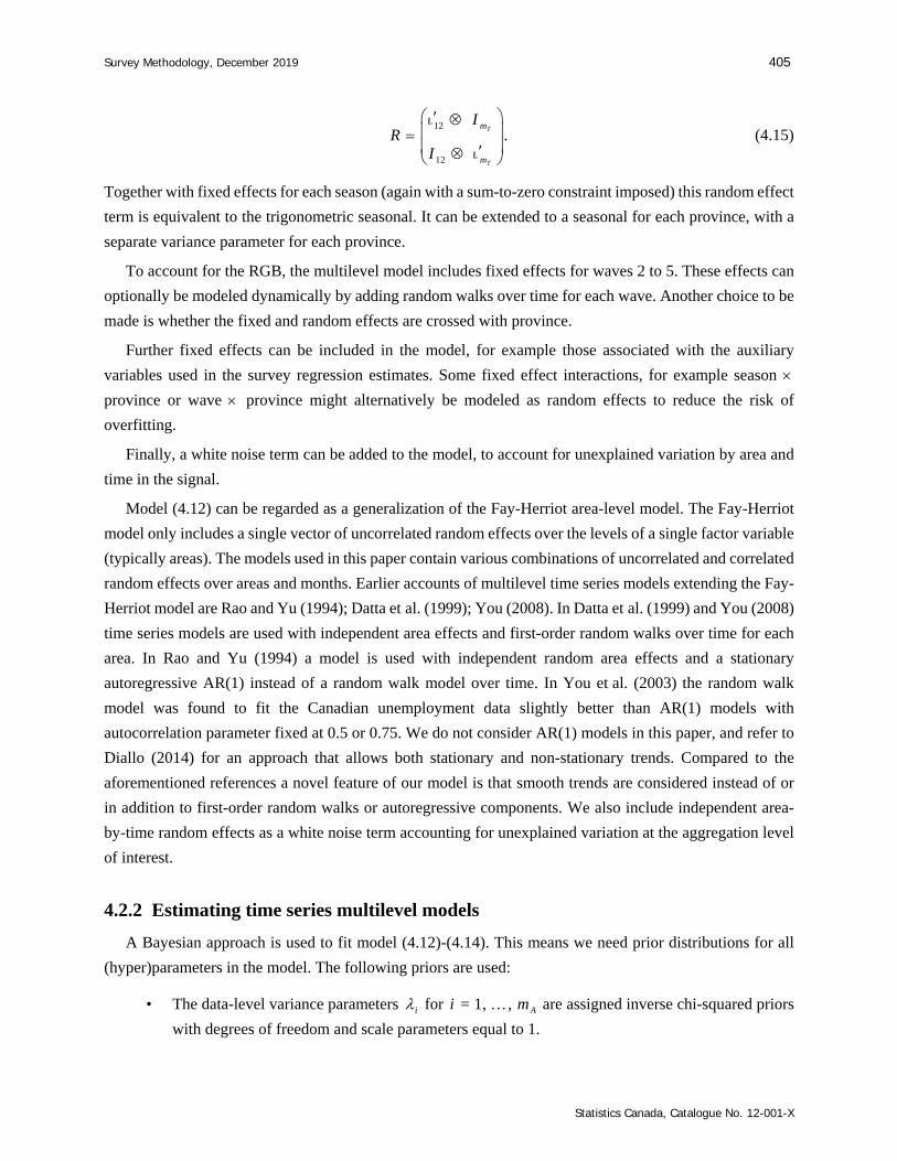
i (4.15)

Together with fixed effects for each season (again with a sum-to-zero constraint imposed) this random effect

term is equivalent to the trigonometric seasonal. It can be extended to a seasonal for each province, with a

separate variance parameter for each province.

To account for the RGB, the multilevel model includes fixed effects for waves 2 to 5. These effects can

optionally be modeled dynamically by adding random walks over time for each wave. Another choice to be

made is whether the fixed and random effects are crossed with province.

Further fixed effects can be included in the model, for example those associated with the auxiliary

variables used in the survey regression estimates. Some fixed effect interactions, for example season

province or wave province might alternatively be modeled as random effects to reduce the risk of

overfitting.

Finally, a white noise term can be added to the model, to account for unexplained variation by area and

time in the signal.

Model (4.12) can be regarded as a generalization of the Fay-Herriot area-level model. The Fay-Herriot

model only includes a single vector of uncorrelated random effects over the levels of a single factor variable

(typically areas). The models used in this paper contain various combinations of uncorrelated and correlated

random effects over areas and months. Earlier accounts of multilevel time series models extending the Fay-

Herriot model are Rao and Yu (1994); Datta et al. (1999); You (2008). In Datta et al. (1999) and You (2008)

time series models are used with independent area effects and first-order random walks over time for each

area. In Rao and Yu (1994) a model is used with independent random area effects and a stationary

autoregressive AR(1) instead of a random walk model over time. In You et al. (2003) the random walk

model was found to fit the Canadian unemployment data slightly better than AR(1) models with

autocorrelation parameter fixed at 0.5 or 0.75. We do not consider AR(1) models in this paper, and refer to

Diallo (2014) for an approach that allows both stationary and non-stationary trends. Compared to the

aforementioned references a novel feature of our model is that smooth trends are considered instead of or

in addition to first-order random walks or autoregressive components. We also include independent area-

by-time random effects as a white noise term accounting for unexplained variation at the aggregation level

of interest.

4.2.2 Estimating time series multilevel models

A Bayesian approach is used to fit model (4.12)-(4.14). This means we need prior distributions for all

(hyper)parameters in the model. The following priors are used:

• The data-level variance parameters i for = 1, , Ai m are assigned inverse chi-squared priors

with degrees of freedom and scale parameters equal to 1.



• The fixed effects are assigned a normal prior with zero mean and fixed diagonal variance matrix

with very large values (1e10).

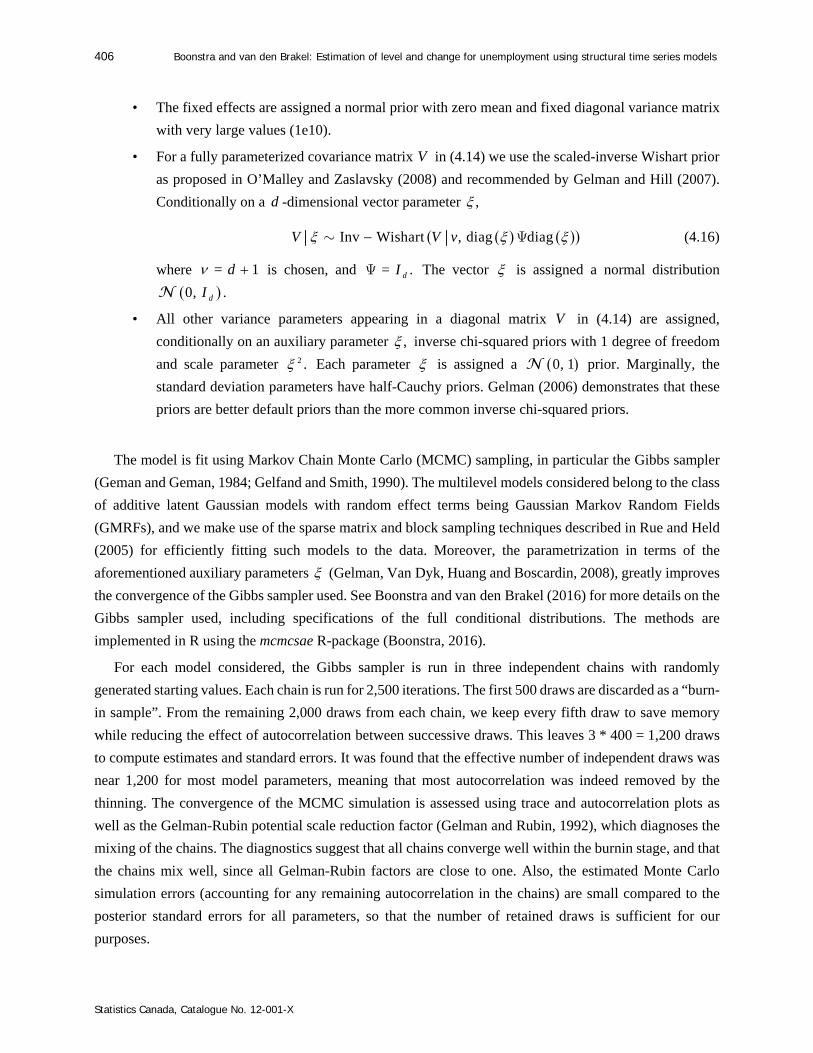
• For a fully parameterized covariance matrix V in (4.14) we use the scaled-inverse Wishart prior

as proposed in O’Malley and Zaslavsky (2008) and recommended by Gelman and Hill (2007).

Conditionally on a d -dimensional vector parameter ,

Inv Wishart , diag diagV V v Y (4.16)

where = 1d is chosen, and = .dIY The vector is assigned a normal distribution

0, .dIN

• All other variance parameters appearing in a diagonal matrix V in (4.14) are assigned,

conditionally on an auxiliary parameter , inverse chi-squared priors with 1 degree of freedom

and scale parameter 2 . Each parameter is assigned a 0, 1N prior. Marginally, the

standard deviation parameters have half-Cauchy priors. Gelman (2006) demonstrates that these

priors are better default priors than the more common inverse chi-squared priors.

The model is fit using Markov Chain Monte Carlo (MCMC) sampling, in particular the Gibbs sampler

(Geman and Geman, 1984; Gelfand and Smith, 1990). The multilevel models considered belong to the class

of additive latent Gaussian models with random effect terms being Gaussian Markov Random Fields

(GMRFs), and we make use of the sparse matrix and block sampling techniques described in Rue and Held

(2005) for efficiently fitting such models to the data. Moreover, the parametrization in terms of the

aforementioned auxiliary parameters (Gelman, Van Dyk, Huang and Boscardin, 2008), greatly improves

the convergence of the Gibbs sampler used. See Boonstra and van den Brakel (2016) for more details on the

Gibbs sampler used, including specifications of the full conditional distributions. The methods are

implemented in R using the mcmcsae R-package (Boonstra, 2016).

For each model considered, the Gibbs sampler is run in three independent chains with randomly

generated starting values. Each chain is run for 2,500 iterations. The first 500 draws are discarded as a “burn-

in sample”. From the remaining 2,000 draws from each chain, we keep every fifth draw to save memory

while reducing the effect of autocorrelation between successive draws. This leaves 3 * 400 = 1,200 draws

to compute estimates and standard errors. It was found that the effective number of independent draws was

near 1,200 for most model parameters, meaning that most autocorrelation was indeed removed by the

thinning. The convergence of the MCMC simulation is assessed using trace and autocorrelation plots as

well as the Gelman-Rubin potential scale reduction factor (Gelman and Rubin, 1992), which diagnoses the

mixing of the chains. The diagnostics suggest that all chains converge well within the burnin stage, and that

the chains mix well, since all Gelman-Rubin factors are close to one. Also, the estimated Monte Carlo

simulation errors (accounting for any remaining autocorrelation in the chains) are small compared to the

posterior standard errors for all parameters, so that the number of retained draws is sufficient for our

purposes.



The estimands of interest can be expressed as functions of the parameters, and applying these functions

to the MCMC output for the parameters results in draws from the posteriors for these estimands. In this

paper we summarize those draws in terms of their mean and standard deviation, serving as estimates and

standard errors, respectively. All estimands considered can be expressed as linear predictors, i.e., as linear

combinations of the model parameters. Estimates and standard errors for the following estimands are

computed:

• Signal: the vector it including all fixed and random effects, except those associated with waves

2 to 5. These correspond to the fitted values X Z v

associated with each fifth row

1, 6, 11, of Y and the design matrices.

• Trend: prediction of the long-term trend. This is computed by only incorporating the trend

components of each model in the linear predictor. For most models considered the trend

corresponds to seasonally adjusted figures, i.e., predictions of the signal with all seasonal effects

removed.

• Growth of trend: the differences between trends at two consecutive months.

5 Results

The results obtained with the state space and multilevel time series representations of the STMs are

described in Subsections 5.1 and 5.2, respectively. First, two discrepancy measures are defined to evaluate

and compare the different models. The first measure is the Mean Relative Bias (MRB), which summarizes

the differences between model estimates and direct estimates averaged over time, as percentage of the latter.

For a given model ,M the MRB i is defined as

.

.

ˆMRB 100%,

Mit itt

i

itt

Y

Y

(5.1)

where .itY are the direct estimates by province and month incorporating the ratio RGB adjustment

mentioned at the end of Section 3. This benchmark measure shows for each province how much the model-

based estimates deviate from the direct estimates. The discrepancies should not be too large as one may

expect that the direct estimates averaged over time are close to the true average level of unemployment. The

second discrepancy measure is the Relative Reduction of the Standard Errors (RRSE) and measures the

percentages of reduction in estimated standard errors between model-based and direct estimates, i.e.,

. .

1 ˆRRSE 100% se se se ,Mi it it it

tT

Y Ym

(5.2)

for a given model .M Here the estimated standard errors for the direct estimates follow from a variance

approximation for . ,itY whereas the model-based standard errors are posterior standard deviations or follow

from the Kalman filter/smoother. Posterior standard deviations, standard errors obtained via the Kalman

filter and standard errors of the direct estimators come from different frameworks and are formally spoken



not comparable. They are used in (5.2) to quantify the reduction with respect to the direct estimator only but

not intended as model selection criteria.

5.1 Results state space models

Ten different state space models are compared. Four different trend models are distinguished. The first

trend component is a smooth trend model without correlations between the domains (4.3), abbreviated as

T1. The second trend model, T2, is a smooth trend model (4.3) with a full correlation matrix for the slope

disturbances (4.9). The third trend component, T3, is a common smooth trend model for all provinces with

eleven local level trend models for the deviation of the domains from this overall trend ((4.10) in

combination with (4.11)). The fourth trend model, T4, is a common smooth trend model for all provinces

with eleven smooth trend models for the deviation of the domains from this overall trend ((4.10) in

combination with (4.3)). In T3 and T4 the province Groningen is taken equal to the overall trend. The

component for the RGB (4.4) can be domain specific (indicated by letter “R” in the model’s name) or chosen

equal for all domains (no “R” in the model’s name). An alternative simplicfication is to assume that RGB

for waves 2, 3, 4 and 5 are equal but domain specific (indicated by “R2”). In a similar way the seasonal

component can be chosen domain specific (indicated by “S”) or taken equal for all domains. All models

share the same component for the survey error, i.e., an AR(1) model with time varying autocorrelation

coefficients for wave 2 through 5 to model the autocorrelation in the survey errors. The following state space

models are compared:

T1SR: Smooth trend model and no correlation between slope disturbances; seasonal and RGB

domain specific.

T2SR: Smooth trend model with a full correlation matrix for the slope disturbances; seasonal and

RGB domain specific.

T2S: Smooth trend model with a full correlation matrix for the slope disturbances; seasonal

domain specific, RGB equal over all domains.

T2R: Smooth trend model with a full correlation matrix for the slope disturbances; seasonal equal

over all domains, RGB domain specific.

T3SR: One common smooth trend model for all domains plus eleven local levels for deviations from

the overall trend; seasonal and RGB domain specific.

T3R: One common smooth trend model for all domains plus eleven local levels for deviations from

the overall trend; seasonal equal over all domains, RGB domain specific.

T3R2: One common smooth trend model for all domains plus eleven local levels for deviations from

the overall trend; seasonal equal over all domains, RGB is domain specific but assumed to

be equal for the four follow-up waves.

T3: One common smooth trend model for all domains plus eleven local levels for deviations from

the overall trend; seasonal and RGB equal over all domains.

T4SR: One common smooth trend model for all domains plus eleven smooth trend models for

deviations from the overall trend; seasonal and RGB domain specific.



T4R: One common smooth trend model for all domains plus eleven smooth trend models for

deviations from the overall trend; seasonal equal over all domains, RGB domain specific.

For all models, the ML estimates for the hyperparameters of the RGB and the seasonals tend to zero,

which implies that these components are time invariant. Also the ML estimates for the variance components

of the white noise of the population domain parameters tend to zero. This component is therefore removed

from model (4.2). The ML estimates for the variance components of the survey errors in the first wave vary

between 0.93 and 1.90. For the follow-up waves, the ML estimates vary between 0.86 and 1.80. The

variances of the direct estimates are pooled over the domains (3.2), which might introduce some bias, e.g.,

underestimation of the variance in domains with high unemployment rates. Scaling the variances of the

survey errors with the ML estimates for 2ip is neccessary to correct for this bias. The ML estimates for the

hyperparameters for the trend components can be found in Boonstra and van den Brakel (2016).

Models are compared using the log likelihoods. To account for differences in model complexity, Akaike

Information Criteria (AIC) and Bayes Information Criteria (BIC) are used, see Durbin and Koopman (2012),

Section 7.4. Results are summarized in Table 5.1. Parsimonious models where the seasonals or RGB are

equal over the domains are preferred by the AIC or BIC criteria. Note, however, that the likelihoods are not

completely comparable between models. To obtain comparable likelihoods, the first 24 months of the series

are ignored in the computation of the likelihood for all models. Some of the likelihoods are nevertheless

odd. For example the likelihood of T2SR is smaller than the likelihood of T2S, although T2SR contains

more model parameters. This is probably the result of large and complex time series models in combination

with relatively short time series, which gives rise to flat likelihood functions. Also from this point of view,

sparse models that avoid over-fitting are still favorable, which is in line with the results of the AIC and BIC

values in Table 5.1.

Table 5.1 AIC and BIC for the state space models

Model log likelihood states hyperparameters AIC BIC T1SR 9,813.82 204 24 -399.41 -390.52 T2SR 9,862.86 204 35 -400.99 -391.68 T2S 9,879.03 160 35 -403.50 -395.90 T2R 9,859.97 83 35 -405.92 -401.32 T3SR 9,855.35 193 24 -401.60 -393.14 T3R 9,851.62 72 24 -406.48 -402.74 T3R2 9,871.65 36 24 -408.82 -406.48 T3 9,881.16 28 24 –409.55 -407.52 T4SR 9,857.47 204 24 -401.23 -392.34 T4R 9,853.65 83 24 -406.11 -401.94

Modeling correlations between slope disturbances of the trend results in a significant model

improvement. Model T1SR, e.g., is nested within T2SR and a likelihood ratio test clearly favours the latter.

For model T2SR it follows that the dynamics of the trends for these 12 domains can be modeled with only

2 underlying common trends, since the rank of the 12 12 covariance matrix equals two. As a result the

full covariance matrix for the slope disturbances of the 12 domains is actually modeled with 23 instead of



78 hyperparameters. This shows that the correlations between the slope disturbances are very strong.

Correlations indeed vary between 1.00 and 0.98. See Boonstra and van den Brakel (2016) for the ML

estimates of the full covariance matrix.

Table 5.2 shows the MRB, defined by (5.1). Models that assume that the RGB is equal over the domains,

i.e., T2S and T3, have large relative biases for some of the domains. Large biases occur in the domains

where unemployment is large (e.g., Groningen) or small (e.g., Utrecht) compared to the national average.

A possible compromise between parsimony and bias is to assume that the RGB is equal for the four follow-

up waves but still domain specific (T3R2). For this model the bias is small, with the exception of Gelderland.

Table 5.2 Mean Relative Bias averaged (5.1) over time (%), per province for state space models

Grn Frs Drn Ovr Flv Gld Utr N-H Z-H Zln N-B Lmb T1SR 1.1 0.5 2.0 -0.2 0.1 3.4 0.1 0.6 1.7 -2.1 0.5 2.1 T2SR 1.2 0.7 2.2 -0.1 0.2 3.5 0.2 0.6 1.7 -2.1 0.5 2.1 T2S -3.1 3.1 0.7 0.9 -4.4 2.8 2.4 0.8 0.5 1.7 1.8 1.5 T2R 0.9 0.8 1.8 -0.2 -0.4 3.4 0.1 0.6 1.7 -1.6 0.6 2.2 T3SR 0.8 0.6 2.0 -0.2 -0.3 3.5 0.3 0.5 1.7 -2.0 0.6 2.0 T3R2 -0.1 1.3 2.1 -0.6 -0.8 3.6 0.9 0.6 1.5 -1.1 1.0 1.2 T3R 0.5 0.7 1.8 -0.2 -0.8 3.5 0.3 0.5 1.6 -1.5 0.7 2.1 T3 -4.0 2.5 0.1 0.9 -5.0 2.8 2.3 0.7 0.6 2.5 2.0 1.3 T4SR 0.8 0.7 2.1 -0.2 -0.0 3.5 0.2 0.6 1.7 -1.9 0.5 2.1 T4R 0.6 0.7 1.8 -0.2 -0.6 3.4 0.1 0.6 1.7 -1.3 0.7 2.1

In Figure 5.1 the smoothed trends and standard errors of models T1SR, T2SR and T2S are compared.

The month-to-month development of the trend and the standard errors for these three models are compared

in Figure 5.2. The smoothed trends obtained with the common trend model are slightly more flexible

compared to a model without correlation between the slope disturbances. This is clearly visible in the month-

to-month change of the trends. Modeling the correlation between slope disturbances clearly reduces the

standard error of the trend and the month-to-month change of the trend. Assuming that the RGB is equal for

all domains (model T2S) affects the level of the trend and further reduces the standard error, mainly since

the number of state variables are reduced. The difference between the trend under T2SR and T2S is a level

shift. This follows from the month-to-month changes of the trend under model T2SR and T2S, which are

exactly equal. According to AIC and BIC the reduction of the number of state variables by assuming equal

RGB for all domains is an improvement of the model. In this application, however, interest is focused on

the model fit for the separate domains. Assuming that the RGB is equal over all domains is on average

efficient for overall goodness of fit measures, like AIC and BIC, but not necessarily for all separate domains.

The bias introduced in the trends of some of the domains by taking the RGB equal over the domains is

undesirable.

In Figure 5.3 the smoothed trends and standard errors of models T2SR, T3SR and T4SR are compared.

The month-to-month developments of the trend and the standard errors can be found in Boonstra and

van den Brakel (2016). The trends obtained with one overall smooth trend plus eleven trends for the domain



deviations of the overall trend resemble trends obtained with the common trend model. In this application

the dynamics based on the two common trends of model T2SR are reasonably well approximated by the

alternative trends of models T3SR and T4SR. This is an empirical finding that may not generalize to other

situations, particularly when more common factors are required. The common trend model, however, has

the smallest standard errors for the trend. Furthermore, the trends under the model with a local level for the

domain deviations from the overall trend are in some domains more volatile compared to the other two

models. This is most obvious in the month-to-month changes of the trend. It is a general feature for trend

models with random levels to have more volatile trends, see Durbin and Koopman (2012), Chapter 3. The

more flexible trend model of T3 also results in a higher standard error of the month-to-month changes.

Assuming that the seasonals are equal for all domains is another way of reducing the number of state

variables and avoid over-fitting of the data. This assumption does not affect the level of the trend since the

MRB is small (see Table 5.2) and results in a significant improvement of the model according to AIC and

BIC. Particularly if interest is focused on trend estimates, some bias in the seasonal patterns is acceptable

and a model with a trend based on T2, or T4, with the seasonal component assumed equal over the domains,

might be a good compromise between a model that accounts sufficiently for differences between domains

and model parsimony to avoid over-fitting of the data.

Model T3 is the most parsimonious model that is the best model according to AIC and BIC. Particularly

the assumption of equal RGB results in biased trend estimates in some of the domains (see Table 5.2). See

Boonstra and van den Brakel (2016) for a comparison of the trend and the month-to-month development of

the trend of models T2R, T3 and T4R. Assuming that the seasonals are equal over the domains, results in a

less pronounced seasonal pattern. See Boonstra and van den Brakel (2016) for a comparison of the signals

for models T2SR and T2R.

In Boonstra and van den Brakel (2016) results for year-to-year change of the trends under models T2R

and T3R2 are included. Time series estimates for year-to-year change are very stable and precise and greatly

improve the direct estimates for year-to-year change.

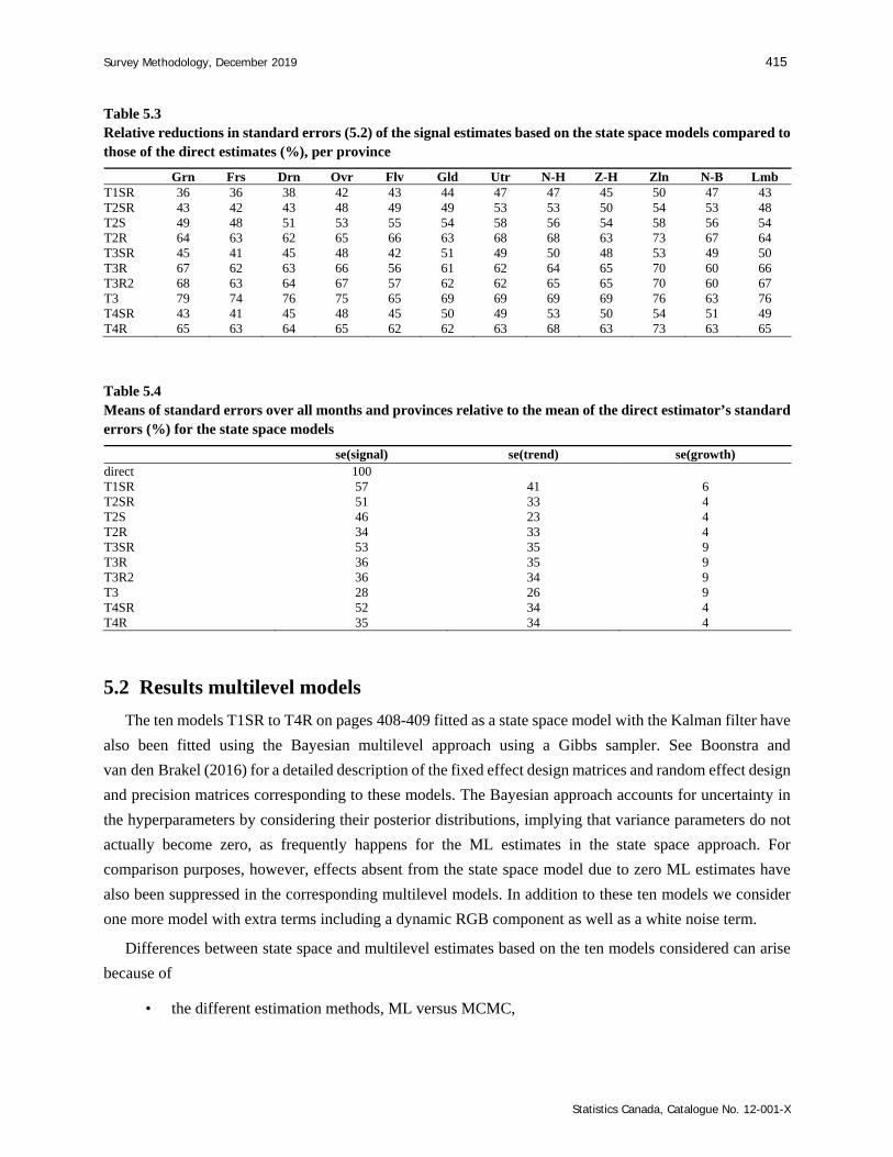
Table 5.3 shows the RRSE, defined by (5.2), for the ten state space models. Recall that the RRSE

quantifies the reduction with respect to the direct estimator and is not intended as a model selection criterion.

Table 5.4 contains the averages of standard errors for signal, trend, and growth (month-to-month differences

of trend). The average is taken over all months and provinces. Modeling the correlation between the trends

explicitly (T2) or implicitly (T3 or T4) reduces the standard errors for the trend and signal significantly. The

time series modeling approach is particularly appropriate to estimate month-to-month changes through the

trend component. The precision of the month-to-month changes, however, strongly depends on the choice

of the trend model. A local level trend model (T3) results in more volatile trends and has a clearly larger

standard error for the month-to-month change. Parsimonious models where RGB or the seasonal

components are assumed equal over the domains result in further strong standard error reductions at the cost

of introducing bias in the trend or the seasonal patterns.



Figure 5.1 Comparison of direct estimates and smoothed trend estimates for three models (left) and their estimated standard errors (right).

Fra

ctio

n u

nem

plo

yed

Flevoland, estimates Flevoland, standard errors

0.08

0.06

0.04

0.02

0.04

0.03

0.02

0.04

0.03

Zeeland, estimates Zeeland, standard errors

series direct STS T1SR STS T2SR STS T2S

Zuid-Holland, estimates Zuid-Holland, standard errors

Jan Jan Jan Jan Jan Jan Jan Jan Jan Jan 2004 2005 2006 2007 2008 2004 2005 2006 2007 2008

month

0.008

0.006

0.004

0.002

0.006

0.004

0.002

0.0025

0.0020

0.0015

0.0010

0.0005



Figure 5.2 Comparison of smoothed month-to-month developments (left) and their standard errors (right).

Fra

ctio

n u

nem

plo

yed


0.0015

0.0010

0.0005

0.0000

-0.0005

-0.0010

-0.0015

4e-04

0e+00

-4e-04

5e-04

0e+00

-5e-04



series STS T1SR STS T2SR STS T2S


month

7e-04

6e-04

5e-04

4e-04

3e-04

4e-04

3e-04

2e-04

0.00030

0.00025

0.00020



Figure 5.3 Comparison of direct estimates and smoothed trend estimates for three models (left) and their estimated standard errors (right).

Fra

ctio

n u

nem

plo

yed


0.08

0.06

0.04

0.02

0.04

0.03

0.02

0.04

0.03


series direct STS T2SR STS T3SR STS T4SR


month

0.008

0.006

0.004

0.002

0.006

0.004

0.002

0.0025

0.0020

0.0015

0.0010




Table 5.3 Relative reductions in standard errors (5.2) of the signal estimates based on the state space models compared to those of the direct estimates (%), per province

Grn Frs Drn Ovr Flv Gld Utr N-H Z-H Zln N-B Lmb T1SR 36 36 38 42 43 44 47 47 45 50 47 43 T2SR 43 42 43 48 49 49 53 53 50 54 53 48 T2S 49 48 51 53 55 54 58 56 54 58 56 54 T2R 64 63 62 65 66 63 68 68 63 73 67 64 T3SR 45 41 45 48 42 51 49 50 48 53 49 50 T3R 67 62 63 66 56 61 62 64 65 70 60 66 T3R2 68 63 64 67 57 62 62 65 65 70 60 67 T3 79 74 76 75 65 69 69 69 69 76 63 76 T4SR 43 41 45 48 45 50 49 53 50 54 51 49 T4R 65 63 64 65 62 62 63 68 63 73 63 65

Table 5.4 Means of standard errors over all months and provinces relative to the mean of the direct estimator’s standard errors (%) for the state space models

se(signal) se(trend) se(growth) direct 100 T1SR 57 41 6 T2SR 51 33 4 T2S 46 23 4 T2R 34 33 4 T3SR 53 35 9 T3R 36 35 9 T3R2 36 34 9 T3 28 26 9 T4SR 52 34 4 T4R 35 34 4

5.2 Results multilevel models

The ten models T1SR to T4R on pages 408-409 fitted as a state space model with the Kalman filter have

also been fitted using the Bayesian multilevel approach using a Gibbs sampler. See Boonstra and

van den Brakel (2016) for a detailed description of the fixed effect design matrices and random effect design

and precision matrices corresponding to these models. The Bayesian approach accounts for uncertainty in

the hyperparameters by considering their posterior distributions, implying that variance parameters do not

actually become zero, as frequently happens for the ML estimates in the state space approach. For

comparison purposes, however, effects absent from the state space model due to zero ML estimates have

also been suppressed in the corresponding multilevel models. In addition to these ten models we consider

one more model with extra terms including a dynamic RGB component as well as a white noise term.

Differences between state space and multilevel estimates based on the ten models considered can arise

because of

• the different estimation methods, ML versus MCMC,



• the different modeling of survey errors. In the multilevel models the survey errors’ covariance

matrix is taken to be =1= Ami i i with i the covariance matrix of estimated design variances

for the initial estimates for province ,i and i scaling factors, one for each province. In the state

space models the survey errors are allowed to depend on more parameters though eventually an

AR(1) model is used to approximate these dependencies,

• the slightly different parameterizations of the trend components. For the trend in model T3, for

example, the province of Groningen is singled out by the state space model used, because no local

level component is added for that province.

The estimates and, to a lesser extent, the standard errors based on the multilevel models are quite similar

to the results obtained with the state space models. We show this only for the smoothed signals of model

T2R in Figure 5.4, as the qualitative differences between state space and multilevel results are quite

consistent over all models. More comparisons for signals, trends and month-to-month developments for

models T2R and T3R2 can be found in Boonstra and van den Brakel (2016).

The small differences between the state space and multilevel signal estimates are due to slightly more

flexible trends in the estimated multilevel models. Larger differences can be seen in the standard errors of

the signal: the multilevel models yield almost always larger standard errors for provinces with high

unemployment levels (Flevoland and Zuid-Holland in the figure), whereas for provinces with smaller

unemployment levels (e.g., Zeeland) the differences are somewhat less pronounced.

The larger flexibility of the multilevel model trends is most likely due to the relatively large uncertainty

about the variance parameters for the trend, which is accounted for in the Bayesian multilevel approach but

ignored in the ML approach for the state space models. The posterior distributions for the trend variance

parameters are also somewhat right-skewed. The posterior means for the standard deviations are always

larger than the ML estimates for the corresponding hyperparameters of the state space models (compare

Table 2 and Table 8 in Boonstra and van den Brakel (2016)). For the models with trend T2, i.e., with a fully

parametrized covariance matrix over provinces, the multilevel models show positive correlations among the

provinces, as do the state space ML estimates, but the latter are much more concentrated near 1, whereas

the posterior means for correlations in the corresponding multilevel model T2SR are all between 0.45

and 0.8.

Table 5.5 contains values of the DIC model selection criterion (Spiegelhalter, Best, Carlin and

van der Linde, 2002), the associated effective number of model parameters eff ,p and the posterior mean of

the log-likelihood. The parsimonious model T3 is selected as the most favourable model by the DIC

criterion. So in this case the DIC criterion selects the same model as the AIC and BIC criteria do for the

state space models. An advantage of DIC is that it uses an effective number of model parameters depending

on the size of random effects, instead of just the number of model parameters used in AIC/BIC. That said,

the numbers effp are in line with the totals of the numbers of states and hyperparameters in Table 5.1 for

the state space models.



Figure 5.4 Comparison between smoothed signals (left) and their standard errors (right) obtained using state space (STS) model T2R and the corresponding multilevel model.

Fra

ctio

n u

nem

plo

yed


0.08

0.06

0.04

0.02

0.04

0.03

0.02

0.04

0.03


Signal T2R direct STS multilevel


month

0.008

0.006

0.004

0.002

0.006

0.004

0.002

0.0025

0.0020

0.0015

0.0010




Table 5.5 DIC, effective number of model parameters and posterior mean of log likelihood

DIC effp mean llh

T1SR -29,054 255 14,655 T2SR -29,076 235 14,656 T2S -29,129 196 14,662 T2R -29,164 118 14,641 T3SR -29,081 242 14,662 T3R -29,174 126 14,650 T3R2 -29,217 94 14,655 T3 -29,230 82 14,656 T4SR -29,084 228 14,656 T4R -29,170 109 14,640

As was the case for the state space models, the parsimonious model T3 comes with larger average bias

over time for the provinces Groningen and Flevoland, which have the highest rates of unemployment. Model

T3R2 has much smaller average biases for Groningen and Flevoland and since its DIC value is not that

much higher than for model T3, model T3R2 seems to be a good compromise between models T3 and T3R,

being more parsimonious than T3R and respecting provincial differences better than model T3.

Table 5.6 contains the average standard errors for signal, trend and month-to-month differences in the

trend, in comparison to the average for the direct estimates. The average is taken over all months and

provinces. The results are again similar to the results obtained with the state space models, see Table 5.4,

although especially the standard errors of month-to-month changes are larger under the multilevel models.

Table 5.6 Means of standard errors over all months and provinces relative to the mean of the direct estimator’s standard errors (%) for the multilevel time series models

se(signal) se(trend) se(growth) direct 100 T1SR 55 41 8 T2SR 52 37 6 T2S 49 33 7 T2R 39 38 6 T3SR 53 38 15 T3R 39 38 15 T3R2 39 38 15 T3 34 32 15 T4SR 51 36 6 T4R 37 36 6

Finally, a multilevel model based on model T3R2 but with additional random effects has been fitted to

the data. This extended model includes a white noise term, the balanced dummy seasonal (equivalent to the

trigonometric seasonal), and a dynamic RGB component. These components were seen to be absent or time

independent in the state space approach due to zero ML hyperparameter estimates, and therefore were also



not included in the multilevel models considered so far. In addition, the extended multilevel model includes

season by province random effects, as a compromise between fixed provincial seasonal effects and no such

interaction effects at all. More details and figures comparing the estimation results from this extended model

to those from multilevel models T3R2 and T3SR can be found in Boonstra and van den Brakel (2016). It

was found that most additional random effects were small so that the estimates based on the extended model

are quite close to the estimates based on model T3R2, and the estimated standard errors are only slightly

larger than those for model T3R2. A DIC value of -29,260 was found, well below the DIC value for model

T3R2. This improvement in DIC was seen to be almost entirely due to the dynamic RGB component.

Apparently, modeling the RGB as time-dependent results in a better fit. This seems to be in line with the

temporal variations in differences between first wave and follow-up wave survey regression estimates,

visible from Figure 3 in Boonstra and van den Brakel (2016).

6 Discussion

A time series small area estimation model has been applied to a large amount of survey data, comprising

6 years of Dutch LFS data, to estimate monthly unemployment fractions for 12 provinces over this period.

Two different estimation approaches for structural time series models (STM) are applied and compared.

The first one is a state space approach using a Kalman filter, where the unknown hyperparameters are

replaced by their ML estimates. The second one is a Bayesian multilevel time series approach, using a Gibbs

sampler.

The time series models that do not account for cross-sectional correlations and borrow strength over time

only, already show a major reduction of the standard errors compared to the direct estimates. A further small

decrease of the standard errors is obtained by borrowing strength over space through cross-sectional

correlations in the time series models. Another great advantage of the time series model approach concerns

the estimation of change. Under the multilevel model estimates of change and their standard errors can be

easily computed, especially when the model fit is in the form of an MCMC simulation. Under the state space

approach, estimates of change follow directly from the Kalman filter recursion by keeping the required state

variables from the past in the state vector. The desired estimate for change, including its standard error,

follows from the contrast of the specific state variables. Month-to-month and year-to-year change of

monthly data are very stable and precise, which is a consequence of the strong positive correlation between

level estimates. However, the stability of the estimates of change strongly depends on the choice of the trend

model. Local level models result in more volatile trend estimates and thus also more volatile estimates of

change and naturally have a higher standard error compared to smooth trend models.

In this paper different trend models are considered that model correlation between domains with the

purpose to borrow strength over time and space. The most complex approach is to specify a full covariance

matrix for the disturbance terms of the trend component. One way to construct parsimonious models is to

take advantage of cointegration. In the case of strong correlation between domains the covariance matrix



will be of reduced rank, which means that the trends of the Am domains are driven by less than Am common

trends. In this application two common trends are sufficient to model the dynamics of the twelve provinces,

resulting in a strong reduction of the number of hyperparameters required to model the cross-sectional

correlations between the domains. In order to further reduce the number of state and hyperparameters,

alternative trend models are considered that implicitly account for cross-sectional correlations. Under this

approach all domains share an overall trend. Each domain has a domain-specific trend to account for the

deviation from the overall trend. This can be seen as a simplified form of a common trend model. In this

application the alternative trend model results in comparable estimates for the trends and standard errors.

So this approach might be a practical attractive alternative for common trend models. For example if the

number of domains is large or the number of common factors is larger, then the proposed trend models are

less complex compared to general common trend models. More research into the statistical properties of

these alternative trend models is necessary for better understanding the implied covariance structures.

Several differences between the time series multilevel models fitted in an hierarchical Bayesian

framework and state space models fitted with the Kalman filter with a frequentist approach can be observed.

Within the multilevel Bayesian framework different STMs are compared using DIC as a formal model

selection criterion. Since the state space models are fitted in a frequentist framework, STMs are compared

with AIC or BIC. An advantage of the DIC criterion used in the Bayesian multilevel approach is that it uses

the effective number of degrees of freedom as a penalty for model complexity. This implies that the penalty

for a random effect increases with the size of the variance components of this random factor and varies

between zero if the variance component equals zero and the number of levels of this factor if the variance

component tends to infinity. The penalty in AIC or BIC for a random component always equals one,

regardless the size of its variance component and therefore does not account properly for model complexity.

Note that for multilevel models fitted in a frequentist framework the so-called conditional AIC is proposed

(Vaida and Blanchard, 2005) where the penalty for model complexity is also based on the effective degrees

of freedom. In this case the penalty for a random effect increases as the size of its variance component

increases in a similar way as with the DIC. For state space models fitted in a frequentist framework such

model selection criteria seem less readily available.

A difference between the multilevel models and state space models is that under the former model

components are more often found to be time varying while under the state space approach most components,

with the exception of the trend, are estimated as time invariant. This is a result of the method of model

fitting. Under the frequentist approach applied to the state space models, ML estimates for many

hyperparameters are on the border of the parameter space, i.e., zero for variance components and one for

correlations between slope disturbance terms. Under the hierarchical Bayesian approach the entire

distribution of the (co)variance parameters is simulated resulting in mean values for these hyperparameters

that are never exactly on the border of the parameter space, e.g., always positive in the case of variance

components. A consequence of this feature is that the variances of the trend hyperparameters are higher and

that the covariances between the trend disturbances are smaller than one under the hierarchical Bayesian



approach. Another remarkable observation is that the DIC prefers models with time varying RGB and time

varying seasonal components as well as a white noise term for the population parameter. This results in this

application in models with a higher degree of complexity under the hierarchical Bayesian multilevel models

compared to the state space models fitted in a frequentist approach. Differences in estimates for the trend

and the signals are, however, small.

An advantage of the hierarchical Bayesian approach is that the standard errors of the domain predictions

account for the uncertainty about the hyperparameters. As a result the standard errors obtained under the

hierarchical Bayesian approach of comparable models are slightly higher and less biased compared to the

state space approach. For the state space approach several bootstrap methods are available to account for

hyperparameter uncertainty (Pfeffermann and Tiller, 2005) but these methods significantly increase the

computational cost.

From a computational point of view there are some differences between the methods too. The Kalman

filter approach applied to state space models can be used online, producing new filtered estimates by

updating previous predictions when data for a new month arrives and is from that point of view

computationally very efficient. The numerical optimization procedure for ML estimation of the

hyperparameters, on the other hand, can be cumbersome for large multivariate models if the number of

hyperparameters is large. The Gibbs sampler multilevel approach used here produces estimates for the

whole time series at once. It must be re-estimated completely when data for a new month arrives. However,

due to the use of sparse matrices and redundant parameterization the multilevel approach is quite

competitive computationally, see also Knorr-Held and Rue (2002). An advantage of the simultaneous

multilevel estimation is that constraints over time can easily be imposed. For example, imposing sum-to-

zero constraints over time allows to include local level provincial trends for all provinces in addition to a

global smooth trend with no resulting identification issues.

In this application there is a preference for the time series multilevel models in the hierarchical Bayesian

framework. One reason is the relatively simple way the DIC criterion can be computed, which better

accounts for model complexity than AIC or BIC. Also, the Gibbs sampler under the Bayesian approach is

better suited to fit complex multivariate STMs with large numbers of hyperparameters. In addition, the

standard errors for the domain predictions obtained under the multilevel models account for the uncertainty

about the hyperparameters, also in a straightforward way.

The time series estimates are quite smooth, and a more thorough model evaluation is necessary to find

out whether that is appropriate or whether the time series model underfits the unemployment data or is open

to improvement in other ways. There are many ways in which the time series SAE model may be extended

to further improve the estimates and standard errors. For example, it may be an improvement to use a

logarithmic link function in the model formulation as in You (2008). Effects would then be multiplicative

instead of additive. Another possible improvement would come from a more extensive modeling of the

sampling variances (You and Chapman, 2006; You, 2008; Gómez-Rubio, Best, Richardson, Li and Clarke,

2010). The models can also be improved by including additional auxiliary information at the province by



month level, for instance registered unemployment. In Datta et al. (1999) similar effects associated with

unemployment insurance are modeled as varying over areas, although not over time.

Acknowledgements

The views expressed in this paper are those of the authors and do not necessarily reflect the policy of

Statistics Netherlands. This work was funded by the European Union under grant no. 07131.2015.001-

2015.257. We are grateful to the unknown reviewers and the Associate Editor for careful reading of a former

draft of this manuscript and providing useful comments.

References

Andrieu, C., Poucet, R. and Holenstein, R. (2010). Particle markov chain monte carlo methods. Journal of the Royal Statistical Society, Series B, 72, 269-342.

Bailar, B.A. (1975). The effects of rotation group bias on estimates from panel surveys. Journal of the

American Statistical Association, 70, 349, 23-30. Battese, G.E., Harter, R.M. and Fuller, W.A. (1988). An error-components model for prediction of county

crop areas using survey and satellite data. Journal of the American Statistical Association, 83, 401, 28-36.

Bollineni-Balabay, O., van den Brakel, J., Palm, F. and Boonstra, H.J. (2016). Multilevel hierarchical

bayesian vs. state-space approach in time series small area estimation; the dutch travel survey. Technical Report 2016-03, https://www.cbs.nl/en-gb/our-services/methods/papers, Statistics Netherlands.

Boonstra, H.J. (2016). mcmcsae: MCMC Small Area Estimation. R package version 0.7, available on request

from the author. Boonstra, H.J., and van den Brakel, J. (2016). Estimation of level and change for unemployment using

multilevel and structural time-series models. Technical Report 2016-10, https://www.cbs.nl/en-gb/our-services/methods/papers, Statistics Netherlands.

Chan, J.C.C., and Jeliazkov, I. (2009). Efficient simulation and integrated likelihood estimation in state

space models. International Journal of Mathematical Modelling and Numerical Optimisation, 1, 101-120.

Datta, G.S., Lahiri, P., Maiti, T. and Lu, K.L. (1999). Hierarchical bayes estimation of unemployment rates

for the states of the U.S. Journal of the American Statistical Association, 94, 448, 1074-1082. Diallo, M.S. (2014). Small Area Estimation Under Skew-Normal Nested Error Models. PhD thesis, School

of Mathematics and Statistics, Carleton University, Ottawa, Canada. Doornik, J.A. (2009). An Object-oriented Matrix Programming Language Ox 6. Timberlake Consultants

Press.



Durbin, J., and Koopman, S.J. (2012). Time Series Analysis by State Space Methods. Oxford University Press.

Fay, R.E., and Herriot, R.A. (1979). Estimates of income for small places: An application of James-Stein

procedures to census data. Journal of the American Statistical Association, 74, 366, 269-277. Gelfand, A.E., and Smith, A.F.M. (1990). Sampling based approaches to calculating marginal densities.

Journal of the American Statistical Association, 85, 398-409. Gelman, A. (2006). Prior distributions for variance parameters in hierarchical models. Bayesian Analysis,

1, 3, 515-533. Gelman, A., and Hill, J. (2007). Data Analysis Using Regression and Multilevel/Hierarchical Models.

Cambridge University Press. Gelman, A., and Rubin, D.B. (1992). Inference from iterative simulation using multiple sequences.

Statistical Science, 7, 4, 457-472. Gelman, A., Van Dyk, D.A., Huang, Z. and Boscardin, W.J. (2008). Using redundant parameterizations to

fit hierarchical models. Journal of Computational and Graphical Statistics, 17, 1, 95-122. Geman, S., and Geman, D. (1984). Stochastic relaxation, gibbs distributions and the bayesian restoration of

images. IEEE Trans. Pattn Anal. Mach. Intell., 6, 721-741. Gómez-Rubio, V., Best, N., Richardson, S., Li, G. and Clarke, P. (2010). Bayesian statistics for small area

estimation. Technical Report http://www.bias-project.org.uk/research.htm. Harvey, A.C. (2006). Seasonality and unobserved components models: an overview. Technical Report ISSN

1725-4825, Conference on seasonality, seasonal adjustment and their implications for shortterm analysis and forecasting, 10-12 May 2006, Luxembourg.

Kish, L. (1965). Survey Sampling. Wiley. Knorr-Held, L., and Rue, H. (2002). On block updating in markov random field models for disease mapping.

Scandinavian Journal of Statistics, 29, 4, 597-614. Koopman, S.J., Harvey, A.C., Doornik, J.A. and Shephard, A. (1999). STAMP: Structural Time Series

Analyser, Modeller and Predicter. Timberlake Consultants, Press London. Koopman, S.J., Shephard, A. and Doornik, J.A. (1999). Statistical algorithms for models in state-space form

using ssfpack 2.2. Econometrics Journal, 2, 113-166. Koopman, S.J., Shephard, A. and Doornik, J.A. (2008). Ssfpack 3.0: Statistical algorithms for models in

state-space form. Timberlake Consultants, Press London. Krieg, S., and van den Brakel, J.A. (2012). Estimation of the monthly unemployment rate for six domains

through structural time series modelling with cointegrated trends. Computational Statistics and Data Analysis, 56, 2918-2933.

McCausland, W.J., Miller, S. and Pelletier, D. (2011). Simulation smoothing for state-space models: A

computational efficiency analysis. Computational Statistics and Data Analysis, 55, 199-212.



O’Malley, A.J., and Zaslavsky, A.M. (2008). Domain-level covariance analysis for multilevel survey data with structured nonresponse. Journal of the American Statistical Association, 103, 484, 1405-1418.

Pfeffermann, D. (1991). Estimation and seasonal adjustment of population means using data from repeated

surveys. Journal of Business & Economic Statistics, 163-175. Pfeffermann, D., and Burck, L. (1990). Robust small area estimation combining time series and cross-

sectional data. Survey Methodology, 16, 2, 217-237. Paper available at https://www150.statcan.gc.ca/n1/en/pub/12-001-x/1990002/article/14534-eng.pdf.

Pfeffermann, D., and Tiller, R. (2005). Bootstrap approximation to prediction mse for state-space models

with estimated parameters. Journal of Time Series Analysis, 26, 893-916. Pfeffermann, D., and Tiller, R. (2006). Small area estimation with state-space models subject to benchmark

constraints. Journal of the American Statistical Association, 101, 1387-1397. Piepho, H.-P., and Ogutu, J.O. (2014). Simple state-space models in a mixed model framework. The

American Statistician, 61, 3, 224-232. Proietti, T. (2000). Comparing seasonal components for structural time series models. International Journal

of Forecasting, 16, 247-260. Rao, J.N.K., and Molina, I. (2015). Small Area Estimation. Wiley-Interscience. Rao, J.N.K., and Yu, M. (1994). Small area estimation by combining time series and cross-sectional data.

The Canadian Journal of Statistics, 22, 511-528. Rue, H., and Held, L. (2005). Gaussian Markov Random Fields: Theory and Applications. Chapman and

Hall/CRC. Ruiz-Cárdenas, R., Krainski, E.T. and Rue, H. (2012). Direct fitting of dynamic models using integrated

nested laplace approximations - inla. Computational Statistics and Data Analysis, 56, 1808-1828. Särndal, C.-E., Swensson, B. and Wretman, J. (1992). Model Assisted Survey Sampling. Springer. Spiegelhalter, D.J., Best, N.G. Carlin, B.P. and van der Linde, A. (2002). Bayesian measures of model

complexity and fit. Journal of the Royal Statistical Society B, 64, 4, 583-639. Vaida, F., and Blanchard, S. (2005). Conditional akaike information for mixed-effects models. Biometrika,

95, 2, 351-370. van den Brakel, J.A., and Krieg, S. (2009). Estimation of the monthly unemployment rate through structural

time series modelling in a rotating panel design. Survey Methodology, 35, 2, 177-190. Paper available at https://www150.statcan.gc.ca/n1/en/pub/12-001-x/2009002/article/11040-eng.pdf.

van den Brakel, J.A., and Krieg, S. (2015). Dealing with small sample sizes, rotation group bias and

discontinuities in a rotating panel design. Survey Methodology, 41, 2, 267-296. Paper available at https://www150.statcan.gc.ca/n1/en/pub/12-001-x/2015002/article/14231-eng.pdf.

van den Brakel, J.A., and Krieg, S. (2016). Small area estimation with state-space common factor models

for rotating panels. Journal of the Royal Statisitcal Society, 179, 763-791.



Woodruff, R. (1966). Use of a regression technique to produce area breakdowns of the monthly national estimates of retail trade. Journal of the American Statistical Association, 61, 314, 496-504.

You, Y. (2008). An integrated modeling approach to unemployment rate estimation for sub-provincial areas

of Canada. Survey Methodology, 34, 1, 19-27. Paper available at https://www150.statcan.gc.ca/n1/en/pub/12-001-x/2008001/article/10614-eng.pdf.

You, Y., and Chapman, B. (2006). Small area estimation using area level models and estimated sampling

variances. Survey Methodology, 32, 1, 97-103. Paper available at https://www150.statcan.gc.ca/n1/en/pub/12-001-x/2006001/article/9263-eng.pdf.

You, Y., Rao, J.N.K. and Gambino, J. (2003). Model-based unemployment rate estimation for the Canadian

Labour Force Survey: A hierarchical Bayes approach. Survey Methodology, 29, 1, 25-32. Paper available at https://www150.statcan.gc.ca/n1/en/pub/12-001-x/2003001/article/6602-eng.pdf.

estimation of level and change for unemployment using

Documents