estimation of morphing airfoil shapes and...

ESTIMATION OF MORPHING AIRFOIL SHAPES

AND AERODYNAMIC LOADS USING

ARTIFICIAL HAIR SENSORS

by

NATHAN SCOTT BUTLER

WEIHUA SU, COMMITTEE CHAIR

SEMIH OLCMEN

HWAN-SIK YOON

A THESIS

Submitted in partial fulfillment of the requirements for

the degree of Master of Science in the Department of

Aerospace Engineering and Mechanics

in the Graduate School of

The University of Alabama

TUSCALOOSA, ALABAMA

2015

Copyright Nathan Scott Butler 2015

ALL RIGHTS RESERVED

ii

ABSTRACT

An active area of research in adaptive structures focuses on the use of continuous wing

shape changing methods as a means of replacing conventional discrete control surfaces and

increasing aerodynamic efficiency. Although many shape-changing methods have been used

since the beginning of heavier-than-air flight, the concept of performing camber actuation on a

fully-deformable airfoil has not been widely applied. A fundamental problem of applying this

concept to real-world scenarios is the fact that camber actuation is a continuous, time-dependent

process. Therefore, if camber actuation is to be used in a closed-loop feedback system, one must

be able to determine the instantaneous airfoil shape, as well as the aerodynamic loads, in real

time. One approach is to utilize a new type of artificial hair sensors (AHS) developed at the Air

Force Research Laboratory (AFRL) to determine the flow conditions surrounding deformable

airfoils. In this study, AHS measurement data will be simulated by using the flow solver XFoil,

with the assumption that perfect data with no noise can be collected from the AHS

measurements. Such measurements will then be used in an artificial neural network (ANN) based

process to approximate the instantaneous airfoil camber shape, lift coefficient, and moment

coefficient at a given angle of attack.

Additionally, an aerodynamic formulation based on the finite-state inflow theory has

been developed to calculate the aerodynamic loads on thin airfoils with arbitrary camber

deformations. Various aerodynamic properties approximated from the AHS/ANN system will be

compared with the results of the finite-state inflow aerodynamic formulation in order to validate

the approximation approach.

iii

DEDICATION

This thesis is dedicated to everyone who helped guide me through the many difficulties

of creating this manuscript. I owe a special thanks to my family and close friends who stood by

me not only throughout the time taken to complete this research, but also throughout all my years

of education thus far. Without their support none of this would be possible.

iv

LIST OF ABBREVIATIONS AND SYMBOLS

cross-sectional area of hair sensor

coefficient of pressure

neural network hidden unit

lift force

generalized aerodynamic loads

aerodynamic center pitching moment

mid-chord pitching moment

maximum data capability of neural network

neural network output

neural network input

Legendre polynomials of the first kind

pressure gradient

normalized local velocity limit

finite-state mode magnitude expansion vector

semi-chord length

sectional lift coefficient

sectional pitching moment coefficient

sectional mid-chord drag force

location of elastic axis

v

reversed flow parameter

elastic camber deformation

free-stream velocity

velocity expansion vector

acceleration expansion vector

free-stream velocity or airfoil translational velocity

plunging velocity

plunging acceleration

pitching velocity

pitching acceleration

Δ hair sensor deflection

camber deformation with added elastic deformation

bound vorticity

downwash due to free vorticity

air density

Glauert variable (angle)

reference point location

vi

ACKNOWLEDGEMENTS

I am pleased to have this opportunity to thank the many colleagues, friends, and faculty

members who have helped me with this research work. I am most indebted to Dr. Weihua Su, the

chairman of my thesis committee, for sharing his experience and wisdom regarding not only this

research topic, but the entire field of Aerospace Engineering in general. I would also like to

thank all of my committee members, Dr. Semih Olcmen, and Dr. Hwan-Sik Yoon, for their

invaluable input, inspiring questions, and support of both this thesis and my academic progress. I

would like to extend a special thanks to Dr. Gregory Reich and Dr. Kaman Thapa Magar of the

Air Force Research Laboratory at Wright-Patterson Air Force Base in Dayton, Ohio. Their

support and assistance throughout this process has been invaluable. Kaman extended his

kindness and selflessness in allowing me to borrow and modify his neural networking code,

which he spent countless hours creating and perfecting. Members of the engineering family such

as these inspire me in my growth in the field, and give me great hope as we aim to better the

lives and well being of all through research.

This research would not have been possible without the unwavering support of my

family, friends, and fellow graduate students, who never ceased in their encouragement. Finally,

I thank all faculty and staff in the Department of Aerospace Engineering and Mechanics at The

University of Alabama. It is truly an honor to work for and alongside such incredible people at

the greatest University in the country. Roll Tide!

vii

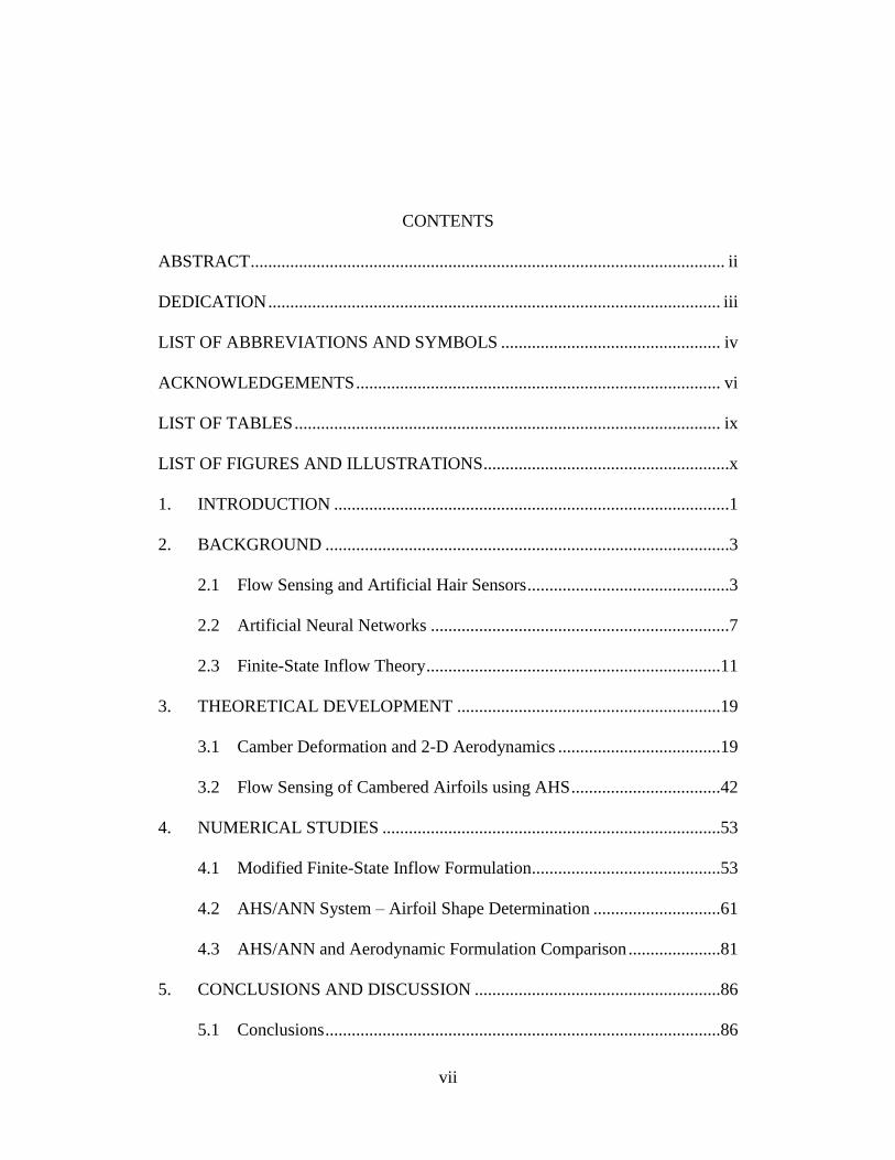
CONTENTS

ABSTRACT ............................................................................................................ ii

DEDICATION ....................................................................................................... iii

LIST OF ABBREVIATIONS AND SYMBOLS .................................................. iv

ACKNOWLEDGEMENTS ................................................................................... vi

LIST OF TABLES ................................................................................................. ix

LIST OF FIGURES AND ILLUSTRATIONS........................................................x

1. INTRODUCTION ..........................................................................................1

2. BACKGROUND ............................................................................................3

2.1 Flow Sensing and Artificial Hair Sensors ..............................................3

2.2 Artificial Neural Networks ....................................................................7

2.3 Finite-State Inflow Theory ...................................................................11

3. THEORETICAL DEVELOPMENT ............................................................19

3.1 Camber Deformation and 2-D Aerodynamics .....................................19

3.2 Flow Sensing of Cambered Airfoils using AHS ..................................42

4. NUMERICAL STUDIES .............................................................................53

4.1 Modified Finite-State Inflow Formulation ...........................................53

4.2 AHS/ANN System – Airfoil Shape Determination .............................61

4.3 AHS/ANN and Aerodynamic Formulation Comparison .....................81

5. CONCLUSIONS AND DISCUSSION ........................................................86

5.1 Conclusions ..........................................................................................86

viii

5.2 Contributions........................................................................................88

5.3 Future Work .........................................................................................89

REFERENCES ......................................................................................................90

ix

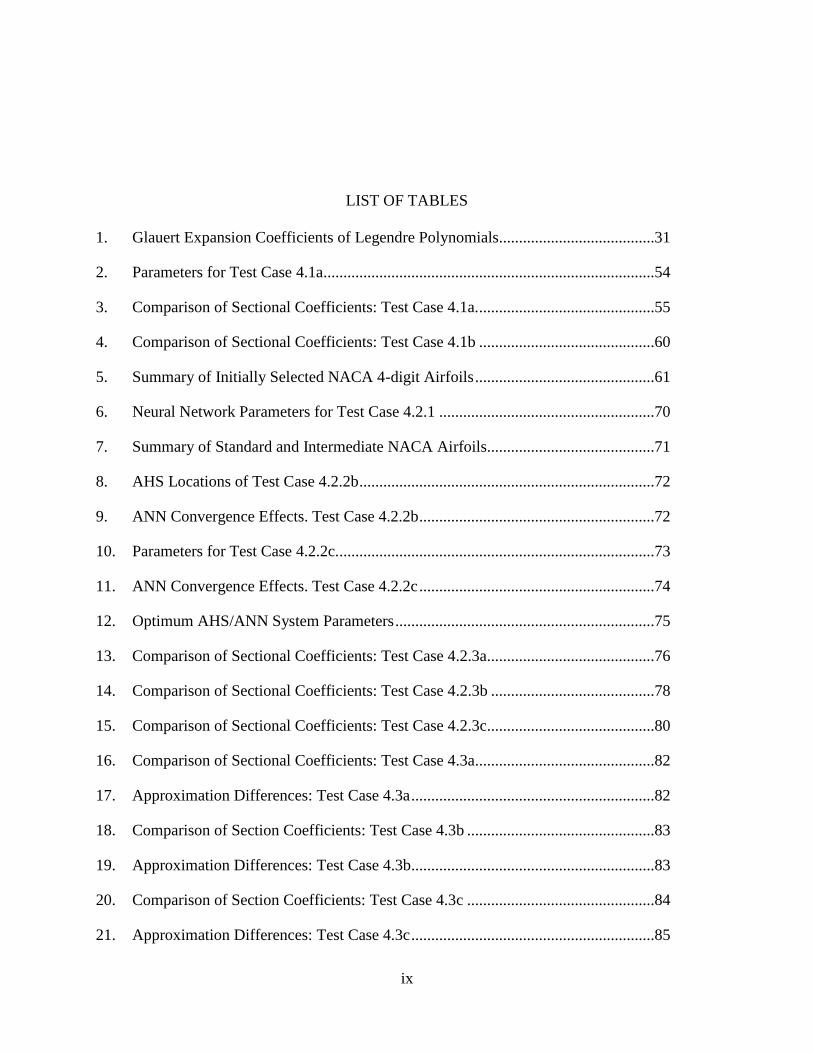
LIST OF TABLES

1. Glauert Expansion Coefficients of Legendre Polynomials.......................................31

2. Parameters for Test Case 4.1a ...................................................................................54

3. Comparison of Sectional Coefficients: Test Case 4.1a. ............................................55

4. Comparison of Sectional Coefficients: Test Case 4.1b ............................................60

5. Summary of Initially Selected NACA 4-digit Airfoils .............................................61

6. Neural Network Parameters for Test Case 4.2.1 ......................................................70

7. Summary of Standard and Intermediate NACA Airfoils..........................................71

8. AHS Locations of Test Case 4.2.2b ..........................................................................72

9. ANN Convergence Effects. Test Case 4.2.2b ...........................................................72

10. Parameters for Test Case 4.2.2c. ...............................................................................73

11. ANN Convergence Effects. Test Case 4.2.2c ...........................................................74

12. Optimum AHS/ANN System Parameters .................................................................75

13. Comparison of Sectional Coefficients: Test Case 4.2.3a ..........................................76

14. Comparison of Sectional Coefficients: Test Case 4.2.3b .........................................78

15. Comparison of Sectional Coefficients: Test Case 4.2.3c ..........................................80

16. Comparison of Sectional Coefficients: Test Case 4.3a .............................................82

17. Approximation Differences: Test Case 4.3a .............................................................82

18. Comparison of Section Coefficients: Test Case 4.3b ...............................................83

19. Approximation Differences: Test Case 4.3b.............................................................83

20. Comparison of Section Coefficients: Test Case 4.3c ...............................................84

21. Approximation Differences: Test Case 4.3c .............................................................85

x

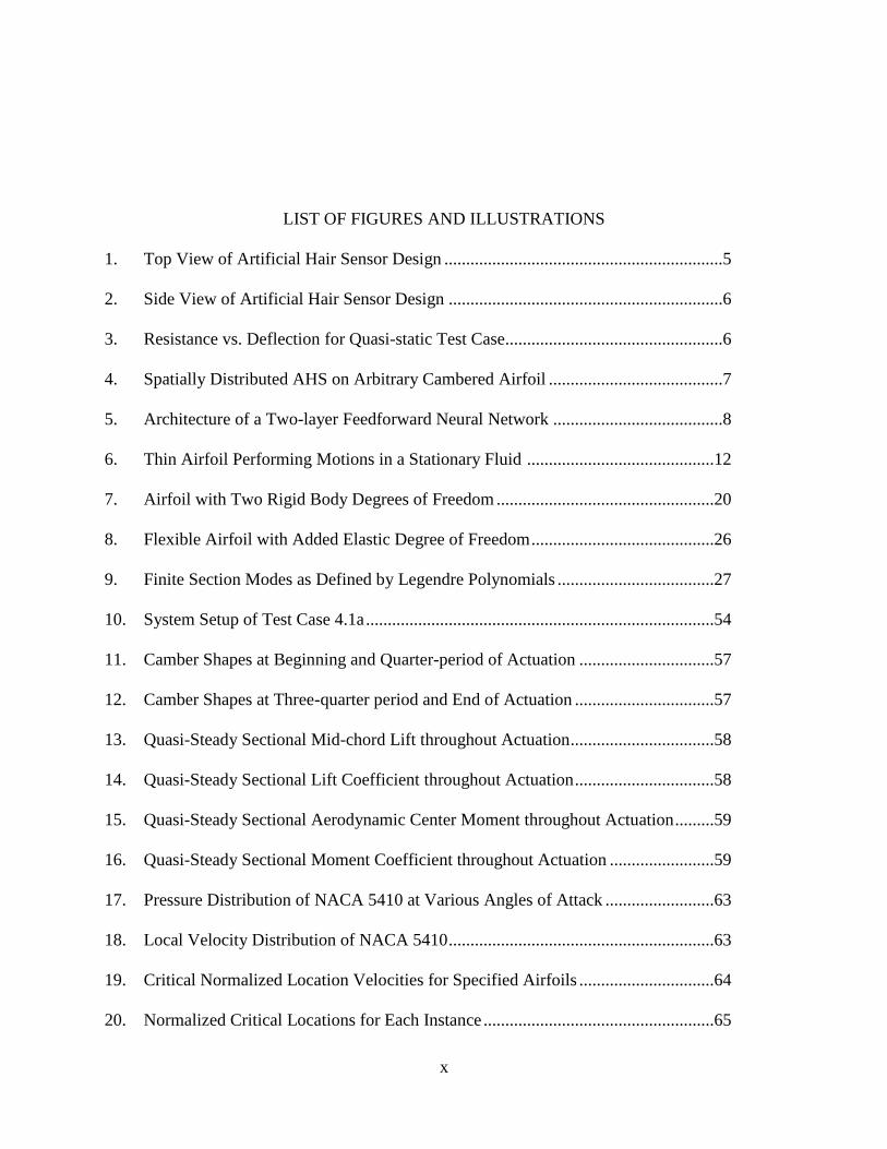
LIST OF FIGURES AND ILLUSTRATIONS

1. Top View of Artificial Hair Sensor Design ................................................................5

2. Side View of Artificial Hair Sensor Design ...............................................................6

3. Resistance vs. Deflection for Quasi-static Test Case ..................................................6

4. Spatially Distributed AHS on Arbitrary Cambered Airfoil ........................................7

5. Architecture of a Two-layer Feedforward Neural Network .......................................8

6. Thin Airfoil Performing Motions in a Stationary Fluid ...........................................12

7. Airfoil with Two Rigid Body Degrees of Freedom ..................................................20

8. Flexible Airfoil with Added Elastic Degree of Freedom ..........................................26

9. Finite Section Modes as Defined by Legendre Polynomials ....................................27

10. System Setup of Test Case 4.1a ................................................................................54

11. Camber Shapes at Beginning and Quarter-period of Actuation ...............................57

12. Camber Shapes at Three-quarter period and End of Actuation ................................57

13. Quasi-Steady Sectional Mid-chord Lift throughout Actuation .................................58

14. Quasi-Steady Sectional Lift Coefficient throughout Actuation ................................58

15. Quasi-Steady Sectional Aerodynamic Center Moment throughout Actuation .........59

16. Quasi-Steady Sectional Moment Coefficient throughout Actuation ........................59

17. Pressure Distribution of NACA 5410 at Various Angles of Attack .........................63

18. Local Velocity Distribution of NACA 5410 .............................................................63

19. Critical Normalized Location Velocities for Specified Airfoils ...............................64

20. Normalized Critical Locations for Each Instance .....................................................65

xi

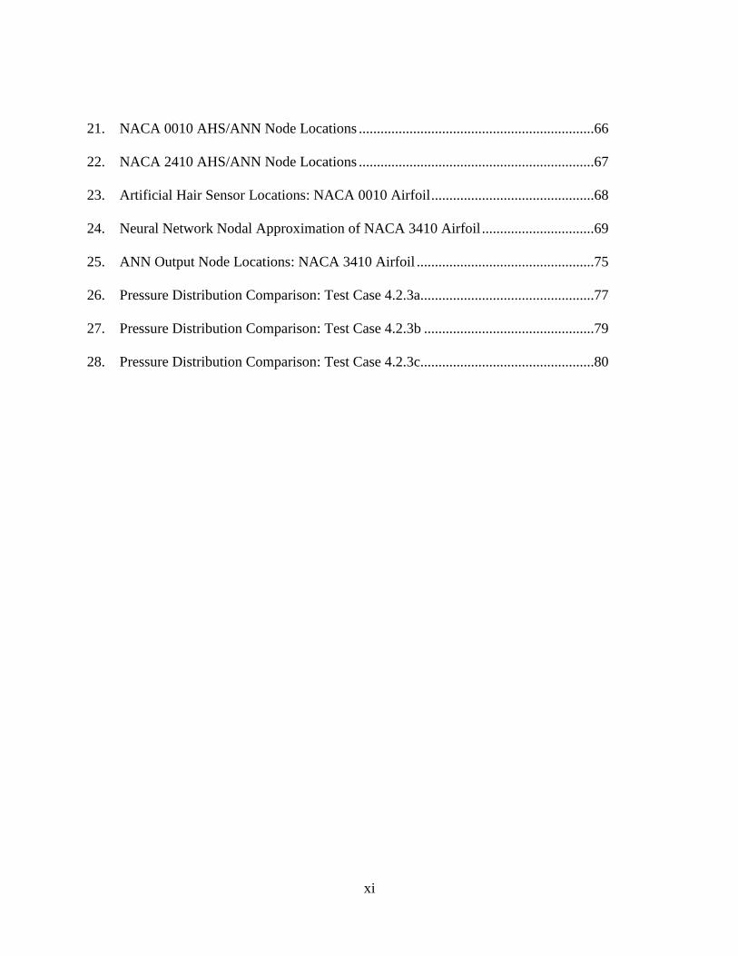
21. NACA 0010 AHS/ANN Node Locations .................................................................66

22. NACA 2410 AHS/ANN Node Locations .................................................................67

23. Artificial Hair Sensor Locations: NACA 0010 Airfoil .............................................68

24. Neural Network Nodal Approximation of NACA 3410 Airfoil ...............................69

25. ANN Output Node Locations: NACA 3410 Airfoil .................................................75

26. Pressure Distribution Comparison: Test Case 4.2.3a................................................77

27. Pressure Distribution Comparison: Test Case 4.2.3b ...............................................79

28. Pressure Distribution Comparison: Test Case 4.2.3c................................................80

1

CHAPTER 1

INTRODUCTION

In many recent morphing aircraft studies, airfoil and wing camber change have been

under investigation as important forms of shape control technology. Various camber-changing

methods have been used since the beginning of heavier-than-air flight, but camber change has

traditionally been introduced by using discrete leading- or trailing-edge flaps.1 Numerous

advantages can be gained by implementing camber variations along the chord-wise direction,

some of which are increased aerodynamic efficiency, reduced drag, and reduced wing-root

bending moments. Despite this, the concept of performing camber actuation on an airfoil that is

deformable along its entire chord length (fully deformable) has not been widely applied.2

Additionally, continuous camber-changing wings provide the ability to adaptively redistribute

wing loads, and thus can be used as a means of replacing conventional control surfaces,

ultimately leading to reduced structural weight. A fundamental problem of applying this concept

to real-world scenarios is the fact that camber actuation is a dynamic process. Thus, if camber

actuation is to be used as a means of control, there is a need to develop a theoretical formulation

to account for dynamic variations in the wing cross-sectional shape. Other studies (e.g., Ref. [3])

have utilized Computational Fluid Dynamics (CFD) to analyze the behaviors of airfoils with

dynamically changing cross-sections. A downside of using CFD is that it often requires high-

performance computing, and thus can be extremely time-consuming. Because of this, a more

efficient method based on the potential-flow theory (such as the finite-state inflow model that

2

was developed by Peters and his coworkers in [4]) may be used to provide a fast estimation of

the aerodynamic loads for airfoils with camber deformations. However, the formulation

developed in [4] only considers discrete flap deflection, and therefore must be expanded upon in

order for it to be used in preliminary design and analysis for the airloads on fully-deformable

airfoils.

In addition to preliminary analysis requirements, the dynamic nature of camber-changing

wings necessitates a means by which to obtain structural, aerodynamic, and flow states in real

time. In recent morphing technology research, the ability to sense, or “feel”, the current

aerodynamic and flow states in real time is achieved by implementing distributed flow sensors

and actuators on an aerial platform—a new concept referred to as Fly by Feel (FBF). One such

approach5 utilizes a new type of flow sensors, namely artificial hair sensors (AHS), which were

developed at the Air Force Research Laboratory (AFRL). Currently, AHS can be used to

determine the flow characteristics surrounding deformable airfoils. However, use of continuous

camber-changing wings also requires a method by which to obtain structural information (i.e.,

camber shape) in real-time, which has not yet been considered in previous flow sensing

applications. Therefore, the purpose of this thesis is to develop a two-dimensional, finite-state

aerodynamic formulation that is capable of accounting for arbitrary, dynamic camber

deformations, and a flow-sensing method utilizing AHS, similar to the one currently being used,

that also enables structural state awareness to be achieved in real time.

3

CHAPTER 2

BACKGROUND

2.1 Flow Sensing and Artificial Hair Sensors

Flow sensing is an essential technique in a wide range of applications, many of which

require sensitivity to low flow velocities.6 Such applications include traditional flow mapping,

turbulent flow characterization, self-stabilizing micro air vehicles (MAVs), and even biomedical

and biochemical applications. In addition to sensitivity at low flow velocities, these applications

require that the flow sensors also possess a short response time, low-detection threshold, and

minimal intrusion to the surrounding flow field.7

As is the case for much technical advancement, nature serves as a source of inspiration

and as a guide in the development of flow sensors for the aforementioned applications. Many

creatures live and maneuver in rapidly changing environments, and therefore are equipped with

flow-sensing mechanisms in order to survive in these complex changing environments. One such

example has been discovered on bats, which use tiny wing hairs to monitor flow conditions and

support flight control.8 Considering this, numerous flow sensor designs have been developed to

mimic those commonly found in nature.

The purpose of flow sensor utilization in this particular work is to enable fly-by-feel

(FBF), a concept in which distributed flow sensors and actuators are integrated on an aerial

platform to achieve aerodynamic state awareness and increase control. Artificial Hair Sensors

(AHS) are ideal flow sensors to use for FBF because they are lightweight, have low

4

manufacturing costs, and can be integrated on the surface of an aerial platform with minimal

flow disruption.5

In order to enable the FBF concept, AHS performs bio-like flow sensing by utilizing

insect-grade sensors to “feel” the air flow. When an AHS is subjected to a flow field, the glass

fiber hair undergoes a deflection. The magnitude of this deflection is proportional to the drag

force, FD , which is dependent upon the local flow velocity, v , and the geometry of the hair

surface.

(1)

(2)

Other parameters are defined as follows: ρ is the fluid density, CD is the drag coefficient, A is the

surface area normal to the flow, and D and L are the diameter and length of the carbon fiber hair,

respectively.

It should be noted that the root deflection is a function of the flow velocity and hair

stiffness, as shown in eqns. (1) and (2). Consequently, flow velocity limitations arise and must be

considered for each application. Subjecting an AHS to a flow velocity greater than the limiting

value will produce excessive deflection and cause erroneous measurements.

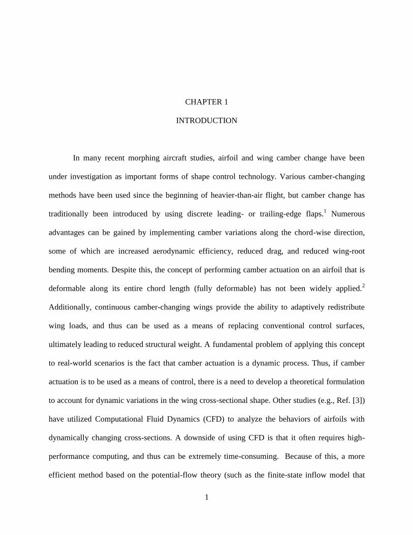
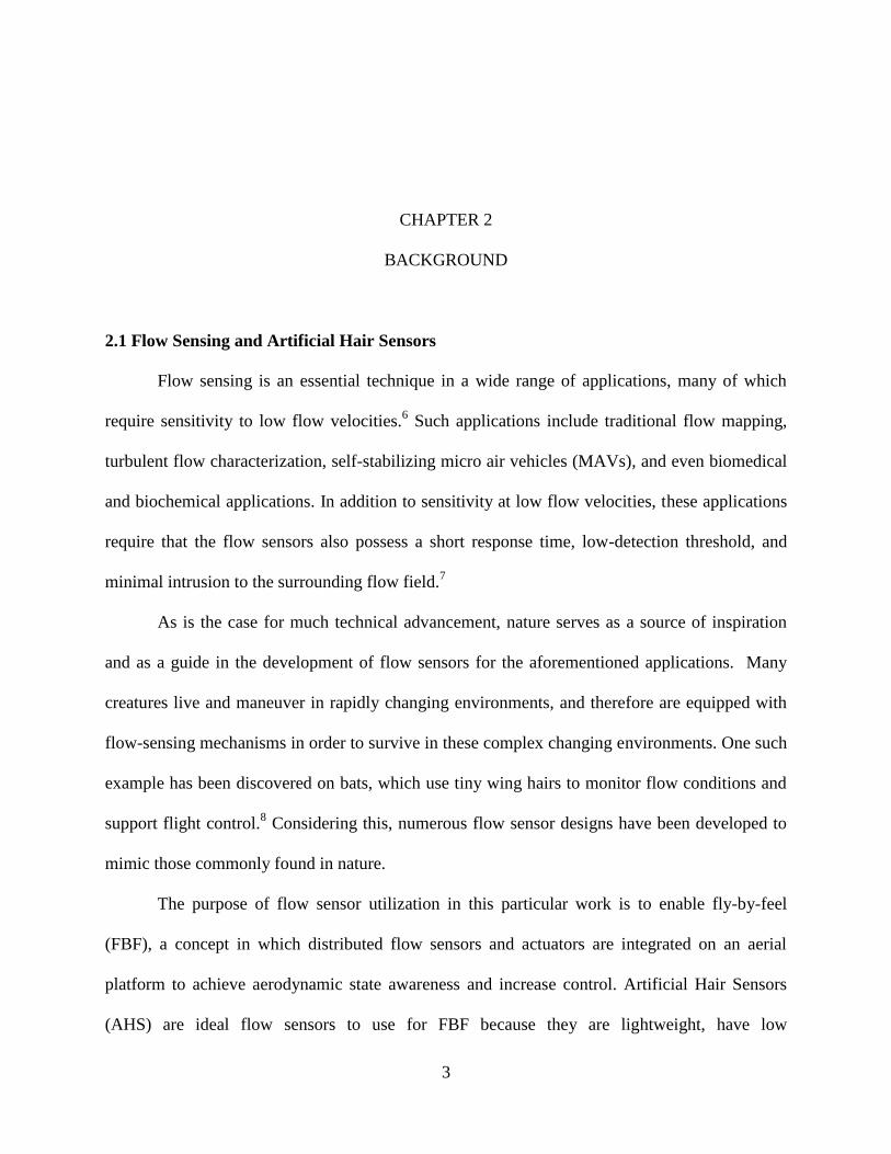
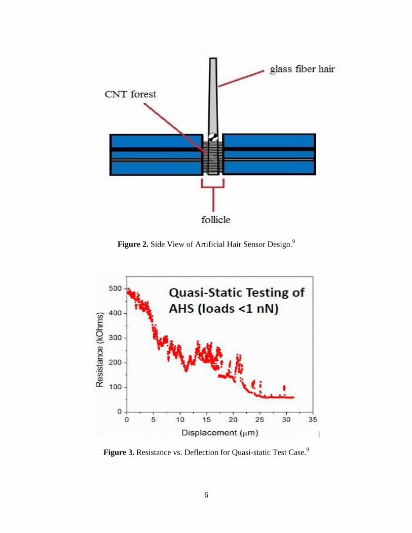
The AHS used in this application, as designed at the Air Force Research Laboratory

(AFRL), is comprised of three main components: a glass fiber hair, a carbon nano-tube (CNT)

“forest”, and a hair sensor “follicle”. This design is shown from a top view in Fig. 1, and from a

side view in Fig. 2. Although the exact length of the glass fiber hair can vary between individual

5

sensors, the AHS examined in this application typically extend approximately 2.5 mm above the

surface.

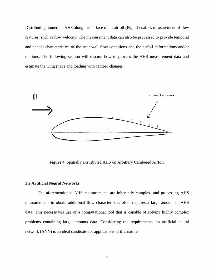
The CNT forest surrounds the base of the hair inside the follicle and is conductive in nature. The

CNT fibers contained in the forest are connected to electrodes, which are in turn connected to

electrical resistors. Deflection of the hair at the surface causes compression of the CNT fibers,

resulting in a resistance change that can be directly measured, as shown in Fig. 3.

Figure 1. Top View of Artificial Hair Sensor Design.

9

6

Figure 3. Resistance vs. Deflection for Quasi-static Test Case.9

Figure 2. Side View of Artificial Hair Sensor Design.9

7

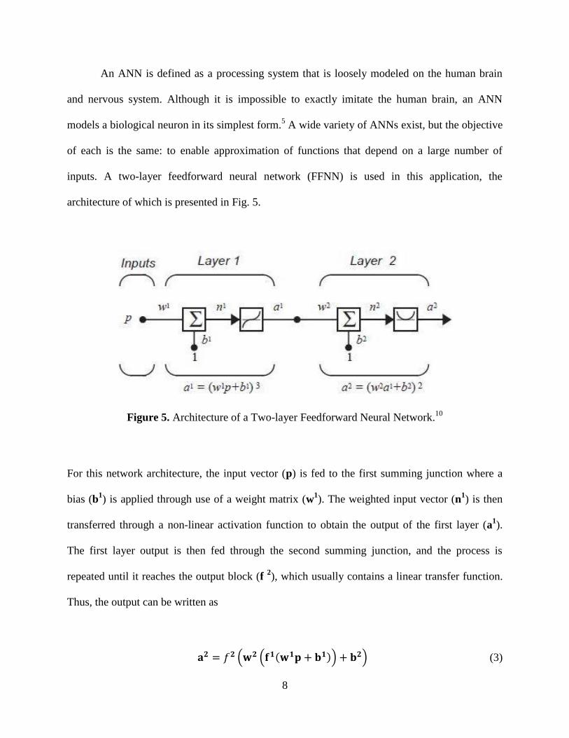
Distributing numerous AHS along the surface of an airfoil (Fig. 4) enables measurement of flow

features, such as flow velocity. The measurement data can also be processed to provide temporal

and spatial characteristics of the near-wall flow conditions and the airfoil deformations and/or

motions. The following section will discuss how to process the AHS measurement data and

estimate the wing shape and loading with camber changes.

2.2 Artificial Neural Networks

The aforementioned AHS measurements are inherently complex, and processing AHS

measurements to obtain additional flow characteristics often requires a large amount of AHS

data. This necessitates use of a computational tool that is capable of solving highly complex

problems containing large amounts data. Considering the requirements, an artificial neural

network (ANN) is an ideal candidate for applications of this nature.

Figure 4. Spatially Distributed AHS on Arbitrary Cambered Airfoil.

8

An ANN is defined as a processing system that is loosely modeled on the human brain

and nervous system. Although it is impossible to exactly imitate the human brain, an ANN

models a biological neuron in its simplest form.5 A wide variety of ANNs exist, but the objective

of each is the same: to enable approximation of functions that depend on a large number of

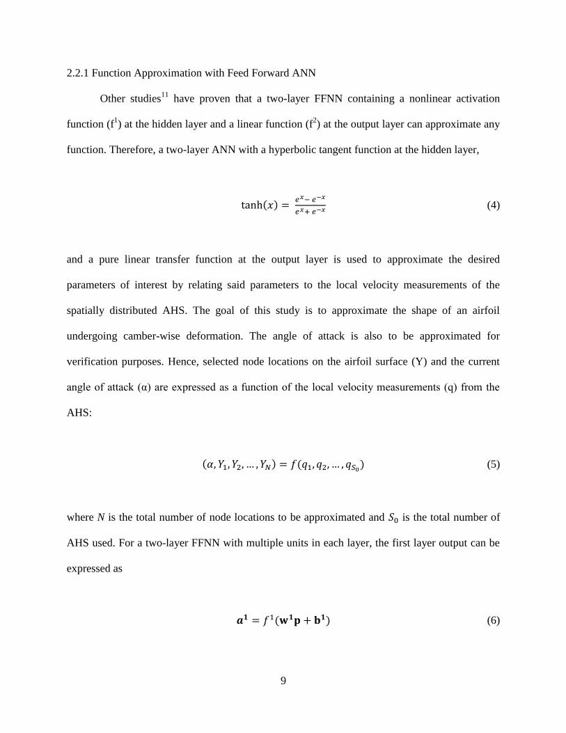
inputs. A two-layer feedforward neural network (FFNN) is used in this application, the

architecture of which is presented in Fig. 5.

For this network architecture, the input vector (p) is fed to the first summing junction where a

bias (b1) is applied through use of a weight matrix (w

1). The weighted input vector (n

1) is then

transferred through a non-linear activation function to obtain the output of the first layer (a1).

The first layer output is then fed through the second summing junction, and the process is

repeated until it reaches the output block (f 2), which usually contains a linear transfer function.

Thus, the output can be written as

(3)

Figure 5. Architecture of a Two-layer Feedforward Neural Network.10

9

2.2.1 Function Approximation with Feed Forward ANN

Other studies11

have proven that a two-layer FFNN containing a nonlinear activation

function (f1) at the hidden layer and a linear function (f

2) at the output layer can approximate any

function. Therefore, a two-layer ANN with a hyperbolic tangent function at the hidden layer,

(4)

and a pure linear transfer function at the output layer is used to approximate the desired

parameters of interest by relating said parameters to the local velocity measurements of the

spatially distributed AHS. The goal of this study is to approximate the shape of an airfoil

undergoing camber-wise deformation. The angle of attack is also to be approximated for

verification purposes. Hence, selected node locations on the airfoil surface (Y) and the current

angle of attack (α) are expressed as a function of the local velocity measurements (q) from the

AHS:

(5)

where N is the total number of node locations to be approximated and is the total number of

AHS used. For a two-layer FFNN with multiple units in each layer, the first layer output can be

expressed as

(6)

10

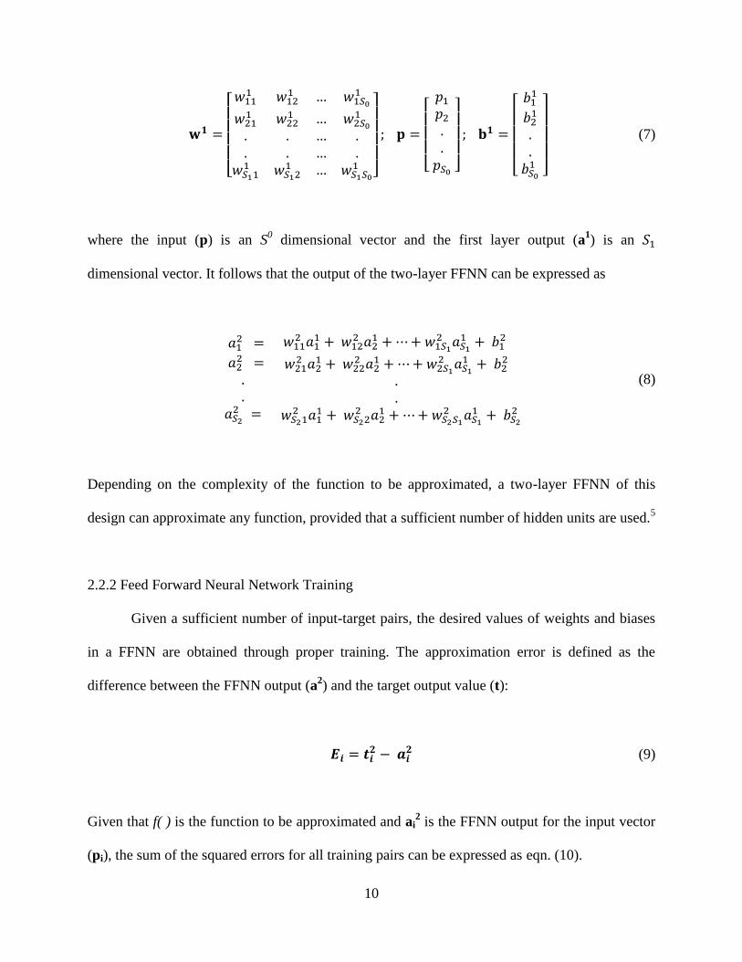
(7)

where the input (p) is an S0 dimensional vector and the first layer output (a

1) is an

dimensional vector. It follows that the output of the two-layer FFNN can be expressed as

(8)

Depending on the complexity of the function to be approximated, a two-layer FFNN of this

design can approximate any function, provided that a sufficient number of hidden units are used.5

2.2.2 Feed Forward Neural Network Training

Given a sufficient number of input-target pairs, the desired values of weights and biases

in a FFNN are obtained through proper training. The approximation error is defined as the

difference between the FFNN output (a2) and the target output value (t):

(9)

Given that f( ) is the function to be approximated and ai2 is the FFNN output for the input vector

(pi), the sum of the squared errors for all training pairs can be expressed as eqn. (10).

11

(10)

In order to accurately approximate the given input-target pair, eqn. (10) must be minimized. In

this study, optimization is done through use of a gradient-based algorithm, specifically the

Levenberg-Marquardt Back-propagation algorithm. Further information about this method can

be found in Ref. [5].

2.3 Finite-State Inflow Theory

In a precise sense, 2-D unsteady aerodynamics is an infinite state process, and therefore

has no finite-state representation. However, there are numerous advantages of finite state models.

First, finite state modeling allows one to cast the aerodynamics in the same state-space context as

the structural dynamics and controls. Second, the existence of explicit states negates the need to

iterate on solutions. Instead, the solution can be obtained in a single pass. Additionally, the

flexibility of a finite state model allows for it to be exercised in the frequency domain, Laplace

domain, or the time domain as desired.12

Recent trends in rotor control theory have emphasized the potential benefits of individual

blade control for vibration alleviation, handling improvements, and increased stability. Similarly,

the application of this concept has been extended to include servo-flaps and smart structures.

With this in mind, a general finite state theory of deformable airfoils was developed as presented

in Ref. [4]. An overview of this theory is given in the following section.

12

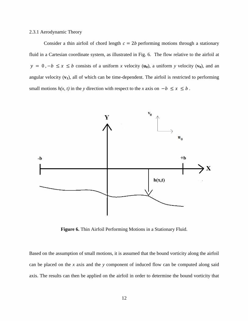
2.3.1 Aerodynamic Theory

Consider a thin airfoil of chord length performing motions through a stationary

fluid in a Cartesian coordinate system, as illustrated in Fig. 6. The flow relative to the airfoil at

consists of a uniform x velocity (u0), a uniform y velocity (v0), and an

angular velocity (v1), all of which can be time-dependent. The airfoil is restricted to performing

small motions h(x, t) in the y direction with respect to the x axis on .

Based on the assumption of small motions, it is assumed that the bound vorticity along the airfoil

can be placed on the x axis and the y component of induced flow can be computed along said

axis. The results can then be applied on the airfoil in order to determine the bound vorticity that

Figure 6. Thin Airfoil Performing Motions in a Stationary Fluid.

13

will enforce the non-penetration boundary condition on the moving airfoil. The necessary

induced flow in the negative y direction due to bound vorticity can then be written as4

(11)

where λ is the downwash due to all other free vorticity. The relationship between and the

unknown bound vorticity ( ) is then given as4

(12)

Thus, eqns. (11) and (12) combine to form the non-penetration boundary condition. The pressure

difference across the airfoil can then be found from the pressure-vorticity equation.

(13)

Equations (11) – (13) form the complete theory of air loads for a deformable airfoil. They are

then combined with an induced-flow model for λ in order to close the system. In accordance with

Ref. [4], this is accomplished by enforcing eqns. (14) and (15).

(14)

14

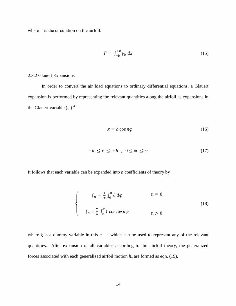
where Γ is the circulation on the airfoil:

(15)

2.3.2 Glauert Expansions

In order to convert the air load equations to ordinary differential equations, a Glauert

expansion is performed by representing the relevant quantities along the airfoil as expansions in

the Glauert variable (φ).4

(16)

(17)

It follows that each variable can be expanded into n coefficients of theory by

(18)

where ξ is a dummy variable in this case, which can be used to represent any of the relevant

quantities. After expansion of all variables according to thin airfoil theory, the generalized

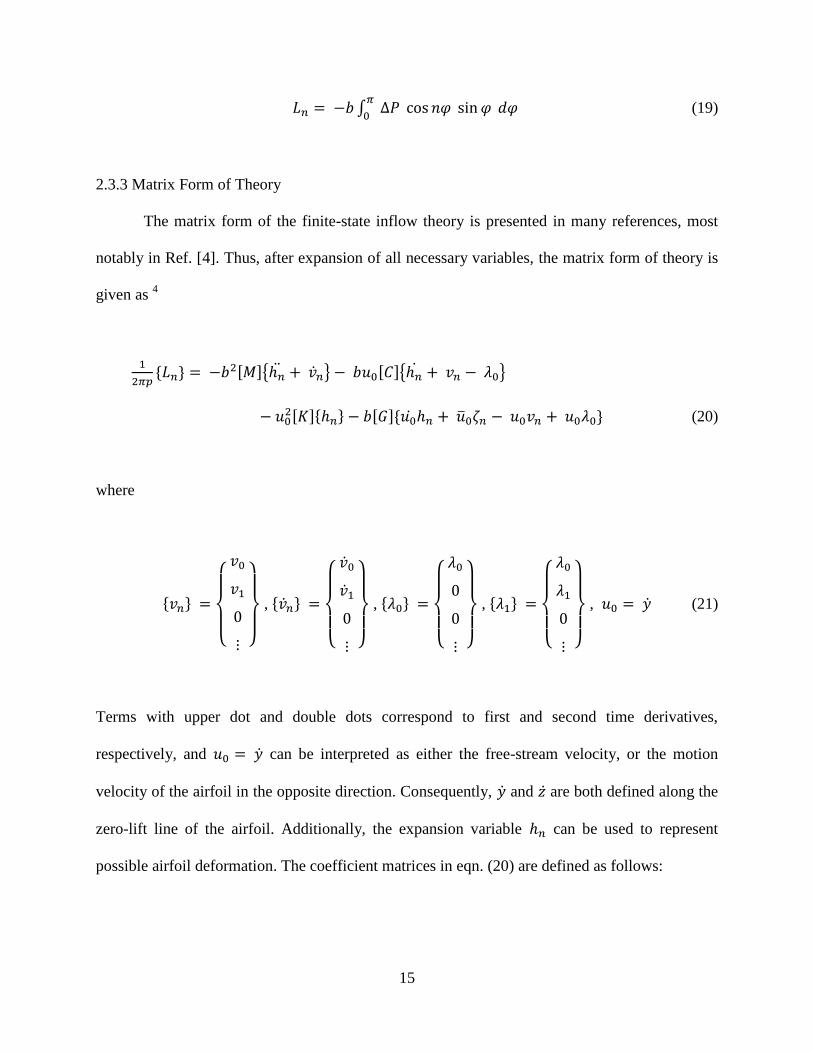
forces associated with each generalized airfoil motion hn are formed as eqn. (19).

15

(19)

2.3.3 Matrix Form of Theory

The matrix form of the finite-state inflow theory is presented in many references, most

notably in Ref. [4]. Thus, after expansion of all necessary variables, the matrix form of theory is

given as 4

(20)

where

,

,

,

, (21)

Terms with upper dot and double dots correspond to first and second time derivatives,

respectively, and can be interpreted as either the free-stream velocity, or the motion

velocity of the airfoil in the opposite direction. Consequently, and are both defined along the

zero-lift line of the airfoil. Additionally, the expansion variable can be used to represent

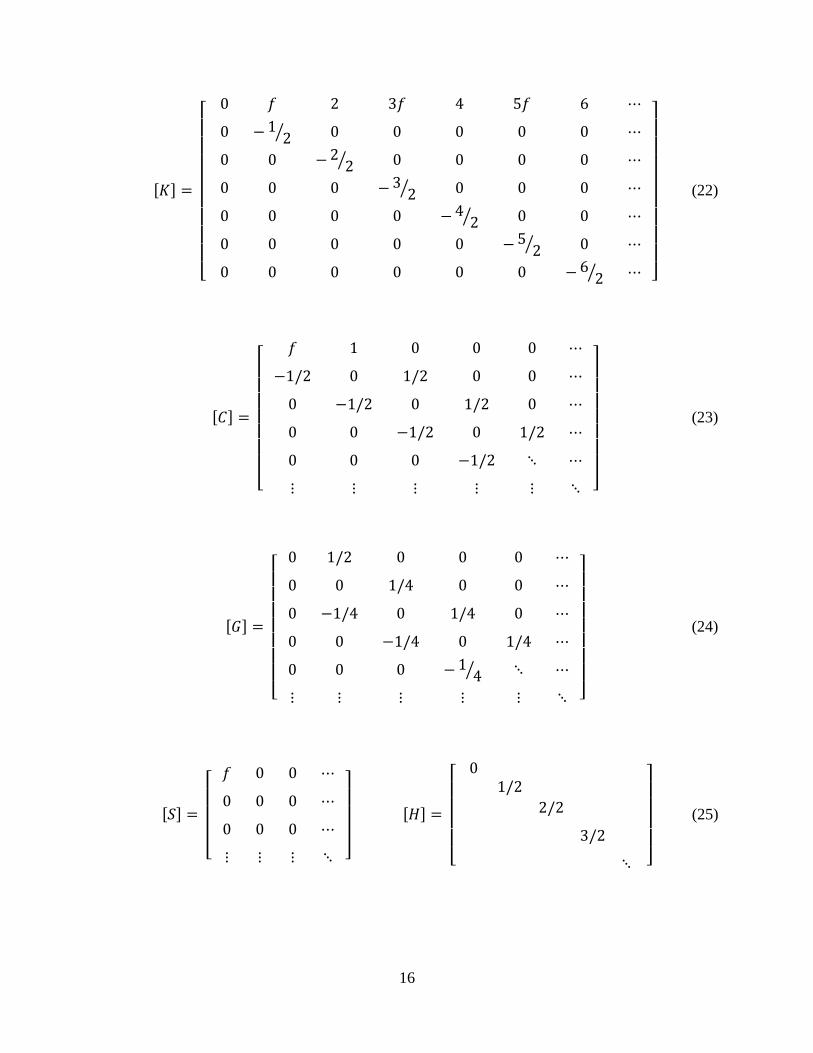
possible airfoil deformation. The coefficient matrices in eqn. (20) are defined as follows:

16

(22)

(23)

(24)

(25)

17

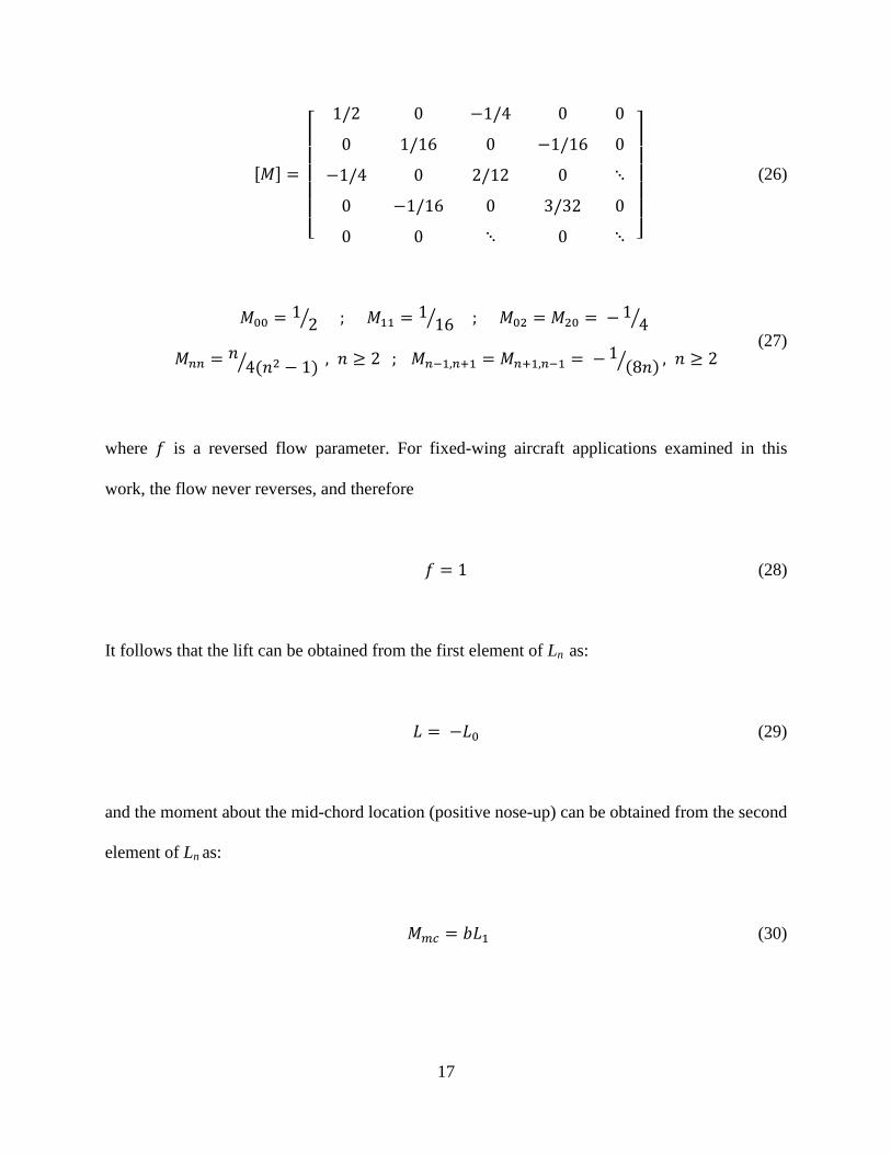
(26)

(27)

where is a reversed flow parameter. For fixed-wing aircraft applications examined in this

work, the flow never reverses, and therefore

(28)

It follows that the lift can be obtained from the first element of Ln as:

(29)

and the moment about the mid-chord location (positive nose-up) can be obtained from the second

element of Ln as:

(30)

18

Also, assuming pressure loads are applied along the airfoil camber line, the generalized camber

force per unit span is given as:

(31)

The drag calculated from the potential flow theory is essentially the lift component acting along

the direction of the free stream velocity, 13

and is therefore obtained as:

(32)

19

CHAPTER 3

THEORETICAL DEVELOPMENT

3.1 Camber Deformation and 2-D Aerodynamics

In order to develop a two-dimensional aerodynamic formulation according to the defined

requirements, previous applications of two-dimensional finite-state formulations need be first

examined. Once the groundwork is outlined, the previous developments can be expanded upon to

meet the requirements of this work.

3.1.1 Finite-State Inflow Theory: Rigid Airfoil

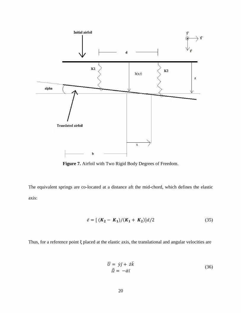
The first system subject to study14

is illustrated in Fig. 7. A thin airfoil, initially located

along the x axis and spanning from –b to b, is subjected to a uniform free-stream velocity ( ).

Initially, only two degrees of freedom (dof) are considered: plunge (z), pitch (α). The airfoil is

attached to two linear springs of stiffness K1 and K2, each of which is located at a distance d/2

from the mid-chord. This combination of springs is equivalent to a translational spring and a

torsional spring with individual stiffness coefficients given by eqns. (33) and (34), respectively.

(33)

(34)

20

The equivalent springs are co-located at a distance aft the mid-chord, which defines the elastic

axis:

(35)

Thus, for a reference point ξ placed at the elastic axis, the translational and angular velocities are

(36)

Figure 7. Airfoil with Two Rigid Body Degrees of Freedom.

21

and the translational acceleration is

(37)

where and are the plunging and pitching (angular) velocity of the reference point,

respectively. For an arbitrary point along the airfoil, the velocity is

(38)

and the acceleration is

(39)

Thus, at any point on the airfoil, the flow’s downward velocity is given as (positive down):

(40)

and the vertical acceleration is given as:

(41)

22

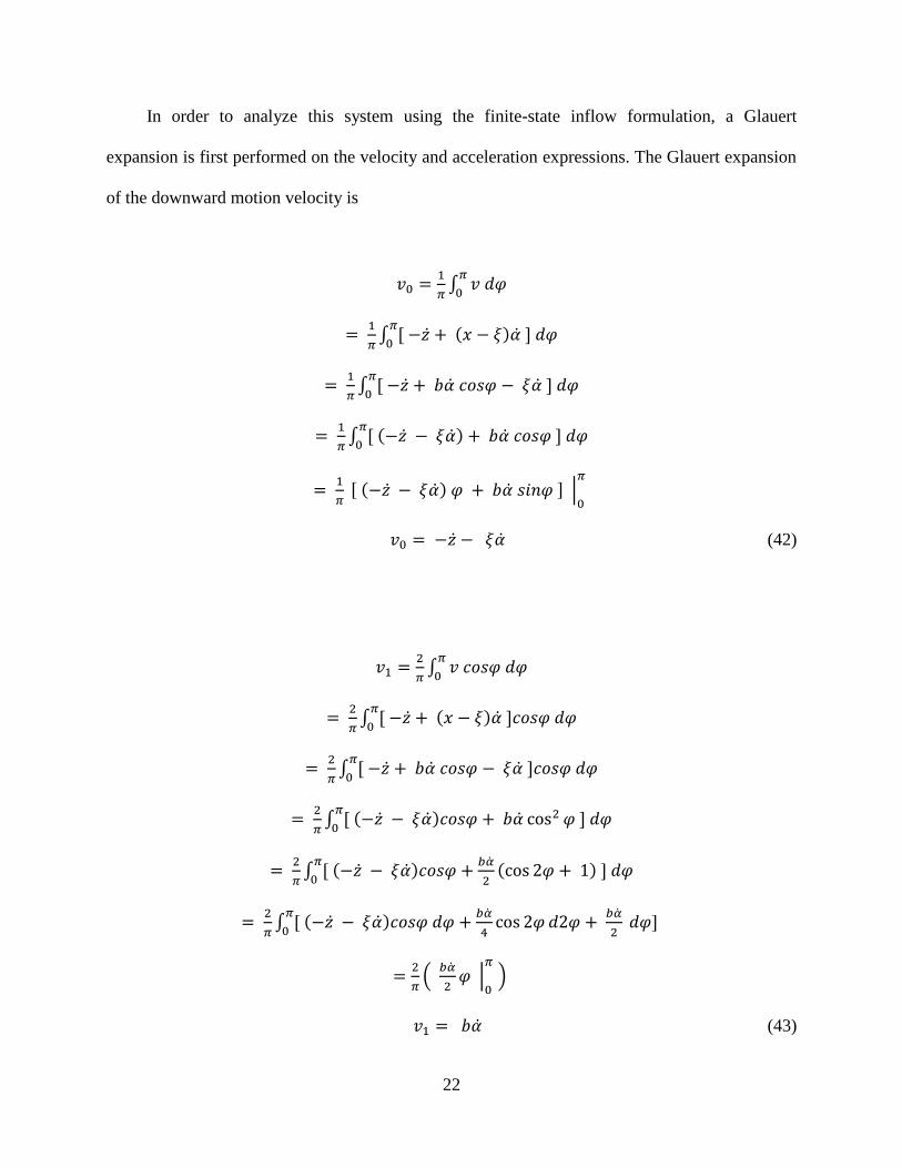
In order to analyze this system using the finite-state inflow formulation, a Glauert

expansion is first performed on the velocity and acceleration expressions. The Glauert expansion

of the downward motion velocity is

(42)

(43)

23

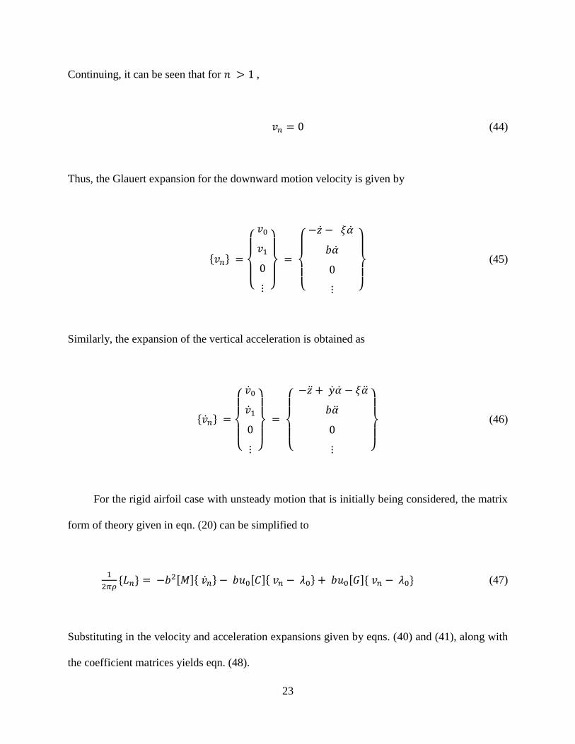
Continuing, it can be seen that for ,

(44)

Thus, the Glauert expansion for the downward motion velocity is given by

(45)

Similarly, the expansion of the vertical acceleration is obtained as

(46)

For the rigid airfoil case with unsteady motion that is initially being considered, the matrix

form of theory given in eqn. (20) can be simplified to

(47)

Substituting in the velocity and acceleration expansions given by eqns. (40) and (41), along with

the coefficient matrices yields eqn. (48).

24

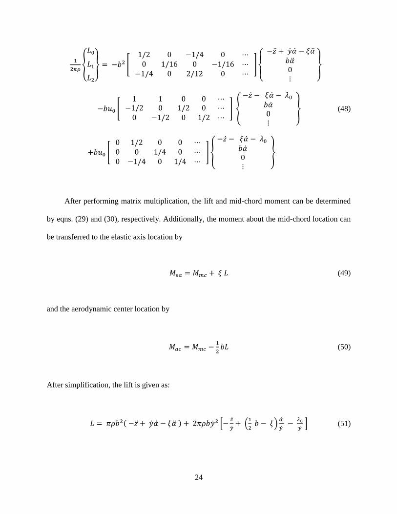
(48)

After performing matrix multiplication, the lift and mid-chord moment can be determined

by eqns. (29) and (30), respectively. Additionally, the moment about the mid-chord location can

be transferred to the elastic axis location by

(49)

and the aerodynamic center location by

(50)

After simplification, the lift is given as:

(51)

25

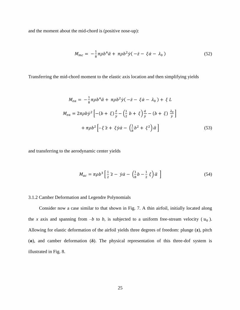
and the moment about the mid-chord is (positive nose-up):

(52)

Transferring the mid-chord moment to the elastic axis location and then simplifying yields

–

(53)

and transferring to the aerodynamic center yields

(54)

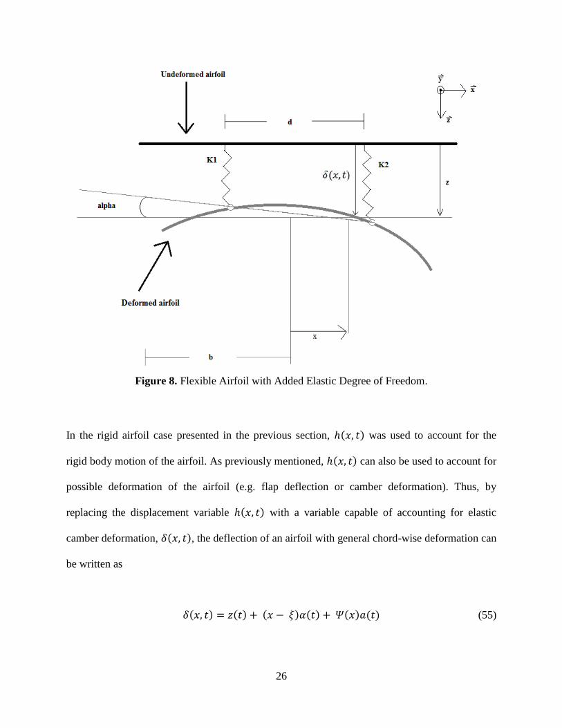
3.1.2 Camber Deformation and Legendre Polynomials

Consider now a case similar to that shown in Fig. 7. A thin airfoil, initially located along

the x axis and spanning from –b to b, is subjected to a uniform free-stream velocity ( ).

Allowing for elastic deformation of the airfoil yields three degrees of freedom: plunge (z), pitch

(α), and camber deformation (δ). The physical representation of this three-dof system is

illustrated in Fig. 8.

26

In the rigid airfoil case presented in the previous section, was used to account for the

rigid body motion of the airfoil. As previously mentioned, can also be used to account for

possible deformation of the airfoil (e.g. flap deflection or camber deformation). Thus, by

replacing the displacement variable with a variable capable of accounting for elastic

camber deformation, , the deflection of an airfoil with general chord-wise deformation can

be written as

(55)

Figure 8. Flexible Airfoil with Added Elastic Degree of Freedom.

27

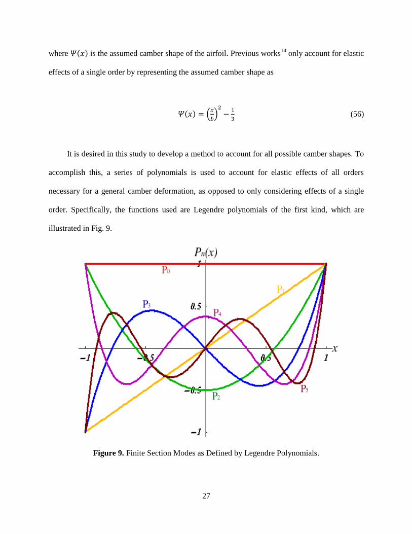
where is the assumed camber shape of the airfoil. Previous works14

only account for elastic

effects of a single order by representing the assumed camber shape as

(56)

It is desired in this study to develop a method to account for all possible camber shapes. To

accomplish this, a series of polynomials is used to account for elastic effects of all orders

necessary for a general camber deformation, as opposed to only considering effects of a single

order. Specifically, the functions used are Legendre polynomials of the first kind, which are


Figure 9. Finite Section Modes as Defined by Legendre Polynomials.

28

Legendre polynomials are continuous by definition and defined within the domain

. These polynomials were chosen to represent arbitrary camber deformations because they

naturally resemble mode shapes frequently seen in free-free beam bending deflections. For

example, represents an un-deformed beam, represents rigid-body motions (plunge and

pitch), and represents a free-free beam deflection. It follows that can be expressed in

terms of a coordinate along the chord-wise direction (ξ which is defined in terms of the

Glauert variable φ such that

(57)

Therefore, the set of Legendre polynomials is given as:

(58)

Referring to eqn. (55), it can be seen that the third term on the right hand side represents the

elastic camber deformation of the airfoil. Defining the elastic camber deformation as such yields

29

(59)

where

(60)

Thus, the Legendre polynomials of eqn. (58) can be used to represent the assumed camber shape,

Ψ(x). It follows that the elastic camber deformation is determined by Glauert expansion of the

finite section mode(s) and the corresponding magnitude(s).

a) Single mode approximation

A single mode approximation using the finite state mode is given as:

(61)

The Glauert expansion of is derived as:

φ φ φ

(62)

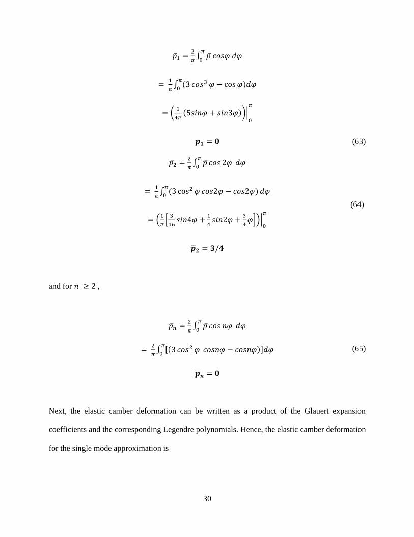
30

(63)

(64)

and for ,

(65)

Next, the elastic camber deformation can be written as a product of the Glauert expansion

coefficients and the corresponding Legendre polynomials. Hence, the elastic camber deformation

for the single mode approximation is

31

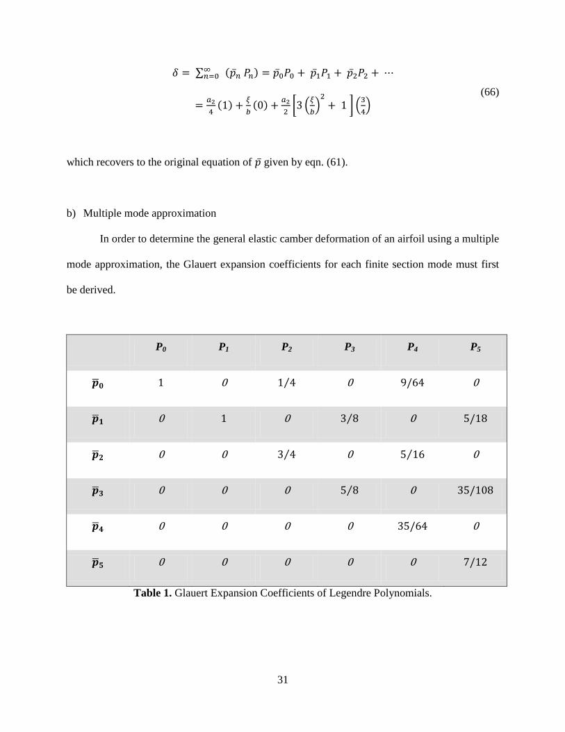
(66)

which recovers to the original equation of given by eqn. (61).

b) Multiple mode approximation

In order to determine the general elastic camber deformation of an airfoil using a multiple

mode approximation, the Glauert expansion coefficients for each finite section mode must first

be derived.

P0 P1 P2 P3 P4 P5

1 0 0 0

0 0 0

0 0 0 0

0 0 0 0

0 0 0 0 0

0 0 0 0 0

Table 1. Glauert Expansion Coefficients of Legendre Polynomials.

32

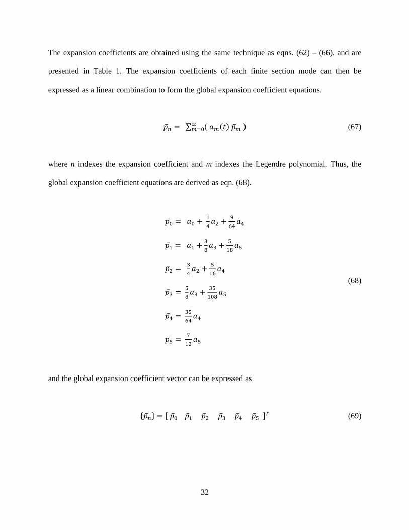
The expansion coefficients are obtained using the same technique as eqns. (62) – (66), and are

presented in Table 1. The expansion coefficients of each finite section mode can then be

expressed as a linear combination to form the global expansion coefficient equations.

(67)

where n indexes the expansion coefficient and m indexes the Legendre polynomial. Thus, the

global expansion coefficient equations are derived as eqn. (68).

(68)

and the global expansion coefficient vector can be expressed as

(69)

33

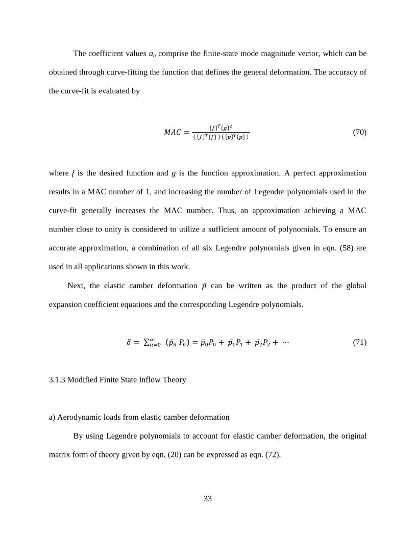
The coefficient values an comprise the finite-state mode magnitude vector, which can be

obtained through curve-fitting the function that defines the general deformation. The accuracy of

the curve-fit is evaluated by

(70)

where f is the desired function and g is the function approximation. A perfect approximation

results in a MAC number of 1, and increasing the number of Legendre polynomials used in the

curve-fit generally increases the MAC number. Thus, an approximation achieving a MAC

number close to unity is considered to utilize a sufficient amount of polynomials. To ensure an

accurate approximation, a combination of all six Legendre polynomials given in eqn. (58) are

used in all applications shown in this work.

Next, the elastic camber deformation can be written as the product of the global

expansion coefficient equations and the corresponding Legendre polynomials.

(71)

3.1.3 Modified Finite State Inflow Theory

a) Aerodynamic loads from elastic camber deformation

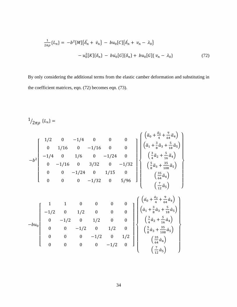
By using Legendre polynomials to account for elastic camber deformation, the original

matrix form of theory given by eqn. (20) can be expressed as eqn. (72).

34

(72)

By only considering the additional terms from the elastic camber deformation and substituting in

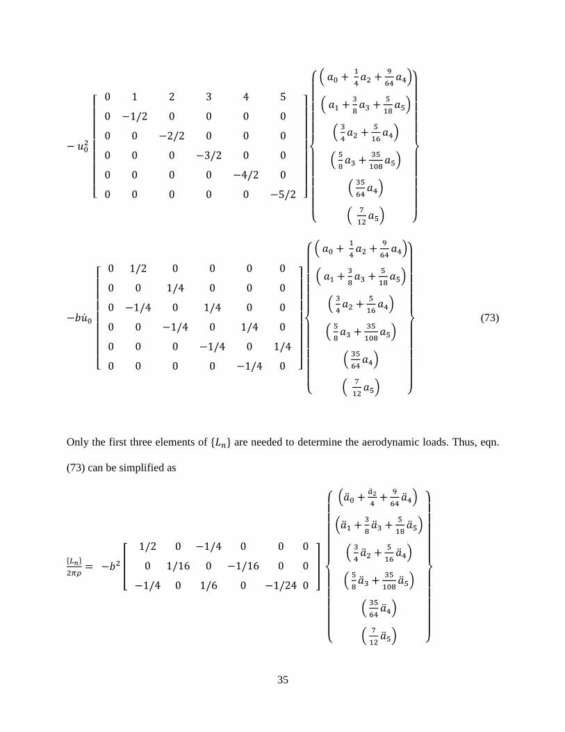
the coefficient matrices, eqn. (72) becomes eqn. (73).

35

(73)

Only the first three elements of are needed to determine the aerodynamic loads. Thus, eqn.

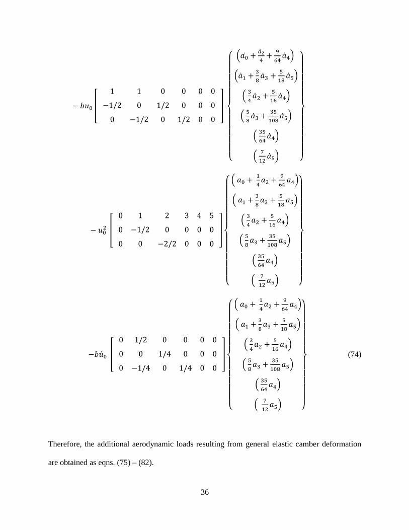
(73) can be simplified as

36

(74)

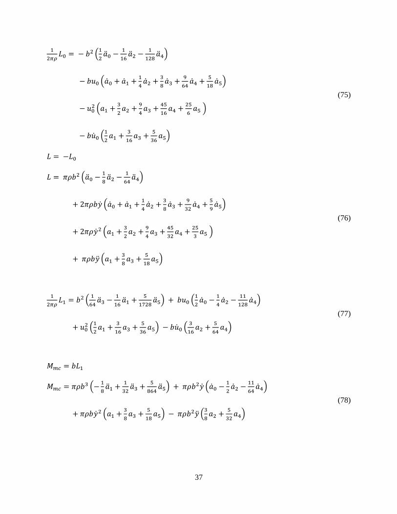
Therefore, the additional aerodynamic loads resulting from general elastic camber deformation

are obtained as eqns. (75) – (82).

37

(75)

(76)

(77)

(78)

38

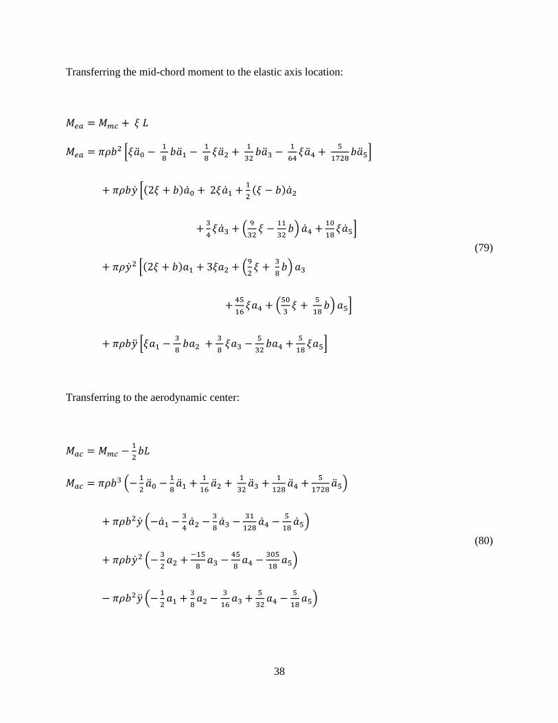
Transferring the mid-chord moment to the elastic axis location:

(79)

Transferring to the aerodynamic center:

(80)

39

Also, the generalized camber force per unit span is obtained as:

(81)

(82)

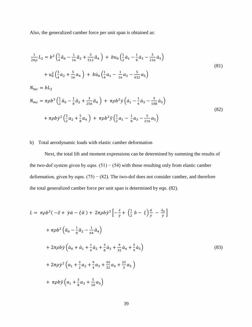
b) Total aerodynamic loads with elastic camber deformation

Next, the total lift and moment expressions can be determined by summing the results of

the two-dof system given by eqns. (51) − (54) with those resulting only from elastic camber

deformation, given by eqns. (75) − (82). The two-dof does not consider camber, and therefore

the total generalized camber force per unit span is determined by eqn. (82).

(83)

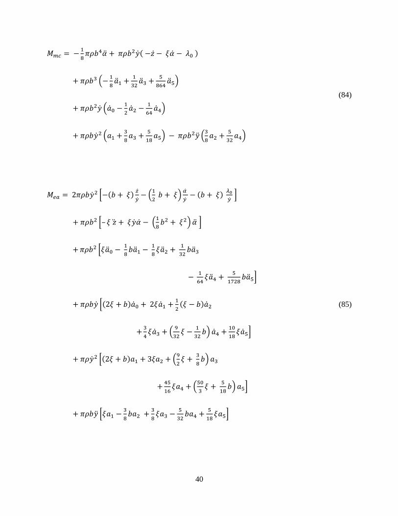
40

(84)

–

(85)

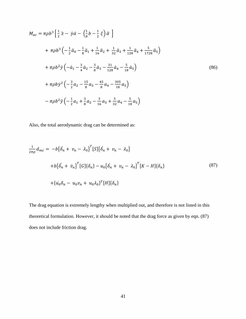
41

(86)

Also, the total aerodynamic drag can be determined as:

(87)

The drag equation is extremely lengthy when multiplied out, and therefore is not listed in this

theoretical formulation. However, it should be noted that the drag force as given by eqn. (87)

does not include friction drag.

42

3.2 Flow Sensing of Cambered Airfoils Using AHS

3.2.1 Airfoil Selection

In an ideal scenario, the AHS/ANN approximation would be carried out for a thin airfoil

shape so that the aerodynamic results could be directly compared to those from the previously

developed aerodynamic formulation for camber-wise deformation. However, XFoil is only

capable of performing subsonic analysis for airfoils of finite thickness; therefore, this direct

approach is not possible. Since XFoil allows for input of NACA 4 and 5-digit airfoil shapes, it

was decided that a variety of NACA 4-digit airfoil shapes would be used to simulate camber-

wise deformation.

For review, the first number of the NACA 4-digit series defines the maximum camber as

a percent of the chord length. The second digit defines the location of the maximum camber

along the chord-line as tens of percent of the chord length. The last two digits define the

maximum thickness of the airfoil as a percent of the chord. Using this approach, camber-wise

deformation can be applied by changing the first and/or second digit of a NACA 4-digit airfoil.

Although the first digit of NACA 4-digit series airfoils can theoretically be varied from 0-9,

common practices in airfoil design typically use values ranging from 0-5. Maximum camber

values above this range result in increased drag forces that often outweigh advantages of the

additional lift produced by high camber.

In addition, the limitations of the ANN must be considered when defining the airfoils to

be used. As previously discussed, the size of the ANN training data directly affects

computational requirements. A high variance of airfoil shapes in the data set must be countered

by a decreased number of data intervals in order to limit the overall size of the data set. Doing so

43

reduces mesh refinement, which ultimately results in higher approximation error. Also, since

camber actuation is a continuous process, there can be many times throughout the actuation

process where the airfoil shape is not a defined NACA 4-digit airfoil, but rather some

intermediate shape between defined 4-digit shapes. Therefore, it is desirable to include

intermediate NACA 4-digit airfoil shapes in the training data in order to increase mesh

refinement and approximation accuracy.

3.2.2 AHS Limitations and Flow Parameters

Other important factors that must be considered are the properties and limitations of the

AHS. The AHS currently being used can only perform effectively at flow velocity values below

the limiting value, . Subjecting an AHS to a flow velocity greater than this limiting

value produces excessive bending in the AHS, resulting in erroneous data. It is also important to

keep in mind that this limiting velocity refers to the velocity experienced by each sensor, not the

free-stream velocity. Basic aerodynamic principles show that subjecting an airfoil to a free-

stream flow can result in some areas of the airfoil surface experiencing local velocity values

higher than that of the free-stream. Thus, the normalized local velocity limit is given by eqn.

(88).

(88)

These areas of higher local velocity can vary depending on airfoil shape and angle of attack.

Other phenomena that may occur in critical areas along the airfoil surface, such as stagnation

44

near the leading and trailing edges, can also have a drastic effect on the accuracy of the AHS

readings and must be taken into consideration.

3.2.3 Critical Regions

The aforementioned phenomena that occur in the critical regions of an airfoil surface can

cause inaccuracies in AHS readings, and therefore must be considered when determining

AHS/ANN node locations. These AHS/ANN nodes can be used as ANN inputs (local velocities),

ANN outputs (node location approximations), or both. When a node location is defined as an

ANN input, it is effectively simulating the placement of an AHS at that node location. Thus,

further analysis of the critical regions must be performed in order to characterize the flow

conditions and node locations for which the AHS can effectively perform. These critical regions

are most easily determined by examining the local velocity distributions along the airfoil surface

at varying free-stream velocities and angles of attack. Additionally, the local pressure

coefficients are considered to verify the accuracy of the local velocity values. This is done

through a combination of the pressure coefficient definition and Bernoulli’s equation, as shown

in eqn. (89).

(89)

Numerous aerodynamic studies have shown that the highest maximum local velocity

values correspond to the most drastic values of . Therefore, by holding the free-stream velocity

constant at the maximum design value and considering at both limiting angles of attack (

and , XFoil analysis is performed for each desired airfoil shape in order to locate critical

45

regions in which this local velocity limit may be exceeded. These critical local velocity values

generally occur near the leading edge. Since XFoil is used for flow analysis in this work, it

should be noted that some critical local velocity values are likely the result of shortcomings in

the XFoil analysis near the stagnation points. However, critical local velocity values that occur at

a greater distance from the leading edge are proven accurate and should be expected in real-

world applications. Therefore, it is necessary to define the critical regions of all airfoil shapes

and flow conditions with more accuracy.

To accomplish this, the critical normalized local velocity values and their corresponding

locations are analyzed for each individual instance (airfoil shape and angle of attack). To

determine the domain of the critical region for each individual airfoil, the location of greatest

distance from the leading edge at which is defined as the relevant value. The

critical location for each airfoil, , is then be normalized with the chord length and plotted

versus the corresponding critical normalized local velocity value. The maximum critical location

of the airfoil shapes and flow conditions being considered is then used to define the leading edge

critical region, as shown in eqn. (90). All locations within this critical region must be eliminated

when considering the AHS/ANN node locations.

(90)

Although critical local velocities generally do not occur near the trailing edge, flow stagnation as

a result of the Kutta condition can lead to inaccuracies if AHS are placed in this region.

Additionally, flow stagnation at the trailing edge can lead to computational difficulties during

XFoil analysis. To avoid these difficulties, default NACA airfoils in XFoil contain a small gap

46

between the upper and lower airfoil surfaces at the trailing edge. Although this effectively

prevents flow stagnation at the trailing edge point, local velocities slightly trend towards

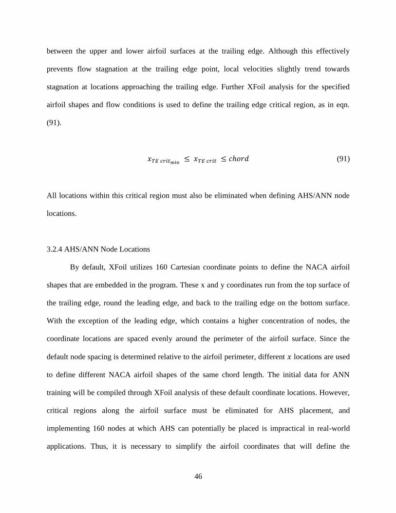
stagnation at locations approaching the trailing edge. Further XFoil analysis for the specified

airfoil shapes and flow conditions is used to define the trailing edge critical region, as in eqn.

(91).

(91)

All locations within this critical region must also be eliminated when defining AHS/ANN node

locations.

3.2.4 AHS/ANN Node Locations

By default, XFoil utilizes 160 Cartesian coordinate points to define the NACA airfoil

shapes that are embedded in the program. These x and y coordinates run from the top surface of

the trailing edge, round the leading edge, and back to the trailing edge on the bottom surface.

With the exception of the leading edge, which contains a higher concentration of nodes, the

coordinate locations are spaced evenly around the perimeter of the airfoil surface. Since the

default node spacing is determined relative to the airfoil perimeter, different locations are used

to define different NACA airfoil shapes of the same chord length. The initial data for ANN

training will be compiled through XFoil analysis of these default coordinate locations. However,

critical regions along the airfoil surface must be eliminated for AHS placement, and

implementing 160 nodes at which AHS can potentially be placed is impractical in real-world

applications. Thus, it is necessary to simplify the airfoil coordinates that will define the

47

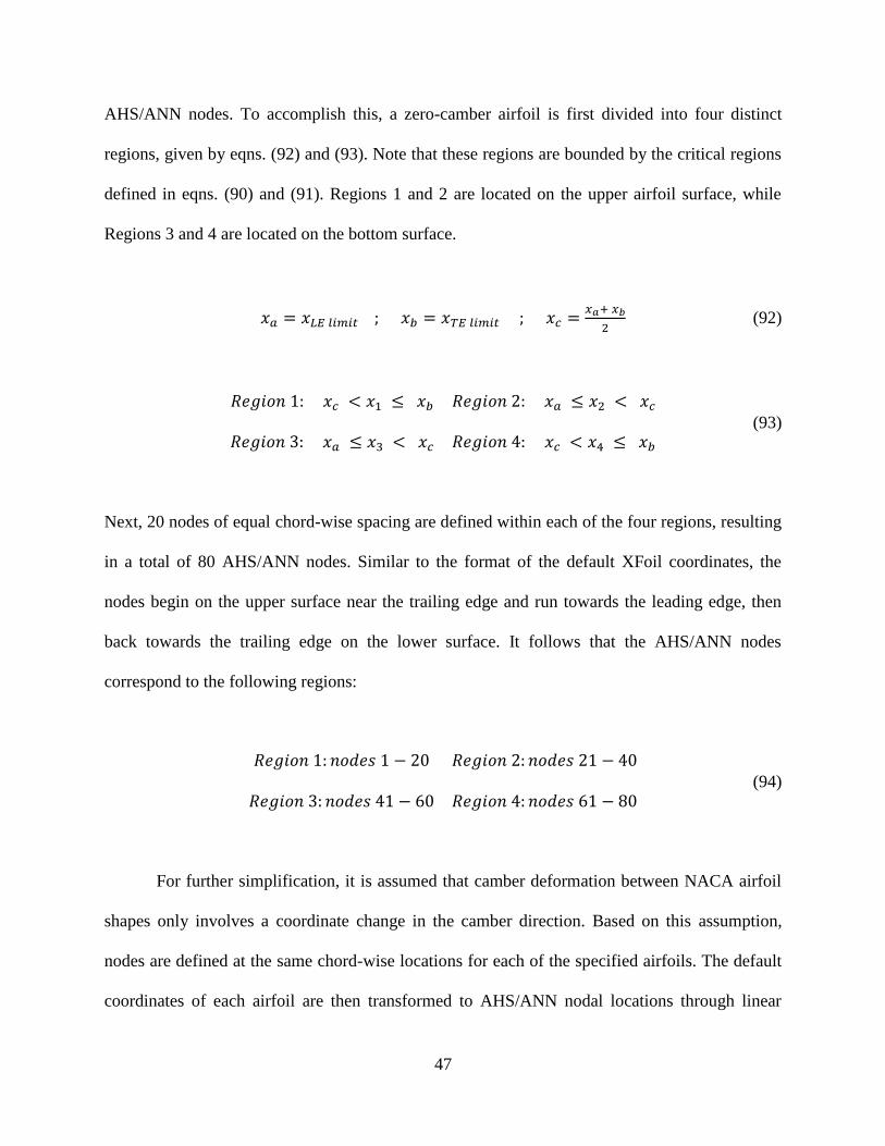
AHS/ANN nodes. To accomplish this, a zero-camber airfoil is first divided into four distinct

regions, given by eqns. (92) and (93). Note that these regions are bounded by the critical regions

defined in eqns. (90) and (91). Regions 1 and 2 are located on the upper airfoil surface, while

Regions 3 and 4 are located on the bottom surface.

(92)

(93)

Next, 20 nodes of equal chord-wise spacing are defined within each of the four regions, resulting

in a total of 80 AHS/ANN nodes. Similar to the format of the default XFoil coordinates, the

nodes begin on the upper surface near the trailing edge and run towards the leading edge, then

back towards the trailing edge on the lower surface. It follows that the AHS/ANN nodes

correspond to the following regions:

(94)

For further simplification, it is assumed that camber deformation between NACA airfoil

shapes only involves a coordinate change in the camber direction. Based on this assumption,

nodes are defined at the same chord-wise locations for each of the specified airfoils. The default

coordinates of each airfoil are then transformed to AHS/ANN nodal locations through linear

48

interpolation. Although this approximation is not entirely accurate, the airfoils examined in this

application are of small enough scale that the error was deemed negligible. Moving forward, it is

of utmost importance to be aware of the AHS/ANN regions and their corresponding nodal

locations. Failure to properly group nodes in the ANN training data according to eqn. (94) will

render the ANN approximation incorrect.

3.2.5 Determining ANN Parameters

The ANN training data is compiled through a process similar to that used to attain the

AHS/ANN node locations. First, XFoil analysis is performed for the desired NACA airfoils and

flow parameters. The default airfoil coordinates are used for this analysis, and the angle of attack

is varied throughout the desired domain in 1 degree increments. The data from the XFoil analysis

is then output to a text file and the relevant values (normalized local velocities and local pressure

coefficients) are transformed to the AHS/ANN nodal locations through linear interpolation. The

overall results are then compiled in matrix form to compose the ANN training data set. Using

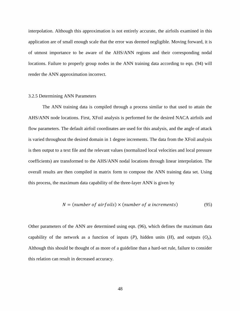
this process, the maximum data capability of the three-layer ANN is given by

(95)

Other parameters of the ANN are determined using eqn. (96), which defines the maximum data

capability of the network as a function of inputs (P), hidden units (H), and outputs (Op).

Although this should be thought of as more of a guideline than a hard-set rule, failure to consider

this relation can result in decreased accuracy.

49

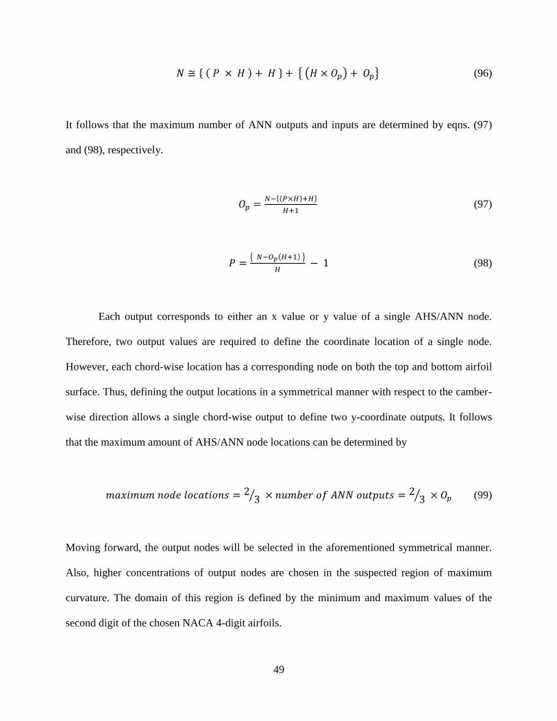
(96)

It follows that the maximum number of ANN outputs and inputs are determined by eqns. (97)

and (98), respectively.

(97)

(98)

Each output corresponds to either an x value or y value of a single AHS/ANN node.

Therefore, two output values are required to define the coordinate location of a single node.

However, each chord-wise location has a corresponding node on both the top and bottom airfoil

surface. Thus, defining the output locations in a symmetrical manner with respect to the camber-

wise direction allows a single chord-wise output to define two y-coordinate outputs. It follows

that the maximum amount of AHS/ANN node locations can be determined by

(99)

Moving forward, the output nodes will be selected in the aforementioned symmetrical manner.

Also, higher concentrations of output nodes are chosen in the suspected region of maximum

curvature. The domain of this region is defined by the minimum and maximum values of the

second digit of the chosen NACA 4-digit airfoils.

50

When defining the quantity of ANN inputs and outputs to use, the main objective is to

define these such as to achieve a sufficiently accurate airfoil shape approximation in the most

efficient manner possible. Referencing eqns. (97) and (98), it can be seen that reducing the

number of inputs allows for an increased number of output values, which can ultimately lead to a

more accurate airfoil shape approximation. It is also important to note that each ANN input used

requires placement of a single AHS in a real-world application. Thus, reducing the number of

AHS required for each system can also reduce cost and labor requirements. However, increasing

the number of output nodes can also lead to the need for a higher maximum data capability. It is

therefore desirable to determine the optimal amount of ANN input and output values to use. The

process for selecting the quantity and locations of the input and output nodes will be more

thoroughly examined through numerical studies in future sections.

3.2.6 Recovering Airfoil Shape

To finalize the AHS/ANN approximation, a method for which to recover the overall

airfoil shape from the ANN nodal approximation was developed. The first step of the airfoil

shape recovery process is to curve-fit the ANN nodal approximation, which is lacking the critical

regions near the leading and trailing edges. This is done by using a cubic regression function on

the top and bottom sides of the ANN approximation individually, specifically the “spline”

function in MATLAB.

The next step of the shape recovery process is to recover the trailing edge. This is done

by defining two trailing edge points

(100)

51

and then individually curve-fitting the top and bottom sides of the trailing edge, once again using

the “spline” function in MATLAB. These points are defined to eliminate the previously

mentioned stagnation effects at the trailing edge during XFoil analysis.

Recovery of the leading edge presented more difficulty and therefore required a trial and

error approach with various curve fitting methods. Ultimately, the method that was decided upon

involves first adding in a defined leading edge point at

(101)

With this point defined, the top and bottom sides of the leading edge are then curve fit

separately, once again using the “spline” function in MATLAB. Once the leading and trailing

edges are recovered, all six “spline” functions are combined to form the initial airfoil

approximation. The initial overall airfoil approximation is then input to XFoil to redefine the

leading edge radius and eliminate the discontinuity that is present in the initial leading edge

approximation. The overall airfoil approximation is then considered complete.

3.2.7 Aerodynamic Analysis and Extracting Camber Line

The accuracy of the AHS/ANN approximation is first verified through aerodynamic

analysis in XFoil. This is done by importing the airfoil shape approximation into XFoil and

performing analysis at the specified test conditions. The relevant aerodynamic results (lift

coefficient, moment coefficient, and pressure distribution) are then recorded for comparison with

that of the test airfoil.

52

In order to compare the results of the AHS/ANN airfoil approximation with that of the

aerodynamic formulation, the section lift and moment coefficients are calculated from the mid-

chord lift and moment about the aerodynamic center location. These values are then compared to

those obtained from XFoil analysis of the AHS/ANN approximation.

Another approach is to model the airfoil approximation as a thin airfoil. To accomplish

this, the mean camber line is extracted by calculating the mean camber-wise shape along the

entire chord length. The mean camber line is then used to define the AHS/ANN airfoil shape

approximation for such comparisons.

53

CHAPTER 4

NUMERICAL STUDIES

4.1 Modified Finite-State Inflow Formulation

The modified finite-state inflow formulation derived in Chapter 3 can be utilized for a

wide range of applications, many of which contain unsteady aerodynamic properties. This

unsteadiness can be accounted for in the λ0 term of eqn. (20), which can be defined in terms of

the Theodorsen function. However, the desired use of the modified theory in this application is

for verification of the aerodynamic results from the AHS/ANN system. Therefore, unsteady

effects are not examined in the presented numerical studies, and the airfoil motions are modeled

as quasi-steady.

4.1.1 Test Case 4.1a – Quasi-Steady Rigid Airfoil Application

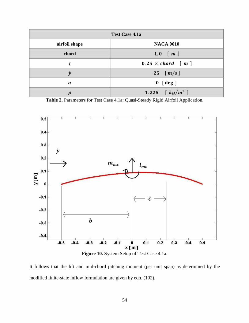
As an initial analysis of the modified finite-state inflow formulation, a rigid airfoil with a

constant camber deformation is examined. The camber-deformed airfoil is chosen to be a NACA

9610 airfoil of chord length , and is represented by the mean camber line. The airfoil

is placed along the x axis with the leading edge located at and the trailing edge

at , as illustrated in Fig. 10. The flow is considered to be quasi-steady, and therefore the

airfoil is defined to have no pitching or plunging motion.

54

Test Case 4.1a

airfoil shape NACA 9610

chord

Table 2. Parameters for Test Case 4.1a: Quasi-Steady Rigid Airfoil Application.

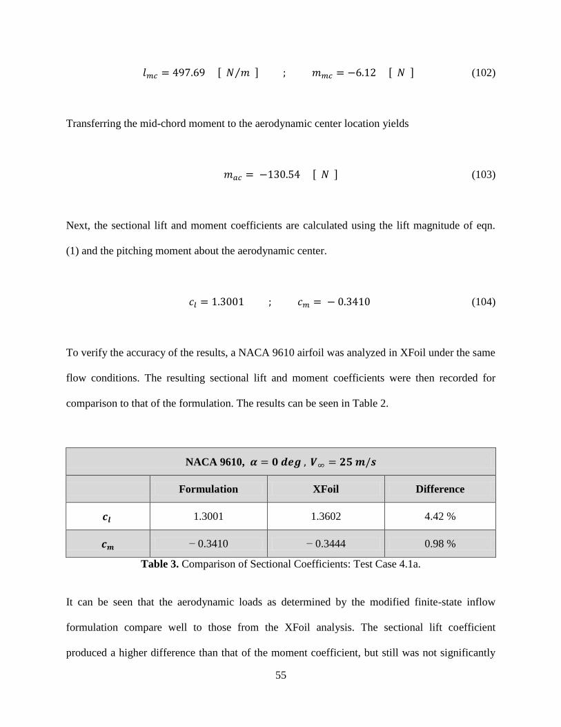
It follows that the lift and mid-chord pitching moment (per unit span) as determined by the

modified finite-state inflow formulation are given by eqn. (102).

Figure 10. System Setup of Test Case 4.1a.

55

(102)

Transferring the mid-chord moment to the aerodynamic center location yields

(103)

Next, the sectional lift and moment coefficients are calculated using the lift magnitude of eqn.

(1) and the pitching moment about the aerodynamic center.

(104)

To verify the accuracy of the results, a NACA 9610 airfoil was analyzed in XFoil under the same

flow conditions. The resulting sectional lift and moment coefficients were then recorded for

comparison to that of the formulation. The results can be seen in Table 2.

NACA 9610,

Formulation XFoil Difference

1.3001 1.3602 4.42 %

− 0.3410 − 0.3444 0.98 %

Table 3. Comparison of Sectional Coefficients: Test Case 4.1a.

It can be seen that the aerodynamic loads as determined by the modified finite-state inflow

formulation compare well to those from the XFoil analysis. The sectional lift coefficient

produced a higher difference than that of the moment coefficient, but still was not significantly

56

high. Because the airfoils being considered are cambered, the most important parameter in

determining the accuracy of the aerodynamic formulation is the sectional moment coefficient

about the aerodynamic center.

4.1.2 Test Case 4.1b – Camber Actuation

Ultimately, anti-symmetric camber actuations over the length of a morphing aircraft wing

can be utilized to generate roll, pitch, and yaw. Due to the coupling of the wing deformation and

vehicle rigid-body motions, performing a single one of these rigid-body motions will cause

excitement in the remaining two. In order to analyze the effect of these motions, one must be

able to track the aerodynamic loads throughout the actuation process. The airfoil to be examined

in this test case has a chord length of 1 m and is initially oriented such that the leading edge is

located at and the trailing edge is located at . The maximum camber shape is

defined by the mean camber line of a NACA 9310 airfoil. To demonstrate the ability to track

aerodynamic loads throughout a camber actuation process, a piece-wise camber actuation

function is applied to the airfoil over a given time interval in order to simulate actuation from an

initial camber shape to a desired camber shape. The camber actuation function is given in eqn.

(4) and has a defined frequency of , resulting in a period of .

(105)

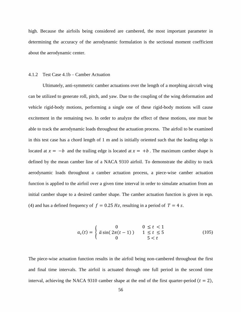
The piece-wise actuation function results in the airfoil being non-cambered throughout the first

and final time intervals. The airfoil is actuated through one full period in the second time

interval, achieving the NACA 9310 camber shape at the end of the first quarter-period ,

57

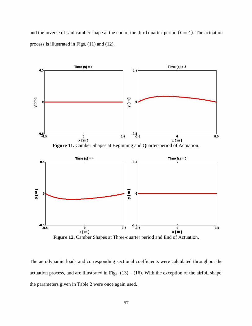
and the inverse of said camber shape at the end of the third quarter-period . The actuation

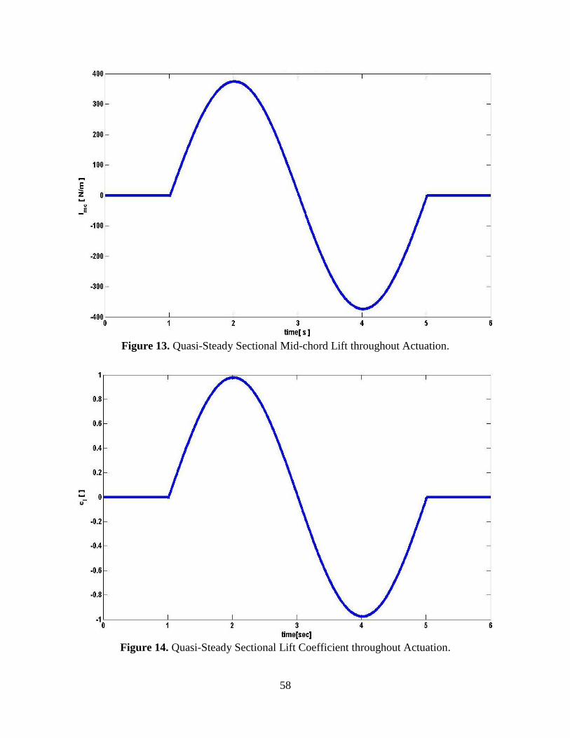
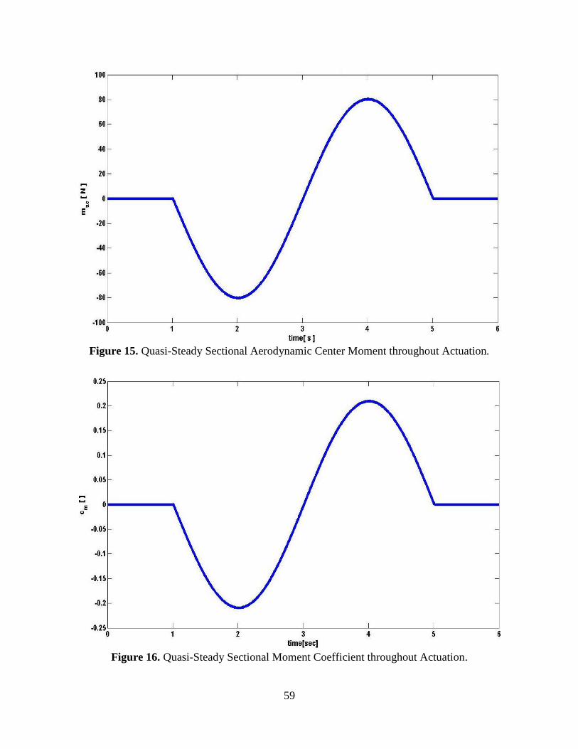
process is illustrated in Figs. (11) and (12).

The aerodynamic loads and corresponding sectional coefficients were calculated throughout the

actuation process, and are illustrated in Figs. (13) – (16). With the exception of the airfoil shape,

the parameters given in Table 2 were once again used.

Figure 12. Camber Shapes at Three-quarter period and End of Actuation.

Figure 11. Camber Shapes at Beginning and Quarter-period of Actuation.

58

Figure 14. Quasi-Steady Sectional Lift Coefficient throughout Actuation.

Figure 13. Quasi-Steady Sectional Mid-chord Lift throughout Actuation.

59

Figure 16. Quasi-Steady Sectional Moment Coefficient throughout Actuation.

Figure 15. Quasi-Steady Sectional Aerodynamic Center Moment throughout Actuation.

60

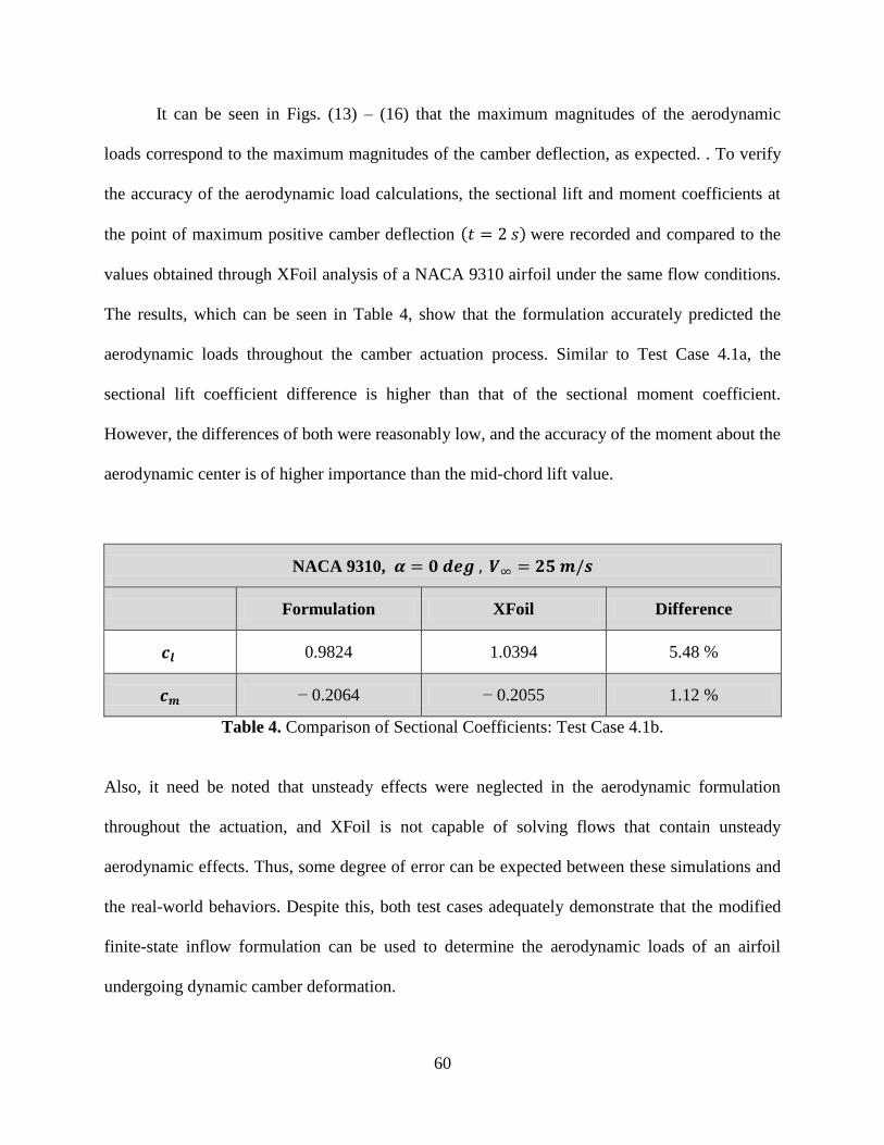
It can be seen in Figs. (13) – (16) that the maximum magnitudes of the aerodynamic

loads correspond to the maximum magnitudes of the camber deflection, as expected. . To verify

the accuracy of the aerodynamic load calculations, the sectional lift and moment coefficients at

the point of maximum positive camber deflection were recorded and compared to the

values obtained through XFoil analysis of a NACA 9310 airfoil under the same flow conditions.

The results, which can be seen in Table 4, show that the formulation accurately predicted the

aerodynamic loads throughout the camber actuation process. Similar to Test Case 4.1a, the

sectional lift coefficient difference is higher than that of the sectional moment coefficient.

However, the differences of both were reasonably low, and the accuracy of the moment about the

aerodynamic center is of higher importance than the mid-chord lift value.

NACA 9310,

Formulation XFoil Difference

0.9824 1.0394 5.48 %

− 0.2064 − 0.2055 1.12 %

Table 4. Comparison of Sectional Coefficients: Test Case 4.1b.

Also, it need be noted that unsteady effects were neglected in the aerodynamic formulation

throughout the actuation, and XFoil is not capable of solving flows that contain unsteady

aerodynamic effects. Thus, some degree of error can be expected between these simulations and

the real-world behaviors. Despite this, both test cases adequately demonstrate that the modified

finite-state inflow formulation can be used to determine the aerodynamic loads of an airfoil

undergoing dynamic camber deformation.

61

4.2 AHS/ANN System – Airfoil Shape Determination

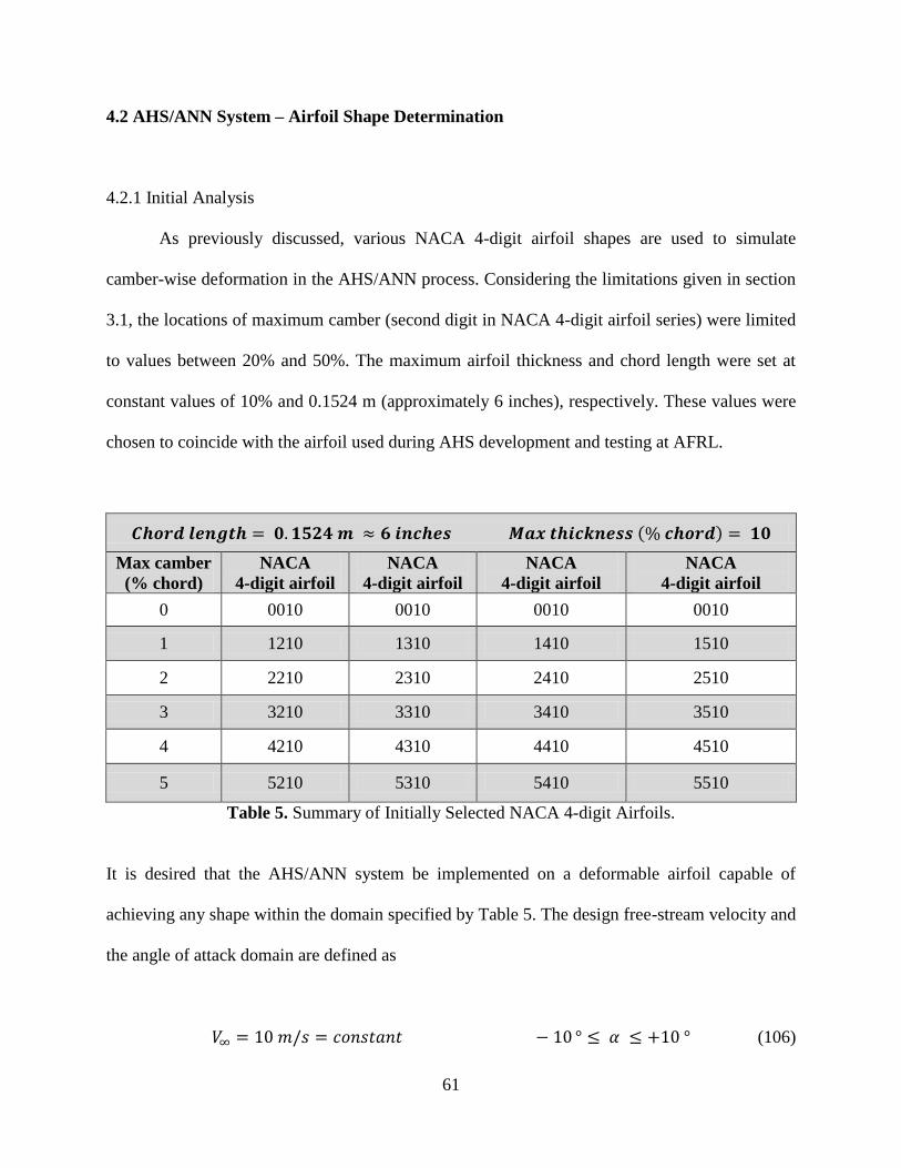
4.2.1 Initial Analysis

As previously discussed, various NACA 4-digit airfoil shapes are used to simulate

camber-wise deformation in the AHS/ANN process. Considering the limitations given in section

3.1, the locations of maximum camber (second digit in NACA 4-digit airfoil series) were limited

to values between 20% and 50%. The maximum airfoil thickness and chord length were set at

constant values of 10% and 0.1524 m (approximately 6 inches), respectively. These values were

chosen to coincide with the airfoil used during AHS development and testing at AFRL.

Max camber

(% chord)

NACA

4-digit airfoil

NACA

4-digit airfoil

NACA

4-digit airfoil

NACA

4-digit airfoil

0 0010 0010 0010 0010

1 1210 1310 1410 1510

2 2210 2310 2410 2510

3 3210 3310 3410 3510

4 4210 4310 4410 4510

5 5210 5310 5410 5510

Table 5. Summary of Initially Selected NACA 4-digit Airfoils.

It is desired that the AHS/ANN system be implemented on a deformable airfoil capable of

achieving any shape within the domain specified by Table 5. The design free-stream velocity and

the angle of attack domain are defined as

(106)

62

The current AHS cannot perform effectively at flow velocities greater than .

Thus, the normalized local velocity limit as determined by eqn. (88) is

(107)

As an initial examination of the aforementioned critical regions, a NACA 5410 airfoil

was selected for analysis in XFoil. The free-stream velocity was held constant at the design value

and the angle of attack was varied from to in 5 degree increments.

The airfoil coordinates and corresponding local velocities were then output for each airfoil. Also,

the local pressure coefficients were output and used to verify the accuracy of the local velocity

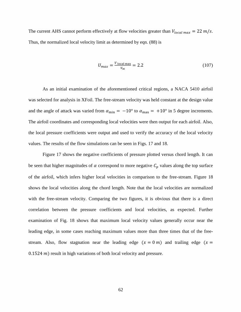
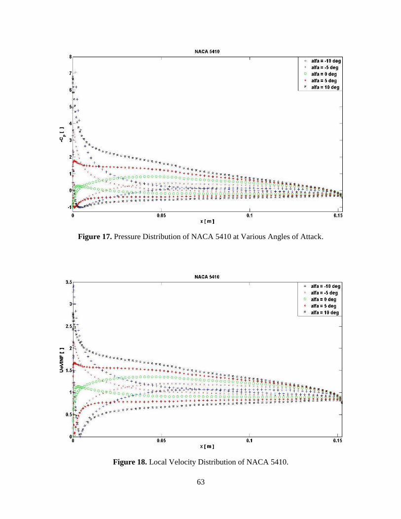
values. The results of the flow simulations can be seen in Figs. 17 and 18.

Figure 17 shows the negative coefficients of pressure plotted versus chord length. It can

be seen that higher magnitudes of correspond to more negative values along the top surface

of the airfoil, which infers higher local velocities in comparison to the free-stream. Figure 18

shows the local velocities along the chord length. Note that the local velocities are normalized

with the free-stream velocity. Comparing the two figures, it is obvious that there is a direct

correlation between the pressure coefficients and local velocities, as expected. Further

examination of Fig. 18 shows that maximum local velocity values generally occur near the

leading edge, in some cases reaching maximum values more than three times that of the free-

stream. Also, flow stagnation near the leading edge and trailing edge

result in high variations of both local velocity and pressure.

63

Figure 18. Local Velocity Distribution of NACA 5410.

Figure 17. Pressure Distribution of NACA 5410 at Various Angles of Attack.

64

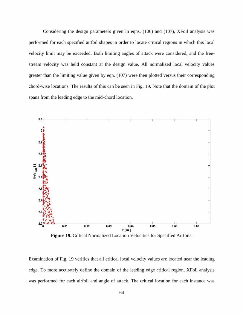
Considering the design parameters given in eqns. (106) and (107), XFoil analysis was

performed for each specified airfoil shapes in order to locate critical regions in which this local

velocity limit may be exceeded. Both limiting angles of attack were considered, and the free-

stream velocity was held constant at the design value. All normalized local velocity values

greater than the limiting value given by eqn. (107) were then plotted versus their corresponding

chord-wise locations. The results of this can be seen in Fig. 19. Note that the domain of the plot

spans from the leading edge to the mid-chord location.

Examination of Fig. 19 verifies that all critical local velocity values are located near the leading

edge. To more accurately define the domain of the leading edge critical region, XFoil analysis

was performed for each airfoil and angle of attack. The critical location for each instance was

Figure 19. Critical Normalized Location Velocities for Specified Airfoils

65

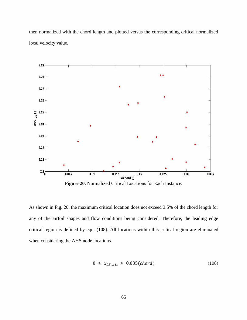
then normalized with the chord length and plotted versus the corresponding critical normalized

local velocity value.

As shown in Fig. 20, the maximum critical location does not exceed 3.5% of the chord length for

any of the airfoil shapes and flow conditions being considered. Therefore, the leading edge

critical region is defined by eqn. (108). All locations within this critical region are eliminated

when considering the AHS node locations.

(108)

Figure 20. Normalized Critical Locations for Each Instance.

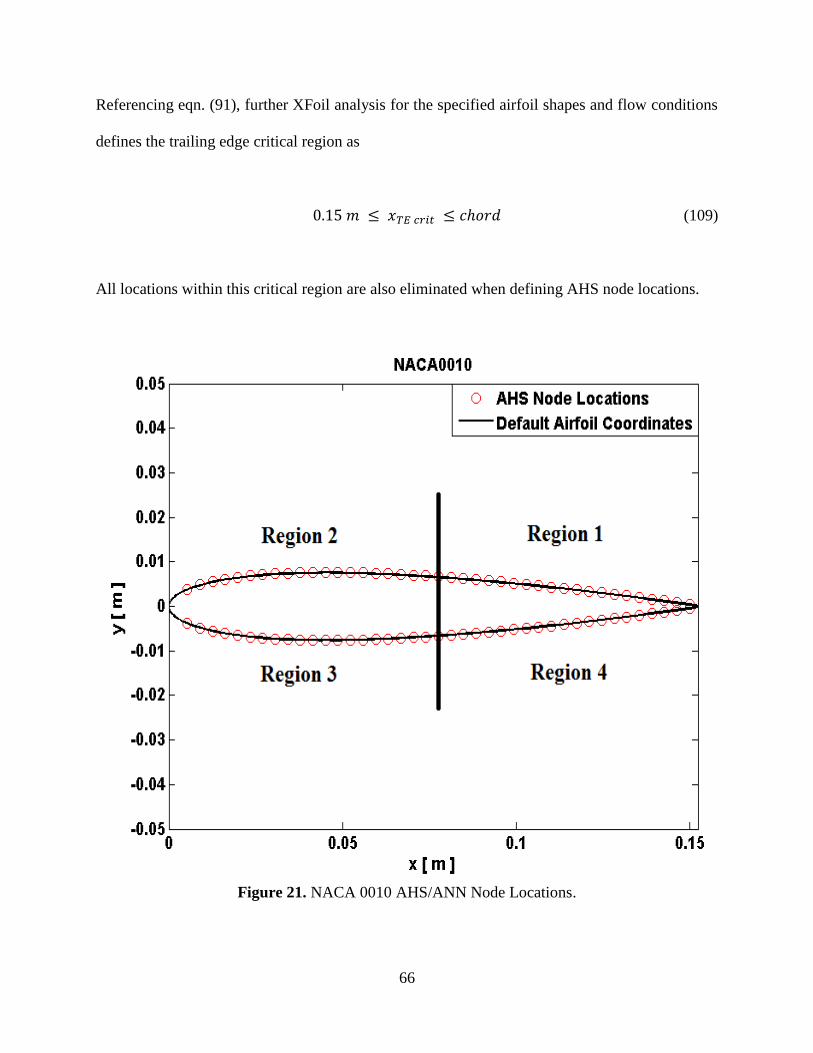
66

Referencing eqn. (91), further XFoil analysis for the specified airfoil shapes and flow conditions

defines the trailing edge critical region as

(109)

All locations within this critical region are also eliminated when defining AHS node locations.

Figure 21. NACA 0010 AHS/ANN Node Locations.

67

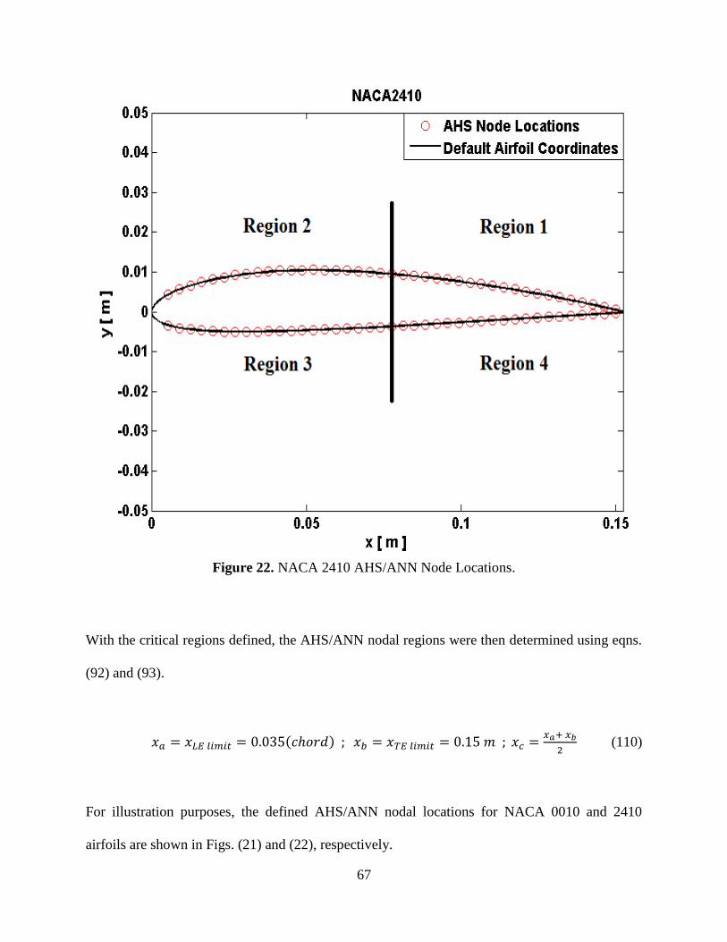
With the critical regions defined, the AHS/ANN nodal regions were then determined using eqns.

(92) and (93).

(110)

For illustration purposes, the defined AHS/ANN nodal locations for NACA 0010 and 2410

airfoils are shown in Figs. (21) and (22), respectively.

Figure 22. NACA 2410 AHS/ANN Node Locations.

68

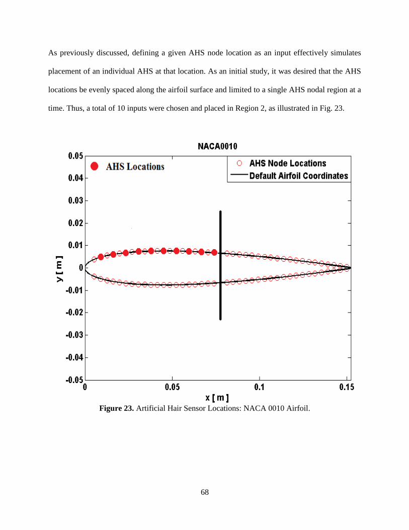
As previously discussed, defining a given AHS node location as an input effectively simulates

placement of an individual AHS at that location. As an initial study, it was desired that the AHS

locations be evenly spaced along the airfoil surface and limited to a single AHS nodal region at a

time. Thus, a total of 10 inputs were chosen and placed in Region 2, as illustrated in Fig. 23.

Figure 23. Artificial Hair Sensor Locations: NACA 0010 Airfoil.

69

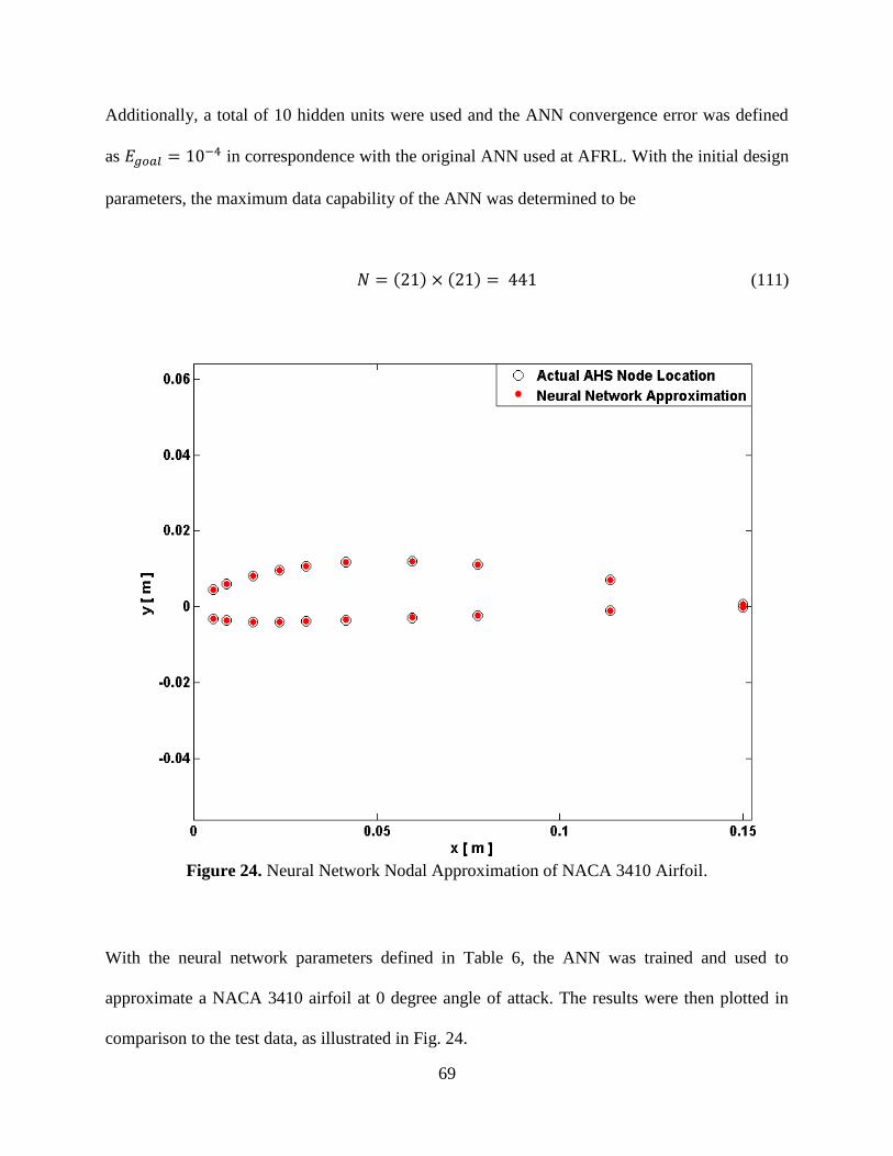
Additionally, a total of 10 hidden units were used and the ANN convergence error was defined

as in correspondence with the original ANN used at AFRL. With the initial design

parameters, the maximum data capability of the ANN was determined to be

(111)

With the neural network parameters defined in Table 6, the ANN was trained and used to

approximate a NACA 3410 airfoil at 0 degree angle of attack. The results were then plotted in

comparison to the test data, as illustrated in Fig. 24.

Figure 24. Neural Network Nodal Approximation of NACA 3410 Airfoil.

70

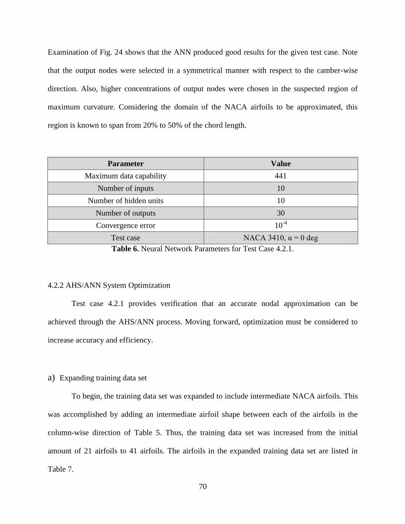
Examination of Fig. 24 shows that the ANN produced good results for the given test case. Note

that the output nodes were selected in a symmetrical manner with respect to the camber-wise

direction. Also, higher concentrations of output nodes were chosen in the suspected region of

maximum curvature. Considering the domain of the NACA airfoils to be approximated, this

region is known to span from 20% to 50% of the chord length.

Parameter Value

Maximum data capability 441

Number of inputs 10

Number of hidden units 10

Number of outputs 30

Convergence error 10-4

Test case NACA 3410, α = 0 deg

Table 6. Neural Network Parameters for Test Case 4.2.1.

4.2.2 AHS/ANN System Optimization

Test case 4.2.1 provides verification that an accurate nodal approximation can be

achieved through the AHS/ANN process. Moving forward, optimization must be considered to

increase accuracy and efficiency.

a) Expanding training data set

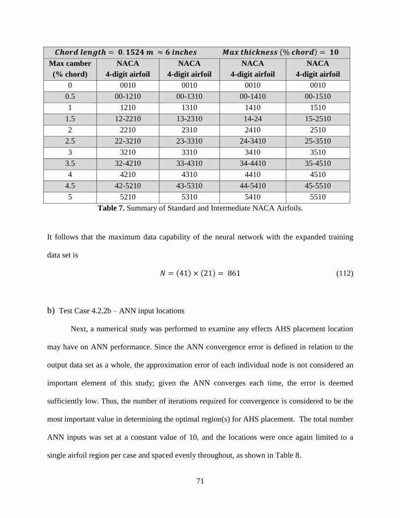
To begin, the training data set was expanded to include intermediate NACA airfoils. This

was accomplished by adding an intermediate airfoil shape between each of the airfoils in the

column-wise direction of Table 5. Thus, the training data set was increased from the initial

amount of 21 airfoils to 41 airfoils. The airfoils in the expanded training data set are listed in

Table 7.

71

Max camber

(% chord)

NACA

4-digit airfoil

NACA

4-digit airfoil

NACA

4-digit airfoil

NACA

4-digit airfoil

0 0010 0010 0010 0010

0.5 00-1210 00-1310 00-1410 00-1510

1 1210 1310 1410 1510

1.5 12-2210 13-2310 14-24 15-2510

2 2210 2310 2410 2510

2.5 22-3210 23-3310 24-3410 25-3510

3 3210 3310 3410 3510

3.5 32-4210 33-4310 34-4410 35-4510

4 4210 4310 4410 4510

4.5 42-5210 43-5310 44-5410 45-5510

5 5210 5310 5410 5510

Table 7. Summary of Standard and Intermediate NACA Airfoils.

It follows that the maximum data capability of the neural network with the expanded training

data set is

(112)

b) Test Case 4.2.2b – ANN input locations

Next, a numerical study was performed to examine any effects AHS placement location

may have on ANN performance. Since the ANN convergence error is defined in relation to the

output data set as a whole, the approximation error of each individual node is not considered an

important element of this study; given the ANN converges each time, the error is deemed

sufficiently low. Thus, the number of iterations required for convergence is considered to be the

most important value in determining the optimal region(s) for AHS placement. The total number

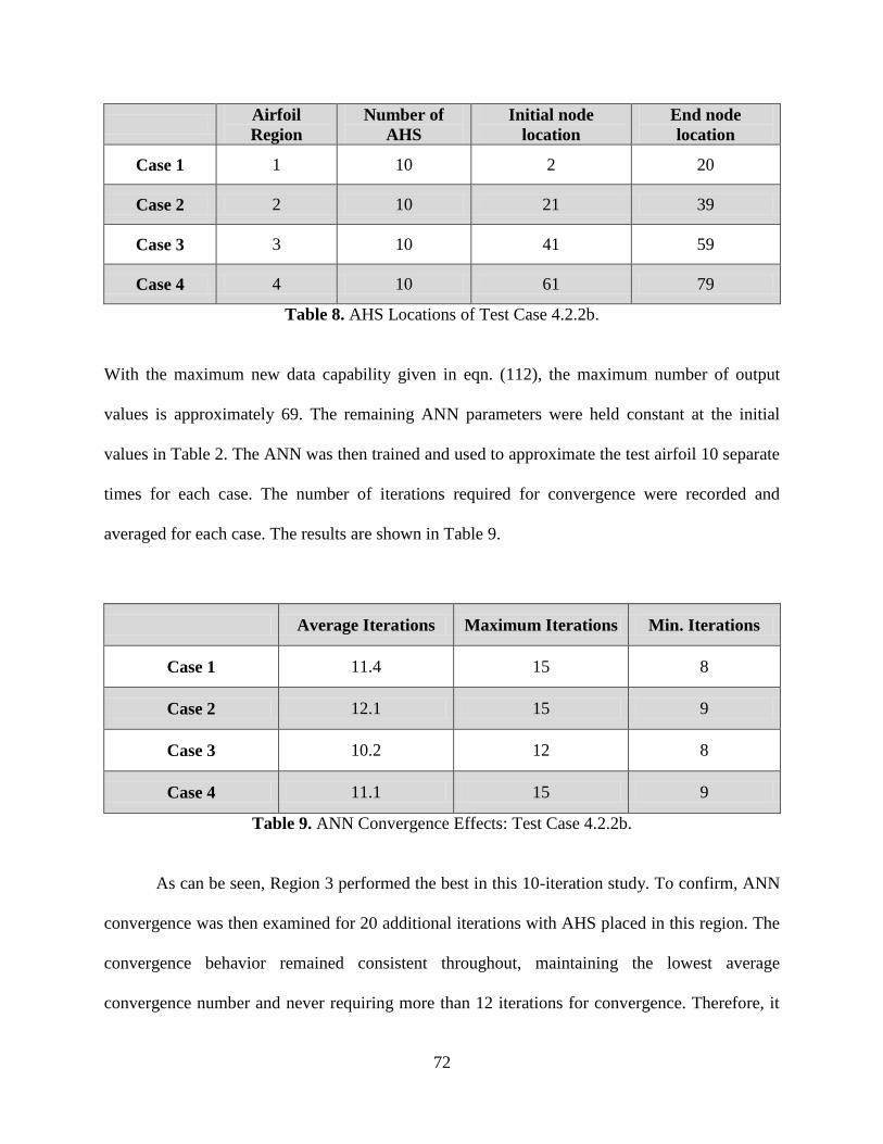
ANN inputs was set at a constant value of 10, and the locations were once again limited to a

single airfoil region per case and spaced evenly throughout, as shown in Table 8.

72

Airfoil

Region

Number of

AHS

Initial node

location

End node

location

Case 1 1 10 2 20

Case 2 2 10 21 39

Case 3 3 10 41 59

Case 4 4 10 61 79

Table 8. AHS Locations of Test Case 4.2.2b.

With the maximum new data capability given in eqn. (112), the maximum number of output

values is approximately 69. The remaining ANN parameters were held constant at the initial

values in Table 2. The ANN was then trained and used to approximate the test airfoil 10 separate

times for each case. The number of iterations required for convergence were recorded and

averaged for each case. The results are shown in Table 9.

Average Iterations Maximum Iterations Min. Iterations

Case 1 11.4 15 8

Case 2 12.1 15 9

Case 3 10.2 12 8

Case 4 11.1 15 9

Table 9. ANN Convergence Effects: Test Case 4.2.2b.

As can be seen, Region 3 performed the best in this 10-iteration study. To confirm, ANN

convergence was then examined for 20 additional iterations with AHS placed in this region. The

convergence behavior remained consistent throughout, maintaining the lowest average

convergence number and never requiring more than 12 iterations for convergence. Therefore, it

73

was determined that the optimal region for AHS placement is Region 3. It should be noted that

the number of iterations required for convergence is directly affected by the number of input and

output nodes selected. Thus, although all four cases produced similar results, these differences

could potentially be amplified by altering either of these parameters. Although placing AHS in

any of the other three regions should not be considered completely off limits, Region 3 is used in

future applications.

c) Test Case 4.2.2c – AHS/ANN inputs and quantity

To determine the optimum number of ANN inputs, a numerical study similar to that of

Test Case 4.2.2b was performed. Three separate configurations were examined by varying the

quantity of ANN inputs and increasing the number of outputs in accordance with eqn. (96), as

outlined in Table 10. The remaining ANN parameters were held constant. The configurations

were defined such that the maximum amount of the Region 3 was spanned as possible while still

maintaining even spacing of the ANN input locations.

Configuration No. of AHS AHS

spacing

Initial node

location

End node

location

No. of ANN

outputs

1 10 2 41 59 30

2 7 3 41 59 33

3 4 6 41 59 36

Table 10. Parameters for Test Case 4.2.2c.

Performance of the ANN was once again analyzed by examining the number of iterations

required for convergence. The ANN was trained and used to approximate the test airfoil 10

times, recording the required number of iterations for convergence and averaging the values for

74

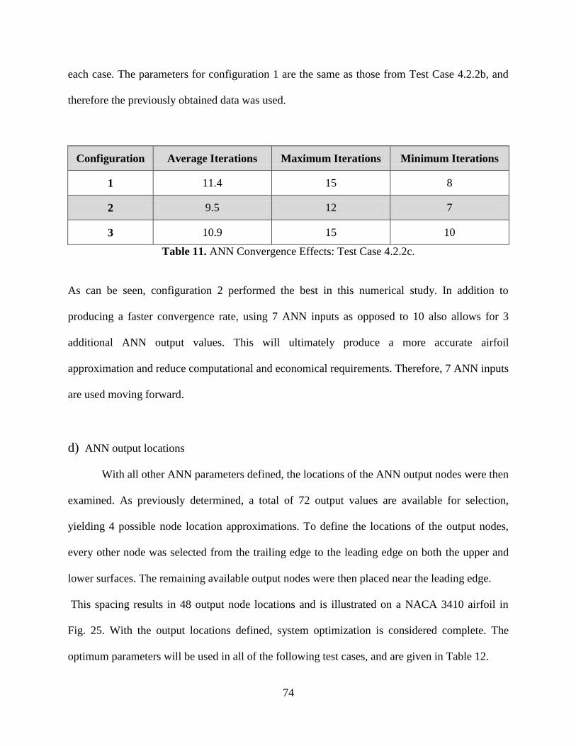
each case. The parameters for configuration 1 are the same as those from Test Case 4.2.2b, and

therefore the previously obtained data was used.

Configuration Average Iterations Maximum Iterations Minimum Iterations

1 11.4 15 8

2 9.5 12 7

3 10.9 15 10

Table 11. ANN Convergence Effects: Test Case 4.2.2c.

As can be seen, configuration 2 performed the best in this numerical study. In addition to

producing a faster convergence rate, using 7 ANN inputs as opposed to 10 also allows for 3

additional ANN output values. This will ultimately produce a more accurate airfoil

approximation and reduce computational and economical requirements. Therefore, 7 ANN inputs

are used moving forward.

d) ANN output locations

With all other ANN parameters defined, the locations of the ANN output nodes were then

examined. As previously determined, a total of 72 output values are available for selection,

yielding 4 possible node location approximations. To define the locations of the output nodes,

every other node was selected from the trailing edge to the leading edge on both the upper and

lower surfaces. The remaining available output nodes were then placed near the leading edge.

This spacing results in 48 output node locations and is illustrated on a NACA 3410 airfoil in

Fig. 25. With the output locations defined, system optimization is considered complete. The

optimum parameters will be used in all of the following test cases, and are given in Table 12.

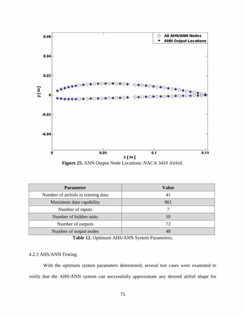
75

Parameter Value

Number of airfoils in training data 41

Maximum data capability 861

Number of inputs 7

Number of hidden units 10

Number of outputs 72

Number of output nodes 48

Table 12. Optimum AHS/ANN System Parameters.

4.2.3 AHS/ANN Testing

With the optimum system parameters determined, several test cases were examined to

verify that the AHS/ANN system can successfully approximate any desired airfoil shape for

Figure 25. ANN Output Node Locations: NACA 3410 Airfoil.

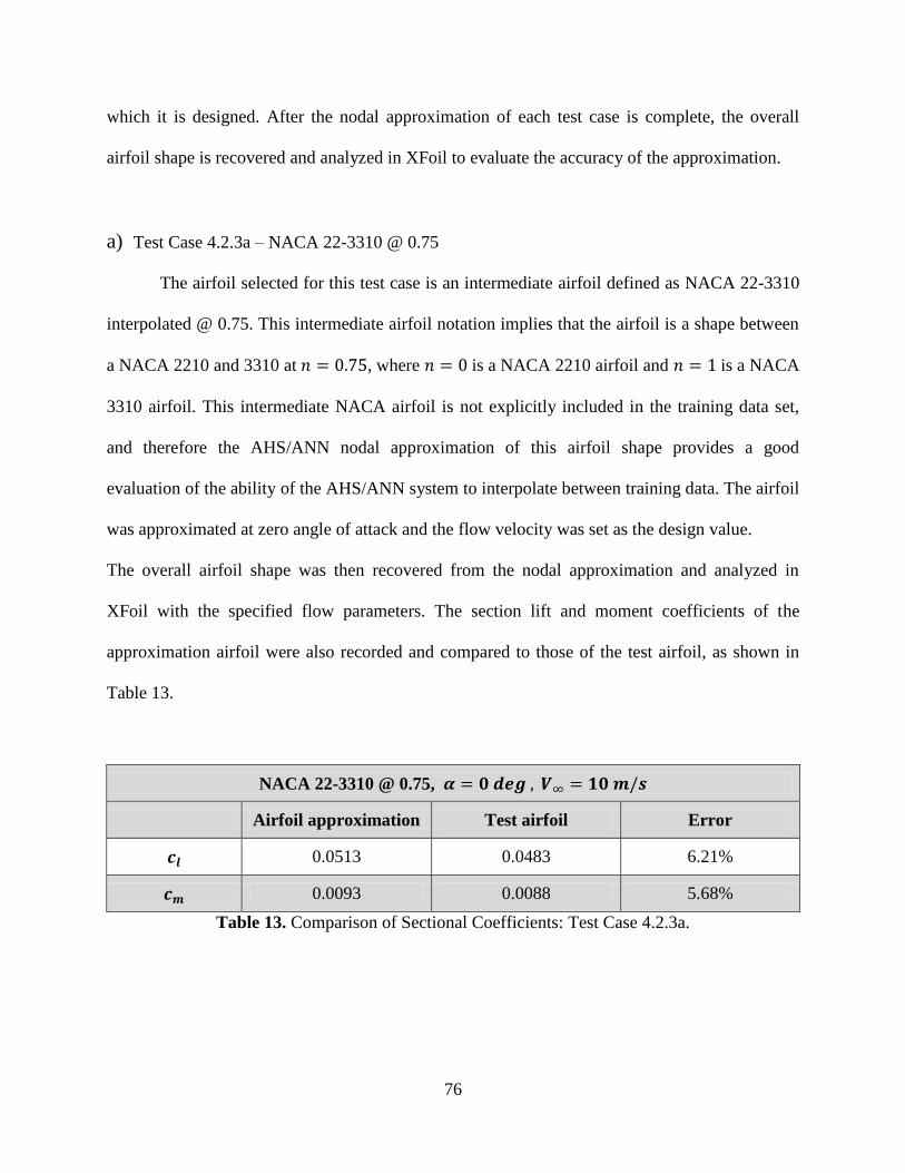
76

which it is designed. After the nodal approximation of each test case is complete, the overall

airfoil shape is recovered and analyzed in XFoil to evaluate the accuracy of the approximation.

a) Test Case 4.2.3a – NACA 22-3310 @ 0.75

The airfoil selected for this test case is an intermediate airfoil defined as NACA 22-3310

interpolated @ 0.75. This intermediate airfoil notation implies that the airfoil is a shape between

a NACA 2210 and 3310 at , where is a NACA 2210 airfoil and is a NACA

3310 airfoil. This intermediate NACA airfoil is not explicitly included in the training data set,

and therefore the AHS/ANN nodal approximation of this airfoil shape provides a good

evaluation of the ability of the AHS/ANN system to interpolate between training data. The airfoil

was approximated at zero angle of attack and the flow velocity was set as the design value.

The overall airfoil shape was then recovered from the nodal approximation and analyzed in

XFoil with the specified flow parameters. The section lift and moment coefficients of the

approximation airfoil were also recorded and compared to those of the test airfoil, as shown in

Table 13.

NACA 22-3310 @ 0.75,

Airfoil approximation Test airfoil Error

0.0513 0.0483 6.21%

0.0093 0.0088 5.68%

Table 13. Comparison of Sectional Coefficients: Test Case 4.2.3a.

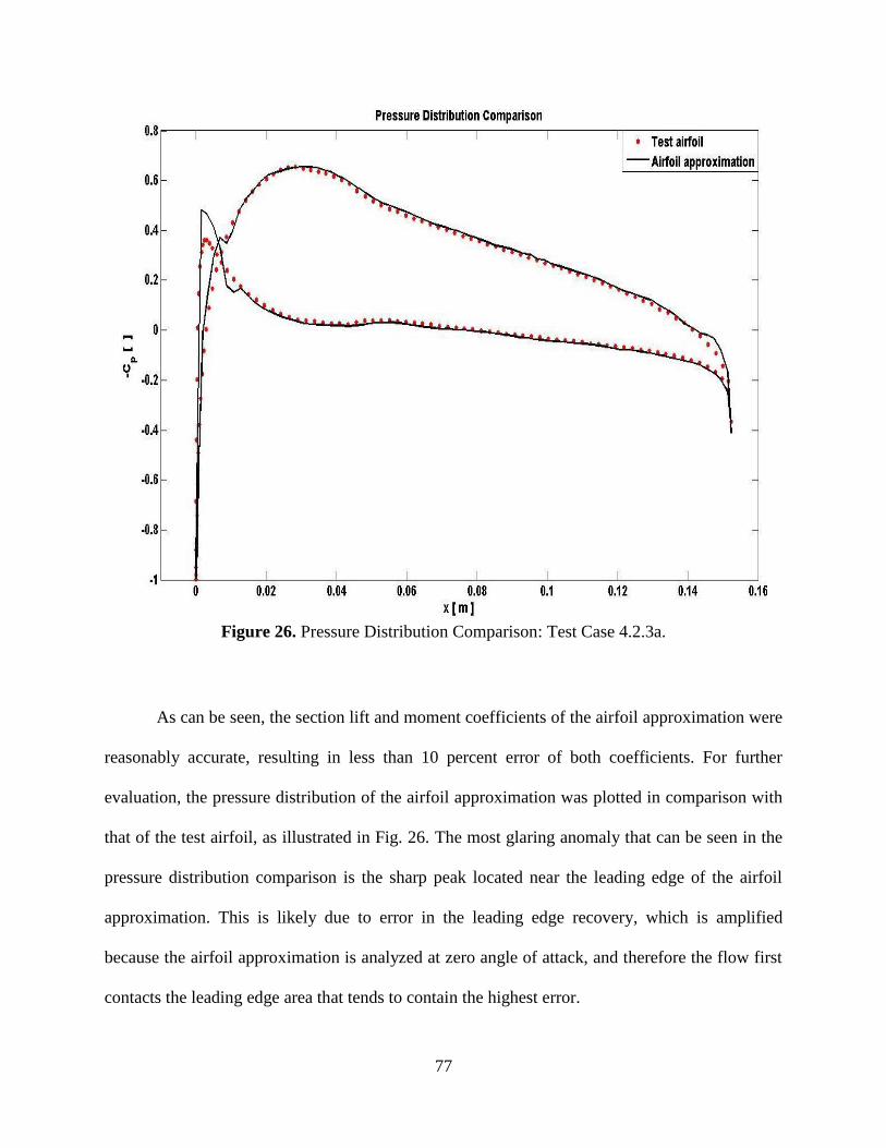
77

As can be seen, the section lift and moment coefficients of the airfoil approximation were

reasonably accurate, resulting in less than 10 percent error of both coefficients. For further

evaluation, the pressure distribution of the airfoil approximation was plotted in comparison with

that of the test airfoil, as illustrated in Fig. 26. The most glaring anomaly that can be seen in the

pressure distribution comparison is the sharp peak located near the leading edge of the airfoil

approximation. This is likely due to error in the leading edge recovery, which is amplified

because the airfoil approximation is analyzed at zero angle of attack, and therefore the flow first

contacts the leading edge area that tends to contain the highest error.

Figure 26. Pressure Distribution Comparison: Test Case 4.2.3a.

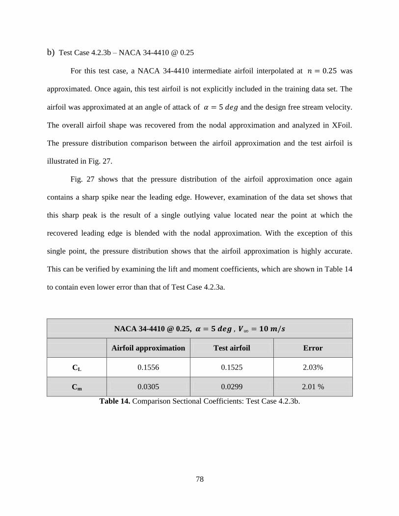
78

b) Test Case 4.2.3b – NACA 34-4410 @ 0.25

For this test case, a NACA 34-4410 intermediate airfoil interpolated at was

approximated. Once again, this test airfoil is not explicitly included in the training data set. The

airfoil was approximated at an angle of attack of and the design free stream velocity.

The overall airfoil shape was recovered from the nodal approximation and analyzed in XFoil.

The pressure distribution comparison between the airfoil approximation and the test airfoil is


Fig. 27 shows that the pressure distribution of the airfoil approximation once again

contains a sharp spike near the leading edge. However, examination of the data set shows that

this sharp peak is the result of a single outlying value located near the point at which the

recovered leading edge is blended with the nodal approximation. With the exception of this

single point, the pressure distribution shows that the airfoil approximation is highly accurate.

This can be verified by examining the lift and moment coefficients, which are shown in Table 14

to contain even lower error than that of Test Case 4.2.3a.

NACA 34-4410 @ 0.25,


CL 0.1556 0.1525 2.03%

Cm 0.0305 0.0299 2.01 %

Table 14. Comparison Sectional Coefficients: Test Case 4.2.3b.

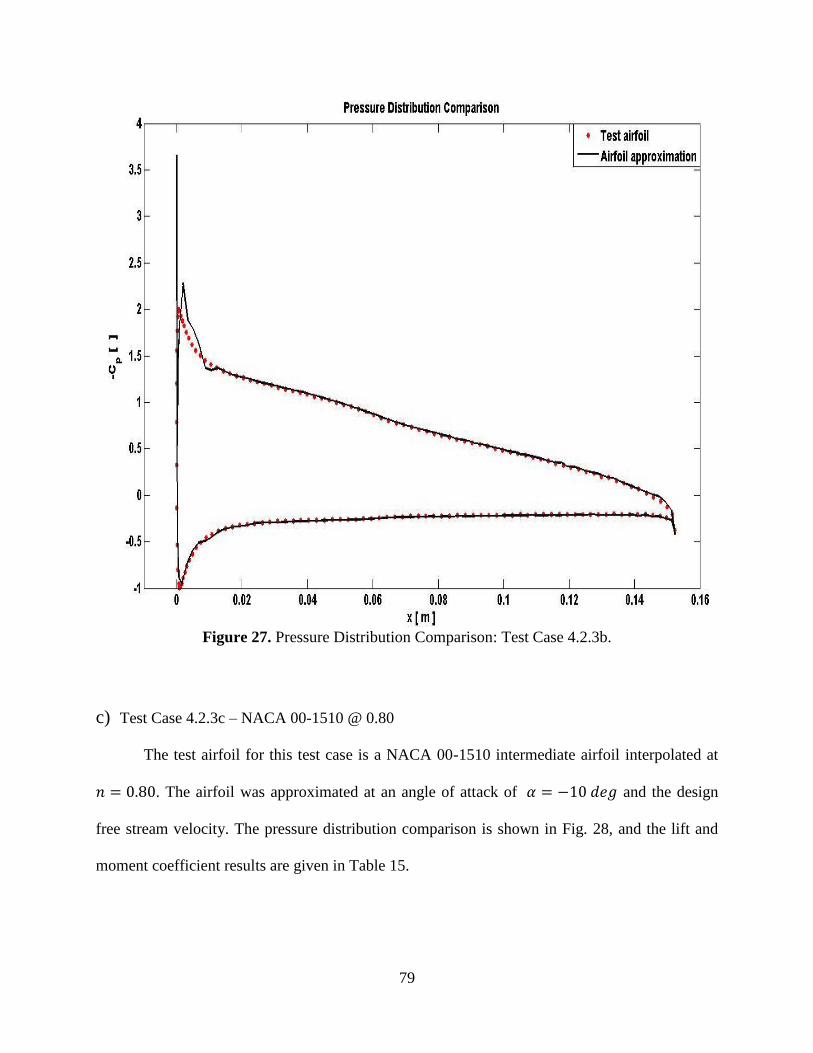
79

c) Test Case 4.2.3c – NACA 00-1510 @ 0.80

The test airfoil for this test case is a NACA 00-1510 intermediate airfoil interpolated at

. The airfoil was approximated at an angle of attack of and the design

free stream velocity. The pressure distribution comparison is shown in Fig. 28, and the lift and

moment coefficient results are given in Table 15.

Figure 27. Pressure Distribution Comparison: Test Case 4.2.3b.

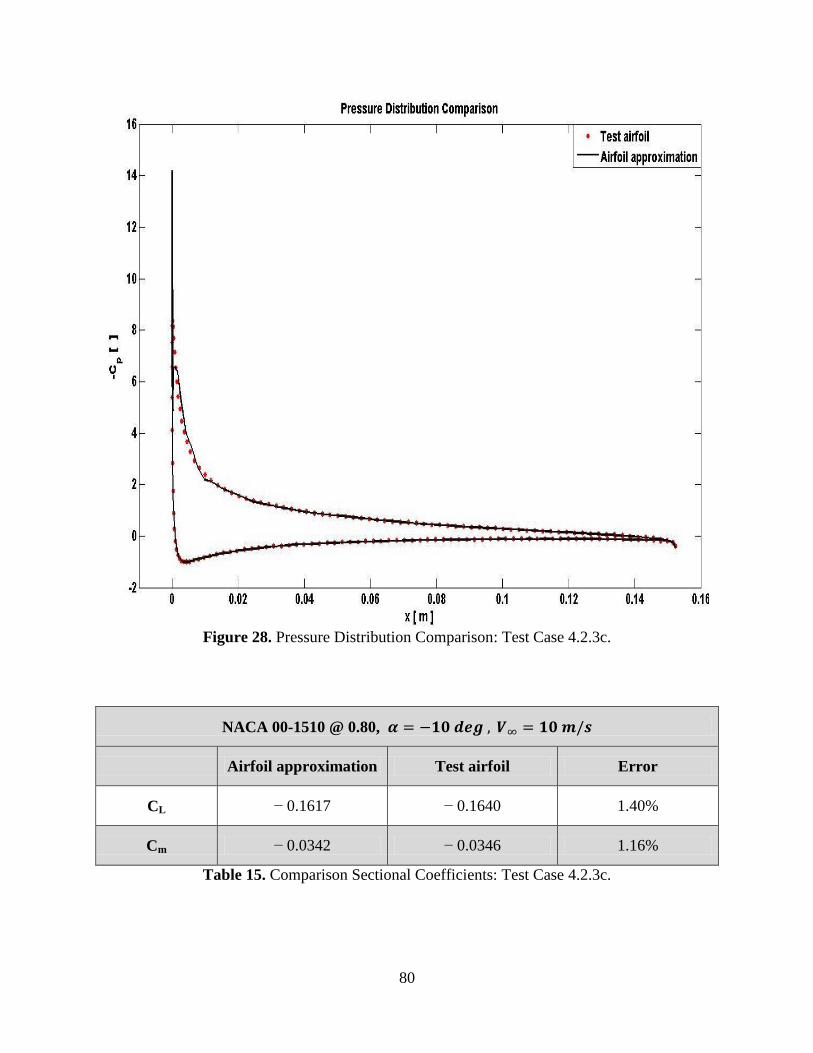
80

NACA 00-1510 @ 0.80,


CL − 0.1617 − 0.1640 1.40%

Cm − 0.0342 − 0.0346 1.16%

Table 15. Comparison Sectional Coefficients: Test Case 4.2.3c.

Figure 28. Pressure Distribution Comparison: Test Case 4.2.3c.

81

Examination of Fig. 28 and Table 15 show that this airfoil approximation produced the best

results of the three test cases. The spike near the leading edge is still present in the pressure

distribution, but this is once again a single outlying value. The lift and moment coefficients

produced very accurate results, with approximation error less than 2 percent for both

coefficients.

These three test cases demonstrate that the AHS/ANN system has the ability to

approximate different airfoil shapes at various angles of attack, providing the shape is contained

within the domain of the training data set. Examining the results, it can be seen that Test Case

4.2.3a produced the highest errors of the aerodynamic properties considered. One possible reason

for this is because the airfoil in said test case was analyzed at zero angle of attack, causing the

flow to contact the leading edge area that tends to be relatively sharp from the leading edge

recovery process, thus inducing more error.

4.3 AHS/ANN and Aerodynamic Formulation Comparison

The first section of this chapter verifies that the aerodynamic formulation is capable of

determining the aerodynamic loads of a camber-deformed airfoil. Similarly, the second section

shows that the AHS/ANN system is capable of producing a cambered-deformed airfoil shape

approximation that demonstrates similar aerodynamic properties as those of test airfoil. The

accuracy of each of these methods was analyzed in comparison to test data obtained from XFoil

analysis. To further examine the accuracy of camber shapes predicted by the AHS/ANN system,

test cases with the same airfoil shape and flow properties are analyzed by both the aerodynamic

formulation and the AHS/ANN system, and the results are compared.

82

4.3.1 Test Case 4.3a – NACA 3310

The first test airfoil examined is a NACA 3310 at zero angle of attack and the design

flow velocity of the AHS/ANN system ( The mean camber line of the test

airfoil was analyzed using the aerodynamic formulation, and the test airfoil shape was then

approximated using the AHS/ANN system. The airfoil approximation and the test airfoil were

each input to XFoil and the aerodynamic properties were calculated for comparison. The

resulting section lift and moment coefficients as determined by the aerodynamic formulation, as

well as those of the AHS/ANN airfoil approximation and test airfoil, are given in Table 16.

NACA 3310,

Formulation XFoil AHS/ANN

0.3275 0.3494 0.3724

− 0.0688 − 0.0693 − 0.0750

Table 16. Comparison of Sectional Coefficients: Test Case 4.3a.

It can be seen that the section lift and moment coefficients were reasonably accurate with respect

to the XFoil results. To further analyze the accuracy of these results, the coefficient differences

of each method were calculated with the respect to both the XFoil data and the results from the

other method, as shown in Table 17.

NACA 3310,

Formulation - XFoil AHS/ANN - XFoil AHS/ANN -

Formulation

6.27 % 6.58 % 12.06 %

0.70 % 8.23 % 8.24 %

Table 17. Approximation Differences: Test Case 4.3a.

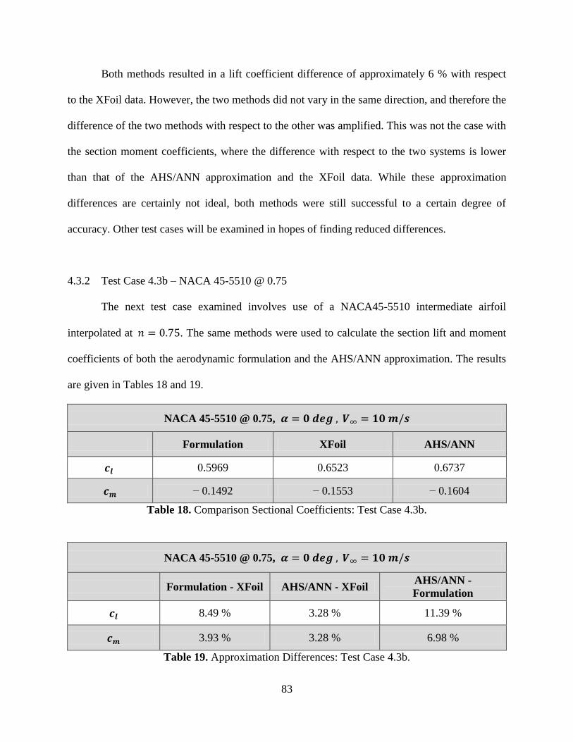
83

Both methods resulted in a lift coefficient difference of approximately 6 % with respect

to the XFoil data. However, the two methods did not vary in the same direction, and therefore the

difference of the two methods with respect to the other was amplified. This was not the case with

the section moment coefficients, where the difference with respect to the two systems is lower

than that of the AHS/ANN approximation and the XFoil data. While these approximation

differences are certainly not ideal, both methods were still successful to a certain degree of

accuracy. Other test cases will be examined in hopes of finding reduced differences.

4.3.2 Test Case 4.3b – NACA 45-5510 @ 0.75

The next test case examined involves use of a NACA45-5510 intermediate airfoil

interpolated at . The same methods were used to calculate the section lift and moment

coefficients of both the aerodynamic formulation and the AHS/ANN approximation. The results

are given in Tables 18 and 19.

NACA 45-5510 @ 0.75,


0.5969 0.6523 0.6737

− 0.1492 − 0.1553 − 0.1604

Table 18. Comparison Sectional Coefficients: Test Case 4.3b.

NACA 45-5510 @ 0.75,


Formulation

8.49 % 3.28 % 11.39 %

3.93 % 3.28 % 6.98 %

Table 19. Approximation Differences: Test Case 4.3b.

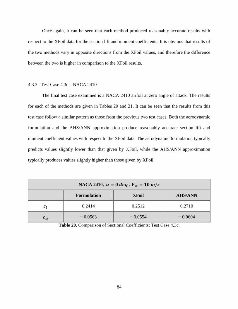
84

Once again, it can be seen that each method produced reasonably accurate results with

respect to the XFoil data for the section lift and moment coefficients. It is obvious that results of

the two methods vary in opposite directions from the XFoil values, and therefore the difference

between the two is higher in comparison to the XFoil results.

4.3.3 Test Case 4.3c – NACA 2410

The final test case examined is a NACA 2410 airfoil at zero angle of attack. The results

for each of the methods are given in Tables 20 and 21. It can be seen that the results from this

test case follow a similar pattern as those from the previous two test cases. Both the aerodynamic

formulation and the AHS/ANN approximation produce reasonably accurate section lift and

moment coefficient values with respect to the XFoil data. The aerodynamic formulation typically

predicts values slightly lower than that given by XFoil, while the AHS/ANN approximation

typically produces values slightly higher than those given by XFoil.

NACA 2410,


0.2414 0.2512 0.2710

− 0.0563 − 0.0554 − 0.0604

Table 20. Comparison of Sectional Coefficients: Test Case 4.3c.

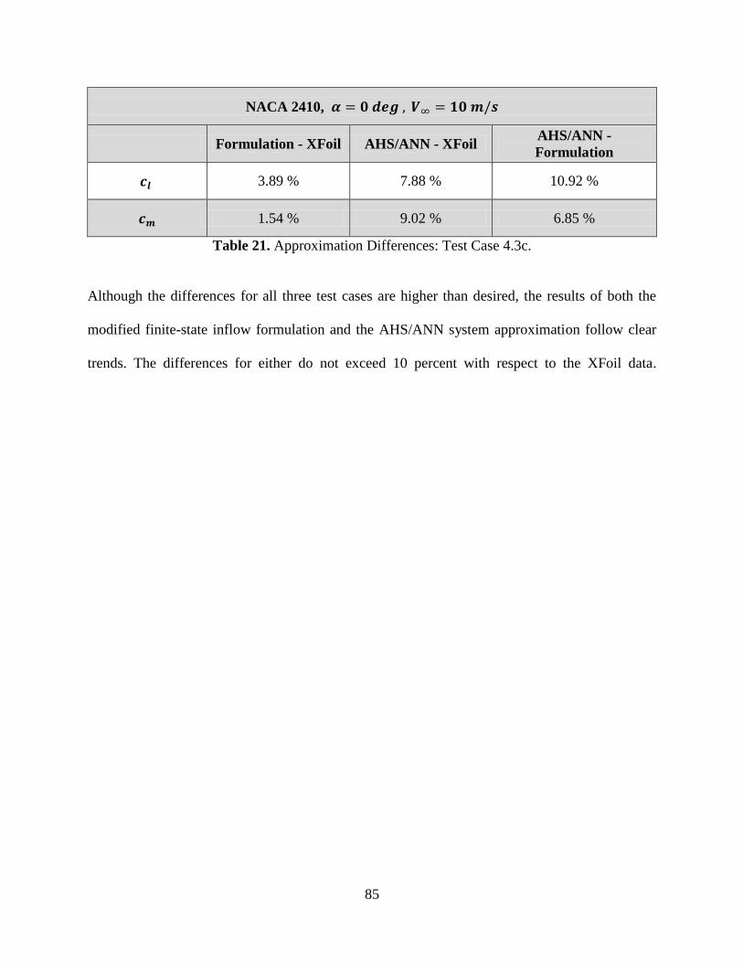
85

NACA 2410,


Formulation

3.89 % 7.88 % 10.92 %

1.54 % 9.02 % 6.85 %

Table 21. Approximation Differences: Test Case 4.3c.

Although the differences for all three test cases are higher than desired, the results of both the

modified finite-state inflow formulation and the AHS/ANN system approximation follow clear

trends. The differences for either do not exceed 10 percent with respect to the XFoil data.

86

CHAPTER 5

CONCLUSIONS AND DISCUSSION

5.1 Conclusions

This thesis presented a two-dimensional, finite-state aerodynamic formulation for

determining the aerodynamic loads acting on an airfoil with dynamic camber deformation. The

aerodynamic formulation was derived from a two-dimensional finite-state lift model for

determining the generalized forces acting on deformable airfoils, shown in Ref. [4]. This theory

was then extended to include higher-order elastic degrees of freedom such that an arbitrary

camber deformation of a fully-deformable airfoil can be modeled. This was accomplished by

using Legendre polynomials to represent a general camber deformation and performing Glauert

expansions on all necessary variables in the original formulation.

Multiple test cases were examined to verify the validity of the modified finite-state

inflow formulation. Although the modified aerodynamic formulation is capable of accounting for

rigid-body airfoil motions and unsteady aerodynamic effects, it was desired to use the

aerodynamic loads as determined by the formulation as a means of validating the approximation

approach of the AHS/ANN system, which is XFoil based. Thus, the flow was defined to be

quasi-steady in each test case.

The first test case examined a camber deformed airfoil in the simplest manner possible.

The thin-airfoil was modeled as the mean camber line of a NACA 4-digit airfoil, rigid-body

motions were neglected, and the free-stream flow was defined to be purely horizontal. Also,

87

elastic effects of the airfoil were ignored by modeling the airfoil as a rigid-body with constant

camber deformation. The section lift and moment coefficients were then calculated and

compared to the XFoil results of the same airfoil.

Next, a similar system setup was modeled, and an elastic degree of freedom was added to

the system by implementing camber actuation throughout a specified time interval. The camber

shape, aerodynamic loads, and sectional coefficients were calculated and tracked throughout the

actuation process by representing all airfoil motions as quasi-steady. In other words, the camber

deformation and aerodynamic loads were determined independently at each time interval such

that no dynamic, unsteady effects were present. The results were then once again compared to

those from XFoil to determine the accuracy. However, the numerical studies did not consider the

unsteadiness of the aerodynamic loads resulting from the camber actuation.

In addition, a process by which to approximate the shape of a cambered airfoil with

various deformations was developed. A series of NACA 4-digit airfoil shapes were used to

simulate camber actuation, and XFoil was used to generate the neural network training data at a

design free-stream velocity and a range of angles of attack. The XFoil data included local

velocity readings along the airfoil surface, which effectively simulates measurements from

artificial hair sensors. The local velocity measurements and their corresponding coordinates were

fed to a neural network in order to form a nodal approximation of the airfoil shape. The overall

airfoil shape was then recovered from the nodal approximation by curve-fitting, and the final

airfoil approximation was input to XFoil to verify the accuracy of the approximation.

Finally, numerous test cases were performed in which a camber-deformed airfoil was

analyzed using both the aerodynamic formulation and the AHS/ANN system approximation

approach. The section lift and moment coefficients were calculated for both methods and

88

compared to one another, along with the section lift and moment coefficients of the test airfoil as

determined by XFoil. The differences of all three were then compared to one another to verify

the approximation approach. It was found that both methods agree to one another with an

average percent difference. The results proved to contain higher differences than desired in some

cases, but both methods produced results that were reasonably accurate in comparison to the

XFoil results. The results of both approaches followed the same general trend for each of the test

cases, with the aerodynamic formulation generally producing section coefficients lower than that

of the XFoil analysis, and the AHS/ANN system producing section coefficients slightly higher

than the XFoil results. Also, the lift coefficients were found to contain significantly higher

difference values than the moment coefficients in both approaches.

5.2 Contributions

Overall, the majority of the goals that were set at the beginning of this work were

ultimately achieved. The finite-state inflow theory was successfully modeled to include higher-

order finite-state modes, which are used to represent a camber deformation of a fully-deformable

airfoil. Also, this formulation was implemented into a MATLAB code to account for time-

dependent camber actuation, allowing the aerodynamic loads to be tracked throughout an

actuation process in a quasi-steady manner. The theoretical approach of the aerodynamic

formulation was verified through multiple test cases, two of which are outlined in section (4.1).

Also, a neural network based approximation approach using artificial hair sensors was

successfully expanded upon to enable airfoil shape and flow state awareness. The approximation

approach was first verified through numerous test cases by comparing various aerodynamic

properties of the AHS/ANN airfoil approximation to those of the test airfoil, as determined by

89

XFoil. Additional test cases were examined in which the same test airfoil was analyzed by both

the theoretical aerodynamic formulation and XFoil analysis of the AHS/ANN airfoil shape

approximation. Since cambered airfoils are the subject of study in this work, the sectional

moment about the aerodynamic center is known to be the most important property in analyzing

the accuracy of each approach. There is also known to be some error in the XFoil analysis, and

therefore the results produced from this flow solver should not be interpreted as the absolutely

correct values.

5.3 Future Work

There are numerous studies that can be examined in the future to improve upon the

developments and findings of this thesis. The main priority moving forward will be to improve

upon the accuracy of both the theoretical aerodynamic formulation and the AHS/ANN system

approximation. One approach to improve upon the accuracy and efficiency of the AHS/ANN

system is to use multiple neural networks for the nodal approximation, which can in turn allow

for more overall output nodes and decrease computational time. Additionally, the AHS/ANN

training data can be expanded to include a range of free-stream velocities, as opposed to only a

single one. Ultimately, the AHS/ANN system will be tested in future studies by using actual

AHS measurement data, as opposed to simulated measurements from XFoil.

The aerodynamic formulation can potentially be improved upon by examining test cases

that include dynamic, unsteady aerodynamic properties. Considering such effects will likely

improve the accuracy of the approximation significantly. After improving upon both methods,

the entire system can be implemented into a closed-loop feedback control system, allowing for

the system to be used in three-dimensional aircraft control studies.

90

REFERENCES

(1) E. Stanewsky. “Aerodynamic Benefits of Adaptive Wing Technology”. Aerospace

Science and Technology , Vol. 4, No. 7, 2000, pp. 439-452.

(2) A. Rodriguez. “Morphing Aircraft Technology Survey”. 45th AIAA Aerospace Sciences

Meeting and Exhibit. American Institute of Aeronautics and Astronautics.

(3) C.M. Wang, C. Tung, and K.W. McAlister. “A Numerical Study of Airfoil Deformation

on Dynamic Stall”. 12th

AIAA Applied Aerodynamics Conference, Colorado Springs,

CO, June 20-22, 2994. Paper No. AIAA 94-1994.

(4) D. Peters and M. Johnson. “Finite-state Airloads for Deformable Airfoils on Fixed and

Rotating Wings”. Aeroelasticity and Fluid/Structures Interaction Problems, a Mini-

Symposium. ASME Winter Annual Meeting, Chicago, IL, Nov. 6-11, 1994, AD - Vol.

44, pp. 1-28.

(5) K. Magar, G. W. Reich, M. Rickey, B. Smyers, and R. Beblo. “Aerodynamic

Characteristics Prediction Via Artificial Hair Sensor and Feedforward Neural Network”.

ASME 2015 Conference on Smart Materials, Adaptive Structures and Intelligent

Systems,2015. SMASIS2015, September 21-23, 2015, Denver, CO, USA.

(6) J. Parcell, N. Aydemir, H. Devaraj, J. Travas-Sejdic, D.E. Williams, and K.C. Aw. “A

Novel Air Flow Sensor From Printed PEDOT Micro-Hairs”, 2013. IOP Publishing Ltd.,

Smart Materials and Structures, Vol. 22, No. 11.

(7) J. Tao and X. Yu. “Hair Flow Sensors: From Bio-Inspiration To Bio-Mimicking—A

Review”, 2012. IOP Publishing Ltd., Smart Materials and Structures, Vol. 21, No. 11.

(8) S. Sterbing-D’Angelo, M. Chadha, C. Chiu, B. Falk, W. Xian, J. Barcelo, J.M. Zook and

C.F. Moss. “Bat Wing Sensors Support Flight Control”, 2011. Proceedings of the

National Academy of Sciences of the United States of America, Vol. 108, No. 27.

(9) B. Dickinson, J. Baur, and G. W. Reich. “Embedded Sensors for Autonomous Air

Systems”. LRIR 09RW10COR. Air Force Research Lab Eglin AFB, FL, Munitions

Directorate, 2012.

(10) M. Hagan, H. Demuth, M. Beale, and O. De Jesus. Neural Network Design, 2nd

edition.

Boston: Pws Pub., 1996.

91

(11) K. Hornik, M Stinchcombe, and H. White. “Multilayer Feedforward Neural Networks

Are Universal Approximators”. Neural Networks 2, Vol. 5 (1989): pp. 359-366.

(12) D. Peters, S. Karunamoorthy, and W.M. Cao. “Finite State Induced Flow Models Part I:

Two-Dimensional Thin Airfoil”. Journal of Aircraft, Vol. 32, No. 2: pp. 313-322.

(13) W. Su. “Dynamic Aeroelastic Response of Highly Flexible Aircraft with Wing Camber

Deformations”, 2015. 56th AIAA/ASCE/AHS/ASC Structures, Structural Dynamics, and

Materials Conference. American Institute of Aeronautics and Astronautics.

(14) J. Murua, R. Palacios, and J. Peiro. “Camber Effects In The Dynamic Aeroelasticity Of

Compliant Airfoils”, 2010. Journal of Fluids and Structures, Vol. 26, No. 4: 527-543.

estimation of morphing airfoil shapes and...

Documents