Estimation of passive microseismic event location using random sampling based curve fittingLijun Zhu∗, Yang Zhao†, Weichang Li†, Entao Liu∗, James H. McClellan∗, Zefeng Li‡, and Zhigang Peng‡∗ Center for Energy and Geo Processing at Georgia Tech and King Fahd University of Petroleum and Minerals† Aramco Services Company: Aramco Research Center—Houston‡ School of Earth and Atmospheric Sciences, Georgia Institute of Technology

SUMMARY

Characterization of microseismic activities has become a use-ful tool for both hydraulic fracturing and seismic hazard mon-itoring. The microseismic data received by a sensor array typ-ically have relative weak signals in the presence of noise andinterference. Estimation of microseismic event locations usingsuch noisy data is always a major challenge of passive moni-toring, especially for a surface array.To overcome a large number of false picks due to backgroundnoise, a random sampling method is applied to classify pickedarrival times into event and nonevent clusters. By isolatingfalse picks into nonevent clusters, picks corresponding to seis-mic events are highlighted which can then be used to estimatethe event location using a background velocity model. A syn-thetic study shows this method is robust even in the presenceof significant lateral and vertical velocity variations using theMarmousi model. Field data of a 5200-element dense arrayin Long Beach, CA was utilized to evaluate the estimation ofmicroseismic event locations.

INTRODUCTION

Locations of microseismic events provide valuable informa-tion for reservoir monitoring during hydraulic fracturing (Dun-can, 2005). Identifying microseismic events where severe back-ground noise is present is always a challenging task. Vesnaveret al. (2011) combined both surface and borehole arrays to mit-igate the noise challenge. Even though microseismic eventswere successfully detected by this array setup, event localiza-tion was not feasible due to the overwhelming noise observedon both arrays (Vesnaver et al., 2012; Menanno et al., 2013).

Since the velocity model is generally not perfectly known dur-ing microseismic monitoring, travel-time based location meth-ods are applied under an initial effective homogeneous mediumassumption (Grechka and Zhao, 2012). Blias and Grechka(2013) gives an analytic solution to jointly estimate the eventlocations and an effective velocity model for microseismic ap-plications by fitting a parabola curve to travel time differencesbetween P-wave and S-wave arrivals. When only a P-wavephase is available, a hyperbola can be used instead to modelthe moveout curve on the monitoring array (Dix, 1955). How-ever, due to background noise, a large number of false pickswill contaminate picked arrival times and make such curve fit-ting results unreliable.

To overcome this challenge and eliminate false picks, Zhu et al.(2016) proposed Random-sampling-based Arrival Time EventClustering (RATEC) — a method to find the most reliable move-out curve. The moveout curve is isolated from false picks by

repeatedly trying different hypothesized curves and finding thebest curve that agrees with the largest number of picked arrivaltimes. In this study, we show successful application of RATECon a dense surface array setup for earthquake monitoring (Zhuet al., 2017), as well as synthetic examples with P- and S-wavephases and complex velocity models.

METHOD

RANdom SAmpling Consensus (RANSAC)Random sampling consensus was first proposed by Fischlerand Bolles (1981) and then improved by many others (Stew-art, 1995; Torr and Zisserman, 2000; Chum and Matas, 2002;Tordoff and Murray, 2005; Chum and Matas, 2005). Despitemany variations and adaptations of random sampling (Choiet al., 2009), there are essentially two steps per iteration whichare repeated many times to determine the best fit to the data:

• Hypothesize: A minimal sample subset (MinSet, de-noted as Ωk

M) is randomly selected from the datasetand the unique model parameters (pk) are computedfor Ωk

M.

• Test: Elements in the dataset (ΩD) are evaluated to de-termine which ones can be labeled as inliers, i.e., con-sistent with the hypothesized model in the sense thatthe distance from the model’s moveout curve is lessthan some prescribed value (δ ). The set of all such in-liers is called a consensus set (ConSet, denoted as Ωk

C).

Note that ΩkM ⊂ Ωk

C ⊂ ΩD. A set ΩkM consists of only the

minimal number of samples required to uniquely determinea model, e.g., two samples for a line and three for a circle.The more elements in Ωk

C, the better the model we have ob-tained for the kth hypothesis. Based on the fitted hyperbolicmodel, the picked arrival times are, in effect, clustered intoevent groups and nonevent groups. Such clustering not onlyseparates picked arrival times into different phases (e.g., P-wave and S-wave phases), but also improves the accuracy oflocalization results by eliminating false picks due to noise.

Each RANSAC iteration requires very little computation andthere exists a unique solution for each chosen MinSet. In thisway, we can afford to use a large number of iterations to dis-cover a consistent model. The number of iterations N to guar-antee that at least one ΩM will only contain true picks withprobability p is

N =log(1− p)

log(1−um), (1)

where u is the fraction of all picks that are close to a hyperbola,and m is the size of a MinSet, which is 5 for a hyperbola and

© 2017 SEG SEG International Exposition and 87th Annual Meeting

Page 2791

Dow

nloa

ded

09/0

5/17

to 1

30.2

07.6

7.81

. Red

istr

ibut

ion

subj

ect t

o SE

G li

cens

e or

cop

yrig

ht; s

ee T

erm

s of

Use

at h

ttp://

libra

ry.s

eg.o

rg/

Passive microseismics by RATEC

RANSAC iterations Terminate Iteration

PerturbedSampling

BuildMinSet

EstimateParameter

ParametricModel

ConstructConSet

D kM

pk

kC

C

Estimate#Iter Max

TerminateCondition

Yes

No

ChooseConSet

C

p

EstimateInlier Ratio

up

N

Nmax Nmin

Figure 1: Complete workflow of proposed random sampling scheme.

9 for a hyperboloid. For example, when u = 0.5 and m = 5,we can guarantee a 99% chance of finding an outlier-free ΩM(p = 0.99), if we run N = 145 iterations.

The overall process of RATEC is summarized in a flow chartin Figure 1. After the kth iteration, the current best ConSet Ω∗Cis updated with the kth ConSet if Ωk

C has more inliers. ThenΩ∗C is used to estimate the current best inlier ratio u∗. Basedon Equation (1), the number of iterations required, N, can beupdated (Tordoff and Murray, 2005). The current N is alsocompared against preset minimum and maximum values Nminand Nmax. Once the termination condition is satisfied, the bestConSet Ω∗C and model parameter p∗ are returned; otherwise,the iteration loop will continue.

Parameter estimation for moveout curveThe proposed method uses a quadratic model to estimate theparameters of a hyperbolic curve, which takes the followingform:

P(x,y;p) = ax2 +bxy+ cy2 +dx+ ey+ f = 0, (2)

where p has six real elements (a, · · · , f ). There are actuallyonly five free parameters, since one of the nonzero elementscan be always normalized to 1. When the determinant

∆1 = 4

∣∣∣∣∣ a b/2 d/2b/2 c e/2d/2 e/2 f

∣∣∣∣∣ (3)

is nonzero (∆1 6= 0), Equation (2) defines a non-degenerateconic section. To verify that it is a hyperbola, we must alsocheck a second determinant

∆2 = 4∣∣∣ a b/2

b/2 c

∣∣∣= b2−4ac. (4)

When ∆2 > 0, Equation (2) defines a hyperbola.

Given n arrival time picks, (xi,yi) for i = 1, . . . ,n, we form an×6 data matrix Dn and a 6×1 coefficient vector p, such thatDnp is the model P(x,y;p) evaluated at the time picks. Withmeasurement error, there is a nonzero residual r, i.e., x2

1 x1y1 y21 x1 y1 1

......

......

......

x2n xnyn y2

n xn yn 1

abcdef

=

r1...

rn

⇔ Dnp = r.

(5)

If all picks in ΩM are true picks, the residual term r is negli-gible. Then we solve the linear system D5p = 000, which findsthe null space of D5. From the singular value decomposition(SVD) of D5, it is easy to see that the last right singular vec-tor v6 ∈ null(D5). To further stabilize the algorithm, a randomperturbation is added to yi when MinSets are formed.

Extension to 2-D surface arraysThis fitting method can be easily extended to surface arrays bychanging the underlying hyperbolic curve model to a hyper-boloid surface model. Similar to Equation (2), a hyperboloidsurface can be defined using a quadratic equation in (x,y,z)that takes the following general form:

P(x,y,z;p) = [x y z]

[a b/2 d/2

b/2 c e/2d/2 e/2 g

][ xyz

]+[g h i]

[ xyz

]+ j = 0

(6)

Using (6), the RANSAC framework can be adapted to hy-perboloid surface fitting by finding the parameter vector p =[a,b,c,d,e, f ,g,h, i, j] in a 10-dimensional space. Althoughthis is a somewhat larger parameter space for the MinSets, itadds very little burden to the search process because RATECstill searches the n time picks using models formed from therandomly chosen MinSets which now have 9 elements.

Event location through moveout curveVarious location methods based on travel time can be used onthe time picks in the event cluster after RATEC is applied. Be-low, we offer one simple location estimation by refitting themoveout curves based on an effective homogeneous media as-sumption. We choose the trust region method (Berghen, 2004)over the least squares method for refitting due to its robust-ness in the presence of general background noise. UnpackingEquation (2), the event location can be recovered from the hy-perbola coefficients as follows:

x0 =−d2a

and z0 =

√fa− d2

4a2 −ce2

4ac2 . (7)

where x0 is the event horizontal offset and z0 is the event depth.

© 2017 SEG SEG International Exposition and 87th Annual Meeting

Page 2792

Dow

nloa

ded

09/0

5/17

to 1

30.2

07.6

7.81

. Red

istr

ibut

ion

subj

ect t

o SE

G li

cens

e or

cop

yrig

ht; s

ee T

erm

s of

Use

at h

ttp://

libra

ry.s

eg.o

rg/

Passive microseismics by RATEC

SYNTHETIC DATA EXAMPLE

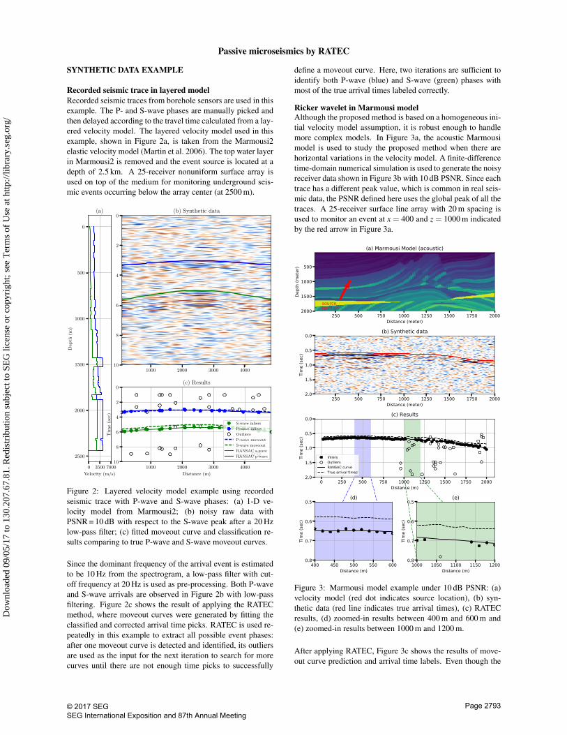
Recorded seismic trace in layered modelRecorded seismic traces from borehole sensors are used in thisexample. The P- and S-wave phases are manually picked andthen delayed according to the travel time calculated from a lay-ered velocity model. The layered velocity model used in thisexample, shown in Figure 2a, is taken from the Marmousi2elastic velocity model (Martin et al. 2006). The top water layerin Marmousi2 is removed and the event source is located at adepth of 2.5 km. A 25-receiver nonuniform surface array isused on top of the medium for monitoring underground seis-mic events occurring below the array center (at 2500 m).

0 3500 7000

Velocity (m/s)

0

500

1000

1500

2000

2500

Dep

th(m

)

(a)

1000 2000 3000 4000

0

2

4

6

8

10

(b) Synthetic data

1000 2000 3000 4000

Distance (m)

0

2

4

6

8

10

Tim

e(s

ec)

(c) Results

S-wave inliers

P-wave inliers

Outliers

P-wave moveout

S-wave moveout

RANSAC s-wave

RANSAC p-wave

Figure 2: Layered velocity model example using recordedseismic trace with P-wave and S-wave phases: (a) 1-D ve-locity model from Marmousi2; (b) noisy raw data withPSNR = 10 dB with respect to the S-wave peak after a 20 Hzlow-pass filter; (c) fitted moveout curve and classification re-sults comparing to true P-wave and S-wave moveout curves.

Since the dominant frequency of the arrival event is estimatedto be 10 Hz from the spectrogram, a low-pass filter with cut-off frequency at 20 Hz is used as pre-processing. Both P-waveand S-wave arrivals are observed in Figure 2b with low-passfiltering. Figure 2c shows the result of applying the RATECmethod, where moveout curves were generated by fitting theclassified and corrected arrival time picks. RATEC is used re-peatedly in this example to extract all possible event phases:after one moveout curve is detected and identified, its outliersare used as the input for the next iteration to search for morecurves until there are not enough time picks to successfully

define a moveout curve. Here, two iterations are sufficient toidentify both P-wave (blue) and S-wave (green) phases withmost of the true arrival times labeled correctly.

Ricker wavelet in Marmousi modelAlthough the proposed method is based on a homogeneous ini-tial velocity model assumption, it is robust enough to handlemore complex models. In Figure 3a, the acoustic Marmousimodel is used to study the proposed method when there arehorizontal variations in the velocity model. A finite-differencetime-domain numerical simulation is used to generate the noisyreceiver data shown in Figure 3b with 10 dB PSNR. Since eachtrace has a different peak value, which is common in real seis-mic data, the PSNR defined here uses the global peak of all thetraces. A 25-receiver surface line array with 20 m spacing isused to monitor an event at x = 400 and z = 1000 m indicatedby the red arrow in Figure 3a.

250 500 750 1000 1250 1500 1750 2000Distance (meter)

500

1000

1500

2000

Dept

h (m

eter

)sourcelocation

(a) Marmousi Model (acoustic)

250 500 750 1000 1250 1500 1750 2000Distance (meter)

0.0

0.5

1.0

1.5

2.0

Tim

e (s

ec)

(b) Synthetic data

0 250 500 750 1000 1250 1500 1750 2000Distance (m)

0.0

0.5

1.0

1.5

2.0

Tim

e (s

ec)

(c) Results

InliersOutliersRANSAC curveTrue arrival times

400 450 500 550 600Distance (m)

0.5

0.6

0.7

0.8

Tim

e (s

ec)

(d)

1000 1050 1100 1150 1200Distance (m)

0.5

0.6

0.7

0.8

Tim

e (s

ec)

(e)

Figure 3: Marmousi model example under 10 dB PSNR: (a)velocity model (red dot indicates source location), (b) syn-thetic data (red line indicates true arrival times), (c) RATECresults, (d) zoomed-in results between 400 m and 600 m and(e) zoomed-in results between 1000 m and 1200 m.

After applying RATEC, Figure 3c shows the results of move-out curve prediction and arrival time labels. Even though the

© 2017 SEG SEG International Exposition and 87th Annual Meeting

Page 2793

Dow

nloa

ded

09/0

5/17

to 1

30.2

07.6

7.81

. Red

istr

ibut

ion

subj

ect t

o SE

G li

cens

e or

cop

yrig

ht; s

ee T

erm

s of

Use

at h

ttp://

libra

ry.s

eg.o

rg/

Passive microseismics by RATEC

Figure 4: Top view of the sen-sor array with located event in-dicated by red star.

Figure 5: Snapshot ofthe seismic dataset attime t = 3020.00s; thevisible event lies insidethe red circle.

true moveout is not exactly a hyperbola, RATEC is able tolabel all the true arrival times within a small distance of themoveout curve. Zooming in around the horizontally layeredregion, good prediction and perfect labeling are observed inFigure 3d. Notice that there is a consistent offset betweenpicked and true arrival times due to the delay of STA/LTApickings (Zhao et al., 2008) used here. Figure 3e shows the re-sults in a more complex region where the SNR is worse. Eventhough many picks in that region are false picks, RATEC suc-cessfully eliminates most of the picks far away from the truemoveout curve and labels the true time picks correctly.

FIELD DATA EXAMPLE

The proposed method was also tested on a data set of 50 seccollected by the Long Beach nodal dense array (Inbal et al.,2016) in southern California which contains 5200 sensors. Thetop view of the sensor array is shown in Figure 4. Prior to ap-plying the RATEC scheme, no reliable location estimate can beobtained from the picked arrival times due to a large number offalse picks which are visible in Figure 6. Instead of STA/LTA,local similarity (Li and Peng, 2016) is used to improve the timepicking accuracy based on the stacked waveform similarity be-tween adjacent traces in a small area.

Using the clustered picks found by RATEC, this seismic eventis recognized as a surface event whose location is shown bymarking its epicenter with the red star in Figure 4. In orderto verify our result, we schematically show the correspondingclipped data amplitude snapshot on the sensor array in Figure5. The gray-scale of the dots indicates the clipped signal am-plitude on the corresponding sensor. The red circle in Figure 5confirms that in the inverted time and location using the clas-sified true picks, there is indeed a weak event that is barelyvisible in the raw array data. Moreover, the work log showsthat there is a surface source in the estimated area but the lo-cal earthquake catalog has no record of earthquakes during theevent time. In Figure 6 we show the time picking results thatcontain a large number of false picks. The best-fitted hyper-boloid surface from 3-D RATEC is shown as the red surface.On a laptop, RATEC takes just 31 sec to process 50 sec of data

Figure 6: 3-D view of the noisy picks () from the 2-D sensorarray. Fitted surface obtained via RATEC highlighted in red.

which is sufficient for real-time processing.

CONCLUSION

In this paper, we reformulated the arrival time picking probleminto a model fitting framework and extended the RANSAC-based curve fitting and surface fitting methods to classify pickedarrival times. The effectiveness and robustness of the proposedmethod are validated by tests on both synthetic and real datasets. The localization result is significantly improved whenRATEC eliminates false picks from the data set. In the 2Dsurface array example on real microseismic data, an accuratehypocenter is successfully inverted.

ACKNOWLEDGEMENTS

The seismic data analyzed in this study are owned by SignalHill Petroleum, Inc. and acquired by NodalSeismic LLC. Wethank NodalSeismic LLC for making the one-week data avail-able in this study. This work is supported by the Center forEnergy and Geo Processing (CeGP) at Georgia Tech and byKing Fahd University of Petroleum and Minerals. Zefeng Liand Zhigang Peng are supported by National Science Founda-tion grant EAR-1551022.

© 2017 SEG SEG International Exposition and 87th Annual Meeting

Page 2794

Dow

nloa

ded

09/0

5/17

to 1

30.2

07.6

7.81

. Red

istr

ibut

ion

subj

ect t

o SE

G li

cens

e or

cop

yrig

ht; s

ee T

erm

s of

Use

at h

ttp://

libra

ry.s

eg.o

rg/

EDITED REFERENCES

Note: This reference list is a copyedited version of the reference list submitted by the author. Reference lists for the 2017

SEG Technical Program Expanded Abstracts have been copyedited so that references provided with the online

metadata for each paper will achieve a high degree of linking to cited sources that appear on the Web.

REFERENCES

Berghen, F. V., 2004, Condor: A constrained, non-linear, derivative-free parallel optimizer for

continuous, high computing load, noisy objective functions: These de doctorat, Université Libre

de Bruxelles.

Blias, E., and V. Grechka, 2013, Analytic solutions to the joint estimation of microseismic event locations

and effective velocity model: Geophysics, 78, no. 3, KS51–KS61,

https://doi.org/10.1190/geo2012-0517.1.

Choi, S., T. Kim, and W. Yu, 2009, Performance evaluation of RANSAC family: Journal of Computer

Vision, 24, 271–300, https://doi.org/10.5244/C.23.81.

Chum, O., and J. Matas, 2002, Randomized RANSAC with T(d, d) test: Proceedings of the British

Machine Vision Conference, 448–457, https://doi.org/10.5244/C.16.43.

Chum, O., and J. Matas, 2005, Matching with PROSAC-progressive sample consensus: 2005 IEEE

Computer Society Conference on Computer Vision and Pattern Recognition (CVPR’05), IEEE,

220–226, https://doi.org/10.1109/CVPR.2005.221.

Dix, C. H., 1955, Seismic velocities from surface measurements: Geophysics, 20, 68–86,

https://doi.org/10.1190/1.1438126.

Duncan, P. M., 2005, Is there a future for passive seismic?: First Break, 23.

Fischler, M. A., and R. C. Bolles, 1981, Random sample consensus: A paradigm for model fitting with

applications to image analysis and automated cartography: Communications of the ACM, 24,

381–395, https://doi.org/10.1145/358669.358692.

Grechka, V., and Y. Zhao, 2012, Microseismic interferometry: The Leading Edge, 31, 1478–1483,

https://doi.org/10.1190/tle31121478.1.

Inbal, A., J. P. Ampuero, and R. W. Clayton, 2016, Localized seismic deformation in the upper mantle

revealed by dense seismic arrays: Science, 354, 88–92, https://doi.org/10.1126/science.aaf1370.

Li, Z., and Z. Peng, 2016, Automatic detection and classification of seismic events: Seismological

Research Letters, 87, 501.

Martin, G. S., R. Wiley, and K. J. Marfurt, 2006, Marmousi2: An elastic upgrade for Marmousi: The

Leading Edge, 25, 156–166, https://doi.org/10.1190/1.2172306.

Menanno, G., A. Vesnaver, and M. Jervis, 2013, Borehole receiver orientation using a 3D velocity model:

Geophysical Prospecting, 61, 215–230, https://doi.org/10.1111/j.1365-2478.2012.01106.x.

Stewart, C. V., 1995, MINPRAN: A new robust estimator for computer vision: IEEE Transactions on

Pattern Analysis and Machine Intelligence, 17, 925–938, https://doi.org/10.1109/34.464558.

Tordoff, B. J., and D. W. Murray, 2005, Guided-MLESAC: Faster image transform estimation by using

matching priors: IEEE Transactions on Pattern Analysis and Machine Intelligence, 27, 1523–

1535, https://doi.org/10.1109/TPAMI.2005.199.

Torr, P. H., and A. Zisserman, 2000, MLESAC: A new robust estimator with application to estimating

image geometry: Computer Vision and Image Understanding, 78, 138–156,

https://doi.org/10.1006/cviu.1999.0832.

Vesnaver, A., G. Menanno, S. I. Kaka, and M. Jervis, 2011, 3D polarization analysis of surface and

borehole microseismic data: 81th Annual International Meeting, SEG, Expanded Abstracts,

1663–1668, https://doi.org/10.1190/1.3627523.

Vesnaver, A., G. M. Menanno, and M. Jervis, 2012, Accuracy analysis for the hypocenter estimate in a

microseismic survey: Presented at the GEO 2012, EAGE.

© 2017 SEG SEG International Exposition and 87th Annual Meeting

Page 2795

Dow

nloa

ded

09/0

5/17

to 1

30.2

07.6

7.81

. Red

istr

ibut

ion

subj

ect t

o SE

G li

cens

e or

cop

yrig

ht; s

ee T

erm

s of

Use

at h

ttp://

libra

ry.s

eg.o

rg/

Zhao, Y., C. Tang, and J. A. Rial, 2008, A new approach for the automatic detection of shear-wave

splitting: M.S. thesis, The University Of North Carolina At Chapel Hill.

Zhu, L., Z. Li, Z. Peng, E. Liu, and J. H. McClellan, 2017, Weighted random sampling in seismic event

detection/location (WRASED): Applications to local, regional, and global seismic networks:

Annual Meeting Seismological Society of America, Seismological Research Letters, 88.

Zhu, L., E. Liu, and J. H. McClellan, 2016, An automatic arrival time picking method based on RANSAC

curve fitting: 78th Annual International Conference and Exhibition, EAGE, Extended Abstracts,

https://doi.org/10.3997/2214-4609.201601481.

© 2017 SEG SEG International Exposition and 87th Annual Meeting

Page 2796

Dow

nloa

ded

09/0

5/17

to 1

30.2

07.6

7.81

. Red

istr

ibut

ion

subj

ect t

o SE

G li

cens

e or

cop

yrig

ht; s

ee T

erm

s of

Use

at h

ttp://

libra

ry.s

eg.o

rg/