HAL Id: hal-00907484https://hal.inria.fr/hal-00907484v2

Submitted on 26 Nov 2013

HAL is a multi-disciplinary open accessarchive for the deposit and dissemination of sci-entific research documents, whether they are pub-lished or not. The documents may come fromteaching and research institutions in France orabroad, or from public or private research centers.

L’archive ouverte pluridisciplinaire HAL, estdestinée au dépôt et à la diffusion de documentsscientifiques de niveau recherche, publiés ou non,émanant des établissements d’enseignement et derecherche français ou étrangers, des laboratoirespublics ou privés.

Estimation of the caesium-137 source term from theFukushima Daiichi nuclear power plant using a

consistent joint assimilation of air concentration anddeposition observations

Victor Winiarek, Marc Bocquet, Nora Duhanyan, Yelva Roustan, OlivierSaunier, Anne Mathieu

To cite this version:Victor Winiarek, Marc Bocquet, Nora Duhanyan, Yelva Roustan, Olivier Saunier, et al.. Estimation ofthe caesium-137 source term from the Fukushima Daiichi nuclear power plant using a consistent jointassimilation of air concentration and deposition observations. Atmospheric environment, Elsevier,2014, 82, pp.268-279. �10.1016/j.atmosenv.2013.10.017�. �hal-00907484v2�

Estimation of the caesium-137 source term from the Fukushima Daiichi nuclearpower plant using a consistent joint assimilation of air concentration and

deposition observations

Victor Winiareka,b, Marc Bocqueta,b, Nora Duhanyana, Yelva Roustana, Olivier Saunierc, Anne Mathieuc

aUniversite Paris-Est, CEREA, joint laboratoryEcole des Ponts ParisTech and EDF R&D, Champs-sur-Marne, FrancebINRIA, Paris Rocquencourt research centre, France

cInstitut de Radioprotection et de Surete Nucleaire (IRSN), PRP-CRI, SESUC, BMTA, Fontenay-aux-Roses, 92262, France

Abstract

Inverse modelling techniques can be used to estimate the amount of radionuclides and the temporal profile of thesource term released in the atmosphere during the accident of the Fukushima Daiichi nuclear power plant in March2011. In Winiarek et al. (2012b), the lower bounds of the caesium-137 and iodine-131 source terms were estimatedwith such techniques, using activity concentration measurements. The importance of an objective assessment of priorerrors (the observation errors and the background errors) was emphasised for a reliable inversion. In such criticalcontext where the meteorological conditions can make the source term partly unobservable and where only a fewobservations are available, such prior estimation techniques are mandatory, the retrieved source term being verysensitive to this estimation.

We propose to extend the use of these techniques to the estimation of prior errors when assimilating observationsfrom several data sets. The aim is to compute an estimate of the caesium-137 source term jointly using all availabledata about this radionuclide, such as activity concentrations in the air, but also daily fallout measurements and totalcumulated fallout measurements. It is crucial to properly and simultaneously estimate the background errors andthe prior errors relative to each data set. A proper estimation of prior errors is also a necessary condition to reliablyestimate the a posteriori uncertainty of the estimated source term. Using such techniques, we retrieve a total releasedquantity of caesium-137 in the interval 11.6 − 19.3 PBq with an estimated standard deviation range of 15− 20%depending on the method and the data sets. The “blind” time intervals of the source term have also been stronglymitigated compared to the first estimations with only activity concentration data.

This article has been published in Atmospheric Environmentwith the reference:Winiarek, V., Bocquet, M., Duhanyan, N., Roustan, Y., Saunier, O., Mathieu, A., 2014. Estimation of the caesium-137source term from the Fukushima Daiichi nuclear power plant using a consistent joint assimilation of air concentrationand deposition observations.Atmos. Env.82. 268-279.

Keywords: Data assimilation, Atmospheric dispersion, Fukushima accident, Source estimation

1. Introduction

1.1. The Fukushima Daiichi accident

On March 11, 2011, 05:46 UTC, a magnitude 9.0(Mw) undersea megathrust earthquake occurred in thePacific Ocean and an extremely destructive tsunamihit the Pacific coast of Japan approximately one hourlater. These events caused the automatic shut-down of

Email address:bocquet@cerea.enpc.fr (Marc Bocquet)

4 power plants in Japan. Diesel backup power sys-tems should have sustained the reactors cooling process.In Fukushima Daiichi these backup devices were un-fortunately inoperative mainly because of the damagescaused by the tsunami.

The Fukushima Daiichi NPP has six nuclear reactors.At the time of the earthquake, reactor 4 had been de-fuelled and reactors 5 and 6 were in a cold shut-downfor planned maintenance.

In the hours that followed, the situation quickly be-

Preprint submitted to Atmospheric Environment November 26, 2013

came critical. Reactors 1, 2 and 3 experienced at leastpartial meltdown and hydrogen explosions. Addition-ally, fuel rods stored in pools in each reactor buildingbegan to overheat as water levels in the pools dropped.

All these events caused a massive discharge of ra-dioactive materials in the atmosphere. The total quan-tities of released radionuclides as well as the time evo-lution of these releases have to be estimated in order toassess the sanitary and environmental impact of the ac-cident.

Mathieu et al. (2012) used core inventories and in-situ data (pressure and temperature measurements in thereactors andγ-dose rates in the NPP) as well as firstavailable observations over Japan to build a source term,which was used in Korsakissok et al. (2013) to assessthe highγ-dose rates zones at a local scale. Chino et al.(2011) used a few activity concentration measurementsin the air to calibrate the magnitude of some identifiedreleases of131I and137Cs. Katata et al. (2012) and Ter-ada et al. (2012) updated these estimations as new datawere available. Stohl et al. (2012) performed an inversemodelling estimation using activity concentrations inthe air, as well as deposition data at a global scale toestimate the release of133Xe and137Cs. However theirestimation was shown to be quite sensitive to the priorinformation on the source used in the inversion. At thesame time, Winiarek et al. (2012b) proposed a methodto properly estimate the prior errors to perform inversemodelling using activity concentrations in the air. Theyapplied it to estimate the source terms of131I and137Cs.

1.2. Objectives and outlineIn Winiarek et al. (2012b) we emphasised the impor-

tance of a proper estimation of prior errors in the inversemodelling algorithm. We proposed new methods to esti-mate two hyper-parameters: the variance of observationerrors and the variance of background errors, assumingthat all observation errors have the same variance. Thisassumption is acceptable when using only one type ofdata in the algorithm. On the other hand the generallack of data in accidental situations stresses the need foralgorithms that would use all available data in the sameinversion. The first objective of this paper is to extendthe methods proposed in Winiarek et al. (2012b) to thesimultaneous estimation of prior errors when using dif-ferent data sets in the inversion. The second objectiveis to apply these methods to the challenging reconstruc-tion of the caesium-137 source term of the FukushimaDaiichi accident, as well as to obtain an objective un-certainty on this estimation.

In Section 2 we briefly recall the methodology for theinverse modelling of accidental releases of pollutants.

The algorithm is sensitive to the statistics of the errors sothat we propose methods based on the maximum like-lihood principle to estimate these errors. This generalmaximum likelihood scheme takes into account the pos-itivity of the source and the presence of several types ofdata.

In Section 3 we apply this new method to the re-construction of the atmospheric release of137Cs fromthe Fukushima Daiichi power plant. The inversions arecomputed using three data sets: activity concentrationsin the air, daily measurements of deposited materialand total cumulated deposition. The new source termsare discussed and compared to earlier estimations. Theposterior uncertainties of the retrieved sources are alsocomputed.

Results are summarised and conclusions are given inSection 4.

2. Methodology

2.1. Inverse modelling of accidental releases and esti-mation of errors

To reconstruct the source term of an accidental re-lease of a pollutant into the atmosphere, inverse mod-elling techniques are a powerful alternative to a trial anderror approach with direct numerical models, which isstill widely used in such situations. Inverse modellingtechniques can objectively estimate the source term us-ing the information content of an observation set anda numerical model that simulates the dispersion event.The atmospheric transport model (ATM), which is lin-ear in our case for gaseous and particulate matter, pro-vides the relationship between the source term and theobservation set through the source-receptor equation

µ = Hσ + ǫ , (1)

whereµ in Rd is the measurement vector,σ in R

N is thesource vector, andH is the Jacobian matrix of the trans-port model which incorporates the observation operatoras well. The vectorǫ in R

d, called the observation er-ror in this article, represents the instrumental errors, therepresentativeness errors and a fraction of model erroraltogether.

In an accidental context the number of observationsis very often limited. Specific meteorological condi-tions, like during the Fukushima accident, can alsolead to a weak observability of a part of the sourceterm. In these cases, the source-receptor relationshipdefined by Eq. (1) constitutes an ill-posed inverse prob-lem (Winiarek et al., 2011).

2

One solution to deal with the lack of constraints is toimplement parametric methods where the source to re-trieve is reduced to a very limited number of parameters.The inverse problem isde factoregularised and it canbe solved using different techniques, such as stochasticsampling techniques which allow to access the parame-ters posterior distributions (Delle Monache et al., 2008;Yee et al., 2008). Nevertheless if the true source doesnot match the parametric model, the inversion may failor yield a meaningless solution.

Another option is the use of non-parametric methodsto retrieve a general source field. This field can be dis-cretised, for example to match the model discretisation,but the number of variables remains large and may stillbe larger than the number of observations in the dataset. The non-parametric approach is robust and flexi-ble since no strong a priori assumptions are made onthe source but it has its own constraints. If Gaussianstatistics are assumed for observation errors, the inver-sion relies on the minimisation of the cost function

L(σ) =12

(µ −Hσ)T R−1 (µ −Hσ) , (2)

where R is the observation error covariance matrix:R = E

[

ǫǫT]

, whereǫ has been defined by Eq. (1). Onesimple choice is to neglect correlations between obser-vation errors and to takeR diagonal. If all the obser-vations are of the same type, one can even assume thatR = r2Id, r2 being the variance of the observation errors(Id is the identity matrix inR

d×d). With a low num-ber of observations and/or a poor observability of sev-eral source term parts, the minimisation of Eq. (2) givesinfinitely many solutions. One needs to regularise theinverse problem, usually by adding a Tikhonov term inthe cost function:

L(σ) =12

(µ −Hσ)T R−1 (µ −Hσ)

+12

(σ − σb)T B−1 (σ − σb) . (3)

The solution of the inverse problem is now unique,but two additional (vector and matrix) parameters havebeen introduced:σb is the first guess for the source (orbackground term) andB is the background error covari-ance matrix:B = E

[

(σ − σb) (σ − σb)T]

.In an accidental situation and particularly in the

Fukushima accident context, the choice ofσb = 0 isrelevant because (i) many of the parameters are likelyto be zero (ii) it guarantees an independent estimate (iii)it avoids the risk of aninversion crime, since most ofthe first guess built by physics models are eventuallycalibrated using early observations. One can refer to

Bocquet (2005); Davoine and Bocquet (2007); Winiareket al. (2012b) for extended discussions on this choice.

Still in an accidental context, off-diagonal terms inB are often negligible. For example theγ-dose mea-surements made in the Fukushima nuclear power plant(NPP) indicate that the source term is probably com-posed of uncorrelated events1. This is the reason whywe takeB = m2IN in this article.

As it was shown in the Chernobyl case in Davoineand Bocquet (2007) or in the Fukushima case inWiniarek et al. (2012b) or Stohl et al. (2012), the re-trieved source is very sensitive to the matricesR andB, hence to the two hyper-parametersr andm. This isthe reason why hyper-parameters estimation techniquesare required. In Davoine and Bocquet (2007); Krystaet al. (2008); Saide et al. (2011), the L-curve techniqueof Hansen (1992) was successfully used to estimate theratio r/m or both parameters. In the recent years sev-eral methodological developments in the data assimila-tion for weather forecast have focused on the estima-tion of the hyper-parameters of the prior errors. Theyare mostly based on either cross-validation technique oron the maximum likelihood principle (e.g. Mitchell andHoutekamer, 1999; Chapnik et al., 2004, 2006; Ander-son, 2007; Li et al., 2009). These techniques have alsobeen implemented in the context of atmospheric chem-istry inverse modelling, using for example theχ2 crite-rion (Menard et al., 2000; Elbern et al., 2007; Davoineand Bocquet, 2007), the maximum likelihood princi-ple (Michalak et al., 2004), or statistical diagnostics(Schwinger and Elbern, 2010).

In Winiarek et al. (2012b) we implemented severalmethods for the estimation ofr and m. One of thesemethods relies on the L-curve coupled with aχ2 crite-rion. Another one is based on the maximum likelihoodprinciple and takes into account without approximationthe positivity of the source. This study only exploitedactivity concentrations in the air. In the case where sev-eral types of data are used in the inversion algorithm,the number of hyper-parameters to estimate increases.One can for instance try to estimate one value of thevariance of observation errors for each data set, that isan r2 attached to each data set. This simultaneous esti-mation of prior errors is the methodological objective ofthis article.

1http://www.tepco.co.jp/en/nu/monitoring/index-e.

html

3

2.2. Prior errors statistics and cost function minimisa-tion

The observation errors defined by Eq. (1) are assumednormally distributed, with a probability density function(pdf):

pe(ǫ) =e−

12 ǫ

TR−1ǫ

√

(2π)d|R|, (4)

where|R| is the determinant of the observation error co-variance matrixR. R is assumed diagonal (it is an ap-proximation as model errors may introduce some corre-lations). Besides, it is assumed that the errors made onobservations of the same type have the same variance,so that ifRi represents the sub-block ofR relative to thedata seti, one hasRi = r2

i Idi , wheredi is the number ofobservations in data seti (

∑i=Nd

i=1 di = d, Nd is the numberof different data sets) andr2

i is the corresponding errorvariance. Note that due to the limited number of obser-vations and in order to avoid a too severely undercon-strained problem, it is essential to keep the number ofhyper-parameters that defineR as small as possible (Nd

hyper-parameters in our case:(r i)1≤i≤Nd). For instance,

an approach such as the one put forward by Desrozierset al. (2005) or Schwinger and Elbern (2010) is likely tobe unaffordable in this accidental context.

As far as background errors are concerned, we couldalso use Gaussian statistics. The advantages of thischoice would be analytical solutions for both the sourceterm estimation and the related uncertainty based on theBest Linear Unbiased Estimator (BLUE) theory. How-ever, such a Gaussian assumption could lead to negativevalues in the retrieved source term, because of the lackof sufficient observations to constrain the source term.To avoid non-physical results, truncated normal statis-tics for background errors are considered, enforcing thepositivity of the retrieved source term. It is knownto provide valuable information to the data assimila-tion system (Bocquet et al., 2010) and was successfullyused in the context of the Fukushima Daiichi accident(Winiarek et al., 2012b). The corresponding pdf of thisnormalised truncated normal distribution reads in thegeneral case

if σ ≥ 0 p (σ) =(∫

s≥0e−

12 (s−σb)TB−1(s−σb)ds

)−1

×e−12 (σ−σb)TB−1(σ−σb)

otherwise p (σ) = 0 .(5)

The normalisation factor can be simplified in our casewhereB is diagonal andσb = 0 to yield the following

semi-Gaussian pdf:

if σ ≥ 0 p (σ) =e−

12σ

TB−1σ

√

(π/2)N|B|otherwise p (σ) = 0 ,

(6)

where|B| is the determinant of the background error co-variance matrixB.

Bayes’ rule helps to formulate the inference, after theacquisition of the measurement vectorµ:

p(σ|µ) =p(µ|σ)p(σ)

p(µ)=

pe(µ −Hσ)p(σ)p(µ)

∝ exp

{

−12

(µ −Hσ)T R−1 (µ −Hσ)

−12σTB−1σ

}

Iσ≥0 , (7)

whereIσ≥0 is equal to 1 whenσi ≥ 0, for everyi ≤ N.Otherwise its value is 0.

From this inference, the source term is estimated us-ing the maximum a posteriori estimator (MAP), denotedσa:

σa = argmaxσ

p(σ|µ) . (8)

Maximising p(σ|µ) is equivalent to maximisingln p(σ|µ), which is equivalent to maximising the termin the exponential under the constraint of positivity,which is ultimately equivalent to minimising cost func-tion Eq. (3) under the constraint of positivity. Sincethere is no analytical solution to this problem, the pos-itivity of σ should be enforced during the numericalminimisation which is performed with a bounded quasi-Newton algorithm (Byrd et al., 1995).

In practice, because of the low number of observa-tions, the estimated source term is very sensitive to thematricesR andB, i.e. to the hyper-parameters (r i)1≤i≤Nd

andm. This is the reason why we have to estimate theseparameters rigorously. We propose to extend the meth-ods developed in Winiarek et al. (2012b) to the use ofseveral different data sets by simultaneously estimatingthe respective hyper-parameters.

2.3. Estimation of hyper-parameters2.3.1. Unapproximated maximum likelihood values

screeningThe estimation of the prior errors’ magnitude pro-

posed in this section relies on the maximum likelihoodparadigm (Dee, 1995). As the prior probabilities dependon the hyper-parameters, the likelihood of the observa-tion set, which can be written

p(µ|θ) =∫

dσp(µ|σ; θ)p(σ|θ) , (9)

4

is a function of the hyper-parameters vectorθ = (r1, ..., rNd ,m)T. The pdfs p(µ|σ; θ) andp(σ|θ) are the prior pdfs defined by Eq. (4) and Eq. (6).If it exists, the vectorθ that maximisesp(µ|θ) is themost likely vector of hyper-parameters consistent withthe observation setµ.

The most direct way to estimate these optimal hyper-parameters is to screen the likelihood function for arange of values ofθ. With our hypothesis on the errorsstatistics, the covariance matrices and the first guess, thelikelihood can be written:

p (µ|θ) =e−

12µ

T(R+HBHT)−1µ

√

(2π)d|HBHT + R|

×

∫

σ≥0

e−12 (σ−σ)TP−1

(σ−σ)

√

(π/2)N|P|

dσ , (10)

whereσ

is the BLUE estimator, which in our casereads:

σ= BHT

(

R +HBHT)−1µ , (11)

andP

is the corresponding analysis error covariancematrix:

P= B − BHT

(

R +HBHT)−1

HB . (12)

The integral term in Eq. (10) has no analytical solu-tion, but can be numerically computed using a stochas-tic method, such as the GHK simulator from Hajivassil-iou et al. (1996). Nevertheless, if the dimension ofθ ishigh, the size of the space to screen can lead to a costlycomputation.

For details about the calculation of the likelihood ex-pression, and in particular the general case expression,and for details about the use of the GHK simulator toestimate the integral of a truncated normal distribution,one can refer to Winiarek et al. (2012b) and Winiareket al. (2012a).

As a statistical consistent method, we considered it asour reference method, denoted ML in this study. Fasterbut approximate alternatives can nonetheless be con-sidered and tested against this statistically consistentmethod.

2.3.2. Iterative scheme a-la-DesroziersAs an alternative to the costly computation of the

likelihood, the use of an iterative scheme which wouldquickly converge to the maximum likelihood is relevant.In Winiarek et al. (2012b) we used such an iterativealgorithm for the estimation of two hyper-parameters.This iterative algorithm was shown to converge to afixed-point that corresponds, in the context of Gaussian

statistics, to the pair of hyper-parameters of maximumlikelihood. This algorithm is only an approximation inthe context of semi-Gaussian statistics but it yielded ac-ceptable, through slightly different, results. Building onDesroziers and Ivanov (2001) we propose an extensionof this online tuning scheme to the simultaneous esti-mation of several prior errors variances. The formulaeread:

m2 =2 Jb(σa)

N − tr(

P

B−1) , (13)

r2i =

2 Joi(σa)

di − tr(

HiPHTi R−1

i

) , (14)

whereHi andRi are the sub-blocks of respectively theJacobian matrixH and the observation error covariancematrix R related to data seti, whose observation vectoris notedµi . P

is defined by Eq. (12).Jb and Joi are

defined by:

Jb(σ) =12σTσ , (15)

Joi(σ) =12

(

µi −Hiσ)T (

µi −Hiσ)

. (16)

The source vectorσa is obtained from the minimisationof the cost function:

L(σ) =Jb(σ)m2

+

Nd∑

i=1

Joi(σ)

r2i

(17)

under the constraintσ ≥ 0. These equations can be usedin an iterative scheme which we shall call Desroziers’scheme later on. This algorithm quickly converges (3-4iterations here) to a fixed-point giving estimated hyper-parameters and the related source term.

3. Applications to the Fukushima accident

3.1. Observations

In order to illustrate the proposed methods, observa-tions from three different data sets will be considered:

• The activity concentration in the air over Japanas described and referred to in Winiarek et al.(2012b). This data set contains 104 observations.

• Starting from 18 March 2011, daily measurementsof deposited137Cs in 22 prefectures, which repre-sents a total of 198 observations2.

2http://www.mext.go.jp/english/incident/1305529.

htm

5

• Measurements of total deposited137Cs in an areanear the NPP (approximately 100 km around).Among the 2180 deposition measurements pro-vided by the Ministry of Education, Culture,Sports, Science and Technology (MEXT) duringMay and June 20113, 16 were filtered out becausethey are impacted by near-field effects that are notrepresented by larger scale ATMs, so that 2164 ob-servations, that are distant enough from the NPP,were considered. As shown in Fig. 5(a), they aredensely distributed in space, but on the downsidethere is no scale of time in these observations.

The distribution of the observation sites led to use amesoscale domain approximately covering Japan. Be-cause of the spatial extension and density of the sites,and because of the frequency of the observations, theATM needs a rather limited simulation domain withhigh resolution in space and in time.

3.2. Modelling the atmospheric dispersion

3.2.1. Meteorological fieldsECMWF meteorological fields with a spatial resolu-

tion of 0.25◦×0.25◦ and a temporal resolution of 3 hoursare too coarse to be used for our need. That is the rea-son why we computed mesoscale meteorological fieldswith the Weather Research and Forecasting (WRF) nu-merical model (Skamarock et al., 2008). The main ob-jective is to obtain meteorological fields with a spatialresolution of approximately 5 km and a temporal reso-lution of 1 h. The computed meteorological fields areinputs for the atmospheric transport model. Physicalparametrisations as well as the design of simulation do-mains are summarised in Tab. 1 and the simulation do-mains are displayed in Fig. 1. One of the key featureis the use of several thousands of meteorological obser-vations to constrain the meteorological fields throughnudging techniques (Stauffer and Seaman, 1994).

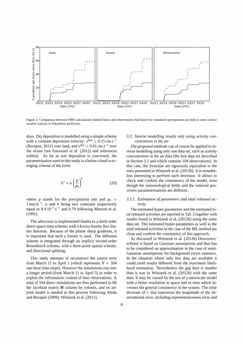
As shown in Fig. 2, WRF simulations show a goodability to model the occurrence of rain episodes but havethe general tendency to overestimate precipitation rates(Katata et al. (2012) observed the same behaviour usingMM5). This bias is a severe drawback when looking atdeposition processes as this study aims to do. To avoidoverestimating wet deposition, we used ground obser-vations of rain rates in Fukushima and Ibaraki prefec-tures to compute a global debiasing coefficient, that we

3http://www.mext.go.jp/b_menu/shingi/chousa/

gijyutu/017/shiryo/__icsFiles/afieldfile/2011/09/

02/1310688_1.pdf

found equal to 2.4, by which were divided all precipita-tion rates computed by the WRF model. We have alsotested local corrections of the precipitation fields usingdata assimilation techniques but we did not find them tobe as robust and reliable as a simpler global debiasingcorrection.

3.2.2. Atmospheric transport modelThe simulations of the dispersion of radionuclides

from the Fukushima Daiichi nuclear power plant havebeen performed with the chemistry-transport model P-3D, the Eulerian model of the P platform.It has been validated for the simulation of radionuclidestransport on the European Tracer Experiment, on the Al-geciras incident and on the Chernobyl accident (Queloet al., 2007).

The model integrates the concentration fieldc of137Cs, following the transport equation

∂c∂t+ div (uc) = div

(

ρK∇(

cρ

))

−Λs c−Λd c+σ (18)

whereρ is the air density,Λs is the scavenging rate,Λd

represents the radioactive decay andσ is the point-wisesource.K is the matrix of turbulent diffusion, diagonalin practice. The vertical component is given byKz, com-puted with Louis parametrisation (Louis, 1979). Thehorizontal componentKH is taken constant. The bound-ary condition on the ground is

Kz∇c · n = −vdepc (19)

wheren is the upward oriented unitary vector, andvdep

is the dry deposition velocity of137Cs.Two domains of simulation are considered. The finest

domain of simulation is a mesoscale domain coveringJapan, from 131.03◦E to 144.53◦E and from 30.72◦N to43.72◦N with a spatial resolution of 0.05◦ × 0.05◦. Thenumber of grid points in this domain is 270× 260. Be-cause of the small size of the domain there is a risk ofre-circulation of the plume outside the domain so thatthe model could fail to account for radionuclides re-entries. To avoid such situation and in order to com-pute the boundary conditions to this domain by a nest-ing technique, another more extended domain of sim-ulation with a coarser resolution is used. It covers aregion from 115.03◦E to 165.03◦E and from 25.02◦N to60.02◦N with a resolution of 0.25◦ × 0.25◦. This con-figuration is displayed in Fig. 1. For both domains theP3D model is configured with 15 vertical levelsranging from 0 to 8000 m.

Caesium-137 is modelled as monodispersed passiveparticulate matter with a radioactive decay of 11000

6

Table 1: Configuration and physical parametrisations of the WRFmodel. A two-way nesting technique is used between domain 1 anddomain 2.

Domain 1 2Spatial resolution 18 km 6 kmNumber of grid points 340× 250 241× 241Number of vertical levels 27 27Numerical time-step 60 s 20 sOutput time-step 3600 s 3600 sPlanetary boundary layer Yonsei University Yonsei UniversityMicro-physics Kessler WRF Single Moment 3Cumulus physics Grell-Devenyi Grell-DevenyiLongwave radiation RRTM RRTMShortwave radiation Dudhia DudhiaSurface layer MM5 similarity MM5 similarityLand surface Noah LSM Noah LSMNudging Grid nudging Grid nudging

20�N

30�N

40�N

50�N

60�N

100�E 120�E 140�E 160�E 180�

Figure 1: Map of the simulation domains used in WRF (dashed-linedomains) and in P3D (full-line domains). Two-way nesting is used inthe WRF simulations and one-way nesting in the P3D simulation. A triangle marks the location of the Fukushima Daiichi nuclear powerplant.

7

03/11 03/15 03/19 03/23 03/27 03/31Date (UTC)

0

20

40

60

80

Cum

ula

ted r

ain

(m

m)

since

20

11

-03

-11

Iitate

03/11 03/15 03/19 03/23 03/27 03/31Date (UTC)

Hirono

03/11 03/15 03/19 03/23 03/27 03/31Date (UTC)

Nihommatsu

Figure 2: Comparison between WRF calculations (dashed lines)and observations (full lines) for cumulated precipitation (in mm) at some surfaceweather stations in Fukushima prefecture.

days. Dry deposition is modelled using a simple schemewith a constant deposition velocity:vdep = 0.15 cm.s−1

(Bocquet, 2012) over land, andvdep = 0.01 cm.s−1 overthe ocean (see Estournel et al. (2012) and referenceswithin). As far as wet deposition is concerned, theparametrisation used in this study is a below-cloud scav-enging scheme of the form:

Λs = a

(

pp0

)b

(20)

where p stands for the precipitation rate andp0 =

1 mm.h−1, a and b being two constants respectivelyequal to 8.4 10−5 s−1 and 0.79 following Maryon et al.(1991).

The advection is implemented thanks to a third-orderdirect space-time scheme, with a Koren-Sweby flux lim-iter function. Because of the plume sharp gradients, itis important that such a limiter is used. The diffusionscheme is integrated through an implicit second-orderRosenbrock scheme, with a three-point spatial scheme,and directional splitting.

This study attempts to reconstruct the source termfrom March 11 to April 1 (which representsN = 504one-hour time-steps). However the simulations run overa longer period (from March 11 to April 5) in order toexploit the information content of later observations. Atotal of 504 direct simulations are thus performed to fillthe Jacobian matrixH column by column, and no ad-joint model is needed in this process following Abidaand Bocquet (2009); Winiarek et al. (2011).

3.3. Inverse modelling results only using activity con-centrations in the air

The proposed methods can of course be applied to in-verse modelling using only one data set, such as activityconcentration in the air data (the first data set describedin Section 3.1 and which contains 104 observations). Inthis case, the formulae are rigorously equivalent to theones presented in Winiarek et al. (2012b). It is nonethe-less interesting to perform such inversion. It allows tocheck and confirm the consistency of the model, eventhough the meteorological fields and the removal pro-cesses parameterisations are different.

3.3.1. Estimation of parameters and total released ac-tivity

The estimated hyper-parameters and the estimated to-tal released activities are reported in Tab. 2 together withresults found in Winiarek et al. (2012b) using the samedata set. The estimated hyper-parameters as well as thetotal released activities in the case of the ML method areclose and confirm the consistency of this approach.

As discussed in Winiarek et al. (2012b) Desroziers’scheme is based on Gaussian assumptions and thus hasto be considered an approximation in the case of semi-Gaussian assumptions for background errors statistics.In the situation where only few data are available itcould yield results different from the maximum likeli-hood estimation. Nevertheless the gap here is smallerthan it was in Winiarek et al. (2012b) with the samedata. It may be caused by the use of a mesoscale modelwith a better resolution in space and in time which in-creases the general consistency in the system. The cleardecrease ofr, that represents the magnitude of the ob-servational error, including representativeness error and

8

part of model error, was to be expected and may be dueto a better resolved model hence reducing the impact ofmodel error in the inversion.

Using the maximum likelihood estimation, the to-tal released activity of137Cs is estimated to be 1.1 ×1016 Bq. This is consistent with other estimations:1.2 × 1016Bq for Winiarek et al. (2012b) and Chinoet al. (2011), 1.3 × 1016 Bq for Terada et al. (2012),1.6 × 1016 Bq for Saunier et al. (2013), 2.1 × 1016 Bqfor Mathieu et al. (2012) or 3.6×1016 Bq for Stohl et al.(2012).

3.3.2. Temporal profile and uncertainty reduction

Due to the meteorological conditions which have of-ten transported the radionuclides towards the PacificOcean, and to the low number of activity concentrationdata, the observability of the plume is reduced. That iswhy inverse modelling methods are only able to recon-struct the source term in some specific time intervals.Consequently the estimated total released activities haveto be considered as lower bound estimates of the actualreleases.

The reconstructed source term and its uncertainty aredisplayed in Fig. 3(a). The posterior uncertainty hasbeen computed from a Monte Carlo analysis, where theobservations and the background term are perturbed us-ing their prior errors definition and the hyper-parametersestimates (2× 104 draws and inversions are performed).Then the standard deviation of the estimators ensembleis used to estimate the posterior uncertainty of the re-constructed source term. The uncertainty on the totalreleased activity is around 65%.

The time intervals of observability are clearly visiblein the shape of the uncertainty. Three periods are par-ticularly well observed: the first one lies approximatelyfrom 14 March to 15 March, the second one lies from19 March to 22 March and the last one from 24 Marchto 26 March. Once again the temporal profiles of thesource term and its uncertainty are very consistent withthe inversion made in Winiarek et al. (2012b).

Compared to source term estimates constructed fromin-situ events monitoring and core inventories (Mathieuet al., 2012), a few events are not retrieved: the firsthydrogen explosions in Unit 1 on 12 March, the vent-ings of Unit 3 on 13 March and the events concerningUnit 2 and 3 on 16 March and 18 March. On the otherhand, the multiple events of 14 March and 15 March arepresent in the reconstructed source term, even though inan incomplete way since the last release, probably be-tween 7:00 UTC and 12:00 UTC on 15 March, is miss-ing. This release is partly accounting for the north-west

pattern on the deposition map, but no activity concen-tration observation is available to help reconstruct thisevent. The releases of 20 March and the ones from 21March to 23 March are also retrieved. As far as the re-lease around 25 March is concerned, there seems to bea slight offset of 12 hours in the reconstruction. The re-leases reconstructed on 19 March are not mentioned bythese inventories, but seem compatible with the in-situmeasurements ofγ-dose rates from operator TEPCO4,for example on the northside of main office or near thewest gate of the NPP. They are also retrieved by Stohlet al. (2012). They precede the attempts of emergencycooling with Tokyo Fire Department means. Finally, thereleases around 30 March, not mentioned by the formerinventories, are also retrieved by Terada et al. (2012).

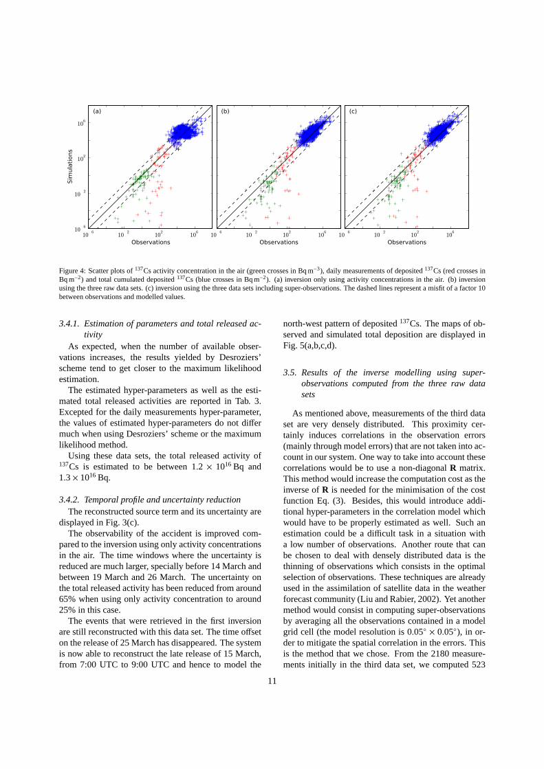
The scatter plot of all observations is displayed inFig. 4(a). The simulation using the source term re-constructed with activity concentration data only doesnot show any systematic bias when estimating the de-posited activities. Again, this shows the consistencyof the model and in particular of the removal processes(wet and dry deposition).

3.4. Results of the inverse modelling using the three rawdata sets

The total deposited137Cs measurements offer no in-formation about the time of deposition as they are mea-surements performed a posteriori, in May and June2011. When only these measurements are used toattempt reconstructing the source term, the total re-leased estimated activity seems consistent (between1.1 × 1016 Bq and 1.2 × 1016 Bq). However, the tem-poral profile, displayed in Fig. 3(b), is highly doubtful.Only releases on 23 and on 25 March are clearly visi-ble. Indeed, the system has too much freedom to fit thedata. The only constraint is the background term in thecost function, which in the case where the first guessis taken null (as we do) only defines a scale of ampli-tude. Therefore, even if these observations are abun-dant with a good spatial distribution, we propose in thenext sections to jointly use them with other measure-ments with a good temporal resolution, such as activityconcentrations in the air and daily measurements of de-posited material. Consequently we propose to use thethree data sets described in Section 3.1 in the same in-version. In this aim the prior errors have to be estimatedsimultaneously for the background and the three datasets (Nd = 3).

4http://www.tepco.co.jp/en/nu/monitoring/index-e.

html

9

Table 2: Estimation of parameters and corresponding reconstructed released activity for caesium-137 source reconstruction using only activityconcentration observations in the air.

parameter method Regional scale model Mesoscale modelWiniarek et al. (2012b) This study

r (Bq m−3)Desroziers’ scheme 5.4 2.1Maximum likelihood 3.3 1.9

m(Bq s−1)Desroziers’ scheme 5.3× 1010 8.9× 1010

Maximum likelihood 2.0× 1011 1.6× 1011

Released activity (Bq)Desroziers’ scheme 3.3× 1015 7.2× 1015

Maximum likelihood 1.2× 1016 1.1× 1016

03/11 03/13 03/15 03/17 03/19 03/21 03/23 03/25 03/27 03/29 03/31

Date (UTC)

109

1010

1011

1012

Sourc

e R

ate

(B

q/s

)

(a)

03/11 03/13 03/15 03/17 03/19 03/21 03/23 03/25 03/27 03/29 03/31

Date (UTC)

109

1010

1011

1012

Sourc

e R

ate

(B

q/s

)(b)

03/11 03/13 03/15 03/17 03/19 03/21 03/23 03/25 03/27 03/29 03/31

Date (UTC)

109

1010

1011

1012

Sourc

e R

ate

(B

q/s

)

(c)

03/11 03/13 03/15 03/17 03/19 03/21 03/23 03/25 03/27 03/29 03/31

Date (UTC)

109

1010

1011

1012

Sourc

e R

ate

(B

q/s

)

(d)

Figure 3: Full line: Temporal profile of reconstructed caesium-137 source term using (a): activity concentration of137Cs measurements in the aironly, (b): total cumulated deposited137Cs measurements only, (c): the activity concentration in the air, the daily fallout measurements and thetotal cumulated deposition raw measurements, (d): the activity concentration in the air, the daily fallout measurements andthe super-observationscomputed from the total cumulated deposited137Cs. Dashed lines: posterior uncertainty of the source term computed using a Monte Carlosimulation.

10

10✁6

10✁2

102

106

Observations

10✁610✁2102

106

Sim

ulations

(a)

10✁6

10✁2

102

106

Observations

(b)

10✁6

10✁2

102

106

Observations

(c)

Figure 4: Scatter plots of137Cs activity concentration in the air (green crosses in Bq m−3), daily measurements of deposited137Cs (red crosses inBq m−2) and total cumulated deposited137Cs (blue crosses in Bq m−2). (a) inversion only using activity concentrations in the air. (b) inversionusing the three raw data sets. (c) inversion using the three data sets including super-observations. The dashed lines represent a misfit of a factor 10between observations and modelled values.

3.4.1. Estimation of parameters and total released ac-tivity

As expected, when the number of available obser-vations increases, the results yielded by Desroziers’scheme tend to get closer to the maximum likelihoodestimation.

The estimated hyper-parameters as well as the esti-mated total released activities are reported in Tab. 3.Excepted for the daily measurements hyper-parameter,the values of estimated hyper-parameters do not differmuch when using Desroziers’ scheme or the maximumlikelihood method.

Using these data sets, the total released activity of137Cs is estimated to be between 1.2 × 1016 Bq and1.3× 1016 Bq.

3.4.2. Temporal profile and uncertainty reductionThe reconstructed source term and its uncertainty are

displayed in Fig. 3(c).The observability of the accident is improved com-

pared to the inversion using only activity concentrationsin the air. The time windows where the uncertainty isreduced are much larger, specially before 14 March andbetween 19 March and 26 March. The uncertainty onthe total released activity has been reduced from around65% when using only activity concentration to around25% in this case.

The events that were retrieved in the first inversionare still reconstructed with this data set. The time offseton the release of 25 March has disappeared. The systemis now able to reconstruct the late release of 15 March,from 7:00 UTC to 9:00 UTC and hence to model the

north-west pattern of deposited137Cs. The maps of ob-served and simulated total deposition are displayed inFig. 5(a,b,c,d).

3.5. Results of the inverse modelling using super-observations computed from the three raw datasets

As mentioned above, measurements of the third dataset are very densely distributed. This proximity cer-tainly induces correlations in the observation errors(mainly through model errors) that are not taken into ac-count in our system. One way to take into account thesecorrelations would be to use a non-diagonalR matrix.This method would increase the computation cost as theinverse ofR is needed for the minimisation of the costfunction Eq. (3). Besides, this would introduce addi-tional hyper-parameters in the correlation model whichwould have to be properly estimated as well. Such anestimation could be a difficult task in a situation witha low number of observations. Another route that canbe chosen to deal with densely distributed data is thethinning of observations which consists in the optimalselection of observations. These techniques are alreadyused in the assimilation of satellite data in the weatherforecast community (Liu and Rabier, 2002). Yet anothermethod would consist in computing super-observationsby averaging all the observations contained in a modelgrid cell (the model resolution is 0.05◦ × 0.05◦), in or-der to mitigate the spatial correlation in the errors. Thisis the method that we chose. From the 2180 measure-ments initially in the third data set, we computed 523

11

(a)

37.5✂N

(b)

(c)

37.5✂N

140✂E

(d)

140✂E

10 30 60 100 300 600 1000 3000

Figure 5: Map of observed and simulated deposited137Cs. Upper left (a): measurements from MEXT. Upper right (b): simulation with sourcereconstructed using only137Cs activity concentrations in the air. Lower left (c): simulation with source reconstructed using137Cs activity concen-trations in the air, daily measurements of deposited137Cs and measurements of total cumulated deposited137Cs. Lower right (d): simulation withsource reconstructed using137Cs activity concentrations in the air, daily measurements of deposited137Cs and super-observations computed frommeasurements of total cumulated deposited137Cs. The displayed values are in kBq m−2

12

Table 3: Estimation of parameters and corresponding reconstructed released activity for caesium-137 source using activity concentration, falloutdaily measurements and total deposition data.r1, r2 andr3 represents respectively the errors variances of these three data sets.

parameter method with deposition with depositionraw data super-observations

r1 (Bq m−3)Desroziers’ scheme 3.8 2.9Maximum likelihood 3.3 2.3

r2 (Bq m−2)Desroziers’ scheme 580 540Maximum likelihood 210 240

r3 (Bq m−2)Desroziers’ scheme 325000 240000Maximum likelihood 320000 230000

m(Bq s−1)Desroziers’ scheme 1.2× 1011 1.3× 1011

Maximum likelihood 1.0× 1011 1.0× 1011

Released activity (Bq)Desroziers’ scheme 1.3× 1016 1.9× 1016

Maximum likelihood 1.2× 1016 1.8× 1016

super-observations from which we eliminated 4 super-observations located too close to the NPP, hence leaving519 super-observations to be used as the new third dataset. Note that it is not necessary to estimate the reducedvariance of a super-observation since this is implicitlyaccounted for in the related hyper-parameter estimation.

3.5.1. Estimation of parameters and total released ac-tivity

The estimated hyper-parameters as well as the esti-mated total released activities are reported in Tab. 3. Asexpected, the estimated standard deviation of the errorin the cumulated fallout (r3) is significantly decreasedby about 28%.

Using these data sets, the total released activity of137Cs is estimated to be between 1.8 × 1016 Bq and1.9× 1016 Bq.

3.5.2. Temporal profile and uncertainty reductionThe reconstructed source term and its uncertainty are

displayed in Fig. 3(d). The uncertainty on the total re-leased activity is estimated to be around 15% from aMonte Carlo study of 2× 104 draws. However, it is thesame absolute standard deviation, of about 3 PBq, as inthe raw data sets inversion.

All the previously mentioned events are now retrievedwith these data sets:

• Around 12 March: identified as the hydrogen ex-plosion in Unit 1.

• On 13 March: identified as the ventings on Unit 3.

• On 14 and 15 March: multiple ventings and hy-drogen explosions mainly concerning Unit 2 and

Unit 3. The late release on 15 March is now re-trieved (from 7:00 to 9:00 UTC) even if its magni-tude might appear weak (see section 3.6.1 for a dis-cussion on the magnitude of the retrieved peaks).

• On 16 March: unidentified events but which corre-spond to pressure drops in Unit 2 and Unit 3.

• On 18 March: unidentified events probably relatedto Unit 3.

• On 19 March: unidentified events which corre-spond to an increase in several in-situγ-dose ratemeasurements. The attempts of emergency coolingwith the Tokyo Fire Department means began justafter these events.

• On 20 March: unidentified events concerning atleast Unit 2 and Unit 3.

• From 21 March to 23 March: events correspondingto smokes emitted from Unit 2 and Unit 3.

• On 25 March: unidentified event possibly concern-ing Unit 2. The magnitude of this peak might ap-pear over-estimated (see section 3.6.1 for a discus-sion on the magnitude of the retrieved peaks).

• On 30 March: unidentified event.

From the scatter plots of Fig. 4(b,c), it is clear thatthe simulated cumulated deposition data are comparablewhen using the source term built from raw data or fromsuper-observations. This is also visible on the deposi-tion maps in Fig. 5(c,d). On the other hand the system’sability to simulate the two other data sets is slightly im-proved when using the source term retrieved from thesuper-observations. The assumption that the observa-tion errors are uncorrelated led the system to give too

13

much weight to the third raw data set in the inversemodelling algorithm. This over-confidence may be cor-rected when using super-observations so that the infor-mation content in the system is better balanced.

3.6. Discussion about the retrieved sourcesThese inversions offer an objective estimation using

data assimilation techniques of what can be extractedfrom the data sets and the numerical model. The assim-ilated observations may or may not suffice to constrainthe source term parameters. We showed that the cumu-lated deposition data alone are not sufficient to offer asatisfying chronology of the source term and that thejoint assimilation of the three data sets helped to bet-ter constrain the chronology. Yet, the magnitude of theidentified peaks remains questionable. The data may ormay not be able to constrain them well enough, althoughthe estimate of the total released activity seems robust.

3.6.1. On the magnitude of the peaksIt is generally thought that the main releases have oc-

curred around March 15. These releases probably con-tributed the most to the north-west pattern of the deposi-tion map. Our system, where the cumulated depositiondata do not contain any information in time, may not beconstrained enough by air concentration observations ordaily measurements of fallout (specially before March18) to precisely balance the contributions of the releasesof March 14-15 (around 15% of the total retrieved ac-tivity), March 20 (around 13%) and March 25 (around15%).

The peaks of March 20 and March 25 are not only re-constructed with the help of deposition measurements.They are both additionally explained by measurementsof activity in the air from a particular monitoring sta-tion, located in Fukushima city, which measured an ac-tivity concentration of about 32 Bq.m−3 around March20 and about 14 Bq.m−3 around March 25. It is possiblethat these measurements are caused by a re-suspensionof previously deposited caesium-137. But resuspensionis not implemented in our model, so that resuspensionevents are likely to be accounted for by fictitious re-leases in the source term. We tried and performed a newinversion using the same data as in Section 3.5 but with-out the measurements of this station. Indeed, the resultsfrom the super-observations showed an increase of thereleased activity on March 14 and 15, from 2.6 to 3.0PBq (from 13% to 16% of an unchanged total emittedactivity of 19 PBq), and a decrease on March 20, from2.6 to 2.0 PBq (from 13% to 11% of the total emittedactivity). Yet, no consequences were observed on themagnitude of the peak on March 25.

We also performed inversions using a non-null firstguess inferred from independentγ-dose measurements(Saunier et al., 2013), which indicates to the system thatmost of the releases occurred before March 18. As aresult, the total estimated released activity increased byabout 15%, but the peak on March 25 still remained al-most at the same level.

As a more drastic test and to force the system toreconstruct higher releases before March 18, we re-duced the inversion window to this period. As a con-sequence the releases of March 15 increased (from0.6 PBq to 2.6 PBq using the three raw data sets, andfrom 0.9 PBq to 3.9 PBq using the three data sets withsuper-observations as the third data set), but the total es-timated releases decreased (respectively from 12 PBq to5 PBq, and from 18 PBq to 11 PBq). It is consistent withthe inversion using only activity concentration in the airwhere approximatively 6 PBq were estimated to be re-leased after this date. At the same time the reanalysisof deposition map has been degraded especially in thecentral area of the north-west pattern which is the mostcontaminated. This shows that: (i) considering only thisshorter time window, the system can not properly recon-struct the deposition pattern shown in Fig. 5(a). (ii) Re-leases probably occurred after March 19 and may havecontributed to the north-west pattern of the depositionmap, but their magnitude is still difficult to estimate be-cause of the lack of observations with a temporal infor-mation (such as activity concentration in the air) in thisarea. (iii) This may highlight the difficulty to model theremoval processes and specially the wet deposition. It isalso possible that the cumulated deposition map, whosemeasurements have been made several months after theaccident, is not anymore faithful to the deposition eventsof the accident.

We also tested a different reconstruction resolution.Instead of reconstructing a source term with a one-hourtime-step (N = 504), an inversion was carried out ona source term with a three-hour time-step (N = 168).It is generally admitted that the inversion is sensitive tothe resolution of the control space (Bocquet et al., 2011)and that the system cannot generally provide reliable in-formation at a too precise resolution (for instance themodel resolution). Nevertheless, estimating the priorerrors allows to compensate the impact of the controlspace resolution by tuning regularisation in the inver-sion, so that the dependence in the resolution should bemitigated. The estimated source term, using the samedata sets as in Section 3.5, as well as its uncertaintyare displayed in Fig. 6. The total released activity isnow estimated to be 1.6 × 1016 Bq with an uncertaintyof 18%. The estimated released quantities were mainly

14

11/03 13/03 15/03 17/03 19/03 21/03 23/03 25/03 27/03 29/03 31/03Date (UTC)

10

10

10

10

Sou

rce

rate

(B

q/s)

9

10

11

12

Figure 6: Full black line: Temporal profile of reconstructed caesium-137 source term with a reconstruction resolution of 3 h usingtheactivity concentration in the air, the daily fallout measurements andthe super-observations computed from the total cumulated deposited137Cs. Dashed line: posterior uncertainty of the source term computedusing a Monte Carlo simulation. Thin blue line: Temporal profile ofreconstructed caesium-137 source term with a reconstruction resolu-tion of 1 h using the same data.

reduced on March 30 (from 2.1 PBq to 1.3 PBq), onMarch 20 (from 2.6 PBq to 2.1 PBq) and on March 25(from 2.9 PBq to 2.8 PBq), but remain at a high level.At the same time, the estimated released quantities in-creased on March 14-15 from 2.6 PBq to 4.1 PBq. Manyof the low magnitude peaks with a high uncertainty havebeen reduced or have disappeared.

3.6.2. On the difference between the sources recon-structed with raw data and super-observations

Comparing the source profile obtained from thesuper-observations (Fig. 3(d)) with the source pro-file obtained from the inversion of the raw data sets(Fig. 3(c)), 2 PBq of caesium-137 are found to increasealready existing peaks.

Moreover, when using super-observations instead ofraw data, new release episodes appear in the source re-constructed term. Compared to the raw data sets in-version, 4 PBq of caesium-137 are found in new timeslots.Yet the related uncertainty is still high and evenabove the retrieved peaks. Nonetheless, the new re-leases episodes that appear in the inversion do not seemto be artefacts of the inversion algorithm. They do cor-respond to observed events in the NPP and to events re-constructed by other studies (Stohl et al., 2012; Saunieret al., 2013).

Judging from the r i , the errors of the super-observations as well as their use by the model is di-

agnosed as more reliable than the use of the raw datasets. By contrast, the Tikhonov regularising term is lessconstraining and new peaks can more easily form in thereconstructed source term.

On a physical level, the appearance of the new peaksresults from the smoothing of the deposition observa-tions that in turn leads to a smoothing in the retrievedsource. This is probably why the only peak which is re-duced when using super-observations is the highest oneon March 25. This peak is mainly induced by the137Csdeposit observations of the north-west very thin pattern.Hence, a smoothing of this pattern can lead to a new bal-ance of the peaks (March 15, March 20 or March 25).

4. Conclusion

In order to reconstruct source terms of accidental pol-lutant releases into the atmosphere, we have proposedan inverse modelling algorithm able to use all avail-able data in the same inversion (concentrations in theair, measurements of fallout, integrated measurements,etc.). The algorithm relies on the relationship providedby the atmospheric transport model between the sourcevector and the observation set and on prior errors in-troduced in the system: the background errors and theobservation errors. To properly balance the informationcontent in the system a proper estimation of these priorerrors is crucial.

In this aim, we proposed two methods relying onthe maximum likelihood principle that we applied tothe challenging reconstruction of the137Cs source termreleased during the Fukushima Daiichi nuclear powerplant accident in March 2011. Three data sets wereused in the inversion process: activity concentrations inthe air, daily measurements of fallout and total cumu-lated deposition data. Consequently, the prior estima-tion concerned 4 hyper-parameters: the variance of thebackground errors and the variance of each observationset errors. Averaged observations (called in the articlesuper-observations) have also been considered for thethird data set in order to reduce correlation in errors thathad been neglected in the algorithm. Posterior uncer-tainty related to the estimated releases have also beenestimated through a Monte Carlo analysis. Such an es-timation is only possible with properly estimated priorerrors.

With these methods and without super-observations,the total released activity is estimated to be between1.2 − 1.3 × 1016 Bq with a related uncertainty around25%. When using super-observations instead of rawfallout data, the total released activity is estimated to bebetween 1.8 − 1.9 × 1016 Bq with a related uncertainty

15

around 15%. From our estimations the main137Cs con-tamination over Japan results from releases on 14-15March, 19-20 March, 25 March and 30 March. Nev-ertheless, the uncertainty of each retrieved peak still re-mains high. Consequently the exact magnitude of theretrieved peaks has to be handled carefully. Some othersignificant releases might also have occurred when thewind was blowing directly towards the Pacific Oceanand are thus not totally reconstructed by our method us-ing only data over Japan.

With the given data sets, the reconstruction of thesource term could be improved on the condition thatmodel error be better constrained. Two main influen-tial sources of error were identified in the course of thisstudy. Firstly, the reconstruction was found to be highlysensitive to the precipitation fields of the meteorologicalmodel. Even if the spatial distribution and chronologyof the precipitation events were matching independentprecipitation observations, we found it difficult to prop-erly estimate the magnitude of those events. Secondly,with the given precipitation fields, the reconstruction re-mains sensitive to the physical process parameterisationin the ATM. One promising route to better constrainthose processes is the inverse modelling of physical pa-rameters (Bocquet, 2012).

Finally it seems promising to develop methods ableto simultaneously reconstruct source terms of severalradionuclides using all available data includingγ-doserates (Saunier et al., 2013). The number of observa-tions, and in particular observations with an informationof time, would then increase substantially. But the in-volved methods would certainly be more complex own-ing to correlations in observation errors and higher prioruncertainties in the data assimilation system.

5. Acknowledgements

This study has been supported by the IMMANENTproject of Paris-Est University, and by the INSU/LEFE-ASSIM project ADOMOCA-2.

References

Abida, R., Bocquet, M., 2009. Targeting of observations foraccidentalatmospheric release monitoring. Atmos. Env. 43, 6312–6327.

Anderson, J. L., 2007. An adaptive covariance inflation error correc-tion algorithm for ensemble filters. Tellus A 59, 210–224.

Bocquet, M., 2005. Reconstruction of an atmospheric tracer sourceusing the principle of maximum entropy. I: Theory. Q. J. R. Mete-orolog. Soc. 131, 2191–2208.

Bocquet, M., 2012. Parameter field estimation for atmospheric disper-sion: Application to the Chernobyl accident using 4D-Var. Q. J. R.Meteorolog. Soc. 138, 664–681.

Bocquet, M., Pires, C. A., Wu, L., 2010. Beyond Gaussian statisticalmodeling in geophysical data assimilation. Mon. Wea. Rev. 138,2997–3023.

Bocquet, M., Wu, L., Chevallier, F., 2011. Bayesian design of con-trol space for optimal assimilation of observations. I: Consistentmultiscale formalism. Q. J. R. Meteorolog. Soc. 137, 1340–1356.

Byrd, R. H., Lu, P., Nocedal, J., 1995. A limited memory algorithmfor bound constrained optimization. SIAM Journal on Scientificand Statistical Computing 16, 1190–1208.

Chapnik, B., Desroziers, G., Rabier, F., Talagrand, O., 2004. Proper-ties and first application of an error-statistics tuning method in vari-ational assimilation. Q. J. R. Meteorolog. Soc. 130, 2253–2275.

Chapnik, B., Desroziers, G., Rabier, F., Talagrand, O., 2006. Diag-nosis and tuning of observational error in a quasi-operational dataassimilation setting. Q. J. R. Meteorolog. Soc. 132, 543–565.

Chino, M., Nakayama, H., Nagai, H., Terada, H., Katata, G., Ya-mazawa, H., 2011. Preliminary estimation of release amounts ofI131 and Cs137 accidentally discharged from the Fukushima Dai-ichi nuclear power plant into the atmosphere. Journal of NuclearScience and Technology 48, 1129–1134.

Davoine, X., Bocquet, M., 2007. Inverse modelling-based reconstruc-tion of the Chernobyl source term available for long-range trans-port. Atmos. Chem. Phys. 7, 1549–1564.

Dee, D. P., 1995. On-line estimation of error covariance parametersfor atmospheric data assimilation. Mon. Wea. Rev. 123, 1128–1145.

Delle Monache, L., Lundquist, J. K., Kosovic, B., Johannesson, G.,Dyer, K. M., Aines, R. D., Chow, F. K., Belles, R. D., Hanley,W. G., Larsen, S. C., Loosmore, G. A., Nitao, J. J., Sugiyama,G. A., Vogt, P. J., 2008. Bayesian inference and Markov chainMonte Carlo sampling to reconstruct a contaminant source on acontinental scale. Journal of Applied Meteorology and Climatol-ogy 47, 2600–2613.

Desroziers, G., Berre, L., Chapnik, B., Poli, P., 2005. Diagnosis ofobservation, background and analysis error statistics in observationspace. Q. J. R. Meteorolog. Soc. 131, 3385–3396.

Desroziers, G., Ivanov, S., 2001. Diagnosis and adaptive tuning ofobservation-error parameters in a variational assimilation. Q. J. R.Meteorolog. Soc. 127, 1433–1452.

Elbern, H., Strunk, A., Schmidt, H., Talagrand, O., 2007. Emissionrate and chemical state estimation by 4-dimensional variational in-version. Atmos. Chem. Phys. 7, 3749–3769.

Estournel, C., Bosc, E., Bocquet, M., Ulses, C., Marsaleix,P.,Winiarek, V., Osvath, I., Nguyen, C., Duhaut, T., Lyard, F.,Michaud, H., Auclair, F., 2012. Assessment of the amount ofcesium-137 released to the Pacific Ocean after the Fukushima ac-cident and analysis of its dispersion in the Japanese coastal waters.J. Geophys. Res. 117, C11014.

Hajivassiliou, V., McFadden, D., Ruud, P., 1996. Simulationof multi-variate normal rectangle probabilities and their derivatives - Theo-retical and computational results. Journal of Econometrics 72, 85–134.

Hansen, P. C., 1992. Analysis of discrete ill-posed problemsby meansof the L-curve. SIAM Review 34, 561–580.

Katata, G., Terada, H., Nagai, H., Chino, M., 2012. Numericalrecon-struction of high dose rate zones due to the Fukushima Dai-ichiNuclear Power Plant accident. J. Environ. Radioactivity 111, 2–12.

Korsakissok, I., Mathieu, A., Didier, D., 2013. Atmosphericdisper-sion and ground deposition induced by the Fukushima NuclearPower Plant accident: A local-scale simulation and sensitivitystudy. Atmos. Env. 70, 267–279.

Krysta, M., Bocquet, M., Brandt, J., 2008. Probing ETEX-II data setwith inverse modelling. Atmos. Chem. Phys. 8, 3963–3971.

Li, H., Kalnay, E., Miyoshi, T., 2009. Simultaneous estimation ofcovariance inflation and observation errors within an ensemble

16

Kalman filter. Q. J. R. Meteorolog. Soc. 135, 523–533.Liu, Z.-Q., Rabier, F., 2002. The interaction between model resolu-

tion, observation resolution and observation density in data assim-ilation: A one-dimensional study. Q. J. R. Meteorolog. Soc. 128,1367–1386.

Louis, J., 1979. A parametric model of vertical eddy fluxes in theatmosphere. Boundary-Layer Meteor. 17, 197–202.

Maryon, R. H., Smith, F. B., Conway, B. J., Goddard, D. M., 1991.The U.K. nuclear accident model. Progress in Nuclear Energy 26,85–104.

Mathieu, A., Korsakissok, I., Quelo, D., Groell, J., Tombette, M., Di-dier, D., Quentric, E., Saunier, O., Benoit, J.-P., Isnard,O., 2012.Atmospheric dispersion and deposition of radionuclides from theFukushima Daiichi nuclear power plant accident. Elements 8, 195–200.

Menard, R., Cohn, S. E., Chang, L.-P., Lyster, P. M., 2000. Assimila-tion of stratospheric chemical tracer observations using a Kalmanfilter. Part I: Formulation. Mon. Wea. Rev. 128, 2654–2671.

Michalak, A. M., Bruhwiler, L., Tans, P. P., 2004. A geostatisticalapproach to surface flux estimation of atmospheric trace gases. J.Geophys. Res. 109, D14109.

Mitchell, H. L., Houtekamer, P. L., 1999. An adaptive ensembleKalman filter. Mon. Wea. Rev. 128, 416–433.

Quelo, D., Krysta, M., Bocquet, M., Isnard, O., Minier, Y., Sportisse,B., 2007. Validation of the Polyphemus platform on the ETEX,Chernobyl and Algeciras cases. Atmos. Env. 41, 5300–5315.

Saide, P., Bocquet, M., Osses, A., Gallardo, L., 2011. Constrainingsurface emissions of air pollutants using inverse modeling: methodintercomparison and a new two-step multiscale approach. Tellus B63, 360–370.

Saunier, O., Mathieu, A., Didier, D., Tombette, M., Quelo, D.,Winiarek, V., Bocquet, M., 2013. An inverse modeling method toassess the source term of the Fukushima nuclear power plant ac-cident using gamma dose rate observations. Atmos. Chem. Phys.Discuss. 13, 15567–15614.

Schwinger, J., Elbern, H., 2010. Chemical state estimation for themiddle atmosphere by four dimensional variational data assimila-tion: A posteriori validation of error statistics in observation space.J. Geophys. Res. 115, D18307.

Skamarock, W. C., Klemp, J. B., Dudhia, J., Gill, D. O., Barker,D. M.,Duda, M. G., Huang, S.-Y., Wang, W., Powers, J. G., 2008. Adescription of the advanced research WRF version 3. Tech. rep.,NCAR.

Stauffer, D. R., Seaman, N. L., 1994. On multi-scale four dimensionaldata assimilation. J. Appl. Meteor. 33, 416–434.

Stohl, A., Seibert, P., Wotawa, G., Arnold, D., Burkhart, J.F.,Eckhardt, S., Vargas, A., Yasunari, T. J., 2012. Xenon-133 andcaesium-137 releases into the atmosphere from the FukushimaDai-ichi nuclear power plant: determination of the source term,atmospheric dispersion, and deposition. Atmos. Chem. Phys. 12,2313–2343.

Terada, H., Katata, G., Chino, M., Nagai, H., 2012. Atmospheric dis-charge and dispersion of radionuclides during the FukushimaDai-ichi Nuclear Power Plant accident. Part ii: verification of the sourceterm and analysis of regional-scale atmospheric dispersion. J. En-viron. Radioactivity 112, 141–154.

Winiarek, V., Bocquet, M., Saunier, O., Mathieu, A., 2012a.Cor-rection to ”Estimation of errors in the inverse modeling of acci-dental release of atmospheric pollutant: Application to therecon-struction of the cesium-137 and iodine-131 source terms from theFukushima Daiichi power plant”. J. Geophys. Res. 117, D18118.

Winiarek, V., Bocquet, M., Saunier, O., Mathieu, A., 2012b.Esti-mation of errors in the inverse modeling of accidental releaseofatmospheric pollutant: Application to the reconstruction of thecesium-137 and iodine-131 source terms from the Fukushima Dai-

ichi power plant. J. Geophys. Res. 117, D05122.Winiarek, V., Vira, J., Bocquet, M., Sofiev, M., Saunier, O.,2011.

Towards the operational estimation of a radiological plume us-ing data assimilation after a radiological accidental atmosphericrelease. Atmos. Env. 45, 2944–2955.

Yee, E., Lien, F.-S., Keats, A., D’Amours, R., 2008. Bayesianin-version of concentration data: Source reconstruction in the adjointrepresentation of atmospheric diffusion. Journal of Wind Engineer-ing and Industrial Aerodynamics 96, 1805–1816.

17