Estimation of the Consumer Demand System in Postwar Japan

Sasaki, K.

IIASA Collaborative PaperApril 1982

Sasaki, K. (1982) Estimation of the Consumer Demand System in Postwar Japan. IIASA Collaborative Paper.

IIASA, Laxenburg, Austria, CP-82-014 Copyright © April 1982 by the author(s). http://pure.iiasa.ac.at/2104/ All

rights reserved. Permission to make digital or hard copies of all or part of this work for personal or classroom

use is granted without fee provided that copies are not made or distributed for profit or commercial advantage.

All copies must bear this notice and the full citation on the first page. For other purposes, to republish, to post on

servers or to redistribute to lists, permission must be sought by contacting repository@iiasa.ac.at

NOT FOR QUOTATiON WITHOUT PERMISSION O F THE AUTHOR

ESTIMATION OF THE CONSUMER DEMAND SYSTEM IN POSTWAR JAPAN

Kozo Sasaki

April 1982 CP-82-14

INTERNATIONAL INSTITUTE FOR APPLIED SYSTEMS ANALYSIS A-2361 L a x e n b u r g , A u s t r i a

PREFACE

Ths paper is intended to present an analytical model of a consumer demand system and to give an example of its application to empirical data in postwar Japan. The model is called Powell's system, a type of linear expenditure system.

The linear expenditure system has been used by IIASA as a method of carry- ing out the analysis and prediction of the demand side in various national models concerned with the Food and Agriculture Program (FAP). It is hoped that t h s paper will be of some help in assessing the emciency and usefulness of the linear expenditure system in the process of advancing the task at IIASA.

ACKNOWLEDGEMENTS

The author is very grateful to Mr. E. Arakawa, Secretary General of the Japan Committee for IIASA, and the parties concerned, who nominated him as a participant to the Status Report Conference of the Food and Agriculture Pro- gram in Laxenburg, February 16-18, 1981. I t provided the author with the opportunity to present the original version of t h s paper in the Conference. He is also grateful to Professor K.S. Parikh, Dr. K. Frohberg and Professor Y. Maru- yama, who made possible the distribution of t h s paper as an IIASA Collaborative Paper. Mr. Y. Fukagawa was very helpful in conducting the computation required for t h s study. Ms. Marianne Spak, Bonnie Riley and Stefanie Hoffmann were also very helpful and efficient in preparing the paper.

FOREWORD

Understanding the nature and dimensions of the world food problem and the policies available t o alleviate it has been the focal point of the IIASA Food and Agriculture Program since it began in 1977.

National food systems are highly interdependent, and yet the major policy options exist at the national level. Therefore, to explore these options, it is necessary both to d.evelop policy models for national economies and to link them together by trade and capital transfers. For greater realism the models in this scheme are being kept descriptive, rather than normative. In the end i t is proposed to' link models to twenty countries, whch together account for nearly 80 per cent of important agricultural attributes such as area, production, popu- lation, exports, imports and so on.

The linear expenditure system used by the Food and Agriculture Program for analysls and description of the demand side within the national models is examined in both a static and a dynamic version by Kozo Sasaki for the case of postwar Japan. This is a further step towards the development of a detailed agricultural model for Japan.

Gr i t Parikh Program Leader

CONTENTS

INTRODUCTION METHOD

2.1. Static Model of the Linear Expenditure System 2.2. Dynamic model: introduction of the taste variable

ESTIMATION PROCEDURE DATA AND ESTIMATION EMPIRICAL RESULTS OF THE STATIC MODEL

5.1. Estimates of Demand Parameters 5.2. Demand Elasticities 5.3. Money Flexibilities

EMPIRICAL RESULTS OF THE DYNAMIC MODEL 6.1. Estimates of Demand Parameters 6.2. Demand Elasticities 6.3 . Cost of Living Index and Subsistence Cost

CONCLUDING REMNIKS NOTES REFERENCES

This paper was o r i g i n a l l y prepared under t h e t i t l e "Modell ing f o r Management" f o r p r e s e n t a t i o n a t a Nater Research Centre (U.K. ) Conference on "River P o l l u t i o n Cont ro l " , Oxford, 9 - 1 1 A s r i l , 1979.

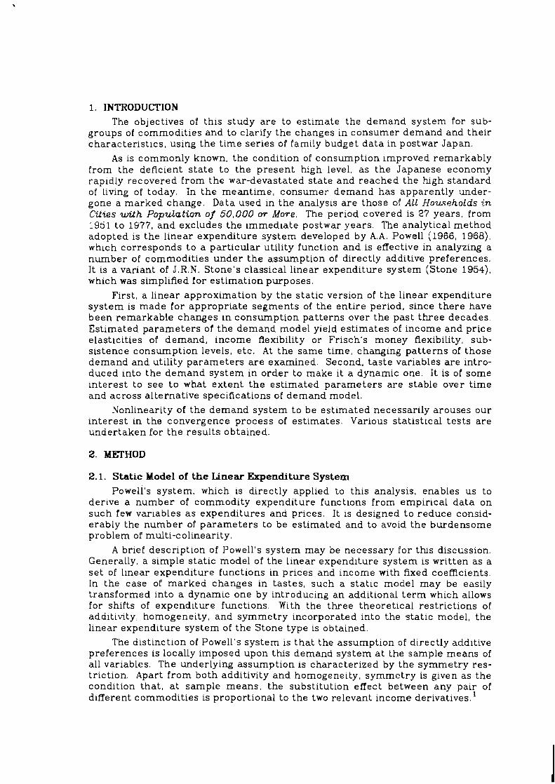
1. INTRODUCTION The objectives of this study are to estimate the demand system for sub-

groups of commodities and to clarify the changes in consumer demand and their characteristics, using the time series of family budget data in postwar Japan.

As is commonly known, the condition of consumption improved remarkably from the deficient state to the present h g h level, as the Japanese economy rapidly recovered from the war-devastated state and reached the h g h standard of living of today. In the meantime, consumer demand has apparently under- gone a marked change. Data used in the analysis are those of All H o u s e h o l d s in C i t i e s with P o p u l a t i o n o f 50,000 o r More. The period covered is 27 years, from 1951 to 1977, and excludes the immediate postwar years. The analytical method adopted is the linear expenditure system developed by A.A. Powell (1966, 1968), which corresponds to a particular utility function and is effective in analyzing a number of commodities under the assumption of directly additive preferences. It is a variant of J.R.N. Stone's classical linear expenditure system (Stone 1954), which was simplified for estimation purposes.

First, a linear approximation by the static version of the linear expenditure system is made for appropriate segments of the entire period, since there have been remarkable changes in consumption patterns over the past t h e e decades. Estimated parameters of the demand model yield estimates of income and price elasticities of demand, income flexibility or Frisch's money flexibility, sub- sistence consumption levels, etc. At the same time, changing patterns of those demand and utility parameters are examined. Second, taste variables are intro- duced into the demand system in order to make it a dynamic one. It is of some interest to see to what extent the estimated parameters are stable over time and across alternative specifications of demand model.

Nonlinearity of the demand system to be estimated necessarily arouses our interest in the convergence process of estimates. Various statistical tests are undertaken for the results obtained.

2. METHOD

2.1. Static Model of tAe Linear Expenditure System Powell's system, which is directly applied to this analysis, enables us to

derive a number of commodity expenditure functions from empirical data on such few variables as expenditures and prices. It is designed to reduce consid- erably the number of parameters to be estimated and to avoid the burdensome problem of multi-colinearity.

A brief description of Powell's system may be necessary for thls discussion. Generally, a simple static model of the linear expenditure system is written as a set of linear expenditure functions in prices and income with fixed coefficients. In the case of marked changes in tastes, such a static model may be easily transformed into a dynamic one by introducing an additional term which allows for shifts of expenditure functions. With the three theoretical restrictions of additivity, homogeneity, and symmetry incorporated into the static model, the linear expenditure system of the Stone type is obtained.

The distinction of Powell's system is that the assumption of directly additive preferences is locally imposed upon t h s demand system a t the sample means of all variables. The underlying assumption is characterized by the symmetr-y res- triction. Apart from both adhtivity and homogeneity, symmetry is given as the condition that, a t sample means, the substitution effect between any pair of different commodities is proportional to the two relevant income derivatives. '

Thus the static model is transformed into the following expression:

where

zit = biCjbj(pjt/Fj - ~it/Fi)B (1, j = I , 2 , . . . , N) (2)

~t = mt - CjpjtYj (3)

The vit, pit, and xit indicate per capita expenditure on the i* commodity, the price of the^& commodity, and the quantity consumed per capita of t hezh com- modity during time t , respectively. The mt denotes per capita income or total expenditure during time t. The Fin 4 (Ti = Ti/Fi) and represent the sample means of pi, xi, and vi. The h is Houthakker's income f l e ~ i b i l i t ~ ; ~ that is, a pro- portionality factor which appears in the cross substitution of effects under the additive preference postulate. It is related to the marginal utility of income o in the following manner:

A = -w/ ( a w l am) (4)

Moreover, bi and tit are the marginal budget share of t h e 2 commodity and the residual respectively. Both h and bi are behavioral parameters to be estimated, so that equation (1) proves to be nonlinear in unknown parameters. The estimating equation is written as

yit = hzit + biut + &it (5)

where

The yit is the difference between actual expenditure and the presumed expendi- ture for the purchase of sample mean quantity of the^' commodity-during time t. The zit is the variable associated with substitution effect^.^ The ut is the difference between the actual total expenditure and the total presumed expen- diture for the purchase of sample mean quantities of all commodities during time t. According to t h s analytical model, changes in the quantity of each com- modity consumed are represented by its variations around the sample mean, while changes in income during each time t are represented by changes in the remaining income after deduction of the total expenditure for all sample mean quantities from the current total expenditure. The average values of yi, zi, and u are all set equal to zero.

Income and price elasticities of demand, evaluated at sample means, are derived from equation (1) as

and

- Ei is the income elasticity of the^' commodity calcul.ated at sample means, Fii is the price elasticity of the ith commodity calculated at sample means with respect to the jth price, Ti is the sample mean average budget share or budget proportion of t T i e ~ ' commodity, and (o is Theil's income flexibility, that is, the

reciprocal of the income elasticity of the marginal utility of income. The corresponding utility function is of the Stone-Geary type:

U = C,bi log(xi - ei), bi > 0, Cibi = I , (xi - pi) > 0

where - Pi = xi - biA/jTi

2.2. Dynamic Model: Introduction of the Taste Variable A dynamic factor should be taken into account in constructing a demand

system which covers a long period of time. As previously stated, the static model can be readily converted into a dynamic one by introducing a taste vari- able into the demand system. Thereby, equation (1) is transformed into

where st stands for the level of taste variable during time t , and ci is its coefficient. The st is ,common to all of the N expenditure functions. Similarly, equation (2) is modified as

Although time trend is often used as a proxy for the taste variable, it does not seem to serve as such an explanatory variable in t b s model, because of its high correlation with the income variable ut. Let us consider two alternative specifications for the proxy; that is, an annual increase in income and an annual rate of increase in income. They are written as follows:

st = mt - mt-l

and

st = (mt - mt-,) / mt-,, respectively

All values of the st for each specification can be adjusted in such a way that they sum to zero, and the average is also equal to zero. In this case, additivity is glo- bally satisfied, but both homogeneity and symmetry are fulfilled only at sample means. Furthermore, Pi is rewritten as

Pit = Ti - (biA/ Fi) + (cist/ pit) (13)

3. ESTIMATION PROCEDURE The estimating equation (5) in the static model 1s compactly expressed by

Zellner's block diagonal specification:

U O . . .

o u . . .

where yi, zi, u, and ci are (Txl) vectors. Equation (14) is also written as

y = X y r & (14)'

where

Y = (Y- l ' , . . . , YN')'

E = . . . , cNf)'

Y=' (h, b l , . . . ,bN) '

and X indicates the (NTx(N+l)) matrix on the right hand side of equation (14). For simplicity of estimation, systems least squares method is used.4 Least squares estimator of y is obtained by minimizing the residual sum of squares over all equations and all observations: 5

9 = (X'X) -'X'y (15)

This result is partly described as

X = C,N,/ C ,D~ where

The equation for estimating bi results in

Yit ' = biut + &it. ( i = 1,2 ,..., N)

( t = 1,2 , . . . , T).

where

yitl = yjt - Xz,,

The estimates of bi's are obtained by applying ordinary least squares to each equation in (19) separately. Since zit is a function in unknown parameters as shown in equation (2), equation (5) or (14) is nonlinear in unknown parame- ters, and its estimation requires an iterative procedure.

Under the simple assumption of the error structure6, behavioral parame- ters h and bi are estimated by an iteration of linear regressions. If zit is regarded as an exogenous variable for the present, unbiased estimates are obtalned for h and bi, and their standard errors can be computed.? Thus, it is possible to test the significance of estimated parameters.

Prior to the iterative estimation of Powell's system, starting values of the marginal budget shares hi's should be sought to treat Z i t as an exogenous vari- able. For this purpose, it is convenient to get the estimates of bils from Leser's systeme (Leser 1960 and 1961), whlch is along the lines of Powell's. Examination of the convergence of estimated parameter is sufficient to show the conver- gence of the whole system. I i i s decided that convergence has been reached wh.en the relative deviation of h between two consecutive iterations has dropped below 0.01 percent.9

On the other hand. the estimating equation (10) in the dynamic model is also transformed, and hence equations (17) - (19) have t" be modified'' in

estimating a set of A, b,, and c,.

4. DATA AND ESTLMATION The above models are fitted to empirical data on household expenditures

and prices to derive the consumer demand system on a per capita basis in the postwar period. The data sources are Annual Report o n the F a m i l y Income a n d Ezpend i ture S u r v e y and Annual Report o n the Consumer P n c e Index .

As regards the classification of commodities, total expenditure is first decomposed into 24 subgroups of commodities as listed in Table 1 with 11 sub- groups of food commodities and 13 subgroups of nonfood commodities. Some of the 24 subgroups are further aggregated into fewer groups in specified periods where required. It is of our great concern to analyze as many commodity groups as possible under given assumptions.

As for the classification of food commodities, the following would be noteworthy: the subgroup of other cereals contains barley, wheat flour, bread, rice-cakes, etc.; meat includes beef, pork, chc'ken, ham, and sausages; milk and eggs subgroup also includes powdered milk, butter and cheese; processed food involves dried food (beans, mushrooms, laver, etc.) , cooked and canned food, and condiments (sugar, fat and oil, etc.) ; fruits'comprise oranges, apples, strawberries, grapes, etc. ; and beverages is composed of alcoholic ("sake," beer, whiskey, wine) and nonalcoholic ( tea, coffee, fruit juice, lactic drinks, etc.) bev- erages. In regard to the non-food commodities, subgroups of public transporta- tion, communication and private transportation; education and stationery; and of recreation, reading, and other miscellaneous items are respectively aggre- gated at the star t into a single group.

The major notations and data used in'the analysis are as follows:"

pi = price of theJh subgroup, deflated by the General Consumer Price Index ( i = 1 2 2 1970 prices = 1)

xi = quantity yearly consumed per capita of the^& subgroup (expenditure in constant 1970 prices)

m = yearly income per capita, deflated by the General Consumer Price Index (total expenditure in 1970 yen)

Price index is taken as an individual price for each subgroup of commodities. The base year is 1970, the prices of which are all set equal to unity.

At the first step of estimation, Leser's system12 was fitted to the same data to obtain the starting values of bi estimates. This system also has a common parameter to all equations, which is viewed as the average elasticity of substitu- tion. Its value was confined to the range between 0 and 1. in the static model, as considered in Leser (1960, 1961). However, this restriction was relaxed in the dynamic model because, in a few cases, estimates of the common parameter centered about unity, and their empirical meaning seemed reasonable.

Starting with the estimation of the static model, an iterative procedure was undertaken by least squares to find the estimates of demand parameters for various segments of the whole period. Then, such a static approach ensured the linearity of expenditure functions over the specific subperiods a t the particular levels of commodity breakdown. The estimates of static parameters converged so fast that many of the iterative estimations ended withn ten rounds.

The dynamic model was fitted to longer time series of a similar data set, using a 21-commodity breakdown. The iteration took more rounds, but the speed of coilvergence was such that iteration terminated within 19 rounds in all cases undertaken.

T a b l e 1. Estimates of Demand Parameters ^bi, by S u b p e r i o d ( S t a t i c Model)

Subperiod 1051-1960 1861-1970

Marginal budget Correlation Serial Marginal budget Correlation Serial Share coefficient corr. share coeff icient corr.

i gi ratio r,.. , R coeff. 6 W ratio r,.. R coeff. 1 Rice .0415 5.881 .001 ,952 .274 -.0740 16.505 -.986 ,843 ,019 2 Other cereals -.0403 10.058 -. 963 ' ,953 .3 10 .0064 4.182 .828 ,834 ,499 3 Fish .0109 3.053 ,813 ,837 .I85 .0047* 2.092 .595* ,986 -.I91 4 Meet ,0357 16.740 ,886 ,886 ,316 .0461 18.641 ,088 .QQO ,613 5 Milk + eggs ,0447 22.506 .802 .80 1 .I25 .0327 7.187 .Q3 1 .84 1 ,582 6 Vegetables -.0028* .035 -.314* .756 -.I33 .0100 4.180 .829 .Q70 -.I25 7 Processed food [ .0521 113.530 (.078 1.885 1.349 / ,0181 110.211 1 .864 1.944 ,310 8 Cakes 0 Fruits 10 Beverages 1 1 F.a.f.h.' 12 Rent 13 Repairs b

14 Water charges 15 Furniture 16 Fuel + light 17 Clothes 18 Personal effects 18 Medical care 20 Toilet care 2 1 TransportationC 22 Education 23 Tobacco ,0080 8.575 .858 .838 .403

I3ecreationd 1 '3185 125'638 1 . 9 ~ ~ I ( .3528 L2.152 1 .088 1888 1.354

a ~ . a . f . h , i n d i c a t e s food away from h o m e . b.~epairs i n c l u d e m a i n t e n a n c e . C~ransportat ion also c o n t a i n s c o m m u n i c a t i o n . d ~ e c r e a t i o n i n c l u d e s m i s c e l l a n e o u s . + ins ign i f i can t at 5 percent (Si) ++s ign i f i can t at 5 percent (serial c o r r e l a t i o n coe f f i c i en t ) p = -x/m

1963- 1977

Marginal budget Correlation Serial Share

-.0518

.0034

.0036*

5. WPIRICAL RESULTS OF THE STATIC MODEL

5.1. Est imates of Demand Parameters Demand parameters estimated by the static model for three sample

periods, whlch are relatively good from a statistical viewpoint, are summarized in Table 1. As demand relations have not been stable since the mid-1960s, sam- ple periods partly overlap.

It seems relatively difficult to estimate demand relations In later sub- perlods owing to a change in consumers' behavior. Consumers are considered to have lately become quite moderate in purchasing, facing simultaneously a steep rlse in prices and considerable slowdown of economic growth. Per caplta deflated income (or total expenditure) increased by 80 percent in 1951-60, 58 percent in 1961-70, and only 35 percent in 1968-77.

In the f i s t subperiod (1951-60), other cereals belonged to an inferior good, while vegetables did not show an increase in consumption. Although inferior goods are ruled out from an additive utility function, a few of them do exist at the subgroup level of commodity classification. After parameters bi and h are estimated, a system of expenditure functions (1) is determined as well as demand elasticities (6) and (7). As a measure of goodness of At, the multiple correlation coefficient was indirectly computed for each expenditure function,13 in addition to the simple correlation coefficient in equation (19). The multiple correlation coefficients obtained in this way are generally high. There is no first order serial correlation in the error term. The fitted model shows a high fit in the total test, as most of the measures of f i t14 indicate an accuracy of 80 per- cent or more.

In the second subperiod (1961-70), rice changed to an inferior good, while other cereals and vegetables turned to normal goods. Expenditures except for rice increased steadily. The multiple correlation coefficients are high as a whole, and the measures of fit are mostly a t the level of 90 percent in the total test.

In the third subperiod (1963-77), during which the national economy grew substantially less than In previous subperiods and prices went on rising sharply, consumer demand was restrained to a considerable degree. The income coefficient for education 1s negative, as is that of rice. As for rice, both deflated expenditure and the expenditure in 1970 prices declined. In the case of educa- tion, the expenditure ln 1970 prices showed a downward tendency due to the steep rise in its relative price in recent years, although the deflated expenditure increased. In this respect, i t may not be appropriate to call lt an inferior good indiscriminately. Serial correlation is not serious, but the Durbin-Watson test appears more severe.

5.2. Demand Elasticities

Price and Income elasticities computed from estimated parameters and observed data are given by subperiod in Ta1>les 2-4.

In the first subperiod (Table 2) income elasticity is particularly large for furniture, food away from home, milk and eggs, repairs, recreation, etc.; and thew own price elasticities are also relatively h g h . The own price elasticity for furniture exceeds unity in absolute value. For this subgroup, the estimate of subsistence parameter pi shows a negative sign. An inferlor good has necessarily positive own prlce elasticity and is a net complement for all normal goods.

In the second subperiod (Table 3) income elasticity is quite large for tran- sportation, furniture, medical care, beverages, and food away from home. It

$ z g : : g $ 8 $ $ a t 2 , , ( I , , I , , , , , , , I b t t I I

N 0 0 o o i n Q N O O I Q t O i n 0 - N

2 j 8 6 e y 8 S 4 $ s S y S : S l $ q q $ :! , I , , , 1 , 1 1 , , , 1 I I I I I I

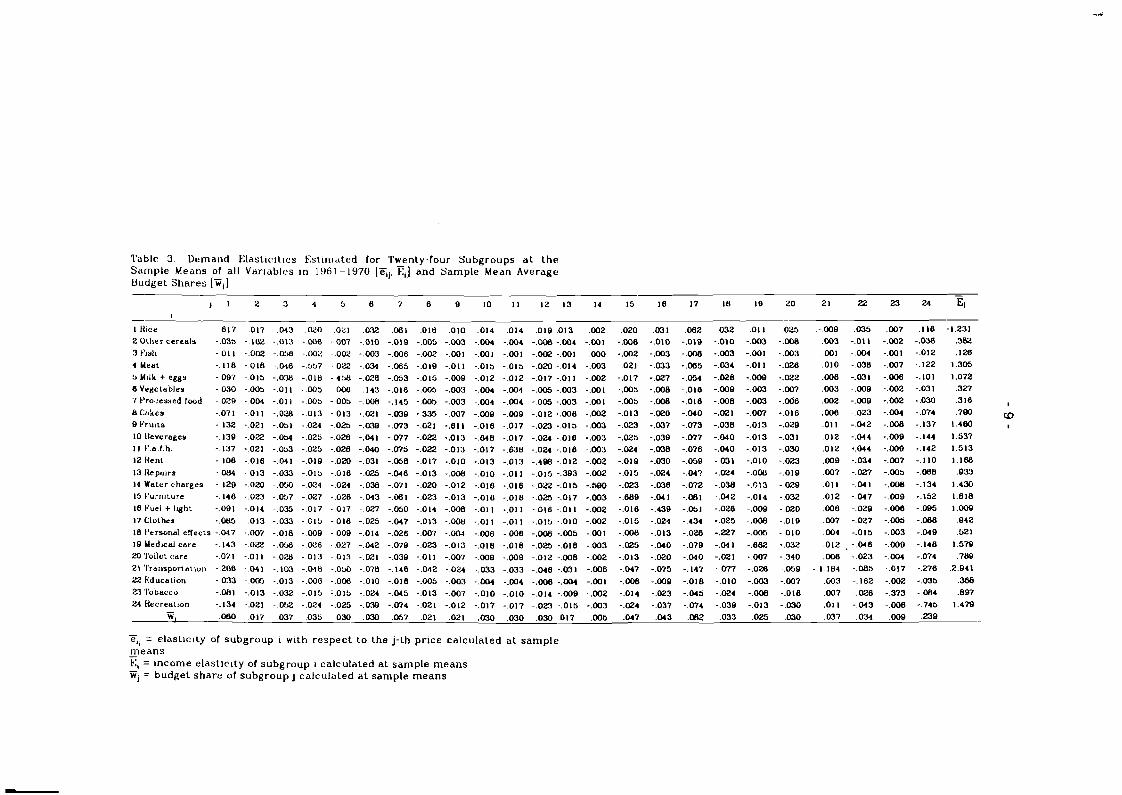
Table 3 Demand E l a s t ~ c ~ l ~ e s E s l ~ n ~ ~ r t e d for Twenty-four Subgroups a t the Sample Means of all Var~ables In 19611970 [Fl,. El] and Sample Mean Average Budge1 Shares IF,]

I liice 8 1 7 2 Other cereals -.035 3 Fish -.011

4 Meat -. I18 :3 Milk + egey -.007 6 Vegetables -.030 7 Pro.:ensed food -.OZQ M Cakes -.07 1 0 Frults -. 132 10 Deverages -. I30 I 1 F.8.f.h. - . 137 12 Rent -. I08

13 Repairs -.W I4 Water charges -. I20 15 E'url~~ture -. 148

18 Fuel + lylht -.001 17 Clothes -.065 18 t'trsonal etlects -.047 10 Uedlcal care - . I43 20 'l'oilet care -.071

21 'I'rar~sportatror~ -.208 22 Kduca~lon -.033 23 'I'obacco -.OM1 24 tiecreatlon -. 134 -

W, ,080

- e,, = elasL~c~Ly of subgroup i with respect Lo Lhe j-Lh price calculated a t sample means - El = income elast ic~ty of subgroup i calculated a t sample means - w, = budget share of subgroup j calculated a t sample means

Table 4. Dcmand Elastic~lies F:stirnaLed focTwenty-one Subgroups at the Sample Means of all Variables in 1963-19'17 [Zl,. El] and Sample Mean Average Budget Shares [Gi ]

1 Rlce ,033

2 Other cereals -.014 3 Fish -.008 4-5 Meat.

mik.etc . -.055 6 Vegetables -.032

7 Processed load -.022

8 Cakes -. 038 0 Fruits -.Of0

10 Heverages -.082 I 1 F.a.l . t~. -.Of8

12 Rent -.087

13 Repairs + water - ,036

I5 Fur l lure -.We 16 Fuel + light -.070 17 Clothir~g -.086

18 Personal eRects -.020

10 Medrcd care -.OD7

20 Toilet care -.a0

21 Transportation - . 154

22 Education .013

23-24 Tobacco + recrearjon -.080 -

W ,042

Zlj = elasticity of subgroup i with respect to the j-th price calculated at sample means - Ei = income elasticity of s~tbgroup i calculated at sample means - W, = budget share of subgroup j calculaled at sample means

also increased for cakes, fruits, rent, water charges, fuel and light, etc. Demand for transportation is highly responsive to a change in its price.

In the t h r d subperiod (Table 4) transportation, recreation, food away from home, medical care, and furniture are rather h g h in income elasticity, whle income elasticities of rent, fuel and light, clothes, etc., increased in comparison with the second subperiod.

It is apparent that the demand for subgroups of food commodities has become less elastic with respect to both income and own prlces over time. It is also notable that the housing demand as a whole has been substantially elastic during the entire period. More conspicuous is the fact that transportation has the largest income and own price elasticities, reflecting a strong demand for private cars in recent times.

5.3. Money Flexibilities From all the estimated linear expenditure sysJems, some good results were

chosen and their estimates of money flexibility w* were tabulated in Table 5. These estimates are liable to depend on the sample period, the level of commo- dity aggregation, and so on. However, they range from -2.0 to -2.5 without wide variations. Until comparatively recently, they tended to decline in absolute value. The corresponding x's and 9's were all estimated as statistically significant values.

Lastly, sample mean estimates of subsistence parameter pi were calculated, but they are not mentioned here. The concept of subsistence consumption lev- els are not applicable to inferior goods i.n an additive utility function. It is dis- cussed again with the economic implications of the dynamic model.

Table 5. Estimated Money Flexibility by the Sample Period and by the Commodity Classification (Static ~ o d e l )

6. EXPIRICAL RESULTS OF THE DYNAMIC MODEL

6.1. Estimates of Demand Parameters

Subperiod 195 1-60

1951-60 1959-73 1959-73 1960-72 1961 -70 196 1-73 196 1-73 1962-77

In estimation, equation (10) was used with alternative specifications of the proxy for changing tastes, as shown in equations (11) and (i2). It was fitted to longer time series of per capita expenditure and price data. Several favorable results were obtained from various data sets, whch are somewhat different in

Number of subgroups

2 1

22 23 2 4 24 24 2 3 24 2 1

2 1

Y

w* -2.455

-2.533 -2.401 -2.284 -2.547 -2.438 -2.295 -2.240 -1.957

Subgroups further aggregated Cakes and fruits, clothes and personal effects, tobacco and recreation Cakes and fruits, clothes and personal effects Meat, milk, etc.

Meat, milk, etc.

Meat, milk, etc, repairs and water, tobacco and recreation Meat, milk, etc, repairs and water, 1963-77 1 -2.221 ' tobacco and recreation

terms of sample period, proxy for taste variable, and commodity aggregation. One of the good results can be seen in Table 6. It reveals recent t rends in con- sumptlon patterns to some extent. The commodity classification is the same as in the thlrd subperiod (1963-77) in Table 1.

Table 6. Estimates of Demand Parameters Gi, Ci, xi in 1 9 5 8 - 1 977

Coefficient

i

1 Rice 2 Other cereals 3 Fish 4-5 Meat, milk, etc. 6 Vegetables 7 Processed food 8 Cakes 9 Fruits 10 Beverages 11 F.a.f.h. 12 Rent 13- 14 Repairs

+ water 15 Furniture 16 Fuel + light 17 Clothes 18 Personal effects 19 Medical care 20 Toilet care 2 1 Transportation 22 Education 23-24 Tobacco

Correlation coefficient

Coefficient of st variable

Serial correlation

coefficient

.575 ,322 .008

.804** ,508 ,493

,515 .578 ,522 .660** .376

.4 14

.514 ,393

,449 .702** .023 .654** .332

.832**

.568 + rec.

(Dynamic Model) Marginal budget

-.0205* -.0052* .0159*

.0278*

.0069*

.0116*

.0085*

.0197* ,0249.

-.0089* -.0046'

Taste variable st = mt - mt-A 'insignificant a t 5 percent (his ei, Ry.us) *+significant a t 5 percent (serial correlation coefficient)

share

Gi -.0540 .0032

-.0009

,0672 .0079 ,0205

,0151 ,0228 .0411

,0442 .0371

.0170

.0698

.0469

.0863 ,0166 ,0381 ,0205 ,1063

.0089

14 ratio

.750

.640 1.1 10

.766 ,484

1.081 . 1.001 1.218 1.596 .695 294

Estimated marginal budget shares are all significant except for fish. All subgroups other than rice and fish are defined to be normal goods. Significance of the coefficients of the taste variable turns out to be low on the whole. It would imply that changes in the quantities demanded of many subgroups are substan- tially explained by income and price changes withln the framework of economic theory. It is noteworthy, however, tha t the introduction of taste variable into the expenditure functions had a noticeable effect in stabilizing other relevant parameters in the regressions. The multiple correlation coefficients indirectly computed are very h g h ; on the other hacd, the serial correlation in the residu- als is not a serious problem in this case. Measures of fit in the total test a re mostly a t the level of 90 percent. These two facts indicate a high predictive power of the model. Only a couple of values of t h s measure are rather low, i.e., lor transportation in the early years of the period under consideration.

W ratio

22.003 4.322

.657

20.618 5.946

21.288

19.858 15.718 29.288 38.650 26.152

13.912 16.391 32.171

30.472 11.618 78.074

25.204 23.728

3.279

Table 7 1)emand E l a s t ~ c ~ l ~ e s F;sl~nialrd lor'l 'wenly-onr Subgroups a t the Sample Means of all Vdrldbles In 1950-19'77 IF,,. E,] and Sdniple Mean Average Budget Shares [i,]

] 1 2 3 4-5 8 7 8 10 11 12 13-14 15 18 17 18 18 20

4-S meat, milk, eLc. -.081

8 vegelables -.Om 7 processed

food - 028 8 cnkes -.OX3 Q fru~La -.087 10 beveraees - . l a I I f.a.1.h. - 103

12 rent -.OQl 1314 repaus

+ rater -.058

15 furrulure -.I 12

18 fuel + l ~ g h ~ -.OM 17 clothes -.OW I 8 personal

etTecLs -.040

10 med~cal care - 114 20 tollet care -.055 21 transporla-

tion -.I77 -.OX -.080 -.Of7 -.MI -.I08 -.032 -.023 - . a 8 -.Om -.034 -.034 -.08Q -.050 -.I02 -.058 -.020 -.045

22educat1on -.022 -.004 -.011 -.010 -.008 -.013 -.004 -.OX -.003 -.OM -.004 -.004 -.005 -.W -.013 -.007 -.003 -.006 2924 Lobacco

+ rec - -.I10 -.022 -.058 - . a 8 -.038 -.088 -.020 -.014 -.017 -.OlQ -.021 -.021 -.024 -.031 -.OM -.035 -.013 -.028

W, ,052 ,017 ,038 ,082 ,029 0.54 ,020 ,020 ,030 ,032 ,031 .022 ,047 ,042 ,081 ,031 ,025 ,028

- el, = e las t~c i ty of subgroup I w ~ t h respec t to the J-th pr ice calculated a t sample means - El = income elasticity of subgroup I calculated a t sample means - w, = budget share of subgroup J calculated a t sample means

6.2. Demand Elasticities Elasticities of demand with respect to deflated income and prices are given

in Table 7, evaluated at the sample means in the past 20 years. At first sight, Table 7 closely resembles Table 4 in the static model. There are only slight differences in income elasticities between the two tables. Education is now apparently a normal good. As regards the food category, beverages, food away from home, fruits, and meat are elastic with respect to income. In the nonfood category, transportation, medical care, furniture and recreation have very high income elasticities.

Own price elasticities in Table 7 are similar to those in Table 4. Ths implies that the money flexibility estimated by the dynamic model in 1958-77 is close to that of the static model in 1963-77. Estimated money flexibilities vary rather widely In the dynamic model, depending mainly on the length of sample period in t h s analysis. Nevertheless, . most of those estimates fell in the interval between -1 and -4.

6.3. Cost of Living Index and Subsistence Cost There are three exceptional subgroups in estimating the cost of living index

and the subsistence cost. They are rice, fish, and transportation. The first two subgroups have negative marginal budget shares, and the last one has a negative subsistence parameter. In disregard of their peculiarities, an attempt is made to estlmate the cost of living index and the subsistence cost. In fact, these three subgroups possess only small shares of the total budget. The calculation of the cost of living index follows the formula (see Hoa 1969a, 1969b, and Theil 1980).

cot = (I+?) ((CipitBiti CiPioBit) - ~ n i ( ~ i t / ~ i o ) 6i

(20)

where pit and pi, denote theLh price in the comparison and base periods respec- tlvely. The Bit can be obtalned by equation (13) after the estimates Ei, Ei, and h have been determined.

If the values of the cost of livlng index were all equal to 100, the General Consumer Price Index and the ' t rue' cost of living index would be the same. Though the values of the index in Table 8 are very close to 100, many of them do not attaln t h s level. I t would follow from the fact that the General Consumer Price Index in the Laspeyres form tends to have an upward bias as a deflator.

Cost of livlng index in 1958 = 100.0 Subsistence cost = zipidit

Table 8. Estimates of Cost of Living Index and Subsistence Cost by Year I Cost of

Year llving index 1958 / 100.0 1959 1 100.4 1960 100.3 196 1 100.0 1962 99.5 1963 99.1 1964 1 99.2 1965 1 98.3

Subsistence cost

122,120 122,25 1 122,080

1966 1967

98.6 98.7

Cost of Subsistence Year 1 living index cost

124,148 125,288 125,832 126,261 126,586 128,037 128,031 129,726 131,402 131,455

i968 1969 1970

98.8 99.1 99.1 99.5 99.5 99.3 99.3 99.5

100.0 100.2

122,159 , 1971 122,187 1 1972 122.520 1 1973 122,826 1 1974 123,014 1 1975 122,689 123,437

1976 1977

Estimated subsistence cost, as shown in Table 8, changes quite slowly over time. It results from the weak influence of the taste variable.

7. CONCLUDING REMARKS It was intended in this paper to systematically analyze the consumer

demand at subgroup levels on the basis of family budget data in 1951-77. All the commodities were classified into 21 to 24 subgroups in estimating the linear expenditure system. Powell's system was applied to the annual data In various segments of the whole period, estimating both static and dynamic parameters of the expenditure system.

The statlc model yielded well-defined demand relations and their charac- teristics in various subpe'riods, particularly in the three subperiods 1951-60, 1961-70, and 1963-77. Such a static approximation was attempted to preserve the linearity of expenditure functions and to take account of the possible changes in preferences during the whole period. Evidently from the empirical results, price and income elasticities of demand have changed over time, and the values of money flexibility show a little variation in dependence on sample period, commodity classification and so on.

In the dynamic model, many of the estimated parameters for the taste vari- able were not statistically significant, but some important demand and utility parameters were obtained. Estimates of money flexibility were fairly change- able according to the income level, specification of the taste variable and so on. They were more or less different from those of the static model. Price elastici- ties in the dynamic model are also a t variance with the static results. The strik- ing features of the results are that the measures of fit of the model were very hlgh In interpolation test, and that the estimated parameters were rather stable as a whole.

Consumer demand estimation in more recent years will be discussed on another occasion.

NOTES

1. Let the cross substitution term in the Slutsky equation be K i j Then the sym- metry condition is

KIj = A(axi/ am) (ax,/ am), ( i # j ) , (A: constant)

2. The A is related to Theil's income flexibility p and to Frisch's money flexibility L as follows:

V

( A / m) = -(P = -(I / w ) , (m: income)

Frisch's money flexibility ; is equivalent to the income elasticity of the marginal ut-ility of income. Since the supernumerary ratio is defined as (see Coldberger 1970):

A 1s interpreted as the supernumerary income in the linear expenditure system.

3. Denote the substitution term by Kij. Then zit is of the form:

zit = (pit/ A)CjKi j(~j t /Fj)

4. The maximum likelihood method entails a greater burden of computation as compared with the least squares method. As regards the convergence of demand parameters in nonlinear regressions, the maximum likelihood method appears to involve some difficulty. Lluch and Powell (1975) and Lluch and Williams (1975) reported the results that maximum likelihood estimates did not converge in some cases, but that convergence was acheved in those cases by the least squares method in the estimation of the linear expenditure system and of the extended linear expenditure sys- tem, respectively.

5 . Assume that X and y are the matrix and vector whose elements consist of sample data on exogenous variables. Furthermore, if we assume in regard to the error structure that there is no serial correlation either withn or across equations, and that there is no contemporaneous correlation across equations but: a common error variance for all equations, maximum likeli- hood method reduces to least squares method (see Goldgberger and Camaletsos 1970, Lluch and Williams 1975). The error structure in t h s case is of the form

j and t = t ' ) , E(& i t& jO = ~ ' o ~ ~ r w i s e

However, t h s error specification is practically implausible, as was pointed out by Goldberger and Gamaletsos (1970).

6. The simple assumption is that there is no serial correlation either withn or across equat~ons and that there is no contemporaneous correlation across equations but a constant error variance for each equation. The error specification in t h s case is of the form

(.f (i = j and t = tp) , E('lt'rt') = 0 otherwise

7. The variances of the estimators Si and h under least squares postulates are mentioned below:

o& = a?/ Ctuf . (i = 1.2 ,.... N)

of = (CiDi -u:) . Ctu?/ ( C i ~ i ) 2

aiZ indicates the error variance in the estimating equation for the com- modity, and its unbiased estimator ordinarily takes the expression

@i2 = C e$/ (T - 2)

with eit being the residual and ( T - 2) the degree of freedom. 8. For the theoretical features of Leser's system, see Sasaki and Saegusa 1974.

9. The criterion of convergence is written as below, denoting the estimate X in round r by xr(r = 1,2,.. .):

The variances of estimators Gi, c?, and x are

of is the error variance of theTh equation, and its unbiased estimator is

ai2 = Cei2/ (T - 3), (ei: residual)

rii ( i = 1,2) indicates a diagonal element in the inverse matrix:

In t h s paper, the sample size is not reduced by taking differences in annual income for the specification of the taste variable.

11. For details on data, see Sasaki (1981). 12. The static model of Leser's system is expressed as

vi = piYi + E(Vi C j p ~ - piYi) + bi(m - CjpjYj)

It does not require an iterative estimation. The taste variable st is added to the above equation to extend ~t to a dynamic model in this analysis.

13. The multiple correlation coefficient R was computed as the simple correla- tion coefficient between actual and estimated expenditures for each sub- group.

14. The measure of fit in the total test IS the ratio of calculated expenditure Vit to actual expenditure vit. Thls is equivalent to taking the ratio of calculated quantity consumed per capita Sit to its actual value Xi t .

Measure of fit = ( V i t / vit) = (;it/ xit)

REFERENCES

Goldberger, A.S., and T. Gamaletsos. 1970. A Cross-Country Comparison of Con- sumer Expenditure Patterns. European Economic Review 1:357-400. Spring 1970.

Hoa, T.V. 1969a. Additive Preferences and Cost of Living Indexes: an Empirical Study of the Australian Consumer's Welfare. The Economic Record 45:432- 440, September, 1969.

Hoa, T.V. 1969b. Consumer Demand and Welfare Indexes: a Comparative Study for the United Kingdom and kustralia. Economica 36:409-425, November, 1969.

Leser, C.E.V. 1960. Demand Functions for Nine Commodity Groups in Australia. Australian Journal of Statistics 2: 102-1 13, November, 1960.

Leser, C.E.V. 1961. Commodity Group Expenditure Functions for the United Kingdom, 1948-1957. Econometrica 29:2G-32, January, 1961.

Lluch, C . , and A. Powell. 1975. International Comparisons of Expenditure Pat- terns. European Economic Review 5:275-303, July, 1975.

Lluch, C. , and R. Williams. 1975. Cross Country Demand and Savings Patterns: an Application of the Extended Linear Expenditure System. Review of Economics and Statistics 57:320-328, August, 1975.

Onish, H. 1980. A Mathematical Framework for the Japanese Agricultural Model. WP-00-156. Laxenburg, Austria: International Institute for Applied Systems Analysis.

K.S. Parikh, F. Rabar, editors. 1981. Food for All in a Sustainable World: The IIASA Food and Agriculture Program. SR-81-002. Laxenburg, Austria: Inter- national Institute for Applied Systems Analysis.

Powell, A.A. 1966. A Complete System of Consumer Demand Equations for the Australian Economy Fitted by a Model of Additive Preferences. Econome- trica 34:661-675, July, 1966.

Powell, A.A., T.V. Hoa, and R.H. Wilson. 1968. A Multi-Sectoral Analysis of Consu- mer Dem.and in the Post-War Period. Southern Economic Journal 35: 109- 120, October, 1968.

Sasaki, K. 1981. Sengo no Shohisha Juyotaikei no Keisoku. (On the Measurement of the Consumer Demand Systems in the Postwar Period.) Annual Report 1980. The Japan Committee for IIASA.

Sasaki, K. , and Y. Saegusa. 1974. Food Demand Matrix in an Approximate Linear Expenditure System. American Journal of Agricultural Economics 56:263- 270, May, 1974.

Stone, J . R . N . 1954. Linear Expenditure Systems and Demand Analysis: an Appli- cation to the Pattern of British Demand. Economic Journal 64:511-527, Sep- tember, 1954.

Theil, H. 1980. The System-Wide Approach to Microeconomics. Ch. 3. Chicago: The University of Chicago Press.