1

ESTIMATION OF THE MAIN THERMAL CHARACTERISTICS OF BUILDING COMPONENTS USING PARAMETRIC MODELS

IN MATLAB

M. J. JIMÉNEZ1, H. MADSEN2, K. K. ANDERSEN2

1 CIEMAT, Department of Energy, Energy Efficiency in Buildings Unit, Av. Complutense 22, E-28040, Madrid, Spain, e-mail: mjose.jimenez@psa.es

2 Informatics and Mathematical Modelling, Technical University of Denmark, Building 321, DK - 2800 Lyngby – Denmark

ABSTRACT This paper presents the application of IDENT Graphical User Interface of MATLAB to estimate the thermal properties of building components from outdoors dynamic testing, imposing appropriate physical constraints and assuming linear and time invariant parametric models. Theory is briefly described to provide the background for a first understanding of the used models. The relationship between commonly used RC-network models and the parametric models proposed is deduced. The analysis is generalised for different possibilities in the assignment of inputs and outputs and even multi-output. A step by step guidance illustrated by an example is included. Results obtained using the different possibilities in selecting inputs and outputs are reported. Keywords: Building energy, Thermal parameters, Outdoors testing, System identification 1. INTRODUCTION Thermal modelling of buildings has important applications such as designing control strategies and estimating parameters characterising the system. The latter is of special importance when the parameters of interest have physical meaning, i.e. the estimates reflect physical quantities such as resistances, capacities and time constants of the building. There exist a variety of tools for estimating parameters of buildings (Gutschker, 2000), (Kristensen et al., 2003), etc. These tools differ in applied estimation method, user interface and foremost what kind of model types can be applied. Most of these tools are based on deterministic differential equations or state space models. The purpose of this paper is to describe how the Matlab System Identification (IDENT) toolbox (Ljung, 1999), together with appropriate physical constraints, can be used to estimate such physical parameters. The IDENT toolbox allows for estimation of very general ARMAX models. This model class is often associated with black-box models and have traditionally been used in prediction, simulation and control applications but very few references report its use to estimate thermal parameters of building components. This paper demonstrates how the model parameters can be given physical interpretation by comparing the ARMAX models with equivalent physical models. Furthermore, the IDENT toolbox allows for both, estimation of simulation and prediction based models, the former being the most commonly used method within thermal modelling for simulation purposes, whereas the latter should be applied whenever the values of physical parameters are of interest. The paper is organized as follows. First, a mathematical description of linear and time invariant models is given. A special case of this model class is the ARMAX model (Box and Jenkins, 1976), which can be used for estimating physical parameters of thermal systems. Then, in Section 3, we describe how classical RC-networks of thermal systems, which are derived based on first principles, can be formulated as ARMAX models. Subsequently, we describe how the parameters of the resulting ARMAX model can be given a physical interpretation. The method is illustrated by considering a simple RC network model for the heat dynamics of a wall. Section 4, briefly describes the two different estimation methods, the output error method and the prediction error method. The former is relevant when the model is intended for simulation purposes, whereas the latter is relevant for control (or prediction) purposes, or when the physical parameters are of interest, e.g. in fault detection and diagnosis. Section 6 gives a brief discussion on validation methods, an integral part of model building.

2

In section 7 some guidelines are presented, which illustrates some of the possibilities within IDENT to identify and estimate ARMAX models. Subsequently, a case study is presented in section 8. Finally, a conclusion with discussion is given. 2. LINEAR AND TIME-INVARIANT (LTI) MODELS This section gives a mathematical description of linear and time-invariant models. Let us consider systems with input and output signals, often called input-output systems. Let us further limit our attention to causal linear and time-invariant systems (RC-networks are an example of linear and time-invariant systems). The models in IDENT toolbox belong to the family of linear and time-invariant models. 2.1. Non-parametric models Time domain For linear and time-invariant systems there exists a function called the impulse response function hk, which describes the relationship between the input signal ut and the output signal yt. For causal single-input-single-output (SISO) systems the relationship is described by the folding sum1:

∑∞

=−=

0kktkt uhy (1)

Using the back-shift operator2, defined by q-1yt = yt-1, and a generalized operator function h(q) (often called the transfer function):

.....)( 22

110 +++= −− qhqhhqh (2)

the relationship between input and output can be written as

tt uqhy )(= (3) In practice, some deviations between h(q)ut and the measured output yt must be seen. These deviations are described by introducing a noise term Nt, i.e.

ttt Nuqhy += )( (4) The noise term Nt is in general autocorrelated noise. In the multiple-input-multiple-output (MIMO) case h(q) is a matrix containing the individual scalar impulse response functions between the corresponding elements of the vectors ut and yt. Using the summation operator S(q)=(1 + q-1 + q-2 + .....) the step response function Sk is easily obtained from the impulse response function:

kk hqSS )(= (5) The impulse response function acts as the most flexible description of linear time-invariant systems (lumped parameter models are a subset of such systems). Steady state relations between input ut and output yt are obtained by putting q=1, which is equivalent to consider yt and ut as constants.

1 Notation in this document assumes sampling interval as one time unit, which simplifies notation without loosing generality. For example in eq. (1) if the sampling interval is Δt then ut-k should be replaced by ut-kΔt. 2 If the sampling interval is Δt, then the back-shift operator is defined by q-1yt = yt-Δt.

3

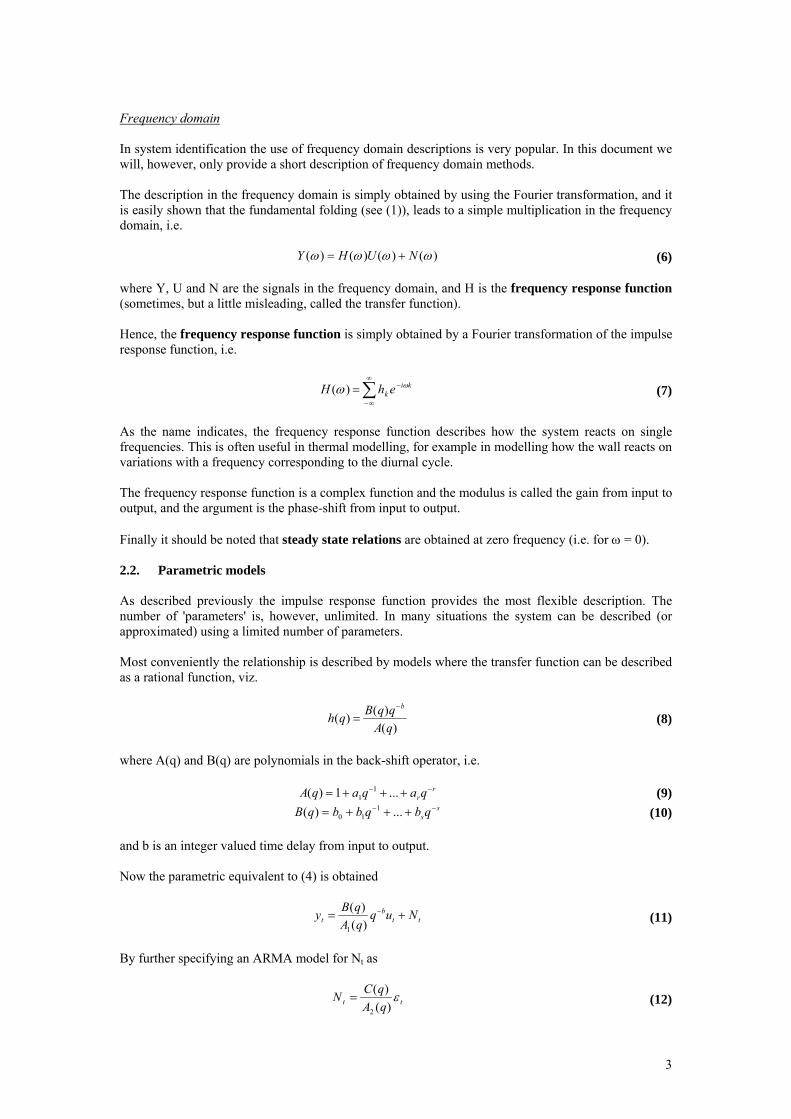
Frequency domain In system identification the use of frequency domain descriptions is very popular. In this document we will, however, only provide a short description of frequency domain methods. The description in the frequency domain is simply obtained by using the Fourier transformation, and it is easily shown that the fundamental folding (see (1)), leads to a simple multiplication in the frequency domain, i.e.

)()()()( ωωωω NUHY += (6) where Y, U and N are the signals in the frequency domain, and H is the frequency response function (sometimes, but a little misleading, called the transfer function). Hence, the frequency response function is simply obtained by a Fourier transformation of the impulse response function, i.e.

∑∞

∞−

−= kik ehH ωω )( (7)

As the name indicates, the frequency response function describes how the system reacts on single frequencies. This is often useful in thermal modelling, for example in modelling how the wall reacts on variations with a frequency corresponding to the diurnal cycle. The frequency response function is a complex function and the modulus is called the gain from input to output, and the argument is the phase-shift from input to output. Finally it should be noted that steady state relations are obtained at zero frequency (i.e. for ω = 0). 2.2. Parametric models As described previously the impulse response function provides the most flexible description. The number of 'parameters' is, however, unlimited. In many situations the system can be described (or approximated) using a limited number of parameters. Most conveniently the relationship is described by models where the transfer function can be described as a rational function, viz.

)()()(qAqqBqh

b−

= (8)

where A(q) and B(q) are polynomials in the back-shift operator, i.e.

rrqaqaqA −− +++= ...1)( 1

1 (9) s

sqbqbbqB −− +++= ...)( 110 (10)

and b is an integer valued time delay from input to output. Now the parametric equivalent to (4) is obtained

ttb

t NuqqAqBy += −

)()(

1

(11)

By further specifying an ARMA model for Nt as

tt qAqCN ε

)()(

2

= (12)

4

where εt is a sequence of uncorrelated random variables (a white noise process) and C(q) is a polynomial in the back-shift operator, we obtain the Box-Jenkins transfer function model

ttb

t qAqCuq

qAqBy ε

)()(

)()(

21

+= − (13)

The term B(q)q-b/A1(q) is called the transfer function component. In modelling we often assume A1(q) = A2(q) = A(q). Hereby we obtain the ARMAX-model (AutoRegressive-Moving Average with eXogeneous input)

tbtt qCuqByqA ε)()()( += − (14)

where A(q), B(q) and C(q) are p'th, s'th and q'th order polynomials, respectively, in the shift operator q. Special cases of the ARMAX model is the ARX-model (C(q)=1) and FIR (Finite Impulse Response) (A2(q)=C(q)=1). The ARMAX model is sometimes referred to as the CARMA model (Controlled ARMA). An Output Error Model (OE model) is a model on the form

tbtt NuqAqBy += −)(

)( (15)

where there is no model for the noise term. The models are most often applied in estimation by the Output Error Method (OEM). This will be elaborated in the section on estimation. It is straightforward to extend the model to the case of multiple inputs, and relatively straightforward also to the multiple input -multiple output case. 3. FROM RC-NETWORK TO ARMAX MODELS In this section it will be shown how physical linear models on state space forms can be formulated as ARMAX models. The link between state space and ARMAX models will be demonstrated. Consider a wall mounted in a test cell for outdoor testing as sketched in (Figure 1). The wall consists of an outer wall, an insulating part and an inner wall represented as thermal network model (Figure 2).

Outdoors

Te

Wall

gGv

U(Ti-Te)Q

Solar radiation

Test room

TiOutdoors

Te

Wall

gGv

U(Ti-Te)Q

Solar radiation

Test room

Ti

Figure 1. Scheme of wall installed in a PASSYS

test cell and main heat fluxes crossing it.

H1 H2

C1 C2 gGv QTe

TiT2T1H3H1H1 H2H2

C1 C2 gGv QTe

TiT2T1H3H3

Figure 2. A simple RC network model for the

heat dynamics of a wall. Te is the outside temperature, Ti is the inside temperature, Q is the heat flux density through the wall (measured on the inner surface), and Gv is the global solar irradiance on the outdoor surface of the wall. The heat interchange through the wall is induced by the temperature difference between indoors and outdoors and by the solar irradiance incident on the outdoor surface (See Figure 1). The thermal characteristics of the wall governing the heat flux rate crossing it, are the heat transmission coefficient U and the solar energy transmittance g, verifying the following steady state equation:

5

( ) vei gGTTUQ −−= (16) For dynamic conditions the heat capacitance C, should also be considered. We use a simple dynamical model for the temperature variations of the wall to estimate the heat conductance and heat capacitance of the various components of the wall. The RC diagram shown in Figure 2 represents a frequently used model for this kind of walls. H1, H2 and H3 are the heat conductance corresponding to the outer wall, the insulating part and the inner wall respectively. C1 and C2 are the heat capacitance of the outer wall and the inner wall, T1 and T2 are the temperature of the outer wall and the inner wall. (Hi and Ci are here considered per unit area). U can be obtained taking into account that 1/U=1/H1+1/H2+1/H3. For this system different possibilities for selecting the output (or response variable) exist. Some analysis techniques applied for this type of tests were reported in (SIC 1, 1994) and (SIC 2, 1996). Most traditional approaches used either the inside temperature Ti or the heat flux density Q as output variable. In general it is obvious to use both as output variables. The possibilities for arrangement of inputs and outputs, using single-output and multi-output models, are mentioned in the following. 3.1. Using Q as output variable Using a sloppy notation for the noise processes, the dynamic state space model for this system can be written as:

( ) ( )dt

dTTHTTHdt

dTC e1

122111

1ω

+−+−= (17)

( ) ( )dt

dTTHTTH

dtdT

C i2

232122

2ω

+−+−= (18)

( ) eTTHQ i +−= 23 ; ( )2,0 qNe σ∈ (19) We measure three variables, namely Te, Ti and Q, with measurement errors, which are presented in the dynamic equations as (dω1,dω2)T and e, respectively. e is a white noise process, while ω1 and ω2 are two independent Wiener processes with incremental standard deviations σ1 and σ2. Rearranging terms in (17) to (19) leads to:

( )

( )⎥⎦

⎤⎢⎣

⎡+⎥

⎦

⎤⎢⎣

⎡

⎥⎥⎥⎥

⎦

⎤

⎢⎢⎢⎢

⎣

⎡

+⎥⎦

⎤⎢⎣

⎡

⎥⎥⎥⎥

⎦

⎤

⎢⎢⎢⎢

⎣

⎡

+−

+−=⎥

⎦

⎤⎢⎣

⎡

2

1

2

3

1

1

2

1

3222

2

1

221

1

2

1

0

0

1

1

ωω

dd

dtTT

CH

CH

dtTT

HHCC

HCHHH

CdTdT

i

e (20)

( ) eTTHQ i +−= 23 ; ( )2,0 QNe σ∈ (21) Introducing aij and bij to simplify notation and considering only the deterministic part of the state space model (20) it is seen that it can be written as:

dtTT

bb

dtTT

aaaa

dTdT

i

e⎥⎦

⎤⎢⎣

⎡⎥⎦

⎤⎢⎣

⎡+⎥

⎦

⎤⎢⎣

⎡⎥⎦

⎤⎢⎣

⎡−

−=⎥

⎦

⎤⎢⎣

⎡

22

11

2

1

2221

1211

2

1

00 (22)

Taking the Laplace transform we obtain:

⎥⎦

⎤⎢⎣

⎡⎥⎦

⎤⎢⎣

⎡=⎥

⎦

⎤⎢⎣

⎡⎥⎦

⎤⎢⎣

⎡+−−+

i

e

TT

bb

TT

asaaas

22

11

2

1

2221

1211

00 (23)

and by isolating T1 and T2:

6

( )( )

ATT

asbbabaasb

TT i

e

det11221121

22122211

2

1⎥⎦

⎤⎢⎣

⎡⎥⎦

⎤⎢⎣

⎡+

+

=⎥⎦

⎤⎢⎣

⎡ (24)

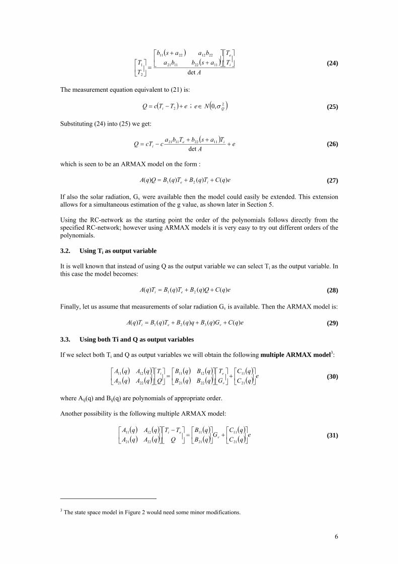
The measurement equation equivalent to (21) is:

( ) eTTcQ i +−= 2 ; ( )2,0 QNe σ∈ (25) Substituting (24) into (25) we get:

( )e

ATasbTba

ccTQ iei +

++−=

det11221121 (26)

which is seen to be an ARMAX model on the form :

eqCTqBTqBQqA ie )()()()( 21 ++= (27) If also the solar radiation, Gv were available then the model could easily be extended. This extension allows for a simultaneous estimation of the g value, as shown later in Section 5. Using the RC-network as the starting point the order of the polynomials follows directly from the specified RC-network; however using ARMAX models it is very easy to try out different orders of the polynomials. 3.2. Using Ti as output variable It is well known that instead of using Q as the output variable we can select Ti as the output variable. In this case the model becomes:

eqCQqBTqBTqA ei )()()()( 21 ++= (28) Finally, let us assume that measurements of solar radiation Gv is available. Then the ARMAX model is:

eqCGqBqqBTqBTqA vei )()()()()( 321 +++= (29) 3.3. Using both Ti and Q as output variables If we select both Ti and Q as output variables we will obtain the following multiple ARMAX model3:

( ) ( )( ) ( )

( ) ( )( ) ( )

( )( ) eqCqC

GT

qBqBqBqB

QT

qAqAqAqA

v

ei⎥⎦

⎤⎢⎣

⎡+⎥

⎦

⎤⎢⎣

⎡⎥⎦

⎤⎢⎣

⎡=⎥

⎦

⎤⎢⎣

⎡⎥⎦

⎤⎢⎣

⎡

21

11

2221

1211

2221

1211 (30)

where Aij(q) and Bij(q) are polynomials of appropriate order. Another possibility is the following multiple ARMAX model:

( ) ( )( ) ( )

( )( )

( )( ) eqCqC

GqBqB

QTT

qAqAqAqA

vei

⎥⎦

⎤⎢⎣

⎡+⎥

⎦

⎤⎢⎣

⎡=⎥

⎦

⎤⎢⎣

⎡ −⎥⎦

⎤⎢⎣

⎡

21

11

21

11

2221

1211 (31)

3 The state space model in Figure 2 would need some minor modifications.

7

4. ESTIMATION METHODS In this paper only the Output Error Method - OEM and the Prediction Error Method - PEM will be described briefly. In the literature a lot of other methods can be found. In Matlab/Ident both OEM and PEM methods are provided. PEM has been used later on in this work. 4.1. Output error method By applying the Output Error Method we consider the Output Error Model and the unknown parameters (denoted θ) are estimated by:

( ) ( )⎭⎬⎫

⎩⎨⎧

== ∑=

N

ttNS

1

2minargˆ θθθθ

(32)

Where:

( ) tb

tt uqqAqByN −−=

)()(

1

θ (33)

Nt(θ) is the simulation error, since it represents the deviation between yt and the simulated output from the model. The covariance matrix for the parameter estimates is often very difficult to calculate using the output error method. Furthermore, the most common validation techniques cannot be applied, e.g. test for white noise and normally distributed residuals. Therefore, the method should only be used under special conditions. 4.2. Prediction error methods The prediction error estimate is found by minimising the sum of the squared prediction errors:

( ) ( )⎭⎬⎫

⎩⎨⎧

== ∑=

N

ttS

1

2minargˆ θεθθθ

(34)

Where:

( ) )(ˆ1/ θθε −−= tttt YY (35)

is the one-step prediction errors or residuals. If the predictions are calculated using the correct model, then the one-step prediction error becomes a white noise sequence. Using various tests for white noise this enables a powerful possibility for model validation. For this method the covariance matrix for the parameters estimates are readily obtained. Furthermore, the method provides an estimation of a model for the errors. The parameters belonging to the C-polynomial can be used, for instance, to obtain an error decomposition; more precisely the total error can be composed into measurement error and model error. This fact enables a powerful tool for model evaluation. 5. OBTAINING THE PHYSICAL PARAMETERS We do now have the theory available for illustrating how to obtain the physical parameters using ARMAX models. In Section 3 it is shown how to obtain an ARMAX model from a specified RC-network model (or state space model) as traditionally used for identification of the heat dynamics of building components.

8

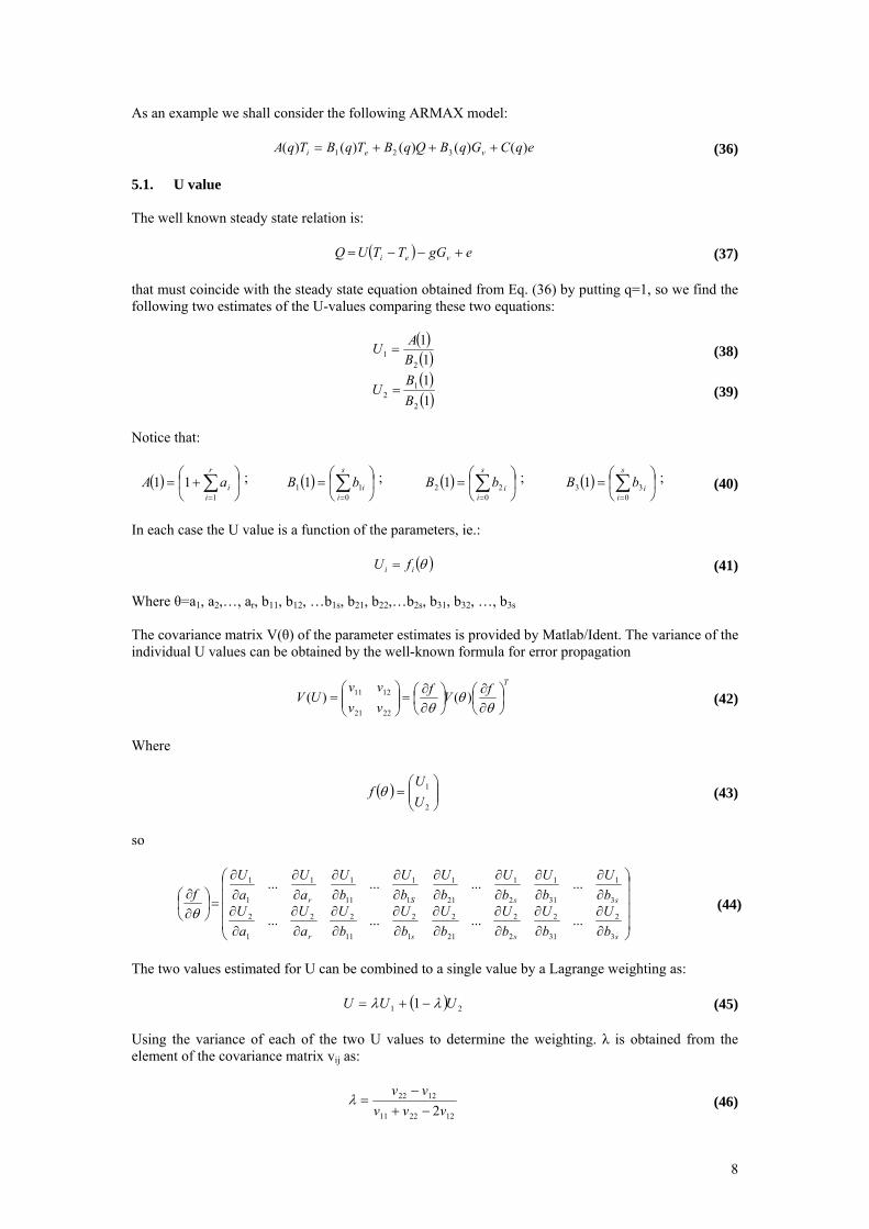
As an example we shall consider the following ARMAX model:

eqCGqBQqBTqBTqA vei )()()()()( 321 +++= (36) 5.1. U value The well known steady state relation is:

( ) egGTTUQ vei +−−= (37) that must coincide with the steady state equation obtained from Eq. (36) by putting q=1, so we find the following two estimates of the U-values comparing these two equations:

( )( )11

21 B

AU = (38)

( )( )11

2

12 B

BU = (39)

Notice that:

( ) ⎟⎠

⎞⎜⎝

⎛ += ∑=

r

iiaA

1

11 ; ( ) ⎟⎠

⎞⎜⎝

⎛= ∑=

s

iibB

011 1 ; ( ) ⎟

⎠

⎞⎜⎝

⎛= ∑=

s

iibB

022 1 ; ( ) ⎟

⎠

⎞⎜⎝

⎛= ∑=

s

iibB

033 1 ; (40)

In each case the U value is a function of the parameters, ie.:

( )θii fU = (41) Where θ=a1, a2,…, ar, b11, b12, …b1s, b21, b22,…b2s, b31, b32, …, b3s The covariance matrix V(θ) of the parameter estimates is provided by Matlab/Ident. The variance of the individual U values can be obtained by the well-known formula for error propagation

TfVfvvvv

UV ⎟⎠⎞

⎜⎝⎛∂∂

⎟⎠⎞

⎜⎝⎛∂∂

=⎟⎟⎠

⎞⎜⎜⎝

⎛=

θθ

θ)()(

2221

1211 (42)

Where

( ) ⎟⎟⎠

⎞⎜⎜⎝

⎛=

2

1

UU

f θ (43)

so

⎟⎟⎟⎟

⎠

⎞

⎜⎜⎜⎜

⎝

⎛

∂∂

∂∂

∂∂

∂∂

∂∂

∂∂

∂∂

∂∂

∂∂

∂∂

∂∂

∂∂

∂∂

∂∂

∂∂

∂∂

=⎟⎠⎞

⎜⎝⎛∂∂

sssr

ssSr

bU

bU

bU

bU

bU

bU

aU

aU

bU

bU

bU

bU

bU

bU

aU

aU

f

3

2

31

2

2

2

21

2

1

2

11

22

1

2

3

1

31

1

2

1

21

1

1

1

11

11

1

1

............

............

θ

(44)

The two values estimated for U can be combined to a single value by a Lagrange weighting as:

( ) 21 1 UUU λλ −+= (45) Using the variance of each of the two U values to determine the weighting. λ is obtained from the element of the covariance matrix vij as:

122211

1222

2vvvvv−+

−=λ (46)

9

And the corresponding standard deviation as the square root of its variance as:

( )122211

2122211

*2*

vvvvvvU

−+−

=σ (47)

5.2. g value The g value is determined as:

( )( )11

2

3

BB

g = (48)

and the variance of the estimate is again calculated by using the variance propagation approach, as described above. 5.3. Time constants The time constants are related to the A-polynomial. The number of time constants is equal to the order of the A-polynomial. Assuming that the order of the A-polynomial is r then the polynomial A(q) has r roots. For each root pi the corresponding time constant τi is calculated as

( )ii pln

1=τ (49)

5.4. Impulse and step response functions For each combination of inputs and outputs an impulse response function can be found. The impulse response function is simply found by a polynomial division of the relevant polynomials of the ARMAX model. For instance the impulse response function from the solar radiation to the indoor air temperature is calculated as

( )( )qAqBqh 3)( = (50)

and the step response function is then found by a summation of the impulse response function, as described by (5). 6. MODEL VALIDATION When building a dynamic model it is important that certain criteria for the model fit are met to ensure an adequate model. Several procedures for model validation exist (see Madsen, 2001). Here we shall only list the following criteria for model determination and validation suggested by Norlén (1994):

1. Fit to the data. The model residuals should be 'small' and 'white noise'. A necessary condition for 'white noise' is that there should be neither autocorrelation in the residuals nor correlation between the residuals and the input variables.

2. Internal validity. The model should agree with data other than data used for parameter

estimation (cross validation). 3. External validity. The result from the model should not (without greater motivation) conflict

with previous experiences or other known conditions.

10

4. Dynamic stability. From a steady state, the model should give an output upon a temporary change in an input variable that is gradually faded out (if the model is intended to describe dynamic characteristics).

5. Identifiably. It should be possible to determine the parameters of the model uniquely from the

data. 6. Simplicity. The model should be as small as possible.

7. GUIDELINES FOR USING MATLAB/IDENT IN THE PROPOSED APPROACH In this section directions for using the Matlab IDENT toolbox to apply the modelling approach proposed in the previous sections will be given. The steps are illustrated in Section 8.5 to estimate the U-value for an opaque wall component. The GUI of IDENT is used to examine data, and to fit and validate the proposed ARMAX model. There exist a variety of possibilities within IDENT which are useful for building and examining the model. However, the discussion is limited to the most crucial steps. Before IDENT can be started it is necessary to start Matlab, to load the dataset into Matlab and to start IDENT by typing ident in the Matlab prompt. (It is useful to give abbreviated names for the columns to be used into the model as for example the same nomenclature used for the corresponding physical quantities Ti, Te, Q and Gv in the Matlab prompt). After starting IDENT, the main menu of the GUI in IDENT appears as shown in Figure 3.

Figure 3. The GUI of IDENT. Then working data must be loaded, by clicking on data and then import. A new window will appear that allows specifying these data as the corresponding columns or using the names given to each column. After loading the data the main screen is seen as in Figure 4. Notice that the imported data appear in bold fonts, meaning that it is active. If you work with several dataset at the same time only the data in bold fonts will be active. The data can be viewed by clicking the Time plot, and something like Figure 5 is obtained. Notice, that from within the time plot window, there are several possibilities to modify and customize the plot, e.g. to check other input against the output.

11

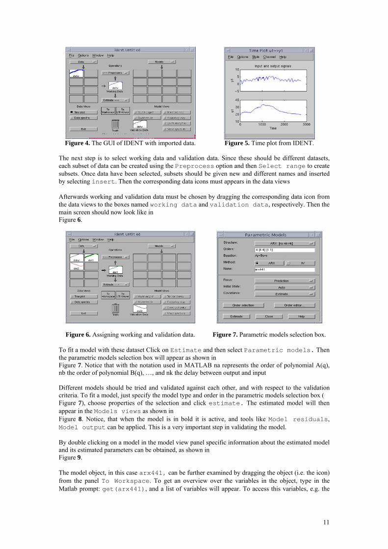
Figure 4. The GUI of IDENT with imported data. Figure 5. Time plot from IDENT.

The next step is to select working data and validation data. Since these should be different datasets, each subset of data can be created using the Preprocess option and then Select range to create subsets. Once data have been selected, subsets should be given new and different names and inserted by selecting insert. Then the corresponding data icons must appears in the data views Afterwards working and validation data must be chosen by dragging the corresponding data icon from the data views to the boxes named working data and validation data, respectively. Then the main screen should now look like in Figure 6.

Figure 6. Assigning working and validation data.

Figure 7. Parametric models selection box. To fit a model with these dataset Click on Estimate and then select Parametric models. Then the parametric models selection box will appear as shown in Figure 7. Notice that with the notation used in MATLAB na represents the order of polynomial A(q), nb the order of polynomial B(q), …, and nk the delay between output and input Different models should be tried and validated against each other, and with respect to the validation criteria. To fit a model, just specify the model type and order in the parametric models selection box ( Figure 7), choose properties of the selection and click estimate. The estimated model will then appear in the Models views as shown in Figure 8. Notice, that when the model is in bold it is active, and tools like Model residuals, Model output can be applied. This is a very important step in validating the model. By double clicking on a model in the model view panel specific information about the estimated model and its estimated parameters can be obtained, as shown in Figure 9. The model object, in this case arx441, can be further examined by dragging the object (i.e. the icon) from the panel To Workspace. To get an overview over the variables in the object, type in the Matlab prompt: get(arx441), and a list of variables will appear. To access this variables, e.g. the

12

parameter vector, type arx441.ParameterVector. To access the uncertainty of the parameter estimates, type arx441.CovarianceMatrix. To access the roots type roots(arx441.a) Now having the individual estimated parameters and its uncertainty, the U value, g value, time constants and their corresponding uncertainties are obtained as explained in Sections 5.1, 5.2 and 5.3, respectively. Matlab M-files (programs) could be used for these calculations.

Figure 8. The models view.

Figure 9. Specific information from model estimation.

The step response function and the impulse response function can easily be calculated by clicking on the panel in Ident. Also the frequency response function is quickly obtained by the clicking on the panel. As very important tools for model validation the autocorrelation functions and the cross correlation functions are readily calculated by clicking on the panel in Ident. 8. CASE STUDY 8.1. Objective of the test The objective of this test is to estimate the U value of the opaque component, described below, from an outdoor dynamic test. These tests are part of round robin tests carried out in several European PASLINK test sites (Baker and Strachan, 2003). The mentioned reference also provides a lot of additional and useful information for external validation. 8.2. Tested component The analysed component is a quite simple homogeneous and opaque wall. It consists of a sandwich of insulation between plywood, and the following materials have been used for its construction: • 200mm thick of expanded polystyrene (PS30), density 30kg/m3, consisting in 4 layers 50mm thick. • Phenolic plywood of 12 mm thick. • White melamine 0.7mm thick for outdoor face. • Sikaflex 11FC has been used to glue layers. • 16 Nylon bolt+washers+nuts size M12, uniformly distributed, to give consistency to the

construction. A more detailed description can be found in (Baker and Strachan, 2003). 8.3. Test procedure The component has been tested installed in a real size test cell. Figure 1 represents a scheme of the main heat interchanges through the wall once the component has been installed in the test cell. The following sensors have been used for measurements; ventilated and protected from direct solar

13

radiation PT100 for air temperatures, pyranometer (Kipp&Zonen CM11) for solar irradiance on the component surface, and thermopile based transducers (PU 32 manufactured at TNO) for heat flux density. Tests have been carried out according the PASLINK typical test. This procedure consists in a test sequence including 3 days of low power, 1.5 days of high power and 3.5 days according to a ROBLS power sequence. The maximum power levels depend on the weather conditions of the test site. 8.4. Data The following data, corresponding to the described opaque component tested at different test sites with the same test procedure, have been analysed: • Data set nº1: Data analysed corresponding to the component tested at BRE (Glasgow, Scotland).

These data are available in www.paslink.org. • Data set nº2: Data from the experiments on the component tested at CIEMAT (Almería, Spain).

This experiment was carried out in the period 6th of January to 24th of January, 2002.

-100

100

300

500

700

900

1100

14 16 18 20 22 24 26 28 30 32 34 36 38Time (Days)

Gv (

W/m

2 )

Gv

Figure 10. Global solar irradiance on the outdoors wall

surface. Data set nº2.

0

5

10

15

20

25

30

35

40

14 16 18 20 22 24 26 28 30 32 34 36 38Time (Days)

Tem

pera

ture

(°C

)

Te Ti

Figure 11. Indoors and outdoors air temperatures. Data set nº2.

0

1

2

3

4

5

6

7

14 16 18 20 22 24 26 28 30 32 34 36 38Time (Days)

Hea

t flu

x de

nsity

(W/m

2 )

Q

Figure 12. Heat flux density leaving the test room measured

in the indoors surface of the component. Data set nº2.

8.5. Example of estimation of U and g values This section describes “step by step” the estimation of U and g, using IDENT in MATLAB, for data set nº1. Only ARX models have been considered to simplify the analysis without loss of generality. The following types of models have been considered as candidate model to estimate U and g: • Models including Gv as input. In this case the small value of g can be determined. • Models that not include Gv, which suppose the value of g as negligible and obviously cannot be

determined by these models. • Single output models. • Multi-output models. Section 8.6 summarises the obtained results for each of the considered models. As only steady state parameters are required, only plots of residuals, average of residuals and estimated identification errors have been considered in order to compare the performance of the models. In this section an ARX model using Ti as output and Te, Q and Gv as inputs, as described in Section 3.2, has been considered as an example to illustrate how to obtain the U and g values. IDENT in MATLAB has been used to select model structure and order, and also to generate the matrix containing information about the selected model structure, estimated parameters and their estimated accuracy, as described in Section 7. The study has been limited to models with, na, nb and nk, varying between 1 and 10. The models pointed as “Best Fit” are those where orders are na=10, nb=[10 10 10] and nk= [1 1 1]. The results of these estimations are presented in Figure 13.

14

Figure 13. Results of model selection, using Te, Q and Gv as inputs, and Ti as output.

In this case “Best Fit” models have been selected and used to estimate the required parameters.

1 2 3 4 5 6 7x 1 0 5

1 6

1 8

2 0

2 2

2 4

2 6

2 8

T i m e ( s )

Tem

pera

ture

(ºC

)

m e a s u r e d o u tp u t 1 s t e p p r e d i c t e d o u t p u t

Figure 14. Measurements and predicted outputs

given by the “Best Fit” models versus time.

Figure 15. Residual given by the “Best Fit”

models versus time. The average of the residuals is 0.0002 ºC.

Figure 16. Residual autocorrelation and cross-correlation.

15

The matrix containing information about the selected model structure has been exported to MATLAB workspace, once in the workspace, the required parameters and their estimation errors have been obtained from this matrix. The table bellow presents the identified parameters for the selected ARX model. Table 1. Identified parameters for an ARX model with na=10, nb=[10 10 10] and nk=[1 1 1].

ia ib1 ib2 ib3 i=1 -5.98E-01 -1.95E-03 7.83E-02 3.13E-05i=2 -3.00E-01 5.53E-03 -5.18E-02 -6.46E-07i=3 -2.45E-01 -3.64E-03 8.17E-03 -1.19E-05i=4 -6.80E-02 1.16E-03 2.35E-02 -2.13E-05i=5 -1.53E-02 -6.33E-04 -2.82E-02 8.03E-06i=6 4.75E-02 3.80E-03 -6.65E-03 2.69E-06i=7 1.70E-02 -3.68E-03 1.37E-02 5.83E-06i=8 5.77E-02 -3.70E-03 -2.22E-02 2.97E-05i=9 4.63E-02 4.73E-03 1.08E-02 -1.29E-06i=10 6.01E-02 1.23E-03 -1.09E-02 6.54E-06

By using (38) to (48) the values in Table 2 are obtained: Table 2. Physical parameters.

Parameter Estimate Units U1 = 1.86E-01 ± 3.46E-03 W/m2K U2 = 1.94E-01 ± 1.37E-02 W/m2K g = 3.32E-03 ± 7.05E-04 -

And finally applying Lagrage’s method and rounding the result according to the obtained errors the following values are obtained: Table 3. Results.

Parameter Estimate Units U = 0.191 ± 0.009 W/m2K g = 0.0033 ± 0.0007 -

Afterwards the model has been validated using the validation criteria described in Section 6 as follows: Figure 14 shows good fit between measured and predicted output, and Figure 15 and Figure 16 show low and uncorrelated residuals. External validity is guaranteed as these results agree with the results obtained for the same component tested through the same test procedure in other test sites and also with values estimated from tabulated values. It has dynamic stability otherwise a warning message would appear in MATLAB command window after having estimated the parameters. The identifiably of the model is obvious. And finally its simplicity is acceptable. So it is concluded that this model fits the validation criteria presented in Section 6. 8.6. Summary of results given by different models Several models have been tried in both cases and those giving the best results are summarised in Table 4 and 5 for data set nº1 and nº2, respectively.

16

Table 4. Results obtained for the data set nº1 using all data for identification and validation: U and g.

Model

Number Inputs Outputs Model U

(W/m2K) error_U

(W/m2K) g

(-) error_g

(-) 1 Q Ti-Te arx10101(BF) 0.19 0.03 N/A N/A 2 Q,Gv Ti-Te arx10101(BF) 0.21 0.03 0.02 0.01 3 Te,Q,Gv Ti arx10101(BF) 0.191 0.009 0.0033 0.0007 4 Te,Q Ti arx10101(BF) 0.20 0.01 N/A N/A 5 Gv Ti-Te,q arx221 0.178 0.007 0.001 0.001

Table 5. Results obtained for data set nº2. (The first 2/3 of data file has been used for identification

and the last 1/3 for validation): U and g.

Model Number

Inputs Outputs Models U (W/m2K)

error_U (W/m2K)

g (-)

error_g (-)

1 Q Ti-Te arx882(BF) 0.173 0.006 N/A N/A 2 Q,Gv Ti-Te arx461(AIC) 0.180 0.009 0.0008 0.0007 3 Ti-Te Q arx2107(MDL,AIC,BF) 0.176 0.004 N/A N/A 4 Ti-Te,Gv Q arx225(BF) 0.191 0.003 0.0020 0.0002 5 Ti,Te,Gv Q arx136(MDL,AIC,BF) 0.197 0.005 0.0029 0.0003 6 Gv Ti-Te,q arx111 0.193 0.003 0.0023 0.0002

In both cases the estimated g is too low and its estimated error is too high as expected for an opaque component. Notice the low identification error (Table 4 and Table 5) and low average of residuals (Figure 17 to Figure 20) obtained when a two outputs model is considered.

Figure 17. Residual given by the single output model number 2 of Table 5, versus time. The

average of the residuals is –0.01065 ºC.

Figure 18. Residual given by the single output model number 4 of Table 5, versus time. The

average of the residuals is -0.007 W/m2.

Figure 19. Residual given by the two outputs model number 6 of Table 5, versus time. The

average of the residuals is 0.0002 ºC.

Figure 20. Residual given by the two outputs model number 6 of Table 5, versus time. The

average of the residuals is 0.003 ºC W/m2.

17

9. CONCLUSIONS In this paper a procedure for using IDENT in MATLAB for estimating the thermal characteristics of a wall component is suggested. The flexibility of this approach has been demonstrated by the use of several models with different assignment of inputs and outputs and even multi-outputs models. Very good performance has been found for multi-output models giving very low identification errors. A different analysis tool (eg. CTSM, Kristensen and Madsen, 2003) must be applied for those components where non linear effects were relevant. NOMENCLATURE

Symbol Quantity Units U: Heat transmission coefficient Wm-2K-1 g: Solar energy transmittance φ : Heat flux through the building component. W Q : Heat flux density. Wm-2 Gv : Vertical global irradiance Wm-2 Ti : Indoors air temperature °C Te : Outdoors air temperature °C ΔT Temperature difference between indoors and outdoors air. °C A Area of the tested building component m2

REFERENCES Andersen, K. K.; Madsen, H.; Hansen L. 2000. Modelling the Heat Dynamics of a Building using

Stochastic Differential Equations. Energy and Buildings 31:13-24. Baker, P.; Strachan, P. 2003. WP3 Round Robin Tests as Feasibility Study for Standardization. Final

Technical Report Part 3. IQ-TEST Project, Contract nº ERK6-CT1999-2003. Box, G. E. P.; Jenkins, J. M. 1976. Time Series Analysis: Forecasting and Control. San Francisco,

USA: Holden-Day. Gutschker, O. 2000. LORD User Manual. PASLINK EEIG, www.paslink.org Kristensen, N.R.; Madsen, H. 2003. Continuous Time Stochastic Modelling – CTSM 2.3 User Guide.

Technical University of Denmark , Lyngby, Denmark. www.imm.dtu.dk/ctsm Kristensen, N.R.; Madsen, H.; Jørgensen, S.B. 2004. Parameter Estimation in Stochastic Grey-Box

Models. Automatica. 40: 225-237. Kristensen, N.R.; Madsen, H.; Jørgensen, S.B. An Investigation of some Tools for Process Model

Identification for Prediction, Accepted for publication in (Ed.) A.S. Asprey and S. Macchietto: Dynamics Model Development: Methods, Theory and Application, Elsevier, 2003.

Ljung, L. 1999. System Identification. Theory for the User. New Jersey: Prentice Hall. Norlén, U. 1994. Determining the Thermal Resistance from In-Situ Measurements. In: Workshop on

Application of System Identification in Energy Savings in Buildings (Edited by Bloem, J.J.), 402-429. Published by the Commission of The European Communities DG XIII, Luxembourg.

Nielsen, J.N.; Madsen, H.; Young, P.C. 2000. Parameter Estimation in Stochastic Differential Equations; An Overview. Annual Reviews in Control. 24: 83-94.

Nielsen, B.; Madsen, H. 1998. Identification of a Continuous Time Linear Model of the Heat Dynamics in a Greenhouse. J. Agric. Engng. Res. 71:249-256,.

Madsen, H. 2001. Time Series Analysis. Institute of Mathematical Modelling, Technical University of Denmark, Lyngby, Denmark.

Madsen, H.; Holst, J. 1995. Estimation of Continuous-Time Models for the Heat Dynamics of a Building. Energy and Buildin. 22:67-79.

SIC 1. 1994. Workshop on Application of System Identification in Energy Savings in Buildings. Edited by J.J. Bloem, Published by the Commission of the European Communities, L-2920 Luxembourg, Ref.: EUR 15566 EN

SIC 2. 1996. System Identification Competition. Edited by J.J. Bloem, Published by the Office for Official Publications of the European Communities, L-2985 Luxembourg, Ref.: EUR 16359 EN, ISBN 92-827-6348-X