estimation of vector error correction … ·...
TRANSCRIPT

ESTIMATION OF VECTOR ERROR CORRECTION MODEL WITH GARCH ERRORS: MONTE CARLO SIMULATION AND APPLICATION Koichi Maekawa* Hiroshima University of Economics [email protected] Kusdhianto Setiawan# Faculty of Economics and Business Universitas Gadjah Mada [email protected] ABSTRACT The standard vector error correction (VEC) model assumes the iid normal distribution of disturbance term in the model. This paper extends this assumption to include GARCH process. We call this model as VEC-‐GARCH model. However as the number of parameters in a VEC-‐GARCH model is large, the maximum likelihood (ML) method is computationally demanding. To overcome these computational difficulties, this paper searches for alternative estimation methods and compares them by Monte Carlo simulation. As a result a feasible generalized least square (FGLS) estimator shows comparable performance to ML estimator. Furthermore an empirical study is presented to see the applicability of the FGLS. Presented on INTERNATIONAL CONFERENCE ON ECONOMIC MODELING – ECOMOD 2014 Bali, July 16-‐18, 2014 This manuscript consists of two parts. On Part I we developed the estimation method and on Part II we applied the new method for testing international CAPM. (*) the author of part I of this manuscript (#) the co-‐author of part I and author of part II of this manuscript, presenter of the paper in the conference
2
PART I
ESTIMATION METHOD DEVELOPMENT
1. INTRODUCTION
Vector Error correction (VEC) model is often used in econometric analysis and estimated
by maximum likelihood (ML) method under the normality assumption. ML estimator is
known as the most efficient estimator under the iid normality assumption. However there
are disadvantages such that the normality assumption is often violated in real date,
especially in financial time series, and that ML estimation is computationally demanding
for a large model. Furthermore in our experience of empirical study error terns in VEC
model often show a GARCH phenomenon, which violates iid assumption. To overcome
these disadvantages and to reduce computational burden of ML estimator it may be
worthwhile to reconsider the feasible generalized least square (FGLS) estimator instead
of ML estimator (MLE) because FGLS method is relatively free from the distributional
assumptions and ease computational burden.
The purpose of this paper is to examine the finite sample properties of FGLS estimator in
VEC-GARCH model by Monte Carlo simulation and by real data analysis of the
international financial time series. The paper is organized as follows: Section 2 briefly
surveys the multivariate GARCH (MGARCH hereafter) model; Section 3 describes VEC
representation of the vector autoregressive (VAR) model; Section 4 presents a VEC-
GARCH model and shows that this model can be estimated by FGLS within the
framework of the seemingly unrelated regression (SUR) model; Section 5 examines the
performance of FGLS by Monte Carlo simulation; Section 6 presents an empirical
application of VEC-GARCH model and shows the applicability of FGLS; finally Section
7 gives some concluding remarks.

3
2. MULTIVARIATE GARCH
Multivariate GARCH model has been developed and applied in financial econometrics
and numerous literature were published. The recent development in this area were
surveyed by Bauwens, L., S. Laurent and J. V. K. Rombouts (2006) and T. Ter svirta
(2009) . Before investigating MGARCH model in this paper we briefly introduce
MGARCH model focusing on relevant MGARCH models in our study.
2.1. vech-GARCH model
The univariate GARCH model has been generalized to N-variable multivariate GARCH
models in many ways. The most straightforward generalization is the following vech-
GARCH model by Bollerslev, Engle, and Woodridge (1988):
( ) , ( ) (1)
where ( ) , and is assumed to follows a multivariate normal
distribution ( ). An element of the variance covariance matrix is denoted by
: [ ] In the most general vech-GARCH model ( ) is given by
( ) ∑ (
) ∑ ( ) (2)
where ( ) is an operator that vectorizes a symmetric matrix. We briefly illustrate the
2-variable case (N=2) for simplicity. For N=2 and p=q=1 ( ) is written as follows:
(
) ( )
,
and c is an (N(N+1)/2)×1=3×1 vector, and and are N(N+1)/2×N(N+1)/2 =3×3
parameter matrices. Then ( ) is written as
[
]

4
[
] [
] [
] [
] [
] (3)
or
This representation is very general and flexible but there is a disadvantage that only a
sufficient condition for the positive definiteness of the matrix is known. Furthermore
the number of parameters is ( )( ( ) ) ( ) which is large unless
N is small. For example, if and , the number of parameters is 21, if N=3
it is 78. This may cause computational difficulties.
2.2. Diagonal vech model
To reduce such disadvantages mentioned above Bollerslev, Engle, and Wooldridge
(1988) proposed diagonal vech model in which the coefficient matrices and are
assumed diagonal. In this case the number of parameters is reduced to (
) ( ) ). For example, if and then the number is 9, and if N=3
it is 8. Furthermore, in this case the necessary and sufficient conditions for the positive
definiteness of are obtained by Bollerslev, Engle, and Nelson (1994). The variance
equation (3) is simplified as follows:
[
] [
] [
] [
] [
] [
]
or

5
2.3. BEKK model
To ensure the positive definiteness of Engle and Kroner (1995) proposed a
following model called as Baba-Engle-Kraft-Kroner (BEKK) model.
∑ ∑
∑ ∑
(4)
where are N×N coefficient matrices, C is a lower triangular matrix. Although
this decomposition of the constant term can ensure the positive definiteness of , which
is the advantage of this model, the number of parameters is quite large. Because of this,
estimation of this model is often infeasible for a large model. When K=1 this model is
written as
(5)
In this case the number of parameters is np ( ) ( ) . If
and N=2, then , and for N=3. If it may not be feasible to
estimate this model. To reduce number of parameters it is common and popular to
assume that the coefficient matrices A, B are diagonal. This model is called Diagonal
BEKK model (Engle and Kroner (1995)). In this model np=( ) ( ) . If
and N=2, then , and for N=3. For small size Diagonal BEKK
model the calculation is feasible. However, even in Diagonal BEKK model, np will be
large when N is not small. For example, np=35 when and N=5.
We illustrate several versions of (5) for a simple case N=2 and K=1:
Unrestricted BEKK. In this case the variance covariance matrix [
] is
expressed as
[
] [
] [
]
[
] [
]
[
]
[
]

6
or
( )
( )
where is positive definite by construction.
Diagonal BEKK is expressed as
[
] [
] [
]
[
] [
]
[
]
[
]
or
where in these variance covariance equations only depend on their own lagged
values .
Engle and Kroner (1995) shows that the diagonal vech and the diagonal BEKK are
equivalent as follows: By stacking the diagonal elements of A and B of the diagonal vech
model, i.e.,
( ) ( )
and write
then it is easy to see that ( ) is identical to the diagonal vech.
There are many other types of multivariate GARCH model. They are surveyed, for
example, in Bauwens, L., S. Laurent and J. V. K. Rombouts (2006) and Silvennoinen and
Terasvirta (2009).

7
Bollerslev, Engle, and Wooldridge (1988) introduced a restricted version of the general
multivariate vec model of GARCH with following representation:
where the operator is the Hadamard product and is Kronecker Product. To ensure
the positive semi-definiteness (PSD) there are several ways for specifying coefficient
matrices. One example is to specify , , and B as products of Cholesky factorized
triangular matrices. Such parameterization will be used in the latter section in this paper.
2.4. Log-likelihood function of vech-GARCH
If the distribution of errors is a multivariate normal, then the log-likelihood function of
(1) is given by
∑ ( )
∑ | |
∑
(6)
In calculating MLE we have to invert at every time t. This is computationally tedious
when T and N are not small. Furthermore is often noninvertible.
3. VEC REPRESENTATION OF VAR MODEL
We consider M-variate and k-th order vector autoregressive time series
=[ ]
(7)
This model is called Vector Autoregressive (VAR) Model. The subscript t denotes time:
. The errors are assumed to follows iid M-dimensional multivariate
normal distribution N(0, ). Note that does not depend on time t. Later in this paper we
consider the time dependent case, i.e., . Now by introducing a matrix defined
by
We can rewrite (7) as
(8)
8
where,
= [ ] a vector of first order lagged of .
= [ ] : a vector of first difference of at time t.
C0 =
: a vector of constant terms.
= : a vector of disturbance errors which is assumed iid M-dimensional
multivariate normal distribution N(0, ).
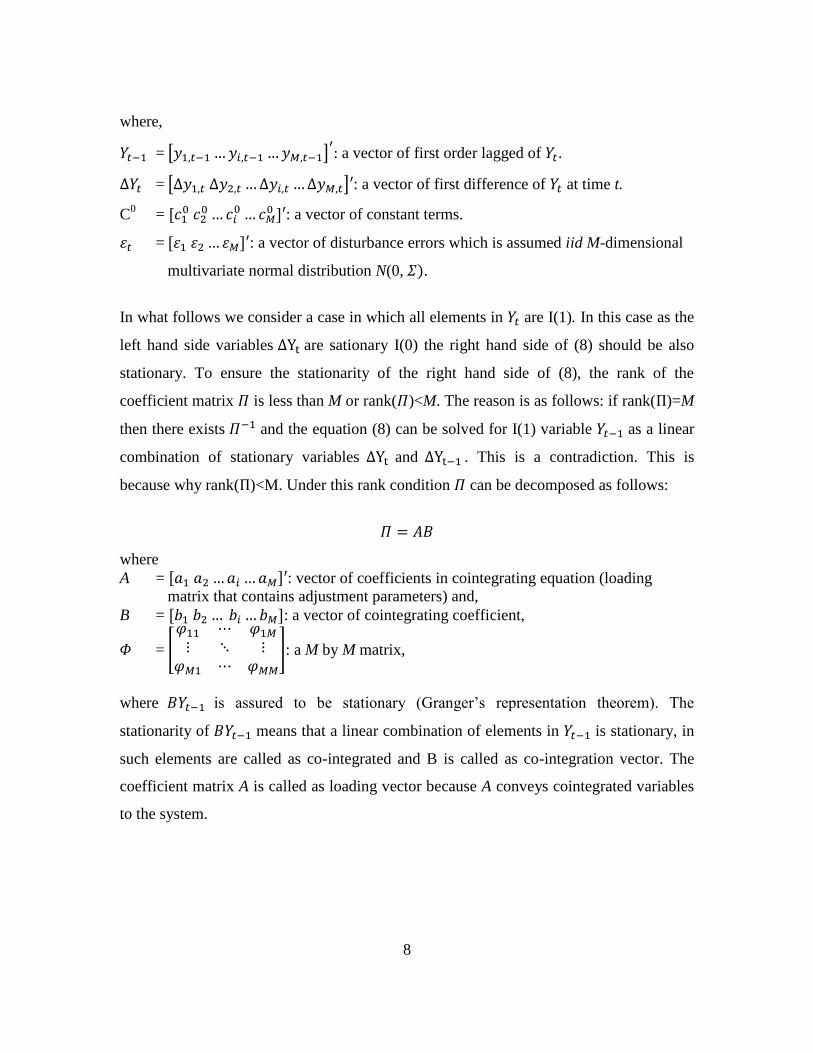
In what follows we consider a case in which all elements in are I(1). In this case as the
left hand side variables are sationary I(0) the right hand side of (8) should be also
stationary. To ensure the stationarity of the right hand side of (8), the rank of the
coefficient matrix is less than M or rank( )<M. The reason is as follows: if rank( )=M
then there exists and the equation (8) can be solved for I(1) variable as a linear
combination of stationary variables and . This is a contradiction. This is
because why rank( )<M. Under this rank condition can be decomposed as follows:
where
A = : vector of coefficients in cointegrating equation (loading
matrix that contains adjustment parameters) and,
B = : a vector of cointegrating coefficient,
= [
]: a M by M matrix,
where is assured to be stationary (Granger‟s representation theorem). The
stationarity of means that a linear combination of elements in is stationary, in
such elements are called as co-integrated and B is called as co-integration vector. The
coefficient matrix A is called as loading vector because A conveys cointegrated variables
to the system.

9
4. VECTOR ERROR CORRECTION WITH GARCH ERRORS (VEC-GARCH
MODEL)
4.1. VECM with BEKK errors
So far we have considered the standard Vector Error Correction Model (VECM), where a
set of time series is nonstationary at level, but stationary at their first differences and
( ) Matrix represents the long run relationship between the variables in
Equation (8) and Johansen (1988) proposed a maximum likelihood estimation of (8) for
the case of the rank of matrix , where .
In what follows, we relaxed the assumption of homoscedasticity of the errors. Instead, we
assume that has zero mean and time dependent variance-covariance matrix of that
has the BEKK GARCH structure as given by (6):
4.2. SUR representation
VEC model with GARCH errors can be represented by Seemingly Unrelated Regression
(SUR) model as follows. SUR representation of VEC model seems to be worthwhile to
consider. For simplicity we consider three-equation VEC model such as:
or
[
] [
] [
] [
] [
] [
]
for t=1, 2, …, n.
Alternatively this system can be written as
(9)
where and are the ith row of and respectively, i.e.,

10
[
] [
] [
] [
]
(
) (
)
and,
.
Defining new matrices X and by
and
,
the 3-equation VEC model (8) can be written as SUR model as follows:
[
] [
] [
].
We assume that ( ) , ( ) for , and the variance and covariance
( ) and ( ) follow MGARCH(1,1). Let us define ( ), or in
the complete form:
[
]
where, is a n×n diagonal matrix where its main diagonal elements are elements of n-
vector of and zeros on the off diagonal elements and, , i.e.,
[
]
11
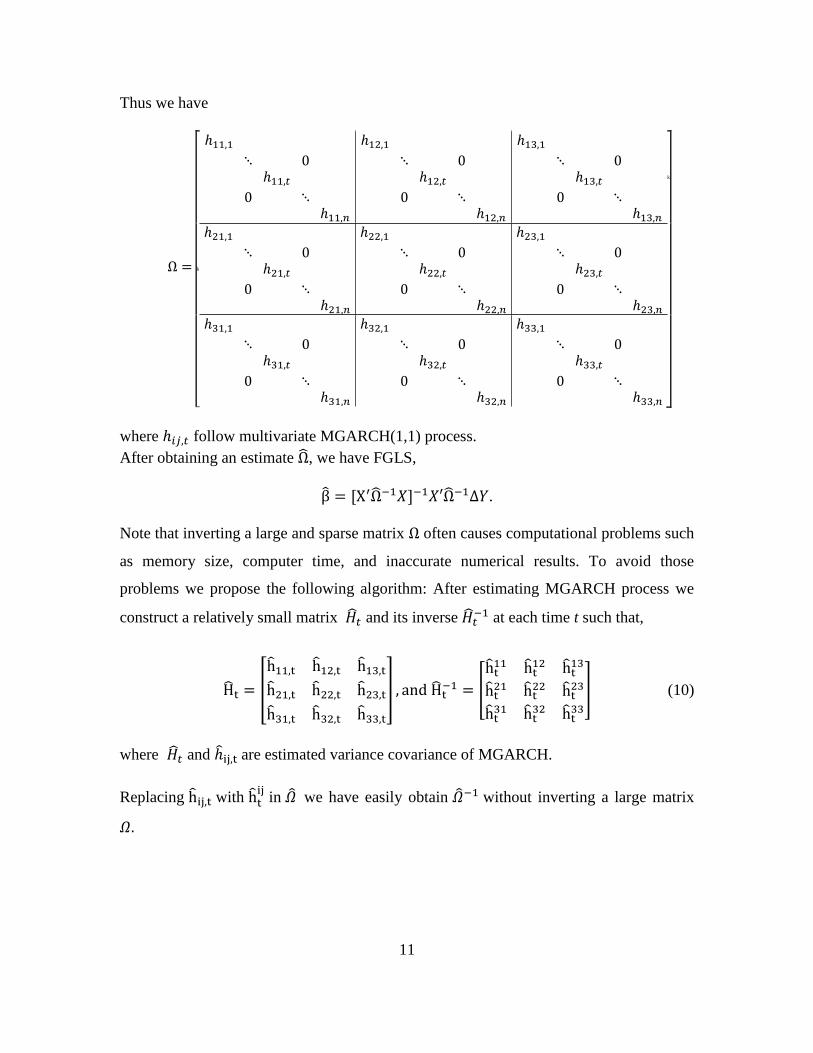
Thus we have
k
k
where follow multivariate MGARCH(1,1) process.
After obtaining an estimate , we have FGLS,
.
Note that inverting a large and sparse matrix often causes computational problems such
as memory size, computer time, and inaccurate numerical results. To avoid those
problems we propose the following algorithm: After estimating MGARCH process we
construct a relatively small matrix and its inverse at each time t such that,
[
] [
] (10)
where and are estimated variance covariance of MGARCH.
Replacing with in we have easily obtain without inverting a large matrix
12
5. MONTE CARLO SIMULATION
5.1 Data generating Process (DGP)
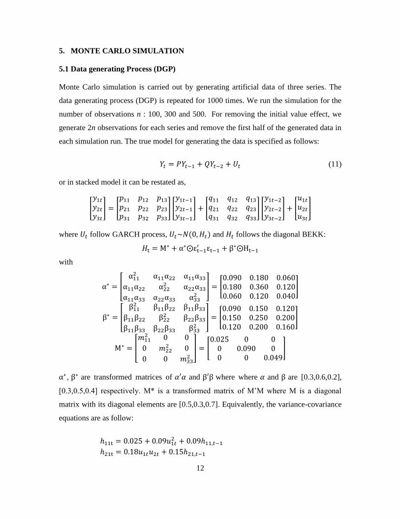
Monte Carlo simulation is carried out by generating artificial data of three series. The
data generating process (DGP) is repeated for 1000 times. We run the simulation for the
number of observations n : 100, 300 and 500. For removing the initial value effect, we
generate 2n observations for each series and remove the first half of the generated data in
each simulation run. The true model for generating the data is specified as follows:
(11)
or in stacked model it can be restated as,
[
] [
] [
] [
] [
] [
]
where follow GARCH process, ( ) and follows the diagonal BEKK:
with
[
] [
]
[
] [
]
[
] [
]
, are transformed matrices of and where where and are [0.3,0.6,0.2],
[0.3,0.5,0.4] respectively. M* is a transformed matrix of M‟M where M is a diagonal
matrix with its diagonal elements are [0.5,0.3,0.7]. Equivalently, the variance-covariance
equations are as follow:
13
Equation (11) can be rewritten as Vector Error Correction Model (VECM):
(12)
where and . The true values of P and Q are set as follow:
[
] and [
]
thus [
] which can be decomposed into loading vector and
cointegrating vector .
Before we generate , we have to generate ~N(0, ) as follows.
Step 1. Generate [
] ( )
Step 2. Generate using Diagonal BEKK model from
Step 3. Transform to by applying Cholesky Decomposition: , where
is lower triangular matrix obtained from decomposing .
By construction, the positive definiteness (PD) of is assured.
5.2. Estimation Strategy
Under the above DGP we carried out Monte Carlo simulation for the following five
cases:
Case 1 (OLS): We estimate parameters equation by equation in equation (9) by OLS
without considering GARCH error structure and obtain the followings:

14
Case 2 (VECM): We estimate parameters in equation (12) by VECM system equation
without considering GARCH error structure and obtain the followings:
Case 3 (FGLS-OLS-GARCH/FOLSH): First we calculate OLS residuals for each
equations without considering GARCH error structure as in Case 1. Next, we use for
obtaining variance covariance matrix and in the diagonal BEKK model. Having
and in hand we can construct and to have feasible generalized least square
(FGLS) estimator.
Case 4 (FGLS-VECM-GARCH/FVECH): We use VECM system equations as in Case
2 for estimating . First we obtain each residual from VECM in Case 2. Next, we use
for obtaining variance covariance matrix and in the diagonal BEKK model.
Having and in hand we can construct and to have feasible generalized
least squre (FGLS) estimator.
Case 5 (MLE): We estimate all parameters in the mean equation (12) and the diagonal
BEKK variance equation (5) by MLE and obtain the estimated system as follows:
Mean equation:
Variance equation:
or equivalently the variance-covariance equations are as follow:
In estimating the parameters we maximize log likelihood function as specified in
Equation (6). We run the simulation in Eviews program (version 7.2). For Case 5, in
15
order to starting the iteration, the initial values of VECM parameters (the mean equation)
were set based on single OLS equations as in Case 1. Meanwhile, the initial values for
MGARCH parameters in the variance equations were set based on univariate GARCH.
5.2. Simulation Results
The main estimation methods under investigation in this paper are FGLS-based estimator
(FOLSH and FVECH) and Maximum Likelihood Estimator (MLE). These strategies are
taking into account the presence of MGARCH error structure. Presumably, the strategies
are expected to outperform the other strategies that neglect the MGARCH error structure
(OLS and VECM). Summary of simulation results is presented in Table 1. From the
table, we observed that estimation methods FOLSH, FVECH, and MLE seem to
outperform the other methods (OLS and VECM); the mean of the estimated parameter
from 1000 times simulation run tends to be closer to its true value in most cases.

16
Table 1: Parameter Estimates from Monte Carlo Simulation n=100
True Value
OLS VECM FOLSH FVECH MLE
Parameters Mean Std.Dev. Mean Std.Dev. Mean Std.Dev. Mean Std.Dev. Mean Std.Dev.
0.000 -0.048 0.082 -0.011 0.074 -0.043 0.082 -0.042 0.081 -0.038 0.078
0.000 -0.010 0.083 -0.011 0.074 -0.008 0.083 -0.008 0.084 -0.007 0.079
0.000 0.005 0.040 0.005 0.037 0.003 0.040 0.003 0.040 0.003 0.037
-0.300 -0.272 0.127 -0.279 0.127 -0.275 0.129 -0.275 0.131 -0.282 0.122
0.000 -0.001 0.082 0.018 0.132 -0.002 0.085 -0.001 0.084 -0.002 0.079
0.000 0.001 0.049 -0.520 0.149 0.001 0.052 0.001 0.050 0.001 0.048
0.000 -0.017 0.099 -0.019 0.090 -0.009 0.092 -0.009 0.094 -0.010 0.076
0.000 -0.072 0.109 -0.020 0.091 -0.051 0.098 -0.047 0.102 -0.040 0.084
0.000 0.009 0.047 0.010 0.045 0.004 0.043 0.004 0.049 0.005 0.036
0.000 0.016 0.133 0.000 0.080 0.010 0.127 0.010 0.132 0.009 0.103
-0.700 -0.647 0.101 -0.668 0.100 -0.656 0.095 -0.660 0.095 -0.670 0.087
0.000 -0.003 0.057 -1.018 0.105 -0.004 0.052 -0.003 0.053 -0.001 0.045
1.000 1.026 0.101 1.025 0.102 1.027 0.109 1.026 0.109 1.026 0.109
1.000 1.025 0.101 1.026 0.103 1.027 0.110 1.026 0.112 1.025 0.114
-0.500 -0.512 0.048 -0.512 0.049 -0.513 0.052 -0.513 0.053 -0.513 0.052
-0.500 -0.520 0.149 0.000 0.049 -0.521 0.158 -0.523 0.157 -0.522 0.161
-1.000 -1.017 0.106 -0.003 0.056 -1.018 0.114 -1.016 0.115 -1.018 0.117
-0.100 -0.094 0.094 -0.093 0.066 -0.095 0.069 -0.093 0.071 -0.095 0.070
n=300
OLS VECM FOLSH FVECH MLE
Parameters True Value Mean Std.Dev. Mean Std.Dev. Mean Std.Dev. Mean Std.Dev. Mean Std.Dev.
0.000 -0.021 0.042 -0.007 0.039 -0.019 0.043 -0.019 0.043 -0.016 0.037
0.000 -0.006 0.042 -0.007 0.039 -0.005 0.042 -0.005 0.042 -0.004 0.038
0.000 0.004 0.020 0.003 0.020 0.003 0.021 0.003 0.020 0.002 0.019
-0.300 -0.281 0.073 -0.285 0.074 -0.284 0.074 -0.285 0.073 -0.287 0.073
0.000 0.004 0.043 0.005 0.078 0.003 0.043 0.003 0.044 0.001 0.041
0.000 0.000 0.028 -0.502 0.088 0.000 0.028 0.000 0.028 0.001 0.025
0.000 -0.004 0.054 -0.004 0.052 0.000 0.045 -0.001 0.045 -0.001 0.035
0.000 -0.021 0.055 -0.004 0.052 -0.011 0.046 -0.011 0.046 -0.008 0.035
0.000 0.002 0.026 0.002 0.026 0.000 0.022 0.000 0.022 0.000 0.017
0.000 0.005 0.078 0.004 0.043 0.001 0.070 0.002 0.069 0.002 0.054
-0.700 -0.683 0.057 -0.690 0.057 -0.688 0.052 -0.689 0.051 -0.692 0.040
0.000 -0.001 0.033 -1.002 0.059 -0.001 0.028 0.000 0.028 0.000 0.021
1.000 1.003 0.056 1.003 0.056 1.002 0.055 1.002 0.056 1.002 0.057
1.000 1.003 0.056 1.004 0.056 1.003 0.056 1.003 0.056 1.002 0.057
-0.500 -0.502 0.027 -0.502 0.027 -0.502 0.027 -0.502 0.027 -0.501 0.028
-0.500 -0.502 0.088 0.000 0.028 -0.501 0.089 -0.501 0.089 -0.501 0.088
-1.000 -1.002 0.059 -0.001 0.032 -1.001 0.060 -1.002 0.059 -1.000 0.060
-0.100 -0.096 0.037 -0.096 0.037 -0.096 0.038 -0.096 0.038 -0.096 0.038
17
Table 1 (Continued): Parameter Estimates from Monte Carlo Simulation n=500
OLS VECM FOLSH FVECH MLE
Parameters True Value Mean Std.Dev. Mean Std.Dev. Mean Std.Dev. Mean Std.Dev. Mean Std.Dev.
0.000 -0.010 0.033 -0.002 0.032 -0.010 0.033 -0.009 0.033 -0.007 0.029
0.000 -0.001 0.033 -0.002 0.031 -0.001 0.034 -0.001 0.034 0.000 0.029
0.000 0.001 0.016 0.001 0.016 0.001 0.016 0.000 0.016 0.000 0.014
-0.300 -0.297 0.056 -0.299 0.056 -0.296 0.059 -0.297 0.057 -0.297 0.050
0.000 0.000 0.032 0.003 0.060 0.000 0.032 0.000 0.032 0.000 0.029
0.000 -0.001 0.022 -0.506 0.066 -0.001 0.022 -0.001 0.022 0.000 0.019
0.000 -0.004 0.040 -0.004 0.040 -0.002 0.035 -0.002 0.035 -0.001 0.026
0.000 -0.015 0.041 -0.004 0.040 -0.009 0.036 -0.009 0.036 -0.005 0.027
0.000 0.002 0.020 0.002 0.020 0.001 0.017 0.001 0.017 0.000 0.013
0.000 0.003 0.060 0.001 0.031 0.001 0.053 0.001 0.052 0.002 0.043
-0.700 -0.691 0.044 -0.695 0.044 -0.694 0.038 -0.695 0.037 -0.696 0.029
0.000 0.001 0.025 -1.002 0.042 0.001 0.022 0.000 0.021 0.000 0.016
1.000 1.004 0.039 1.004 0.039 1.004 0.040 1.003 0.040 1.005 0.044
1.000 1.003 0.040 1.003 0.040 1.003 0.041 1.002 0.041 1.004 0.043
-0.500 -0.502 0.020 -0.502 0.020 -0.502 0.020 -0.501 0.020 -0.502 0.022
-0.500 -0.506 0.066 -0.001 0.022 -0.504 0.066 -0.504 0.066 -0.506 0.072
-1.000 -1.002 0.042 0.001 0.025 -1.001 0.043 -1.001 0.043 -1.001 0.045
-0.100 -0.099 0.028 -0.099 0.028 -0.099 0.028 -0.099 0.028 -0.099 0.031
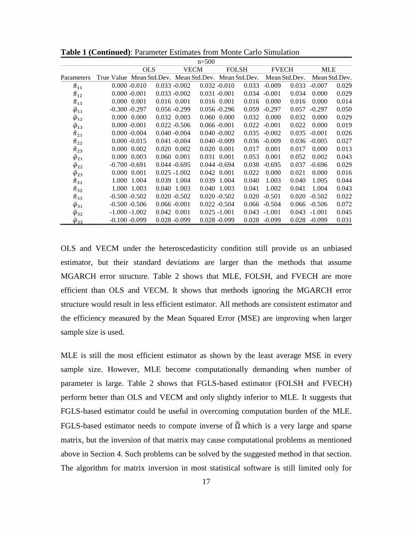
OLS and VECM under the heteroscedasticity condition still provide us an unbiased
estimator, but their standard deviations are larger than the methods that assume
MGARCH error structure. Table 2 shows that MLE, FOLSH, and FVECH are more
efficient than OLS and VECM. It shows that methods ignoring the MGARCH error
structure would result in less efficient estimator. All methods are consistent estimator and
the efficiency measured by the Mean Squared Error (MSE) are improving when larger
sample size is used.
MLE is still the most efficient estimator as shown by the least average MSE in every
sample size. However, MLE become computationally demanding when number of
parameter is large. Table 2 shows that FGLS-based estimator (FOLSH and FVECH)
perform better than OLS and VECM and only slightly inferior to MLE. It suggests that
FGLS-based estimator could be useful in overcoming computation burden of the MLE.
FGLS-based estimator needs to compute inverse of which is a very large and sparse
matrix, but the inversion of that matrix may cause computational problems as mentioned
above in Section 4. Such problems can be solved by the suggested method in that section.
The algorithm for matrix inversion in most statistical software is still limited only for
18
matrix in small dimension. We already tried to compute using standard command in
EViews and MATLAB in our simulation, while n<100 FGLS-based estimators perform
fairly good that comparable to MLE. However, when n becomes larger (i.e. n=300 and
n=500), the FGLS-based estimator become poorly inefficient since it produces extreme
values for the estimated parameters. All estimated parameters from FGLS-based
estimators presented in this paper are based on our matrix inversion procedure. The
results based on standard matrix inversion in statistical software are not presented to save
space.
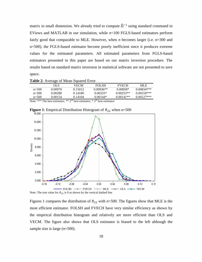
Table 2: Average of Mean Squared Error
OLS VECM FOLSH FVECH MLE
n=100 0.00970 0.15012
0.00936**
0.00958* 0.00834***
n=300 0.00280 0.14180
0.00255*
0.00253** 0.00218***
n=500 0.00154 0.14104
0.00144*
0.00141** 0.00127***
Note: *** The best estimator, ** 2nd best estimator, * 3rd best estimator
Figure 1: Empirical Distribution Histogram of when n=500
Note: The true value for is 0 as shown by the vertical dashed line
Figures 1 compares the distribution of with n=500. The figures show that MLE is the
most efficient estimator. FOLSH and FVECH have very similar efficiency as shown by
the empirical distribution histogram and relatively are more efficient than OLS and
VECM. The figure also shows that OLS estimator is biased to the left although the
sample size is large (n=500).
0.000
2.000
4.000
6.000
8.000
10.000
12.000
14.000
16.000
-0.16 -0.12 -0.08 -0.04 0.00 0.04 0.08 0.12 0.16
FOLSH FVECH MLE OLS VECM
Den
sity

19
Figure 2: Empirical Distribution Histogram of by MLE
Note: The vertical dashed line indicates the true value of the parameter
Figure 3: Empirical Distribution Histogram of by FOLSH
Note: The vertical dashed line indicates the true value of the parameter.
0.000
2.000
4.000
6.000
8.000
10.000
12.000
14.000
16.000
-0.60 -0.50 -0.40 -0.30 -0.20 -0.10 0.00 0.10 0.20 0.30
MLE, n=100 MLE, n=300 MLE, n=500
Den
sity
0.000
2.000
4.000
6.000
8.000
10.000
12.000
-0.60 -0.50 -0.40 -0.30 -0.20 -0.10 0.00 0.10 0.20 0.30
FOLSH, n=100 FOLSH, n=300 FOLSH, n=500
Den
sity
20
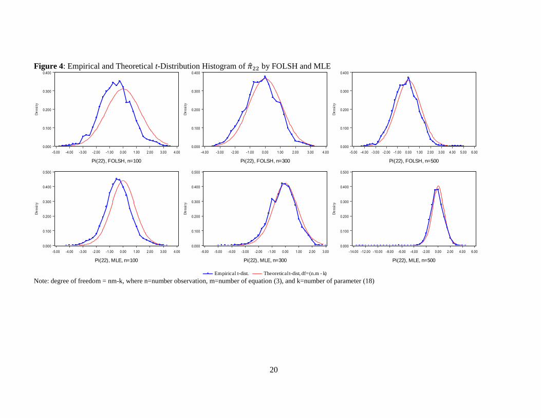
Figure 4: Empirical and Theoretical t-Distribution Histogram of by FOLSH and MLE
Note: degree of freedom = nm-k, where n=number observation, m=number of equation (3), and k=number of parameter (18)
0.000
0.100
0.200
0.300
0.400
-5.00 -4.00 -3.00 -2.00 -1.00 0.00 1.00 2.00 3.00 4.00
De
nsi
ty
Pi(22), FOLSH, n=100
0.000
0.100
0.200
0.300
0.400
-4.00 -3.00 -2.00 -1.00 0.00 1.00 2.00 3.00 4.00
De
nsi
ty
Pi(22), FOLSH, n=300
0.000
0.100
0.200
0.300
0.400
-5.00 -4.00 -3.00 -2.00 -1.00 0.00 1.00 2.00 3.00 4.00 5.00 6.00
De
nsi
ty
Pi(22), FOLSH, n=500
0.000
0.100
0.200
0.300
0.400
0.500
-5.00 -4.00 -3.00 -2.00 -1.00 0.00 1.00 2.00 3.00 4.00
De
nsi
ty
Pi(22), MLE, n=100
0.000
0.100
0.200
0.300
0.400
0.500
-6.00 -5.00 -4.00 -3.00 -2.00 -1.00 0.00 1.00 2.00 3.00
De
nsi
ty
Pi(22), MLE, n=300
0.000
0.100
0.200
0.300
0.400
0.500
-14.00 -12.00 -10.00 -8.00 -6.00 -4.00 -2.00 0.00 2.00 4.00 6.00
Empirical t-dist. Theoretical t-dist, df=(n.m - k)
De
nsi
ty
Pi(22), MLE, n=500
21
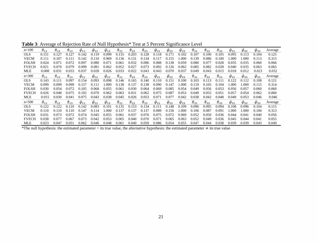
Table 3: Average of Rejection Rate of Null Hypothesis* Test at 5 Percent Significance Level n=100 Average
OLS 0.151 0.127 0.127 0.142 0.119 0.099 0.135 0.203 0.128 0.118 0.171 0.102 0.107 0.100 0.105 0.095 0.113 0.104 0.125
VECM 0.111 0.107 0.111 0.142 0.110 0.969 0.136 0.131 0.134 0.117 0.155 1.000 0.139 0.086 0.100 1.000 1.000 0.113 0.315
FOLSH 0.024 0.071 0.072 0.097 0.080 0.071 0.061 0.032 0.086 0.088 0.138 0.059 0.080 0.077 0.028 0.035 0.035 0.060 0.066
FVECH 0.021 0.070 0.079 0.099 0.081 0.062 0.052 0.027 0.073 0.092 0.126 0.062 0.085 0.082 0.028 0.040 0.035 0.063 0.065
MLE 0.008 0.031 0.033 0.037 0.028 0.026 0.033 0.022 0.043 0.043 0.070 0.037 0.049 0.043 0.015 0.018 0.012 0.023 0.032
n=300 Average
OLS 0.143 0.111 0.097 0.154 0.093 0.098 0.146 0.165 0.140 0.110 0.151 0.100 0.103 0.113 0.111 0.122 0.112 0.108 0.121
VECM 0.099 0.099 0.099 0.157 0.111 1.000 0.138 0.137 0.138 0.090 0.147 1.000 0.119 0.105 0.104 1.000 1.000 0.115 0.314
FOLSH 0.030 0.054 0.072 0.105 0.068 0.055 0.061 0.030 0.064 0.069 0.085 0.054 0.049 0.056 0.053 0.056 0.057 0.060 0.060
FVECH 0.026 0.048 0.075 0.102 0.070 0.062 0.063 0.031 0.062 0.075 0.087 0.053 0.049 0.055 0.051 0.057 0.054 0.062 0.060
MLE 0.015 0.030 0.041 0.075 0.043 0.038 0.045 0.026 0.053 0.071 0.077 0.042 0.038 0.042 0.048 0.049 0.053 0.046 0.046
n=500 Average
OLS 0.122 0.122 0.110 0.142 0.083 0.101 0.135 0.153 0.134 0.111 0.148 0.109 0.096 0.095 0.094 0.108 0.096 0.104 0.115
VECM 0.110 0.110 0.110 0.147 0.114 1.000 0.137 0.137 0.137 0.089 0.156 1.000 0.106 0.087 0.091 1.000 1.000 0.106 0.313
FOLSH 0.031 0.073 0.072 0.074 0.045 0.055 0.061 0.037 0.076 0.075 0.072 0.069 0.052 0.050 0.036 0.044 0.041 0.040 0.056
FVECH 0.038 0.077 0.067 0.073 0.042 0.053 0.065 0.040 0.070 0.071 0.065 0.063 0.052 0.049 0.036 0.045 0.044 0.041 0.055
MLE 0.023 0.047 0.051 0.062 0.046 0.048 0.061 0.040 0.059 0.086 0.054 0.055 0.047 0.044 0.038 0.039 0.039 0.043 0.049
*The null hypothesis: the estimated parameter = its true value, the alternative hypothesis: the estimated parameter its true value

22
Figure 2 and 3 show example of empirical distribution of the estimated parameter
by MLE and FOLSH respectively, for n=100, 300, and 500. Those figures suggest
that both ML estimator and FOLSH are consistent estimators as the estimated
parameter more converge to the true value when the sample size is larger. Both MLE
and FOLSH tend to be unbiased when sample size is large.
Figure 4 shows example of empirical t-statistic distribution for . From the figures,
both FOLSH and MLE tend to conform to student-t distribution when larger sample
size is used. The empirical distribution for estimated by FVECH is very similar to
that by FOLSH. Table 3 shows that rejection rate of null hypothesis that each
parameter is equal to its true value is also close to the significance level (0.05) for
parameter estimated by FOLSH, FVECH, and MLE. From the table it is also apparent
that estimators that do not consider multivariate GARCH error structure (OLS and
VECM) has higher rejection rate compares to those of estimators that consider the
error structure (FOLSH, FVECH, and MLE). These findings show us that neglecting
the presence of multivariate GARCH error structure will increase the rejection rate or
the type I error.
5. EMPIRICAL APPLICATION
Weekly data from July 1997 until July 2011 of US S&P500, Japan Nikkei225 and
Malaysia KLSE composite index are collected as a dataset for our model (n=732).
The indexes are stated in logarithmic and are measured in US Dollar. Since they are
in log index, their first order differences can be regarded as stock market return of the
respective markets.
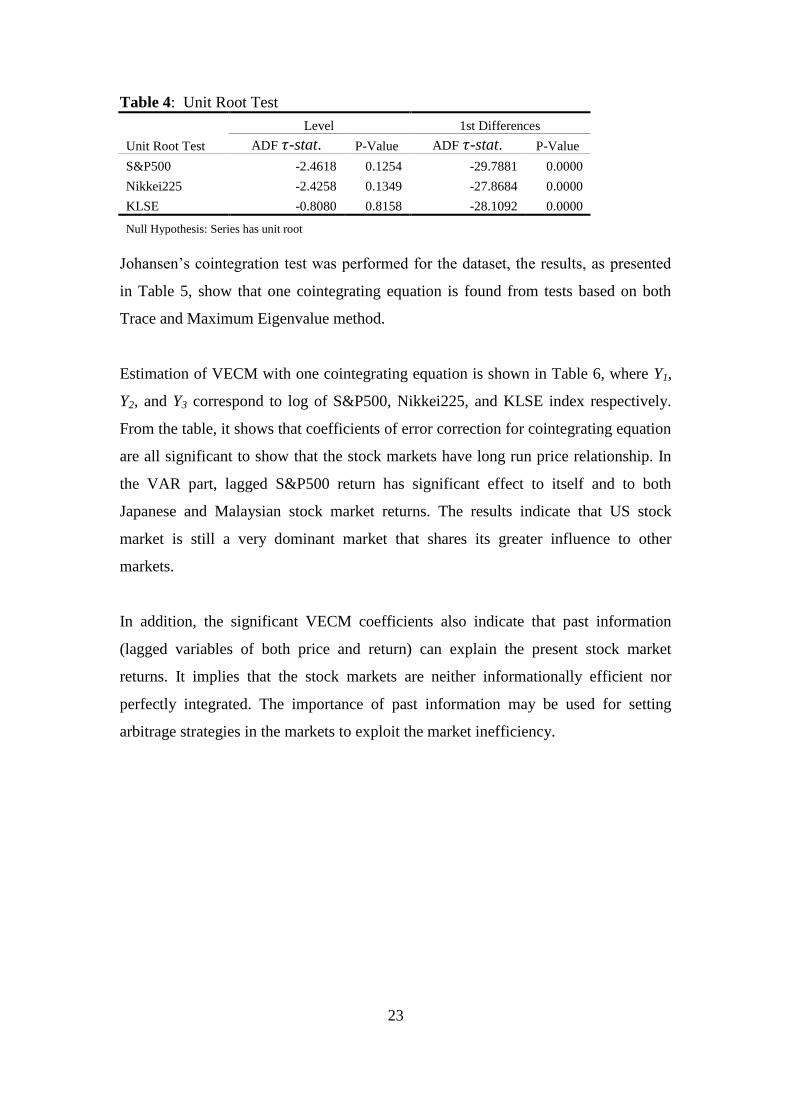
Unit root test indicates that the three time series are non-stationary at level, but they
are stationary at their first difference. The Augmented Dickey Fuller (ADF) statistic
( -stat.) for data in level indicates the null hypothesis that the series has unit root
cannot be rejected at 10 percent significance level or less. Meanwhile, the -stat. for
the respective series in the first order difference significantly rejects the null
hypothesis of unit root at one percent significance level.
23
Table 4: Unit Root Test
Level 1st Differences
Unit Root Test ADF -stat. P-Value ADF -stat. P-Value
S&P500 -2.4618 0.1254 -29.7881 0.0000
Nikkei225 -2.4258 0.1349 -27.8684 0.0000
KLSE -0.8080 0.8158 -28.1092 0.0000
Null Hypothesis: Series has unit root
Johansen‟s cointegration test was performed for the dataset, the results, as presented
in Table 5, show that one cointegrating equation is found from tests based on both
Trace and Maximum Eigenvalue method.
Estimation of VECM with one cointegrating equation is shown in Table 6, where Y1,
Y2, and Y3 correspond to log of S&P500, Nikkei225, and KLSE index respectively.
From the table, it shows that coefficients of error correction for cointegrating equation
are all significant to show that the stock markets have long run price relationship. In
the VAR part, lagged S&P500 return has significant effect to itself and to both
Japanese and Malaysian stock market returns. The results indicate that US stock
market is still a very dominant market that shares its greater influence to other
markets.
In addition, the significant VECM coefficients also indicate that past information
(lagged variables of both price and return) can explain the present stock market
returns. It implies that the stock markets are neither informationally efficient nor
perfectly integrated. The importance of past information may be used for setting
arbitrage strategies in the markets to exploit the market inefficiency.

24
Table 5: Johansen Cointegration Test
Unrestricted Cointegration Rank Test (Trace)
Hypothesized Trace 0.05
No. of CE(s) Eigenvalue Statistic Critical Value Prob.**
None * 0.0436 38.0006 29.7971 0.0046
At most 1 0.0058 5.4141 15.4947 0.7634
At most 2 0.0016 1.1569 3.8415 0.2821
Unrestricted Cointegration Rank Test (Maximum Eigenvalue)
Hypothesized Max-Eigen 0.05
No. of CE(s) Eigenvalue Statistic Critical Value Prob.**
None * 0.0436 32.5865 21.1316 0.0008
At most 1 0.0058 4.2572 14.2646 0.8313
At most 2 0.0016 1.1569 3.8415 0.2821
Trace and Max-eigenvalue test indicates 1 cointegrating eqn(s) at the 0.05 level * denotes rejection of the hypothesis at the 0.05 level
**MacKinnon-Haug-Michelis (1999) p-values
Table 6: Vector Error Correction Model (VECM) Coint.Eq. Coef.
Y1t-1 1.000
Y2t-1 -0.682
(0.090)
Y3t-1 -0.024
(0.054)
C -3.700
E.C. Eq. ∆Y1t ∆Y2t ∆Y3t
Coint.Eq. -0.024 0.027 0.040
(0.009) (0.012) (0.015)
∆Y1t-1 -0.095 0.214 0.174
(0.041) (0.053) (0.069)
∆Y2t-1 -0.007 -0.076 0.032
(0.032) (0.042) (0.055)
∆Y3t-1 0.012 -0.047 -0.076
(0.024) (0.031) (0.040)
C 0.000 -0.001 0.000
(0.001) (0.001) (0.002)
Standard Error in Parenthesis
25
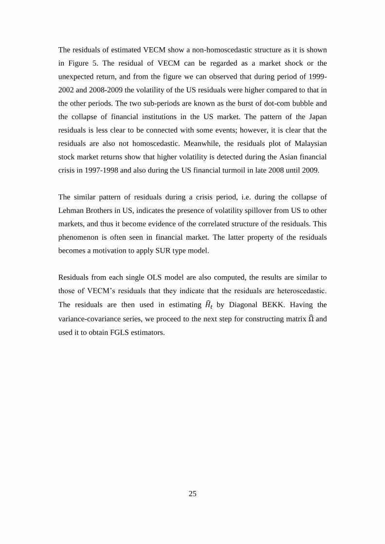
The residuals of estimated VECM show a non-homoscedastic structure as it is shown
in Figure 5. The residual of VECM can be regarded as a market shock or the
unexpected return, and from the figure we can observed that during period of 1999-
2002 and 2008-2009 the volatility of the US residuals were higher compared to that in
the other periods. The two sub-periods are known as the burst of dot-com bubble and
the collapse of financial institutions in the US market. The pattern of the Japan
residuals is less clear to be connected with some events; however, it is clear that the
residuals are also not homoscedastic. Meanwhile, the residuals plot of Malaysian
stock market returns show that higher volatility is detected during the Asian financial
crisis in 1997-1998 and also during the US financial turmoil in late 2008 until 2009.
The similar pattern of residuals during a crisis period, i.e. during the collapse of
Lehman Brothers in US, indicates the presence of volatility spillover from US to other
markets, and thus it become evidence of the correlated structure of the residuals. This
phenomenon is often seen in financial market. The latter property of the residuals
becomes a motivation to apply SUR type model.
Residuals from each single OLS model are also computed, the results are similar to
those of VECM‟s residuals that they indicate that the residuals are heteroscedastic.
The residuals are then used in estimating by Diagonal BEKK. Having the
variance-covariance series, we proceed to the next step for constructing matrix and
used it to obtain FGLS estimators.

26
Figure 5: Residuals of VECM
-0.200
-0.150
-0.100
-0.050
0.000
0.050
0.100
0.150
1997 1998 1999 2000 2001 2002 2003 2004 2005 2006 2007 2008 2009 2010 2011
Residuals of D(Ln(S&P500))
-0.200
-0.100
0.000
0.100
0.200
1997 1998 1999 2000 2001 2002 2003 2004 2005 2006 2007 2008 2009 2010 2011
Residuals of D(Ln(Nikkei225))
-0.400
-0.200
0.000
0.200
0.400
1997 1998 1999 2000 2001 2002 2003 2004 2005 2006 2007 2008 2009 2010 2011
Residuals of D(Ln(KLSE))

27
Figure 6: Estimated Conditional Variance-Covariance
(a) Conditional Variance
(b) Conditional Covariance
The FGLS estimators, the restated VECM (without GARCH), OLS, and MLE
estimated parameters are shown in Table 7. As shown in the table, although the sign
and value of the estimated parameters are very similar among the various estimation
methods, but the probability of significance are sometime different. Based on the data
properties shown in Figure 5 and 6, the GARCH error structure does exists. And
based on the simulation results, estimation methods that take into account the
GARCH structure are more efficient than those that ignore the structure. Therefore, in
the empirical example, the use of such methods (OLS and VECM) might produce
0.000
0.005
0.010
0.015
0.020
0.025
0.030
97 98 99 00 01 02 03 04 05 06 07 08 09 10 11
Var(US) Var(JP) Var(MY)
-0.001
0.000
0.001
0.002
0.003
0.004
0.005
97 98 99 00 01 02 03 04 05 06 07 08 09 10 11
Covar(US-JP) Covar(US-MY) Covar(JP-MY)

28
wrong conclusion regarding the significance of the estimated parameters. For
example, estimated by OLS (and VECM) is significantly different from zero, but
it is not significant when it is estimated by FOLSH, FVECH, and MLE. It means that
when we estimate the parameter using method that neglecting the MGARCH error
structure we would conclude that lagged of Nikkei225 Index (Japanese stock prices)
affects Malaysia KLSE returns (Malaysian stock returns), while we should not.
Table 6: Estimated Parameters of OLS, VECM, FOLSH, FVECH, and MLE
Estimated
Parameter
OLS VECM FOLSH FVECH MLE
Coef. S.E. Coef. S.E. Coef. S.E. Coef. S.E. Coef. S.E.
0.139 0.047
** 0.089 #
0.138 0.045
** 0.195 0.045
** 0.139
0.038
**
-0.028 0.009 **
-0.024 #
-0.029 0.010 **
-0.040 0.010 **
-0.024
0.007 **
0.014 0.007 *
0.016 #
0.014 0.004 **
0.019 0.004 **
0.008
0.004
-0.001 0.003
0.001 #
0.000 0.000 **
0.000 0.000 **
-0.001
0.002
-0.093 0.041 *
-0.095 0.041 *
-0.091 0.159
-0.090 0.061
-0.106
0.040 **
-0.006 0.032
-0.007 0.032
0.007 0.010
0.008 0.005
-0.004
0.024
0.013 0.024
0.012 0.024
0.038 0.028
0.038 0.017 *
0.035
0.015 *
-0.023 0.061
-0.102 #
-0.017 0.025
0.028 0.016
* -0.006
0.048
0.020 0.012
0.027 #
0.015 0.016
0.005 0.003 *
0.019
0.009 *
-0.024 0.009 **
-0.019 #
-0.020 0.031
-0.015 0.009 *
-0.023
0.006 **
-0.001 0.003
-0.001 #
0.001 0.002
0.001 0.000 *
-0.003
0.003
0.218 0.053 **
0.214 0.053 **
0.259 0.086 **
0.261 0.066 **
0.200
0.042 **
-0.075 0.042
-0.076 0.042
-0.094 0.045 *
-0.095 0.031 **
-0.050
0.038
-0.046 0.031
-0.047 0.031
-0.056 0.037
-0.057 0.023 **
-0.026
0.022
-0.129 0.079
-0.147 #
-0.109 0.272
-0.052 0.035
-0.017
0.050
0.040 0.016 *
0.040 #
0.026 0.041
0.011 0.007 *
0.007
0.011
-0.026 0.011 *
-0.027 #
-0.014 0.029
-0.004 0.003
-0.003
0.008
-0.005 0.004
-0.001 #
-0.001 0.001
-0.001 0.001
-0.003
0.004
0.173 0.069 *
0.174 0.069 *
0.246 0.119 *
0.251 0.082 **
0.223
0.036 **
0.031 0.055
0.032 0.055
0.006 0.003 *
0.002 0.001 **
0.011
0.030
-0.073 0.040
-0.076 0.040
-0.067 0.041
-0.061 0.023 **
-0.026
0.037
** significant at 0.01
* significant at 0.05
The Standard error marked by # indicates that the coefficient is computed from loading vector and
adjustment vector in the error correction equations, the respective standard error for these parameters
are shown in Table 5.
6. CONCLUDING REMARKS
The standard Vector Error correction model (VECM), which is based on normality
assumption of error term, is often applied to analyze the real financial time series.
However, as shown in the section 5 it is often seen that residuals of this model seem

29
to follow GARCH errors process. From this experience we extend the standard
VECM to include GARCH error process. We call such model as VEC-GARCH
model. Although the maximum likelihood (ML) estimator is known as the most
efficient estimator under the normality assumption, ML estimation is computationally
demanding when a model to be estimated is not small. To overcome these
disadvantages and to reduce computational burden of ML estimator we consider the
generalized least square estimator (GLS) instead of ML estimator. GLS is relatively
free from the distributional assumptions.
In this paper we mainly concerns with the GLS representation, the algorithm of it, and
the properties of it, we have examined the performance of GLS and MLE in VEC-
GARCH model by Monte Carlo simulation and the applicability of it by real data
analysis of the financial time series. The Monte Carlo simulation naturally has shown
that MLE is still better than the FGLS. However FGLS-based estimators that also
consider GARCH error structure are also more efficient than estimators that neglect
the error structure. The performance of MLE and FGLS-based estimator in our
simulation are only slightly different, yet both are better estimators compare to the
OLS and VECM. Thus, the suggested FGLS-based estimator may overcome the
disadvantages of MLE, especially in reducing the computational burden.
Our suggested method for the large matrix inversion successfully overcomes the
computational problem such as memory size, computer time, and innacurate
numerical results. The estimated parameters from the FGLS-based estimator
performed in the simulation is as good as the MLE.
There, however, remain several problems in estimating VECM with GARCH errors
for the future research as follows: (1) to use realized volatility (RV) instead of
multivariate GARCH model, (2) to compare the GLS and MLE under non-normality
by Monte Carlo simulation, (3) to carry out theoretical comparisons of asymptotic
properties of the GLS and MLE, under normality and non-normality, (4) to examine
the performance of VEC model with GARCH errors when it is applied to empirical
analysis of financial time series. We have a plan to attack these problems in future.

30
REFERENCES
Bauwens, L., S. Laurent and J. V. K. Rombouts (2006). Multivaritae GARCH
Models: a survey, Journal of applied Econometrics, 21: 79-109.
Bollerslev, T., R.F.Engle and J.M.Wooldridge (1988). A Capital asset pricing model
with time varying covariances, Journal of Political Economy 96, 116-131.
Engle, R. F. and K. F. Kroner (1995). Multivariate Simultaneous Generalized ARCH.
Econometric theory, 11, 122-150.
Johansen, S. (1995). Likelihood-based Inference in Cointegrated Vector
autoregressive Models, Oxford: Oxford University Press.
Johnston, J. and J. DiNardo (2007). Econometric Methods, McGraw-Hill Co, Inc.
Silvennoinenn, A. and T. Ter svirta (2009). Multivariate GARCH models, Handbook
of Financial Time Series, ed. by T. G. Andersen, R. A. Davis, J. P. Kreiss and
T. Mikosch, New Yor: Springer.
Zellner, A. (1962). An Efficient Method of Estimating Seemingly Unrelated
Regressions and Test of Aggregation Bias, Journal of the American Statistical
Association, 57, 500-509.

31
PART II
APPLICATION OF SUR-GARCH METHOD
IN INTERNATIONAL CAPM TEST
1. MODELS
The proposed test model is aimed to examine the relationship between expected
returns of national stock market indexes and the world market portfolio returns. The
national stock market indexes are weighted average of the constituent stocks prices
based on either market capitalization (e.g. S&P500 Index) or liquidity (e.g. Nikkei
225). The riskless asset is proxied by government securities; 3-month T-Bill.
In previous international CAPM literatures, MSCI world index or other Exchange
Traded Fund (ETF) that consists of national market indexes were used as proxy of the
world market portfolio. It should be noted that such index weighs the composing asset
based on market capitalization or liquidity where the weight is always nonnegative. It
means that the world market portfolio consists of assets in long position. Meanwhile
CAPM assumes that unrestricted short selling of those assets is allowed. One may
argue that we can short sell the index instead of short selling its composing assets.
However, the strategy of short selling the world market index does not ensure us that
the portfolio is efficient and at tangent of capital market line. To overcome these
problems, world market portfolio is constructed following Merton (1972) procedure
and Tobin‟s separation theory (Tobin, 1958) to guarantee that the portfolio is not only
mean-variance efficient, but also located at a point which is at tangent of the capital
market line.
1.1. Expected return and Conditional Variance-Covariance Matrix of Each Asset
Considering that the stock markets has long-run equilibrium with the other markets
and disturbance errors of the estimation model are correlated and heteroscedastic,
vector error correction model with GARCH (VEC-GARCH Model) is applied to
estimate the expected returns of each national market index and their conditional
32
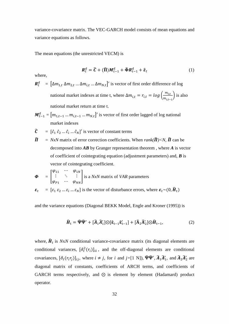
variance-covariance matrix. The VEC-GARCH model consists of mean equations and
variance equations as follows.
The mean equations (the unrestricted VECM) is
( )
(1)
where,
= [ ] is vector of first order difference of log
national market indexes at time t, where (
) is also
national market return at time t.
= [ ] is vector of first order lagged of log national
market indexes
= is vector of constant terms
= NxN matrix of error correction coefficients. When rank( )<N, can be
decomposed into AB by Granger representation theorem , where A is vector
of coefficient of cointegrating equation (adjustment parameters) and, B is
vector of cointegrating coefficient.
= [
] is a NxN matrix of VAR parameters
= is the vector of disturbance errors, where ( )
and the variance equations (Diagonal BEKK Model, Engle and Kroner (1995)) is
, (2)
where, is NxN conditional variance-covariance matrix (its diagonal elements are
conditional variances, ( ) , and the off-diagonal elements are conditional
covariances, ( ) , where , for i and j=[1 N]), , , and
are
diagonal matrix of constants, coefficients of ARCH terms, and coefficients of
GARCH terms respectively, and is element by element (Hadamard) product
operator.

33
The parameters in the mean equations and the variance equations theoretically can be
estimated by maximum likelihood estimator (MLE). However, when the system is
large as in our case, MLE often produces inaccurate results because too many
parameters need to be estimated such that the optimization of the log likelihood
function failed. To overcome this problem, the mean equation (VECM) parameters
were estimated as those in Seemingly Unrelated Regression (SUR) system using
modified feasible generalized least square (mFGLS) estimator that taking into account
the GARCH error structure. This estimation strategy was also used in testing the
CAPM and shall be explained later.
For estimating conditional variance of realized return, the mean equation in equation
(1) was replaced by and the conditional variance-covariance matrix was
estimated by Diagonal BEKK. Henceforth, accent “ ” and “ ” are used for
indicating variable based on the realized return and the estimated expected return
respectively.
1.2. World Market Portfolio Formation
World market portfolio was constructed by assuming that unrestricted short selling
and borrowing at riskless rate in domestic or national market are allowed. The
assumptions were made to follow the underlying assumptions in CAPM.
The proportion of each asset in an efficient portfolio was obtained by minimizing
objective function of portfolio variance with respect to following constraints: [1] a set
of target portfolio expected return and, [2] the sum of proportion of each asset
(including riskless asset) is equal to one. When short selling is prohibited, constraint
[2] is modified by adding restriction on proportion of each risky asset to vary between
0 to 1, yet in this paper the proportion is unrestricted to indicate that the short selling
can be done without any restriction.
Suppose that country i is our focus of analysis and call it home country. Portfolio
consists of riskless asset available at domestic market i and N international risky
portfolios (
). The rate of return of is the weighted average of rate

34
of return of its composing assets. Our objective is to construct world market portfolio
denoted by that consists of risky portfolios only (proxied by market indexes). Let
us define ( ) , and e as riskless rate of return, vector of
proportion of risky assets in portfolio and vector of ones respectively. Constraint
[2] implies that ( ) is the proportion of riskless asset in portfolio . Applying
constraint [2] to the expected return of risk-free asset and risky assets definition, the
expected return of may be stated as:
( ) (3)
Having conditional variance-covariance matrix from (2), variance of portfolio at
time t is computed by,
( )
. (4)
The optimal weight of the N risky assets and risk-free asset was obtained by solving
following optimization problem:
{
( ) }. (5)
The first-order condition of (5) leads to following solution:
( ). (6)
Taking from (6) and apply the
restriction, we may obtain :
( )
(7)
where
and .
From (6), the expected return of risky portfolio M is
and the variance of
portfolio P will be equal to the variance of portfolio M defined as ( )
( )
. Define (
) as nx1 vector of covariance of the tangency
portfolio with each of the risky asset. Then using (6) and (7), we have
( )
( ) (8)

35
Pre-multiply (8) by we have
( ) restated as
( )
( )
(
) ( ) (9)
Rearranging (8) and substituting in for m from (9) we have the CAPM:
( )
(
) (
)
( )
( ). (10)
The LHS of (10) is the expected excess return from each asset, while on the RHS,
( )
( )
is vector of time varying betas of each risky asset, and ( ) is the
expected market risk premium that prevails for all risky assets. Note that because we
are assuming that short selling is unrestricted, is always nonnegative, and the
portfolio M is always in the efficient frontier of portfolio P (the risk-free and risky
assets portfolio). However, elements of , the estimated expected return of each
asset could be positive or negative. When the expected return of an asset is negative,
it will be more likely to be short sold. Thus, ( ) is not always positive. As a result
we may find that an asset‟s beta and the beta risk premium is negative.1
1.3. Testing Conditional CAPM
The capital asset pricing model in equation (10) will serve as our test model. In
addition, because we consider international assets, we must put additional risk factor
other than the world market risk (represented by the betas) that indicates the required
adjustment for the excess return. In this paper we include exchange rate returns in the
model. We can consider the international CAPM being tested in this paper is
involving Exchange Traded Funds (ETFs) that track directly the respective stock
market indexes. Therefore, like the CAPM test for assets traded in one market, we can
ignore the transaction cost of acquiring the cross-border assets. The test model is
defined in a system equation as follows:
(11)
1 See Pennacchi (2008) pp. 37-60 for more detailed derivation of the market portfolio.
36
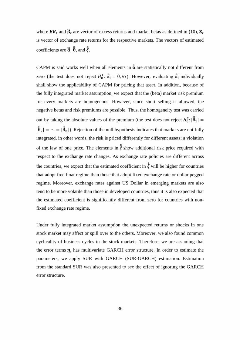
where and are vector of excess returns and market betas as defined in (10),
is vector of exchange rate returns for the respective markets. The vectors of estimated
coefficients are , , and .
CAPM is said works well when all elements in are statistically not different from
zero (the test does not reject : ). However, evaluating individually
shall show the applicability of CAPM for pricing that asset. In addition, because of
the fully integrated market assumption, we expect that the (beta) market risk premium
for every markets are homogenous. However, since short selling is allowed, the
negative betas and risk premiums are possible. Thus, the homogeneity test was carried
out by taking the absolute values of the premium (the test does not reject | |
| | | |). Rejection of the null hypothesis indicates that markets are not fully
integrated, in other words, the risk is priced differently for different assets; a violation
of the law of one price. The elements in show additional risk price required with
respect to the exchange rate changes. As exchange rate policies are different across
the countries, we expect that the estimated coefficient in will be higher for countries
that adopt free float regime than those that adopt fixed exchange rate or dollar pegged
regime. Moreover, exchange rates against US Dollar in emerging markets are also
tend to be more volatile than those in developed countries, thus it is also expected that
the estimated coefficient is significantly different from zero for countries with non-
fixed exchange rate regime.
Under fully integrated market assumption the unexpected returns or shocks in one
stock market may affect or spill over to the others. Moreover, we also found common
cyclicality of business cycles in the stock markets. Therefore, we are assuming that
the error terms has multivariate GARCH error structure. In order to estimate the
parameters, we apply SUR with GARCH (SUR-GARCH) estimation. Estimation
from the standard SUR was also presented to see the effect of ignoring the GARCH
error structure.

37
2. ESTIMATION STRATEGY
Equation (1) and (11) can be restated as SUR model. For simplicity, we will use
system equation (11) as a sample to explain the estimation strategy.
Let us define as T-vector of excess return of asset-i, matrix is
vector of independent variables, where its respective elements are T-vector of ones, T-
vector of time varying beta for asset-i, and T-vector of exchange rate changes for
market-i, and , , is vector of coefficients for equation-i. Then, equation-i
in the system equation (11) can be restated as follows:
(12)
where is T-vector of the disturbance errors for the equation. In stacked model, the
system equation (11) can be restated as follows:
[
] [
] [
] [
],
In general, the corresponding matrices define the following system,
. (13)
VECM in system equation (1) also can be stated similar to the above system equation
by redefining the and accordingly. To reduce the number of parameters needs to
be estimated in the VEC-GARCH, we first estimate the VECM (without GARCH),
create series of cointegrating equation (we assume that there is only one cointegrating
equation), and use it as new variable in a VAR system. Thus, the for system
equation (1) defined as , where CE is T-vector of cointegrating
series that applied for every i.
2.1. Feasible Generalized Least Square (FGLS) SUR Estimation
FGLS or also known as Zellner‟s estimator (Zelner, 1962), assumes that
| (strict exogeneity of Xi), and |
(homoscedasticity). As stock markets are assumed to be fully integrated, the

38
disturbances might be correlated across equations. Therefore,
[ | ] for and 0 for . The is covariance
between disturbances i and j; it is ijth element of variance-covariance matrix . Let us
also define The generalized least square estimator under the covariance
structures assumption is
( )
( )
. (14)
Because is generally unknown, it is estimated by
where is
vector of residuals in equation i. By doing so, the estimated variance-covariance
matrix can be computed. The FGLS estimator requires inversion of matrix , so that
the matrix must have a non-zero discriminant.
The standard errors of the parameters were estimated by taking the square root of
elements in sampling variances:
[ | ] ( ) (15)
where,
( ) ( )
.
The join hypotheses of and
, were tested by Wald coefficient test with J degree
of freedom, where J is N and N-1 respectively. The restriction is defined by ,
where R is (JxK) matrix of restriction with K is number of the parameters in , and q
is J-vector of the true values. The Wald statistic is distributed and computed by
( ) ( ) ( ). (16)
2.2. Modified Feasible Generalized Least Square (mFGLS) SUR-GARCH
Estimation
Considering that system equation (1) and (11) are estimated in fully integrated
markets and there were shocks and crises during the observation periods that spilled
over among the samples, the multivariate GARCH error structure should be
considered. To do so, following is steps to include the error structure for estimating
the parameters in the models:

39
[1] Estimate the mean equations by first ignoring the GARCH error structure and
obtain the residuals.
[2] Use the residuals to estimates conditional variance-covariance matrix by
using Diagonal BEKK model. At every observation t, we have with
elements of .
[3] Use the variance-covariance matrix from step 2 to construct . Note that in
(14) is defined as where the diagonal elements are the vector of
variances of each equation (which is a constant variance) and the off-diagonal
elements are all zeros (there is no covariance across the equations). The
modified at this step is considering the heteroscedasticity and covariance
across the equations. To illustrate it in a simple example, for N= 3, is:
[
]
where, is a NxN diagonal matrix where its main diagonal elements are
elements of N-vector of and zeros on the off-diagonal elements, and
, i.e.,
[
]

40
Thus we have,
k
k
where follow multivariate MGARCH(1,1) process.
After obtaining an estimate , we have the modified FGLS,
(17)
Note that inverting a large and sparse matrix often causes computational
problems such as memory size, computer time, and inaccurate numerical
results. To avoid those problems we propose the following algorithm: After
estimating MGARCH process we construct a relatively small matrix and
its inverse at each time t such that,
[
] [
]
where and are estimated variance covariance of MGARCH.
Replacing with
in we have easily obtain without inverting a
large matrix
Having the modified and the hypotheses can be tested using the Wald Test as
described previously. The performance of the modified FGLS estimator has been
examined by carrying out Monte Carlo simulation. The modified FGLS estimator is
41
still an unbiased estimator and it is more efficient and consistent than the standard
FGLS estimator when multivariate GARCH error structure does exist (Maekawa and
Setiawan, 2012).
3. DATA
Stock market index from 12 economies were collected with its respective currency.
The indexes represent 6 developed stock markets: United States S&P500 (US),
Germany DAX (GE), Hong Kong Hang Seng (HK), Japan Nikkei225 (JP), Singapore
Strait Times (SI) and FTSE100 (UK), and 6 emerging markets: Argentina MerVal
(AR), Brazil BOVESPA (BR), China SSEC (CH), Indonesia IDX composite (ID),
Malaysia KLSE composite (MA), and Mexico IPC (ME). The market indexes are
exchange rate adjusted, with US Dollar as the home currency.
The dataset starts from July 1997 to July 2012 and in weekly basis for avoiding non-
synchronous trading time effect. Data were collected from Yahoo Finance service
through its website. Because weekly data is used, and it is assumed that portfolios
rebalancing are done weekly, the returns are not including dividends. Most of the
stock market indexes are value-weighted indexes and the remaining are equally
weighted index and top performers‟ index. However, the indexes used in this paper
are assumed sufficient in representing the market portfolio in the respective markets
because the indexes used to be regarded as the market references. As the US is
regarded as home country, US 3-month T-Bills is used as the risk-free rate.
4. FINDINGS
4.1. Data Properties
Based on Augmented Dickey-Fuller (ADF) Tests and Common Unit Root Tests
performed for data in level (log market index) and its first difference (return), the
results indicate that all series in level are non-stationary (except for Indonesia and
Malaysia when intercept and trend are included), but all series in its first difference
are stationary.
Granger causality test for returns of the US Dollar adjusted market indexes were
performed, and the results are shown in Table 1. It indicates that US stock market
Granger-caused the other markets (except for China, Malaysia and Mexico). The
42
result implies that US stock market is still very dominant and has greater influence to
other markets in the world.
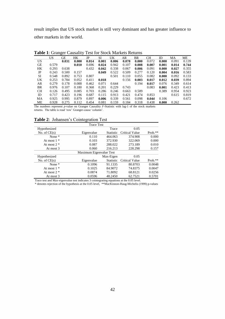
Table 1: Granger Causality Test for Stock Markets Returns
US GE HK JP SI UK AR BR CH ID MA ME
US
0.031 0.000 0.014 0.001 0.006 0.078 0.000 0.072 0.000 0.091 0.139 GE 0.579
0.010 0.696 0.024 0.942 0.107 0.008 0.007 0.001 0.014 0.744
HK 0.293 0.638
0.432 0.042 0.338 0.067 0.006 0.091 0.000 0.027 0.355 JP 0.243 0.500 0.157
0.049 0.522 0.509 0.277 0.120 0.004 0.016 0.583
SI 0.548 0.892 0.753 0.807
0.501 0.110 0.055 0.082 0.000 0.092 0.133 UK 0.253 0.784 0.052 0.411 0.018
0.156 0.003 0.017 0.012 0.039 0.894
AR 0.279 0.178 0.088 0.462 0.071 0.644
0.194 0.017 0.076 0.349 0.614 BR 0.976 0.107 0.180 0.368 0.201 0.229 0.743
0.083 0.001 0.423 0.413
CH 0.126 0.495 0.085 0.703 0.286 0.246 0.663 0.589
0.389 0.954 0.923 ID 0.717 0.423 0.196 0.687 0.115 0.913 0.421 0.474 0.853
0.615 0.819
MA 0.925 0.995 0.879 0.897 0.006 0.339 0.561 0.098 0.044 0.106
0.672 ME 0.928 0.275 0.112 0.454 0.081 0.159 0.184 0.318 0.438 0.000 0.262
The numbers represent p-value on Granger Causality F-Statistic with lag-1 of the stock markets
returns. The table is read „row‟ Granger-cause „column‟.
Table 2: Johansen‟s Cointegration Test Trace Test
Hypothesized
Trace 0.05
No. of CE(s) Eigenvalue Statistic Critical Value Prob.**
None * 0.110 464.063 374.908 0.000
At most 1 * 0.103 372.930 322.069 0.000
At most 2 * 0.087 288.022 273.189 0.010
At most 3 0.060 216.213 228.298 0.157
Maximum Eigenvalue Test
Hypothesized
Max-Eigen 0.05
No. of CE(s) Eigenvalue Statistic Critical Value Prob.**
None * 0.1096 91.1335 80.8703 0.0048
At most 1 * 0.1025 84.9072 74.8375 0.0047
At most 2 * 0.0874 71.8092 68.8121 0.0256
At most 3 0.0596 48.2450 62.7521 0.5701
Trace test and Max-eigenvalue test indicates 3 cointegrating equations at the 0.05 level.
* denotes rejection of the hypothesis at the 0.05 level, **MacKinnon-Haug-Michelis (1999) p-values

43
The cointegration test in Table 2 shows that there are three cointegrating equations. It
shows that there is long-term equilibrium relationship among the market indices.
However, for simplicity and reducing computational burden in VECM estimation,
only one cointegrating equation was applied. The cointegrating equation in the
VECM is shown in Table 3. Using the cointegration equation, VECM and VEC-
GARCH Model parameters are shown in Table 4 and 5.
Table 3: Cointegrating Equation in Vector Error Correction Model (VECM)
log(US) log(GE) log(HK) log(JP) log(SI) log(UK) log(AR) log(BR) log(CH) log(ID) log(MA) log(ME) Const.
Coeff. 1.000 0.094 0.526 -0.371 0.021 -0.528 -0.138 -0.008 -0.022 0.364 -0.996 -0.023 2.027
S.E.
-0.170 -0.182 -0.127 -0.234 -0.167 -0.061 -0.091 -0.055 -0.071 -0.140 -0.082 -1.002
t-stat.
0.554 2.884 -2.916 0.090 -3.153 -2.282 -0.083 -0.397 5.117 -7.131 -0.282 2.024
Number in bold face indicates the coefficient is significant at 5% level.
Table 4: Vector Error Correction Model (VECM)
Coint.Eq. -0.027 -0.022 0.011 0.027 0.021 -0.017 -0.002 -0.019 -0.025 0.043 0.095 -0.011
S.E. -0.009 -0.014 -0.013 -0.012 -0.013 -0.010 -0.019 -0.021 -0.012 -0.022 -0.014 -0.015
-0.034 0.159 0.218 0.203 0.185 0.171 0.071 0.289 -0.023 0.107 -0.049 0.182
S.E. -0.062 -0.092 -0.088 -0.078 -0.088 -0.069 -0.128 -0.138 -0.083 -0.148 -0.093 -0.103
0.006 -0.178 0.043 -0.064 -0.004 -0.066 0.046 0.020 0.080 0.090 0.091 -0.002
S.E. -0.045 -0.067 -0.065 -0.057 -0.064 -0.050 -0.094 -0.101 -0.060 -0.108 -0.068 -0.076
-0.004 0.021 -0.050 0.012 0.041 0.028 0.088 0.137 0.018 0.080 0.017 0.036
S.E. -0.042 -0.063 -0.060 -0.053 -0.060 -0.047 -0.087 -0.094 -0.056 -0.101 -0.063 -0.070
-0.033 0.018 0.021 -0.064 0.029 0.002 -0.037 -0.052 0.005 0.022 0.064 -0.072
S.E. -0.036 -0.053 -0.051 -0.045 -0.051 -0.040 -0.074 -0.080 -0.048 -0.086 -0.054 -0.060
0.007 -0.005 -0.002 -0.015 -0.128 -0.004 0.066 -0.040 -0.007 0.199 0.012 0.105
S.E. -0.042 -0.062 -0.060 -0.053 -0.059 -0.046 -0.086 -0.093 -0.056 -0.100 -0.063 -0.070
-0.049 -0.062 -0.057 -0.007 0.025 -0.177 -0.039 0.038 0.021 -0.193 0.034 -0.110
S.E. -0.062 -0.092 -0.088 -0.078 -0.088 -0.069 -0.128 -0.138 -0.082 -0.147 -0.093 -0.103
-0.027 0.024 0.033 0.011 0.028 -0.009 -0.001 0.027 0.051 -0.027 0.017 0.022
S.E. -0.023 -0.034 -0.032 -0.029 -0.032 -0.025 -0.047 -0.050 -0.030 -0.054 -0.034 -0.038
0.012 0.034 -0.004 0.009 -0.017 0.012 -0.037 -0.130 0.022 0.042 -0.020 -0.050
S.E. -0.024 -0.036 -0.034 -0.030 -0.034 -0.027 -0.050 -0.054 -0.032 -0.057 -0.036 -0.040
-0.044 -0.035 -0.059 -0.009 -0.050 -0.043 -0.045 -0.006 0.002 -0.105 0.006 -0.012
S.E. -0.028 -0.042 -0.040 -0.035 -0.040 -0.031 -0.058 -0.062 -0.037 -0.067 -0.042 -0.046
0.009 -0.020 -0.033 -0.017 0.019 0.001 -0.052 0.007 -0.020 -0.047 -0.060 -0.013
S.E. -0.018 -0.027 -0.026 -0.023 -0.026 -0.020 -0.037 -0.040 -0.024 -0.043 -0.027 -0.030
0.003 0.003 0.007 0.012 0.105 0.019 0.005 0.043 0.057 -0.010 0.025 -0.017
S.E. -0.029 -0.043 -0.041 -0.037 -0.041 -0.032 -0.060 -0.065 -0.039 -0.069 -0.044 -0.048
0.023 -0.019 -0.025 -0.029 -0.021 0.008 0.033 -0.084 -0.085 0.058 -0.016 -0.027
S.E. -0.036 -0.053 -0.051 -0.045 -0.051 -0.040 -0.074 -0.079 -0.048 -0.085 -0.054 -0.059
Number in bold face indicates the coefficient is significant at 5% level.

44
Table 5: VEC-GARCH Model By Modified FGLS Estimator
Coint.Eq. -0.021 -0.025 0.019 0.030 0.025 -0.014 0.001 -0.041 -0.017 0.035 0.095 -0.011
S.E. 0.006 0.008 0.010 0.008 0.009 0.007 0.010 0.016 0.011 0.017 0.012 0.011
-0.106 0.044 0.149 0.131 0.165 0.083 0.005 -0.016 -0.056 0.217 -0.012 0.000
S.E. 0.050 0.071 0.066 0.068 0.061 0.053 0.100 0.111 0.078 0.100 0.060 0.082
0.032 -0.117 0.094 -0.043 0.034 -0.059 0.076 0.033 0.080 0.055 0.094 0.044
S.E. 0.037 0.056 0.048 0.050 0.045 0.040 0.074 0.081 0.057 0.070 0.044 0.058
0.018 0.076 -0.051 0.034 0.017 0.102 0.109 0.279 0.018 0.037 0.016 0.059
S.E. 0.031 0.044 0.046 0.043 0.041 0.033 0.060 0.074 0.051 0.073 0.045 0.053
-0.029 0.025 -0.031 -0.060 0.023 0.007 -0.010 -0.078 -0.013 0.018 0.004 -0.089
S.E. 0.028 0.040 0.038 0.042 0.035 0.029 0.058 0.065 0.044 0.060 0.036 0.047
-0.004 -0.042 -0.027 -0.009 -0.107 -0.049 0.009 -0.085 -0.019 0.064 0.016 0.039
S.E. 0.032 0.046 0.049 0.046 0.046 0.034 0.066 0.079 0.051 0.078 0.048 0.057
0.028 0.061 -0.018 0.051 -0.038 -0.048 0.017 0.199 0.057 -0.172 -0.054 0.042
S.E. 0.050 0.073 0.064 0.068 0.059 0.055 0.101 0.112 0.078 0.095 0.059 0.080
-0.015 0.021 0.029 0.016 0.048 -0.003 0.035 0.032 0.052 -0.027 0.025 0.048
S.E. 0.018 0.028 0.023 0.027 0.022 0.019 0.044 0.041 0.028 0.034 0.021 0.029
-0.002 0.012 -0.006 0.001 -0.013 -0.011 0.009 -0.096 0.005 0.065 0.010 -0.020
S.E. 0.019 0.028 0.025 0.027 0.023 0.020 0.040 0.045 0.030 0.039 0.024 0.031
-0.068 -0.071 -0.074 -0.069 -0.073 -0.083 -0.145 -0.129 0.005 -0.118 0.002 -0.097
S.E. 0.020 0.029 0.027 0.029 0.025 0.022 0.041 0.046 0.036 0.043 0.026 0.034
0.014 -0.008 -0.043 -0.009 0.027 0.002 0.003 0.043 -0.031 0.030 -0.063 0.013
S.E. 0.014 0.019 0.023 0.021 0.021 0.015 0.030 0.037 0.022 0.041 0.024 0.026
0.028 0.051 0.085 0.015 0.132 0.056 0.044 0.071 0.069 0.069 0.089 0.028
S.E. 0.023 0.031 0.035 0.030 0.032 0.023 0.044 0.056 0.036 0.058 0.040 0.040
0.031 -0.024 -0.002 -0.025 0.014 0.014 -0.035 -0.099 -0.056 -0.002 0.010 -0.048
S.E. 0.028 0.040 0.038 0.040 0.035 0.029 0.058 0.066 0.045 0.061 0.035 0.049
Number in bold face indicates the coefficient is significant at 5% level.
4.2. Expected Return of Risky Asset
The estimated parameters and their standard errors in the VECM and VEC-GARCH
model are different. Because MGARCH error structure is assumed, the estimated
expected returns are based on the VEC-GARCH model.
The statistics of the estimated expected return and realized return are presented in
Table 6. In general, emerging stock markets such as Brazil, China, and Mexico had
higher expected return, yet they were also more volatile than those in the developed
markets. Several economic crises and recessions took place during the observation
period, such that the averages of expected returns in most countries were negative.
The long period of recession in Japan was causing both its realized and expected
returns are negative. In emerging markets, only stock market in Argentina that
consistently has negative realized and expected return.

45
Table 6: Annualized Weekly Statistics Realized Return US GE HK JP SI UK AR BR CH ID MA ME
Mean 0.024 0.034 0.015 -0.030 0.033 0.004 -0.029 0.044 0.056 0.020 0.014 0.096
Std.Dev. 0.178 0.265 0.255 0.225 0.255 0.199 0.367 0.397 0.238 0.430 0.275 0.295
Expected Return* US GE HK JP SI UK AR BR CH ID MA ME
Mean 0.008 -0.001 -0.005 -0.014 -0.010 0.002 -0.006 0.000 0.002 -0.005 -0.031 -0.001
Std.Dev. 0.026 0.033 0.048 0.035 0.061 0.031 0.057 0.081 0.037 0.081 0.076 0.039
*The estimated expected return was estimated by VEC-GARCH using modified FGLS estimator
4.3. Conditional Variance of Risky Asset
Conditional variances for each market expected return were estimated using Diagonal
BEKK model of Engle and Kroner (1995) as specified in equation (2) and the results
are shown in Figure 1 and 2 for the developed and emerging markets respectively.
The figures show that the conditional variances were increasing during period of
crises, yet the magnitudes varied across the samples. For example, non-Asian
developed and emerging stock markets were less affected by the Asian financial crisis
in 1997-1998. However, the US financial crisis in 2008-2009 seems spilled over to
other markets and the Asian markets were becoming more volatile in that period.
Emerging markets apparently show higher volatility than that for the developed
markets. The different magnitudes of volatility indicate that there is opportunity to
obtain lower diversifiable risk by investing in those markets; this could be the driving
factor of stronger price comovements and stock market integration.

46
Figure 1: Conditional Variance of Estimated Expected Return in Developed
Markets
Note: Shaded area is the US recession period (based on NBER Business Cycle Dating Committee
report, last update was on September 20, 2010).
Figure 2: Conditional Variance of Estimated Expected Return in Emerging Markets
Note: The scale was trimmed to conform to the Figure 1. Shaded area is the US recession period
(based on NBER Business Cycle Dating Committee report, last update was on September 20, 2010).
0.00000
0.00004
0.00008
0.00012
0.00016
0.00020
97 98 99 00 01 02 03 04 05 06 07 08 09 10 11 12
US GE HK
JP SI UKDeveloped Stock Market:
0.00000
0.00004
0.00008
0.00012
0.00016
0.00020
97 98 99 00 01 02 03 04 05 06 07 08 09 10 11 12
AR BR CH
ID MA MEEmerging Stock Market:
47
4.4. Test of International CAPM
The ex-ante and ex-post test for the CAPM were carried out under both SUR (without
GARCH) and SUR-GARCH. The results are shown in Table 7 and 8 respectively. In
ex-ante test (Table 7), the null hypotheses and
are all rejected, they indicate
that CAPM does not work well for the international assets and the market risk
premiums are heterogeneous across the markets. However, individual test of the
hypothesis that (t-test) show that CAPM can be applied for pricing of all
market indexes (except for the Malaysian market), even under the SUR-GARCH test,
all alphas are not statistically different from zero. It is susceptible that the rejection of
were caused by large differences in the standard errors
2. This is an indication that
the market risk premium adjustments across the markets were so vary during the
observation period. The results suggest that removing some markets from the sample
might alter the verdict that the CAPM does not fit well for international asset pricing.
The homogeneity test of the market risk premiums are also rejected in both tests. It
suggests that the stock markets were not fully integrated yet. Market risk is priced
higher in Asian stock markets such as in Singapore, Indonesia, and Malaysia, than
that in other markets. Meanwhile, in the US and the Japan, the market risk premium is
lower than that in the other markets.
Note that all market risk premiums are nonnegative. This is the expected result. It
indicates that the constructed world market portfolio is always in the efficient frontier
and is at the tangency of capital market line.
2 The differences in the standard errors cannot be seen in the tables because the numbers were rounded to only three decimals.

48
Table 7: Ex-Ante International Dynamic Beta CAPM Test
SUR SUR-GARCH
Coef. S.E. t-Stat. Prob. Coef. S.E. t-Stat. Prob.
0.000 0.000 1.885 0.059 0.000 0.000 0.279 0.781
0.021 0.000 51.835 0.000 0.021 0.000 74.689 0.000
0.000 0.000 1.144 0.253 0.000 0.000 -1.152 0.252
0.022 0.000 65.176 0.000 0.022 0.000 95.359 0.000
-0.002 0.003 -0.596 0.552 -0.001 0.002 -0.564 0.574
0.000 0.000 0.180 0.857 0.000 0.000 1.747 0.084
0.022 0.000 70.061 0.000 0.022 0.000 104.130 0.000
0.066 0.056 1.175 0.240 0.063 0.031 2.032 0.045
0.000 0.000 -2.233 0.026 0.000 0.000 0.165 0.869
0.022 0.000 71.136 0.000 0.021 0.000 105.469 0.000
0.002 0.003 0.829 0.407 0.002 0.002 0.951 0.344
0.000 0.000 -0.349 0.727 0.000 0.000 0.293 0.770
0.024 0.000 67.676 0.000 0.023 0.000 101.945 0.000
0.018 0.010 1.765 0.078 0.012 0.006 2.037 0.044
0.000 0.000 1.751 0.080 0.000 0.000 0.043 0.966
0.022 0.000 71.038 0.000 0.022 0.000 103.266 0.000
0.001 0.003 0.465 0.642 0.002 0.002 0.822 0.413
0.000 0.000 -0.122 0.903 0.000 0.000 0.053 0.958
0.023 0.000 81.410 0.000 0.022 0.000 121.855 0.000
0.000 0.003 -0.098 0.922 0.000 0.002 -0.143 0.886
0.000 0.000 0.820 0.412 0.000 0.000 -1.226 0.223
0.023 0.000 62.376 0.000 0.022 0.000 92.981 0.000
0.000 0.005 -0.007 0.994 0.001 0.003 0.253 0.801
0.000 0.000 -0.298 0.766 0.000 0.000 -1.898 0.061
0.022 0.000 75.680 0.000 0.021 0.000 102.483 0.000
-0.040 0.023 -1.710 0.087 -0.011 0.015 -0.749 0.455
0.000 0.000 -0.721 0.471 0.000 0.000 0.426 0.671
0.024 0.000 67.258 0.000 0.023 0.000 103.701 0.000
0.003 0.002 1.471 0.141 0.003 0.001 1.943 0.055
-0.001 0.000 -2.937 0.003 0.000 0.000 0.765 0.446
0.024 0.000 53.605 0.000 0.023 0.000 91.641 0.000
0.008 0.008 0.929 0.353 0.004 0.005 0.774 0.441
0.000 0.000 -0.348 0.728 0.000 0.000 -1.380 0.171
0.022 0.000 69.672 0.000 0.022 0.000 99.530 0.000
0.000 0.003 -0.126 0.900 0.000 0.002 -0.177 0.860
Coefficients Wald Test
Null Hypothesis d.f. Chi-sq Prob.
d.f. Chi-sq Prob.
12 30.843 0.002
12 26.463 0.009
| | | | | | 11 69.525 0.000
11 174.795 0.000
Number in bold face indicates the coefficient is significant at 5% level.
The effect of changes in currency exchange rates seemed to be absorbed by the
market risk factor. Under the SUR-GARCH test, the additional required rate of return
to compensate the exchange rate risk is only applied for assets from Hong Kong and
Singapore stock market. This result indicates that the market risk (beta) is still the
only relevant risk factor in the International CAPM (provided that un-integrated stock
markets were removed from the sample such that could not be rejected).

49
Table 8: Ex-Post International Dynamic Beta CAPM Test
SUR SUR-GARCH
Coef. S.E. t-Stat. Prob. Coef. S.E. t-Stat. Prob.
0.000 0.001 0.199 0.842 0.000 0.000 0.670 0.504
-0.019 0.003 -6.893 0.000 -0.015 0.002 -8.040 0.000
0.000 0.001 0.219 0.827 0.000 0.001 0.472 0.638
-0.017 0.003 -6.124 0.000 -0.011 0.002 -5.722 0.000
0.644 0.051 12.604 0.000 0.652 0.036 18.327 0.000
0.000 0.001 -0.346 0.729 0.000 0.001 -0.222 0.825
-0.006 0.003 -1.792 0.073 -0.002 0.002 -0.793 0.430
1.300 0.830 1.566 0.117 1.782 0.485 3.672 0.000
-0.001 0.001 -1.316 0.188 -0.002 0.001 -2.260 0.026
-0.011 0.003 -3.260 0.001 -0.007 0.002 -3.027 0.003
0.658 0.062 10.635 0.000 0.623 0.045 13.819 0.000
-0.001 0.001 -0.737 0.461 0.000 0.001 -0.007 0.994
-0.003 0.003 -0.977 0.329 0.000 0.002 0.023 0.981
1.227 0.102 11.996 0.000 1.112 0.061 18.143 0.000
0.000 0.001 0.236 0.813 0.000 0.000 0.150 0.881
-0.018 0.002 -7.196 0.000 -0.012 0.002 -7.459 0.000
0.653 0.040 16.178 0.000 0.661 0.027 24.050 0.000
-0.002 0.002 -0.928 0.353 -0.002 0.001 -1.898 0.061
0.008 0.004 2.189 0.029 0.008 0.003 3.051 0.003
0.345 0.072 4.759 0.000 0.462 0.077 6.027 0.000
-0.001 0.002 -0.408 0.683 0.001 0.001 0.591 0.556
-0.005 0.003 -1.717 0.086 -0.005 0.002 -2.877 0.005
1.037 0.054 19.222 0.000 1.050 0.035 30.399 0.000
0.000 0.001 -0.350 0.726 -0.001 0.001 -0.647 0.519
0.002 0.004 0.568 0.570 0.005 0.003 1.558 0.122
0.853 0.736 1.159 0.247 1.389 0.524 2.652 0.009
0.000 0.002 -0.078 0.938 0.003 0.001 2.919 0.004
-0.001 0.003 -0.424 0.671 0.001 0.002 0.476 0.635
0.978 0.035 28.243 0.000 1.064 0.032 33.572 0.000
0.000 0.001 -0.276 0.783 0.001 0.001 1.404 0.163
-0.004 0.004 -1.014 0.310 0.002 0.002 0.674 0.502
1.093 0.081 13.481 0.000 1.090 0.061 17.976 0.000
0.002 0.001 1.391 0.164 0.003 0.001 3.718 0.000
-0.007 0.003 -2.307 0.021 -0.007 0.002 -3.845 0.000
1.128 0.071 15.891 0.000 1.067 0.042 25.520 0.000
Coefficients Wald Test
Null Hypothesis d.f. Chi-sq Prob.
d.f. Chi-sq Prob.
12 9.442 0.665
12 45.876 0.000
| | | | | | 11 36.816 0.000
11 148.947 0.000
Number in bold face indicates the coefficient is significant at 5% level.
The ex-post test presented in Table 8 examined whether CAPM was applied in the
market for pricing the international assets. The test was using realized or actual
returns. From the table, CAPM fits well in pricing the assets when multivariate
GARCH error structure was ignored (the test under SUR). Testing the alphas
individually shall support the finding. However, from the data properties of the
sample, the multivariate GARCH error structure does exist. Ignoring the error
structure proved that the latter conclusion was inaccurate; when GARCH error
structure was considered, the CAPM does not fit well! This result is inline with
previous findings, for example in Lewellen and Nagel (2006) and Wu and Chiou
50
(2007). The latter paper used Kalman filter method in testing the CAPM. Thus, this
paper shows the applicability of SUR-GARCH model using the modified FGLS
estimator that is simpler than other method such as the Kalman filter.
As the previous analysis in the ex-ante test, removing some stock market indexes
might make CAPM works. Under the SUR-GARCH test, CAPM only failed to work
for pricing the Japanese and the Indonesian stock market returns. This research shows
that constructing world market portfolio from the twelve indexes leads to inapplicable
CAPM. Finding the stock market indexes that make CAPM works is subject to future
research.
The realized market risk premiums are also heterogeneous. Some of the market risk
premiums are negative. They indicate that those indexes returns have negative
covariance with the world market portfolio. This is as a result of allowing the short
selling. Moreover, this result also suggests that the stock markets were not fully
integrated yet. The price of the market risk for the assets varies. In addition, exchange
rate risk is also priced differently for the market indexes. It indicates that beta risk is
not the only risk factor considered by investors. Multi factors CAPM may be applied
in the markets.
5. CONCLUSIONS
Conditional International CAPM was tested under assumptions of unrestricted short
selling and borrowing at riskless rate such that the constructed world market portfolio
is a mean-variance efficient portfolio at the tangency of the capital market line.
Previous researches that attempt to test the CAPM for international assets were using
readily available index that was subject to the critique that the market portfolio was
not mean-variance efficient. By constructing the world market portfolio that meets
with the assumptions, we could estimates not only the expected return and conditional
variance of that portfolio, but also the conditional covariance between the world
market portfolio and its composing portfolios (national stock market indices), such
that time varying betas for each international asset can be estimated. Thus, all
assumptions used in building the CAPM were all met so that the test of the model can
be emphasized on the estimated parameters of the model.
51
The test of the international asset-pricing model was carried out by assuming that the
markets were fully integrated so that covariance among the disturbance terms is not
zero. Furthermore, because crises, recession, and other kind of market shocks
happened during the observation period in 1997:7 until 2012:7, heteroscedasticity of
the errors is expected, and the sample data properties said so. To consider the
covariance and the heteroscedasticity, the time varying beta CAPM was tested under
SUR-GARCH model. In ex-ante test CAPM is rejected, but individual analysis of the
assets showed that CAPM may be applied for all of the assets. It indicates that the risk
premium adjustments were done during the period of analysis, and the levels of
adjustments varied across the assets. The market risk is also priced differently for
each assets, it indicates that the markets were not fully integrated yet. However,
exchange rate risk is not significantly affecting the expected excess return. The latter
shows that theoretically CAPM is correct, that the only risk factor worth to consider is
the market risk (beta). However, in the real world, the ex-post tests show that CAPM
had failed in pricing the international assets and it suggests that other risk factors
might exist.
The findings are subject to the stock market index selection for constructing the world
market portfolio. In addition, CAPM might also work under sub-sample periods, for
example under non-recession period. Finding the structural break point under SUR-
GARCH also a challenge in the econometric side. These issues should be addressed in
the future research.
REFERENCES
Bekaert, G., and Harvey, C. R. (1995). Time-Varying World Market Integration. The
Journal of Finance, 50:2, pp. 403–444.
Black, F. (1972). Capital market equilibrium with restricted borrowing, Journal of
Business, Vol. 45, pp. 444–55.
Bollerslev, T., Engle, R. F. and Wooldridge, J. M. (1988). Capital asset pricing model
with time-varying covariances, Journal of Political Economy, 96, 116–31.
Breitung, Jörg (2000). The Local Power of Some Unit Root Tests for Panel Data, in
B. Baltagi (ed.), Advances in Econometrics, Vol. 15: Nonstationary Panels, Panel
Cointegration, and Dynamic Panels, Amsterdam: JAI Press, p. 161–178.
Chan, Louis K.C., Yasushi Hamao and Josef Lakonishok. (1991). Fundamentals and
Stock Returns in Japan, Journal of Finance, 46:5, pp. 1739–789.

52
Chen, Z., and Knez, P. J. (1995). Measurement of Market Integration and Arbitrage,
The Review of Financial Studies, 8:2, pp.287–325.
Das, S. and R. Uppal, (2004). Systemic Risk and International Portfolio Choice,
Journal of Finance, 59:6, pp. 2809-2834.
deBondt, Werner F. M. and Richard H. Thaler, (1987). Further Evidence on Investor
Overreaction and Stock Market Seasonality, Journal of Finance. 42:3, pp. 557–
81.
Engel, C., and Rodrigues, A. P., (1989). Tests of international CAPM with time-
varying covariances. Journal of Applied Econometrics, Vol. 4, 119–138.
Engle, Robert F. and K. F. Kroner, (1995). Multivariate Simultaneous Generalized
ARCH, Econometric Theory, 11, pp. 122-150.
Fama, E. F., and French, K. R. (1992). The cross-section of expected stock returns,
Journal of Finance, pp. 427–465.
Fama, E. F., and French, K. R., (2004). The Capital Asset Pricing Model: Theory and
Evidence, Journal of Economic Perspectives, 18, pp. 25–46.
Fama, E. F., and MacBeth, J. D., (1973). Risk, return, and equilibrium: Empirical
tests, The Journal of Political Economy, 81(3), pp. 607–636.
Fama, E.F. and French, K.R., (1998). Value Versus Growth: The International
Evidence. Journal of Finance, 53:6, pp. 1975–999.
Fernandez, V. P. (2005). The international CAPM and a wavelet-based decomposition
of value at risk, Studies in Nonlinear Dynamics & Econometrics, 9:4, pp.1–35.
Fischer Black and Robert Litterman, (1992). Global Portfolio Optimization, Financial
Analysts Journal, 48:5, pp. 28-43
French, K. R., and Poterba, J. M. (1991). Investor Diversification and International
Equity Markets, The American Economic Review, 81(2), pp. 222–226.
Gibbons, M. R., Ross, S. A., and Shanken, J. (1989). A test of the efficiency of a
given portfolio. Econometrica, Journal of the Econometric Society, pp. 1121–
1152.
Greene, W. H. (2008). Econometric Analysis, Prentice Hall, Boston.
Hadri, Kaddour (2000). Testing for Stationarity in Heterogeneous Panel Data,
Econometric Journal, 3, pp. 148–161.
Haugen, R. A., and Baker, N. L. (1991). The efficient market inefficiency of
capitalization-weighted stock portfolios. The Journal of Portfolio Management,
(Spring), 35–40.
Kothari, S. P., Jay Shanken and Richard G. Sloan. (1995). Another Look at the Cross-
Section of Expected Stock Returns, Journal of Finance, 50:1, pp. 185–224.
Kumar, P., Sorescu, S. M., Boehme, R. D., and Danielsen, B. R. (2008). Estimation
Risk, Information, and the Conditional CAPM: Theory and Evidence, Review of
Financial Studies, 21:3, pp. 1037–1075.
Levin, A., C. F. Lin, and C. Chu (2002). Unit Root Tests in Panel Data: Asymptotic
and Finite-Sample Properties, Journal of Econometrics, 108, 1–24.
Levy, H. (2010). The CAPM is Alive and Well: A Review and Synthesis. European
Financial Management, 16(1), pp. 43–71.
Levy, M. (2008). CAPM risk-return tests and the length of the sampling period,
Working Paper, Hebrew University.
Lewellen, J., and Nagel, S. (2006). The Conditional CAPM does not explain asset-
pricing anomalies, Journal of Financial Economics, 82, 289-314.
Lintner, J., (1965). The Valuation of Risk Assets and the Selection of Risky
Investments m Stock Portfolios and Capital Budgets, Review of Economics and

53
Statistics, pp. 13-37.
MacKinnon, J.G., Haug, A.A., and Michelis, L., (1999), Numerical Distribution
Functions of Likelihood Ratio Tests for Cointegration, Journal of Applied
Econometrics, 14, pp. 563-577.
Maekawa, K., and Setiawan, K., (2012), Estimation of Vector Error Correction Model
with GARCH Errors, Proceeding on SMU-ESSEC Symposium on Empirical
Finance & Financial Econometrics, 8-9 June 2012, Singapore.
Merton, R.C., (1972). An analytic derivation of the efficient portfolio frontier,
Journal of Financial and Quantitative Analysis, 7, pp. 1851–72.
Pennachi, G. (2008). Theory of Asset Pricing, Pearson, Boston.
Sharpe, W., (1964). Capital Asset Prices: A Theory of Market Equilibrium under
Conditions of Risk. Journal of Finance, pp. 425-442.
Tobin, J. (1958). Liquidity Preference as Behavior Towards Risk, The Review of
Economic Studies, 67, pp. 65–86.
Tsuji, C. (2009). Can We Resurrect the CAPM in Japan? Evaluating Conditional
Asset Pricing Models by Incorporating Time-varying Price of Risk. Research in
Applied Economics, 1:1.
Wu, P. S., & Chiou, J. S. (2007). Multivariate test of Sharpe-Lintner CAPM with
Time-Varying Beta. Applied Financial Economics Letters, 3(5), 335–341.
Wu, H. (2008). International Asset Pricing Models: A Forecasting Evaluation,
International Research Journal of Finance and Economics, 15, pp. 175–184.
Zellner, A. (1962). An efficient method of estimating seemingly unrelated regressions
and tests for regression bias, Journal of the American Statistical Association, 57,
348–6.