ESTIMATORS OF THE INTERGENERATIONAL ELASTICITY OF EXPECTED INCOME

Pablo A. Mitnik (pmitnik@stanford.edu)

December, 2017

The Stanford Center on Poverty and Inequality is a program of the Institute for Research in the Social Sciences at Stanford University.

Abstract

The intergenerational income elasticity (IGE) conventionally estimated in the mobility literature

has been widely misinterpreted as pertaining to the conditional expectation of children’s income,

when in fact it pertains to its conditional geometric mean. In line with recent work, this article

focuses on the estimation of the IGE of expected income. It proposes that, in the one-sample

context, estimation of this IGE be based on the Poisson Pseudo Maximum Likelihood estimator,

or on a Generalized Method of Moments (GMM) instrumental variable estimator of the Poisson

or exponential regression model, depending on the parental information available. These

estimators can also be used together to generate a set estimate of the IGE of the expectation. In

the two-sample context, the article proposes that estimation be based on a recently advanced

two-sample GMM estimator of the exponential regression model. The article explains how to use

official Stata commands to estimate the IGE of the expectation with the first two estimators, and

how to construct confidence intervals for the partially identified IGE when their estimates are

combined to generate a set estimate. It also introduces the user-written program igets, which

implements the third estimator as well as a GMM version of the Two-Sample Two-Stage Least

Squares estimator, and thus allows to use Stata to estimate both the IGE of the expectation and

the IGE of the geometric mean when the income information for parents and children is available

in two independent samples.

1. Introduction

The intergenerational elasticity (IGE) is the workhorse measure of intergenerational

economic mobility. It has been widely estimated over the last four decades, very often with the

goal of providing a summary assessment of the level of income or earnings mobility within a

country (for reviews, see Solon 1999:1778-1788; Corak 2006; Jäntti and Jenkins 2015:Secs.

10.5.2 and 10.5.3). Beyond this elementary goal, the IGE has been used, among other purposes,

to conduct comparative analyses of economic mobility and persistence across countries, regions,

demographic groups, cohorts, and time periods (e.g., Chadwick and Solon 2002; Hertz 2005,

2007; Aaronson and Mazumder 2008; Björklund and Jäntti 2000; Mayer and Lopoo 2008;

Bloome and Western 2011); to examine the relationship between cross-sectional economic

inequality and mobility across generations (e.g., Corak 2013; Bloome 2015); and to theoretically

model and empirically study the impact of social policies and political institutions on inequality

of opportunity (e.g., Solon 2004; Bratsberg et al. 2007; Landersø and Heckman 2016).

Now, despite the IGE’s centrality in the intergenerational-mobility field, Mitnik and

Grusky (2017) have recently shown that this elasticity has been widely misinterpreted. Indeed,

the IGE has been construed as pertaining to the expectation of children’s income conditional on

their parents’ income—as apparent, for instance, in its oft-invoked interpretation as a measure of

regression to the (arithmetic) mean. However, the IGE estimated in the literature pertains to the

conditional geometric mean of the children’s income. As explained later, this not only makes all

conventional interpretations of the IGE invalid but also has very deleterious methodological

consequences.

Mitnik and Grusky (2017) have argued that both the conceptual and the methodological

problems can be solved in a straightforward manner by simply replacing the IGE of the

2

geometric mean (the de facto estimated IGE) by the IGE of the expectation (the IGE that

mobility scholars thought they were estimating) as the workhorse intergenerational elasticity.

They also called for effectuating such replacement, which requires identifying appropriate

estimators.

In line with recent work that has estimated the IGE of the expectation (Mitnik et al. 2015;

Mitnik and Grusky 2017; Mitnik 2017a; Mitnik 2017b; Mitnik 2017c), I propose that when

income information for both parents and children is included in the same sample, estimation of

that IGE be based, depending on the parental information available, on (a) the Poisson Pseudo

Maximum Likelihood (PPML) estimator, or (b) the additive-error version of the Generalized

Method of Moments (GMM) instrumental variables (IV) estimator of the Poisson or exponential

regression model (to which I will refer as the GMM-IVP estimator). As I explain later, in some

cases it may be useful to use these estimators together to generate a set estimate of—that is, to

“bracket” or provide bounds for—the IGE of the expectation. In the very common situation in

which the income information for parents and children is only available in independent samples,

I propose that estimation be based on the two-sample GMM estimator of the exponential

regression model advanced by Mitnik (2007c), to which I refer as the GMM-E-TS estimator.

In this article I show how to estimate the IGE of the expectation with the PPML and

GMM-IVP estimators using official Stata commands, and introduce the user-written program

igets, which implements the GMM-E-TS estimator and thus allows to estimate the IGE of the

expectation in the two-sample context; this new program also implements a GMM version of the

estimator typically employed to estimate the IGE of the geometric mean in that context, i.e. the

Two-Sample Two-Stage Least Squares (TSTSLS) estimator (see, e.g., Inoue and Solon 2010). I

also explain how to use Stata to construct the confidence interval for partially identified

3

parameters proposed by Imbens and Manski (2004), for the case where IGE bounds estimated

with the PPML and GMM-IVP estimators are combined to generate a set estimate of the IGE of

the expectation. The Stata implementation introduced here can be easily adapted for use in any

context in which the goal is to compute confidence intervals for partially identified parameters.

The structure of the rest of the paper is as follows. In the second section I explain why the

conventional IGE pertains to the conditional geometric mean of children’s income rather than to

its conditional expectation, as well as Mitnik and Grusky’s (2017) proposal to redefine the IGE

used as the workhorse measure of economic mobility. In the next three sections I identify the

estimators that can be employed to estimate the IGE of the expectation, lay out the reasons for

preferring the PPML, GMM-IVP and GMM-E-TS estimators, introduce the expression for a

confidence interval for a partially-identified IGE, and briefly discuss how to avoid “lifecycle

biases.” In the following three sections I show how to use official Stata commands to estimate

the IGE of the expectation in the one-sample context and to compute confidence intervals when

the IGE is partially identified, present the command igets, and explain how to use it to estimate

IGEs in the two-sample context. The last section offers brief concluding comments.

2. The IGE of what? Redefining the workhorse intergenerational elasticity

As already indicated, the conventionally estimated IGE has been widely misinterpreted.

While mobility scholars have interpreted it as the elasticity of the expectation of children’s

income or earnings conditional on parental income, that IGE pertains in fact to the conditional

geometric mean. Closely following Mitnik and Grusky’s (2017) analysis, the standard population

regression function (PRF) posited in the literature, which assumes the elasticity is constant across

levels of parental income, is:

𝐸𝐸(ln𝑌𝑌 |𝑥𝑥) = 𝛽𝛽0 + 𝛽𝛽1 ln 𝑥𝑥, [1]

4

where 𝑌𝑌 is the child’s long-run income or earnings, X is long-run parental income or father’s

earnings, 𝛽𝛽1 is the IGE as specified in the literature, and I use expressions like “Z|𝑤𝑤” as a

shorthand for "𝑍𝑍|𝑊𝑊 = 𝑤𝑤.” The parameter 𝛽𝛽1 is not, in the general case, the elasticity of the

conditional expectation of the child’s income. This would hold as a general result only if

𝐸𝐸(ln𝑌𝑌|𝑥𝑥) = ln𝐸𝐸(𝑌𝑌|𝑥𝑥). But, due to Jensen’s inequality, the latter is not the case. Instead, as

𝐸𝐸(ln𝑌𝑌 |𝑥𝑥) = ln exp𝐸𝐸(ln𝑌𝑌 |𝑥𝑥), and 𝐺𝐺𝐺𝐺(𝑌𝑌|𝑥𝑥) = exp𝐸𝐸(ln𝑌𝑌 |𝑥𝑥), Equation [1] is equivalent to

ln𝐺𝐺𝐺𝐺(𝑌𝑌|𝑥𝑥) = 𝛽𝛽0 + 𝛽𝛽1 ln 𝑥𝑥 , [2]

where GM denotes the geometric mean operator. Therefore, 𝛽𝛽1 is the elasticity of the conditional

geometric mean, i.e., the percentage differential in the geometric mean of children’s long-run

income with respect to a marginal percentage differential in parental long-run income.1

As the geometric mean is undefined whenever an income distribution includes zero in its

support, the IGE is undefined as well when this is the case. Mitnik and Grusky (2017:Section IV)

have argued that this has serious methodological consequences: It (a) makes it impossible to

determine the extent to which parental economic advantage is transmitted through the labor

market among women (as many women have zero earnings), and (b) greatly hinders research on

the role that marriage plays in generating the observed levels of intergenerational persistence in

family income (as many people remain single or have nonworking spouses, and therefore cannot

be included in analyses examining the relationship between people’s parental income and the

income contributed by their spouses). As a result, the study of gender and marriage dynamics in

intergenerational processes has been badly hampered. Equally important, Mitnik and Grusky

(2017:Section III) have shown that, as a consequence of mobility scholars’ expedient of dropping

children with zero earnings from samples (to address what is perceived as the problem of the

1 The parameter 𝛽𝛽1 is (also) the IGE of the expectation only when the error term satisfies very special conditions (Santos Silva and Tenreyro 2006; Petersen 2017; Wooldridge 2002:17).

5

logarithm of zero being undefined), estimation of earnings IGEs with short-run proxy earnings

measures is affected by substantial selection biases. This makes the current use of the IGE of

men’s individual earnings as an index of economic persistence and mobility in a country a rather

problematic practice.2

To address these problems, Mitnik and Grusky (2017) have called for redefining the

workhorse measure of economic mobility. This entails replacing the PRF of Equation [1] by a

PRF whose estimation delivers estimates of the IGE of the expectation in the general case. Under

the assumption of constant elasticity, that PRF can be written as:

ln𝐸𝐸(𝑌𝑌|𝑥𝑥) = 𝛼𝛼0 + 𝛼𝛼1 ln 𝑥𝑥 , [3]

where 𝑌𝑌 ≥ 0, 𝑋𝑋 > 0 and 𝛼𝛼1 = 𝑑𝑑 ln𝐸𝐸(𝑌𝑌|𝑥𝑥)𝑑𝑑 ln𝑥𝑥

is the percentage differential in the expectation of

children’s long-run income with respect to a marginal percentage differential in parental long-run

income. Crucially, (a) all interpretations incorrectly applied to the conventional IGE are correct

or approximately correct under this formulation (see Mitnik and Grusky 2017:Section V.A), and

(b) the IGE of the expectation is fully immune to the methodological problems affecting the IGE

of the geometric mean and, in particular, is very well suited for studying the role of marriage in

the intergenerational transmission of advantage (see Mitnik and Grusky 2017:Section V.B for

details; and Mitnik et al. 2015:64-68 for an empirical application).

3. Estimation of the IGE of the expectation in the one-sample context

Although IGEs are defined in terms of long-run income variables, they are nearly always

estimated with short-run proxy measures. As a result, estimation is affected by both left-side and

right-side measurement errors, i.e., by the fact that the children’s and the parents’ long-run

2 Importantly, the methodological problems discussed in this paragraph can’t be solved by replacing zeros by “small values” (Mitnik and Grusky, 2017:15-16).

6

incomes are measured with error. Regardless of IGE concept and regardless of the estimator

used, this makes IGE estimates susceptible to left-side and right-side “lifecycle biases,” which

occur when the short-run income measures are obtained when parents or children are too young

or too old for their incomes to represent lifetime income differences well (for lifecycle biases in

the estimation of the conventional IGE see, e.g., Black and Devereux 2011). To simplify the

discussion that follows, however, I assume in this section that lifecycle biases are not an issue,

and that the errors are classical in nature. I will consider lifecycle biases again in Section 5.

In the one-sample context, the conventional IGE—that is, the IGE of the geometric

mean—has mostly been estimated with the Ordinary Least Squares (OLS) and the Two-Stage

Least Squares (TSLS) estimators. Making the IGE of the expectation the workhorse measure of

economic persistence, as proposed by Mitnik and Grusky (2017), requires identifying estimators

that can play for the estimation of this IGE the same roles that those estimators have played for

the estimation of the conventional IGE.

3.1. Estimation with multi-year averages of parental income

OLS has been, by far, the approach most commonly used to estimate the conventional

IGE in the one-sample context. After substituting short-run income variables for the long-run

income variables in Equation [1], estimation has been carried out almost in the same way it

would be carried out with the long-run variables.3 However, due to the use of short-run income

variables, estimation is affected by right-side attenuation bias (e.g., Solon 1999; Mazumder

2005). Formal analyses (e.g., Solon 1992; Haider and Solon 2006) indicate that using as the

proxy measure a multiyear average of parents’ income—rather than a single-year measure—can

3 The only difference is that polynomials in the parents’ and the children’s ages are customarily added as controls, to account for within-generation differences in the ages at which incomes are measured. For an argument against controlling for parental age, see Mitnik et al. (2015:40-41).

7

be expected to reduce attenuation bias. Moreover, there is strong evidence that the bias may be

substantially shrunken this way, although there is disagreement on how many years of

information are necessary to eliminate the bulk of it (see Mitnik et al. 2015:7-15).

Several estimators may be used to estimate the IGE of the expectation in the same

contexts in which the OLS estimator has been used to estimate the IGE of the geometric mean.

These include the Nonlinear Least Squares estimator and PML estimators relying on various

distributions in the linear exponential family (Poisson, gamma, inverse Gaussian).4 There are

good reasons, however, to prefer the PPML estimator employed by Mitnik et al. (2015), Mitnik

and Grusky (2017), and Mitnik (2017a; 2017b). Santos Silva and Tenreyro (2006, 2011)

provided conceptual arguments and empirical evidence favoring the use of this estimator for the

estimation of constant-elasticity models. In addition, Mitnik et al. (2015:ftn. 40) reported that, in

some cases, the PPML estimator worked better than the gamma PML estimator for the

estimation of the IGE of the expectation (for the latter estimator, see Manning and Mullahy

2001).

After substituting short-run income variables for the long-run income variables in

Equation [3], the PPML estimator can be used to estimate the IGE of the expectation with any

data used in the past (or, more generally, that could be used) to estimate the conventional IGE by

OLS. Given that estimation of the IGE of the expectation with short-run proxy measures does not

require dropping children with zero earnings or income from samples, this IGE is fully immune

to the selection bias that may affect the estimation of the IGE of the geometric mean (see Mitnik

and Grusky 2017). Nevertheless, Mitnik (2017a) has shown that the use of short-run measures to

4 PML estimators are consistent regardless of the distribution of the dependent variable, provided that the mean function is correctly specified (Gourieroux, Monfort, and Trognon 1984).

8

estimate the IGE of the expectation with the PPML estimator produces an attenuation bias that is

qualitatively very similar to that affecting the IGE of the geometric mean. His formal analysis

indicates that the strategy of using a multiyear average of parents’ income can also be expected

to work in this case, while his empirical evidence, using data from the Panel Study of Income

Dynamics (PSID), shows that the attenuation bias decreases substantially as more years of

parental information are added. His results also indicate, however, that estimates of the IGE of

the expectation with parental measures based on three to five years of information (the measures

often used by mobility scholars) would be affected by substantial attenuation bias. In fact, it

appears that, with survey data, at least 13 years of information are needed to eliminate the bulk

of that bias.5

The PPML estimator has been implemented by several official Stata commands (more on

this latter). Therefore, information on methods and formulas can be found in the corresponding

sections of the Stata Manual and it’s not necessary to include it here.

3.2. Estimation with instrumental variables

Very often there are much fewer years of parental information available than what would

be needed to (nearly) eliminate attenuation bias, or even to reduce it substantially (it is not

uncommon that only one annual measure of parental income is available). Therefore, a natural

alternative is to address right-side measurement error by resorting to IV estimation. In the case of

the conventional IGE, mobility scholars have often used the TSLS estimator, instrumenting

error-ridden proxy measures of the logarithm of long-run parental income with variables like

years of parental education or father’s occupation (e.g., Solon 1992; Zimmerman 1992; Mulligan

5 This is similar to what has been reported for the conventional IGE with the same data (Mazumder 2016: Tables 1 and 2). Mitnik (2017a:29-30) suggests two reasons why fewer years might be needed with tax and other administrative data.

9

1997; Ng 2007). The main concern with this strategy has been, however, that the instruments

typically available (including parental education and occupation) are most likely positively

correlated with both the logarithm of short-run parental income and the error term in the PRF of

interest, making them endogenous. In this context, IV estimates may still be useful if the sign of

their asymptotic bias can be established. An analysis by Solon (1992: Appendix; see also Mitnik

2017b:8-10) achieved that for the conventional IGE, showing that if some plausible substantive

assumptions hold then the IV estimator of that IGE with the invalid instruments typically

available is upward inconsistent. The standard interpretation in the literature has been that this

result implies that IV estimates are useful as upper-bound estimates. Mitnik (2017:22-31)

provided empirical evidence fully consistent with this interpretation; he also showed that

instruments vary greatly with regards to the tightness of the upper bounds that they provide.

There are several IV estimators that could be used to estimate the IGE of the expectation

in any context in which the estimation of the conventional IGE has relied (or might rely) on

instrumental variables. These include the multiplicative- and additive-error versions of the GMM

IV estimator of the Poisson or exponential regression model (Mullahy 1997; Windmeijer and

Santos Silva 1997), and five two-step estimators: Two different quasi-maximum-likelihood IV

estimators of the Poisson or exponential regression model (Wooldridge 1999:Sec. 6.1; Mullahy

1997:590-591); a residual-inclusion estimator for nonlinear parametric models (Terza et al.

2008); and two different regression-calibration IV estimators of generalized linear models with

measurement error in covariates (Carroll et al. 2006:Ch. 6). The two GMM IV estimators seem

preferable to all other estimators. First, they make weaker assumptions, as they neither require

the functional-form assumptions that the other estimators need for their first estimation step, nor

the additional assumptions that the “predictor-substitution” estimators of Mullahy (1997:590-

10

591) and Carroll et al. (2006) invoke. Second, the GMM IV estimators involve standard

asymptotic inferential procedures, while the other estimators require using more complicated

closed-form asymptotic variance estimators (e.g., Murphy and Topel 1985; Hardin 2002), or

resampling methods.

Here I focus on the additive-error version of the GMM-IV estimator (to which, as

indicated earlier, I will refer as the GMM-IVP estimator), not because there are reasons to

believe that if performs better than its multiplicative-error counterpart, but for a pragmatic

reason. Mitnik (2017b) has advanced a formal analysis showing that when the GMM-IVP

estimator is used to estimate the IGE of the expectation with the instruments typically available,

the probability limit of the estimator is larger than the true parameter under substantive

assumptions analogous to those made by Solon (1992) in the case of the IGE of the geometric

mean. Therefore, as with the latter IGE, estimates of the IGE of the expectation obtained with the

GMM-IVP estimator and the instruments typically available can be expected to provide upper-

bound estimates. Mitnik (2017:22-31) offered empirical evidence strongly supporting the notion

that this is in fact the case. As with the conventional IGE, his results also indicate that

instruments vary greatly with regards to the tightness of the upper bounds that they provide. For

this reason, Mitnik suggested putting a good amount of effort into searching for “best invalid

instruments.” This may involve looking for additional instruments beyond those typically

employed by mobility researchers; using multiple instruments simultaneously, and possibly

including interactions between them; and exploring the effects of alternative functional forms

(e.g., entering an instrument in levels or in logarithms), as this has been shown to be very

consequential in some contexts (Reiss 2016).

The GMM-IVP estimator has been implemented by an official Stata command (more on

11

this latter). Thus, it isn’t necessary to include here information regarding methods and formulas,

as it is already available in the Stata Manual.

3.3. The bracketing strategy and inference under partial identification

If there are fewer years of parental information than what is needed to eliminate the bulk

of attenuation bias, the PPML estimator of the IGE of the expectation is downward inconsistent,

while the GMM-IVP estimator is upward inconsistent with the instruments typically available.

As a result, the probability limits of the PPML and GMM-IVP estimators “bracket” the true

value of the IGE of the expectation. This suggests—in direct analogy to what Solon (1992:400)

proposed for the conventional IGE and the OLS and IV estimators—that the PPML and GMM-

IVP estimators be used together to bracket or to provide bounds for the IGE of the expectation

(Mitnik 2017b). Now, although this “bracketing strategy” generates a set rather than a point

estimate, it is nevertheless possible to construct a confidence interval for the parameter of

interest. This can be achieved by considering the bracketing strategy from the perspective of the

partial-identification approach to inference (for this approach, see, e.g., Tamer 2010).

Indeed, the fact that the probability limits of the PPML and GMM-IVP estimators

provide a lower and an upper bound, respectively, for the IGE entails that the latter is only

“partially identified” (e.g., Manski 2003) by data on short-run incomes and the instruments: Even

if we could obtain an unlimited number of observations, we would not be able to learn the true

value of the IGE. As long as only short-run income information and invalid instruments are

available, we can only aim at learning what the range of values consistent with those data—the

“identified set” defined by the probability limits of the estimators—is. And, of course, we never

have an unlimited number of observations but, rather, need to estimate the bounds from a finite

sample. This means we need to take into account both the uncertainty due to partial identification

12

and the uncertainty regarding the estimated bounds.

Ideally, we would like to provide one confidence interval that (a) pertains to the partially

identified IGE rather than to the identified set, (b) reflects uncertainty due both to partial

identification and to sampling variability, and (c) converges to its nominal value uniformly

across values of the width of the identified set.6 Denoting the probability of type-I error by 𝛼𝛼,

and following Imbens and Manski (2004), a 100 (1 − 𝛼𝛼) % confidence interval meeting these

three requirements, denoted by 𝐶𝐶𝐶𝐶(𝛼𝛼), can be constructed as follows:

𝐶𝐶𝐶𝐶(𝛼𝛼) ≡ �𝛼𝛼�1𝑃𝑃𝑃𝑃𝑃𝑃𝑃𝑃 − 𝑐𝑐(𝛼𝛼) 𝑆𝑆𝐸𝐸� (𝛼𝛼�1𝑃𝑃𝑃𝑃𝑃𝑃𝑃𝑃), 𝛼𝛼�1𝐺𝐺𝑃𝑃𝑃𝑃−𝐼𝐼𝐼𝐼𝑃𝑃 + 𝑐𝑐(𝛼𝛼) 𝑆𝑆𝐸𝐸� (𝛼𝛼�1𝐺𝐺𝑃𝑃𝑃𝑃−𝐼𝐼𝐼𝐼𝑃𝑃)�,

where 𝑐𝑐(𝛼𝛼) solves

Φ(𝑐𝑐(𝛼𝛼) + 𝑅𝑅𝑊𝑊) −Φ�−𝑐𝑐(𝛼𝛼)� = 1 − 𝛼𝛼;

𝑅𝑅𝑊𝑊 = 𝛼𝛼�1𝐺𝐺𝑃𝑃𝑃𝑃−𝐼𝐼𝐼𝐼𝑃𝑃 − 𝛼𝛼�1𝑃𝑃𝑃𝑃𝑃𝑃𝑃𝑃

max �𝑆𝑆𝐸𝐸� (𝛼𝛼�1𝑃𝑃𝑃𝑃𝑃𝑃𝑃𝑃), 𝑆𝑆𝐸𝐸� (𝛼𝛼�1𝐺𝐺𝑃𝑃𝑃𝑃−𝐼𝐼𝐼𝐼𝑃𝑃)�

is an (estimate of) the relative width of the identified set; SE is the standard error operator; Φ(. )

denotes the CDF of the standard normal distribution; and the superscripts identify estimators.

Here, 𝑐𝑐(𝛼𝛼) is inversely related to 𝑅𝑅𝑊𝑊. With a 95 percent confidence interval, 𝑐𝑐(𝛼𝛼) is close to

Φ−1(0.90) ≅ 1.64 when the width of the identified set is large compared to sampling error, and

is equal to Φ−1(0.95) ≅ 1.96 under point identification.7

4. Estimation of the IGE of the expectation in the two-sample context

Relatively few countries count with samples in which the incomes of parents and their

children are both measured in some period during adulthood. For this reason, the conventional

6 Except for Mitnik (2017b), research using the bracketing strategy to estimate the conventional IGE has reported separate confidence intervals for the bounds estimated by the OLS and IV estimators, i.e., for the bounds of the identified set. 7 See Imbens and Manski (2004) and Stoye (2009) for detailed discussions of point (c) above, and for the rationale for this confidence interval. Mitnik (2017b:20-22) offers a brief summary of the intuition behind the latter.

13

IGE has very often been estimated not just with annual and other short-run proxy income

measures, but with short-run income measures drawn from two independent samples and using

the TSTSLS estimator (see Jerrim et al. 2016). As in the case of the one-sample estimates

generated with the TSLS estimator, and for the same reason (i.e., the endogeneity of the

instruments typically available), the two-sample estimates of that IGE have been interpreted as

upper-bound estimates. Making the IGE of the expectation the workhorse measure of economic

persistence requires identifying an estimator that can play for this IGE in the two-sample context

the same role played by the TSTSLS estimator of the conventional IGE in that context. Unlike in

the one sample-context, however, in which there are several possible estimators, here the only

option seems to be the two-sample GMM estimator of the exponential regression model

advanced by Mitnik (2017c). This estimator is based on a two-sample two-step estimator. I

present this estimator next. I first assume that the income variables are measured without error,

and then introduce measurement error into the analysis. This is followed by a description of the

approach for transforming the two-sample two-step estimator into a GMM estimator, and a brief

summary of what is known about the empirical performance of the estimator.

4.1. The two-sample two-step estimator with a valid instrument

In the two-sample context, the “main sample” has the children’s income information, the

“auxiliary sample” has the parents’ income information, and both samples have a common set of

variables (e.g., parents’ education or father’s occupation) that may be used as instruments or

predictors for the parents’ income information. Operationally, the two-sample two-step estimator

simply extends the approach used by the TSTSLS estimator of the linear regression model to the

estimation of the exponential regression model. Thus, when there is only one instrumented

variable, the first step estimates a linear projection of that variable on the instruments and any

14

other right-side variables included in the second step, using information from the auxiliary

sample; while the second step estimates the exponential regression model of interest using the

PPML estimator and the main sample, with the instrumented variable replaced by its predicted

values (which are computed with the parameters estimated in the first step).

I specify in this subsection the assumptions under which this two-sample two-step

estimator of the exponential regression model is consistent or approximately consistent when all

income variables are measured without error. Without any loss of generality, I assume in what

follows that 𝐸𝐸(𝑌𝑌) = 𝐸𝐸(ln𝑋𝑋) = 1. 8

Rewriting Equation [3] in additive-error form, the PRF of interest is

𝑌𝑌 = exp(𝛼𝛼0 + 𝛼𝛼1 ln𝑋𝑋) + Ψ, [4]

where 𝐸𝐸(Ψ|𝑥𝑥) = 0. Assuming for simplicity that there is only one quantitative instrument

denoted by T (e.g., years of parental education), the fist-step equation is the following population

linear projection:

ln𝑋𝑋 = 𝛾𝛾0 + 𝛾𝛾1𝑇𝑇 + Υ. [5]

Consider now the following assumptions, which apply to all t when relevant:

𝐴𝐴1. 𝐸𝐸(𝑅𝑅|𝑡𝑡) = 0

𝐴𝐴2.∀𝑐𝑐 > 0,𝐸𝐸(exp(𝑐𝑐𝑅𝑅)|𝑡𝑡) = 𝐸𝐸(exp(𝑐𝑐𝑅𝑅))

𝐴𝐴2′.𝑉𝑉𝑉𝑉𝑉𝑉(𝑅𝑅|t) = Var(𝑅𝑅)

𝐴𝐴3. 𝛾𝛾1 ≠ 0

𝐴𝐴4. 𝐸𝐸(Ψ|𝑡𝑡) = 𝐸𝐸(Ψ).

8 This involves no loss of generality because it can always be achieved by simply changing the monetary units used to measure income.

15

Assumptions A1 and A3 entail that the expectation of the logarithm of parental income

conditional on the value of T is a linear function of that value, while assumptions A3 and A4

entail that T is a valid instrument. Assumption A2 is similar to the standard assumption made for

the estimation of Poisson models with unobserved heterogeneity (see, e.g., Winkelman 2008).

Assumption A2’, which posits that the error in the first-step equations is homoscedastic, provides

an alternative to A2. Although A2’ is not strictly weaker than A2 (neither assumption entails the

other), the fact that the dependent variable in the first-step equation is the logarithm of an income

variable may make A2’ more attractive than A2.

I start by showing that under assumptions A1, A2, A3 and A4 the two-sample estimator

of 𝛼𝛼1 is consistent. Substituting Equation [5] into Equation [4], and using A1 and A3, yields:

𝑌𝑌 = exp(𝛼𝛼0 + 𝛼𝛼1𝐸𝐸(ln𝑋𝑋 |𝑇𝑇) + 𝛼𝛼1𝑅𝑅) + Ψ

𝐸𝐸(𝑌𝑌|𝑡𝑡) = exp�𝛼𝛼0 + 𝛼𝛼1𝐸𝐸(ln𝑋𝑋 |𝑡𝑡)� 𝐸𝐸(exp(𝛼𝛼1 𝑅𝑅)|𝑡𝑡) + 𝐸𝐸(Ψ|𝑡𝑡). [6]

Using now A2, Equation [6] reduces to:

𝐸𝐸(𝑌𝑌|𝑡𝑡) = exp�𝛼𝛼0′ + 𝛼𝛼1𝐸𝐸(ln𝑋𝑋 |𝑡𝑡)� + 𝐸𝐸(Ψ|𝑡𝑡), [7]

where 𝛼𝛼0′ = 𝛼𝛼0 + ln𝐸𝐸(exp(𝛼𝛼1𝑅𝑅); and it further reduces to

𝐸𝐸(𝑌𝑌|𝑡𝑡) = exp�𝛼𝛼0′ + 𝛼𝛼1𝐸𝐸(ln𝑋𝑋 |𝑡𝑡)� [8]

if assumption A4 also holds, that is, if the instrument is valid.9 If the variable 𝐸𝐸(ln𝑋𝑋 |𝑇𝑇) were

available in the estimation sample, Equation [8] would be consistently estimated by the PPML

estimator (e.g., Santos Silva and Tenreyro 2006). Under a standard identification condition for

two-step M-estimators (e.g., Wooldridge 2002:354), the PPML estimator that replaces

𝐸𝐸(ln𝑋𝑋 |𝑇𝑇) by estimates obtained in the first step, is also consistent.

9 𝐸𝐸(Ψ|𝑡𝑡) = 0 follows from 𝐸𝐸(Ψ|𝑥𝑥) = 0 (see Equation [4]) and assumption A4.

16

Going back to Equation [6], an alternative justification for this estimator as

“approximately consistent” can be obtained by replacing A2 by A2’. Indeed, it can be shown

(Mitnik 2017c:11) that this yields:

𝐸𝐸(𝑌𝑌|𝑡𝑡) ≅ exp�𝛼𝛼0′′ + 𝛼𝛼1𝐸𝐸(ln𝑋𝑋 |𝑡𝑡)� + 𝐸𝐸(Ψ|𝑡𝑡), [7′]

where 𝛼𝛼0′′ = 𝛼𝛼0 + ln(1 + 0.5 [𝛼𝛼1]2 𝑉𝑉𝑉𝑉𝑉𝑉(𝑅𝑅)). Here I focus on the first justification, as both lead

to the same conclusions.

Resorting to Taylor-series expansions, Mitnik (2017a:16) has advanced an approximated

closed form expression for 𝛼𝛼1 in a PRF like [8]. For future reference, I note that it yields:

𝛼𝛼1 ≅ 𝐶𝐶𝛼𝛼1 − ��𝐶𝐶𝛼𝛼1�2− 𝑉𝑉𝛼𝛼1�

12 , [9]

where

𝑉𝑉𝛼𝛼1 = 2 �𝑉𝑉𝑉𝑉𝑉𝑉�𝐸𝐸(ln𝑋𝑋 |𝑇𝑇)��−1

[9𝑉𝑉]

𝐶𝐶𝛼𝛼1 = [𝐶𝐶𝐶𝐶𝐶𝐶(𝑌𝑌,𝐸𝐸(ln𝑋𝑋 |𝑇𝑇) )]−1. 10 [9𝑏𝑏]

4.2. The two-sample two-step estimator with an invalid instrument

Let’s now assume that estimation is not based on the valid instrument 𝑇𝑇 but on the

invalid instrument 𝑻𝑻, and that although A4 does not hold it is the case that:

𝐴𝐴3′. 𝜸𝜸𝟏𝟏 > 0

𝐴𝐴4′. 𝐶𝐶𝐶𝐶𝐶𝐶(Ψ,𝑻𝑻) > 0.

(Throughout I use bold font to indicate that a parameter, expression or variable pertains to the

analysis with the invalid instrument.) As 𝜸𝜸𝟏𝟏 > 0 if and only if ln𝑋𝑋 and T are positively

correlated, in the “long-run context” A3’ and A4’ are equivalent to the standard assumption that

10 Equations [9], [9a] and [9b] assume 𝐸𝐸(𝑌𝑌) = 1, which is true by hypothesis, and 𝐸𝐸(𝐸𝐸(ln𝑋𝑋 |𝑇𝑇)) = 1. The latter follows from 𝐸𝐸(ln𝑋𝑋) = 1, which is true by hypothesis.

17

the (invalid) instruments typically available to mobility scholars are positively correlated with

the logarithm of parental income and with the error term of the PRF of interest.

To determine the implications of A3’ and A4’, it is useful to rewrite the counterpart to

Equation [7] as follows:

𝐸𝐸(𝒀𝒀|𝒕𝒕) = exp�𝜶𝜶𝟎𝟎′ + 𝛼𝛼1𝐸𝐸(ln𝑋𝑋 |𝒕𝒕)� [10]

where 𝒀𝒀 ≡ 𝑌𝑌 − 𝐸𝐸(Ψ|𝑻𝑻). Now, making use again of the approximated closed-form expression

introduced above, we may write:

𝛼𝛼1 ≅ 𝑪𝑪𝛼𝛼1 − ��𝑪𝑪𝛼𝛼1�2− 𝑽𝑽𝛼𝛼1�

12 , [11]

where

𝑽𝑽𝛼𝛼1 = 2 �𝑉𝑉𝑉𝑉𝑉𝑉�𝐸𝐸(ln𝑋𝑋 |𝑻𝑻)��−1

[11𝑉𝑉]

𝑪𝑪𝛼𝛼1 = [𝐶𝐶𝐶𝐶𝐶𝐶(𝒀𝒀,𝐸𝐸(ln𝑋𝑋 |𝑻𝑻) )]−1

= �𝐶𝐶𝐶𝐶𝐶𝐶�𝑌𝑌,𝐸𝐸(ln𝑋𝑋 |𝑻𝑻)� − 𝜸𝜸𝟏𝟏𝐶𝐶𝐶𝐶𝐶𝐶(Ψ,𝑻𝑻)�−1

. 11 [11𝑏𝑏]

Actual estimation, however, is not based on 𝒀𝒀 but on 𝑌𝑌, which is equivalent to making

𝜸𝜸𝟏𝟏𝐶𝐶𝐶𝐶𝐶𝐶(Ψ,𝑻𝑻) = 0. As assumptions A3’ and A4’ entail that 𝜸𝜸𝟏𝟏𝐶𝐶𝐶𝐶𝐶𝐶(Ψ,𝑻𝑻) > 0, and 𝜕𝜕𝛼𝛼1𝜕𝜕𝑪𝑪𝛼𝛼1

< 0

(Mitnik 2017a:16), it follows that the probability limit of the two-sample two-step estimator of

the IGE of the expectation with the invalid instruments typically available to mobility scholars is

larger than the true parameter. This is the same conclusion that is obtained for the conventional

IGE when the latter is estimated with the TSTSLS estimator, also under the assumption that the

samples have information on long-run rather than short-run income.12

11 Equations [11], [11a] and [11b] assume that 𝐸𝐸(𝒀𝒀) = 1 and that 𝐸𝐸�𝐸𝐸(ln𝑋𝑋 |𝑻𝑻)� = 1. This follows immediately from 𝐸𝐸(𝑌𝑌) = 1 and 𝐸𝐸(ln𝑋𝑋) = 1, which are true by hypothesis. In deriving [11b] I applied the law of total covariance. See Mitnik(2017c:12) for the step-by-step derivation. 12 In the case of the conventional IGE, the fact that the standard conclusion relies on (counterfactually) assuming that the long-run income variables are available was recently noted by Jerrim et al. (2016).

18

4.3. Two-sample two-step estimation of the IGE of the expectation with short-run

income variables

Let 𝑍𝑍 ≥ 0 be the children’s short-run income and 𝑆𝑆 > 0 be the parents’ short-run income.

Without any loss of generality, I assume that 𝐸𝐸(𝑍𝑍) = 𝐸𝐸(𝑆𝑆) = 1. 13P And, as in Section 3, to

simplify the presentation I ignore lifecycle biases (more on this in Section 5).

The first-step equation is now the population linear projection

ln 𝑆𝑆 = 𝛾𝛾�0 + 𝛾𝛾�1𝐷𝐷 + 𝑄𝑄,

where 𝐷𝐷 is a generic instrument, i.e., an instrument that may or may not be valid.

The short-run income measures can be expressed as:

𝑍𝑍 = 𝑌𝑌 + 𝑊𝑊 [12]

𝑆𝑆 = 𝑋𝑋 + 𝑃𝑃. [13]

From 𝐸𝐸(𝑌𝑌) = 𝐸𝐸(𝑋𝑋) = 𝐸𝐸(𝑍𝑍) = 𝐸𝐸(𝑆𝑆) = 1, it follows that 𝐸𝐸(𝑊𝑊) = 𝐸𝐸(𝑃𝑃) = 0. Let’s now make

the following measurement-error assumptions:

𝐺𝐺1.𝐶𝐶𝐶𝐶𝐶𝐶(𝑊𝑊,𝐷𝐷) = 0

𝐺𝐺2.𝐸𝐸(𝑃𝑃|𝑑𝑑) = 𝐸𝐸(𝑃𝑃).

It is easy to show that when these measurement-error assumptions hold (a) assumption A1 entails

𝐸𝐸(𝑄𝑄|𝑑𝑑) = 0, and (b) each of assumptions A3 and A3’ entails 𝛾𝛾�1 ≠ 0.

Therefore, under A1, M1 and M2, the second-step equation may be written as:

𝐸𝐸(𝑍𝑍|𝑑𝑑) = exp(𝛼𝛼�0 + 𝛼𝛼�1𝐸𝐸(ln 𝑆𝑆 |𝑑𝑑)).

Then, using again the approximated closed-form expression employed before, we have:

13 See note 8.

19

𝛼𝛼�1 ≅ 𝐶𝐶𝛼𝛼�1 − ��𝐶𝐶𝛼𝛼�1�2− 𝑉𝑉𝛼𝛼�1�

12 , [14]

where

𝑉𝑉𝛼𝛼�1 = 2 �𝑉𝑉𝑉𝑉𝑉𝑉�𝐸𝐸(ln 𝑆𝑆 |𝐷𝐷)��−1

= 2 [𝑉𝑉𝑉𝑉𝑉𝑉(𝐸𝐸(ln𝑋𝑋|𝐷𝐷) + 𝐸𝐸(𝑃𝑃|𝐷𝐷))]−1

= 2 [𝑉𝑉𝑉𝑉𝑉𝑉(𝐸𝐸(ln𝑋𝑋|𝐷𝐷))]−1. [14𝑉𝑉]

𝐶𝐶𝛼𝛼�1 = �𝐶𝐶𝐶𝐶𝐶𝐶�𝑍𝑍,𝐸𝐸(ln 𝑆𝑆 |𝐷𝐷)��−1

= �𝐶𝐶𝐶𝐶𝐶𝐶�𝑌𝑌,𝐸𝐸(ln𝑋𝑋 |𝐷𝐷)� + 𝐶𝐶𝐶𝐶𝐶𝐶(𝑌𝑌,𝐸𝐸(𝑃𝑃|𝐷𝐷)) + 𝛾𝛾�1𝐶𝐶𝐶𝐶𝐶𝐶(𝑊𝑊,𝐷𝐷)�−1

.

= [𝐶𝐶𝐶𝐶𝐶𝐶(𝑌𝑌,𝐸𝐸(ln𝑋𝑋|𝐷𝐷))]−1. 14 [14𝑏𝑏]

So let’s assume that Equations A1, A2 or A2’, A3 and A4 hold, that is, let’s consider the

case in which the instrument is valid. Comparing Equations [14], [14a] and [14b] with Equations

[9], [9a] and [9b] makes clear that in this scenario the “short-run estimator” (the two-sample two-

step estimator with short-run income variables) is a consistent (or approximately consistent)

estimator of the IGE of the expectation as long as the measurement-error assumptions

𝐶𝐶𝐶𝐶𝐶𝐶(𝑊𝑊,𝑇𝑇) = 0 and 𝐸𝐸(𝑃𝑃|𝑡𝑡) = 𝐸𝐸(𝑃𝑃) hold.

Let’s consider next the case in which the instrument is invalid because A4 does not hold,

but A3’ and A4’ do hold. Comparing now Equations [14], [14a] and [14b] with Equations [11],

[11a] and [11b] shows that, under the same measurement-error assumptions, the short-run

estimator is upward inconsistent with the invalid instruments typically available to mobility

scholars.

14 Equations [14], [14a] and [14b] assume that 𝐸𝐸(𝑍𝑍) = 1 and 𝐸𝐸(𝐸𝐸(ln 𝑆𝑆 |𝐷𝐷)) = 1. The former is true by hypothesis while the latter follows from 𝐸𝐸(ln 𝑆𝑆) = 1, which is true by hypothesis.

20

4.4. Transforming the two-sample two-step estimator into a two-sample GMM

estimator

In the one-sample context, and following the approach first advanced by Newey (1984), a

two-step estimator—where the estimator in the second step is itself an M-estimator or a GMM

estimator that depends on the first-step estimator—can be easily transformed into a GMM two-

equation estimator (where the two equations are estimated simultaneously). To do so, the first-

order conditions for the two equations are “stacked,” so that the first-order conditions for the full

GMM problem reproduce the first-order conditions of the estimators employed in each step.

There are two main advantages to using this approach. First, as in the case of the GMM-

IVP estimator, the two-equation GMM estimator only involves standard asymptotic inferential

procedures, while the two-step estimator requires to account for the two-step nature of the

estimation by using more complicated closed-form asymptotic variance estimators (e.g., Murphy

and Topel 1985; Hardin 2002), or resampling methods. Second, transforming the two-step

estimator into a GMM estimator ensures efficient estimation (see Wooldridge 2002:425 and ff.

for more details). As efficiency is achieved by weighting instruments in an optimal way, in finite

samples the two-step and GMM estimators will produce identical estimates when there is only

one instrument, but will generally produce somewhat different estimates when there are multiple

instruments.

With a minor modification, the same approach can be used to transform the two-sample

two-step predictor-substitution estimator of the exponential regression model introduced above

into a two-sample two-equation GMM estimator. Let’s estipulate that the “first equation” is the

equation from the first step, and the “second equation” is the equation from the second step.

Then a two-sample GMM estimator of the IGE of the expectation, where the moment conditions

21

are products of instruments and “modified residuals,” is obtained as follows: (a) replace the

missing information in each of the samples—the logarithm of parents’ income in the main

sample, children’s income in the auxiliary sample—by any value, e.g., zero, (b) stack the data

from the two samples into one sample, adding an indicator variable to identify the observations

from the auxiliary sample, (c) define the modified residuals entering the moment conditions

associated to the first equation as the usual residuals multiplied by the indicator variable, (d)

define the modified residuals entering the moment conditions associated to the second equation

as the usual residuals multiplied by one minus the indicator variable, and (e) estimate the two-

equation model by GMM in the usual way.

The key steps are (c) and (d). The modified residuals defined in those steps are equal to

the usual residuals for the observations in the equation-dependent “relevant sample” but are

always equal to zero—regardless of the value of the parameter vector—for the observations in

the equation-dependent “irrelevant sample.” Therefore, estimation can proceed as in the one-

sample context. The resulting estimator is the GMM-E-TS estimator.

4.5. Empirical evidence

Mitnik (2017c) has offered empirical evidence strongly supporting the notion that,

like in the case of the GMM-IVP estimator in the one-sample context, estimates of the

IGE of the expectation obtained with the GMM-E-TS estimator and the instruments

typically available are upper-bound estimates. His results also show that instruments vary

greatly with regards to the tightness of the upper bounds that they provide; this indicates

that, as in the case of the GMM-IVP estimator, it is important to search for best invalid

instruments when using the GMM-E-TS estimator.

22

5. Lifecycle biases

As I indicated earlier, the attenuation bias that may result from estimating the

conventional IGE by OLS when parental income is measured with error, and the amplification

bias that may result from estimating it by IV with the invalid instruments typically available,

have not been the only biases of concern for mobility scholars. Indeed, starting with Jenkins

(1987), researchers have also been concerned with the lifecycle biases that may result when the

differences in short-run incomes between children or between parents do not capture well the

differences in their long-run incomes (see, e.g., Grawe 2003; Mazumder 2005; Black and

Devereaux 2011).

Since the mid-2000s, the literature has relied on measurement-error models that allow for

both left-side and right-side lifecycle biases, and model their interactions with the attenuation

and amplification biases just mentioned. Thus, Haider and Solon (2006; see also Nybom and

Stuhler 2016 for an illuminating discussion) advanced a generalized error-in-variables model for

the estimation of the conventional IGE by OLS, while an analogous model for its estimation by

IV in the one-sample context has been implicitly invoked by mobility scholars and has been

explicitly discussed by Mitnik (2017b). In three recent papers, Mitnik advanced functionally

similar generalized error-in-variables models for the estimation of the IGE of the expectation

with the PPML (Mitnik 2017a), GMM-IVP (Mitnik 2017b) and GMM-E-TS (Mitnik 2017c)

estimators. These generalized error-in-variables models all indicate that using measures of

economic status pertaining to specific ages should eliminate the bulk of lifecycle biases, while

the empirical evidence available for both IGEs suggests that this should happen when parents’

and children’s income information is obtained close to age 40 (Haider and Solon 2006;

Böhlmark and Lindquist 2006; Mazumder 2001; Nybom and Stuhler 2016; Mitnik 2017a; Mitnik

23

2017b, Mitnik 2017c).

To simplify the presentation, in Sections 3 and 4 I assumed that estimates are always free

of lifecycle biases. Although this is not true, all conclusions drawn in those sections still follow

from the generalized error-in-variables models that do take lifecycle biases into account,

provided that both the children’s and the parents’ short-run income measures pertain to the “right

points” of their lifecycles. So, as long as the children’s and the parents’ measures pertain to when

they are close to 40 years old, lifecycle biases may be ignored, at least as a first approximation.

If this is not the case, however, those conclusions may be invalid. For instance, the

conclusion that PPML estimates of the IGE of the expectation (as well as OLS estimates of the

conventional IGE) are downward biased when the measures of parental income are based on one

or a few years of parental information may not follow if children’s income is measured when

they are old enough or if parents’ income is measured when they are young enough; in these

cases, the upward lifecycle biases that result may more than compensate for the right-side

attenuation bias. Therefore, the simplified discussion of estimation biases in this paper can be

used as reference as long as the short-run income measures pertain to the “right ages” of parents

and children. If this is not the case, however, the more complicated analyses provided by the

generalized error-in-variables models, and the associated empirical evidence, should be

consulted to determine—to the extent that this is possible—the likely directions of any (net)

estimation biases.

6. Estimating the IGE of the expectation in the one-sample context: Examples

Here I present examples of estimation of the IGE of expected family income using the

PPML and GMM-IVP estimators and a subset of the PSID data employed by Mitnik (2017b),

which cover U.S. men and women born between 1966 and 1974. The examples use the PSID-

24

provided sampling weights (of course, weights may not be needed with other datasets). The

short-run parental income measures included in the dataset I use pertain to when the average age

of the parents was close to 40 years old. The (approximated) long-run measure of parental

income was computed by averaging 25 years of parental data. A measure of children’s long-run

income is not available, so I use a short-run measure in all cases. This measure is an average of

the children’s family income when they were 35-38 years old.15

The variables used in the examples are the following:

c_cohort Child’s birth cohort c_inc Child's family income p_ln_lrinc Logarithm of long-run parental income p_ln_srinc_1y Logarithm of short-run parental income - 1 year p_ln_srinc_5y Logarithm of short-run parental income - 5 years p_age Average parental age p_yeduc Parents' total years of education f_occ Father's occupation c_pweight Sampling weights

The PPML estimator is available with three Stata commands: (a) poisson, (b) glm, by

specifying the options family(poisson) link(log), and (c) ivpoisson, by using the GMM estimator

and entering the parental income variable as an exogenous variable instead of instrumenting it.

Here I employ the poisson command in all cases. Although the description of this command says

that it “fits a Poisson regression of depvar on indepvars, where depvar is a nonnegative count

variable,” in fact it both fits Poisson regression models by ML, and the semiparametric

exponential regression model by PML.

15 Based on the generalized error-in variables models to which I referred in Section 5 and the associated empirical evidence, using this short-run measure of children’s income instead of a long-run measure can be expected to generate very little left-side bias.

25

After reading and svy-setting the data, I use poisson to estimate the IGE of the

expectation with the long-run measure of parental income and with short-run measures of

parental income based on one and five years of information:

(output omitted)

. svyset [pw = c_pweight]

. sysuse onesample_data, clear

_cons 4.776277 .8229352 5.80 0.000 3.160975 6.391579 p_ln_lrinc .5975232 .073114 8.17 0.000 .454011 .7410354 c_inc Coef. Std. Err. t P>|t| [95% Conf. Interval] Linearized

Prob > F = 0.0000 F( 1, 822) = 66.79 Design df = 822Number of PSUs = 823 Population size = 31,492.847Number of strata = 1 Number of obs = 823

Survey: Poisson regression

(running poisson on estimation sample). svy: poisson c_inc p_ln_lrinc

_cons 6.991882 .6658399 10.50 0.000 5.684935 8.298828p_ln_srinc_1y .4043214 .0596204 6.78 0.000 .2872952 .5213476 c_inc Coef. Std. Err. t P>|t| [95% Conf. Interval] Linearized

Prob > F = 0.0000 F( 1, 822) = 45.99 Design df = 822Number of PSUs = 823 Population size = 31,492.847Number of strata = 1 Number of obs = 823

Survey: Poisson regression

(running poisson on estimation sample). svy: poisson c_inc p_ln_srinc_1y

26

The results show that while the PPML estimate based on the long-run measure of parental

income puts the IGE of expected income at 0.60, the estimate with only one year of parental

information is 0.40, that is, the latter estimate is affected by an attenuation bias of 33 percent. At

0.52, the estimate based on five years is much less affected by attenuation bias, but this bias is

still substantial, about 13.5 percent. This is fully in line with the discussion in Section 3.1.

Mobility scholars often include polynomials on parents’ or children’s age as controls, or

specify different intercepts by gender or birth cohort. The next example uses again the five-year

measure of parental income, but this time the linear predictor includes parental age and its square

as controls:

_cons 5.701497 .7091284 8.04 0.000 4.309582 7.093413p_ln_srinc_5y .517027 .0633199 8.17 0.000 .3927393 .6413147 c_inc Coef. Std. Err. t P>|t| [95% Conf. Interval] Linearized

Prob > F = 0.0000 F( 1, 822) = 66.67 Design df = 822Number of PSUs = 823 Population size = 31,492.847Number of strata = 1 Number of obs = 823

Survey: Poisson regression

(running poisson on estimation sample). svy: poisson c_inc p_ln_srinc_5y

27

The results show that controlling for parental age makes no difference with this data.

With any PML estimator, it is mandatory to use robust (or, if relevant, cluster-robust)

standard errors. I did not need to specify this explicitly in the above examples because when a

command is preceded by the prefix svy and, more generally, whenever pweights are used, robust

standard errors (or cluster-robust standard errors if relevant) are computed by default (although

in the former case they are labeled “linearized standard errors”). With data collected through

simple random sampling (SRS), a statement like the following should be used to estimate the

IGE of the expectation (when not controlling for parental age):

The GMM-IVP estimator is implemented by the ivpoisson command. I use it next to

provide estimates of the IGE of expected income with the five-year measure of parental income

Prob > F = 0.4744 F( 2, 821) = 0.75

( 2) [c_inc]c.p_age#c.p_age = 0 ( 1) [c_inc]p_age = 0

Adjusted Wald test

. test c.p_age c.p_age#c.p_age

_cons 5.437295 1.226426 4.43 0.000 3.03 7.844591 c.p_age#c.p_age -.0002766 .00066 -0.42 0.675 -.001572 .0010188 p_age .0176749 .0562984 0.31 0.754 -.0928307 .1281806 p_ln_srinc_5y .5181189 .0666771 7.77 0.000 .3872415 .6489962 c_inc Coef. Std. Err. t P>|t| [95% Conf. Interval] Linearized

Prob > F = 0.0000 F( 3, 820) = 21.90 Design df = 822Number of PSUs = 823 Population size = 31,492.847Number of strata = 1 Number of obs = 823

Survey: Poisson regression

(running poisson on estimation sample). svy: poisson c_inc p_ln_srinc_5y c.p_age c.p_age#c.p_age

. poisson c_inc p_ln_srinc_5y, robust

28

and two instruments: The total years of parental education and the father’s occupation.16 This

command computes robust standard errors by default, so the option robust doesn’t need to be

specified even with SRS data. The command does not accept the survey prefix svy but does

accepts population weights (cluster-robust standard errors can also be specified). When using

father’s occupation to instrument the logarithm of parental income, I include the options igmm

igmmiterate(8), which specify that the iterative GMM estimator rather than the default two-step

estimator be used, with a maximum of 8 iterations. Use of the iterative GMM estimator is

recommended, unless it is too computationally expensive, as it is likely to improve precision in

finite samples (e.g. Hall 2005:Sec. 2.4 and 3.6).17 I specify the option nolog to save space here,

but it’s better not to do so (to be able to examine the log for potential convergence issues). The

commands and the corresponding outputs are these:

16 GMM-IVP estimates with the annual measure of parental income are very similar. 17 When there is only one instrument the model is exactly identified, so requesting that the iterative GMM estimator be used with parental years of education as instrument would make no difference.

Instruments: p_yeducInstrumented: p_ln_srinc_5y _cons 2.656924 1.120022 2.37 0.018 .4617203 4.852128p_ln_srinc_5y .7824478 .0977918 8.00 0.000 .5907794 .9741162 c_inc Coef. Std. Err. z P>|z| [95% Conf. Interval] Robust

GMM weight matrix: RobustInitial weight matrix: UnadjustedNumber of moments = 2Number of parameters = 2 Number of obs = 823

Exponential mean model with endogenous regressors

note: model is exactly identified

Final GMM criterion Q(b) = 2.53e-31

. ivpoisson gmm c_inc (p_ln_srinc_5y = p_yeduc) [pw=c_pweight], nolog

29

The GMM-IVP estimates of the IGE of the expectation are 0.78 and 0.71 with parental

education and father’s occupation as instruments, respectively. Both are larger than 0.6, the

PPML estimate based on the long-run measure of parental income. This is in line with the

discussion in Section 3.2, in which I explained that the GMM-IVP estimator can be expected to

provide upper bound estimates. Moreover, these results also provide a good illustration of the

fact that, as I pointed out in that section, different instruments may lead to estimates that vary

greatly with regards to the tightness of the upper bounds that they provide, and so it is important

to estimate the IGE with as many instruments as possible and select the estimate that provides

the most informative upper bound.

As it’s the case with the poisson command, it is straightforward to add age controls, or

different intercepts for different subpopulations, with the ivpoisson command. For instance, the

following statement specifies a model that allows different intercepts for different birth cohorts,

while again instrumenting the five-year measure of parental income with the father’s occupation:

23.f_occ 24.f_occ 25.f_occ 999.f_occ 16.f_occ 17.f_occ 18.f_occ 19.f_occ 20.f_occ 21.f_occ 22.f_occ 8.f_occ 9.f_occ 10.f_occ 11.f_occ 13.f_occ 14.f_occ 15.f_occInstruments: 1.f_occ 2.f_occ 3.f_occ 4.f_occ 5.f_occ 6.f_occ 7.f_occInstrumented: p_ln_srinc_5y _cons 3.496155 .9444919 3.70 0.000 1.644985 5.347325p_ln_srinc_5y .7057764 .0833317 8.47 0.000 .5424491 .8691036 c_inc Coef. Std. Err. z P>|z| [95% Conf. Interval] Robust

GMM weight matrix: RobustInitial weight matrix: UnadjustedNumber of moments = 26Number of parameters = 2 Number of obs = 823

Exponential mean model with endogenous regressors

Final GMM criterion Q(b) = .0188692

note: iterative GMM weight matrix converged

. ivpoisson gmm c_inc (p_ln_srinc_5y = i.f_occ) [pw=c_pweight], igmm igmmiterate(8) nolog

30

(output omitted)

The computation of the confidence interval for a partially identified IGE discussed in

section 3.3 requires a few steps. I next list these steps and provide code that implements them for

the case in which the IGE is estimated with the five-year measure of parental income and using

father’s occupation as instrument.

The first step is estimating the IGE with the PPML estimator, and storing the point

estimate and the standard error in scalars:

(output omitted)

The second step is estimating the IGE with the GMM-IVP estimator, and storing the

point estimate and the standard error in scalars:

(output omitted)

The third step is computing RW, the estimate of the relative width of the identified set,

and saving it in a scalar:

The fourth step is solving for 𝑐𝑐(𝛼𝛼) in Φ(𝑐𝑐(𝛼𝛼) + 𝑅𝑅𝑊𝑊) −Φ�−𝑐𝑐(𝛼𝛼)� = 1 − 𝛼𝛼, and storing

its value in a scalar. To this end I rely on an approach for solving nonlinear equations suggested

by Feiveson, Kammire, and Cañette in Stata’s website, which uses the command nl for a

. ivpoisson gmm c_inc i.c_cohort (p_ln_srinc_5y = i.f_occ) [pw=c_pweight], igmm igmmiterate(8)

. svy: poisson c_inc p_ln_srinc_5y

. scalar lb_se = _se[p_ln_srinc_5y]

. scalar lb_pe = _b[p_ln_srinc_5y]

. ivpoisson gmm c_inc (p_ln_srinc_5y = i.f_occ) [pw=c_pweight], igmm igmmiterate(8)

. scalar ub_se = _se[p_ln_srinc_5y]

. scalar ub_pe = _b[p_ln_srinc_5y]

. scalar RW = (ub_pe - lb_pe) / max(lb_se, ub_se)

31

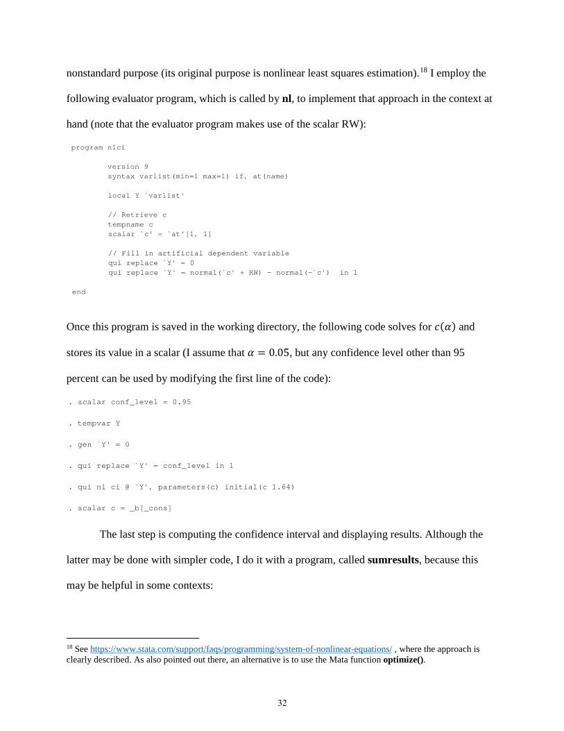
nonstandard purpose (its original purpose is nonlinear least squares estimation).18 I employ the

following evaluator program, which is called by nl, to implement that approach in the context at

hand (note that the evaluator program makes use of the scalar RW):

Once this program is saved in the working directory, the following code solves for 𝑐𝑐(𝛼𝛼) and

stores its value in a scalar (I assume that 𝛼𝛼 = 0.05, but any confidence level other than 95

percent can be used by modifying the first line of the code):

The last step is computing the confidence interval and displaying results. Although the

latter may be done with simpler code, I do it with a program, called sumresults, because this

may be helpful in some contexts:

18 See https://www.stata.com/support/faqs/programming/system-of-nonlinear-equations/ , where the approach is clearly described. As also pointed out there, an alternative is to use the Mata function optimize().

end

qui replace `Y' = normal(`c' + RW) - normal(-`c') in 1 qui replace `Y' = 0 // Fill in artificial dependent variable

scalar `c' = `at'[1, 1] tempname c // Retrieve c local Y `varlist' syntax varlist(min=1 max=1) if, at(name) version 9

program nlci

. scalar c = _b[_cons]

. qui nl ci @ `Y', parameters(c) initial(c 1.64)

. qui replace `Y' = conf_level in 1

. gen `Y' = 0

. tempvar Y

. scalar conf_level = 0.95

32

The results show that the set estimate of the IGE of expected income generated by the

bracketing strategy is highly informative. At the same time, the fact that the confidence interval

for that IGE is rather wide underscores the fact that obtaining satisfactory levels of precision

with that strategy requires samples substantially larger than those that are required to obtain

satisfactory levels of precision with the individual estimators the strategy combines.

7. The igets command

6.1 Syntax

The syntax for the igets command is

igets depvar [ varlist1 ] [ if ] [ in ] [ weight ], instruments(varlist2) sampaux(varname1)

depvaraux(varname2) [ options ]

where varlist1 and varlist2 may contain factor variables, and all types of Stata weights (i.e.,

aweights, fweights, iweights, and pweights) are allowed.

6.2 Options

Required options

instruments(varlist2) specifies the instruments

c(0.05) 1.64530 95% Conf. interval 0.41285 - 0.84288 Set estimate 0.51703 - 0.70578Partially identified IGE of the expectation . sumresults. 10. end 9. di as txt "{hline 60}" 8. di as text _col(6) "c(`alpha')" _col(31) as res %6.5f c 7. di as text _col(6) "`level'% Conf. interval" _col(31) as res %6.5f ci_lb _col(39) as res "- " %6.5f ci_ub 6. di as text _col(6) "Set estimate" _col(31) as res %6.5f lb_pe _col(39) as res "- " %6.5f ub_pe 5. di as text "Partially identified IGE of the expectation" 4. di as txt "{hline 60}" 3. local alpha: di %3.2f `alpha' 2. local alpha = 1 - conf_level 1. local level = 100 * conf_level. program define sumresults. . scalar ci_ub = ub_pe + c * ub_se. scalar ci_lb = lb_pe - c * lb_se

33

sampaux(varname1) specifies the name of an indicator variable identifying the observations

from the auxiliary sample

depvaraux(varname2) specifies the name of the log-parental-income variable, which is the

dependent variable in the auxiliary equation

GMM weight matrix options

wmatrix(wmtype) specifies the weight matrix type; weight matrix type wmtype may be robust

(the default), cluster clustvar, or unadjusted; these types of matrices are as defined in

the Stata manual entry for the gmm command

winitial(iwtype) specifies the initial weight matrix; initial weight matrix iwtype may be

unadjusted, identity (the default), or the name of a Stata matrix; these types of matrices

are as defined in the Stata manual entry for the gmm command

SE/Robust options

vce(vcetype) specifies the type of standard error reported; vcetype may be robust, cluster

clustvar, bootstrap, jackknife, or unadjusted; the default vcetype is based on the

wmtype specified in the wmatrix() option; the types of standard errors, and the rules used

to define the default vcetype, are as described in the Stata manual entry for the gmm

command

Other options

nostandardize requires that, when estimating the elasticity of the expectation, the dependent

variable in the main equation not be standardized by dividing it by its mean (which

normally helps the model converge); the default is to standardize this variable

noinitvalues requires that initial values not be provided for GMM estimation; the default is to

provide initial values

34

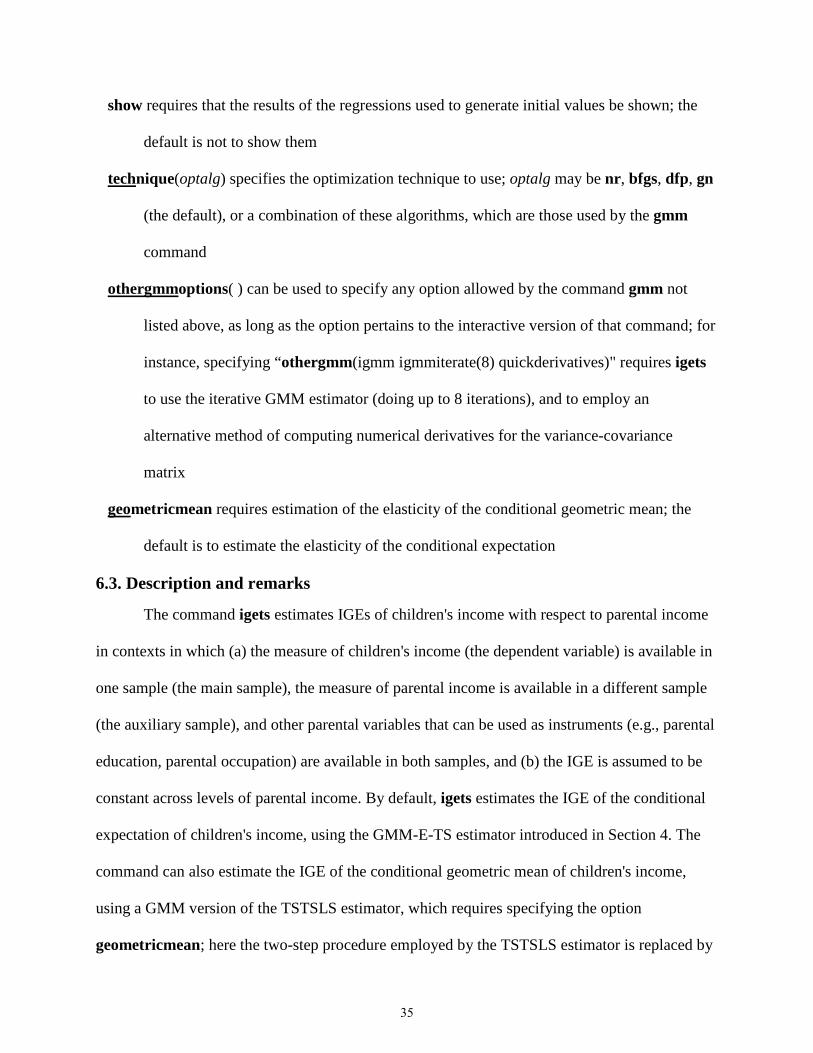
show requires that the results of the regressions used to generate initial values be shown; the

default is not to show them

technique(optalg) specifies the optimization technique to use; optalg may be nr, bfgs, dfp, gn

(the default), or a combination of these algorithms, which are those used by the gmm

command

othergmmoptions( ) can be used to specify any option allowed by the command gmm not

listed above, as long as the option pertains to the interactive version of that command; for

instance, specifying “othergmm(igmm igmmiterate(8) quickderivatives)" requires igets

to use the iterative GMM estimator (doing up to 8 iterations), and to employ an

alternative method of computing numerical derivatives for the variance-covariance

matrix

geometricmean requires estimation of the elasticity of the conditional geometric mean; the

default is to estimate the elasticity of the conditional expectation

6.3. Description and remarks

The command igets estimates IGEs of children's income with respect to parental income

in contexts in which (a) the measure of children's income (the dependent variable) is available in

one sample (the main sample), the measure of parental income is available in a different sample

(the auxiliary sample), and other parental variables that can be used as instruments (e.g., parental

education, parental occupation) are available in both samples, and (b) the IGE is assumed to be

constant across levels of parental income. By default, igets estimates the IGE of the conditional

expectation of children's income, using the GMM-E-TS estimator introduced in Section 4. The

command can also estimate the IGE of the conditional geometric mean of children's income,

using a GMM version of the TSTSLS estimator, which requires specifying the option

geometricmean; here the two-step procedure employed by the TSTSLS estimator is replaced by

35

estimation of a two-equation model by GMM (relying on the approach described in Section 4.4

for the IGE of the expectation).

The program assumes that the names of variables used in estimation have been

harmonized across samples, the auxiliary sample has been appended to the main sample, and

there is an indicator variable, specified in sampaux(varname1), that is coded 0 for the

observations in the main sample and 1 for the observations in the auxiliary sample. It also

assumes that the dependent variable of the main equation, specified by depvar, is the children’s

income when estimating the IGE of the expectation and the logarithm of their income when

estimating the IGE of the geometric mean. In addition, the program assumes that depvar is coded

as 0 (rather than missing) in the auxiliary sample, and that the dependent variable in the auxiliary

equation, specified by option depvaraux(varname2), is coded as 0 (rather than missing) in the

main sample. If this is not the case, the program exits with an error message. At least one

instrument—and as many as desired—need to be specified with the option

instruments(varlist2). Control variables (e.g., a polynomial on children’s age), may be specified

in varilist1 if desired. If one of the samples includes weights (e.g., population weights) and the

other doesn't, weights equal to 1 need to be generated in the latter sample. Otherwise, the

program will exit with an error message if weighted estimation is requested.

The optimization algorithm employed sometimes makes a difference for whether the

model converges or not, and for the time it takes to converge. If the model under estimation has

difficulties converging, users should experiment with the various optimization algorithms

available (and combinations thereof) by using the option technique( ). Combining 15 iterations

of the modified Newton–Raphson algorithm followed by 5 of the Davidon–Fletcher–Powell

algorithm—i.e., specifying technique(nr 15 dfp 5)—has proven particularly useful in some

36

cases. However, estimation with this combination may be much slower than with the default

Gauss–Newton method, so it should only be used if needed.

Specifying the option othergmm(igmm), which requests use of the iterative GMM

estimator, may lead in some cases to estimates that are (non-negligibly) different. These

estimates are likely to be more precise (Hall 2005: Sec. 2.4 and 3.6) than those obtained without

that option. Specifying the option othergmm(igmm igmmiterate(#)), with # > 2 a small

maximum number of iterations (e.g., # = 8), may be a good compromise if the iterative GMM

estimator takes too long to converge.19 The iterative GMM estimator with a maximum of # > 2

iterations can still be expected to be more efficient than the default (for which # = 2). The

wmtype unadjusted and the vcetype unadjusted should in general not be used; they are allowed

by igets mostly because they might serve a pedagogical purpose in some contexts.

The option show displays the estimates generated by the two-step estimator on which the

relevant GMM estimator is based. By default, igets uses these estimates as initial values for the

latter. In addition, when estimating the IGE of the expectation, the dependent variable is divided

by its mean—which affects the intercept of the linear predictor but not the elasticity—as this

often facilitates convergence. Both behaviors can be changed by specifying the options

noinitvalues and nostandardize, respectively. In addition to what is stored by gmm, igets stores

a few macros in e( ), which are listed in the command’s help.

8. Estimating IGEs in the two-sample context: Examples

In this section I present examples of estimation of IGEs in the two-sample context, using

the command igets and a subset of the PSID-based data employed by Mitnik (2017c). Like the

data used in the previous section, the “artificial two-sample” data I use in this section represent

19 Moreover, there is no guarantee that the iterative GMM estimator will converge (e.g., Hall 2005:90).

37

U.S. men and women born between 1966 and 1974. I mostly focus on the estimation of the IGE

of the expectation with the TS-GMM-E estimator, but at the end I also present an example of

estimation of the IGE of the geometric mean with the GMM version of the TSTSLS estimator.

As required by igets, the names of the variables used in estimation are the same across

samples, and the auxiliary sample has been appended to the main sample. Most variables are as

in Section 6, although here I use three additional variables:

c_female Child female c_ln_inc Logarithm of child's family income aux Auxiliary sample cluster Cluster variable

There is one more condition that the data must satisfy for use with igets: The children’s

income variables need to be coded as zero (rather than missing) in the auxiliary sample, and the

parental income variables need to be coded as zero (rather than missing) in the main sample. I

start by reading the data and doing the needed replacements:

In all examples in this section I estimate IGEs with the short-run measure of parental

income based on one year of information, which is what is typically available in the two-sample

context. Like ivpoisson, igets does not accept the survey prefix svy but does allow population

weights, which need to be specified with the data at hand. It also allows to request a weight

matrix that accounts for arbitrary correlation among observations within clusters, and that

cluster-robust standard errors be computed, both of which are also needed with the data I use.20

20 This is needed because of the relationship between the observations in the main and the auxiliary samples (see Mitnik 2017c:22).

. qui replace p_ln_srinc_1y = 0 if aux == 0

. qui replace c_ln_inc = 0 if aux == 1

. qui replace c_inc = 0 if aux == 1

. sysuse twosample_data, clear

38

In all cases I specify the option othergmm(nolog) to save space, but it’s better not to do so (to be

able to examine the iteration log for potential convergence issues).

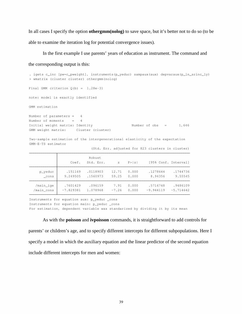
In the first example I use parents’ years of education as instrument. The command and

the corresponding output is this:

As with the poisson and ivpoisson commands, it is straightforward to add controls for

parents’ or children’s age, and to specify different intercepts for different subpopulations. Here I

specify a model in which the auxiliary equation and the linear predictor of the second equation

include different intercepts for men and women:

For estimation, dependent variable was standarized by dividing it by its meanInstruments for equation main: p_yeduc _consInstruments for equation aux: p_yeduc _cons /main_cons -7.829381 1.078968 -7.26 0.000 -9.944119 -5.714642 /main_ige .7601429 .096159 7.91 0.000 .5716748 .9486109 _cons 9.249505 .1560973 59.25 0.000 8.94356 9.55545 p_yeduc .151169 .0118903 12.71 0.000 .1278644 .1744736 Coef. Std. Err. z P>|z| [95% Conf. Interval] Robust (Std. Err. adjusted for 823 clusters in cluster)GMM-E-TS estimatorTwo-sample estimation of the intergenerational elasticity of the expectation

GMM weight matrix: Cluster (cluster)Initial weight matrix: Identity Number of obs = 1,646Number of moments = 4Number of parameters = 4

GMM estimation

note: model is exactly identified

Final GMM criterion Q(b) = 1.28e-31

> wmatrix (cluster cluster) othergmm(nolog). igets c_inc [pw=c_pweight], instruments(p_yeduc) sampaux(aux) depvaraux(p_ln_srinc_1y)

39

In the results table produced by igets, the IGE of the expectation is identified by the term

“ige” while all coefficients from the main equation are identified by the prefix “main”—

although, as we can see in the output from the first two examples, the structure of the table is

different when the equations include additional right-hand variables, beyond those that are

required, and when they don’t. The results show that allowing different intercepts by gender

makes essentially no difference for the estimated IGE, as both models put it at about 0.76.

In the above examples, the computation of cluster-robust standard errors is implied by the

use of a weight matrix of the wmtype cluster. This is so because the default vcetype in igets is

based on the wmtype specified in the wmatrix() option. Now, as the default wmtype is robust,

For estimation, dependent variable was standarized by dividing it by its meanInstruments for equation main: p_yeduc 0b.c_female 1.c_female _consInstruments for equation aux: p_yeduc 0b.c_female 1.c_female _cons _cons -7.753714 1.066004 -7.27 0.000 -9.843043 -5.664386 1.c_female -.0913637 .0750093 -1.22 0.223 -.2383793 .0556519main_other _cons .7572668 .0951306 7.96 0.000 .5708142 .9437193main_ige _cons 9.22405 .1599308 57.68 0.000 8.910591 9.537509 p_yeduc .151244 .0118557 12.76 0.000 .1280071 .1744808 1.c_female .0511126 .0561278 0.91 0.362 -.0588959 .1611211aux Coef. Std. Err. z P>|z| [95% Conf. Interval] Robust (Std. Err. adjusted for 823 clusters in cluster)GMM-E-TS estimatorTwo-sample estimation of the intergenerational elasticity of the expectation

GMM weight matrix: Cluster (cluster)Initial weight matrix: Identity Number of obs = 1,646Number of moments = 6Number of parameters = 6

GMM estimation

note: model is exactly identified

Final GMM criterion Q(b) = 1.01e-31

> wmatrix (cluster cluster) othergmm(nolog). igets c_inc i.c_female [pw=c_pweight], instruments(p_yeduc) sampaux(aux) depvaraux(p_ln_srinc_1y)

40

the default vcetype is also robust. Therefore, had the data been the result of SRS, estimation of

the first model could have been accomplished by the following command:

that is, without having to specify robust standard errors (which are mandatory with the GMM- E-TS estimator). This command only includes the minimum information required by igets: The

children’s income variable, one instrument, the indicator variable identifying the auxiliary

sample, and the parents’ income variable (in logarithms).

In the following example I specify a model in which both parents’ years of education and

its square are used as instruments. As the model converges very slowly with the default

algorithm, I specify the option technique(nr 15 dfp 5). For the reason explained earlier, I also

specify the option othergmm(igmm igmmiterate(8)). The results follow, showing a larger IGE

estimate than in the previous two examples:

. igets c_inc, instruments(p_yeduc) sampaux(aux) depvaraux(p_ln_srinc_1y)

For estimation, dependent variable was standarized by dividing it by its meanInstruments for equation main: p_yeduc c.p_yeduc#c.p_yeduc _consInstruments for equation aux: p_yeduc c.p_yeduc#c.p_yeduc _cons /main_cons -8.734743 1.129218 -7.74 0.000 -10.94797 -6.521516 /main_ige .8392476 .1008351 8.32 0.000 .6416145 1.036881 _cons 8.575028 .4330375 19.80 0.000 7.726291 9.423766 c.p_yeduc#c.p_yeduc -.0045586 .0027657 -1.65 0.099 -.0099792 .000862 p_yeduc .2641736 .0691984 3.82 0.000 .1285472 .3998 Coef. Std. Err. z P>|z| [95% Conf. Interval] Robust (Std. Err. adjusted for 823 clusters in cluster)GMM-E-TS estimatorTwo-sample estimation of the intergenerational elasticity of the expectation

GMM weight matrix: Cluster (cluster)Initial weight matrix: Identity Number of obs = 1,646Number of moments = 6Number of parameters = 5

GMM estimation

Final GMM criterion Q(b) = .0018108

note: iterative GMM parameter vector converged

> wmatrix (cluster cluster) othergmm(igmm igmmiterate(8) nolog) tech(nr 15 dfp 5). igets c_inc [pw=c_pweight], instruments(c.p_yeduc c.p_yeduc#c.p_yeduc) sampaux(aux) depvaraux(p_ln_srinc_1y)

41

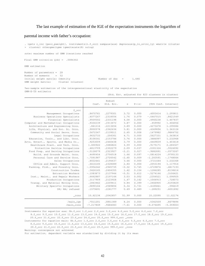
The last example of estimation of the IGE of the expectation instruments the logarithm of

parental income with father’s occupation:

For estimation, dependent variable was standarized by dividing it by its meanWarning: convergence not achieved 20.f_occ 21.f_occ 22.f_occ 23.f_occ 24.f_occ 25.f_occ 999.f_occ _cons 8.f_occ 9.f_occ 10.f_occ 11.f_occ 13.f_occ 14.f_occ 15.f_occ 16.f_occ 17.f_occ 18.f_occ 19.f_occInstruments for equation main: 0b.f_occ 1.f_occ 2.f_occ 3.f_occ 4.f_occ 5.f_occ 6.f_occ 7.f_occ 20.f_occ 21.f_occ 22.f_occ 23.f_occ 24.f_occ 25.f_occ 999.f_occ _cons 8.f_occ 9.f_occ 10.f_occ 11.f_occ 13.f_occ 14.f_occ 15.f_occ 16.f_occ 17.f_occ 18.f_occ 19.f_occInstruments for equation aux: 0b.f_occ 1.f_occ 2.f_occ 3.f_occ 4.f_occ 5.f_occ 6.f_occ 7.f_occ /main_cons -7.217849 .9484083 -7.61 0.000 -9.076695 -5.359003 /main_ige .7011201 .0851389 8.24 0.000 .5342509 .8679894 _cons 10.62134 .2042857 51.99 0.000 10.22095 11.02174 DK; NA; refused .1579691 .2281777 0.69 0.489 -.289251 .6051892 Military Specific Occupations .0890164 .2589856 0.34 0.731 -.4185861 .596619 Transp. and Material Moving Occs. .1863462 .2209411 0.84 0.399 -.2466905 .6193829 Production Occupations .3117909 .2123928 1.47 0.142 -.1044913 .728073 Inst., Maint., and Repair Workers .6662887 .2197166 3.03 0.002 .2356521 1.096925 Extraction Workers -.1083873 .2137944 -0.51 0.612 -.5274166 .3106421 Construction Trades .3426165 .2404355 1.42 0.154 -.1286285 .8138614 Farming, Fish., and Forestry Occs. -.0956342 .2945735 -0.32 0.745 -.6729876 .4817193 Office and Admin. Support Occs. .6616165 .2328089 2.84 0.004 .2053194 1.117914 Sales Occupations .8022661 .2194437 3.66 0.000 .3721644 1.232368 Personal Care and Service Occs. -.7091987 .2726542 -2.60 0.009 -1.243591 -.1748064 Build. and Grounds Maint. Occs. .4490454 .2706518 1.66 0.097 -.0814224 .9795133 Food Prep. and Serving Occupations -.5128079 .2323927 -2.21 0.027 -.9682891 -.0573267 Protective Service Occupations .4813709 .2302279 2.09 0.037 .0301326 .9326092 Healthcare Pract. and Tech. Occs. 1.600922 .3486824 4.59 0.000 .9175171 2.284327Arts, Entert., Sports, and Media Oc.. .9253009 .2440438 3.79 0.000 .4469839 1.403618 Education, Train., and Libr. Occs. .8108341 .2153786 3.76 0.000 .3886997 1.232968 Legal Occupations .9632733 .204361 4.71 0.000 .5627331 1.363814 Community and Social Servs. Occs. .5672367 .2139011 2.65 0.008 .1479982 .9864752 Life, Physical, and Soc. Sc. Occs. .9000578 .2362636 3.81 0.000 .4369896 1.363126 Architecture and Engineering Occs. .861216 .2213654 3.89 0.000 .4273478 1.295084Computer and Mathematical Occupations .9330239 .2413472 3.87 0.000 .459992 1.406056 Financial Specialists .9509302 .2331198 4.08 0.000 .4940238 1.407837 Business Operations Specialists .4077267 .2318554 1.76 0.079 -.0467015 .8621549 Management Occupations .8470761 .2279301 3.72 0.000 .4003414 1.293811 f_occ Coef. Std. Err. z P>|z| [95% Conf. Interval] Robust (Std. Err. adjusted for 823 clusters in cluster)GMM-E-TS estimatorTwo-sample estimation of the intergenerational elasticity of the expectation

GMM weight matrix: Cluster (cluster)Initial weight matrix: Identity Number of obs = 1,646Number of moments = 52Number of parameters = 28

GMM estimation

Final GMM criterion Q(b) = .0086302

note: maximum number of GMM iterations reached

> cluster) othergmm(igmm igmmiterate(8) nolog). igets c_inc [pw=c_pweight], instruments(i.f_occ) sampaux(aux) depvaraux(p_ln_srinc_1y) wmatrix (cluster

42

As in all other examples in Section 6 and in this section in which I used multiple

instruments with a GMM estimator, here I requested that the iterative GMM estimator, with up

to 8 iterations, be used (rather than the default GMM estimator, where the number of iterations is

2). Unlike in all previous cases, however, in this case the GMM iterative estimator did not

converge in 8 iterations, and this is noted in two places in the output: Indirectly at the top, where

there is a note saying “maximum number of GMM iterations reached,” and directly at the

bottom, where there is a warning saying “convergence not achieved.” This is fully

unproblematic. Like the default estimator, any GMM iterative estimator based on # > 2 iterations

is consistent; moreover, as already indicated, it is likely more efficient that the default estimator

in finite samples.

As I am using data that are “artificially two-sample,” and the original data include a

measure of long-run parental income, the long-run IGE of the expectation can be estimated with

the PPML estimator. This estimate is the one I reported in Section 6, i.e. 0.60 (see the first

example in that section). Therefore, examining the results obtained in this section, we see that (a)

as expected, all IGE estimates produced by the GMM-E-TS estimator are upper-bound estimates,

and (b) as with the GMM-IVP estimator in the one-sample context, in the two-sample context the

estimate using father’s occupation as instrument, 0.70, provides the tightest upper bound, while

those obtained by using parents’ years of education, alone and as second degree polynomial, put

the IGE at 0.76 and 0.84, respectively.

I finish the section with an example of estimation of the conventional IGE, in which I use

parents’ years of education as instrument. Estimation of the conventional IGE is achieved by

substituting the logarithm of children’s income for children’s income as outcome variable, and

43

specifying the option geometricmean. I also specify the option show, just to show that, with a

single instrument, igets reproduces the point estimate obtained with the TSTSLS estimator.

The estimate of 0.91 is larger than the log-run estimate of the conventional IGE obtained with

Instruments for equation main: p_yeduc _consInstruments for equation aux: p_yeduc _cons /main_cons 1.060185 1.221688 0.87 0.386 -1.334279 3.454649/main_ige_gm .9117561 .1087229 8.39 0.000 .6986632 1.124849 _cons 9.249505 .1560973 59.25 0.000 8.94356 9.55545 p_yeduc .151169 .0118903 12.71 0.000 .1278644 .1744736 Coef. Std. Err. z P>|z| [95% Conf. Interval] Robust (Std. Err. adjusted for 823 clusters in cluster)GMM version of the TSTSLS estimatorTwo-sample estimation of the intergenerational elasticity of the geometric mean

GMM weight matrix: Cluster (cluster)Initial weight matrix: Identity Number of obs = 1,644Number of moments = 4Number of parameters = 4

GMM estimation

note: model is exactly identified

Final GMM criterion Q(b) = 1.20e-31

Joint estimation by GMM

_cons 1.060185 1.180002 0.90 0.369 -1.255999 3.376369p_ln_srinc_1y_hat .9117561 .1050486 8.68 0.000 .7055599 1.117952 c_ln_inc Coef. Std. Err. t P>|t| [95% Conf. Interval] Robust

Root MSE = .77855 R-squared = 0.1325 Prob > F = 0.0000 F(1, 819) = 75.33Linear regression Number of obs = 821

(sum of wgt is 3.1455e+04)Second-step regression

_cons 9.249505 .1562873 59.18 0.000 8.942735 9.556275 p_yeduc .151169 .0119048 12.70 0.000 .1278015 .1745364 p_ln_srin~1y Coef. Std. Err. t P>|t| [95% Conf. Interval] Robust

Root MSE = .66842 R-squared = 0.1996 Prob > F = 0.0000 F(1, 821) = 161.24Linear regression Number of obs = 823

(sum of wgt is 3.1493e+04)First-step regression

Generating initial values

> cluster) geometricmean show othergmm(nolog). igets c_ln_inc [pw = c_pweight], instruments(p_yeduc) sampaux(aux) depvaraux(p_ln_srinc_1y) wmatrix (cluster

44

the underlying data and the OLS estimator, which puts that IGE at 0.70. This is in agreement

with the standard approach in the literature, which treats TSTSLS estimates as upper-bound

estimates.

9. Concluding remarks

I have explained how to use Stata official commands to estimate the IGE of the

expectation in the one-sample context, employing the PPML and GMM-IVP estimators, and how

to construct confidence intervals for the partially identified IGE when the estimates obtained

with those estimators are combined to generate a set estimate. I have also introduced the user-

written program igets, which allows to estimate IGEs in the two-sample context, and have shown

how to use it to estimate the IGE of the expectation with the GMM-E-TS estimator. By

providing a suite of estimators and Stata commands to estimate the IGE of the expectation in all

situations in which the IGE of the geometric mean has been estimated by mobility scholars, I

hope to contribute to the replacement of the latter by the former as the workhorse

intergenerational elasticity.

10. References

Aaronson, David and Bhashkar Mazumder. 2008. “Intergenerational Economic Mobility in the US: 1940 to 2000.” Journal of Human Resources 43(1): 139-172.

Björklund, Anders and Markus Jäntti. 2000. “Intergenerational Mobility of Socio-Economic Status in Comparative Perspective.” Nordic Journal of Political Economy 26: 3-32.

Böhlmark, Anders and Matthew Lindquist. 2006. “Life-Cycle Variations in the Association between Current and Lifetime Income: Replication and Extension for Sweden,” Journal of Labor Economics, 24(4): 879–896.

Black, Sandra and Paul Devereux. 2011. “Recent Developments in Intergenerational Mobility.” Handbook of Labor Economics, Volume 4b, edited by David Card and Orley Ashenfelter. Amsterdam: Elsevier.

Bloome, Deirdre. 2015. “Income Inequality and Intergenerational Income Mobility in the United States.” Social Forces, 93(3): 1047-1080.

Bloome, Deirdre and Western. 2011. “Cohort Change and Racial Differences in Educational and Income Mobility.” Social Forces, 90(2): 375-395.

45

Bratsberg, Bernt, Knut Røed, Oddbjørn Raaum, Robin Naylor, Markus Jäntti, Tor Eriksson and Eva Österbacka. 2007. “Nonlinearities in Intergenerational Earnings Mobility. Consequences for Cross-Country Comparisons.” The Economic Journal, 117 (March) C72-C92.

Carroll, Raymond, David Ruppert, Leonard Stefanski, and Ciprian Crainiceanu. 2006. Measurement Error in Nonlinear Models: A Modern Perspective (second edition). Boca Raton: Chapman & Hall/CRC.

Chadwick, Laura and Gary Solon. 2002. “Intergenerational Income Mobility among Daughters.” The American Economic Review 92(1): 335-344.

Corak, Miles. 2006. “Do Poor Children Become Poor Adults? Lessons from a Cross Country Comparison of Generational Earnings Mobility.” IZA Discussion Paper No. 1993, IZA.

Corak, Miles. 2013. “Income Inequality, Equality of Opportunity, and Intergenerational Mobility.” Journal of Economic Perspectives 27 (3):79-102.

Gourieroux, C, A. Monfort and A. Trognon. 1984. “Pseudo Maximum Likelihood Methods: Theory.” Econometrica 52(3): 681-700.

Grawe, Nathan. 2003. “Life Cycle Bias in the Estimation of Intergenerational Earnings Persistence." Analytical Studies Branch Research Paper Series 2003207e, Statistics Canada, Analytical Studies Branch.

Haider, Steven and Gary Solon. 2006. “Life-Cycle Variation in the Association between Current and Lifetime Earnings.” American Economic Review 96(4): 1308-1320.

Hall, Alastair. 2005. Generalized Method of Moments. Oxford: Oxford University Press. Hardin, James. 2002. “The Robust Variance Estimator for Two-Stage Models.” The Stata

Journal 2(3): 253-266. Hertz, Tom. 2005. “Rags, Riches and Race: The Intergenerational Economic Mobility of Black

and White Families in the United States.” In Unequal Chances. Family Background and Economic Success, edited by Samuel Bowles, Herbert Gintis, and Melissa Osborne Groves. New York, Princeton and Oxford: Russell Sage and Princeton University Press.

Hertz, Tom. 2007. “Trends in the Intergenerational Elasticity of Family Income in the United States.” Industrial Relations 46(1): 22-50.

Imbens, Guido and Charles Manski. 2004. “Confidence Intervals for Partially Identified Parameters.” Econometrica 72(6): 1845-1857.

Inoue, Atsushi and Gary Solon. 2010. “Two-Sample Instrumental Variables Estimators.” The Review of Economics and Statistics 92(3):557-561.

Jäntti, Markus and Stephen Jenkins. 2015. “Income Mobility.” In Handbook of Income Distribution (Vol. 2A), edited by Anthony Atkinson and François Bourguignon. Amsterdam: Elsevier.

Jerrim, John, Álvaro Choi, and Rosa Simancas. 2016. “Two-Sample Two-Stage Least Squares (TSTSLS) Estimates of Earnings Mobility: How Consistent Are They?” Survey Research Methods 10(2):85-102.

46

Landersø, Rasmus and James Heckman. 2016. “The Scandinavian Fantasy: The Sources of Intergenerational Mobility in Denmark and the U.S.” NBER Working Paper 22465.

Manski, Charles. 2003. Partial Identification of Probability Distributions. New York: Springer-Verlag.

Mazumder, Bhashkar. 2001. “The Miss-measurement of Permanent Earnings: New Evidence from Social Security Earnings Data.” Federal Reserve Bank of Chicago Working Paper 2001-24.

Mazumder, Bhashkar. 2005. “Fortunate Sons: New Estimates of Intergenerational Mobility in the United States Using Social Security Earnings Data.” The Review of Economics and Statistics 87(2): 235-255.

Mazumder, Bhashkar. 2016. “Estimating the Intergenerational Elasticity and Rank Association in the United States: Overcoming the Current Limitation of Tax Data.” In Inequality: Causes and Consequences, edited by Lorenzo Cappellari, Solomon Polacheck, and Konstantinos Tatsiramos. Bingley: Emerald.

Mullahy, John. 1997. “Instrumental-Variable Estimation of Count Data Models: Applications to Models of Cigarette Smoking Behavior.” Review of Economics and Statistics 79(4): 586-593.

Mayer, Susan E., and Leonard Lopoo. 2008. “Government Spending and Intergenerational Mobility.” Journal of Public Economics 92: 139-58.

Mitnik, Pablo. 2017a. “Estimating the Intergenerational Elasticity of Expected Income with Short-Run Income Measures: A Generalized Error-in-Variables Model.” Stanford Center on Poverty and Inequality Working Paper.

Mitnik, Pablo. 2017b. “Intergenerational Income Elasticities, Instrumental Variable Estimation, and Bracketing Strategies.” Stanford Center on Poverty and Inequality Working Paper.

Mitnik, Pablo. 2017c. “Two-Sample Estimation of the Intergenerational Elasticity of Expected Income.” Stanford Center on Poverty and Inequality Working Paper.

Mitnik, Pablo, Victoria Bryant, Michael Weber and David Grusky. 2015. “New Estimates of Intergenerational Mobility Using Administrative Data.” SOI Working Paper, Statistics of Income Division, Internal Revenue Service.

Mitnik, Pablo and David Grusky. 2017. The Intergenerational Elasticity of What? A Call for Redefining the Workhorse Measure of Economic Mobility.” Stanford Center on Poverty and Inequality Working Paper.

Mulligan, Casey. 1997. Parental Priorities and Economic Inequality. Chicago: University of Chicago Press.

Murphy, Kevin and Robert Topel. 1985. “Estimation and Inference in Two-Step Econometric Models.” Journal of Business & Economic Statistics 3(4): 370-379.

Newey, Whitney. 1984. “A Method of Moments Interpretation of Sequential Estimators.” Economics Letters 14(2-3):201-206.

Ng, Irene. 2007. “Intergenerational Income Mobility in Singapore,” The B.E. Journal of Economic Analysis & Policy 7(2): Article 3.

47

Nybom, Martin and Jan Stuhler. 2016. “Heterogeneous Income Profiles and Life-Cycle Bias in Intergenerational Mobility Estimation.” The Journal of Human Resources 15(1): 239-268.

Petersen, Trond. 2017. “Multiplicative Models for Continuous Dependent Variables: Estimation on Unlogged versus Logged Form.” Sociological Methodology 47:113-164.

Reiss, Peter. 2016, “Just How Sensitive are Instrumental Variable Estimates?”. Foundations and Trends in Accounting 10(2-4): 204–237.

Santos Silva, J. M. C. and Silvana Tenreyro. 2006. "The Log of Gravity." The Review of Economics and Statistics 88(4): 641-658.

Santos Silva, J. M. C. and Silvana Tenreyro. 2011. “Further Simulation Evidence on the Performance of the Poisson Pseudo-maximum Likelihood Estimator.” Economics Letters 112: 220-222.

Solon, Gary. 1992. “Intergenerational Income Mobility in the United States.” American Economic Review 82(3): 393-408.

Solon, Gary. 1999. “Intergenerational Mobility in the Labor Market.” Handbook of Labor Economics, Volume 3A, edited by Orley C. Ashenfelter and David Card. Amsterdam: Elsevier.

Solon, Gary. 2004. “A Model of Intergenerational Mobility Variation over Time and Place.” In Generational Income Mobility in North America in Europa, edited by Miles Corak. Cambridge: Cambridge University Press.

Stoye, Jörg. 2009. “More on Confidence Regions for Partially Identified Parameters.” Econometrica 77(4):1299–1315.

Tamer, Elie. 2010. “Partial Identification in Econometrics.” The Annual Review of Economics 2: 167-195.

Terza, Joseph, Anirban Basu, Paul J. Rathouz. 2008. “Two-Stage Residual Inclusion Estimation: Addressing Endogeneity in Health Econometric Modeling.” Journal of Health Economics 27(3):531-543.

Windmeijer, F. A. G. and J. M. C. Santos Silva. 1997. “Endogeneity in Count Data Models: An Applications to Demand for Health Care.” Journal of Applied Econometrics 12: 281-294.

Winkelmann, Rainer. 2008. Econometric Analysis of Count Data. Berlin: Springer-Verlag. Wooldridge, Jeffrey. 1999. “Quasi-Likelihood Methods for Count Data.” In Handbook of

Applied Econometrics Volume II: Microeconomics, edited by M. Hashem Pesaran and Peter Schmidt. Blackwell Publishing.

Wooldridge, Jeffrey. 2002. Econometric Analysis of Cross Section and Panel Data. Cambridge, Mass: The MIT Press.

Zimmerman, David J. 1992. “Regression toward Mediocrity in Economic Stature.” American Economic Review 82 (3), pp. 409-429.

48