esu-services - description of life cycle impact...

Schaffhausen, 15. June 2020

15.06.20 08:33 https://esuservices-my.sharepoint.com/personal/mitarbeiter1_esuservices_onmicrosoft_com/Documents/files/Vorlagen/ESU-Description-of-LCIAmethods.docx

Niels Jungbluth Dr. sc. Techn. Dipl. Ing. TU CEO www.esu-services.ch

ESU-services GmbH Vorstadt 14 CH-8200 Schaffhausen

T +41 44 940 61 32 F +41 44 940 67 94 [email protected]

Description of life cycle impact assessment methods Supplementary information for tenders

ESU-services Ltd.

Vorstadt 14

CH-8200 Schaffhausen

UID: CHE-112.959.660

Commercial registry by the canton of Schaffhausen: CHE-112.959.660

VAT number Switzerland: 649 962

https://www.uid.admin.ch/Detail.aspx?uid_id=CHE-112.959.660

https://sh.chregister.ch/cr-portal/auszug/auszug.xhtml?uid=CHE-112.959.660

Description of life cycle impact assessment methods 1

© ESU-services Ltd.

Imprint

Citation Niels Jungbluth (2020) Description of life cycle impact assessment methods. ESU-services

Ltd., Schaffhausen, Switzerland, http://esu-services.ch/address/tender/

Contractor

ESU-services Ltd., fair consulting in sustainability

Vorstadt 14, CH-8200 Schaffhausen

www.esu-services.ch

Phone 0041 44 940 61 32

[email protected]

Commissioner

About us

ESU-services Ltd. has been founded in 1998. Its core objectives are consulting, coaching,

training and research in the fields of life cycle assessment (LCA), carbon footprints, water

footprint in the sectors energy, civil engineering, basic minerals, chemicals, packaging,

telecommunication, food and lifestyles. Fairness, independence and transparency are

substantial characteristics of our consulting philosophy. We work issue-related and

accomplish our analyses without prejudice. We document our studies and work

transparency and comprehensibly. We offer a fair and competent consultation, which

makes it for the clients possible to control and continuously improve their environmental

performance. The company worked and works for various national and international

companies, associations and authorities. In some areas, team members of ESU-services

performed pioneering work such as development and operation of web based LCA

databases or quantifying environmental impacts of food and lifestyles.

Copyright All content provided in this report is copyrighted, except when noted otherwise. Such

information must not be copied or distributed, in whole or in part, without prior written

consent of ESU-services Ltd. or the customer. This report is provided on the website

www.esu-services.ch and/or the website of the customer. A provision of this report or of

files and information from this report on other websites is not permitted. Any other means of

distribution, even in altered forms, require the written consent. Any citation naming ESU-

services Ltd. or the authors of this report shall be provided to the authors before publication

for verification.

Liability Statement

This report has been prepared by with great care, using available, up-to-date and

appropriate databases, within the framework of the contractual agreement with the client,

taking into account the agreement regarding resources used. Nevertheless, the authors or

their organizations do not accept liability for any loss or damage arising from the use

thereof. Using the given information is strictly your own responsibility. Any publication of the

contents of this report which only partially presents the results and conclusions thereof and

which does not constitute an integral part of the overall report is not permitted. In particular,

such publications may not cite this report as a source or otherwise be linked to this report or

ESU-services. We disclaim any responsibility towards the client and third parties for claims

outside the above-mentioned scope.

Version 15.06.20 08:33

https://esuservices-

my.sharepoint.com/personal/mitarbeiter1_esuservices_onmicrosoft_com/Documents/files/V

orlagen/ESU-Description-of-LCIAmethods.docx

http://esu-services.ch/address/tender/

http://www.esu-services.ch/

mailto:[email protected]

http://www.esu-services.ch/



Contents

1 OVERVIEW 4

2 SINGLE ISSUES 6

2.1 Cumulative Energy Demand (CED) ................................................................................................ 6

2.2 Cumulative Exergy Demand ............................................................................................................ 6

2.3 Global Warming Potential 2013 (GWP) ........................................................................................... 6

2.4 Indicators for water use and consumption (water footprint) ............................................................ 8 2.4.1 Definitions .............................................................................................................................. 8 2.4.2 AWARE-method (2018) ...................................................................................................... 10 2.4.3 Former assessment methods .............................................................................................. 12

3 IMPACT WORLD+ (2019) 16

3.1 What is ImpactWorld+? ................................................................................................................. 16

3.2 How does ImpactWorld+ differ from other LCIA methods? ........................................................... 16

3.3 Features ........................................................................................................................................ 16

3.4 Conclusions ................................................................................................................................... 17

4 PEF - EUROPEAN ENVIRONMENTAL FOOTPRINT METHOD (2018) 17

4.1 Climate Change ............................................................................................................................. 18

4.2 Ozone depletion ............................................................................................................................ 18

4.3 Ionising radiation - human health .................................................................................................. 18

4.4 Photochemical ozone formation - human health ........................................................................... 18

4.5 Respiratory inorganics ................................................................................................................... 18

4.6 Non-cancer human health effects ................................................................................................. 18

4.7 Cancer human health effects ........................................................................................................ 19

4.8 Acidification terrestrial and freshwater .......................................................................................... 19

4.9 Eutrophication freshwater .............................................................................................................. 19

4.10 Eutrophication marine.................................................................................................................... 19

4.11 Eutrophication terrestrial................................................................................................................ 19

4.12 Ecotoxicity freshwater.................................................................................................................... 19

4.13 Land Use ....................................................................................................................................... 19

4.14 Water scarcity ................................................................................................................................ 19

4.15 Resource use, energy carriers ...................................................................................................... 20

4.16 Resource use, mineral and metals ................................................................................................ 20

5 ENVIRONMENTAL PRODUCT DECLARATION (ENVIRONDEC) (2018) 20

5.1 Default indicators ........................................................................................................................... 20

5.2 Use of ressources .......................................................................................................................... 22

5.3 Waste production and output flows ............................................................................................... 22

5.4 Additional indicators ...................................................................................................................... 22

6 SWISS ENVIRONMENTAL FOOTPRINT INDICATORS (2018) 22

7 ENVIRONMENTAL IMPACTS ACCORDING TO RECIPE (2016) 24

7.1 ReCiPe 2016 ................................................................................................................................. 24

7.2 ReCiPe 2008 (partly outdated) ...................................................................................................... 24



8 SWISS ECOLOGICAL SCARCITY METHOD 2013 (ECO-POINTS 2013) 25

9 ILCD RECOMMENDED LIFE CYCLE IMPACT ASSESSMENT METHODS (2010, OUTDATED) 28

9.1 Overview ........................................................................................................................................ 28

9.2 Long-term emissions ..................................................................................................................... 31

9.3 Abiotic resource depletion ............................................................................................................. 31

9.4 Ecotoxicity freshwater.................................................................................................................... 31

10 IMPACT 2002+ (OUTDATED) 32

10.1 Introduction .................................................................................................................................... 32

10.2 Midpoint indicators ......................................................................................................................... 32

10.3 Endpoint indicators ........................................................................................................................ 32

10.4 Normalization ................................................................................................................................. 33

10.5 Weighting ....................................................................................................................................... 33

11 ECOLOGICAL SCARCITY 2006 (OUTDATED) 33

12 CML 2001 (OUTDATED) 34

12.1 Acidification (kg SO2 eq) ................................................................................................................ 34

12.2 Eutrophication (kg PO43- eq) .......................................................................................................... 34

12.3 Photochemical oxidation (kg ethane eq) – average European ozone concentration change ....... 34

12.4 Land competition (m2a) ................................................................................................................. 34

13 ECO-INDICATOR 99 (OUTDATED) 34

14 REFERENCES 35



1 Overview An essential aspect of the life cycle assessment is the combination of different environmental impacts

(such as the greenhouse effect or eutrophication) into one indicator. Various evaluation methods are

available for this purpose, which differ in scope and procedure for characterisation and weighting.

Tab. 1.1 shows a comparison of different indicators for the evaluation. Methods such as cumulative

energy demand, water footprint or CO2 footprint only consider one selected environmental area at a

time. Fully aggregating methods such as the method of ecological scarcity (environmental impact

points), on the other hand, combine a large number of different environmental impacts into one point

value (see Jungbluth et al. 2011a; Jungbluth et al. 2011b for further explanations).



Tab. 1.1 Overview on LCIA methods

© ESU-services Ltd. (2019) One environmental issue Several issues

LCIA method:

Impact category

Energy,non-renewable

Energy, renewable

Ore and minerals

Water depletion

Biotic resources

Land occupation

Land-transformation

Only CO2

Climate change incl. CO2

Ozone depletion

Human toxicity

Particulate matter formation

Photochemical ozone formation

Ecotoxicity

Acidification

Eutrophication

Persistant organic pollutants

Odours

Noise

Ionising radiation

Endocrine disruptors

Accidents

Wastes

Littering

Salinisation

Biodiversity loss

Erosion

Reference GLO GLO GLO CH GLO RER GLO GLO

Publication 2007 2013 1996 2013 2016 2018 2019 2009

Damage assessment partly

Normalization GLO CH GLO GLO

Weighting

ReCiPeEcological

footprint

Ecological

scarcity

ImpactWorld+,

Midpoint

Environmental

Footprint

(PEF)

Planetary

Boundaries

Fra

mew

ork

Cumulative

Energy

Demand

Carbon

footprint

Resourc

es

Em

issio

ns

Oth

ers



2 Single issues

2.1 Cumulative Energy Demand (CED)

The CED (implementation according to Frischknecht et al. 2007b) describes the consumption of fossil,

nuclear and renewable energy sources along the life cycle of a good or a service. This includes the

direct uses as well as the indirect or grey consumption of energy due to the use of, e.g. plastic or wood

as construction or raw materials. This method has been developed in the early seventies after the first

oil price crisis and has a long tradition (Boustead & Hancock 1979; Pimentel 1973). A CED assessment

can be a good starting point in an assessment due to its simplicity in concept and its comparability

with CED results in other studies. In this study, the CED indicator is used as a resource indicator.

The following two CED indicators are calculated:

• CED, total

• CED, non-renewable (MJ-eq.) – fossil and nuclear

• CED, renewable (MJ-eq.) – hydro, solar, wind, geothermal, biomass

2.2 Cumulative Exergy Demand

The cumulative exergy demand (CExD) is based on the method developed for the ecoinvent database

(Bösch et al. 2007; European Commission et al. 2010; Frischknecht et al. 2007b). The cumulative

exergy demand is split into different subcategories to discriminate between different types of

renewable and non-renewable origins. They are listed in Tab. 2.1.

Tab. 2.1 Explanation for the sub-categories of the cumulative exergy demand

Sub-category Explanation

Non-renewable, fossil Exergy content of fossil resources like coal, crude oil, natural gas, peat and

others (chemical energy)

Non-renewable, nuclear Energy from uranium converted in the technical system (nuclear energy)

Renewable, kinetic (wind) Energy from wind converted in the technical system (kinetic energy)

Renewable, solar Energy from the sun converted in the technical system (radiative energy)

Renewable, potential (water) Energy from hydropower reservoir (potential energy)

Non-renewable, primary forest Exergy content of wood from primary forests (chemical energy)

Renewable, biomass Exergy content of other wood sources (chemical energy)

Renewable, water Exergy content of extracted fresh water minus released water (chemical energy)

Non-renewable, metals Exergy content of metal resources (chemical energy)

Non-renewable, minerals Exergy content of mineral resources (chemical energy)

2.3 Global Warming Potential 2013 (GWP)

The Global Warming Potential (GWP), commonly referred to with the popular term carbon footprint

(CF), calculates the radiative forcing over a 100 year time horizon. It assesses the potential impact of

different gaseous emissions on climate change (IPCC 2013). Climate change is a global problem. It

leads to several different direct and indirect effects on human health, man-made infrastructures and

environmental damages such as:

• warmer or colder temperature at certain places and times

• changes in the amount, annual distribution and magnitude of rainfalls and snowfalls

• changes in the magnitude of wind velocities



• melting of glaciers leading to disappearance of permafrost areas, higher sea level and changes in

salinity

• acidification of oceans due to higher concentration of carbonic acid

• changes in local or global climate phenomena such as the gulf stream, monsoon seasons, etc.

There is no mechanism to clean up these damages and emissions will today emissions will lead to long

lasting changes in the climate system of the earth.

The residence time of the substances in the atmosphere and the expected immission design are

considered to determine the global warming potentials. The potential impact of the emission of one

kilogram of a greenhouse gas is compared to the potential impact of the emission of one kilogram CO2

resulting in kg CO2-equivalents (kg CO2-eq).

The gases with the greatest global warming impact are CO2, CH4 (methane) and N2O (nitrous oxide).

In addition, various chlorinated and fluorinated hydrocarbons (CFCs, HCFCs, HFCs, PFCs) and SF6

have a direct radiative forcing effect. While the global warming impact of the latter substances per

kilogram can be several thousand times greater than that of CO2, their contribution to the overall

emissions inventory is often small.

The global warming potentials can be determined applying different time horizons (20, 100 and 500

years). The short integration period of 20 years is relevant because a limitation of the gradient of

change in temperature is required to secure the adaptation ability of terrestrial ecosystems. The long

integration time of 500 years is about equivalent with the integration until infinity. This allows

monitoring the overall change in temperature and thus the overall sea level rise, etc. In this study a

time horizon of 100 years is chosen, which is also used in the Kyoto protocol.

There are specific effects of emissions in high altitude, which lead to a higher contribution of aviation

to the problem of climate change than just the emission of CO2 from burning aviation fuels. The exact

relevance is subject to scientific debate, but there is a consensus that aircrafts have an impact that is

higher than just their contribution due to the direct CO2. The gap between this scientific knowledge

on the one side and the missing of applicable GWP (global warming potential) factors on the other

side is an important shortcoming for life cycle assessment or carbon footprint studies which aim to

cover all relevant environmental impacts of the services or products investigated (Jungbluth 2013). As

transportation by aircraft has a high relevance in this assessment, some sensitivity analyses with an

adaptation of the IPCC 2013 methodology are included in the assessment. Therefore a factor for the

RFI (radiative forcing index) is included. This better represents the state of the art concerning the

accounting of specific aircraft emissions. For the time being an RFI of 2 on total aircraft CO2 (or 5.2

for the CO2 emissions in the higher atmosphere) is the best-practice approach because it is based on

recent scientific publications, this basic literature cannot be misinterpreted. Furthermore it is also

recommend by some political institutions (Jungbluth 2013).

Tab. 2.2 shows typical reference values for products and services causing an global warming potential

of 1 kg CO2-eq. The IPCC Method with the RFI Factor was used.



Tab. 2.2 Reference values for products and services causing 1kg CO2-eq

2.4 Indicators for water use and consumption (water footprint)

2.4.1 Definitions

A range of different terms is used in the context of water use and water consumption. As a base for

the following, methodical discussions, some basic terms are listed, and their definition is harmonised

in Tab. 2.3.

The distinction between water consumption and water use is important. While the water use includes

the water input and all types of water uses (e.g. cooling, turbinating, irrigation etc.), the water

consumption describes only the amount of water that is lost to a watershed because of the production

of a good or the cultivation of crops. Water consumption is sometimes also called “net water use” or

“net water withdrawal”. The water consumption itself can be specified according to the type and origin

of the water source. It is sometimes differentiated into blue, green and grey water. The definition of

these types of water can vary slightly among the different studies and according to their scope and

system boundaries.

The analysis of the water consumption concentrates mainly on the quantity of the water. The

degradation of the water quality is assessed in LCA in separate impact categories (e.g. ecotoxicity or

eutrophication). Despite that is the grey water consumption is an indicator for the harmfulness of the

substances emitted, although not damage oriented.

5672 litres of tapwater from Switzerland

11.7 centimeters road, used for one year

1.0 kilograms of fossil CO2, directly emitted

0.03 kilograms of fossil methane, directly emitted

1.4 litres crude oil produced, with transport to the refinery

3% of a person's private daily consumption in Switzerland, 2018

3% the daily consumption of a person in Switzerland

3 km transport of one person by plane

5 km transport of one person by car (occupancy 1.6 persons)

122 km transport of one person by bicycle

12% of a vegetarian menu with 4 courses

6% of a meaty 3-course menu

20% of the daily food consumption of a person in Switzerland, 2018

27 plastic carrier bags (production, distribution and disposal)

0.11 cotton T-Shirts

0.47% of the production of a laptop

56% of daily consumption for hobbies/leisure activities in Switzerland, 2018

100% of daily consumption of furniture and household appliances in Switzerland, 2018



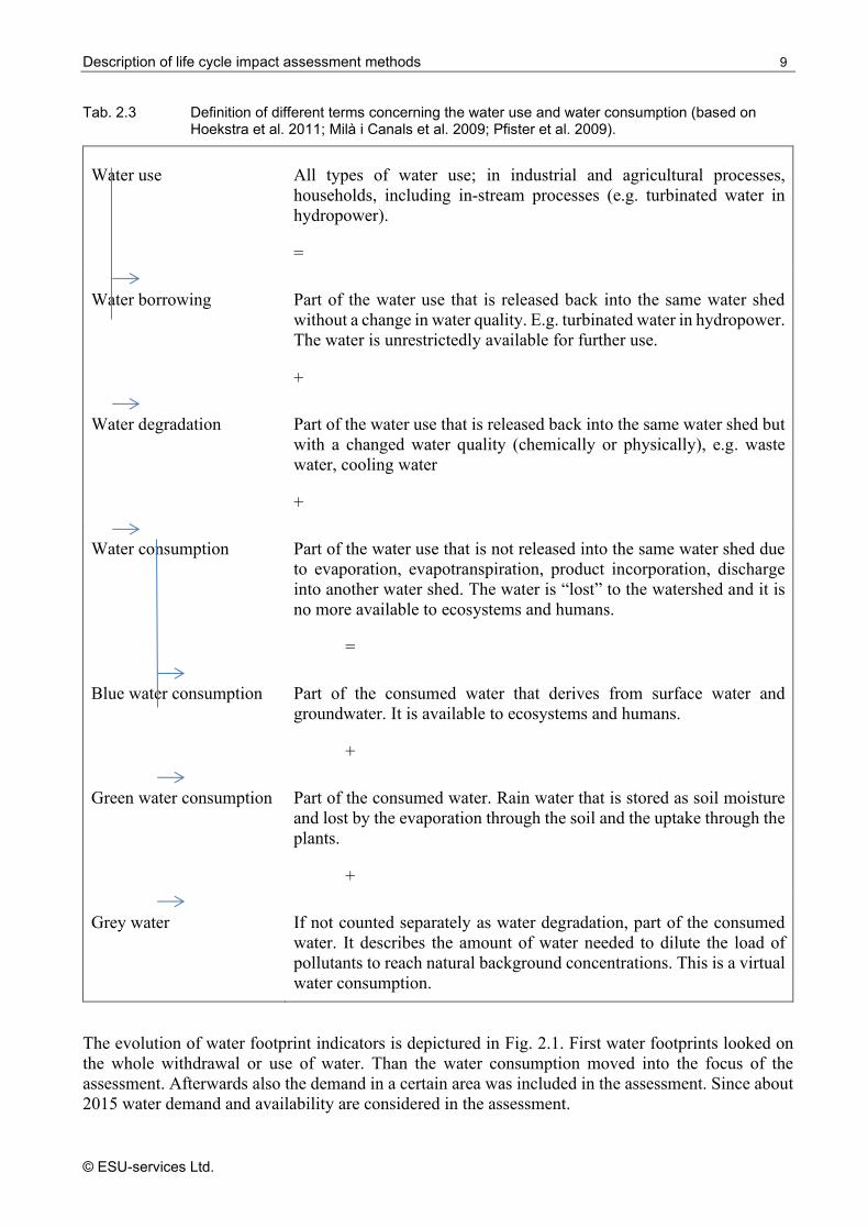
Tab. 2.3 Definition of different terms concerning the water use and water consumption (based on Hoekstra et al. 2011; Milà i Canals et al. 2009; Pfister et al. 2009).

Water use All types of water use; in industrial and agricultural processes,

households, including in-stream processes (e.g. turbinated water in

hydropower).

=

Water borrowing Part of the water use that is released back into the same water shed

without a change in water quality. E.g. turbinated water in hydropower.

The water is unrestrictedly available for further use.

+

Water degradation Part of the water use that is released back into the same water shed but

with a changed water quality (chemically or physically), e.g. waste

water, cooling water

+

Water consumption Part of the water use that is not released into the same water shed due

to evaporation, evapotranspiration, product incorporation, discharge

into another water shed. The water is “lost” to the watershed and it is

no more available to ecosystems and humans.

=

Blue water consumption Part of the consumed water that derives from surface water and

groundwater. It is available to ecosystems and humans.

+

Green water consumption Part of the consumed water. Rain water that is stored as soil moisture

and lost by the evaporation through the soil and the uptake through the

plants.

+

Grey water If not counted separately as water degradation, part of the consumed

water. It describes the amount of water needed to dilute the load of

pollutants to reach natural background concentrations. This is a virtual

water consumption.

The evolution of water footprint indicators is depictured in Fig. 2.1. First water footprints looked on

the whole withdrawal or use of water. Than the water consumption moved into the focus of the

assessment. Afterwards also the demand in a certain area was included in the assessment. Since about

2015 water demand and availability are considered in the assessment.



Fig. 2.1 Evolution of scarcity indicators modelled in LCA1

2.4.2 AWARE-method (2018)

The AWARE (Available WAter REmaining) is the outcome of a 2-year consensus building process

by “Water Use in Life Cycle Assessment” (WULCA), a working group of the UNEP-SETAC Life

Cycle Initiative. This group developed a water scarcity midpoint method for use in LCA and for water

scarcity footprint assessments. The AWARE method is endorsed by the Joint Research Centre and

will eventually become a part of ILCD recommendation.

The characterization model for water scarcity footprints is applied for assessing impacts of water

consumption. The method is based on the quantification of the relative available water remaining per

area once the demand of humans and aquatic ecosystems has been met. It assesses the potential of

water deprivation, to either humans or ecosystems, building on the assumption that the less water

remaining available per area, the more likely another user will be deprived (Núñez et al. 2016).

It is answering the question “What is the potential to deprive another user (human or ecosystem) when

consuming water in this area?” The resulting characterization factor (CF) ranges between 0.1 and 100

and can be used to calculate water scarcity footprints as defined in the ISO standard (Boulay et al.

2018). Importantly, the users looked at are both humans and ecosystems (see Fig. 2.2).

1 http://www.wulca-waterlca.org/aware.html

http://www.wulca-waterlca.org/aware.html



Fig. 2.2 Descriptive model of the AWARE indicator2

The characterisation factors are first calculated as the water Availability Minus the Demand (AMD)

of humans and aquatic ecosystems and is relative to the area (m3/m2/month). In a second step, the

value is normalized with the world average result (AMD = 0.0136 m3/m2/month) and inverted. The

characterisation factor than represents the relative value in comparison with the average m3 consumed

in the world (the world average is calculated as a consumption-weighted average). Once inverted,

1/AMD can be interpreted as a surface-time equivalent to generate unused water in this region. The

indicator is limited to a range from 0.1 to 100, with a value of 1 corresponding to the world average,

and a value of 10, for example, representing a region where there is 10 times less available water

remaining per area than the world average. The map below shows the factors at annual level per

watersheds (normal average over 12 months).

Fig. 2.3 Map of AWARE factors for non-agricultural activities (normal average over 12 months) Interpretation

– Spatio-temporal scale

The indicator was calculated at the sub-watershed level and monthly time-step, and then aggregated

in SimaPro to country and annual resolution. This aggregation can be done in diverse ways to better

represent an agricultural use or a domestic/industrial use, based on the time and region of water use.

Characterization factors for agricultural and non-agricultural use are provided in the method, as well

2 https://simapro.com/2017/whats-new-simapro-8-3/, 05.03.2018

https://simapro.com/2017/whats-new-simapro-8-3/



as default (“unknown”) ones if the activity is not known. The interpretation of results can be seen

relative to the world average.3

It must be noted that an aggregated value at country/annual level based on consumption:

• Does not represent the “average picture” of the country/year. It may completely exclude large

regions where no/very low consumption occur (i.e. deserts, most of Canada, etc.).

• Is strongly influenced by agricultural water use (in both “unknown” and “agri” values).

• Represents where/when water is most consumed: often in dryer months/regions.

For use with the ESU database (ESU 2020; Jungbluth et al. 2020), some special features must be taken

into account. The AWARE factors in SimaPro (for the ecoinvent v3 database) also evaluate the water

quantity for water turbines and cooling. However, the databases based on v2 do not include the

corresponding return flows into the catchment area. Therefore these contributions are ignored. This is

in line with the procedure used in FOEN studies (Jungbluth & Meili 2018).

2.4.3 Former assessment methods

Different LCIA methods are available for the assessment of water use and consumption (e.g. Milà i

Canals et al. 2009; Pfister et al. 2009 or Hoekstra et al. 2011). In this section we provide an overview

and we motivate the choice of the method applied in this study. Data availability is considered too.

The ReCiPe method (Goedkoop et al. 2009) quantifies the water use on a mid-point level but it is not

considered in the end-point indicators. The category of the water depletion (WD) includes the water

use from lakes, rivers, wells and unspecific natural origin.

The Water Footprint (Hoekstra et al. 2011) is a widely known and applied method to quantify the

water consumption. The Water Footprint quantifies the blue, green and grey water of the direct

(foreground system) and indirect (background system) water consumption. The water returned to the

same watershed is not considered whereas the inter-basin water transfer is defined as consumption.

The Water Footprint does not measure or asses the related environmental impacts of the water

consumption. The blue and green water consumption is defined by the crop water use (m3/ha) and the

yield. The grey water consumption is calculated from the chemical application rate to the field (kg/ha),

the leaching-run-of fraction as well as the maximum acceptable and the natural concentration for the

most important pollutant, i.e. the pollutant that yields the highest grey water volume. This approach

cannot be applied in a life cycle assessment because it requires unit process specific calculations

instead of generic characterisation factors.

The approach of Milà I Canals et al. (2009) focuses on two impact pathways of the freshwater

consumption: the freshwater ecosystem impact (FEI) and the freshwater depletion (FD). The FEI

describes the effects on the ecosystem quality due to changes in the freshwater availability and in the

water cycles as a result of land use changes. For the FEI, a water stress index (WSIMilà) for different

river basins is defined and used as mid-point characterisation factor. It is the ratio of the water

withdrawal to the water available for human use after subtracting the needed amount of water for

ecosystems (Smakhtin et al. 2004). The method of Milà I Canals et al. considers blue and indirectly

green water consumption. The blue water is differentiated between flow (rivers and lakes), fund

(aquifers) and stock (fossil).The discharge of used water to another watershed is not considered as

water consumption. Concerning the consumption of green water, Milà I Canals et al. (2009) argue that

it does not have a direct impact on the environment and as a consequence it should not be considered

3 It should be noted that a characterisation factor value of 1 is not equivalent to the factor for the average water

consumption in the world, i.e. the world average factor to use when the location is not known. This value is calculated as

the consumption-weighted average of the factors, which are based on 1/AMD and not AMD, hence the world

consumption-based average has a value of 43 for unknown use and 20 and 46 respectively for non-agricultural and

agricultural water consumption respectively. http://www.wulca-waterlca.org/aware.html, 05.03.2018.




in the LCIA. It is rather the change in land use that should be assessed as it affects the infiltration and

the evapotranspiration and consequently the availability of freshwater to other users. Following the

land occupation categories of ecoinvent, land use effects are quantified. This factor and the WSIMilà

result in the FEI. Seasonal fluctuations and regional differences along the river are not considered.

The reduced long-term availability of groundwater due to its use is described by the FD. The baseline

method for abiotic resources depletion in the CML 2001 guidelines (Guinée et al. 2001a) is adapted

for the development of characterisation factors for the FD. As the groundwater reserves are seldom

quantified this approach is characterised with high uncertainties.

In the approach of Pfister et al. (2009) mid-point and end-point characterisation factors are provided

for the assessment of the environmental impact of the water consumption. The method is adapted to

the Eco-indicator-99 impact assessment method (Goedkoop & Spriensma 2000b). The focus lies on

three areas of protection: human health, ecosystem quality and resources. The effects of water

consumption on human health is characterised by the lack of water for irrigation, which consequently

leads to malnutrition. The reduced availability of freshwater in ecosystems eventually leads to a

diminished vegetation and biodiversity; and consequently, to a reduced ecosystem quality. The

damages to resources described by Pfister et al. (2009) follow the concept of the abiotic resource

depletion applied in EI99 (Goedkoop & Spriensma 2000b), where the “surplus energy” (MJ) needed

to make the resource available in the future is used as indicator. In the context of water consumption,

the energy use for desalination of seawater might be applied as a worst-case assumption (maximum

estimation).

The approach of Pfister et al. (2009) considers only the consumption of blue water. It is defined as

water that is no longer available to the water shed. Green water is not included directly but it is

mentioned that with the lack of blue water the availability of green water might eventually be reduced

too. A water stress index (WSIPfister) relates the water consumption to the water scarcity and serves as

mid-point characterisation factor. The WSIPfister accounts for the spatial variability in precipitation as

well as the effects of strong regulations of flows. Even though the index is applicable to any spatial

scale, the authors recommend to assess the water consumption on the water shed level.

The eco-scarcity method (Frischknecht et al. 2009) defines the scarcity of freshwater according to

the water stress index of OECD (2004): Share of consumption to the available water resource

(precipitation + inflows – evaporation). Based on national levels of water consumption and the

acceptable water stress index defined by the OECD (2004), eco-factors are defined for the OECD-

countries, the average of the OECD-countries and for six different levels of water scarcity.

Furthermore, eco-factors are available on a watershed level4. The eco-factors are applicable to all types

of water uses or consumptions except for the in-stream water use in hydroelectric power plants. The

eco-factor can be applied on the (net) water withdrawal of drinking water supply, irrigation, industrial

processes (incl. cooling water), etc. If fossil (non-renewable) water is consumed, the eco-factors of the

most severe water stress category are to be applied. The water consumption is assessed on the midpoint

as well as on the endpoint level. The European research institute DG-JRC in Ispra recommends the

ecological scarcity approach for the assessment of water use and consumption as a mid-point indicators

in LCIA (DG-JRC IES 2011).

There are no requirements and guidelines for the assessment and reporting of water footprints yet

published by the International Organization for Standardization (ISO)5. As a basis for the

assessment of the methods presented and as a supporting information for the choice of one or more

methods, the latest working draft (ISO 14046.3, International Organization for Standardization (ISO)

2011) is summarised shortly: According to this ISO draft, not only the amount of water consumption

is to be considered but also the change in water quality. It is stated though that double-counting of the

change in water quality (e.g. in combination with other impact categories) shall be avoided. The form

4 http://www.esu-services.ch/projects/ubp06/google-layer/ 5 http://www.iso.org/iso/home.html



of water use considered is the water consumption according to the definition described above in Tab.

2.3. According to the ISO draft (2011), the applied assessment method should take into account the

change in water availability for humans and other species, the different water sources (e.g.

groundwater, surface water, sea water) as well as the quality of the water returned. The assessment

should furthermore include regional conditions. A multi impact categories approach should at least

differentiate between impacts on ecosystems, human health and on resources.

In Tab. 2.4 the main characteristics of the presented methods are summarized.

While the Water Footprint simply summarizes the water consumption and does not assess its

environmental impact, the other three specified methods include at least one characterisation step. The

Water Footprint may serve as a good guideline in the data collection but not as assessment method.

Pfister et al. (2011) as well as Frischknecht et al. (2009) have developed methods which assess the

impact of the consumption of water resources. Both methods offer a midpoint as well as an endpoint

indicator. While the assessment of the water use is part of the eco-scarcity method (Frischknecht et al.

2009), the method of Pfister et al. (2011) is easily combinable with the Eco-Indicator 99 (Goedkoop

& Spriensma 2000b). This allows for the comparison of products and services on an endpoint level.

This is not possible with the approach of Milà I Canals et al. (2009). Nevertheless, its consideration of

the land use change might be very interesting for certain specific questions and comparisons.

The impacts of water use and consumption of the product systems under study are consequently

assessed with the LCIA methods developed by Pfister et al. (2011) as well as the method proposed by

Frischknecht et al. (2009).



Tab. 2.4: Overview of different approaches to quantify and assess the impacts of water consumption.

Method Impact pathways Available data Required data/if specific calculations

are requested

Integration in existing LCI

/ LCIA

Indicator

Water Footprint

(Hoekstra et al.

2011)

- -Product water footprint (e.g. global ethanol

from sugarcane, maize and other crops)

-Water footprint of crop production at national,

sub-national and river basin level

-water footprint of rain-fed and irrigated

agriculture for maize, sugarcane and other

crops

-Crop water use (green and blue water)

-Chemical application rate

-Leaching-run-of fraction

-Max. acceptable concentration

-Natural concentration

-ecoinvent data (used in the

background system) are not

compatible.

-required data: blue and/or

green water consumption of

the foreground and

background system

Water consumption (m3)

Milà I Canals et al.

(Milà i Canals et

al. 2009)

-Freshwater

ecosystem impact

-Freshwater

depletion

-Water stress index (WSI) for the world’s

main river basins

-Land use effects

-Blue water consumption (crop evaporation

requirement, effective rainfall, irrigation)

-Land use occupation and transformation

processes

-Water resource (WR)

-Environmental water requirement (EWR)

-Evaporative and non-evaporative uses of

fossil water and aquifers

-Extraction rate of resource

-Regeneration rate of resource

-Ultimate reserve of resource

Water use impacts:

ecosystem-equivalent water

(m3)

Abiotic depletion potential

(kg Sb eq)

Enhanced Eco-

indicator 99

(Pfister et al.

2009)

-Human health

-Ecosystem quality

-Resources

WTA by WaterGAP2

Water stress index (WSI)

Damage to human health (DALY)

Ecosystem damage

Damage to resources (MJ)

LCA impact factors (EI99):Human health,

ecosystem quality, resources and aggregated

on watershed level

-Blue water consumed

-Freshwater withdrawals

-Hydrological availability

-more parameters if the mid-point

characterisation factors need to be

calculated

Characterisation by WSI

possible. Midpoint: Impact

on human health (DALY),

ecosystem quality

(PDF*m2a) and resources

(MJ surplus) due to water

consumption. Endpoint:

EI99HA points

(Can be integrated in the

Eco-indicator 99 method)

Ecological scarcity

method

(Frischknecht et

al. 2009a)

-Water scarcity,

proxy indicator for

impacts related to

water use or

consumption

Eco-factors 2006 based on the water stress

index (WSI) of all countries in the world, for

different scarcity situations and on watershed

level

-Blue water use or consumption

-National/regional level of water

consumption

-Available water resources (from FAO

CropWat database)

- ecoinvent data (used in the

background system) can

easily be integrated if water

use is assessed

- required data: total water

use or consumption of the

foreground system

Eco-points (UBP)

IMPACT World+ (2019)

© ESU-services Ltd. 16

3 IMPACT World+ (2019)

3.1 What is ImpactWorld+?

ImpactWorld+ is a Life Cycle Impact Assessment (LCIA) methodology published in 20196 that

extends beyond current regional modelling capabilities to a global level in order to consistently assess

regional life cycle emission inventories in the context of a global economy. It should serve both

industries and public administrations, through life cycle assessment (LCA) practitioners to support

the development of production and consumption policies and to improve the products and services

provided, while reducing environmental and health impacts.

3.2 How does ImpactWorld+ differ from other LCIA methods?

Current LCIA methods have some drawbacks (lack of regionalization for impacts, multiple sources

of uncertainty including geographical and temporal variability). The ImpactWorld+ LCIA

methodology aims for a better decision-making by increasing the discrimination power of LCA. It

leads to more precise and environmentally relevant LCA results by applying more scientifically

reliable and state of the art models. ImpactWorld+ integrates uncertainty related to characterization

factors and/or impact categories, it uses leading edge characterization modelling. It is also the first

global regionalized method, which allows assessing and discriminating a same emission occurring in

different geographical locations across the globe.

3.3 Features

With IMPACT World+, a midpoint-damage framework with four distinct complementary viewpoints

to present an LCIA profile: (1) midpoint impacts, (2) damage impacts, (3) damages on human health,

ecosystem quality, and resources & ecosystem service areas of protection, and (4) damages on water

and carbon areas of concerns, is proposed. Most of the regional impact categories have been spatially

resolved and all the long-term impact categories have been subdivided between shorter- term damages

(over the 100 years after the emission) and long-term damages.

The IMPACT World+ method integrates developments in the following categories, all structured

according to fate (or competition/scarcity), exposure, exposure response, and severity: (a)

Complementary to the global warming potential (GWP100), the IPCC Global Temperature Potentials

(GTP100) are used as a proxy for climate change long-term impacts at midpoint. At damage level,

shorter-term damages (over the first 100 years after emission) are also differentiated from long-term

damages. (b) Marine acidification impact is based on the same fate model as climate change,

combined with the H+ concentration affecting 50% of the exposed species. (c) For mineral resources

depletion impact, the material competition scarcity index is applied as a midpoint indicator. (d)

Terrestrial and freshwater acidification impact assessment combines, at a resolution of 2° × 2.5°

(latitude × longitude), global atmospheric source-deposition relationships with soil and water

ecosystems’ sensitivity. (e) Freshwater eutrophication impact is spatially assessed at a resolution grid

of 0.5° × 0.5°, based on a global hydrological dataset. (f) Ecotoxicity and human toxicity impact are

based on the parameterized version of USEtox for continents. The authors consider indoor emissions

and differentiate the impacts of metals and persistent organic pollutants for the first 100 years from

longer-term impacts. (g) Impacts on human health related to particulate matter formation are modeled

using the USEtox regional archetypes to calculate intake fractions and epidemiologically derived

exposure response factors. (h) Water consumption impacts are modeled using the consensus-based

scarcity indicator AWARE as a proxy midpoint, whereas damages account for competition and

6 https://link.springer.com/article/10.1007%2Fs11367-019-01583-0

https://link.springer.com/article/10.1007%2Fs11367-019-01583-0

PEF - European environmental footprint method (2018)


adaptation capacity. (i) Impacts on ecosystem quality from land transformation and occupation are

empirically characterized at the biome level.

The authors analyze the magnitude of global potential damages for each impact indicator, based on

an estimation of the total annual anthropogenic emissions and extractions at the global scale (i.e.,

Bdoing the LCA of the world^). Similarly with ReCiPe and IMPACT 2002+, IMPACT World+ finds

that (a) climate change and impacts of particulate matter formation have a dominant contribution to

global human health impacts whereas ionizing radiation, ozone layer depletion, and photochemical

oxidant formation have a low contribution and (b) climate change and land use have a dominant

contribution to global ecosystem quality impact. (c) New impact indicators introduced in IMPACT

World+ and not considered in ReCiPe or IMPACT 2002+, in particular water consumption impacts

on human health and the long-term impacts of marine acidification on ecosystem quality, are

significant contributors to the overall global potential damage.

According to the areas of concern version of IMPACT World+ applied to the total annual world

emissions and extractions, damages on the water area of concern, carbon area of concern, and the

remaining damages (not considered in those two areas of concern) are of the same order of magnitude,

highlighting the need to consider all the impact categories. The spatial variability of human health

impacts related to exposure to toxic substances and particulate matter is well reflected by using

outdoor rural, outdoor urban, and indoor environment archetypes. For Bhuman toxicity cancer^

impact of substances emitted to continental air, the variability between continents is of two orders of

magnitude, which is substantially lower than the 13 orders of magnitude total variability across

substances. For impacts of water consumption on human health, the spatial variability across

extraction locations is substantially higher than the variations between different water qualities. For

regionalized impact categories affecting ecosystem quality (acidification, eutrophication, and land

use), the characterization factors of half of the regions (25th to 75th percentiles) are within one to two

orders of magnitude and the 95th percentile within three to four orders of magnitude, which is higher

than the variability between substances, highlighting the relevance of regionalizing.

3.4 Conclusions

IMPACT World+ provides characterization factors within a consistent impact assessment framework

for all regionalized impacts at four complementary resolutions: global default, continental, country,

and native (i.e., original and non-aggregated) resolutions. IMPACT World+ enables the practitioner

to parsimoniously account for spatial variability and to identify the elementary flows to be

regionalized in priority to increase the discriminating power of LCA. IMPACT World+ does not

provide recommended weighting factors.

4 PEF - European environmental footprint method (2018) The EF method is the impact assessment method of the Environmental Footprint initiative. The

implementation is based on EF method 2.0.7 The approach is a further development of the ILCD

method (European Commission et al. 2011). It contains some updates and includes normalization and

weighting.

Sources:

• Characterization (Fazio et al. 2018)

• Normalization and weighting sets from Annex 2 of the Product Environmental Footprint Category

Rules Guidance.

7 http://eplca.jrc.ec.europa.eu/LCDN/developerEF.xhtml

http://eplca.jrc.ec.europa.eu/LCDN/developerEF.xhtml



• Normalization: World population used to calculate the NF per person: 6895889018 people;

Source: United Nations, Department of Economic and Social Affairs, Population Division (2011).

World Population Prospects: The 2010 Revision, DVD Edition – Extended Dataset (United

Nations publication, Sales No. E.11.XIII.7).

• Weighting: Sala S., Cerutti A.K., Pant R., Development of a weighting approach for the

Environmental Footprint (Sala et al. 2018).

4.1 Climate Change

Impact indicator: Global Warming Potential 100 years

Baseline model of the IPCC 2013 (IPCC 2013) and some additional factors calculated by the JRC.

4.2 Ozone depletion

Impact indicator: Ozone Depletion Potential (ODP) calculating the destructive effects on the

stratospheric ozone layer over a time horizon of 100 years.

4.3 Ionising radiation - human health

Impact indicator: Ionizing Radiation Potentials: Quantification of the impact of ionizing radiation on

the population, in comparison to Uranium 235.

4.4 Photochemical ozone formation - human health

Ozone and other reactive oxygen compounds are formed as secondary contaminants in the

troposphere (close to the ground). Ozone is formed by the oxidation of the primary contaminants

VOC (Volatile Organic Compounds) or CO (carbon monoxide) in the presence of NOx (nitrogen

oxides) under the influence of light.

Impact indicator: Photochemical ozone creation potential (POCP): Expression of the potential

contribution to photochemical ozone formation.

The method used includes spatial differentiation and is only valid for Europe. Considering a marginal

increase in ozone formation, the LOTOS-EUROS spatially differentiated model averages over 14000

grid cells to define European factors.

4.5 Respiratory inorganics

Impact indicator: Disease incidence due to kg of PM2.5 emitted

The indicator is calculated applying the average slope between the Emission Response Function

(ERF) working point and the theoretical minimum-risk level. Exposure model based on archetypes

that include urban environments, rural environments, and indoor environments within urban and rural

areas.

4.6 Non-cancer human health effects

Impact indicator: Comparative Toxic Unit for human (CTUh) expressing the estimated increase in

morbidity in the total human population per unit mass of a chemical emitted (cases per kilogramme).

USEtox consensus model (multimedia model). No spatial differentiation beyond continent and world

compartments. Specific groups of chemicals require further works (cf. details in other sections).



4.7 Cancer human health effects

Impact indicator: Comparative Toxic Unit for human (CTUh) expressing the estimated increase in

morbidity in the total human population per unit mass of a chemical emitted (cases per kilogramme).


compartments. Specific groups of chemicals require further works (cf. details in other sections).

4.8 Acidification terrestrial and freshwater

Impact indicator: Accumulated Exceedance (AE) characterizing the change in critical load

exceedance of the sensitive area in terrestrial and main freshwater ecosystems, to which acidifying

substances deposit.

4.9 Eutrophication freshwater

Impact indicator: Phosphorus equivalents: Expression of the degree to which the emitted nutrients

reaches the freshwater end compartment (phosphorus considered as limiting factor in freshwater).

European validity. Averaged characterization factors from country dependent characterization

factors.

4.10 Eutrophication marine

Impact indicator: Nitrogen equivalents: Expression of the degree to which the emitted nutrients

reaches the marine end compartment (nitrogen considered as limiting factor in marine water).

4.11 Eutrophication terrestrial

Impact indicator: Accumulated Exceedance (AE) characterizing the change in critical load

exceedance of the sensitive area, to which eutrophying substances deposit.

4.12 Ecotoxicity freshwater

Impact indicator: Comparative Toxic Unit for ecosystems (CTUe) expressing an estimate of the

potentially affected fraction of species (PAF) integrated over time and volume per unit mass of a

chemical emitted (PAF m3 year/kg).


compartments. Specific groups of chemicals requires further works (cf. details in other sections).

4.13 Land Use

Impact indicator: Soil quality index

CFs set was re-Calculated by JRC starting from LANCA® v 2.2 as baseline model. Out of 5 original

indicators only 4 have been included in the aggregation (physico-chemical filtration was excluded

due to the high correlation with the mechanical filtration).

4.14 Water scarcity

Impact indicator: m3 water eq. deprived.

Relative Available WAter REmaining (AWARE) per area in a watershed, after the demand of

humans and aquatic ecosystems has been met (Boulay et al. 2018).

Environmental product declaration (Environdec) (2018)


4.15 Resource use, energy carriers

Impact indicator: Abiotic resource depletion fossil fuels (ADP-fossil); based on lower heating value

ADP for energy carriers, based on van Oers et al. 2002 as implemented in CML, v. 4.8 (2016).

Depletion model based on use-to-availability ratio. Full substitution among fossil energy carriers is

assumed.

4.16 Resource use, mineral and metals

Impact indicator: Abiotic resource depletion (ADP ultimate reserve)

ADP for mineral and metal resources, based on van Oers et al. 2002 as implemented in CML, v. 4.8

(2016). Depletion model based on use-to-availability ratio. Full substitution among fossil energy

carriers is assumed.

5 Environmental product declaration (Environdec) (2018) This is a list of characterisation models and factors to use for the default environmental impact

categories.8 This recommendation is updated on a regular basis. It is based on the latest developments

in LCA methodology and ensuring the market stability of EPDs. The latest update to the

recommendations was made 2018-05-30 (Photo-oxidation Formation Potential, short: POFP) and

2018-06-08 (Water Scarcity Footprint).

5.1 Default indicators

The characterisation models and factors to use for the default impact categories are available in the

table below.

8 https://www.environdec.com/Creating-EPDs/Steps-to-create-an-EPD/Perform-LCA-study/Characterisation-factors-

for-default-impact-assessment-categories/

https://www.environdec.com/Creating-EPDs/Steps-to-create-an-EPD/Perform-LCA-study/Characterisation-factors-for-default-impact-assessment-categories/

https://www.environdec.com/Creating-EPDs/Steps-to-create-an-EPD/Perform-LCA-study/Characterisation-factors-for-default-impact-assessment-categories/

Environmental product declaration (Environdec) (2018)


Tab. 5.1 Default environmental impact categories

Impact category (Unit) Characterisation factors Original

reference(s) Examples

Global warming potential (kg

CO2 eq.) in SimaPro 'Global

warming (GWP100a)'

GWP100, CML 2001 baseline

Version: January 2016. IIPCC 2013

1 kg carbon dioxide = 1 kg

CO2 eq.

1 kg methane = 28* kg CO2 eq.

1 kg dinitrogen oxide = 265 kg

CO2 eq.

Acidification potential (kg

SO2 eq.) in SimaPro

'Acidification (fate not incl.)'

AP, CML 2001 non-

baseline (fate not included),

Version: January 2016.

Please notice the use of non-baseline

characterisation factors for acidification

potential.

Hauschild &

Wenzel 1997

1 kg ammonia = 1.88 kg

SO2 eq.

1 kg nitrogen dioxide = 0.7 kg

SO2 eq.

1 kg sulphur dioxide = 1 kg

SO2 eq.

Eutrophication potential (kg

PO43- eq.) in SimaPro

'Eutrophication'

EP, CML 2001 baseline (fate not

included), Version: January

2016.

Heijungs et al.

1992

1 kg phosphate = 1 kg

PO43- eq.

1 kg ammonia = 0.35 kg kg

PO43- eq.

1 kg COD (to freshwater) =

0.022 kg kg PO43- eq.

Photochemical oxidant

formation potential (kg

NMVOC eq.) in SimaPro

'Photochemical oxidation'

POFP, LOTOS-EUROS as

applied in ReCiPe 2008

Goedkoop et al.

2009; Van Zelm

et al. 2008

1 kg carbon monoxide = 0.046

kg NMVOC eq.

1 kg nitrogen oxides = 1 kg

NMVOC eq.

Abiotic depletion potential –

Elements (kg Sb eq.) in

SimaPro 'Abiotic depletion,

elements'

ADPelements, CML 2001,

baseline

van Oers et al.

2002

1 kg antimony = 1 kg Sb eq.

1 kg aluminium = 1.09 * 10^-9

Sb eq.

Abiotic depletion potential –

Fossil fuels (MJ, net calorific

value) in SimaPro 'Abiotic

depletion, fossil fuels'

ADPfossil fuels, CML 2001,

baseline

van Oers et al.

2002

1 kg coal hard = 27.91 MJ

1 kg coal soft, lignite = 13.96

MJ

Water Scarcity Footprint (WSF)

(m3 H2O eq) in SimaPro 'Water

scarcity'

AWARE Method: WULCA

Recommendations on

characterization model for WSF

2015, 2017.

Boulay et al. 2018

Example: 582 m3 H2O

consumed per ton of grapes

produced in Mendoza,

Argentina :

WSF = 582 m3H2O x 54.15

(CFAgriAWARE100) = 31,518

m3eq/ton grape

For construction product EPDs compliant with EN 15804, Table 3 in EN 15804 (“Parameters

describing environmental impacts”) shall be applied in the PCR instead of the indicators listed above.

Characterisation factors are available in Annex C of the standard.

The source and version of the characterisation models and the factors used shall be reported in the

EPD. Alternative regional life cycle impact assessment methods and characterisation factors are

allowed to be calculated and displayed in addition to the default list. If so, the EPD shall contain an

explanation of the difference between the different sets of indicators, as they may appear to the reader

to display duplicate information.

https://www.universiteitleiden.nl/en/research/research-output/science/cml-ia-characterisation-factors#downloads












Swiss environmental footprint indicators (2018)


5.2 Use of ressources

Tab. 5.2 Indicators for the use of ressources

5.3 Waste production and output flows

Tab. 5.3 Indicators for waste production and output flows

5.4 Additional indicators

To better characterise the environmental performance of a product category, the PCR shall indicate

the mandatory or voluntary use of other indicators of potential impacts. All environmentally-relevant

indicators for the product category shall be included. Examples of such environmental impact

categories to include in the PCR are:

• emission of ozone-depleting gases, in SimaPro 'Ozone layer depletion (ODP) (optional)'

• land use and land use change.

6 Swiss environmental footprint indicators (2018) Set of LCIA indicators applied by the FOEN (Frischknecht et al. 2018). Overview:

• Overall environmental footprint. Ecological scarcity method 2013 (Frischknecht et al. 2013)

• Greenhouse gas footprint (Solomon et al. 2007)

• Biodiversity footprint (Chaudhary et al. 2015; Chaudhary et al. 2016)

• Eutrophication footprint (Marine eutrophication, Goedkoop et al. 2009)

UNIT

Use as energy carrier PERE MJ, net calorif ic value

Used as raw materials PERM MJ, net calorif ic value

Primary energy resources – Renew able TOTAL PERT MJ, net calorif ic value

Use as energy carrier PENRE MJ, net calorif ic value

Used as raw materials PENRM MJ, net calorif ic value

Primary energy resources – Non-renew able TOTAL PENRT MJ, net calorif ic value

SM kg

RSF MJ, net calorif ic value

NRSF MJ, net calorif ic value

FW m3

Use of resources

PARAMETER

Secondary material

Renew able secondary fuels

Non-renew able secondary fuels

Net use of fresh w ater

Waste production

PARAMETER UNIT

Hazardous w aste disposed HWD kg

Non-hazardous w aste disposed NHWD kg

Radioactive w aste disposed RWD kg

Output flows

PARAMETER UNIT

Components for reuse CRU kg

Material for recycling MFR kg

Materials for energy recovery MER kg

Exported energy, electricity EE MJ

Exported energy, thermal EE MJ

Swiss environmental footprint indicators (2018)


• Air pollution footprint (particulate matter, Goedkoop et al. 2009)

• Water footprint (Kounina et al. 2013)

• Material footprint (Ores, minerals, fossil energy, (woody) biomass) (Schoer et al. 2012).

Overall environmental footprint according to the Ecological scarcity method 2013 (Frischknecht et

al. 2013).

Climate change (greenhouse gas footprint): The climate impact of greenhouse gases is expressed in

terms of global warming potential (GWP) according to the 4th Assessment Report of the

Intergovernmental Panel on Climate Change (CO2 equivalents according to IPCC 2007). The

additional heating effects of stratospheric emissions from aircraft are considered with a small factor.

The calculation of the corresponding characterization factors is described in the technical report

(Frischknecht et al. 2018). These emissions are also covered in the overall environmental footprint.

Loss of biodiversity through land occupation (biodiversity footprint): Land occupation has a major

impact on biodiversity and species loss. The indicator for the species loss potential (Chaudhary et al.

2016) quantifies the potential damage of land use in relation to biodiversity. The indicator quantifies

the loss of species in amphibians, reptiles, birds, mammals and plants by using an area as farmland,

permanent crop, pasture, intensively used forest, extensively used forest or settlement area. The

indicator weighted endemic species higher than species that are common. The loss of species is

determined in relation to the biodiversity of the natural state of the area in the region concerned. This

indicator was recommended by the UNEP SETAC Life Cycle Initiative as currently the best available

indicator for a transitional period ("interim recommendation", Chaudhary et al. 2015; Chaudhary et

al. 2016; Frischknecht & Jolliet 2017). Impacts on biodiversity are covered also in the overall

environmental footprint with several different factors (land occupation, water use, eutrophication,

pesticides, acidification, etc.).

Overfertilization (eutrophication footprint): The introduction of nitrogen into the environment

causes a wide range of problems. The most obvious of these is marine eutrophication

("overfertilization"): This indicator quantifies the amount of nitrogen that potentially enters the

oceans via the emission of nitrogen compounds into water, air and soil and contributes to

overfertilization there (Goedkoop et al. 2009). The quantities of nitrogen are considered according to

their marine eutrophication potential (kg N equivalents). These emissions are also covered in the

overall environmental footprint.

Particulate matter (air pollution footprint): The extent of air pollution has a major influence on the

health and thus the well-being of the population. Air pollution is described with primary and

secondary particles and the associated effects on human health, such as respiratory diseases

(Goedkoop et al. 2009). The emissions of the fine dust precursors NOX, SO2 and NH3 are added to

the direct emissions of fine dust according to their potential to form fine dust (kg PM10 equivalents).

These emissions are also covered in the overall environmental footprint.

Water use (water footprint): Describes how much Switzerland uses the global resource (fresh) water,

considering the water shortage in the production regions. This is illustrated by the water scarcity

indicator AWARE recommended by the UNEP SETAC Life Cycle Initiative (Boulay et al. 2018).

Specifications: consuming water use, non-specific activity. Within some background databases water

flows are only partly regionalized. These resource uses are also covered in the overall environmental

footprint.

Raw materials (material footprint, RMC): The material footprint quantifies the consumption of raw

materials at home and abroad caused by a country's domestic final demand. The Swiss material

footprint is collected by the FSO according to the method of the Statistical Office of the European

Union (Eurostat) and divided into the categories ores, minerals, fossil fuels and biomass (BFS 2015).

In this study, the material footprint is modelled with the data used here to determine the influence of

Environmental impacts according to ReCiPe (2016)


method and data basis on the results. For the quantification of the material footprint, the total amount

of materials required for the manufacture of a product is considered, not just the product itself. Each

raw material extraction is multiplied accordingly by one raw material equivalent (RÄ, quantity ore

per kg metal, 95.8 kg ore per kg copper). The RÄ factors for ores are based on data from Schoer et al

(2012). Only woody biomass is considered with the implementation of this method provided by

FOEN and the KBOB database. No elementary flows concerning the production of agricultural

biomass are recorded in the KBOB database that could be used with the factors provided for fish,

fodder, etc. No extensions have been made to the background database for this indicator. These

resource uses are also covered in the overall environmental footprint.

7 Environmental impacts according to ReCiPe (2016)

7.1 ReCiPe 2016

The authors of the updated ReCiPe 2016 (Huijbregts et al. 2017) implemented human health,

ecosystem quality and resource scarcity as three areas of protection. Endpoint characterisation factors,

directly related to the areas of protection, were derived from midpoint characterisation factors with a

constant mid-to-endpoint factor per impact category. The authors included 18 midpoint impact

categories.

The update of ReCiPe provides characterisation factors that are representative for the global scale

instead of the European scale, while maintaining the possibility for a number of impact categories to

implement characterisation factors at a country and continental scale. The authors also expanded the

number of environmental interventions and added impacts of water use on human health, impacts of

water use and climate change on freshwater ecosystems and impacts of water use and tropospheric

ozone formation on terrestrial ecosystems as novel damage pathways. Although significant effort has

been put into the update of ReCiPe, there is still major improvement potential in the way impact

pathways are modelled. Further improvements relate to a regionalisation of more impact categories,

moving from local to global species extinction and adding more impact pathways.

No single score weighting is proposed anymore for the updated version, but the weighting scheme

proposed for the previous version still might be applied.

7.2 ReCiPe 2008 (partly outdated)

The ReCiPe 2008 method (Goedkoop et al. 2009) was developed by the Dutch National Institute for

Public Health and the Environment (RIVM), the Radboud University, the Dutch Institute of

Environmental Sciences (CML) at Leiden University and PRé Consultants.

The method determines environmental indicators at midpoint and endpoint level. Analyses on both

levels are possible. The following eighteen ReCiPe midpoint indicators are calculated (the reference

substance is indicated in brackets):

• Climate change (kg CO2 eq.)

• Ozone depletion (ODP) (kg CFC-11 eq.)

• Terrestrial acidification (kg SO2 eq.)

• Freshwater eutrophication (kg P eq.)

• Marine eutrophication (kg P eq.)

• Human toxicity (kg 1,4-DB eq.)

• Photochemical oxidation (kg NMVOC eq.)

• Particulate matter formation (kg PM10 eq.)

• Terrestrial ecotoxicity (kg 1,4-DB eq.)

Swiss Ecological Scarcity Method 2013 (eco-points 2013)


• Freshwater ecotoxicity (kg 1,4-DB eq.)

• Marine ecotoxicity (kg 1,4-DB eq.)

• Ionising radiation (kg U235 eq.)

• Agricultural land occupation (m2*yr eq.)

• Urban land occupation (m2*yr eq.)

• Natural land transformation (m2 eq.)

• Water depletion (m3 eq.)

• Mineral resource depletion (kg Fe eq.)

• Fossil resource depletion (kg oil eq.)

The midpoint indicators are aggregated to three endpoint indicators:

• Damage to Human health (Disability-adjusted loss of life years)

• Damage to ecosystems (Loss of species during a year)

• Damage to resource availability (Increased cost)

The damages to these three safeguard subjects are weighted and aggregated to one single score. Three

different perspectives were developed to represent different perceptions of the world with regard to

time preference, uncertainty or local preference (hierarchist, individualist and egalitarian). The

hierarchist perspective is the most balanced type (balance between future and present impacts,

between risks and benefits and between his or her neighbourhood and the world).

8 Swiss Ecological Scarcity Method 2013 (eco-points 2013) The ecological scarcity method (Frischknecht et al. 2013) evaluates the inventory results on a distance

to target principle. The calculation of the eco-factors is based on one hand on the actual emissions

(actual flow) and on the other hand on Swiss environmental policy and legislation (critical flow).

These goals are:

• Ideally mandatory or at least defined as goals by the competent authorities,

• formulated by a democratic or legitimised authority, and

• preferably aligned with sustainability.

The weighting is based on the goals of the Swiss environmental policy; global and local impact

categories are translated to Swiss conditions, i.e. normalised. The method is applicable to other

regions as well. Eco-factors were also developed for the Netherlands, Norway, Sweden (Nordic

Council of Ministers 1995, Tab. A22 / A23), Belgium (SGP 1994), Germany (Ahbe et al. 2014) and

Japan (Miyazaki et al. 2004). The ecological scarcity method allows for an optimisation within the

framework of a country’s environmental goals.

The environmental and political relevance is essential for the choice of substances. The environmental

policy does by far not define goals for all substances. Thus, the list of eco-factors is limited. This

particularly applies to substances with low or unknown environmental relevance in Switzerland and

Europe (e.g. sulphate emissions in water bodies).

The Method of ecological scarcity allows the weighting of the resource withdrawals and pollutant

emissions recorded and calculated in a Life Cycle Inventory. The basic principles of the method were

first developed in 1978 (Müller-Wenk 1978). The first update took place in 1998 (Brand et al. 1998).



Another update took place between 2005 and 2008 (Frischknecht et al. 2008). The most recent version

was published in 2013 (Frischknecht et al. 2013).

The method of ecological scarcity is based on the "distance-to-target" principle. It uses the total

current fluxes of an environmental impact (e.g. nitrogen oxides) of a country on the one hand and the

fluxes of the same environmental impact that are considered maximum permissible (critical) within

the framework of the environmental policy objectives of the respective country on the other. Both

critical and current fluxes are defined in relation to Swiss conditions.

Fig. 8.1 shows a simplified procedure for this assessment method. This shows that the classification

and characterisation steps are only carried out for part of the environmental problems. Otherwise, the

environmental impacts (emissions and resource consumption) and waste quantities from the Life

Cycle Inventory are weighted directly.

Fig. 8.1 Schematic illustration of the method of ecological scarcity 2013 (Frischknecht et al. 2013)

The evaluation is carried out using ecofactors which are defined as follows:

Ecofactor = 𝐾⏟characterization(optional)

⋅1⋅UBP

𝐹𝑛⏟normalization

⋅ (𝐹

𝐹𝑘)2

⏟ weighting

⋅ 𝑐⏟constant

(8.1)

with: K = Characterisation factor of a pollutant or resource

Flow = Cargo of a pollutant, consumption quantity of a resource or quantity of a characterised environmental

impact

Fn = Normalisation flow: Current annual flow, relative to Switzerland

F = Current flow: Current annual flow, related to the reference area.



Fk = Critical flow: Critical annual flow relative to the reference area.

c = Constant (1012/a)

UBP = Environmental Impact Point: Unit of the evaluated result.

Factor c is identical for all ecofactors and serves to improve the manageability of the numbers. The

first factor is used for characterisation and is applied to pollutants (or resources) that have the same

environmental impact (e.g. climate change). The characterisation factor is optional in this method,

i.e. not all pollutants are characterised in this method. The second term is used for

standardization/normalization and contains the denominator of today's Swiss flux. This is either given

in characterised form (e.g. tonnes of CO2 equivalents per year) if a characterisation factor is applied

to the relevant pollutant, or in its original form (e.g. tonnes of PM10 per year) if the pollutant has no

characterisation factor. The third term contains the weighting step. Here the current emissions on the

one hand and the targeted emission goal on the other hand are put into proportion and squared.

The ratio of current to critical flow is taken into account as a square. This has the effect that strong

overruns of the target value (critical flow) are weighted disproportionately and strong underruns are

weighted disproportionately, i.e. an additional emission is weighted more strongly the higher the

pollution situation already is.

Thousands of environmental impact points (1000 UBP) correspond to the reference values shown in

Tab. 8.1.

Tab. 8.1 Reference values for products and services causing 1000 environmental impact points

2114 litres of tapwater from Switzerland

4.25 centimeters road, used for one year

2.17 kilograms of fossil CO2, directly emitted

0.08 kilograms of fossil methane, directly emitted

0.071 grams copper input into agricultural soil

1.24 litres crude oil produced, with transport to the refinery

33 kilograms of gravel mining

3.33 grams pesticide application in agriculture

2.1% of a person's private daily consumption in Switzerland, 2018

4.5 km transport of one person by plane

4.5 km transport of one person by car (occupancy 1.6 persons)

96 km transport of one person by bicycle

6% of a vegetarian menu with 4 courses

4% of a meaty 3-course menu

7% of the daily food consumption of a person in Switzerland, 2018

38 plastic carrier bags (production, distribution and disposal)

0.08 cotton T-Shirts

0.23% of the production of a laptop

31% of daily consumption for hobbies/leisure activities in Switzerland, 2018

63% of daily consumption of furniture and household appliances in Switzerland, 2018

ILCD recommended life cycle impact assessment methods (2010, outdated)


9 ILCD recommended life cycle impact assessment methods (2010, outdated)

9.1 Overview

The International Reference Life Cycle Data System (ILCD) recommends life cycle impact

assessment methods in the ILCD Handbook (European Commission et al. 2010). The methods at the

midpoint9 level are chosen. The methods describe potential and not measured effects related to

different environmental problems. They are listed in Tab. 9.1.

Some of these indicators might be more reliable than others for the available data and the questions

for this LCA.

9 Midpoint level means that environmental impacts are only summarized at the impact category level (i.e. climate

change, water use). Endpoint values summarize these results from the impact category further, i.e. to one single

value.



Tab. 9.1 Midpoint impact categories of the ILCD recommended LCIA

Impact category Impact assessment model Indicator unit Source

Climate change The Global Warming Potential (GWP) calculates the radiative forcing over a 100 year time

horizon. It assesses the potential impact of different gaseous emissions on climate change.

kg CO2 eq IPCC 2007 (International

Panel on Climate Change)

Ozone depletion The Ozone Depletion Potential (ODP) calculates the destructive effects on the stratospheric

ozone layer over a time horizon of 100 years. The stratospheric ozone layer reduces the

amount of UV-radiation that reaches the ground and which can cause damages for humans,

animals, plants and materials.

kg CFC-11

eq

WMO 1999 (World

Meteorological Organization)

Human toxicity,

non-cancer effects,

cancer effects

The unit “CTUh” (Comparative Toxic Unit for Humans) expresses the estimated increase in

morbidity in the total human population due to different types of emissions entering into the

environment. The calculation is based on USEtox, which is a model that describes chemical

fate, exposure, effect and optionally severity of emissions.

CTUh Rosenbaum et al. 2008

Particulate matter This category estimates the potential effect of fine dust emissions on human health:

Quantification of the impact of premature death or disability that particulates/respiratory

inorganics have on the population. It includes the assessment of primary (PM10 and PM2.5)

and secondary PM (incl. creation of secondary PM due to SOx, NOx and NH3 emissions)

and CO.

kg PM2.5 eq Humbert 2009 based on Rabl

& Spadaro 2004 and Greco et

al. 2007

Ionizing radiation This category estimates the effect of radioactive emissions on human health. Most radiation

stems from normal operation of nuclear power plants including the nuclear fuel production

and treatment of radioactive wastes (accidents are not included). Quantification of the impact

of ionizing radiation on the population is made with reference to Uranium 235.

kBq U235 eq

(to air)

Dreicer et al. 1995

Photochemical ozone

formation

This category calculates the effect of summer smog on human health.

Expression of the potential contribution to photochemical ozone formation close to the

ground. The method evaluates impacts on human health from ozone and other reactive

oxygen compounds (LOTOS-EUROS model) developed in the lower atmosphere due to

emissions e.g. of nitrogen dioxides.

kg NMVOC

eq

Van Zelm et al. 2008 as

appled in ReCiPe

Acidification This impact category describes potential impacts on soil and freshwater that becomes more

acid due to the deposition of certain pollutants from air:

The “Accumulated Exceedance” model characterizes the change in critical load exceedance

of the sensitive area in terrestrial and main freshwater ecosystems, to which acidifying

substances deposit.

molc H+ eq Posch et al. 2008

Seppälä et al. 2006

Terrestrial eutrophication Eutrophication means that too much nutrients reach ecosystems and harm the plants and

animals living in sensitive systems:

The “Accumulated Exceedance” model characterizes the change in critical load exceedance

of the sensitive terrestrial area, to which eutrophying substances (“excess nutrients”) deposit.

It is European-country dependent which is not considered with the LCI data used in this

study.

molc N eq Posch et al. 2008

Seppälä et al. 2006



Impact category Impact assessment model Indicator unit Source

Freshwater

eutrophication

Expression of the degree to which the nutrients emitted in Europe reach the freshwater and

lead to the problem of eutrophication. Only phosphorus emissions are evaluated since it is

considered as the limiting factor in freshwater. EUTREND model used to model atmospheric

emissions.

kg P eq Struijs et al. 2009 as

implemented in ReCiPe

Marine eutrophication Expression of the degree to which nutrients emitted in Europe reach the oceans and lead to

eutrophication. Only nitrogen emissions evaluated since it is considered as the limiting factor

in marine water. EUTREND model used to model atmospheric emissions.

kg N eq Struijs et al. 2009 as

implemented in ReCiPe

Freshwater ecotoxicity Measurement of environmental toxicity in freshwater due to emissions: The unit “CTUe”

(Comparative Toxic Unit for ecosystems) is an expression of an estimate of the potentially

affected fraction of species (PAF) integrated over time and volume per unit mass of a

chemical emitted (PAF m3 year/kg). Specific groups of chemicals require further works.

(USEtox model)

CTUe Rosenbaum et al. 2008

Land use Land use generally refers to the amount and quality deficit of land occupied or transformed.

This model is based on changes in Soil Organic Matter (SOM) due to different categories of

land use. SOM is a keystone soil quality indicator and influences properties like buffer

capacity, soil structure and fertility. Biodiversity impacts are not covered in this method.10

kg C deficit Mila i Canals et al. 2007

Water depletion Assessment of the water use related to local scarcity of water in different countries. (Swiss

Ecoscarcity model)

m3 water eq Frischknecht et al. 2008

Abiotic resource

depletion

The model covers mineral, fossil & renewable resource depletion. The model takes both the

annual production as well as the availability of the resource into account. (CML 2002 model)

kg antimony

(Sb) eq

van Oers et al. 2002

10 The LCIA method in SimaPro has assigned characterisation factors for elementary flows of land use in the ocean „benthos“. These factors have been removed after consulting the

authors of the method as they are not meaningful.



9.2 Long-term emissions

Some indicators are strongly dependent on long-term emissions. Such long-term emissions can only

be modelled in a quite unreliable way. Some databases such as ecoinvent investigate long-term

emissions of heavy metals and other pollutants (Frischknecht et al. 2007a). These emissions can take

place in a time frame of 100 to 60’000 years from now. They mainly stem from waste disposal in

landfills and deposits made during mining of metals.

If these long-term-emissions are included in the LCIA they can make up a considerable amount of

the total impacts in the ILCD impact categories. The analysis of e.g. heating options shows that in

five categories, a considerable part of total impacts solely stems from the long-term emissions if they

are included in the LCI:

• Human toxicity, non-cancer effects: 50 to 80%

• Human toxicity, cancer effects: 4 to 80%

• Ionizing radiation HH: around 70% for all datasets

• Freshwater eutrophication: 30 to 90%

• Freshwater ecotoxicity: 40 to almost 100%

If long-term emissions are included in the assessment, background data on e.g. machinery become

very relevant, but it is nearly impossible to check the appropriateness of this data.

An extensive discussion about the pros and cons of including long-term emissions in LCIA can be

found in the Ecoinvent report on LCIA methods (Frischknecht et al. 2007b).

ESU-services recommends excluding long-term emissions in the life cycle impact assessment

because of the high uncertainties involved. This is also in line with internal findings of the PEF studies

unfortunately not yet published.

9.3 Abiotic resource depletion

This impact category indicator assesses extraction of metals, minerals and fossil fuels. The Abiotic

Depletion Factor (ADF) is determined for each of these extraction materials and related to the scarcity

of antimony (Unit: kg antimony equivalents/kg extraction) based on concentration reserves and rate

of deaccumulation. By including the annual production, the current importance of a give resource is

also reflected. The annual production of the resource (the extraction rate) is divided by the reserves

squared, and the result divided by the same ratio for the reference resource, antimony. “The CML

method is recommended in the ILCD framework since it captures scarcity by including extraction as

well as reserves of a given resource. Characterization factors are given for metals, fossil fuels and, in

the case of reserve base and economic reserves, mineral compounds

The scarcity of resources is determined based on the 'Reserve base'. It refers to identified resources

that meet specified minimum physical and chemical criteria related to current mining practice.

Therefore, it may contain those parts of the resources that have a reasonable potential for becoming

economically available within planning horizons beyond those that assume proven technology and

current economics.

9.4 Ecotoxicity freshwater

The impact category ecotoxicity freshwater assesses the heavy metals and pesticides. The

characterization factor for the heavy metals are classified as “uncertain” while the ones for the

pesticides are “recommended”. It would be possible to separate the assessment of the heavy metals

to better interpret the impact assessment of the pesticides.

Impact 2002+ (outdated)


10 Impact 2002+ (outdated)

10.1 Introduction

IMPACT 2002+ is a combination of four methods: IMPACT 2002 (Pennington et al. 2005), Eco-

indicator 99 (Goedkoop and Spriensma. 2000, 2nd version, Egalitarian Factors), CML (Guinée et al.

2002) and IPCC.

Contact info: http://www.impactmodeling.org

The IMPACT 2002+ method was largely based on Eco-indicator 99. Compared to eco-indicator 99

the following changes were implemented:

• IMPACT 2002 factors replace Eco-indicator's Human Health carcinogenic and non-carcinogenic

factors and for Aquatic and Terrestrial ecotoxicity factors.

• CML factors were used for Aquatic acidification and Aquatic eutrophication. The Aquatic

eutrophication CF implemented in this method are those for a P-limited watershed.

• Climate change was redefined and separated from Human Health impacts and added as a separate

damage category. The characterisation factors of IPPC 2001 500a were used for this impact

category.

• For fossil fuel depletion the Energy content was used instead of the surplus energy needed for

extraction. In the Resource depletion category however, results for mineral extraction and fossil

fuel depletion were added together even though fossil energy content and surplus energy for

minerals represent different concepts.

• The Eco-indicator 99 factors for Respiratory effects, Ionizing radiations, Land use and Mineral

extraction remained unchanged.

10.2 Midpoint indicators

The respective midpoint units are the following:

• kg chloroethylene equivalents into air (written “kg C2H3Cl eq”) for Carcinogens and Non-

carcinogens,

• kg PM2.5 equivalents into air (written “kg PM2.5 eq”) for Respiratory inorganics,

• Bq C-14 equivalents into air (written “Bq C-14 eq”) for Ionizing radiation,

• kg CFC-11 equivalents into air (written “kg CFC-11 eq”) for Ozone layer depletion,

• kg ethylene equivalents into air (written “kg C2H4 eq”) for Respiratory organics,

• kg triethylene glycol equivalents into water (written “kg TEG water”) for Aquatic ecotoxicity,

• kg triethylene glycol equivalents into soil (written “kg TEG soil”) for Terrestrial ecotoxicity,

• kg SO2 equivalents into air (written “kg SO2 eq”) for Terrestrial acidi/nutri,

• m2 organic arable land (written “m2org.arable”) for Land occupation,

• kg SO2 equivalents into air (written “kg SO2 eq”) for Aquatic acidification,

• kg PO4--- equivalents into a P-limited water (written “kg PO4 P-lim”) for Aquatic eutrophication,

• kgCO2 equivalents into air (written “kg CO2 eq”) for Global warming,

• MJ primary non-renewable (written “MJ primary”) for Non-renewable energy and

• MJ surplus (written “MJ surplus”) for Mineral extraction.

10.3 Endpoint indicators

The respective damage units are DALY for Human health, PDF*m2*yr for Ecosystem quality, kgeq

CO2 into air (written “kg CO2 eq”) for Climate change and MJ primary non-renewable (written “MJ

http://www.impactmodeling.org/

Ecological Scarcity 2006 (outdated)


primary”) for Resources. These characterization factors are from the file

"IMPACT2002+_v2.1_CF_1a.xls".

The supporting documents for IMPACT 2002+ (Jolliet et al. 2003, Humbert et al. 2009) and the

factors can be downloaded at www.impactmodeling.org. This version has been formatted and

released in October 2005. By Sébastien Humbert, [email protected], EPFL, October 2005.

This file takes into account the updates regarding the flows Molybdenum (should be non-cancer),

Chlordane (and its isomers), Cyhalothrin (and lambda- and gamma-) and Phthalate ("Phthalate,

dioctyl-" has been changed by "Phthalate, di(2-ethylhexyl)-"). Characterization factors for

"groundwater", "groundwater, long-term" and "ocean" emissions for carcinogens, non-carcinogens,

aquatic ecotoxicity and terrestrial ecotoxicity have been set to 0. However, this does not indicate that

no impacts will occur, but that currently we do not have available CF for groundwater emissions. See

also: Humbert S, Margni M and Jolliet O (2009), IMPACT 2002+ : User Guide, Draft for version

2.1.

Impact categories Aquatic acidification and Aquatic eutrophication are midpoint indicators only, and

therefore are not included in the endpoint.

10.4 Normalization

The damage factor reported in ecoinvent are normalized by dividing the impact per unit of emission

by the total impact of all substances of the specific category for which characterization factors exist,

per person per year (for Europe).

10.5 Weighting

About weighting: The authors of IMPACT 2002+ suggest considering the four damage oriented

impact categories human health, ecosystem quality, climate change, and resources separately for the

interpretation phase of LCA (see the IMPACT 2002+ user guidelines on

http://www.impactmodeling.org).

The authors also suggest that if aggregation is needed, one could use self-determined weighting

factors or a default weighting factor of one. As a default SimaPro also offers this weighting of 1:1:1:1

They also strongly recommend using the weighting triangle which helps analyzing the different

weightings, rather than taking a decision instead of the decision maker. As the weighting triangle can

only assess 3 damage categories at one time, Annex 5 of the IMPACT 2002+ user guidelines explains

how to combine the climate change and resources consumption damage categories in order to have

just 3 indicators.

Use default weighting factor of one, unless other social weighting values are available.

Ref: Jolliet O, Margni M, Charles R, Humbert S, Payet J, Rebitzer G and Rosenbaum R (2003).

“IMPACT 2002+: A New Life Cycle Impact Assessment Methodology.” Int J LCA 8 (6) 324-330.

11 Ecological Scarcity 2006 (outdated) The ecological scarcity method (Frischknecht et al. 2008) evaluates the inventory results on a distance

to target principle. The calculation of the eco-factors is based on one hand on the actual emissions

(actual flow) and on the other hand on Swiss environmental policy and legislation (critical flow).

These goals are:

• Ideally mandatory or at least defined as goals by the competent authorities,

• formulated by a democratic or legitimised authority, and

• preferably aligned with sustainability.

CML 2001 (outdated)


The weighting is based on the goals of the Swiss environmental policy; global and local impact

categories are translated to Swiss conditions, i.e. normalised.

The ecological scarcity method allows for an optimisation within the framework of a country’s

environmental goals.

The environmental and political relevance is essential for the choice of substances. The environmental

policy does by far not define goals for all substances. Thus the list of eco-factors is limited. This

particularly applies to substances with low or unknown environmental relevance in Switzerland and

Europe (e.g. sulphate emissions in water bodies).

12 CML 2001 (outdated) The remaining category indicators considered in this study derive either from the CML 2001 (Guinée

et al. 2001a, b) method. They are described in the following.

12.1 Acidification (kg SO2 eq)

Acidification describes a change in acidity in the soil due to atmospheric deposition of sulphates,

nitrates and phosphates. Major acidifying substances are NOX, NH3, and SO2. This covers all relevant

substances as in the foreground system no emissions of other acidifying substances as HCl, HF, etc

occur.

12.2 Eutrophication (kg PO43- eq)

Eutrophication can be defined as nutrient enrichment of the aquatic environment. In inland waters

eutrophication is one of the major factors that determine its ecological quality.

12.3 Photochemical oxidation (kg ethane eq) – average European ozone concentration change

Also known under “summer smog”. Photo-oxidant formation is the photochemical creation of

reactive substances (mainly ozone), which affect human health and ecosystems. This ground-level

ozone is formed in the atmosphere by nitrogen oxides and volatile organic compounds in the presence

of sunlight.

12.4 Land competition (m2a)

Not all types of land occupation have the same effect on the biodiversity. However, this fact is not

considered on this level of assessment. The land competition indicator includes the total, unweighted

sum of the area occupied.

13 Eco-indicator 99 (outdated) The method Eco-indicator 99 (Goedkoop & Spriensma 2000a, b) is a damage oriented approach and

one of the parent methods of the ReCiPe method. The LCA quantifies the impact on the safeguard

subjects which in this method are:

• Human health,

• Ecosystem quality, and

• Mineral and fossil resources.

References


Environmental damage models were developed to link these three safeguard subjects with the release

of pollutants and the extraction of resources. The damages to the three safeguard subjects are weighted

and aggregated to one single score.

14 References Ahbe et al. 2014 Ahbe S., Schebek L., Jansky N., Wellge S. and Weihofen S. (2014) Methode

der ökologischen Knappheit für Deutschland – Eine Initiative der Volkswagen AG. Logos

Verlag Berlin GmbH, Berlin, retrieved from: http://www.amazon.de/Methode-

%C3%B6kologischen-Knappheit-Deutschland-Schriftenreihe/dp/3832538453.

BFS 2015 BFS (2015) Der Material-Fussabdruck der Schweiz, retrieved from:

https://www.bfs.admin.ch/bfs/de/home/statistiken/raum-

umwelt/umweltgesamtrechnung/materialfluesse.assetdetail.350078.html.

Bösch et al. 2007 Bösch M. E., Hellweg S., Huijbregts M. A. J. and Frischknecht R. (2007)

Applying Cumulative Exergy Demand (CExD) Indicators to the ecoinvent Database. In: Int J

Life Cycle Assess, 12(3), pp. 181-190, retrieved from: dx.doi.org/10.1065/lca2006.11.282.

Boulay et al. 2018 Boulay A.-M., Bare J., Benini L., Berger M., Lathuillière M. J., Manzardo A.,

Margni M., Motoshita M., Núñez M., Valerie-Pastor A., Ridoutt B., Oki T., Worbe S. and

Pfister S. (2018) The WULCA consensus characterization model for water scarcity footprints:

assessing impacts of water consumption based on available water remaining (AWARE). In:

Int J Life Cycle Assess, 23(2), pp. 368–378.

Boustead & Hancock 1979 Boustead I. and Hancock G. F. (1979) Handbook of Industrial Energy

Analysis. Ellis Horwood Ltd., Chichester, England.

Brand et al. 1998 Brand G., Scheidegger A., Schwank O. and Braunschweig A. (1998)

Bewertung in Ökobilanzen mit der Methode der ökologischen Knappheit - Ökofaktoren 1997.

Schriftenreihe Umwelt 297. Bundesamt für Umwelt, Wald und Landschaft (BUWAL), Bern.

Chaudhary et al. 2015 Chaudhary A., Verones F., de Baan L. and Hellweg S. (2015) Quantifying Land

Use Impacts on Biodiversity: Combining Species–Area Models and Vulnerability Indicators.

In: Environmental Science & Technology, 49(16), pp. 9987-9995.

Chaudhary et al. 2016 Chaudhary A., Pfister S. and Hellweg S. (2016) Spatially Explicit Analysis of

Biodiversity Loss due to Global Agriculture, Pasture and Forest Land Use from a Producer

and Consumer Perspective. In: Environmental Science & Technology, 50, pp. 9987-9995.

DG-JRC IES 2011 DG-JRC IES (2011) Recommendations for Life Cycle Impact Assessment in

the European context. EUR 24571 EN - 2011. European Commission - DG Joint Research

Centre, Institute for Environment and Sustainability, Ispra, retrieved from:

http://lct.jrc.ec.europa.eu/pdf-directory/Recommendation-of-methods-for-LCIA-def.pdf.

Dreicer et al. 1995 Dreicer M., Tort V. and Manen P. (1995) ExternE, Esternalities of Energy. Vol.

Vol. 5 Nuclear (ed. European Commission DGXII S., Research and development JOULE).

Centre d'étude sur l'Evaluation de la Protection dans le domaine nucléaire (CEPN),

Luxembourg.

ESU 2020 ESU (2020) The ESU database. ESU-services Ltd., Schaffhausen, retrieved from:

www.esu-services.ch/data/database/.

European Commission et al. 2010 European Commission, Joint Research Centre and Institute for

Environment and Sustainability (2010) International Reference Life Cycle Data System

(ILCD) Handbook - Specific guide for Life Cycle Inventory data sets. Publication office of

the European Union, Luxembourg, retrieved from: lct.jrc.ec.europa.eu/pdf-directory/ILCD-

Handbook-Specific-guide-for-LCI-online-12March2010.pdf.

http://www.amazon.de/Methode-%C3%B6kologischen-Knappheit-Deutschland-Schriftenreihe/dp/3832538453

http://www.amazon.de/Methode-%C3%B6kologischen-Knappheit-Deutschland-Schriftenreihe/dp/3832538453

http://www.bfs.admin.ch/bfs/de/home/statistiken/raum-umwelt/umweltgesamtrechnung/materialfluesse.assetdetail.350078.html

http://www.bfs.admin.ch/bfs/de/home/statistiken/raum-umwelt/umweltgesamtrechnung/materialfluesse.assetdetail.350078.html

http://lct.jrc.ec.europa.eu/pdf-directory/Recommendation-of-methods-for-LCIA-def.pdf

http://www.esu-services.ch/data/database/

References


European Commission et al. 2011 European Commission, Joint Research Centre and Institute for

Environment and Sustainability (2011) International Reference Life Cycle Data System

(ILCD) Handbook - Recommendations for Life Cycle Impact Assessment in the European

context - based on existing environmental impact assessment models and factors. EUR 24571

EN, Luxemburg, retrieved from: http://eplca.jrc.ec.europa.eu/uploads/ILCD-

Recommendation-of-methods-for-LCIA-def.pdf.

Fazio et al. 2018 Fazio S., Castellani V., Sala S., Schau E., Secchi M. and Zampori L. (2018)

Supporting information to the characterisation factors of recommended EF Life Cycle Impact

Assessment methods. European Commission, ISBN EUR 28888 EN, ISBN 978-92-79-76742-

5, doi:10.2760/671368, JRC109369, Ispra.

Frischknecht et al. 2007a Frischknecht R., Jungbluth N., Althaus H.-J., Doka G., Dones R., Heck

T., Hellweg S., Hischier R., Nemecek T., Rebitzer G. and Spielmann M. (2007a) Overview

and Methodology. ecoinvent report No. 1, v2.0. Swiss Centre for Life Cycle Inventories,

Dübendorf, CH, retrieved from: www.ecoinvent.org.

Frischknecht et al. 2007b Frischknecht R., Jungbluth N., Althaus H.-J., Bauer C., Doka G., Dones

R., Hellweg S., Hischier R., Humbert S., Margni M. and Nemecek T. (2007b) Implementation

of Life Cycle Impact Assessment Methods. ecoinvent report No. 3, v2.0. Swiss Centre for

Life Cycle Inventories, Dübendorf, CH, retrieved from: www.esu-

services.ch/data/ecoinvent/.

Frischknecht et al. 2008 Frischknecht R., Steiner R. and Jungbluth N. (2008) Methode der

ökologischen Knappheit - Ökofaktoren 2006. Umwelt-Wissen Nr. 0906. ESU-services GmbH

im Auftrag des Bundesamt für Umwelt (BAFU), Bern, retrieved from:

www.bafu.admin.ch/publikationen/publikation/01031/index.html?lang=de.

Frischknecht et al. 2009 Frischknecht R., Steiner R. and Jungbluth N. (2009) The Ecological

Scarcity Method - Eco-Factors 2006: A method for impact assessment in LCA. Federal Office

for the Environment FOEN, Zürich und Bern, retrieved from:

www.bafu.admin.ch/publikationen/publikation/01031/index.html?lang=en.

Frischknecht et al. 2013 Frischknecht R., Büsser Knöpfel S., Flury K. and Stucki M. (2013)

Ökofaktoren Schweiz 2013 gemäss der Methode der ökologischen Knappheit: Methodische

Grundlagen und Anwendung auf die Schweiz. Umwelt-Wissen Nr. 1330. treeze und ESU-

services GmbH im Auftrag des Bundesamt für Umwelt (BAFU), Bern, retrieved from:

www.bafu.admin.ch/uw-1330-d.

Frischknecht & Jolliet 2017 Frischknecht R. and Jolliet O. (2017) Global Guidance on

Environmental Life Cycle Impact Assessment Indicators. Volume 1. United Nations

Environment Programme, UNEP, Paris.

Frischknecht et al. 2018 Frischknecht R., Nathani C., Alig M., Stolz P., Tschümperlin L. and

Hellmüller P. (2018) Umweltfussabdrücke des Schweizer Konsums: Zeitlicher Verlauf 1996

– 2015. Technischer Bericht. treeze Ltd / Rütter Soceco AG, Uster / Rüschlikon,

commissioned by the Swiss Federal Office for the Environment (FOEN). Berne, retrieved

from: www.bafu.admin.ch/uz-1811-d.

Goedkoop & Spriensma 2000a Goedkoop M. and Spriensma R. (2000a) Methodology Annex:

The Eco-indicator 99: A damage oriented method for life cycle impact assessment. PRé

Consultants, Amersfoort, The Netherlands, retrieved from: www.pre.nl/eco-indicator99/.

Goedkoop & Spriensma 2000b Goedkoop M. and Spriensma R. (2000b) The Eco-indicator 99:

A damage oriented method for life cycle impact assessment. PRé Consultants, Amersfoort,

The Netherlands, retrieved from: www.pre.nl/eco-indicator99/.

Goedkoop et al. 2009 Goedkoop M., Heijungs R., Huijbregts M. A. J., De Schryver A., Struijs J. and

van Zelm R. (2009) ReCiPe 2008 - A life cycle impact assessment method which comprises

harmonised category indicators at the midpoint and the endpoint level. First edition. Report I:

Characterisation, NL, retrieved from: lcia-recipe.net/.

http://eplca.jrc.ec.europa.eu/uploads/ILCD-Recommendation-of-methods-for-LCIA-def.pdf

http://eplca.jrc.ec.europa.eu/uploads/ILCD-Recommendation-of-methods-for-LCIA-def.pdf

http://www.ecoinvent.org/

http://www.esu-services.ch/data/ecoinvent/

http://www.esu-services.ch/data/ecoinvent/

http://www.bafu.admin.ch/publikationen/publikation/01031/index.html?lang=de

http://www.bafu.admin.ch/publikationen/publikation/01031/index.html?lang=en

http://www.bafu.admin.ch/uw-1330-d

http://www.bafu.admin.ch/uz-1811-d

http://www.pre.nl/eco-indicator99/

http://www.pre.nl/eco-indicator99/

References


Greco et al. 2007 Greco S. L., Wilson A. M., Spengler J. D. and Levy J. I. (2007) Spatial patterns

of mobile source particulate matter emissions-to-exposure relationships across the United

States. In: Atmospheric Environment, 41, pp. 1011-1025.

Guinée et al. 2001a Guinée J. B., (final editor), Gorrée M., Heijungs R., Huppes G., Kleijn R., de

Koning A., van Oers L., Wegener Sleeswijk A., Suh S., Udo de Haes H. A., de Bruijn H., van

Duin R., Huijbregts M. A. J., Lindeijer E., Roorda A. A. H. and Weidema B. P. (2001a) Life

cycle assessment; An operational guide to the ISO standards; Parts 1 and 2. Ministry of

Housing, Spatial Planning and Environment (VROM) and Centre of Environmental Science

(CML), Den Haag and Leiden, The Netherlands, retrieved from:

www.leidenuniv.nl/cml/ssp/projects/lca2/lca2.html.

Guinée et al. 2001b Guinée J. B., (final editor), Gorrée M., Heijungs R., Huppes G., Kleijn R., de

Koning A., van Oers L., Wegener Sleeswijk A., Suh S., Udo de Haes H. A., de Bruijn H., van

Duin R., Huijbregts M. A. J., Lindeijer E., Roorda A. A. H. and Weidema B. P. (2001b) Life

cycle assessment; An operational guide to the ISO standards; Part 3: Scientific Background.

Ministry of Housing, Spatial Planning and Environment (VROM) and Centre of

Environmental Science (CML), Den Haag and Leiden, The Netherlands, retrieved from:

www.leidenuniv.nl/cml/ssp/projects/lca2/lca2.html.

Hauschild & Wenzel 1997 Hauschild M. and Wenzel H. (1997) Environmental Assessment of

Products. Vol. 2: Scientific background. Chapman & Hall, London, Weinheim, New York.

Heijungs et al. 1992 Heijungs R., Guinèe J., Lankreijer R. M., Udo de Haes H. A. and Wegener

Sleeswijk A. (1992) Environmental life cycle assessment of products - Backgrounds. Novem,

rivm, Centre of Environmental Science (CML), Leiden.

Hoekstra et al. 2011 Hoekstra A. Y., Chapagain A. K., Aldaya M. M. and Mekonnen M. M. (2011)

The water footprint assessment manual: Setting the global standard. Earthscan, ISBN 978-1-

84971-279-8, London, Washington.

Huijbregts et al. 2017 Huijbregts M. A. J., Steinmann Z. J. N., Elshout P. M. F., Stam G., Verones F.,

Vieira M., Zijp M., Hollander A. and van Zelm R. (2017) ReCiPe2016: a harmonised life

cycle impact assessment method at midpoint and endpoint level. In: Int J Life Cycle Assess,

22(2), pp. 138-147, 10.1007/s11367-016-1246-y, retrieved from:

http://dx.doi.org/10.1007/s11367-016-1246-y.

Humbert 2009 Humbert S. (2009) Geographically Differentiated Life-cycle Impact assessment of

Human Health University of California, Berkeley, California, U.S.A.

International Organization for Standardization (ISO) 2011 International Organization for

Standardization (ISO) (2011) Life cycle assessment - Water Footprint - Requirements and

guidelines. ISO14046.3:2011; Working Draft, Geneva.

IPCC 2007 IPCC (2007) The IPCC fourth Assessment Report. Cambridge University Press.,

Cambridge.

IPCC 2013 IPCC (2013) Climate Change 2013: The Physical Science Basis, Cambridge, United

Kingdom and New York, NY, USA, retrieved from: http://www.ipcc.ch/report/ar5/wg1/.

Jungbluth 2013 Jungbluth N. (2013) Aviation and Climate Change: Best practice for

calculation of the global warming potential, retrieved from: www.esu-services.ch/our-

services/pcf/.

Jungbluth & Meili 2018 Jungbluth N. and Meili C. (2018) Pilot-study for the analysis of the

environmental impacts of commodities traded in Switzerland. ESU-services Ltd. financed by

Swiss Federal Office for the Environment - FOEN, Schaffhausen, Switzerland, retrieved

from: http://esu-services.ch/projects/trade/.

Jungbluth et al. 2020 Jungbluth N., Meili C., Eberhart M., Annaheim J., Keller R., Eggenberger S.,

König A., Doublet G., Flury K., Büsser S., Stucki M., Schori S., Itten R., Leuenberger M. and

Steiner R. (2020) ESU World Food LCA Database - LCI for food production and

consumption. ESU-services Ltd., Schaffhausen, CH, retrieved from: www.esu-

services.ch/data/data-on-demand/.

http://www.leidenuniv.nl/cml/ssp/projects/lca2/lca2.html

http://www.leidenuniv.nl/cml/ssp/projects/lca2/lca2.html

http://dx.doi.org/10.1007/s11367-016-1246-y

http://www.ipcc.ch/report/ar5/wg1/

http://www.esu-services.ch/our-services/pcf/

http://www.esu-services.ch/our-services/pcf/

http://esu-services.ch/projects/trade/

http://www.esu-services.ch/data/data-on-demand/

http://www.esu-services.ch/data/data-on-demand/

References


Kounina et al. 2013 Kounina A., Margni M., Bayart J.-B., Boulay A.-M., Berger M., Bulle C.,

Frischknecht R., Koehler A., Milà i Canals L., Motoshita M., Núñez M., Peters G., Pfister S.,

Ridoutt B., van Zelm R., Verones F. and Humbert S. (2013) Review of methods addressing

freshwater use in life cycle inventory and impact assessment. In: Int J Life Cycle Assess, 18(3),

pp. 707-721.

Mila i Canals et al. 2007 Mila i Canals L., Müller-Wenk R., Bauer C., Depestele J., Dubreuil A.,

Freiermuth-Knuchel R., Gaillard G., Michelsen O. and Rydgren B. (2007) Key Elements in a

Framework for Land Use Impact Assessment within LCA. In: Int J Life Cycle Assess, 12(1),

pp. 2ff.

Milà i Canals et al. 2009 Milà i Canals L., Chenoweth J., Chapagain A., Orr S., Antón A. and

Clift R. (2009) Assessing freshwater use impacts in LCA: Part I - inventory modelling and

characterisation factors for the main impact pathways. In: Int J Life Cycle Assess, 14, pp. 28-

42, 10.1007/s11367-008-0030-z.

Miyazaki et al. 2004 Miyazaki N., Siegenthaler C., Schoenbaum T. and Azuma K. (2004) Japan

Environmental Policy Priorities Index (JEPIX) - Calculation of Ecofactors for Japan: Method

for Environmental Accounting based on the EcoScarcity Principle. 7. International Christian

University Social Science Research Institute, Tokyo.

Müller-Wenk 1978 Müller-Wenk R. (1978) Die ökologische Buchhaltung: Ein Informations- und

Steuerungsinstrument für umweltkonforme Unternehmenspolitik. Campus Verlag Frankfurt.

Nordic Council of Ministers 1995 Nordic Council of Ministers (1995) LCA-NORDIC technical

report no. 10 and special reports no. 1-2., Kopenhagen.

Núñez et al. 2016 Núñez M., Bouchard C. R., Bulle C., Boulay A.-M. and Margni M. (2016)

Critical analysis of life cycle impact assessment methods addressing consequences of

freshwater use on ecosystems and recommendations for future method development. In: Int J

Life Cycle Assess, 21(12), pp. 1799-1815, 10.1007/s11367-016-1127-4, retrieved from:

http://dx.doi.org/10.1007/s11367-016-1127-4.

OECD 2004 OECD (2004) Key environmental indicators. OECD Environment Directorate, Paris,

retrieved from: www.oecd.org/dataoecd/32/20/31558547.pdf.

Pfister et al. 2009 Pfister S., Koehler A. and Hellweg S. (2009) Assessing the environmental

impacts of freshwater consumption in LCA. In: Environ. Sci. Technol., 43(11), pp. 4098–

4104, retrieved from: pubs.acs.org/doi/abs/10.1021/es802423e.

Pfister et al. 2011 Pfister S., Saner D. and Koehler A. (2011) The environmental relevance of

freshwater consumption in global power production. In: Int J Life Cycle Assess, pp. 1-12.

Pimentel 1973 Pimentel D. (1973) Food Production and the Energy Crisis. In: Science, 182(4111),

pp. 443-449.

Posch et al. 2008 Posch M., Seppälä J., Hettelingh J. P., Johansson M., Margni M. and Jolliet O.

(2008) The role of atmospheric dispersion models and ecosystem sensitivity in the

determination of characterisation factors for acidifiying and eutrophying emissions in LCIA.

In: Int J Life Cycle Assess(13), pp. 477-486.

Rabl & Spadaro 2004 Rabl A. and Spadaro J. V. (2004) The RiskPoll software, retrieved from:

www.arirabl.com.

Rosenbaum et al. 2008 Rosenbaum R. K., Bachmann T. M., Gold L. S., Huijbregts A. J., Jolliet

O., Juraske R., Koehler A., Larsen H. F., MacLeod M., Margni M., McKone T. E., Payet J.,

Schuhmacher M., van de Meent D. and Hauschild M. Z. (2008) USEtox - the UNEP-SETAC

toxicity model: recommended characterisation factors for human toxicity and freshwater

ecotoxicity in life cycle assessment. In: International Journal of Life Cycle Assessment, 13(7),

pp. 532-546.

http://dx.doi.org/10.1007/s11367-016-1127-4

http://www.oecd.org/dataoecd/32/20/31558547.pdf

http://www.arirabl.com/

References


Sala et al. 2018 Sala S., Cerutti A. K. and Pant R. (2018) Development of a weighting approach

for the Environmental Footprint. (ed. JRC). Publications Office of the European Union,,

ISBN ISBN 978-92-79-68042-7, EUR 28562, doi:10.2760/945290, Luxembourg, retrieved

from: https://ec.europa.eu/jrc/en/publication/development-weighting-approach-

environmental-footprint.

Schoer et al. 2012 Schoer K., Giegrich J., Kovanda J., Lauwigi C., Liebich A., Buyny S. and

Matthias J. (2012) Conversion of European product flows into raw material equivalents. . ifeu

- Institut für Energie- und Umweltforschung, Heidelberg, Heidelberg, DE.

Seppälä et al. 2006 Seppälä J., Posch M., Johansson M. and Hettelingh J. P. (2006) Country-

dependent Characterisation Factors for Acidification and Terrestrial Eutrophication Based on

Accumulated Exceedance as an Impact Category Indicator. In: Int J Life Cycle Assess, 11(6),

pp. 403-416.

SGP 1994 SGP (1994) Etude relative à la normalisation écologique des emballages en Belgique,

raport final au ministre belge de la santé publique, de l'intégration sociale et de

l'environnement, Liège.

Smakhtin et al. 2004 Smakhtin V., Revenga C. and Döll P. (2004) Taking into Account

Environmental Water Requirements in Global-scale Water Resources Assessments.

Comprehensive Assessment Secretariat, Colombo, Sri Lanka.

Solomon et al. 2007 Solomon S., Qin D., Manning M., Alley R. B., Berntsen T., Bindoff N. L.,

Chen Z., Chidthaisong A., Gregory J. M., Hegerl G. C., Heimann M., Hewitson B., Hoskins

B. J., Joos F., Jouzel J., Kattsov V., Lohmann U., Matsuno T., Molina M., Nicholls N.,

Overpeck J., Raga G., Ramaswamy V., Ren J., Rusticucci M., Somerville R., Stocker T. F.,

Whetton P., Wood R. A. and Wratt D. (2007) Technical Summary. In: Climate Change 2007:

The Physical Science Basis. Contribution of Working Group I to the Fourth Assessment

Report of the Intergovernmental Panel on Climate Change (IPCC), Cambridge University

Press, Cambridge, United Kingdom and New York, NY, USA.

Struijs et al. 2009 Struijs J., Beusen A., van Jaarsveld H. and Huijbregts M. A. J. (2009) Aquatic

Eutrophication. In: ReCiPe 2008 A life cycle impact assessment method which comprises

harmonised category indicators at the midpoint and the endpoint level. Report I:

Characterisation factors (Ed. Goedkoop M., Heijungs R., Heijbregts M. A. J., De Schryver

A., Struijs J. and Van Zelm R.).

van Oers et al. 2002 van Oers L., De Koning A., Guinée J. B. and Huppes G. (2002) Abiotic

resource depletion in LCA - improving characterization factors for abiotic resource depletion

as recommended in the new Dutch LCA Handbook. In, pp.

Van Zelm et al. 2008 Van Zelm R., Huijbregts M. A. J., Den Hollander H. A., Van Jaarsveld H. A.,

Sauter F. J., Struijs J., Van Wijnen H. J. and Van de Meent D. (2008) European

characterization factors for human health damage of PM10 and ozone in life cycle impact

assessment. In: Atmos Environ, 42, pp. 441-453.

WMO 1999 WMO (1999) Scientific Assessment of Ozone Depletion: 1998. World Meteorological

Organisation, Geneva.