WP3100

ET Experimental Dataset

Prepared by:

Carlos JimenezEstellus, France

Diego MirallesGhent University, Belgium

Ali Ershadi, Matthew McCabeKAUST, Saudi Arabia

Dominik MichelETHZ, Switzerland

Martin JungMPI-Biogeochemistry, Germany

Contents

1 Introduction 3

2 ET Modeling 3

3 ET inputs 43.1 Spatial resolution . . . . . . . . . . . . . . . . . . . . . . . . . . . 43.2 Time resolution . . . . . . . . . . . . . . . . . . . . . . . . . . . . 63.3 Tower LST . . . . . . . . . . . . . . . . . . . . . . . . . . . . . . 63.4 LAI/FAPAR model adaptation . . . . . . . . . . . . . . . . . . . 7

4 ET generation at tower scale 94.1 Tower selection . . . . . . . . . . . . . . . . . . . . . . . . . . . . 94.2 Tower surface energy balance . . . . . . . . . . . . . . . . . . . . 94.3 Model considerations . . . . . . . . . . . . . . . . . . . . . . . . . 124.4 ET production at tower scale . . . . . . . . . . . . . . . . . . . . 12

5 ET generation at regional scale 135.1 ET inputs . . . . . . . . . . . . . . . . . . . . . . . . . . . . . . . 135.2 ET models . . . . . . . . . . . . . . . . . . . . . . . . . . . . . . 135.3 ET evaluation . . . . . . . . . . . . . . . . . . . . . . . . . . . . . 13

6 ET generation at continental scale 156.1 ET production . . . . . . . . . . . . . . . . . . . . . . . . . . . . 156.2 ET for in-situ evaluation . . . . . . . . . . . . . . . . . . . . . . . 156.3 ET for global evaluation . . . . . . . . . . . . . . . . . . . . . . . 156.4 ET for basin-integrated evaluation . . . . . . . . . . . . . . . . . 19

7 Summary 20

2

1 Introduction

This document describes the generation of the WACMOS-ET evapotranspira-tion (ET) data set and the products used to evaluate the produced ET estimates.The data set consists of a suite of ET products at different spatial and temporalscales generated by running four ET algorithms with the relevant products ofthe Reference Input Data Set (RIDS). The main driver of the ET generation hasbeen to facilitate the evaluation of the ET algorithms with related data sets, andin that sense the ET generation has been organized around three spatial scales.Firstly, the ET models have been run at a selection of tower flux locations usingas much as possible the tower meteorological data. To investigate the degra-dation in performance when the ET models are run with the spatially coarserdata, the ET models have also been run with co-located satellite inputs andinputs from the ERA-Interim reanalysis. Secondly, the ET models have beenrun at a much larger (compared with the tower) spatial resolution of 25 km overall continental surfaces to investigate the model performance for climatologicalapplications. Lastly, one relatively small area in Europe has been selected torun the ET models at a smaller (compared with the continental runs) spatialresolution of ∼1 and 5 km to investigate the effects of spatial aggregation in theproduced ET. In terms of the temporal scales, the ET models have been runsub-daily at all spatial scales, and also daily at the tower scale to investigatethe effect of temporal aggregation.

The document is organized by first presenting the ET models and inputsrequired to run the models, followed by a description of how the ET estimatesat the different spatial resolutions have been produced.

2 ET Modeling

Four models were selected by the project to produce ET estimates at differentscales. The rationale for the model selection, detailed model descriptions, andthe inputs required can be found at the WP1200 report (Preliminary analysesof ET algorithms). The model names are shortened from here on as:

• the Penman-Monteith algorithm used for the MODIS ET product (MOD16,[Mu et al., 2011]) is referred to as PM.

• the Prisley-Taylor algorithm published in Fisher et al. [2008] is referred toas PT.

• the Surface Energy Balance System [Su, 2002] is referred to as SEBS.

• the Global Land-surface Evaporation: the Amsterdam Methodology of[Miralles et al., 2011b] is referred to as GLEAM.

A few aspects of the ET modeling need to be discussed as not all modelsoperate in the same way:

3

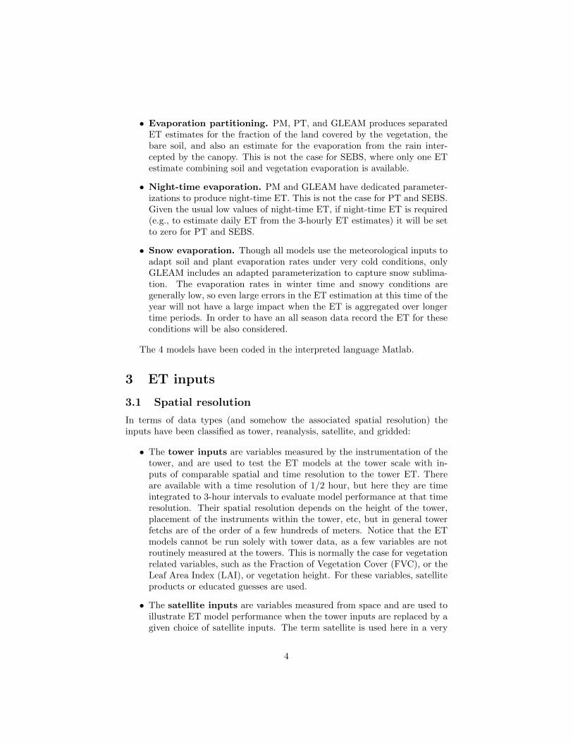
• Evaporation partitioning. PM, PT, and GLEAM produces separatedET estimates for the fraction of the land covered by the vegetation, thebare soil, and also an estimate for the evaporation from the rain inter-cepted by the canopy. This is not the case for SEBS, where only one ETestimate combining soil and vegetation evaporation is available.

• Night-time evaporation. PM and GLEAM have dedicated parameter-izations to produce night-time ET. This is not the case for PT and SEBS.Given the usual low values of night-time ET, if night-time ET is required(e.g., to estimate daily ET from the 3-hourly ET estimates) it will be setto zero for PT and SEBS.

• Snow evaporation. Though all models use the meteorological inputs toadapt soil and plant evaporation rates under very cold conditions, onlyGLEAM includes an adapted parameterization to capture snow sublima-tion. The evaporation rates in winter time and snowy conditions aregenerally low, so even large errors in the ET estimation at this time of theyear will not have a large impact when the ET is aggregated over longertime periods. In order to have an all season data record the ET for theseconditions will be also considered.

The 4 models have been coded in the interpreted language Matlab.

3 ET inputs

3.1 Spatial resolution

In terms of data types (and somehow the associated spatial resolution) theinputs have been classified as tower, reanalysis, satellite, and gridded:

• The tower inputs are variables measured by the instrumentation of thetower, and are used to test the ET models at the tower scale with in-puts of comparable spatial and time resolution to the tower ET. Thereare available with a time resolution of 1/2 hour, but here they are timeintegrated to 3-hour intervals to evaluate model performance at that timeresolution. Their spatial resolution depends on the height of the tower,placement of the instruments within the tower, etc, but in general towerfetchs are of the order of a few hundreds of meters. Notice that the ETmodels cannot be run solely with tower data, as a few variables are notroutinely measured at the towers. This is normally the case for vegetationrelated variables, such as the Fraction of Vegetation Cover (FVC), or theLeaf Area Index (LAI), or vegetation height. For these variables, satelliteproducts or educated guesses are used.

• The satellite inputs are variables measured from space and are used toillustrate ET model performance when the tower inputs are replaced by agiven choice of satellite inputs. The term satellite is used here in a very

4

loose way, as some of the inputs are coming from the ERA-Interim reanal-ysis where typically a large suite of meteo observations (ground network,radiosondes, satellites, etc) are assimilated into a physical model to derivean estimate of a given variable. Their spatial and time resolutions candiffer vastly between products (from the ∼1 km project LAI to the ∼100km SRB net radiation product), and can be quite different from the towerfetch. Therefore the ET estimated from the models represents an esti-mate where different spatial and time resolutions are combined, in nearlyall cases at poorer resolutions that the tower ET.

• The reanalysis inputs are variables derived from the ERA-Interim re-analysis. As indicated above, some of the inputs used here come fromthis reanalysis, and as turbulent fluxes are also output by ERA-Interim,there may be an interest in comparing our ET models running with thereanalysis inputs with the ERA-Interim ET. Notice that the satellite runsalso use ERA-Interim, but only for the meteorology. Here all inputs butthe vegetation are from the reanalysis (e.g., also the surface radiation, sur-face temperature, precipitation, etc). The spatial resolution of the ERA-Interim inputs corresponds to the grid of their physical model (∼75km),which is much larger than the typical tower fetch. Estimates from theforecast exist every 3 hours.

• The gridded inputs are the satellite inputs gridded at a common spa-tial and time resolution to allow running the ET models at continentalscales. For instance, the wind used in the satellite inputs was the originalERA-Interim wind at ∼75 km, while now the wind field has been griddedto a resolution of ∼25 km. Another example: LAI at a satellite input hasa resolution of ∼1 km, while here we use the ∼25 km LAI also availableto the project. The gridded inputs are used to evaluate the model per-formance from the global runs by comparing the gridded ET estimatesfrom a given gridded cell with the ET fluxes from towers located at thatcell. Compared with the satellite inputs, all inputs are now at a commonspatial resolution, though the inherent original spatial resolution of theinputs still plays a role in the “true” resolution of the products. The grid-ding has been done by simple linear interpolations if the original resolutionwas larger than the gridded resolution, nearest neighbour matching if theywere of comparable resolution, or spatial averages if the original resolutionwas much finer than the gridded resolution. An exception is land cover,where spatial upscaling is done by selecting the dominant cover.

In-situ estimates of ET at large spatial resolutions are not routinely available,so the ET model estimates run with the different inputs are always comparedwith the same tower ET. The best model performance for an evaluation with thetower ET is then expected to happen when the models are run with the towerinputs, and an expected degradation in model performance is likely to happenwhen the ET models are run with the other inputs. On the one hand, whenthe spatial resolution of the inputs starts to differ from the tower fetch, the ET

5

at the tower will be less representative of the modeled ET. The degradationin model performance (as compared with the tower ET) will be more or lesssevere depending on surface heterogeneity around the tower. On the otherhand, the satellite inputs are likely to have larger errors compared with thein-situ measurements at the tower. Therefore it could be expected that satelliteinputs are capturing the physical processes at the tower less accurately than thein-situ observations at the tower, resulting in lower ET model performance dueto more uncertain inputs.

3.2 Time resolution

In terms of time resolution, the tower data is available at 1/2 hour intervalsand has been time-integrated to 3-hourly in order to run the ET models with3-hourly inputs. The 3-hourly inputs have also been aggregated to daily valuesin order to run the models with daily inputs. The remaining data has beentime-matched to the 3-hourly or daily resolutions from their native resolutionin different ways depending on the type of data and original resolution. Forinstance, the vegetation products have an 8-day time resolution, and the 8-dayvalue is assigned to all 3-hourly intervals in that period.

It should be noted that the tower data record is not time-continuous asin some occasions there are no measurements. This is not a problem for thePM, PT, and SEBS models because the ET estimation depends only on aninstantaneous atmospheric/surface state. When inputs to the models and/orET for the evaluation are missing those 3 models are not run. GLEAM isdifferent as it operates as a small hydrological model requiring continuous datarecords. To facilitate running GLEAM the tower inputs have been gap-filledwith ERA-Interim data, though as before only the time instants where thetower data existed are used for the model evaluation.

3.3 Tower LST

The tower LST is derived from the longwave radiometer measurements at thetower by inverting the equation relating the upwelling spectral radiance mea-sured by the radiometer and the LST. If LWout and LWin are the upwellingand downwelling longwave radiation, respectively, ε is the broadband emissivityof the Earth surface in the spectral range of measurements, and σ is the StefanBoltzman constant, the equation to derive the LST takes the form:

LWout = ( 1 - ε) LWin + ε σ LST4

The broadband emissivity is estimated from the MODIS-based Global InfraredLand Surface Emissivity Database [Seemann et al., 2008] operated by the Co-operative Institute for Meteorological Satellite Studies (CIMSS). The estimatesare calculated by following the approach suggested by Wang et al. [2005] usingthe following linear combination of narrowband emissivities at 8.5, 11, and 12

6

µm:

ε = 0.2122 ε8.5 + 0.3859 ε11 + 0.4029 ε12

3.4 LAI/FAPAR model adaptation

Given that the PT, PM, and SEBS models have been run in the past withvegetation products derived from MODIS, a direct application of the projectTIP-derived LAI and FAPAR is not possible (the reader is referred to theproject LAI/FAPAR Validation Report for more details). Therefore we haveundertaken a biome-based calibration between the MODIS LAI/FAPAR 8-days1 km product MOD15A2 and the WACMOS-ET TIP-based LAI/FAPAR in or-der to keep the dynamics of the WACMOS-ET product but with the absolutevalues expected from a MODIS-like LAI/FAPAR. The resulting product will bereferred to as WACMOS-ET ”MODIS-like” LAI/FAPAR.

For the tower runs the calibration is local, i.e., a linear regression betweenthe MOD15A2 and the TIP values co-registered at each tower is carried out,followed by an application of the local regression coefficients to the WACMOS-ET LAI/FAPAR time series to produce the MODIS-like LAI/FAPAR. Figure 1gives examples of the products at two towers. CA-Qfo is a station in a evergreenneedle forest and the MOD15A2 and WACMOS-ET LAI/FAPAR absolute val-ues differ considerably. This is expectd as allowing some form of horizontalclumping (MODIS 3D radiative transfer scheme) or not (TIP 1-D) for thesecanopies can result in large differences in the estimated LAI/FAPAR. It can beseen that the local calibration of the MODIS-like product retains the dynamicsof the WACMOS-ET product while adding absolute values close to the MODISproduct. US-Bkg is situated in a cropland area, where the effects of clumpingare much less attenuated, and the different LAI/FAPAR values are much closer.

For the global LAI/FAPAR, the calibration is biome/climate based. Theminimum and maximum near-surface air temperature and relative humidity(Tmin, Tmax, and RH, respectively) for all the pixels falling in a given biomeare collected and a mean Tmin, Tmax, and RH per biome are estimated. Thesemean values are used to prepare a sub-biome classification of the pixels (a givenpixel is associated to a given sub-class depending on the pixel mean Tmin,Tmax, and RH being below or above the biome mean values). For each of thesub-biomes a linear regression between MOD15A2 and WACMOS-ET LAI andFAPAR is calculated and the regression coeffcients applied to each pixel (fallingin that sub-biome) time series of WACMOS-ET values to derive the MODIS-likeLAI/FAPAR.

7

Figure 1: 2005-2006 time series of MODIS MOD15A2 LAI and FAPAR,WACMOS-ET LAI and FAPAR, and the WACMOS-ET MODIS-like LAI andFAPAR (referred to as calibrated in the figures) at the Canadian tower stationCA-Qfo (top two panels) and the US tower US-Bkg (bottom two panels).

8

4 ET generation at tower scale

4.1 Tower selection

Dedicated runs at tower scale are produced by running the four ET models overa sub-set of towers extracted from FLUXNET La Thuille synthesis data set(http://fluxnet.ornl.gov). The tower selection was driven by the need of havingET fluxes and relevant tower inputs to run the models in the project period of2005-2007, and it has resulted in the data set of 24 stations described in Table 1.While some meteorological variables such as near-surface air temperature orhumidity are measured at nearly all towers, some other inputs such as thesurface net radiation or the ground flux, which are key variables to run the ETmodels, are measured at a much more limited number of towers. Some stationsthat were very close to the shore or in places with regular flooding have alsobeen discarded as not being representative of land conditions for the whole year.The final selection certainly does not result in a very large number of towers, butthey represent a significant number of biomes and climates, with a reasonablesample of dry-wet conditions.

The length of the data record varies from station to station. For the stationsselected only data in 2005-2006 exist. Figure 2 summarizes the existing data byplotting the daily ET derived from the eddy covariance latent flux measurementsat the different towers. Notice that the models will be evaluated only for nonrainy conditions under the assumption that eddy covariance measurements atthe tower are not reliable under rain. Only days with no rain at any of the3-hour intervals are kept for the evaluation.

Concerning the times selected for the evaluation, in order to sample all towerdata at the same times independent of tower location, the 0-3-...21 3-hourlyintervals are selected in local time. For the data existing every 3-hours in UTCtime, time-matching to the 3-hourly tower intervals has been done by a linearinterpolation in time to the 3-hourly local time intervals.

4.2 Tower surface energy balance

In principle the surface energy balance should close at the tower. This is rarelythe case: a lack of closure in the surface energy balance of about 10 - 30% iscommonly found when using Eddy Covariance (EC) techniques to measure theturbulent fluxes (see e.g., Foken [2006]). In practical terms this means that theuncertainty associated to the absolute ET reported by the EC measurementsis relatively large and care should be taken when reporting biases between thetower ET and the ET estimates at the tower.

Given this common lack of energy closure at the tower, the modeled ETis compared with the EC observations but also with the tower ET estimatesderived by imposing energy closure at the tower, i.e., the latent flux should beequal to the surface net radiation minus the turbulent sensible and ground fluxesalso observed at the tower. These estimates are referred to as Energy Residual(ER) ET.

9

Table 1: Stations selected to run the models with tower inputs. From leftto right the station name; longitude; latitude; Koppen-Geiger Climate Classi-fication (KGCC); International Geosphere-Biosphere International Programme(IGBP) land cover; total number of days with data / no precipitation number ofdays with data; evaporative fraction for the DJF, MAM, JJA, SON 3-monthlyperiods.

Name Lon Lat KGCC IGBP Days EFAU-How 131.15E 12.49S Aw SV 114 / 100 0.7/0.7/0.5/0.3CA-Ojp 104.69W 53.92N Dfc ENF 126 / 101 0.2/0.1/0.3/0.5CA-Qfo 74.34W 49.69N Dfc ENF 253 / 166 0.1/0.1/0.4/0.4DE-Geb 10.91E 51.1N Cfb CRO 188 / 113 0.0/0.4/0.5/0.7DE-Har 7.6E0 47.93N Cfb MF 105 / 88 1.0/0.5/0.5/0.7DE-Kli 13.52E 50.89N Cfb CRO 275 / 98 0.0/0.5/0.5/0.0DE-Meh 13.52E 50.89N Cfb CRO 444 / 269 0.0/0.3/0.5/0.5DE-Wet 11.46E 50.45N Cfb ENF 384 / 182 0.1/0.3/0.4/0.6IT-MBo 11.08E 46.03N Dfb MF 149 / 126 0.0/0.6/0.7/0.9IT-Noe 8.15E 40.6N Csa WL 182 / 182 0.7/0.3/0.2/0.3NL-Ca1 4.93E 51.97N Cfb CRO 38 / 22 1.0/0.6/0.6/0.9PT-Mi2 8.02W 38.48N Csa SV 275 / 221 0.5/0.4/0.3/0.4RU-Fyo 32.92E 56.46N Dfb MF 374 / 216 0.0/0.4/0.5/0.4US-ARM 97.49W 36.61N Cfa CRO 159 / 131 0.4/0.5/0.3/0.3US-Aud 110.51W 31.59N BSk OSH 219 / 219 0.5/0.2/0.3/0.5US-Bkg 96.84W 44.35N Dfa CRO 174 / 172 0.6/0.7/0.9/1.0US-Bo2 88.29W 40.01N Dfa CRO 192 / 192 0.3/0.3/0.6/0.3US-FPe 105.1W 48.31N BSk GRA 184 / 184 1.0/0.4/0.6/0.4US-Goo 89.87W 34.25N Cfa CRO 183 / 179 0.7/0.6/0.5/0.6US-MOz 92.2W 38.74N Cfa DBF 252 / 252 0.3/0.4/0.5/0.5US-SRM 110.87W 31.82N BSk OSH 139 / 137 0.2/0.1/0.3/0.4US-WCr 90.08W 45.81N Dfb DBF 338 / 239 0.1/0.2/0.6/0.4US-Wkg 109.94W 31.74N BSk GRA 137 / 137 0.2/0.1/0.2/0.3US-Wrc 121.95W 45.82N Csb ENF 146 / 107 0.4/0.3/0.3/0.5

10

Figure 2: 2005-2006 measured eddy covariance ET in mm/day at the 24 stationswhere the models are run with tower inputs.

11

4.3 Model considerations

As discussed in Section 2, only PM and GLEAM specifically deal with nighttimeevaporation. Nevertheless, nighttime values are required from all models tointegrate the 3-hourly ET estimates to daily values. As indicated in Section 2 thenighttime values are set to zero for SEBS and PT to allow the daily integration.To separate day and night, daylight times are identified by calculating the solarzenith angle, and time intervals where the cosine of the zenith angle is largerthan 0.2 are kept as day values.

SEBS is the only model that requires LST as an input. Strictly speakingthe tower run with satellite inputs should use a satellite LST. However, dueto cloudiness, revisiting time and satellite overpass (for AATSR), and missingdata (for the geostationary LST), the number of 3-hourly LSTs at the stationsreduces drastically (compared with the tower LST derived from the radiometricobservations at the tower). As the general ET evaluation at the tower is doneover 3-hourly and daily values where all models output ET, using the satelliteLST removes a large number of ET values from the analysis. Therefore we usetower LST for the SEBS satellite runs. However, a special run for SEBS usingagain the satellite inputs but now with the LST at the tower from AATSR andthe geosatellite observations is also produced separately from the satellite runusing tower LST.

4.4 ET production at tower scale

Summarising, the different model forcings and time integrations results in thefollowing 3-hourly ET estimates:

• Tower run. ET generated by the 4 models run with the tower data(surface radiation; LST, air temperature, humidity, and wind speed; pre-cipitation) complemented with MODIS LAI/FAPAR, and WACMOS soilmoisture.

• ERA run. ET generated by the 4 models run with the ERA-Interimreanalysis data for all inputs (surface radiation; surface temperature, airtemperature and wind speed; precipitation; soil moisture) complementedwith MODIS LAI/FAPAR.

• Sat-MODIS run. ET generated by the 4 models run with the satellitedata (tower LST; SRB surface radiation; ERA-Interim air temperature,humidity, and wind speed; CMORPH precipitation; WACMOS soil mois-ture) using MODIS products for LAI/FAPAR.

• Sat-WACMOS run. As before but with the WACMOS-ET MODIS-likeproducts processed as indicated in Section 3.4. Notice that both runs areidentical for GLEAM, as GLEAM does not use LAI/FAPAR.

• LST runs. ET generated by SEBS with the satellite inputs as above,with MODIS products for vegetation, and different LST products (fromthe tower, AATSR, and MSG, GOES, or MTSAT depending on location).

12

The ET estimates from these runs are available at 3-hourly, as daily valuesfrom the time-integration of the 3-hourly ET estimates, and as daily values fromrunning the models with the inputs time-integrated from 3-hourly to daily.

5 ET generation at regional scale

5.1 ET inputs

ET at the finest spatial resolution allowed by the RIDS is produced over an areain Europe of ∼500 x 600 km2 (tile h18v04). Figure 3 shows the location of thearea and its IGBP land cover.

ET is generated at 2 spatial resolutions:

• 1 km product. For these runs the ERA-Interim surface radiation, near-surface air temperature, and humidity are replaced by hourly outputs fromthe NWP model COSMO, downscaled from the original resolution of ∼7km to 1 km. The 1 km AATSR product is used for surface temperature,and the 1 km WACMOS-ET MODIS-like LAI/FAPAR characterizes thevegetation.

• 5 km product. As before, but with the COSMO metorological inputsdownscaled to 5 km, the surface temperature from MSG, and the sameLAI/FAPAR but from the 5 km product.

5.2 ET models

Only the PT, PM, and SEBS are run at this spatial scale as they can be appliedwith existing observations from visible and infrared sensors at this fine scale.For GLEAM, key inputs such as the precipitation, soil moisture, and vegetationoptical depth, are based on microwave observations with a spatial resolutionclose to the resolution of the continental runs (∼25 km). In principle, theseinputs could be downscaled to 1 km and GLEAM run over the same areas asthe other models, but given the difference in the ”true” resolution of these inputsand the targeted 1 km resolution, runs of GLEAM at 1 km are not prepared.

5.3 ET evaluation

Evaluation of the regional is mainly done by comparing the runs at differentresolutions. The region includes the sub-catchment of Rietholzbach, managedby one of the consortium members. A lysimeter there provides ET measure-ments representative of the Rietholzbach catchment, and that will be used inthe analyses as in situ data.

13

Figure 3: Area selected for the regional runs, displaying the IGBP land coverof the area (ENF: evergreen needleleaf forest; EBF: evergreen broadleaf forest;DNF: deciduous needleleaf forest; DBF: deciduous broadleaf forest; MF: mixedforest; WL: woody savannas; SV: savannas; CSH: closed shrubland; OSH: openshrubland; Grass: grassland, urban and built-up, barren or sparsely vegetated;Crop: cropland). The red mark shows the location of the Rietholzbach catch-ment.

14

6 ET generation at continental scale

6.1 ET production

The continental scale runs are produced by running the four models with 3-hourly (UTC) gridded inputs on the project sinusoidal grid of ∼25 km. The3-hourly ET estimates from PT, PM, and GLEAM, are also integrated to daily,monthly, and yearly values. An example of ET estimates for Day-Of-the-Year(DOY) 125 in 2007 for PT, PM, and GLEAM is given in Figure 4.

To run SEBS over all the continental surfaces AATSR is selected due to theirglobal coverage, with its 1 km LST upscaled to 25 km by simple spatial averagesand the ERA-Interim near surface meteorology linearly interpolated in time tothe satellite overpass (∼10 am local time) from the closest UTC 3-hourly times.Although some techniques could be used to upscale from local overpass ET todaily ET (e.g., by assuming a day constant evaporative fraction as in Vinukolluet al. [2011]), this has not been pursued here, and no daily, monthly, or yearlyET from SEBS is produced. An example of SEBS ET at AATSR overpass (∼10am) for the same day of Figure 4 is given in Figure 5.

Summarizing, the following ET estimates are generated:

• 3-hourly ET for all continental surfaces applying the PT, PM, and GLEAMmodels, also time integrated to daily, monthly, and yearly values.

• ∼10 am SEBS ET for all continental surfaces when AATSR LST observa-tions are available.

6.2 ET for in-situ evaluation

In terms of evaluation, both in situ tower flux observations, global ET esti-mations from other products, and catchment water balance estimates at ma-jor basins were considered. Regarding the tower records, 187 towers from LaThuile data set were found to have ET observations in the 2005-2007 period.From those, only 95 have been retained imposing two conditions (1) the towerwas not an area of regular flooding, and was not close to water bodies, and (2)at least 30 non-rainy days existed to evaluate the ET gridded estimates. TheGlobCover classification was used to decide about the flooding/water conditions.The final tower selection is listed in Tables 2 and 3.

6.3 ET for global evaluation

For an evaluation at global scale, other ET products at different time and spaceresolutions have been collected. They include models that have been the basisfor the ET algorithms implemented by the project, together with other globaldata sets build in different ways. There are listed here:

• The MODIS ET product (MOD16, Su et al. [2011]), at a resolution of 8days, ∼1 km. This is the basis of the PM algorithm implemented in the

15

Figure 4: PM, PT, and GLEAM ET in mm/day for DOY 125 in 2007.

16

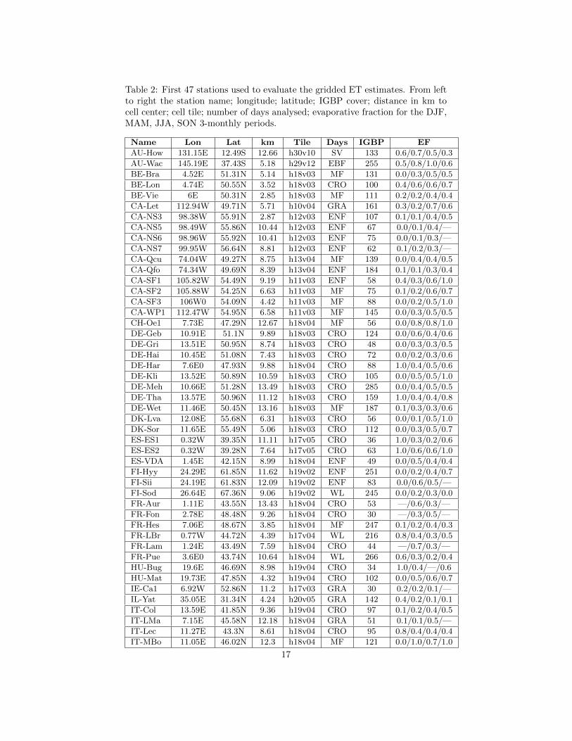
Table 2: First 47 stations used to evaluate the gridded ET estimates. From leftto right the station name; longitude; latitude; IGBP cover; distance in km tocell center; cell tile; number of days analysed; evaporative fraction for the DJF,MAM, JJA, SON 3-monthly periods.

Name Lon Lat km Tile Days IGBP EF

AU-How 131.15E 12.49S 12.66 h30v10 SV 133 0.6/0.7/0.5/0.3

AU-Wac 145.19E 37.43S 5.18 h29v12 EBF 255 0.5/0.8/1.0/0.6

BE-Bra 4.52E 51.31N 5.14 h18v03 MF 131 0.0/0.3/0.5/0.5

BE-Lon 4.74E 50.55N 3.52 h18v03 CRO 100 0.4/0.6/0.6/0.7

BE-Vie 6E 50.31N 2.85 h18v03 MF 111 0.2/0.2/0.4/0.4

CA-Let 112.94W 49.71N 5.71 h10v04 GRA 161 0.3/0.2/0.7/0.6

CA-NS3 98.38W 55.91N 2.87 h12v03 ENF 107 0.1/0.1/0.4/0.5

CA-NS5 98.49W 55.86N 10.44 h12v03 ENF 67 0.0/0.1/0.4/—

CA-NS6 98.96W 55.92N 10.41 h12v03 ENF 75 0.0/0.1/0.3/—

CA-NS7 99.95W 56.64N 8.81 h12v03 ENF 62 0.1/0.2/0.3/—

CA-Qcu 74.04W 49.27N 8.75 h13v04 MF 139 0.0/0.4/0.4/0.5

CA-Qfo 74.34W 49.69N 8.39 h13v04 ENF 184 0.1/0.1/0.3/0.4

CA-SF1 105.82W 54.49N 9.19 h11v03 ENF 58 0.4/0.3/0.6/1.0

CA-SF2 105.88W 54.25N 6.63 h11v03 MF 75 0.1/0.2/0.6/0.7

CA-SF3 106W0 54.09N 4.42 h11v03 MF 88 0.0/0.2/0.5/1.0

CA-WP1 112.47W 54.95N 6.58 h11v03 MF 145 0.0/0.3/0.5/0.5

CH-Oe1 7.73E 47.29N 12.67 h18v04 MF 56 0.0/0.8/0.8/1.0

DE-Geb 10.91E 51.1N 9.89 h18v03 CRO 124 0.0/0.6/0.4/0.6

DE-Gri 13.51E 50.95N 8.74 h18v03 CRO 48 0.0/0.3/0.3/0.5

DE-Hai 10.45E 51.08N 7.43 h18v03 CRO 72 0.0/0.2/0.3/0.6

DE-Har 7.6E0 47.93N 9.88 h18v04 CRO 88 1.0/0.4/0.5/0.6

DE-Kli 13.52E 50.89N 10.59 h18v03 CRO 105 0.0/0.5/0.5/1.0

DE-Meh 10.66E 51.28N 13.49 h18v03 CRO 285 0.0/0.4/0.5/0.5

DE-Tha 13.57E 50.96N 11.12 h18v03 CRO 159 1.0/0.4/0.4/0.8

DE-Wet 11.46E 50.45N 13.16 h18v03 MF 187 0.1/0.3/0.3/0.6

DK-Lva 12.08E 55.68N 6.31 h18v03 CRO 56 0.0/0.1/0.5/1.0

DK-Sor 11.65E 55.49N 5.06 h18v03 CRO 112 0.0/0.3/0.5/0.7

ES-ES1 0.32W 39.35N 11.11 h17v05 CRO 36 1.0/0.3/0.2/0.6

ES-ES2 0.32W 39.28N 7.64 h17v05 CRO 63 1.0/0.6/0.6/1.0

ES-VDA 1.45E 42.15N 8.99 h18v04 ENF 49 0.0/0.5/0.4/0.4

FI-Hyy 24.29E 61.85N 11.62 h19v02 ENF 251 0.0/0.2/0.4/0.7

FI-Sii 24.19E 61.83N 12.09 h19v02 ENF 83 0.0/0.6/0.5/—

FI-Sod 26.64E 67.36N 9.06 h19v02 WL 245 0.0/0.2/0.3/0.0

FR-Aur 1.11E 43.55N 13.43 h18v04 CRO 53 —/0.6/0.3/—

FR-Fon 2.78E 48.48N 9.26 h18v04 CRO 30 —/0.3/0.5/—

FR-Hes 7.06E 48.67N 3.85 h18v04 MF 247 0.1/0.2/0.4/0.3

FR-LBr 0.77W 44.72N 4.39 h17v04 WL 216 0.8/0.4/0.3/0.5

FR-Lam 1.24E 43.49N 7.59 h18v04 CRO 44 —/0.7/0.3/—

FR-Pue 3.6E0 43.74N 10.64 h18v04 WL 266 0.6/0.3/0.2/0.4

HU-Bug 19.6E 46.69N 8.98 h19v04 CRO 34 1.0/0.4/—/0.6

HU-Mat 19.73E 47.85N 4.32 h19v04 CRO 102 0.0/0.5/0.6/0.7

IE-Ca1 6.92W 52.86N 11.2 h17v03 GRA 30 0.2/0.2/0.1/—

IL-Yat 35.05E 31.34N 4.24 h20v05 GRA 142 0.4/0.2/0.1/0.1

IT-Col 13.59E 41.85N 9.36 h19v04 CRO 97 0.1/0.2/0.4/0.5

IT-LMa 7.15E 45.58N 12.18 h18v04 GRA 51 0.1/0.1/0.5/—

IT-Lec 11.27E 43.3N 8.61 h18v04 CRO 95 0.8/0.4/0.4/0.4

IT-MBo 11.05E 46.02N 12.3 h18v04 MF 121 0.0/1.0/0.7/1.0

17

Table 3: Remaining 48 stations used to evaluate the gridded ET estimates.From left to right the station name; longitude; latitude; IGBP cover; distancein km to cell center; cell tile; number of days analysed; evaporative fraction forthe DJF, MAM, JJA, SON 3-monthly periods.

Name Lon Lat km Tile Days IGBP EF

IT-Non 11.09E 44.69N 7.91 h18v04 CRO 56 0.4/0.5/0.7/—

IT-Ro1 11.93E 42.41N 5.06 h18v04 CRO 260 0.1/0.3/0.4/0.4

IT-Ro2 11.92E 42.39N 5.66 h18v04 CRO 160 0.0/0.3/0.5/0.4

IT-Vig 8.85E 45.32N 8.68 h18v04 CRO 55 1.0/0.5/0.8/0.5

NL-Hor 5.07E 52.03N 12.48 h18v03 GRA 81 0.0/0.5/0.6/1.0

NL-Lan 4.9E0 51.95N 2.85 h18v03 GRA 36 0.3/0.6/0.6/1.0

NL-Loo 5.74E 52.17N 9.60 h18v03 CRO 168 0.5/0.3/0.3/0.4

PT-Esp 8.6W0 38.64N 5.90 h17v05 WL 39 0.4/0.3/0.2/0.2

PT-Mi1 8W 38.54N 15.06 h17v05 CRO 90 0.2/0.2/0.1/0.0

PT-Mi2 8.02W 38.48N 8.79 h17v05 CRO 233 0.8/0.4/0.2/0.3

SE-Faj 13.55E 56.27N 14.45 h18v03 MF 39 0.8/0.3/0.4/—

UK-Ham 0.86W 51.12N 3.51 h17v03 CRO 66 0.2/0.2/0.4/0.3

UK-PL3 1.27W 51.45N 12.69 h17v03 CRO 193 0.0/0.3/0.5/0.9

US-ARM 97.49W 36.61N 9.60 h10v05 CRO 155 0.6/0.5/0.3/0.3

US-Arb 98.04W 35.55N 11.64 h10v05 GRA 45 0.2/0.4/0.7/0.5

US-Aud 110.51W 31.59N 11.53 h08v05 GRA 228 0.8/0.1/0.2/0.7

US-Bkg 96.84W 44.35N 11.26 h11v04 CRO 195 1.0/0.8/0.8/1.0

US-Blo 120.63W 38.9N 10.81 h08v05 ENF 155 0.6/0.4/0.6/0.6

US-FPe 105.1W 48.31N 13.31 h10v04 GRA 188 0.0/0.4/0.3/0.6

US-Fmf 111.73W 35.14N 7.09 h08v05 WL 99 0.1/0.3/0.3/0.3

US-Fuf 111.76W 35.09N 8.98 h08v05 WL 69 0.1/0.2/0.4/0.2

US-Fwf 111.77W 35.45N 9.21 h08v05 OSH 119 0.2/0.2/0.4/0.4

US-Goo 89.87W 34.25N 1.80 h10v05 WL 208 0.9/0.6/0.5/0.7

US-IB1 88.22W 41.86N 12.46 h11v04 GRA 165 1.0/0.4/0.6/0.4

US-IB2 88.24W 41.84N 12.01 h11v04 GRA 218 0.3/0.4/0.7/0.5

US-Los 89.98W 46.08N 9.39 h11v04 MF 83 0.1/0.2/0.5/0.4

US-MOz 92.2W 38.74N 11.47 h10v05 CRO 286 0.3/0.4/0.5/0.5

US-NC1 76.71W 35.81N 13.24 h11v05 CRO 169 0.5/0.5/0.8/0.7

US-NC2 76.67W 35.8N 9.96 h11v05 CRO 240 0.5/0.5/0.8/0.8

US-SO2 116.62W 33.37N 10.99 h08v05 OSH 133 0.7/0.4/0.2/0.2

US-SO3 116.62W 33.38N 10.77 h08v05 OSH 89 0.9/0.4/0.2/0.2

US-SO4 116.64W 33.38N 9.01 h08v05 OSH 153 0.4/0.3/0.2/0.2

US-SP1 82.22W 29.74N 9.85 h10v06 WL 182 0.3/0.3/0.4/0.4

US-SRM 110.87W 31.82N 5.93 h08v05 OSH 159 0.2/0.1/0.1/0.4

US-Syv 89.35W 46.24N 13.7 h11v04 MF 163 0.1/0.2/0.5/—

US-WCr 90.08W 45.81N 11.4 h11v04 MF 251 0.1/0.2/0.6/0.4

US-Wkg 109.94W 31.74N 5.14 h08v05 OSH 154 0.2/0.1/0.1/0.3

US-Wrc 121.95W 45.82N 10.53 h09v04 ENF 74 0.3/0.3/0.3/—

US-NC2 76.67W 35.8N 9.96 h11v05 CRO 240 0.5/0.5/0.8/0.8

US-SO2 116.62W 33.37N 10.99 h08v05 OSH 133 0.7/0.4/0.2/0.2

US-SO3 116.62W 33.38N 10.77 h08v05 OSH 89 0.9/0.4/0.2/0.2

US-SO4 116.64W 33.38N 9.01 h08v05 OSH 153 0.4/0.3/0.2/0.2

US-SP1 82.22W 29.74N 9.85 h10v06 WL 182 0.3/0.3/0.4/0.4

US-SRM 110.87W 31.82N 5.93 h08v05 OSH 159 0.2/0.1/0.1/0.4

US-Syv 89.35W 46.24N 13.7 h11v04 MF 163 0.1/0.2/0.5/—

US-WCr 90.08W 45.81N 11.4 h11v04 MF 251 0.1/0.2/0.6/0.4

US-Wkg 109.94W 31.74N 5.14 h08v05 OSH 154 0.2/0.1/0.1/0.3

US-Wrc 121.95W 45.82N 10.53 h09v04 ENF 74 0.3/0.3/0.3/—

18

Figure 5: SEBS ET in mm/3-hours at the AATSR overpass of ∼10 am for DOY125 in 2007.

project, but MOD16 uses different GMAO-MERRA and MODIS basedproducts as model forcings.

• The PT-JPL product driven with SRB surface radiation, GIMMS NDVI,and CRU meteorological data [Fisher et al., 2008], produced as monthlyestimates at 1o. This is the basis of the PT model implemented in theproject.

• The GLEAM v2A product, daily at 0.25o[Miralles et al., 2011b,a], whichis the basis of the 3-hourly GLEAM run by the project. It uses ERA-Interim surface radiation and CPC-unified precipitation, and ISCCP+AIRSair temperature (soil moisture and vegetaion optical depth with the sameinputs applied here).

• The LandFlux-EVAL benchmark data set [Mueller et al., 2013], a multi-model ensemble including observation-based data sets, land-surface modeldata and re-analyses data, at 0.5oand monthly.

• The ERA-interim reanalysis latent fluxes from the forecast fields at 3-hourly and ∼75 km.

• The MPI-MTE product, a global empirical upscaling of FLUXNET eddycovariance observations [Jung et al., 2009].

6.4 ET for basin-integrated evaluation

Globally distributed long-term and annually resolved river discharge data forbasins larger than 10000 km2 with corresponding watershed boundaries wereobtained from the Global Runoff Data Centre. Watershed boundaries were used

19

to extract net radiation from CERES, mean annual precipitation for the targetperiod 2005-2007 from the GPCP, and GPCC v6 products. Two versions ofGPCC v6 were processed by applying relative gauge correction factors accordingto Fuchs et al. [2001] and Legates and Willmott [1990] to the native GPCCproducts as recommended by the producers.

River discharge was converted from m3/s to mm/yr based on the GRDCreported basin area - we excluded basins where the absolute difference betweenGRDC reported area and area calculated from basin boundaries exceeded 25%.We further discarded basins where the uncertainty of the precipitation productsis large by filtering out those with an on average very low density of rain gauges(< 0.1 per 0.5 degree gridcell) or frequent snow fall (> 25 days per year; basedon CLOUDSAT). Few basins were further excluded where ETP-Q < 0 or LEP-Q > Rn. Discharge data were often not available for the years 2005-2007. Theintroduced uncertainty of mean annual watershed ET due to a different referenceperiods of runoff and precipitation is small in comparison to the uncertaintiesof precipitation and basin areas. Nevertheless, we used a robust regressionapproach between GPCC precipitation and measured runoff for the overlappingperiod (which is always at least 10 years) to estimate runoff for the missing yearsto account for the possibility of a trend in runoff due to a trend in precipitation.

Few basins were further excluded where ETP-Q < 0 or LEP-Q > Rn. Be-cause few basins showed still implausible runoff values we trained a machinelearning algorithm (Random Forests, Breimann 2001)) to predict mean annualrunoff from mean annual precipitation and mean annual net radiation, and re-moved outlier basins. Outliers were identified according to a common procedureby checking if the absolute predicted minus observed runoff value exceeded threetime the inter-quartile range of residuals.

The resulting record of 900 basins were clustered in 30 classes based onprecipitation (log transformed), net radiation, and evaporative fraction (EF= ET/Rn) to reduce noise and retain clear patterns for the evaluation. Theclustering algorithm was k-means with the cityblock distance, and variableswere transformed to zero mean and unit variance. Each of the 30 classes wasassigned to one of four groups based on the cluster centroids by splitting intoextra-tropical and tropical using a threshold of Rn = 2500 MJ/m2/yr and intomoist and dry respectively using a threshold of EF = 0.5.

7 Summary

References

JB Fisher, KP Tu, and DD Baldocchi. Global estimates of the land-atmospherewater flux based on monthly AVHRR and ISLSCP-II data, validated at 16FLUXNET sites. Remote Sens. Envir., 112(3):901–919, 2008.

Thomas Foken. 50 Years of the Monin–Obukhov Similarity Theory. Boundary-Layer Meteorology, 119(3):431–447, July 2006.

20

T. Fuchs, J. Rapp, F. Rubel, and B. Rudolf. Correction of Synoptic PrecipitationObservations due to Systematic Measuring Errors with Special Regard toPrecipitation. Phases. Phys.Chem. Earth (B), 26(9):689–693, 2001.

M. Jung, M. Reichstein, and A. Bondeau. Towards global empirical upscaling ofFLUXNET eddy covariance observations: validation of a model tree ensembleapproach using a biosphere model. Biogeosciences Discussion, 6(3):5271–5304, 2009.

D.R. Legates and C.J. Willmott. Mean seasonal and spatial variability in gauge-cor- rected, global precipitation. Int. J. Climatol, 10:11q–127, 1990.

D.G. Miralles, R.A.M. De Jeu, J.H. Gash, T.R.H. Holmes, and A.J. Dolman.Magnitude and variability of land evaporation and its components at theglobal scale. Hydrology and Earth System Sciences, 15(3):967–981, March2011a.

D.G. Miralles, T.R.H. Holmes, R.A.M. De Jeu, J.H. Gash, A.G.C. Meesters, andA.J. Dolman. Global land-surface evaporation estimated from satellite-basedobservations. Hydrol. Earth System Sci., 15(2):453–469, February 2011b.

Q. Mu, M. Zhao, and S.W. Running. Improvements to a MODIS global terres-trial evapotranspiration algorithm. Remote Sens. Envir., 115(8):1781–1800,January 2011.

B. Mueller, M. Hirschi, C. Jimenez, P. Ciais, P. A. Dirmeyer, A. J. Dolman,J. B. Fisher, M. Jung, F. Ludwig, F. Maignan, F. Miralles, M. McCabe,M. Reichstein, J. Shefield, K. C. Wang, E. F. Wood, Y. Zhang, , and S.I.Seneviratne. Benchmark products for land evapotranspiration: LandFlux-EVAL multi- dataset synthesis. HESS, 10:doi:10.5194/hessd 107692013, 2013.

S. W. Seemann, E. E. Borbas, R. O. Knuteson, G. R. Stephenson, and H.-L. Huang. Development of a global infrared surface emissivity database forapplication to clear sky retrievals from multispectral satellite radiance mea-surements. J. Appl. Meteorol. Climat., 47:108–123, 2008.

Z. Su. The Surface Energy Balance System (SEBS) for estimation of turbulentheat fluxes. Hydrology and Earth System Sciences, 6(1):85–99, 2002.

Z. Su, R.A. Roebeling, J. Schulz, I. Holleman, V. Levizzani, W.J. Timmermans,H. Rott, N. Mognard-Campbell, R. De Jeu, and W. Wagner. Observation ofHydrological Processes Using Remote Sensing. Treatise on Water Science,edited by: Wilderer, P., Academic Press, Oxford, 2:351–399, 2011.

R.K. Vinukollu, E.F. Wood, C.R. Ferguson, and J.B. Fisher. Global estimatesof evapotranspiration for climate studies using multi-sensor remote sensingdata: Evaluation of three process-based approaches. Remote Sens. Envir.,115(3):801–823, January 2011.

21

K. Wang, Z. Wan, P. Wang, M. Sparrow, J. Liu, X. Zhou, and S. Haginoya.Estimation of surface long wave radiation and broadband emissiv- ity usingModerate Resolution Imaging Spectroradiometer (MODIS) land surface tem-perature/emissivity products. JGR, 110(D11):DOI:10.1029/2004JD005566,2005.

22