euler equations for the estimation of dynamic discrete...

EULER EQUATIONS FOR THE

ESTIMATION OF DYNAMIC

DISCRETE CHOICE STRUCTURAL

MODELS

Victor Aguirregabiria and Arvind Magesan

ABSTRACT

We derive marginal conditions of optimality (i.e., Euler equations) for ageneral class of Dynamic Discrete Choice (DDC) structural models.These conditions can be used to estimate structural parameters in thesemodels without having to solve for approximate value functions. Thisresult extends to discrete choice models the GMM-Euler equationapproach proposed by Hansen and Singleton (1982) for the estimation ofdynamic continuous decision models. We first show that DDC models canbe represented as models of continuous choice where the decision variableis a vector of choice probabilities. We then prove that the marginal condi-tions of optimality and the envelope conditions required to constructEuler equations are also satisfied in DDC models. The GMM estimationof these Euler equations avoids the curse of dimensionality associated tothe computation of value functions and the explicit integration over thespace of state variables. We present an empirical application and compare

Structural Econometric Models

Advances in Econometrics, Volume 31, 3�44

Copyright r 2013 by Emerald Group Publishing Limited

All rights of reproduction in any form reserved

ISSN: 0731-9053/doi:10.1108/S0731-9053(2013)0000032001

3

http://dx.doi.org/10.1108/S0731-9053(2013)0000032001

estimates using the GMM-Euler equations method with those frommaximum likelihood and two-step methods.

Keywords: Dynamic discrete choice structural models; Eulerequations; choice probabilities

JEL classifications: C35; C51; C61

INTRODUCTION

The estimation of Dynamic Discrete Choice (DDC) structural modelsrequires the computation of expectations (value functions) defined as inte-grals or summations over the space of state variables. In most empiricalapplications, the range of variation of the vector of state variables is contin-uous or discrete with a very large number of values. In these cases theexact solution of expectations or value functions is an intractable problem.To deal with this dimensionality problem, applied researchers use approxi-mation techniques such as discretization, Monte Carlo simulation, polyno-mials, sieves, neural networks, etc.1 These approximation techniques areneeded not only in full-solution estimation techniques but also in any two-step or sequential estimation method that requires the computation of valuefunctions.2 Replacing true expected values with approximations introducesan approximation error, and this error induces a statistical bias in theestimation of the parameter of interests. Though there is a rich literature onthe asymptotic properties of these simulation-based estimators,3 little isknown about how to measure this approximation-induced estimation bias fora given finite sample.4

In this context, the main contribution of this article is in the derivationof marginal conditions of optimality (Euler equations) for a general classof DDC models. We show that these Euler equations provide moment con-ditions that can be used to estimate structural parameters without solvingor approximating value functions. The estimator based on these Eulerequations is not subject to bias induced by the approximation of valuefunctions. Our result extends to discrete choice models the GMM-Eulerequation approach that Hansen and Singleton (1982) proposed for theestimation of dynamic models with continuous decision variables. TheGMM-Euler equation approach has been applied extensively to the estima-tion of dynamic structural models with continuous decision variables, such

4 VICTOR AGUIRREGABIRIA AND ARVIND MAGESAN

as problems of household consumption, savings, and portfolio choices, orfirm investment decisions, among others. The conventional wisdom wasthat this method could not be applied to discrete choice models because,obviously, there are not marginal conditions of optimality with respect todiscrete choice variables. In this article, we show that the optimal decisionrule in a dynamic (or static) discrete choice model can be derived froma decision problem where the choice variables are probabilities that havecontinuous support. Using this representation of a discrete choice model,we obtain Euler equations by combining marginal conditions of optimalityand Envelope Theorem conditions in a similar way as in dynamic modelswith continuous decision variables. Just as in the Hansen�Singletonapproach, these Euler equations can be used to construct moment condi-tions and to estimate the structural parameters of the model by GMMwithout having to evaluate/approximate value functions.

Our derivation of Euler equations for DDC models extends previouswork by Hotz and Miller (1993), Aguirregabiria and Mira (2002), andArcidiacono and Miller (2011). These papers derive representations ofoptimal decision rules using Conditional Choice Probabilities (CCPs) andshow how these representations can be applied to estimate DDC modelsusing simple two-step methods that provide substantial computational sav-ings relative to full-solution methods. In these papers, we can distinguishthree different types of CCP representations of optimal decisions rules:(1) the present-value representation which consists of using CCPs to obtaina closed-form expression for the expected and discounted stream of futurepayoffs associated with each choice alternative; (2) the terminal-state repre-sentation which applies only to optimal stopping problems with a terminalstate; and (3) the finite-dependence representation which was introduced byArcidiacono and Miller (2011) and applies to a particular class of DDCmodels with the finite dependence property.5

Our article presents a new CCP representation that we call CCP-Euler-equation representation. This representation has several advantages overthe previous ones. The present-value representation is the CCP approachmore commonly used in empirical applications because it can be applied toa general class of DDC models. However, that representation requires thecomputation of present values and therefore it is subject to the curse ofdimensionality and to biases induced by approximation error (e.g., discreti-zation, Monte Carlo simulation). The terminal-state, the finite-dependence,and the CCP-Euler-equation representations do not involve the computa-tion of present values, or even the estimation of CCPs at every possiblestate, and this implies substantial computational savings as well as avoiding

5Euler Equations for the Estimation of DDC Structural Models

biases induced by approximation errors. Furthermore, relative to terminal-state and finite-dependence representations, our Euler equation applies to ageneral class of DDC models. We can derive Euler equations for any DDCmodel where the unobservables satisfy the conditions of additive separabil-ity (AS) in the payoff function, and conditional independence (CI) in thetransition of the state variables.

The estimation based on the moment conditions provided by the Eulerequation, or terminal-state, or finite-dependence representations imply anefficiency loss relative to estimation based on present-value representation.As shown by Aguirregabiria and Mira (2002, Proposition 4), the two-steppseudo maximum likelihood (PML) estimator based on the CCP present-value representation is asymptotically efficient (equivalent to the maximumlikelihood (ML) estimator). However, this efficiency property is not sharedby the other CCP representations. Therefore, there is a trade-off in thechoice between CCP estimators based on Euler equations and on present-value representations. The present-value representation is the best choice inmodels that do not require approximation methods. However, in modelswith large state spaces that require approximation methods, the Eulerequations CCP estimator can provide more accurate estimates.

We present an empirical application where we estimate a model offirm investment. We compare estimates using CCP Euler equations, CCPpresent-value, and ML methods.

EULER EQUATIONS IN DYNAMIC

DECISION MODELS

Dynamic Decision Model

Time is discrete and indexed by t. Every period t, an agent chooses anaction at within the set of feasible actions A that, for the moment, can beeither a continuous or a discrete choice set. The agent makes this decision

to maximize his expected intertemporal payoff Et

PT − tj= 0 β

jΠtðatþ j; stþ jÞh i

;

where β∈ ð0; 1Þ is the discount factor, T is the time horizon that can befinite or infinite, Πtð:Þ is the one-period payoff function at period t, and stis the vector of state variables at period t. These state variables followa controlled Markov process, and the transition probability densityfunction at period t is ftðstþ 1jat; stÞ: By Bellman’s principle of optimality,


the sequence of value functions fVtð:Þ : t≥ 1g can be obtained using therecursive expression:

VtðstÞ= maxat ∈A

Πtðat; stÞ þ β

ZVtþ 1ðstþ 1Þ ftðstþ 1 j at; stÞ dstþ 1

� �ð1Þ

The sequence of optimal decision rules fα�t ð:Þ : t≥ 1 are defined as theargmax in at ∈A of the expression within brackets in Eq. (1).

Suppose that the primitives of the model fΠt; ft; βg can be characterizedin terms of vector of structural parameters θ. The researcher has panel datafor N agents (e.g., individuals, firms) over ~T periods of time, with informa-tion on agents’ actions and a subset of the state variables. The estimationproblem is to use these data to consistently estimate the vector of para-meters θ. In this section, we first describe this approach in the context ofcontinuous-choice models, as proposed in the seminal work by Hansen andSingleton (1982). Second, we show how a general class of discrete choicemodels can be represented as continuous choice models where the decisionvariable is a vector of choice probabilities. Finally, we show that it ispossible to construct Euler equations using this alternative representationof discrete choice models, and that these Euler equations can be usedto construct moment conditions and a GMM estimator of the structuralparameters θ.

Euler Equations in Dynamic Continuous Decision Models

Suppose that the decision at is a vector of continuous variables in the K

dimensional Euclidean space: at ∈A⊆RK . The vector of state variables

st ≡ ðyt; ztÞ contains both exogenous (zt) and endogenous (yt) variables.Exogenous state variables follow a stochastic process that does not dependon the agent’s actions fatg, for example, the price of capital in a model offirm investment under the assumption that firms are price takers in thecapital market. In contrast, the evolution over time of the endogenous statevariables, yt, depends on the agent’s actions, for example, the stock of capi-tal in a model of firm investment. More precisely, the transition probabilityfunction of the state variables is

ftðstþ 1 jat; stÞ= 1fytþ 1 =Yðat; st; ztþ 1Þg f zt ðztþ 1 jztÞ ð2Þ

where 1 :f g is the indicator function, Yð:Þ is a vector-valued function thatrepresents the transition rule of the endogenous state variables, and f zt is


the transition density function for the exogenous state variables. For thederivation of Euler equations in a continuous decision model, it is conveni-ent to represent the transition rule of the endogenous state variables usingthe expression 1 ytþ 1 = Yðat; st; ztþ 1Þ

� �. This expression establishes that ytþ 1

is a deterministic function of ðat; st; ztþ 1Þ. However, this structure allows fora stochastic transition in the endogenous state variables because ztþ 1 is anargument of function Yð:Þ.6 The following assumption provides sufficientconditions for the derivation of Euler equations in dynamic continuousdecision models.

Assumption EE-Continuous. (A) The payoff function Πt and the transi-tion function Yð:Þ are continuously differentiable in all their arguments.(B) at and yt are both vectors in the K-dimension Euclidean space andfor any value of ðat; st; ztþ 1Þ we have that

∂Yðat; st; ztþ 1Þ∂y0t

=Hðat; stÞ∂Yðat; st; ztþ 1Þ

∂a0tð3Þ

where Hðat; stÞ is a K ×K matrix.

For the derivation of the Euler equations, we consider the followingconstrained optimization problem. We want to find the decisions rules atperiods t and tþ 1 that maximize the one-period-forward expected profitΠt þ β EtðΠtþ 1Þ under the constraint that the probability distribution of theendogenous state variables ytþ 2 conditional on st implied by the new deci-sion rules αtð:Þ and αtþ 1ð:Þ is identical to that distribution under the optimaldecision rules of our original DP problem, α�t ð:Þ and α�tþ 1ð:Þ. By construc-tion, this optimization problem depends on payoffs at periods t and tþ 1

only, and not on payoffs at tþ 2 and beyond. And by definition of optimaldecision rules, we have that α�t ð:Þ and α�tþ 1ð:Þ should be the optimal solutionsto this constrained optimization problem. For a given value of the statevariables st, we can represent this constrained optimization problem as

max at ; atþ1f g∈A2 Πtðat;stÞþβRΠtþ1ðatþ1;Yðat;st;ztþ1Þ;ztþ1Þ f zt ztþ1jztð Þdztþ1

� �subject to: Yðatþ1;Yðat;st;ztþ1Þ;ztþ1;ztþ2Þ=κ�tþ2ðst;ztþ1;ztþ2Þ

ð4Þwhere Yðatþ 1;Yðat; st; ztþ 1Þ; ztþ 1; ztþ 2Þ represents the realization of ytþ 2

under arbitrary choice ðat; atþ 1Þ, and κ�tþ 2ðst; ztþ 1; ztþ 2Þ is a function thatrepresents the realization of ytþ 2 under the optimal decision rules α�t ðstÞand α�tþ 1ðstþ 1Þ, and it does not depend on ðat; atþ 1Þ. This constrainedoptimization problem can be solved using the Lagrangian method. It is


possible to show that the optimal solution should satisfy the following mar-ginal condition of optimality:7

Et

∂Πt

∂a0tþ β

∂Πtþ 1

∂y0tþ 1

−Hðatþ 1; stþ 1Þ∂Πtþ 1

∂a0tþ 1

� �∂Ytþ 1

∂a0t

� = 0 ð5Þ

where Etð:Þ represents the expectation over the distribution of fatþ 1; stþ 1gconditional on ðat; stÞ. This system of equations is the Euler equations of themodel.

Example 1. (Optimal consumption and portfolio choice; Hansen &Singleton, 1982). The vector of decision variables is ðct; q1t; q2t;…; qJtÞwhere ct represents the individual’s consumption expenditure, and qjtdenotes the number of shares of asset/security j that the individual holdsin his portfolio at period t. The utility function depends only on con-sumption, that is, Πtðat; stÞ=UtðctÞ. The consumer’s budget constraintestablishes that ct þ

PJj= 1 rjtqjt ≤wt þ

PJj= 1 rjt, where wt is labor

earnings, and rjt is the price of asset j at time t. Given that the budgetconstraint is satisfied with equality, we can write the utility function as

Πtðat; stÞ=Ut wt −PJ

j= 1 rjt½qjt − qjt− 1� �

, and the decision problem can

be represented in terms of the decision variables at = ðq1t; q2t;…; qJtÞ. Thevector of exogenous state variables is zt = ðwt; r1t; r2t;…; rJtÞ, and thevector of endogenous state variables consists of the individual’s assetholdings at t− 1, yt = ðq1t− 1; q2t− 1; :::; qJt− 1Þ. Therefore, the transitionrule of the endogenous state variables is trivial, that is, ytþ 1 = at, suchthat ∂Ytþ 1=∂y0t = 0, ∂Ytþ 1=∂a0t = I, and the matrix Hðat; stÞ is a matrix of

zeros. Also, given the form of the utility function, we have that∂Πt=∂qjt = −U0

tðctÞrjt and ∂Πt=∂qjt− 1 =U0tðctÞrjt. Plugging these expression

in the general formula (5), we obtain the following system of Euler equa-tions: for any asset j= 1; 2;…; J:

Et U0tðctÞrjt − βU0

tþ 1ðctþ 1Þrjtþ 1

� = 0 ð6Þ

Random Utility Model as a Continuous Optimization Problem

Before considering DDC models, in this section we describe how theoptimal decision rule in a static discrete choice model can be representedusing marginal conditions of optimality in an optimization problem where


decision variables are (choice) probabilities. Later, we apply this result inour derivation of Euler equations in DDC models.

Consider the following Additive Random Utility Model (ARUM)(McFadden, 1981). The set of feasible choices A is discrete and finite and itincludes Jþ 1 choice alternatives: A= f0; 1;…; Jg. Let a∈A represent theagent’s choice. The payoff function has the following structure:

Πða; ɛÞ= πðaÞ þ ɛðaÞ ð7Þ

where πð:Þ is a real valued function, and ɛ ≡ fɛð0Þ; ɛð1Þ;…; ɛðJÞg is a vectorof exogenous variables affecting the agent’s payoff. The vector ɛ has acumulative distribution function (CDF) G that is absolutely continuouswith respect to Lebesgue measure, strictly increasing and continuously dif-ferentiable in all its arguments, and with finite means. The agent observes ɛand chooses the action a that maximizes his payoff πðaÞ þ ɛðaÞ. The optimaldecision rule of this model is a function α�ðɛÞ from the state space R

Jþ 1

into the action space A such that: α�ðɛÞ= argmaxa∈AfπðaÞ þ ɛðaÞg. By theAS of the ɛ’s, this optimal decision rule can be written as follows: for anya∈A

α�ðɛÞ= a� �

iff ɛðjÞ− ɛðaÞ≤ πðaÞ− πðjÞ for any j ≠ a� � ð8Þ

Given this form of the optimal decision rule, we can restrict our analysisto decision rules with the following threshold form: αðɛÞ= a

� �if and only

if fɛðjÞ− ɛðaÞ≤ μðaÞ− μðjÞ for any j ≠ ag, where μðaÞ is an arbitrary realvalued function. We can represent decision rules within this class using aCCP function PðaÞ, that is the decision rule integrated over the vector of ran-dom variables ɛ, that is, PðaÞ ≡ R 1 αðɛÞ= a

� �GðɛÞdɛ. Therefore, we have that

PðaÞ=Z

1 ɛðjÞ− ɛðaÞ≤ μðaÞ− μðjÞ for any j ≠ a� �

dGðɛÞ= ~Ga μðaÞ− μðjÞ : for any j ≠ að Þ ð9Þ

where 1f:g is the indicator function, and ~Ga is the CDF of the vectorfɛðjÞ− ɛðaÞ: for any j ≠ ag.

Lemma 1 establishes that in an ARUM we can represent decision rulesusing a vector of CCPs P ≡ fPð1Þ;Pð2Þ;…;PðJÞg in the J-dimension simplex.

Lemma 1. (McFadden, 1981). Consider an ARUM where the distribu-tion of ɛ is G that is absolutely continuous with respect to Lebesguemeasure, strictly increasing and continuously differentiable in all its


arguments. Let αð:Þ be a discrete-valued function from RJþ 1

into A= f0; 1;…; Jg; let m ≡ fμð1Þ; μð2Þ;…; μðJÞg be a vector in theJ-dimension Euclidean space, and consider the normalization μð0Þ= 0;and let P ≡ fPð1Þ;Pð2Þ;…;PðJÞg be a vector in the J-dimension simplex S.We can say that αð:Þ, μ, and P represent the same decision rule in theARUM if and only if the following conditions hold:

αðɛÞ=XJa= 0

a1 ɛðjÞ− ɛðaÞ≤ μðaÞ− μðjÞ for any j ≠ a� � ð10Þ

and for any a∈APðaÞ= ~Ga μðaÞ− μðjÞ: for any j ≠ að Þ ð11Þ

where ~Ga is the CDF of the vector fɛðjÞ− ɛðaÞ : for any j ≠ ag.Lemma 2 establishes the invertibility of the relationship between the

vector of CCPs P and the vector of threshold values μ.

Lemma 2. (Hotz & Miller, 1993) Let ~Gð:Þ be the vector-valued mappingf ~G1ð:Þ; ~G2ð:Þ;…; ~GJð:Þg from R

J into S. Under the conditions of Lemma 1,the mapping ~Gð:Þ is invertible everywhere. We represent the inverse map-ping as ~G

− 1ð:Þ.Given an arbitrary decision rule, represented in terms αð:Þ, or μ, or P, let

Πe be the expected payoff before the realization of the vector ɛ if the agentbehaves according to this arbitrary decision rule. By definition

Πe ≡Z

π αðɛÞð Þ þ ɛ αðɛÞð Þ� �dGðɛÞ=E π αðɛÞð Þ þ ɛ αðɛÞð Þ½ � ð12Þ

where the expectation Eð:Þ is over the distribution of ɛ. By Lemmas 1�2,we can represent this expected payoff as a function either of αð:Þ, or μ, or P.For our analysis, it is most convenient to represent it as a function ofCCPs, that is, ΠeðPÞ. Given its definition, this expected payoff function canbe written as

ΠeðPÞ=XJa= 0

PðaÞ πðaÞ þ eða;PÞ� �= πð0Þ þ eð0;PÞ

þXJa= 1

PðaÞ πðaÞ− πð0Þ þ eða;PÞ− eð0;PÞ� � ð13Þ


where eða;PÞ is defined as the expected value of ɛðaÞ conditional onalternative a being chosen under decision rule αðɛÞ. That is, eða;PÞ≡E ɛðaÞ jαðɛÞ= að Þ, and as a function of P we have that

eða;PÞ=E ɛðaÞ j ɛðjÞ− ɛðaÞ≤ ~G− 1ða;PÞ− ~G

− 1ðj;PÞ for any j ≠ a �

ð14Þ

The conditions of the ARUM imply that functions eða;PÞ and ΠeðPÞ arecontinuously differentiable with respect to P everywhere on the simplex S.Therefore, this expected payoff function ΠeðPÞ has a maximum on S. Wecan define P� as the vector of CCPs that maximizes this expected payofffunction:

P� = argmaxP∈S

ΠeðPÞ� � ð15Þ

Then, we have two representations of the ARUM, and two apparentlydifferent decision problems. On the one hand, we have the discrete choicemodel with the optimal decision rule α�ð:Þ in Eq. (8) that maximizes thepayoff πðaÞ þ ɛðaÞ after ɛ is realized and known to the agent. We denotethis as the ex-post decision problem to emphasize that the decision is afterthe realization of ɛ is known to the agent. Associated to α�, we have itscorresponding CCP, that we can represent as Pα� , that is equal to ~Gð ~πÞwhere ~π is the vector of differential payoffs f ~πðaÞ ≡ πðaÞ− πð0Þ : for anya ≠ 0. For econometric analysis of ARUM, we are interested in the Pα�

representation because these are CCPs from the point of view of the econ-ometrician (who does not observe ɛ) describing the behavior of an agentwho knows π and ɛ and maximizes his payoff. On the other hand, wehave the optimization problem represented by Eq. (15) where the agentchooses the vector of CCPs P to maximize his ex-ante expected payoff Πe

before the realization of ɛ. In principle, this second optimization problemis not the one the ARUM assumes the individual is solving. In the ARUMwe assume that the individual makes his choice after observing the realiza-tion of the vector of ɛ’s. Proposition 1 establishes that these two optimiza-tion problems are equivalent, that the choice probabilities Pα� and P� arethe same, and that P� can be described in terms of the marginal conditionsof optimality associated to the continuous optimization problem inEq. (15).

Proposition 1. Let Pα� be the vector of CCPs associated with the optimaldecision rule α� in the discrete decision problem (8), and let P� be thevector of CCPs that solves the continuous optimization problem (15).Then, (i) the vectors Pα� and P� are the same; and (ii) P� satisfies the


marginal conditions of optimality ∂ΠeðP�Þ=∂PðaÞ= 0 for any a> 0, andthe marginal expected payoff ∂ΠeðPÞ=∂PðaÞ has the following form:

∂ΠeðPÞ∂PðaÞ = πðaÞ− πð0Þ þ eða;PÞ− eð0;PÞ þ

XJj= 0

PðjÞ ∂eðj;PÞ∂PðaÞ ð16Þ

Proof in the appendix.Proposition 1 establishes a characterization of the optimal decision rule

in terms of marginal conditions of optimality with respect to CCPs. In thethird section, we show that these conditions can be used to constructmoment conditions and a two-step estimator of the structural parameters.

Example 2. (Multinomial logit). Suppose that the unobservable variablesɛðaÞ are i.i.d. with an extreme value type 1 distribution. For this distribu-tion, the function eða;PÞ has the following simple form: eða;PÞ=γ − ln PðaÞ, where γ is Euler’s constant (see the appendix to Chapter 2in Anderson, de Palma, and Thisse (1992), for a derivation of thisproperty). Plugging this expression into Eq. (16), we get the followingmarginal condition of optimality:

∂ΠeðP�Þ∂PðaÞ = πðaÞ− πð0Þ− ln P�ðaÞ þ ln P�ð0Þ= 0 ð17Þ

because in this model, for any a, the termPJ

j= 0 PðjÞ ½∂eðj;PÞ=∂PðaÞ� iszero.8

Example 3. (Binary probit model). Suppose that the decision model isbinary, A= f0; 1g, and ɛð0Þ and ɛð1Þ are independently and identicallydistributed with a normal distribution with zero mean and variance σ2.Let ϕð:Þ and Φð:Þ denote the density and the CDFs for the standard nor-mal, respectively, and let Φ− 1ð:Þ be the inverse function of Φ. Given this

distribution, it is possible to show that eð0;Pð1ÞÞ= σffiffi2

p ϕ Φ− 1 1−Pð1Þ½ �ð Þ1−Pð1Þ , and

eð1;Pð1ÞÞ= σffiffi2

p ϕ Φ− 1 Pð1Þ½ �ð ÞPð1Þ . Using these expressions, we have that9

∂eð0;Pð1ÞÞ∂Pð1Þ =

σffiffiffi2

p −Φ− 1 1−Pð1Þð Þ1−Pð1Þ þ ϕ Φ− 1 Pð1Þ½ ��

½1−Pð1Þ�2� �

∂eð1;Pð1ÞÞ∂Pð1Þ =

σffiffiffi2

p −Φ− 1 Pð1Þð ÞPð1Þ −

ϕ Φ− 1 Pð1Þ½ �� Pð1Þ2

� �ð18Þ

Solving these expressions into the first order condition in Eq. (16)and taking into account that by symmetry of the Normal distribution


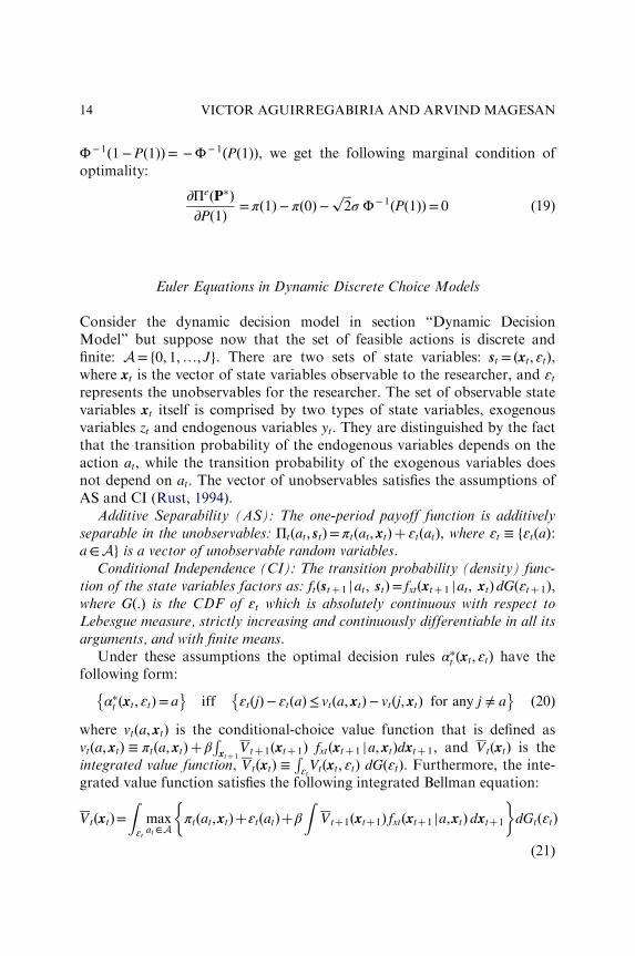
Φ− 1 1−Pð1Þð Þ= −Φ− 1 Pð1Þð Þ, we get the following marginal condition ofoptimality:

∂ΠeðP�Þ∂Pð1Þ = πð1Þ− πð0Þ−

ffiffiffi2

pσ Φ− 1 Pð1Þð Þ= 0 ð19Þ

Euler Equations in Dynamic Discrete Choice Models

Consider the dynamic decision model in section “Dynamic DecisionModel” but suppose now that the set of feasible actions is discrete andfinite: A= f0; 1;…; Jg. There are two sets of state variables: st = ðxt; ɛtÞ,where xt is the vector of state variables observable to the researcher, and ɛtrepresents the unobservables for the researcher. The set of observable statevariables xt itself is comprised by two types of state variables, exogenousvariables zt and endogenous variables yt. They are distinguished by the factthat the transition probability of the endogenous variables depends on theaction at, while the transition probability of the exogenous variables doesnot depend on at. The vector of unobservables satisfies the assumptions ofAS and CI (Rust, 1994).

Additive Separability (AS): The one-period payoff function is additivelyseparable in the unobservables: Πtðat; stÞ= πtðat; xtÞ þ ɛtðatÞ, where ɛt ≡ fɛtðaÞ:a∈Ag is a vector of unobservable random variables.

Conditional Independence (CI): The transition probability (density) func-tion of the state variables factors as: ft stþ 1 jat; stð Þ= fxt xtþ 1 jat; xtð Þ dG ɛtþ 1ð Þ,where G :ð Þ is the CDF of ɛt which is absolutely continuous with respect toLebesgue measure, strictly increasing and continuously differentiable in all itsarguments, and with finite means.

Under these assumptions the optimal decision rules α�t ðxt; ɛtÞ have thefollowing form:

α�t ðxt; ɛtÞ= a� �

iff ɛtðjÞ− ɛtðaÞ≤ vtða; xtÞ− vtðj; xtÞ for any j ≠ a� � ð20Þ

where vtða; xtÞ is the conditional-choice value function that is defined asvtða; xtÞ ≡ πtða; xtÞ þ β

Rxtþ 1

Vtþ 1ðxtþ 1Þ fxtðxtþ 1 ja; xtÞdxtþ 1, and VtðxtÞ is theintegrated value function, VtðxtÞ ≡

RɛtVtðxt; ɛtÞ dGðɛtÞ. Furthermore, the inte-

grated value function satisfies the following integrated Bellman equation:

VtðxtÞ=Zɛtmaxat∈A

πtðat;xtÞþɛtðatÞþβ

ZVtþ1ðxtþ1Þ fxtðxtþ1 ja;xtÞ dxtþ1

� �dGtðɛtÞ

ð21Þ


We can restrict our analysis to decision rules αtðxt; ɛtÞ with the following“threshold” structure: fαtðxt; ɛtÞ= ag if and only if fɛtðjÞ− ɛtðaÞ≤ μtða; xtÞ−μtðj; xtÞ for any j ≠ ag, where μtða; xtÞ is an arbitrary real valued function.As in the ARUM, we can represent decision rules using a discrete valuedfunction αtðxt; ɛtÞ, a real valued function μtða; xtÞ, or a probability valuedfunction Ptða jxtÞ.

PtðajxtÞ ≡Z

1 αtðxt; ɛtÞ= a� �

GtðɛtÞ dɛt= ~Ga μtða; xtÞ− μtðj; xtÞ: for any j ≠ 0; a

� ð22Þ

where ~Ga has the same interpretation as in the ARUM, that is, the CDF ofthe vector fɛðjÞ− ɛðaÞ : for any j ≠ ag. Lemmas 1 and 2 from the ARUMextend to this DDC model (Proposition 1 in Hotz & Miller, 1993). In parti-cular, at every period t, there is a one-to-one relationship between thevector of value differences ~μtðxtÞ ≡ fμtða; xtÞ− μtð0; xtÞ: a> 0 and the vectorof CCPs PtðxtÞ ≡ fPtðajxtÞ : a ≠ 0. We represent this mapping as PtðxtÞ=~Gð~μtðxtÞÞ, and the corresponding inverse mapping as ~μtðxtÞ= ~G

− 1ðPtðxtÞÞ.Given an arbitrary sequence of decision rules, represented in terms of

either α ≡ fαtð:Þ : t≥ 1g, or ~μ ≡ f~μtð:Þ : t≥ 1g, or P≡ fPtð:Þ : t≥ 1g, let Wet ðxtÞ

be the expected intertemporal payoff function at period t before the realiza-tion of the vector ɛt if the agent behaves according to this arbitrarysequence of decision rules. By definition

Wet xtð Þ≡E

XT − t

r=0

βr πtþ r αtþ rðxtþ r;ɛtþ rÞ;xtþ rð Þþɛtþ r αtþ rðxtþ r;ɛtþ rÞð Þ½ � j xt !

=E πt αtðxt;ɛtÞ;xtð Þþɛt αtðxt;ɛtÞð Þþβ

ZWe

tþ1 xtþ1ð Þ fxtðxtþ1jαtðxt;ɛtÞ;xtÞdxtþ1

� �ð23Þ

We denote Wet xtð Þ as the valuation function to distinguish it from the

optimal value function and to emphasize that Wet xtð Þ provides the valuation

of any arbitrary decision rule. We are interested in the representation ofthis valuation function as a function of CCPs. Therefore, we use the nota-tion We

t xt;Pt;Pt0 > tð Þ. Given its definition, this function can be written usingthe recursive formula:

Wet xt;Pt;Pt0 > tð Þ=Πe

t ðxt;PtÞ þ β

ZWe

tþ 1 xtþ 1;Ptþ 1;Pt0 > tþ 1ð Þ

× f et ðytþ 1jxt;PtÞ fzðztþ 1 jztÞdxtþ 1 ð24Þ


where Πet ðxt;PtÞ is the expected one-period profit

PJa= 0 Ptða jxtÞ½πt a; xtð Þ þ

etða;PtðxtÞÞ�; etða;PtðxtÞÞ has the same definition as in the static model, thatis, it is the expected value of ɛtðaÞ conditional on alternative a being chosenunder decision rule αtðxt; ɛtÞ10; and f et ðytþ 1jxt;PtÞ is the transition probabil-ity of the endogenous state variables y induced by the CCP function PtðxtÞ,that is,

PJa= 0 PtðajxtÞ fytðytþ 1ja; xtÞ.

The valuation function Wet xt;Pt;Pt0 > tð Þ is continuously differentiable

with respect to the choice probabilities over the simplex. Then, we candefine P� as the sequence of CCP functions fP�

t ðxÞ : t≥ 1, x∈Xg such thatfor any ðt; xÞ the vector of CCPs P�

t ðxÞ maximizes the values Wet x;Pt;Pt0 > tð Þ

given that future CCPs Pt0 > t are fixed at their values in P�.

P�t ðxÞ= arg max

PtðxÞ∈SWe

t x;Pt;P�t0 > t

� � � ð25Þ

As in the ARUM, we have apparently two different optimal CCP func-tions. We have the CCP functions associated with the sequence of optimaldecision rules α�t ð:Þ, that we represent as fPα�

t : t≥ 1g. And we have sequenceof CCP functions fP�

t : t≥ 1g defined in Eq. (25). Proposition 2 establishesthat the two sequences of CCPs are the same one, and that these probabil-ities satisfy the marginal conditions of optimality associated to the continu-ous optimization problem in Eq. (25).

Proposition 2. Let fPα�t : t≥ 1g be the sequence of CCP functions asso-

ciated with the sequence of optimal decision rules fα�t : t≥ 1g as definedin the DDC problem (20), and let fP�

t : t≥ 1g be sequence of CCP func-tions that solves the continuous optimization problem (25). Then, forevery ðt; xÞ: (i) the vectors Pα�

t ðxÞ and P�t ðxÞ are the same; and (ii) P�

t ðxÞsatisfies the marginal conditions of optimality

∂Wet x;P�

t ;P�t0 > t

� ∂PtðajxÞ

= 0 ð26Þ

for any a > 0, and the marginal value ∂Wt=∂Pt has the following form:

∂Wet

∂PtðajxÞ= vtða; xt;Pt0 > tÞ− vtð0;xt;Pt0 > tÞ þ etða;PtðxÞÞ− etð0;PtðxÞÞ

þXJj= 0

PtðjjxÞ∂etðj;PtðxÞÞ∂PtðajxÞ

ð27Þ


where vtða; xt;Pt0 > tÞ is the conditional-choice value function πtða; xtÞ þβRWtþ 1 xtþ 1;Ptþ 1;Pt0 > tþ 1ð Þ ftðxtþ 1ja; xtÞ dxtþ 1.Proof in the appendix.Proposition 2 shows that we can treat the DDC model as a dynamic

continuous optimization problem where optimal choices, in the form ofchoice probabilities, satisfy marginal conditions of optimality.Nevertheless, the marginal conditions of optimality in Eq. (27) involvevalue functions. We are looking for conditions of optimality in the spiritof Euler equations that involve only payoff functions at two consecutiveperiods, t and tþ 1. To obtain these conditions, we construct a con-strained optimization problem similar to the one for the derivation ofEuler equations in section “Euler Equations in Dynamic ContinuousDecision Models”.

By Bellman’s principle, the optimal choice probabilities at periods t andtþ 1 come from the solution to the optimization problem maxPt ;Ptþ 1

×We

t ðx;Pt;Ptþ 1;P�t0 > tþ 1Þ, where we have fixed at its optimum the individual’s

behavior at any period after tþ 1, P�t0 > tþ 1. In general, the CCPs Pt

and Ptþ 1 affect the distribution of the state variables at periods aftertþ 1 such that the optimality conditions of the problem maxPt ;Ptþ 1

×We

t ðx;Pt;Ptþ 1;P�t0 > tþ 1Þ involve payoff functions and state variables at every

period in the future. Instead, suppose that we consider a similar optimiza-tion problem but where we now impose the constraint that the probabilitydistribution of the endogenous state variables at tþ 2 should be the oneimplied by the optimal CCPs at periods t and tþ 1. Since ðP�

t ;P�tþ 1Þ satisfy

this constraint, it is clear that these CCPs represent also the unique solutionto this constrained optimization problem. That is

fP�t ðxÞ;P�

tþ1g=arg maxfPtðxÞ;Ptþ1g

Δt= Wet ðx;Pt;Ptþ1;P

�t0>tþ1Þ−We

t ðx;P�t ;P

�tþ1;P

�t0>tþ1Þ

� �subject to: f et→tþ2ð:jx;Pt;Ptþ1Þ=f et→tþ2ð:jx;P�

t ;P�tþ1Þ ð28Þ

where we use function f et→ tþ 2ð:jx;Pt;Ptþ 1Þ to represent the distribution ofytþ 2 conditional on xt = x and induced by the CCPs PtðxÞ and Ptþ 1, thatcan be written as

ft→ tþ2ðytþ2jxt;Pt;Ptþ1Þ=Z

f etþ1ðytþ2 jxtþ1;Ptþ1Þ f et ðytþ1 jxt;PtÞ fzðztþ1 jztÞdxtþ1

ð29Þ


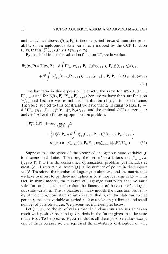
and, as defined above, f et ð:jx;PtÞ is the one-period-forward transition prob-ability of the endogenous state variables y induced by the CCP functionPtðxÞ, that is,

PJa= 0 PtðajxtÞ ftðytþ 1ja; xtÞ.

By the definition of the valuation function Wet , we have that

Wet xt;Pð Þ=Πe

t ðxt;PtÞþβ

ZΠe

tþ1 xtþ1;Ptþ1ð Þ f et ðytþ1jxt;PtÞ fzðztþ1jztÞdxtþ1

þβ2Z

Wetþ2 xtþ2;Pt0 > tþ1ð Þ ft→ tþ2ðytþ2 jxt;Pt;Ptþ1Þ fzðztþ2jztÞdxtþ2

ð30ÞThe last term in this expression is exactly the same for We

t ðx;Pt;Ptþ 1;P�t0 > tþ 1Þ and for We

t ðx;P�t ;P

�tþ 1;P

�t0 > tþ 1Þ because we have the same function

Wetþ 2 and because we restrict the distribution of ytþ 2 to be the same.

Therefore, subject to this constraint we have that Δt is equal to Πet ðx;PtÞ þ

βRΠe

tþ 1ðxtþ 1;Ptþ 1Þ f et ðxtþ 1jx;PtÞdxtþ 1, and the optimal CCPs at periods t

and tþ 1 solve the following optimization problem:

fP�t ðxÞ;P�

tþ1g=arg maxfPtðxÞ;Ptþ1g

Δt

= Πet ðx;PtÞþβ

ZΠe

tþ1ðxtþ1;Ptþ1Þ f et ðxtþ1jx;PtÞdxtþ1

� �subject to : f et→tþ2ð:jx;Pt;Ptþ1Þ=f et→tþ2ð:jx;P�

t ;P�tþ1Þ ð31Þ

Suppose that the space of the vector of endogenous state variables Yis discrete and finite. Therefore, the set of restrictions on f et→ tþ 2 ×ðytþ 2jx;Pt;Ptþ 1Þ in the constrained optimization problem (31) includes atmost jYj− 1 restrictions, where jYj is the number of points in the supportset Y. Therefore, the number of Lagrange multipliers, and the matrix thatwe have to invert to get these multipliers is of at most as large as jYj− 1. Infact, in many models, the number of Lagrange multipliers that we mustsolve for can be much smaller than the dimension of the vector of endogen-ous state variables. This is because in many models the transition probabil-ity of the endogenous state variable is such that, given the state variable atperiod t, the state variable at period tþ 2 can take only a limited and smallnumber of possible values. We present several examples below.

Let Y þ sðxtÞ be the set of values that the endogenous state variables canreach with positive probability s periods in the future given that the statetoday is xt. To be precise, Y þ sðxtÞ includes all these possible values exceptone of them because we can represent the probability distribution of ytþ s


using the probabilities of each possible value except one. Let λtðxtÞ=fλtðytþ 2jxtÞ : ytþ 2 ∈Y þ 2ðxtÞg be the jY þ 2ðxtÞj× 1 vector of Lagrange multi-pliers associated to this set of restrictions. The Lagrangian function for thisoptimization problem is

LtðPtðxtÞ;Ptþ1Þ=Πet ðx;PtÞþβ

Xxtþ1

Πetþ1ðxtþ1;Ptþ1Þ f et ðytþ1 j xt;PtÞ fzðztþ1jztÞ

−Xytþ2

λtðytþ2jxtÞXxtþ1

f etþ1ðytþ2jxtþ1;Ptþ1Þ f et ðytþ1 jxt;PtÞfzðztþ1jztÞ" #

ð32Þ

Given this Lagrangian function, we can derive the first order conditionsof optimality with respect to PtðxtÞ and Ptþ 1 and combine these conditionsto obtain Euler equations.

Proposition 3. The marginal conditions for the maximization of theLagrangian function in Eq. (32) imply the following Euler equations.For every value of xt:

∂Πet

∂PtðajxtÞþβXxtþ1

Πetþ1ðxtþ1Þ−mðxtþ1Þ0

∂Πetþ1ðztþ1Þ

∂Ptþ1ðztþ1Þ

� �~f tðytþ1ja;xtÞ fzðztþ1jztÞ=0

ð33Þ

where ~f tðytþ1ja;xtÞ≡ ftðytþ1ja;xtÞ− ftðytþ1j0; xtÞ; ∂Πetþ1ðztþ1Þ=∂Ptþ1ðztþ1Þ

is a column vector with dimension JjYþ1ðxtÞj×1 that contains the partialderivatives f∂Πe

tþ1ðytþ1;ztþ1Þ=∂Ptþ1ðajytþ1; ztþ1Þg for every action a>0and every value ytþ1∈Yþ1ðxtÞ that can be reach from xt, and fixed valuefor ztþ1; and mðxtþ1Þ is a JjYþ1ðxtÞj×1 vector such that mðxtþ1Þ≡fetþ1ðxtþ1Þ0½ ~Ftþ1ðztþ1Þ0 ~Ftþ1ðztþ1Þ�−1 ~Ftþ1ðztþ1Þ0 where fetþ1ðxtþ1Þ is thevector of transition probabilities ff etþ1ðytþ2jxtþ1Þ : ytþ2∈Yþ2ðxtÞg, and~Ftþ1ðztþ1Þ is matrix with dimension JjYþ1ðxtÞj× jYþ2ðxtÞj that containsthe probabilities ~f tþ1ðytþ2ja;xtþ1Þ for every ytþ2∈Yþ2ðxtÞ, every ytþ1∈Yþ1ðxtÞ, and every action a>0, with fixed ztþ1.

Proof in the appendix.Proposition 3 shows that in general we can derive marginal conditional

of optimality that involve only payoffs and states at two consecutiveperiods. The derivation of this Euler equation, described in the appendix,is based on the combination of the Lagrangian conditions ∂Lt=∂PtðajxtÞ= 0


and ∂Lt=∂Ptþ 1ðajxtþ 1Þ= 0. Using the group of conditions ∂Lt=∂Ptþ 1

ðajxtþ 1Þ= 0 we can solve for the vector of Lagrange multipliers as½ ~Ftþ 1ðztþ 1Þ0 ~Ftþ 1ðztþ 1Þ�− 1 ~Ftþ 1ðztþ 1Þ0∂Πe

tþ 1ðztþ 1Þ=∂Ptþ 1ðztþ 1Þ and then wecan plug this solution into the first Lagrangian conditions, ∂Lt=∂PtðajxtÞ= 0.This provides the expression for the Euler equation in (33). The main com-putational cost in the derivation of this expression comes from inverting thematrices ½ ~Ftþ 1ðztþ 1Þ0 ~Ftþ 1ðztþ 1Þ�. The dimension of these matrices isjY þ 2ðxtÞj× jY þ 2ðxtÞj, where Y þ 2ðxtÞ is the set of possible values that theendogenous state variable ytþ 2 can take given xt. In most applications, thenumber of elements in the set Y þ 2ðxtÞ is substantially smaller that the wholenumber of values in the space of the endogenous state variable, and severalorders of magnitude smaller than the dimension of the complete state spacethat includes the exogenous state variables. This property implies very sub-stantial computational savings in the estimation of the model. We now pro-vide some examples of models where the form of the Euler equations isparticularly simple. In these examples, we have simple closed form expres-sions for the Lagrange multipliers. These examples correspond to modelsthat are commonly estimated in applications of DDC models.

Example 4. (Dynamic binary choice model of entry and exit). Consider abinary decision model, A= f0; 1g, where at is the indicator of beingactive in a market or in some particular activity. The endogenous statevariable yt is the lagged value of the decision variable, yt = at− 1, andit represents whether the agent was active at previous period. The vectorof state variables is then xt = ðyt; ztÞ where zt are exogenous statevariables. Suppose that ɛtð0Þ and ɛtð1Þ are extreme value type 1 distri-buted with dispersion parameter σɛ. In this model, the one-periodexpected payoff function is Πe

t ðxt;PtÞ=Ptð0jxtÞ ½π 0; xtð Þ−σɛ lnPtð0jxtÞ�þPtð1jxtÞ ½π 1; xtð Þ−σɛ lnPtð1jxtÞ�. The transition of the endogenous statevariable induced by the CCP is the CCP itself, that is, f et ðytþ1jxt;PtÞ=Ptðytþ1jxtÞ. Therefore, we can write the Δt function in the constrainedoptimization problem as

Δt =Πet ðxt;PtÞ þ β

Xztþ 1

fzðztþ 1jztÞ ½Ptð0jxtÞΠetþ 1ð0;ztþ 1;Ptþ 1Þ

þPtð1jxtÞ Πetþ 1ð1;ztþ 1;Ptþ 1Þ� ð34Þ

Given xt, the state variable ytþ 2 can take two values, 0 or 1. Therefore,there is only one free probability in f et→ tþ 2 and one restriction in theLagrangian problem. This probability is


f et→ tþ 2ð1jxt;Pt;Ptþ 1Þ=Xztþ 1

fzðztþ 1jztÞ ½Ptð0jxtÞPtþ 1ð1j0; ztþ 1Þ

þPtð1jxtÞPtþ 1ð1j1; ztþ 1Þ� ð35ÞLet λðxtÞ be the Lagrange multiplier for this restriction. For a given xt,

the free probabilities that enter in the Lagrangian problem are Ptð1jxtÞ,Ptþ 1ð1j0; ztþ 1Þ, and Ptþ 1ð1j1; ztþ 1Þ for any possible value of ztþ 1 in thesupport set Z. The first order condition for the maximization of theLagrangian with respect to Ptð1jxtÞ is

∂Πet

∂Ptð1jxtÞþ β

Xztþ 1

½Πetþ 1ð1Þ−Πe

tþ 1ð0Þ− λðxtÞfPtþ 1ð1j1; ztþ 1Þ

−Ptþ 1ð1j0; ztþ 1Þg� fzðztþ 1jztÞ= 0 ð36ÞThe marginal condition with respect to one of the probabilities Ptþ 1ð1jxtþ 1Þ

(for a given value of xtþ 1) is β∂Πe

tþ 1ð0;ztþ 1;Ptþ 1Þ∂Ptþ 1ð1j0;ztþ 1Þ = β

∂Πetþ 1ð1;ztþ 1;Ptþ 1Þ∂Ptþ 1ð1j1;ztþ 1Þ = λðxtÞ.

Substituting the marginal condition with respect to Ptþ 1ð1jxtþ 1Þ into themarginal condition with respect to Ptð1jxtÞ we get the Euler equation:

∂Πet

∂Ptð1jxtÞþβEt Πe

tþ1ð1;ztþ1Þ−Πetþ1ð0;ztþ1Þ

�

þβEt Ptþ1ð1j0;ztþ1Þ∂Πe

tþ1ð0;ztþ1;Ptþ1Þ∂Ptþ1ð1j0;ztþ1Þ

−Ptþ1ð1j1;ztþ1Þ∂Πe

tþ1ð1;ztþ1;Ptþ1Þ∂Ptþ1ð1j1;ztþ1Þ

0@

1A

=0

ð37Þwhere we use Etð:Þ to represent in a compact form the expectation over thedistribution of fzðztþ 1jztÞ. Finally, for the logit version of this model and asshown in Example 2, the marginal expected profit ∂Πe

t =∂Ptð1jxtÞ is equal toπ 1; xtð Þ− πt 0; xtð Þ− σɛðlnPtð1jxtÞ− lnPtð0jxtÞÞ. Taking this into account andoperating in the Euler equation, we can obtain this simpler formula for thisEuler equation:

π 1; yt; ztð Þ− π 0; yt; ztð Þ− σɛlnPtð1jyt; ztÞPtð0jyt; ztÞ

0@

1A

24

35

þ βEt π 1; 1; ztþ 1ð Þ− πt 1; 0; ztþ 1ð Þ− σɛ lnPtþ 1ð1j1; ztþ 1ÞPtþ 1ð1j0; ztþ 1Þ

0@

1A

24

35= 0

ð38Þ


Example 5. (Machine replacement model). Consider a model where thebinary choice variable at is the indicator for a firm’s decision to replacean old machine or equipment by a new one. The endogenous state vari-able yt is the age of the “old” machine that takes discrete values f1; 2;…gand it follows the transition rule ytþ 1 = 1þð1− atÞyt, that is, if the firmreplaces the machine at period t (i.e., at = 1), then at period tþ 1 it has abrand new machine with ytþ 1 = 1, otherwise the firm continues with theold machine that at tþ 1 will be one period older. Given yt, we have thatytþ 1 can take only two values, ytþ 1 ∈ f1; yt þ 1g. Thus, the Δt function is

Δt =Πet ðxtÞ þ β

Xztþ 1

fzðztþ 1jztÞ½Ptð0jxtÞΠetþ 1ðyt þ 1; ztþ 1Þ

þPtð1jxtÞΠetþ 1ð1; ztþ 1Þ� ð39Þ

Given yt, we have that ytþ 2 can take only three values, ytþ 1 ∈f1; 2; yt þ 1g. There are only two free probabilities in the distribution off et→ tþ 2ðytþ 2jxtÞ. Without loss of generality, we use the probabilitiesf et→ tþ 2ð1jxtÞ and f et→ tþ 2ð2jxtÞ to construct the Lagrange function. Theseprobabilities have the following form:

f et→ tþ 2ð1jxtÞ=Xztþ 1

fzðztþ 1jztÞ½Ptð0jxtÞPtþ 1ð1jyt þ 1; ztþ 1Þ

þPtð1jxtÞPtþ 1ð1j1; ztþ 1Þ�f et→ tþ 2ð2jxtÞ=Ptð1jxtÞ

Xztþ 1

fzðztþ 1jztÞPtþ 1ð0j1; ztþ 1Þ ð40Þ

The Lagrangian function depends on the CCPs Ptð1jxtÞ, Ptþ 1ð1j1; ztþ 1Þ,and Ptþ 1ð1jyt þ 1; ztþ 1Þ. The Lagrangian optimality condition with respectto Ptð1jxtÞ is

∂Πet

∂Ptð1jxtÞþ β

Xztþ 1

fzðztþ 1jztÞ Πetþ 1ð1; ztþ 1Þ−Πe

tþ 1ðyt þ 1; ztþ 1Þ� �

− λð1ÞXztþ 1

fzðztþ 1jztÞ Ptþ 1ð1j1; ztþ 1Þ−Ptþ 1ð1jyt þ 1; ztþ 1Þ½ �

− λð2ÞXztþ 1

fzðztþ 1jztÞPtþ 1ð0j1; ztþ 1Þ= 0

ð41ÞAnd the Lagrangian conditions with respect to Ptþ 1ð1j1; ztþ 1Þ and

Ptþ 1ð1jyt þ 1; ztþ 1Þ are β ∂Πetþ 1ð1;ztþ 1Þ

∂Ptþ 1ð1j1;ztþ 1Þ − λð1Þ þ λð2Þ= 0, and β∂Πe

tþ 1ðyt þ 1;ztþ 1Þ∂Ptþ 1ð1jyt þ 1;ztþ 1Þ −


λð1Þ= 0, respectively. We can use the second set of conditions to solvetrivially for the Lagrange multipliers, and then plug in the expression forthis multipliers in the first set of Lagrangian conditions. We obtain theEuler equation:

∂Πet

∂Ptð1jxtÞþβEt Πe

tþ1ð1; ztþ1Þ−Πetþ1ðytþ1; ztþ1Þ

� �

þβEt

∂Πetþ1ð1; ztþ1Þ

∂Ptþ1ð1j1; z tþ1ÞPtþ1ð0j1; ztþ1Þ−∂Πe

tþ1ðytþ1; ztþ1Þ∂Ptþ1ð1jytþ1; ztþ1Þ

Ptþ1ð0jytþ1; ztþ1Þ24

35=0ð42Þ

Finally, taking into account that for the logit specification of theunobservables the marginal expected profit ∂Πe

t =∂Ptð1jxtÞ is equal toπ 1; xtð Þ− π 0; xtð Þ− σɛ½ln Ptð1jxtÞ− ln Ptð0jxtÞ�, and operating in the previousexpression, it is possible to obtain the following Euler equation:

π 1; yt; ztð Þ− π 0; yt; ztð Þ− σɛ lnPtð1jyt; ztÞPtð0jyt; ztÞ

0@

1A

24

35

þ β Et π 1; 1; ztþ 1ð Þ− π 1; yt þ 1; ztþ 1ð Þ− σɛ lnPtþ 1ð1j1; ztþ 1Þ

Ptþ 1ð1jyt þ 1; ztþ 1Þ

0@

1A

24

35= 0

ð43Þ

Relationship between Euler Equations and Other CCP Representations

Our derivation of Euler equations for DDC models above is related toprevious work by Hotz and Miller (1993), Aguirregabiria and Mira (2002),and Arcidiacono and Miller (2011). These papers derive representations ofoptimal decision rules using CCPs and show how these representations canbe applied to estimate DDC models using simple two-step methods thatprovide substantial computational savings relative to full-solution methods.In these previous papers, we can distinguish three different types ofCCP representations of optimal decisions rules: (1) the present-value repre-sentation; (2) the terminal-state representation; and (3) the finite-dependencerepresentation.

The present-value representation consists of using CCPs to obtain anexpression for the expected and discounted stream of future payoffs asso-ciated with each choice alternative. In general, given CCPs, the valuation


function Wet x;Pð Þ can be obtained recursively using its definition,

Wet xt;Pð Þ=Πe

t ðxt;PÞ þ βRWe

tþ 1 xtþ 1;Pð Þ f et ðxtþ 1jxt;PÞ dxtþ 1. And given thisvaluation function we can construct the agent’s optimal decision rule (orbest response) at period t given that he believes that in the future he willbehave according to the CCPs in the vector P. This present-value represen-tation is the CCP approach more commonly used in empirical applicationsbecause it can be applied to a general class of DDC models. However, thisrepresentation requires the computation of present values and therefore itis subject to the curse of dimensionality. In applications with large statespaces, this approach can be implemented only if it is combined with anapproximation method such as the discretization of the state space, orMonte Carlo simulation (e.g., Bajari et al., 2007; Hotz et al., 1994). In gen-eral, these approximation methods introduce a bias in parameter estimates.

The terminal-state representation was introduced by Hotz and Miller(1993) and it applies only to optimal stopping problems with a terminalstate. The finite-dependence representation was introduced by Arcidiaconoand Miller (2011) and applies to a particular class of DDC models with thefinite dependence property. A DDC model has the finite dependence prop-erty if given two values of the decision variable at period t and their respec-tive paths of the state variables after this period, there is always a finiteperiod t0 > t (with probability one) where the state variables in the two pathstake the same value. The terminal-state and the finite-dependence CCP repre-sentations do not involve the computation of present values, or even theestimation of CCPs at every possible state. This implies substantial compu-tational savings as well as avoiding biases induced by approximation errors.

The system of Euler equations that we have derived in Proposition 3 canbe seen also as a CCP representation of the optimal decision rule in a DDCmodel. Our representation shares all the computational advantages of theterminal-state and finite-dependence representations. However, in contrastto the terminal-state and finite-dependence, our Euler equation representa-tion applies to a general class of DDC models. We can derive Euler equa-tions for any DDC model where the unobservables satisfy the conditions ofAS in the payoff function, and CI in the transition of the state variables.

GMM ESTIMATION OF EULER EQUATIONS

Suppose that the researcher has panel data of N agents over ~T periods oftime, where he observes agents’ actions fait : i= 1; 2; …; N; t= 1; 2; …; ~Tg,


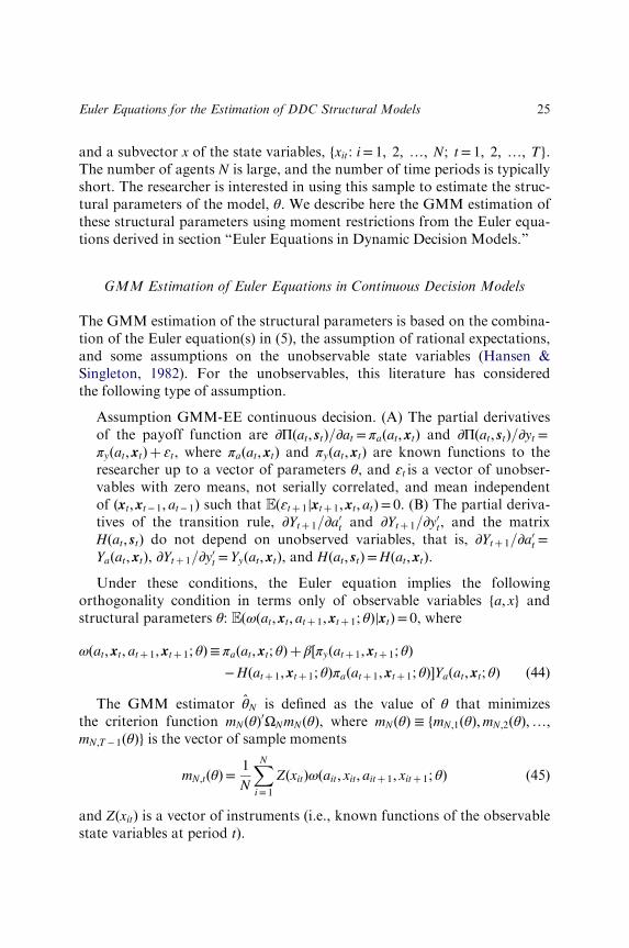
and a subvector x of the state variables, fxit : i= 1; 2; …; N; t= 1; 2; …; Tg.The number of agents N is large, and the number of time periods is typicallyshort. The researcher is interested in using this sample to estimate the struc-tural parameters of the model, θ. We describe here the GMM estimation ofthese structural parameters using moment restrictions from the Euler equa-tions derived in section “Euler Equations in Dynamic Decision Models.”

GMM Estimation of Euler Equations in Continuous Decision Models

The GMM estimation of the structural parameters is based on the combina-tion of the Euler equation(s) in (5), the assumption of rational expectations,and some assumptions on the unobservable state variables (Hansen &Singleton, 1982). For the unobservables, this literature has consideredthe following type of assumption.

Assumption GMM-EE continuous decision. (A) The partial derivativesof the payoff function are ∂Πðat; stÞ=∂at = πaðat; xtÞ and ∂Πðat; stÞ=∂yt =πyðat; xtÞ þ ɛt, where πaðat; xtÞ and πyðat; xtÞ are known functions to theresearcher up to a vector of parameters θ, and ɛt is a vector of unobser-vables with zero means, not serially correlated, and mean independentof ðxt; xt− 1; at− 1Þ such that Eðɛtþ 1jxtþ 1; xt; atÞ= 0. (B) The partial deriva-tives of the transition rule, ∂Ytþ 1=∂a0t and ∂Ytþ 1=∂y0t, and the matrixHðat; stÞ do not depend on unobserved variables, that is, ∂Ytþ 1=∂a0t =Yaðat; xtÞ, ∂Ytþ 1=∂y0t = Yyðat; xtÞ, and Hðat; stÞ=Hðat; xtÞ.Under these conditions, the Euler equation implies the following

orthogonality condition in terms only of observable variables fa; xg andstructural parameters θ: Eðωðat; xt; atþ 1; xtþ 1; θÞjxtÞ= 0, where

ωðat; xt; atþ 1; xtþ 1; θÞ≡ πaðat; xt; θÞ þ β½πyðatþ 1; xtþ 1; θÞ−Hðatþ 1; xtþ 1; θÞπaðatþ 1; xtþ 1; θÞ�Yaðat; xt; θÞ ð44Þ

The GMM estimator θ̂N is defined as the value of θ that minimizesthe criterion function mNðθÞ0ΩNmNðθÞ, where mNðθÞ ≡ fmN;1ðθÞ;mN;2ðθÞ;…;mN;T − 1ðθÞg is the vector of sample moments

mN;tðθÞ= 1

N

XNi= 1

ZðxitÞωðait; xit; aitþ 1; xitþ 1; θÞ ð45Þ

and ZðxitÞ is a vector of instruments (i.e., known functions of the observablestate variables at period t).


The GMM-Euler equation approach for dynamic models with continuousdecision variables has been extended to models with corner solutions andcensored decision variables (Aguirregabiria, 1997; Cooper, Haltiwanger, &Willis, 2010; Pakes, 1994), and to dynamic games (Berry & Pakes, 2000).11

GMM Estimation of Static Random Utility Models

Consider the ARUM in section “Random Utility Model as a ContinuousOptimization Problem.” Now, the deterministic component of the utilityfunction for agent i is πðai; xi; θÞ, where xi is a vector of exogenous charac-teristics of agent i and of the environment which are observable to theresearcher, and θ is a vector of structural parameters. Given a randomsample of N individuals with information on fai; xig, the marginal condi-tions of optimality in Eq. (16) can be used to construct a semiparametrictwo-step GMM estimator of the structural parameters. The first step con-sists in the nonparametric estimation of the CCPs PðajxÞ ≡ Prðait = ajxit = xÞ.Let P̂N ≡ fP̂ðajxiÞg be a vector of nonparametric estimates of CCPs for anychoice alternative a and any value of xi in the sample. For instance, P̂tðajxÞcan be a kernel (Nadaraya�Watson) estimator of the regression between1fai = ag and xi. In the second step, the vector of parameters θ is estimatedusing the following GMM estimator:

θ̂N = argminθ∈Θ

m0N θ; P̂N

� ΩNmN θ; P̂N

� ð46Þ

where mNðθ;PÞ ≡ fmN;1ðθ;PÞ;mN;2ðθ;PÞ ;…; mN;Jðθ;PÞg is the vector of sam-ple moments, with

mN;aðθ;PÞ= 1

N

XNi= 1

Zi πða; xi; θÞ− πð0; xi; θÞ þ eða; xi;PÞ"

− eð0; xi;PÞ þXJj= 0

PðjjxiÞ∂eðj; xi;PÞ∂PðajxiÞ

#ð47Þ

This two-step semiparametric estimator is root-N consistent and asymp-totically normal under mild regularity conditions (see Theorems 8.1 and 8.2in Newey & McFadden, 1994). The variance matrix of this estimator canbe estimated using the semiparametric method in Newey (1994), or as


recently shown by Ackerberg, Chen, and Hahn (2012) using a computa-tionally simpler parametric-like method as in Newey (1984).

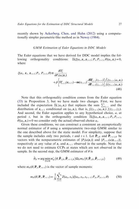
GMM Estimation of Euler Equations in DDC Models

The Euler equations that we have derived for DDC model implies the fol-lowing orthogonality conditions: Eðξðat; xt; xtþ 1;Pt;Ptþ 1; θÞjat; xtÞ= 0,where

ξðat; xt; xtþ1;Pt; Ptþ1;θÞ≡∂Πe

t

∂PtðatjxtÞ

þβ Πetþ1ðxtþ1Þ−mðxtþ1Þ0

∂Πetþ1ðztþ1Þ

∂Ptþ1ðztþ1Þ

� � ~f tðytþ1jat;xtÞftðytþ1jat;xtÞ

ð48Þ

Note that this orthogonality condition comes from the Euler equation(33) in Proposition 3, but we have made two changes. First, we haveincluded the expectation Eð:jat; xtÞ that replaces the sum

Pxtþ 1

and thedistribution of xtþ 1 conditional on ðat; xtÞ, that is, ftðytþ 1jat; xtÞ fzðztþ 1jztÞ.And second, the Euler equation applies to any hypothetical choice, a, atperiod t, but in the orthogonality condition Eðξðat; xt; xtþ 1;Pt;Ptþ 1;θÞjat; xtÞ= 0 we consider only the actual/observed choice at.

Given these conditions, we can construct a consistent an asymptoticallynormal estimator of θ using a semiparametric two-step GMM similar tothe one described above for the static model. For simplicity, suppose thatthe sample includes only two periods, t and tþ 1. Let P̂t;N and P̂tþ 1;N bevectors with the nonparametric estimates of fPtðajxtÞg and fPtþ 1ðajxtþ 1Þg,respectively at any value of xt and xtþ 1 observed in the sample. Note thatwe do not need to estimate CCPs at states which are not observed in thesample. In the second step, the GMM estimator of θ is

θ̂N = argminθ∈Θ

m0N θ; P̂t;N ; P̂tþ 1;N

� ΩNmN θ; P̂t;N ; P̂tþ 1;N

� ð49Þ

where mNðθ;Pt;Ptþ 1Þ is the vector of sample moments:

mNðθ;Pt;Ptþ 1Þ=1

N

XNi= 1

Zðait; xitÞξðait; xit; xitþ 1;Pit;Pitþ 1; θÞ ð50Þ


Zðait; xitÞ is a vector of instruments, that is, known functions of theobservable decision and state variables at period t. As in the case of the sta-tic ARUM, this semiparametric two-step GMM estimator is consistent andasymptotically normal under mild regularity conditions.

Relationship with Other CCP Estimators

The estimation based on the moment conditions provided by the Eulerequation, or terminal-state, or finite-dependence representations imply anefficiency loss relative to estimation based on present-value representation.As shown by Aguirregabiria and Mira (2002, Proposition 4), the two-stepPML estimator based on the CCP present-value representation is asympto-tically efficient (equivalent to the ML estimator). This efficiency property isnot shared by the other CCP representations. Therefore, there is a trade-offin the choice between CCP estimators based on Euler equations and onpresent-value representations. The present-value representation is the bestchoice in models that do not require approximation methods. However, inmodels with large state spaces that require approximation methods, theEuler equations CCP estimator can provide more accurate estimates.

AN APPLICATION

This section presents an application of the Euler equations-GMM methodto a binary choice model of firm investment. More specifically, we considerthe problem of a dairy farmer who has to decide when to replace a dairycow by a new heifer. The cow replacement model that we consider here isan example of asset or “machine” replacement model.12 We estimate thismodel using data on dairy cow replacement decisions and milk productionusing a two-step PML estimator and the ML estimator, and compare theseestimates to those of the Euler equations-GMM method.

Model

Consider a farmer that produces and sells milk using dairy cows. The farmcan be conceptualized as a plant with a fixed number of stalls n, one foreach dairy cow. We index time by t and stalls by i. In our model, one


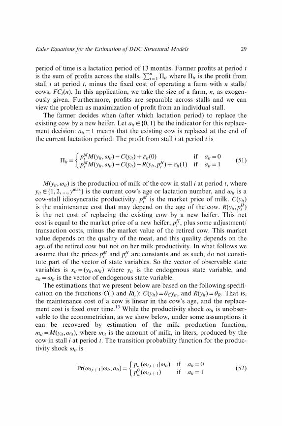
period of time is a lactation period of 13 months. Farmer profits at period t

is the sum of profits across the stalls,Pn

i= 1 Πit where Πit is the profit fromstall i at period t, minus the fixed cost of operating a farm with n stalls/cows, FCtðnÞ. In this application, we take the size of a farm, n, as exogen-ously given. Furthermore, profits are separable across stalls and we canview the problem as maximization of profit from an individual stall.

The farmer decides when (after which lactation period) to replace theexisting cow by a new heifer. Let ait ∈ f0; 1g be the indicator for this replace-ment decision: ait = 1 means that the existing cow is replaced at the end ofthe current lactation period. The profit from stall i at period t is

Πit =pMt Mðyit;ωitÞ−CðyitÞ þ ɛitð0Þ if ait = 0

pMt Mðyit;ωitÞ−CðyitÞ−Rðyit; pHt Þþ ɛitð1Þ if ait = 1

�ð51Þ

Mðyit;ωitÞ is the production of milk of the cow in stall i at period t, whereyit ∈ f1; 2; :::; ymaxg is the current cow’s age or lactation number, and ωit is acow-stall idiosyncratic productivity. pMt is the market price of milk. CðyitÞis the maintenance cost that may depend on the age of the cow. Rðyit; pHt Þis the net cost of replacing the existing cow by a new heifer. This netcost is equal to the market price of a new heifer, pHt , plus some adjustment/transaction costs, minus the market value of the retired cow. This marketvalue depends on the quality of the meat, and this quality depends on theage of the retired cow but not on her milk productivity. In what follows weassume that the prices pMt and pHt are constants and as such, do not consti-tute part of the vector of state variables. So the vector of observable statevariables is xit = ðyit;ωitÞ where yit is the endogenous state variable, andzit =ωit is the vector of endogenous state variable.

The estimations that we present below are based on the following specifi-cation on the functions Cð:Þ and Rð:Þ: CðyitÞ= θCyit, and RðyitÞ= θR. That is,the maintenance cost of a cow is linear in the cow’s age, and the replace-ment cost is fixed over time.13 While the productivity shock ωit is unobser-vable to the econometrician, as we show below, under some assumptions itcan be recovered by estimation of the milk production function,mit =Mðyit;ωitÞ, where mit is the amount of milk, in liters, produced by thecow in stall i at period t. The transition probability function for the produc-tivity shock ωit is

Prðωi;tþ 1jωit; aitÞ= pωðωi;tþ 1jωitÞ if ait = 0

p0ωðωi;tþ 1Þ if ait = 1

�ð52Þ


An important feature of this transition probability is that the productivityof a new heifer is independent of the productivity of the retired cow. Oncewe have recovered ωit, the transition function for the productivity shockcan be identified from the data. The transition rule for the cow age is tri-vial: yi;tþ 1 = 1þ ð1− aitÞyit. The unobservables ɛitð0Þ and ɛitð1Þ are assumedi.i.d. over i and over t with type 1 extreme value distribution with disper-sion parameter σɛ.

Data

The dataset comes from Miranda and Schnitkey (1995). It contains infor-mation on the replacement decision, age and milk production of cows fromfive Ohio dairy farms over the period 1986�1992. There are 2,340 observa-tions from a total of 1,103 cows: 103 cows from farmer 1; 187 cows fromfarmer 2; 365 from farmer 3; 282 from farmer 4; and 166 cows from thelast farmer. The data were provided by these five farmers through theDairy Herd Improvement Association.

Here we use the sample of cows which entered in the production processbefore 1987. The reason for this selection is that for these initial cohorts wehave complete lifetime histories for every cow, while for the later cohortswe have censored durations. Our working sample consists of 357 cows and783 observations.

Table 1. Descriptive Statistics (Working Sample: 357 Cows withComplete Spells).

Cow Lactation Period (Age)

1 2 3 4 5

Distribution of cows (%) by

age of replacement

113 126 68 37 13

(31.7%) (35.3%) (19.0%) (10.4%) (3.6%)

Hazard rate for the

replacement decision

0.317 0.516 0.571 0.740 1.000

Mean Milk Production

(thousand pounds) by age

(row) and age at replacement

(column)

1 14.90 18.13 18.76 18.42 16.85

2 � 17.42 19.80 20.46 19.40

3 � � 20.06 23.74 22.28

4 � � � 20.07 21.60

5 � � � � 16.99


In Table 1 we provide some basic descriptive statistics from our workingsample. The hazard rate for the replacement decision increases monotoni-cally with the age of the cow. Average milk production (per cow and per-iod) presents an inverted-U shape pattern both with respect to the currentage of the cow and with respect to the age of the cow at the moment ofreplacement. This evidence is consistent with a causal effect of age of milkoutput but also with a selection effect, that is, more productive cows tendto be replaced at older ages.

Estimation

In this section we estimate the structural parameters of the profit functionusing our Euler equations method, as well as two more standard methodsfor estimation of DDC models, the two-step PML method and ML methodfor illustrative purposes.

Estimation of Milk Production FunctionRegardless of the method we use to estimate the structural parametersin the cost functions, we first estimate the milk production function,mit =Mðyit;ωitÞ, outside the dynamic programming problem. We consider aspecification for milk production that is nonparametric in age, and log-additive in the productivity shock ωit:

ln ðmitÞ=Xymax

j= 1

αj1fyit = jgþωit ð53Þ

A potentially important issue in the estimation of this production func-tion is that we expect age yit to be positively correlated with the productiv-ity shock ωit. Less productive cows are replaced at early ages, and highproductivity cows at later ages. Therefore, OLS estimates of α will not havea causal interpretation, as the age of the cow yit is positively correlated withunobserved productivity ωit. Specifically, we would expect that E½ωitjyit� isincreasing in yit as more productive cows survive longer than less produc-tive ones. This would tend to bias downward the α0s at early ages andupward bias the α0s at old ages.14

To overcome this endogeneity problem, we consider the followingapproach. First, note that if the productivity shock were not serially corre-lated, there would be no endogeneity problem because age is a


predetermined variable which is not correlated with an unanticipated shockat period t. Therefore, if we can transform the production function suchthat the unobservable is not serially correlated, then the unobservable inthe production function will not be correlated with age. Note that the pro-ductivity shock ωit is cow specific and is not transferred to another cow inthe same stall. Therefore, if the age of the cow is 1, we have that ωit is notcorrelated with 1fyit = 1g. That is,

α1 =E lnðmitÞjyit = 1½ � ð54Þ

and we can estimate consistently α1 using the frequency estimator½Pi;t1fyit = 1g ln ðmitÞ�=½

Pi;t1fyit = 1g�. For ages greater than 1, we assume

that ωit follows an AR(1) process, ωit = ρ ωit− 1 þ ξit, where ξit is an i.i.d.shock. Then, we can transform the production function to obtain thefollowing sequence of equations. For yit ≥ 2

lnðmitÞ= ρ ln ðmit− 1Þ þXyHj= 2

γj1fyit = jgþ ξit ð55Þ

where γj ≡ αj − ρ αj− 1. OLS estimation of this equation provides consistentestimates of ρ and γ0s. Finally, using these estimates and the estimator ofα1, we obtain consistent estimates of ρ and α0s. We can also iterate in thisprocedure to obtain Cochrane�Orcutt FGLS estimator.

Table 2. Estimation of Milk Production Function (Working Sample: 357Cows with Complete Spells).

Explanatory Variables Estimates (Standard Errors)

Not controlling for

selection

Controlling for

selection

γ parameters α parameters

lnðmit− 1Þ � 0.636 (0.048)

1fAge= 1g 2.823 (0.011) � 2.823 (0.010)

1fAge= 2g 2.905 (0.014) 1.068 (0.139) 2.863 (0.014)

1fAge= 3g 3.047 (0.019) 1.150 (0.144) 2.971 (0.020)

1fAge= 4g 3.001 (0.030) 1.004 (0.152) 2.894 (0.030)

1fAge= 5g 2.809 (0.059) 0.862 (0.155) 2.702 (0.057)

R2 0.13 0.364

Number of observations 783 426


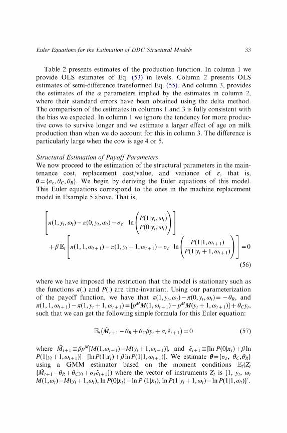
Table 2 presents estimates of the production function. In column 1 weprovide OLS estimates of Eq. (53) in levels. Column 2 presents OLSestimates of semi-difference transformed Eq. (55). And column 3, providesthe estimates of the α parameters implied by the estimates in column 2,where their standard errors have been obtained using the delta method.The comparison of the estimates in columns 1 and 3 is fully consistent withthe bias we expected. In column 1 we ignore the tendency for more produc-tive cows to survive longer and we estimate a larger effect of age on milkproduction than when we do account for this in column 3. The difference isparticularly large when the cow is age 4 or 5.

Structural Estimation of Payoff ParametersWe now proceed to the estimation of the structural parameters in the main-tenance cost, replacement cost/value, and variance of ɛ, that is,θ= fσɛ ; θC; θRg. We begin by deriving the Euler equations of this model.This Euler equations correspond to the ones in the machine replacementmodel in Example 5 above. That is,

π 1; yt;ωtð Þ− π 0; yt;ωtð Þ− σɛ lnPð1jyt;ωtÞPð0jyt;ωtÞ

0@

1A

24

35

þ βEt π 1; 1;ωtþ 1ð Þ− π 1; yt þ 1;ωtþ 1ð Þ− σɛ lnPð1j1;ωtþ 1Þ

Pð1jyt þ 1;ωtþ 1Þ

0@

1A

24

35= 0

ð56Þ

where we have imposed the restriction that the model is stationary such asthe functions πð:Þ and Pð:Þ are time-invariant. Using our parameterizationof the payoff function, we have that π 1; yt;ωtð Þ− π 0; yt;ωtð Þ= − θR, andπ 1; 1;ωtþ 1ð Þ− π 1; yt þ 1;ωtþ 1ð Þ= ½pMMð1;ωtþ 1Þ− pMMðyt þ 1;ωtþ 1Þ� þ θCyt,such that we can get the following simple formula for this Euler equation:

Et~Mtþ 1 − θR þ θCβyt þ σɛ ~etþ 1

� = 0 ð57Þ

where ~Mtþ1≡βpM½Mð1;ωtþ1Þ−Mðytþ1;ωtþ1Þ�, and ~etþ1≡ ½ln Pð0jxtÞþβ lnPð1jytþ1;ωtþ1Þ�− ½lnPð1jxtÞþβ lnPð1j1;ωtþ1Þ�. We estimate θ=fσɛ; θC;θRgusing a GMM estimator based on the moment conditions EtðZtf ~Mtþ1−θRþθCytþσɛ ~etþ1gÞ where the vector of instruments Zt is f1, yt, ωt

Mð1;ωtÞ−Mðytþ1;ωtÞ, ln Pð0jxtÞ− ln P ð1jxtÞ, ln Pð1jytþ1;ωtÞ− ln Pð1j1;ωtÞg0.


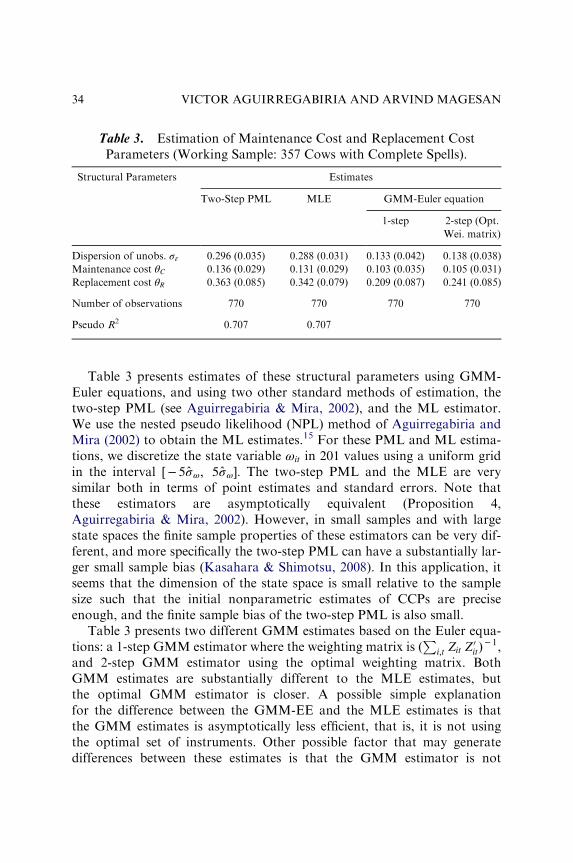
Table 3 presents estimates of these structural parameters using GMM-Euler equations, and using two other standard methods of estimation, thetwo-step PML (see Aguirregabiria & Mira, 2002), and the ML estimator.We use the nested pseudo likelihood (NPL) method of Aguirregabiria andMira (2002) to obtain the ML estimates.15 For these PML and ML estima-tions, we discretize the state variable ωit in 201 values using a uniform gridin the interval ½− 5σ̂ω; 5σ̂ω�: The two-step PML and the MLE are verysimilar both in terms of point estimates and standard errors. Note thatthese estimators are asymptotically equivalent (Proposition 4,Aguirregabiria & Mira, 2002). However, in small samples and with largestate spaces the finite sample properties of these estimators can be very dif-ferent, and more specifically the two-step PML can have a substantially lar-ger small sample bias (Kasahara & Shimotsu, 2008). In this application, itseems that the dimension of the state space is small relative to the samplesize such that the initial nonparametric estimates of CCPs are preciseenough, and the finite sample bias of the two-step PML is also small.

Table 3 presents two different GMM estimates based on the Euler equa-tions: a 1-step GMM estimator where the weighting matrix is ðPi;t Zit Z

0itÞ− 1,

and 2-step GMM estimator using the optimal weighting matrix. BothGMM estimates are substantially different to the MLE estimates, butthe optimal GMM estimator is closer. A possible simple explanationfor the difference between the GMM-EE and the MLE estimates is thatthe GMM estimates is asymptotically less efficient, that is, it is not usingthe optimal set of instruments. Other possible factor that may generatedifferences between these estimates is that the GMM estimator is not

Table 3. Estimation of Maintenance Cost and Replacement CostParameters (Working Sample: 357 Cows with Complete Spells).

Structural Parameters Estimates

Two-Step PML MLE GMM-Euler equation

1-step 2-step (Opt.

Wei. matrix)

Dispersion of unobs. σɛ 0.296 (0.035) 0.288 (0.031) 0.133 (0.042) 0.138 (0.038)

Maintenance cost θC 0.136 (0.029) 0.131 (0.029) 0.103 (0.035) 0.105 (0.031)

Replacement cost θR 0.363 (0.085) 0.342 (0.079) 0.209 (0.087) 0.241 (0.085)

Number of observations 770 770 770 770

Pseudo R2 0.707 0.707


invariant to normalizations. In particular, we can get quite different esti-mates of θ= fσɛ ; θC; θRg if we use a GMM estimator under the normalizationthat the coefficient of ~Mtþ 1 is equal to one (i.e., using moment conditionsEðZtf ~Mtþ 1 − θR þ θCβyt þ σɛ ~etþ 1gÞ= 0Þ and if we use a GMM estimatorunder the normalization that the coefficient of ~etþ 1 is equal to one (i.e., usingmoment conditions EðZtfð1=σɛÞ ~Mtþ 1 − ðθR=σɛÞ þ ðθC=σɛÞ βyt þ ~etþ 1gÞ= 0Þ.While the first normalization seems more “natural” because our parametersof interest appear linearly in the moment conditions, the second normaliza-tion is “closer” the moment conditions implied by the likelihood equationsand MLE. We plan to explore this issue and obtain GMM-EE estimatesunder alternative normalizations.

The estimates of the structural parameters in Table 3 are measured inthousands of dollars. For comparison, it is helpful to take into accountthat the sample mean of the annual revenue generated by a cow’s milk pro-duction is $150; 000. According to the ML estimates, the cost of replacing acow by a new heifer is $34; 200 (i.e., 22.8% of a cow’s annual revenue), andmaintenance cost increases every lactation period by $13; 100 (i.e., 8.7% ofannual revenue). There is very significant unobserved heterogeneity in thecow replacement decision, as the standard deviation of these unobservablesis equal $28; 800.

Fig. 1 displays the predicted probability of replacement by age ofthe cow (replacement probability at age 5 is 1). The probabilities are

1.0

0.9

0.8

0.7

0.6

0.5

0.4

Rep

lace

men

t Pro

babi

lity

0.3

0.2

0.1

0.0–0.8 –0.6 –0.4 –0.2 0.0

Omega

0.2 0.4 0.6 0.8 1.0

1 Year2 Year3 Year4 Year

Fig. 1. Predicted probability of replacement.


constructed using the ML estimates. The results suggest that at any age,replacement is less likely the more productive the cow, and that for anygiven productivity older cows are more likely to be replaced. There is anespecially large increase in the probability of replacement going from age 2to age 3.

Because its simplicity, this empirical application provides a helpfulframework for a first look at the estimation of DDC models using GMM-Euler equations. However, it is important to note that the small state spacealso implies that this example cannot show the advantages of this estima-tion method in terms of reducing the bias induced by the approximation ofvalue functions in large state spaces. To investigate this issue, in our futurework we plan to extend this application to include additional continuousstate variables (i.e., price of milk, and the cost of a new heifer). We alsoplan to implement Monte Carlo experiments.

CONCLUSIONS

This article deals with the estimation of DDC structural models. We showthat we can represent the DDC model as a continuous choice modelwhere the decision variables are choice probabilities. Using this representa-tion of the discrete choice model, we derive marginal conditions of optimal-ity (Euler equations) for a general class DDC structural models, and basedon these conditions we show that the structural parameters in the modelcan be estimated without solving or approximating value functions. Thisresult generalizes the GMM-Euler equation approach proposed in the semi-nal work of Hansen and Singleton (1982) for the estimation of dynamiccontinuous decision models to the case of discrete choice models. The mainadvantage of this approach, relative to other estimation methods in theliterature, is that the estimator is not subject to biases induced by the errorsin the approximation of value functions.

NOTES

1. See Rust (1996) and the recent book by Powell (2007) for a survey of numeri-cal approximation methods in the solution of dynamic programming problems. Seealso Geweke (1996) and Geweke and Keane (2001) for excellent surveys on integra-tion methods in economics and econometrics with particular attention to dynamicstructural models.


2. The Nested Fixed Point algorithm (NFXP) (Rust, 1987; Wolpin, 1984) is acommonly used full-solution method for the estimation of single-agent dynamicstructural models. The Nested Pseudo Likelihood (NPL) method (Aguirregabiria &Mira, 2002, 2007) and the method of Mathematical Programming with EquilibriumConstraints (MPEC) (Su & Judd, 2012) are other full-solution methods. Two-stepand sequential estimation methods include Conditional Choice Probabilities (CCP)(Hotz & Miller, 1993), K-step Pseudo Maximum Likelihood (Aguirregabiria &Mira, 2002, 2007), Asymptotic Least Squares (Pesendorfer & Schmidt-Dengler,2008), and their simulated-based estimation versions (Bajari, Benkard, & Levin,2007; Hotz et al., 1994).

3. Lerman and Manski (1981), McFadden (1989), and Pakes and Pollard (1989)are seminal works in this literature. See Gourieroux and Monfort (1993, 1997)Hajivassiliou and Ruud (1994), and Stern (1997) for excellent surveys.

4. In empirical applications, the most common approach to measure the impor-tance of this bias is local sensitivity analysis. The parameter that represents thedegree of accuracy of the approximation (e.g., the number of Monte Carlo simula-tions, the order of the polynomial, the number of grid points) is changed marginallyaround a selected value and the different estimations are compared. This approachmay have low power to detect approximation-error-induced bias, especially whenthe approximation is poor and these biases can be very large.

5. A DDC model has the finite dependence property if given two values of thedecision variable at period t and their respective paths of the state variables afterthis period, there is always a finite period t0 > t (with probability one) where the statevariables in the two paths take the same value.

6. This representation is more general than it may look like because the vectorof exogenous state variables in ztþ 1 can include any i.i.d. stochastic element thataffects the transition rule of the endogenous state variables y. To see this, supposethat the transition probability of ytþ 1 is stochastic conditional on ðztþ 1; at; stÞ suchthat ytþ 1 =Yðξtþ 1; ztþ 1; at ; stÞ where ξtþ 1 is a random variable that is unknown atperiod t and is i.i.d. over time. We can expand the vector of exogenous state vari-ables to include ξ such that the new vector is z�t ≡ ðzt; ξtÞ. Then, f �ðytþ 1; z�tþ 1 jat;yt; z�t Þ= f y�ðytþ 1jz�tþ 1; at; yt; z

�t Þf z

� ðz�tþ 1jz�t Þ and by construction f y�ðytþ 1jz�tþ 1; at; yt;z�t Þ= 1 ytþ 1 =Yðξtþ 1; ztþ 1; at; stÞ

� �.

7. See Section 9.5 in Stokey, Lucas, and Prescott (1989) and Section 4 in Rust(1992).

8. Note thatPJ

j=0PðjÞ½∂eðj;PÞ=∂PðaÞ� is equal to PðaÞ½−1=PðaÞ�þPð0Þ½1=Pð0Þ�=0.9. For the derivation of these expressions, it is useful to take into account that

ϕ0ðzÞ= − zϕðzÞ and dΦ− 1ðPÞ=dP= 1=ϕðΦ− 1ðPÞÞ.10. Therefore, we also have that etða;PtðxtÞÞ is equal to E ðɛtðaÞjɛtðjÞ− ɛtðaÞ≤

~G− 1ða;PtðxtÞÞ− ~G

− 1ðj;PtðxtÞÞ for any j ≠ aÞ.11. The paper by Cooper et al. (2010) is “Euler Equation Estimation for Discrete

Choice Models: A Capital Accumulation Application.” However, that paper dealswith the estimation of models with continuous but censored decision variables, andnot with pure discrete choice models.12. Dynamic structural models of machine replacement have been estimated

before by Rust (1987), Sturm (1991), Das (1992), Kennet (1994), Rust andRothwell (1995), Adda and Cooper (2000), Cho (2011), and Kasahara (2009),among others.


13. The latter may seem a strong assumption, but given that almost every cow inour sample is sold in the first few years of its life, the assumption may not be sostrong over the range of ages observed in the data.14. The nature of this type of bias is very similar to the one in the estimation

of the effect of firm-age in a production function of manufacturing firms, or in theestimation of the effect of firm-specific experience in a wage equation.15. In the context of single agent DDC models with a globally concave

pseudo likelihood, the NPL operator is a contraction such that it always convergesto its unique fixed point (Kasahara and Shimotsu) and this fixed point is theMLE (Aguirregabiria & Mira, 2002). In this application the NPL algorithmconverged to the MLE after seven iterations using a convergence criterion of‖θ̂k − θ̂k− 1‖ < 10

− 6.

ACKNOWLEDGMENT

We thank Peter Arcidiacono, Aureo de Paula, Bob Miller, Pedro Mira,Whitney Newey, Andriy Norets, and an anonymous referee for their com-ments and suggestions.

REFERENCES

Ackerberg, D., Chen, X., & Hahn, J. (2012). A practical asymptotic variance estimator for two-

step semiparametric estimators. The Review of Economics and Statistics, 94(2), 481�498.

Adda, J., & Cooper, R. (2000). Balladurette and Juppette: A discrete analysis of scrapping

subsidies. Journal of Political Economy, 108, 778�806.

Aguirregabiria, V. (1997). Estimation of dynamic programming models with censored decision

variables. Investigaciones Economicas, 21(2), 167�208.

Aguirregabiria, V., & Mira, P. (2002). Swapping the nested fixed point algorithm: A class of

estimators for discrete Markov decision models. Econometrica, 70, 1519�1543.

Aguirregabiria, V., & Mira, P. (2007). Sequential estimation of dynamic discrete games.

Econometrica, 75, 1�53.

Anderson, S., De Palma, A., & Thisse, J.-F. (1992). Discrete choice theory of product differen-

tiation. Cambridge, MA, USA: MIT Press.

Arcidiacono, P., & Miller, R. (2011). CCP estimation of dynamic discrete choice models with

unobserved heterogeneity. Econometrica, 79, 1823�1867.

Bajari, P., Benkard, L., & Levin, J. (2007). Estimating dynamic models of imperfect competi-

tion. Econometrica, 75, 1331�1370.

Berry, S., & Pakes, A. (2000). Estimation from the optimality conditions for dynamic controls.

Manuscript, Department of Economics, Yale University.

Cho, S. (2011). An empirical model of mainframe computer investment. Journal of Applied

Econometrics, 26(1), 122�150.


Cooper, R., Haltiwanger, J., & Willis, J. (2010). Euler equation estimation for discrete choice

models: A capital accumulation application. NBER Working Paper No. 15675. NBER,

Cambridge, MA, USA.

Das, M. (1992). A micro-econometric model of capital utilization and retirement: The case of

the cement industry. Review of Economic Studies, 59, 277�297.

Geweke, J. (1996). Monte Carlo simulation and numerical integration. In H. Amman,

D. Kendrick, & J. Rust (Eds.), Handbook of computational economics (pp. 731�800).

Amsterdam: North-Holland. Chap. 15.

Geweke, J., & Keane., M. (2001). Computationally intensive methods for integration in

econometrics. In J. J. Heckman & E. E. Leamer (Eds.), Handbook of econometrics (1st ed.,

Vol. 5, pp. 3463�3568). Amsterdam, The Netherlands: Elsevier. Chap. 56.

Gourieroux, C., & Monfort, A. (1993). Simulation-based inference: A survey with special

reference to panel data models. Journal of Econometrics, 59(1), 5�33.

Gourieroux, C., & Monfort, A. (1997). Simulation-based econometric methods. Oxford

University Press, Oxford, UK.

Hajivassiliou, V., & Ruud, P. (1994). Classical estimation methods for LDV models using

simulation. In D. McFadden & R. Engle (Eds.), The handbook of econometrics (Vol. 4).

Amsterdam: North-Holland.

Hansen, L. P., & Singleton, K. J. (1982). Generalized instrumental variables estimation of

nonlinear rational expectations models. Econometrica, 50, 1269�1286.

Hotz, J., & Miller, R. A. (1993). Conditional choice probabilities and the estimation of

dynamic models. Review of Economic Studies, 60, 497�529.

Hotz, J., Miller, R. A., Sanders, S., & Smith, J. (1994). A simulation estimator for dynamic

models of discrete choice. Review of Economic Studies, 61, 265�89.

Kasahara, H. (2009). Temporary increases in tariffs and investment: The Chilean case. Journal

of Business and Economic Statistics, 27(1), 113�127.

Kasahara, H., & Shimotsu, K. (2008). Pseudo-likelihood estimation and bootstrap inference

for structural discrete Markov decision models. Journal of Econometrics, 146(1), 92�106.

Kennet, M. (1994). A structural model of aircraft engine maintenance. Journal of Applied

Econometrics, 9, 351�368.

Lerman, S., & Manski, C. (1981). On the use of simulated frequencies to approximate choice

probabilities. In C. Manski & D. McFadden (Eds.), Structural analysis of discrete data with

econometric applications. Cambridge, MA: MIT Press.

McFadden, D. (1981). Econometric models of probabilistic choice. In C. Manski &

D. McFadden (Eds.), Structural analysis of discrete data with econometric applications.

Cambridge, MA: MIT Press.

McFadden, D. (1989). A method of simulated moments for estimation of discrete response

models without numerical integration. Econometrica, 57(5), 995�1026.

Miranda, M., & Schnitkey, G. (1995). An empirical model of asset replacement in dairy

production. Journal of Applied Econometrics, 10, S41�S55.

Newey, W. K. (1984). A method of moments interpretation of sequential estimators.

Economics Letters, 14, 201�206.

Newey, W. K. (1994). The asymptotic variance of semiparametric estimators. Econometrica,

62, 1349�1382.

Newey, W. K., & McFadden, D. F. (1994). Large sample estimation and hypothesis testing. In

R. F. Engle III & D. F. McFadden (Eds.), The handbook of econometrics (Vol. 4).

Amsterdam: North-Holland.


Pakes, A. (1994). Dynamic structural models, problems and prospects. In C. Sims (Ed.),

Advances in econometrics. Sixth world congress. Cambridge, UK: Cambridge University

Press.

Pakes, A., & Pollard, D. (1989). Simulation and the asymptotics of optimization estimators.

Econometrica, 57(5), 1027�1057.

Pesendorfer, M., & Schmidt-Dengler. (2008). Asymptotic least squares estimators for dynamic

games. The Review of Economic Studies.

Powell, W. B. (2007). Approximate dynamic programming: Solving the curses of dimensionality

(Vol. 703). New York, NY, USA: Wiley-Interscience.

Rust, J. (1987). Optimal replacement of GMC bus engines: An empirical model of Harold

Zurcher. Econometrica, 55, 999�1033.

Rust, J. (1992). Do people behave according to Bellman’s principle of optimality? Working Paper

No. E-92�10, The Hoover Institute, Stanford University.

Rust, J. (1994). Structural estimation of Markov decision processes. In R. E. Engle &

McFadden (Eds.), Handbook of econometrics (Vol. 4). Amsterdam, The Netherlands:

North-Holland.

Rust, J. (1996). Numerical dynamic programming in economics. In Handbook of computational

economics (Vol. 1, pp. 619�729). North-Holland, Amsterdam, The Netherlands.

Rust, J., & Rothwell, G. (1995). Optimal response to a shift in regulatory regime: The case of

the US nuclear power industry. Journal of Applied Econometrics, 10, S75�S118.

Stern, S. (1997). Simulation-based estimation. Journal of Economic Literature, 35, 2006�2039.

Stokey, N., Lucas, R., & Prescott, E. (1989). Recursive methods in economic dynamics.

Cambridge, MA, USA: Harvard University Press.

Sturm, R. (1991). A structural economic model of operating cycle management in European

nuclear power plants. Manuscript, RAND Corporation.

Su, C.-L., & Judd, K. (2012). Constrained optimization approaches to estimation of structural

models. Econometrica, 80(5), 2213�2230.

Wolpin, K. (1984). An estimable dynamic stochastic model of fertility and child mortality.

Journal of Political Economy, 92, 852�874.


APPENDIX

Proof of Proposition 1.

Part (i). Let Πðα; ɛÞ be the ex-post payoff function associated with a deci-sion rule α, such that Πðα; ɛÞ= PJ

a= 0 1fαðɛÞ= ag½πðaÞ þ ɛðaÞ�. By Lemmas1�2, there is a one-to-one relationship between P and α. Given this rela-tionship, we can represent the ex-post payoff function associated with adecision rule α using the following function of P:

ΠðP; ɛÞ ≡XJa= 0

1 ɛðjÞ− ɛðaÞ≤ ~G− 1ða;PÞ− ~G

− 1ðj;PÞ for any j ≠ an o

πðaÞ þ ɛðaÞ½ �

ðA:1Þ

Given that α� maximizes Πðα; ɛÞ for every possible value of ɛ, then byconstruction, Pα� maximizes ΠðP; ɛÞ for every possible value of ɛ. The proofof this is by contradiction. Suppose that there is a vector of CCPs P0 ≠ Pα�

and a value ɛ0 such that ΠðP0; ɛ0Þ>ΠðPα� ; ɛ0Þ. This implies that the optimaldecision for ɛ0 is the action a with the largest value of ~G

− 1ða;P0Þ þ ɛ0ðaÞ.But because ½ ~G− 1ða;P0Þ− ~G

− 1ðj;P0Þ� ≠ ½ ~G− 1ða;Pα� Þ− ~G− 1ðj;Pα� Þ�= πðaÞ−

πðjÞ, the action that maximizes ~G− 1ða;P0Þ þ ɛ0ðaÞ is different to the action

that maximizes πðaÞ þ ɛðaÞ. This contradicts that ΠðP0; ɛ0Þ>ΠðPα� ; ɛ0Þ.Because Pα� maximizes ΠðP; ɛÞ for every possible value of ɛ, it should be

true that Pα� maximizes in P the “integrated” payoff functionRΠðP; ɛÞdGðɛÞ. It is straightforward to show that this integrated payoff

function is the expected payoff function ΠeðPÞ. Therefore, Pα� maximizes theexpected payoff function. By uniqueness of P�, this implies that Pα�=P�.

Part (ii). The expected payoff function ΠeðPÞ is continuously differenti-able with respect to P. Furthermore, ΠeðPÞ goes to minus infinite as any ofthe choice probabilities in P goes to 0 or to 1, that is, when P goes to thefrontier of the simplex S. Therefore, the maximizer P� should be in theinterior of the simplex and it should satisfy the marginal conditions ofoptimality ∂ΠeðP�Þ=∂P= 0. Finally, given the definition of the expected pay-off function in Eq. (13), we have that

∂ΠeðPÞ∂PðaÞ = πðaÞ− πð0Þ þ eða;PÞ− eð0;PÞ þ

XJj= 0

PðjÞ ∂eðj;PÞ∂PðaÞ ðA:2Þ



The proof of this proposition is a recursive application of Proposition 1.Let Wtðxt; ɛt; αt;Pt0 > tÞ be the ex-post valuation function associated with acurrent decision rule αt and future CCPs Pt0 > t, such that

Wtðxt; ɛt; αt;Pt0 > tÞ=XJa= 0

1 αtðxt; ɛtÞ= a� �½vtða; xt;Pt0 > tÞ þ ɛtðaÞ� ðA:3Þ

and vtða; xt;Pt0 > tÞ is the conditional choice value πtða; xtÞ þ βRWtþ 1 xtþ 1;ð

Ptþ 1ðxtþ 1Þ;Pt0 > tþ 1Þ ftðxtþ 1ja; xtÞdxtþ 1. By Lemmas 1�2, there is a one-to-one relationship between PtðxtÞ and αt. Given this relationship, we canrepresent the ex-post valuation function associated with a decision rule αtusing the following function of PtðxtÞ:

Wt xt; ɛt;PtðxtÞ;Pt0 > tð Þ ≡XJa= 0

1fɛtðjÞ− ɛtðaÞ≤ ~G− 1ða;PtðxtÞÞ

− ~G− 1ðj;PtðxtÞÞ for any j ≠ ag ½vtða; xt;Pt0 > tÞ þ ɛtðaÞ�

ðA:4ÞBy definition of the optimal decision rule, given P�

t0 > t the decision rule α�tmaximizes Wtðxt; ɛt; αt;P�

t0 > tÞ for every possible value of ɛt. Then, as inProposition 1, we have that by construction, Pα�

t ðxtÞ maximizesWt xt; ɛt;PtðxtÞ;Pt0 > tð Þ for every possible value of ɛt. This implies that Pα�

t ðxtÞalso maximizes the “integrated” valuation function

RWt xt; ɛt;PtðxtÞ;Pt0 > tð Þ

dGðɛtÞ. But this integrated function is equal to the expected valuation func-tion We

t xt;PtðxtÞ;Pt0 > tð Þ. Therefore, Pα�t ðxÞ maximizes We

t x;PtðxÞ;Pt0 > tð Þ. Byuniqueness of P�

t ðxÞ, this implies that Pα�t ðxÞ=P�

t ðxÞ.The expected valuation function We

t x;PtðxÞ;Pt0 > tð Þ is continuously differ-entiable with respect to PtðxÞ. The maximizer We

t x;PtðxÞ;Pt0 > tð Þ with respectto PtðxÞ should be in the interior of the simplex and it should satisfy themarginal conditions of optimality ∂We

t x;P�t ðxÞ;P�

t0 > t�

=∂P�t ðxÞ= 0. Given the

definition of the expected value function, we have that

∂Wet

∂PtðajxÞ=vtða;xt;Pt0 > tÞ−vtð0;xt;Pt0 > tÞþetða;PtÞ−etð0;PtÞþ

XJj=0

PtðjjxÞ∂etðj;PtÞ∂PtðajxÞ

ðA:5Þ



For the derivation of the expressions below for the Lagrangian conditions,note that, by definition of f et ðytþ 1jxtÞ, we have that ∂f et ðytþ 1jxtÞ=∂PtðajxtÞ=~f tðytþ 1ja; xtÞ ≡ ftðytþ 1ja; xtÞ− ftðytþ 1j0; xtÞ. For any a> 0, the Lagrange con-dition ∂Lt=∂PtðajxtÞ= 0 implies that

∂Πet

∂PtðajxtÞþ β

Xxtþ 1

Πetþ 1ðxtþ 1Þ ~f tðytþ 1ja; xtÞ fzðztþ 1jztÞ

−X

ytþ 2 ∈Y þ 2ðxtÞλtðytþ 2; xtÞ

Xxtþ 1

f etþ 1ðytþ 2jxtþ 1Þ ~f tðytþ 1ja; xtÞ fzðztþ 1jztÞ" #

= 0

ðA:6ÞWe can also represent this expression as

∂Πet

∂PtðajxtÞþ β

Xxtþ 1

Πetþ 1ðxtþ 1Þ− fetþ 1ðxtþ 1Þ0

λtðxtÞβ

� �~f tðytþ 1ja; xtÞ fzðztþ 1jztÞ= 0

ðA:7Þwhere λtðxtÞ is the vector with dimension jY þ 2ðxtÞj× 1 with the Lagrangemultipliers fλtðytþ 2; xtÞ : ytþ 2 ∈Y þ 2ðxtÞg, and fetþ 1ð:jxtþ 1Þ is the vector oftransition probabilities ff etþ 1ðytþ 2jxtþ 1Þ : ytþ 2 ∈Y þ 2ðxtÞg. Similarly, for anya> 0 and any xtþ 1 ∈X , the Lagrange condition ∂Lt=∂Ptþ 1ðajxtþ 1Þ= 0

implies that

β∂Πe

tþ 1ðxtþ 1Þ∂Ptþ 1ðajxtþ 1Þ

−X

ytþ 2 ∈Y þ 2ðxtÞλtðytþ 2; xtÞ ~f tþ 1ðytþ 2ja; xtþ 1Þ= 0 ðA:8Þ

We can represent this system of equations in vector form as

~Ftþ 1ðztþ 1Þ λtðxtÞβ

=∂Πe

tþ 1ðztþ 1Þ∂Ptþ 1ðztþ 1Þ

ðA:9Þ

λtðxtÞ is the vector of Lagrange multipliers defined above. ∂Πetþ 1ðztþ 1Þ=

∂Ptþ 1ðztþ 1Þ is a column vector with dimension JjY þ 1ðxtÞj× 1 that containsthe partial derivatives f∂Πe

tþ 1ðytþ 1; ztþ 1Þ=∂Ptþ 1ðajytþ 1; ztþ 1Þg for everyaction a > 0 and every value ytþ 1 ∈Y þ 1ðxtÞ that can be reach from xt, and


fixed value for ztþ 1. And ~Ftþ 1ðztþ 1Þ is matrix with dimensionJjY þ 1ðxtÞj× jY þ 2ðxtÞj that contains the probabilities ~f tþ 1ðytþ 2ja; xtþ 1Þ forevery ytþ 2 ∈Y þ 2ðxtÞ, every ytþ 1 ∈Y þ 1ðxtÞ, and every action a> 0, withfixed ztþ 1. In general, the matrix ~Ftþ 1ðztþ 1Þ is full-column rank for anyvalue of ztþ 1. Therefore, for any value of ztþ 1, the square matrix~Ftþ 1ðztþ 1Þ0 ~Ftþ 1ðztþ 1Þ is non-singular and we can solve for the Lagrangemultipliers as

λtðxtÞβ

= ~Ftþ 1ðztþ 1Þ0 ~Ftþ 1ðztþ 1Þ� �− 1 ~Ftþ 1ðztþ 1Þ0

∂Πetþ 1ðztþ 1Þ

∂Ptþ 1ðztþ 1Þ

� �ðA:10Þ

Solving this expression for the Lagrange multipliers into Eq. (A.7), weget the following Euler equation

∂Πet

∂PtðajxtÞþβXxtþ1

Πetþ1ðxtþ1Þ−mðxtþ1Þ0

∂Πetþ1ðztþ1Þ

∂Ptþ1ðztþ1Þ

� �~f tðytþ1ja;xtÞ fzðztþ1jztÞ=0

ðA:11Þ

where mðxtþ 1Þ is a JjY þ 1ðxtÞj× 1 vector such that mðxtþ 1Þ0 = fetþ 1ðxtþ 1Þ0½ ~Ftþ 1ðztþ 1Þ0 ~Ftþ 1ðztþ 1Þ�− 1; ~Ftþ 1ðztþ 1Þ0, and ∂Πe

tþ 1ðztþ 1Þ=∂Ptþ 1ðztþ 1Þ is thevector of partial derivatives defined above.


euler equations for the estimation of dynamic discrete...

Documents