EULER–FROBENIUS NUMBERS AND ROUNDING

SVANTE JANSON

ABSTRACT. We study the Euler–Frobenius numbers, a generalization of the Eulerian num-bers, and the probability distribution obtained by normalizing them. This distribution canbe obtained by rounding a sum of independent uniform random variables; this is more orless implicit in various results and we try to explain this and various connections to otherareas of mathematics, such as spline theory.

The mean, variance and (some) higher cumulants of the distribution are calculated.Asymptotic results are given. We include a couple of applications to rounding errors andelection methods.

1. INTRODUCTION

The Euler–Frobenius polynomial Pn,ρ(x) can be defined by

(1.1)Pn,ρ(x)

(1−x)n+1=

(ρ+x

d

dx

)n 1

1−x=

∞∑j=0

( j +ρ)n x j ,

or, equivalently, by the recursion formula

(1.2) Pn,ρ(x) = (nx +ρ(1−x)

)Pn−1,ρ(x)+x(1−x)P ′

n−1,ρ(x), n> 1,

with P0,ρ(x) = 1; see Appendix A for details, some further results and references. Heren = 0,1,2, . . . , and ρ is a parameter that can be any complex number, although we shallbe interested mainly in the case 06 ρ 6 1. (The special cases ρ = 0,1 yield the Eulerianpolynomials, see below.)

It is immediate from (1.2) that Pn,ρ(x) is a polynomial in x of degree at most n. We write

(1.3) Pn,ρ(x) =n∑

k=0An,k,ρxk .

The recursion (1.2) can be translated to the recursion

(1.4) An,k,ρ = (k +ρ)An−1,k,ρ+ (n −k +1−ρ)An−1,k−1,ρ, n> 1,

where we let An,k,ρ = 0 if k ∉ {0, . . . ,n}. Following [37], we call these numbers Euler–Frobe-nius numbers. See Table 1 for the first values. (The special cases ρ = 0,1 yield the Euleriannumbers, see below.)

We usually regard ρ as a fixed parameter, but we note that Pn,ρ(x) also is a polynomial inρ, see (A.8); thus the Euler–Frobenius numbers An,k,ρ are polynomials in ρ, as also followsfrom (1.4). (Some papers conversely consider Pn,ρ(x) as a polynomial in ρ, with x as aparameter; see e.g. [8; 78] and Appendix B.)

It follows from (1.4) that if 0 6 ρ 6 1, then An,k,ρ > 0, so if we normalize by dividingby

∑nk=0 An,k,ρ = Pn,ρ(1) = n!, see (A.4), we obtain a probability distribution on {0, . . . ,n};

Date: 2013-10-09.2010 Mathematics Subject Classification. 60C05; 05A15, 11B68, 41A15, 60E05, 60F05.Partly supported by the Knut and Alice Wallenberg Foundation.

1

2 SVANTE JANSON

n\k 0 1 2 30 11 ρ 1−ρ2 ρ2 1+2ρ−2ρ2 1−2ρ+ρ2

3 ρ3 1+3ρ+3ρ2 −3ρ3 4−6ρ2 +3ρ3 1−3ρ+3ρ2 −ρ3

TABLE 1. The Euler–Frobenius numbers An,k,ρ for small n.

we call this distribution the Euler–Frobenius distribution and let En,ρ denote a randomvariable with this distribution, i.e.

(1.5) P(En,ρ = k) = An,k,ρ/Pn,ρ(1) = An,k,ρ/n!.

Equivalently, En,ρ has the probability generating function

(1.6) ExEn,ρ =n∑

k=0P(En,ρ = k)xk = Pn,ρ(x)

Pn,ρ(1)= Pn,ρ(x)

n!.

With a minor abuse of notation, we also denote this distribution by En,ρ.

Remark 1.1. Since A1,0,ρ = ρ and A1,1,ρ = 1−ρ, see Table 1, the condition 06 ρ6 1 is alsonecessary for (1.5) to define a probability distribution for all n > 1. (We will extend thedefinition of En,ρ to arbitrary ρ later, see (3.12), but (1.5) holds only for ρ ∈ [0,1].)

The main purpose of the present paper is to show that this distribution occurs whenrounding sums of uniform random variables, and to give various consequences and con-nections to other problems. Our main result can be stated as follows. (A proof is given inSection 3.)

Theorem 1.2. Let U1, . . . ,Un be independent random variables uniformly distributed on[0,1], and let Sn :=∑n

i=1Ui . Then, for every n> 1 and ρ ∈ [0,1], the random variable bSn+ρchas the Euler–Frobenius distribution En,1−ρ, i.e.,

(1.7) P(bSn +ρc = k

)= An,k,1−ρn!

, k ∈Z.

Theorem 1.2 can also be stated geometrically, see Section 2.The distribution of Sn was calculated already by Laplace [54, pp. 257–260] (who used

it for a statistical test showing that the orbits of the planets are not randomly distributed,while the orbits of the comets seem to be random [54, pp. 261–265]), see also e.g. [29,Theorem I.9.1]. The case ρ = 0 (or ρ = 1) of Theorem 1.2, which is a connection betweenthe distribution of Sn and Eulerian numbers (see below), is well-known, see e.g. [92], [31],[88], [75]. The case ρ = 1/2, which means standard rounding of Sn , is given in [13]. More-over, the theorem is implicit in e.g. [78, Lecture 3], but I have not seen it stated explic-itly in this form. This paper is therefore partly expository, trying to explain some of themany connections to other results in various areas. (However, we do not attempt to give acomplete history. Furthermore, there are many papers on algebraic and other aspects ofEuler–Frobenius polynomials and numbers that are not mentioned here.)

Before discussing rounding and Theorem 1.2 further, we return to the Euler–Frobeniuspolynomials and numbers to give some background.

The cases ρ = 0 and ρ = 1 are equivalent; we have Pn,0(x) = xPn,1(x) and thus An,k+1,0 =An,k,1 and En,0

d= En,1 +1 for all n > 1, as follows directly from (1.1) or by induction from(1.2) or (1.4). (Cf. (1.7), where the left-hand side obviously has the corresponding prop-erty.) This is the most important case and appears in many contexts. (Carlitz [8] remarks

EULER–FROBENIUS NUMBERS AND ROUNDING 3

n\k 0 1 2 3 4 5 60 11 12 1 13 1 4 14 1 11 11 15 1 26 66 26 16 1 57 302 302 57 17 1 120 1191 2416 1191 120 1

TABLE 2. The Eulerian numbers An,k,1 = An,k+1,0 for small n. The row sumsare n!.

that these polynomials and numbers have been frequently rediscovered.) The numbersAn,k,1 and the polynomials Pn,1 were studied already by Euler [24; 25; 26], and the numbersAn,k,1 are therefore called Eulerian numbers, see [65, A173018] and Table 2; the usual mod-ern notation is ⟨n

k⟩ [39], [64, §26.14]. Similarly, the polynomials Pn,1(x) are usually calledEulerian polynomials. (Notation varies, and these names are also used for the shifted ver-sions that we denote by An,k,0 and Pn,0(x), see e.g. [65, A008292, A173018 and A123125].Already Euler used both versions: Pn,0 in [24] and Pn,1 in [25; 26].)

Euler [24; 25; 26] used these numbers to calculate the sum of series; see also [46] and[32]. (In particular, Euler [26] calculated the sum of the divergent series

∑∞k=1(−1)k−1kn

for integers n> 0; in modern terminology he found the Abel sum as 2−n−1Pn,1(−1) by let-ting x →−1 in (1.1).) They have since appeared in many other contexts. For example, theEulerian number An,k,1 = ⟨n

k⟩ equals the number of permutations of length n with k de-scents (or ascents), see e.g. [74, Chapter 8.6], [18, Chapter 10] or [89, Section 1.3]; this well-known combinatorial interpretation is often taken as the definition of Eulerian numbers.(In the terminology introduced above, the number of descents in a random permutationthus has the Euler–Frobenius distribution En,1.) Furthermore, the Eulerian numbers alsoenumerate permutations with k exceedances, see again [89, Section 1.3], where also fur-ther related combinatorial interpretations are given. See also [15] for an enumeration withstaircase tableaux, and [33] for further related results. Some other examples where Euler-ian numbers and polynomials appear are number theory [35], [58, p. 328], summability[67, p. 99], statistics [52], control theory [99], and splines [78; 79], [80, Table 2, p. 137] (seealso Appendix B).

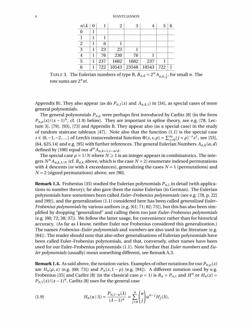
The case ρ = 1/2 also occurs in several contexts. In this case, it is often more convenientto consider the numbers Bn,k := 2n An,k,1/2 which are integers and satisfy the recursion

(1.8) Bn,k = (2k +1)Bn−1,k + (2n −2k +1)Bn−1,k−1, n> 1,

with B0,0 = 1 (and Bn,k = 0 if k ∉ {0, . . . ,n}), see [65, A060187] and Table 3. These numbersare sometimes called Eulerian numbers of type B. They seem to have been introduced byMacMahon [58, p. 331] in number theory. (It seems likely that they were used already byEuler, who in [26] also says, without giving the calculation, that he can prove similar re-sults for

∑∞k=1(−1)k (2k −1)m ; see [46] for a calculation using Pn,1/2 and methods of [26].)

The numbers Bn,k also have combinatorial interpretations, for example as the numbersof descents in signed permutations, i.e., in the hyperoctahedral group [5; 14; 76]. Fur-thermore, the numbers Bn,k and the distribution En,1/2 appear in the study of randomstaircase tableaux [17]. Pn,1/2(x) and Bn,k appear in spline theory [78, Lecture 3.4] (see

4 SVANTE JANSON

n\k 0 1 2 3 4 5 60 11 1 12 1 6 13 1 23 23 14 1 76 230 76 15 1 237 1682 1682 237 16 1 722 10543 23548 10543 722 1

TABLE 3. The Eulerian numbers of type B, Bn,k = 2n An,k, 12

, for small n. The

row sums are 2nn!.

Appendix B). They also appear (as do Pn,1(x) and An,k,1) in [34], as special cases of moregeneral polynomials.

The general polynomials Pn,ρ were perhaps first introduced by Carlitz [8] (in the formPn,ρ(x)/(x − 1)n , cf. (1.9) below). They are important in spline theory, see e.g. [78, Lec-ture 3], [79], [93], [73] and Appendix B. They appear also (as a special case) in the studyof random staircase tableaux [47]. Note also that the function (1.1) is the special cases ∈ {0,−1,−2, . . . } of Lerch’s transcendental function Φ(z, s,ρ) = ∑∞

j=0( j +ρ)−s z j , see [55],[64, §25.14] and e.g. [95] with further references. The general Eulerian Numbers An,k (a,d)defined by [100] equal our d n An,k+1,1−a/d .

The special case ρ = 1/N where N > 1 is an integer appears in combinatorics. The inte-gers N n An,k,1/N (cf. Bn,k above, which is the case N = 2) enumerate indexed permutationswith k descents (or with k exceedances), generalizing the cases N = 1 (permutations) andN = 2 (signed permutations) above, see [90].

Remark 1.3. Frobenius [35] studied the Eulerian polynomials Pn,1 in detail (with applica-tions to number theory); he also gave them the name Eulerian (in German). The Eulerianpolynomials have sometimes been called Euler–Frobenius polynomials (see e.g. [78, p. 22]and [99]), and the generalization (1.1) considered here has been called generalized Euler–Frobenius polynomials by various authors (e.g. [61; 71; 82; 73]), but this has also been sim-plified by dropping “generalized” and calling them too just Euler–Frobenius polynomials(e.g. [60; 72; 38; 37]). We follow the latter usage, for convenience rather than for historicalaccuracy. (As far as I know, neither Euler nor Frobenius considered this generalization.)The names Frobenius–Euler polynomials and numbers are also used in the literature (e.g.[84]). The reader should note that also other generalizations of Eulerian polynomials havebeen called Euler–Frobenius polynomials, and that, conversely, other names have beenused for our Euler–Frobenius polynomials (1.1). Note further that Euler numbers and Eu-ler polynomials (usually) mean something different, see Remark A.3.

Remark 1.4. As said above, the notation varies. Examples of other notations for our Pn,ρ(x)are Hn(ρ, x) (e.g. [60; 73]) and Pn(x,1 − ρ) (e.g. [94]). A different notation used by e.g.Frobenius [35] and Carlitz [8] (in the classical case ρ = 1) is Rn = Pn,1 and H n or Hn(x) =Pn,1(x)/(x −1)n . Carlitz [8] uses for the general case

(1.9) Hn(u |λ) = Pn,1−u(λ)

(λ−1)n=

n∑j=0

(n

j

)un− j H j (λ),

EULER–FROBENIUS NUMBERS AND ROUNDING 5

where the last equality follows from (A.9). Similarly, e.g. Schoenberg [78] uses An(x; t ) forour (1−t−1)−nPn,x(t−1) = (t−1)−nPn,1−x(t ) (which thus equals Hn(x | t ) in (1.9)), cf. (A.14);he further usesΠn(t ) for Pn,1(t ) and ρn(t ) for 2nPn,1/2(t ).

Remark 1.5. Many other combinatorial numbers satisfy recursion formulas similar to(1.4); see [98] for a general version. There are also many other generalizations of Euleriannumbers and polynomials that have been defined by various authors; for a few examples,see [7; 10], [9], [12], [21], [96], [84], [83], [100]. In particular, note the generalized Euleriannumbers A(r, s |α,β) defined by Carlitz and Scoville [12]; the Euler–Frobenius numbers arethe special case An,k,ρ = A(n −k,k |ρ,1−ρ).

As said above, the case ρ = 0 (or ρ = 1) of Theorem 1.2 is well-known. We end thissection by recalling the simple proof by Stanley [88] giving an explicit connection betweenbSnc and the number of descents in a random permutation, which, as said above, hasthe distribution En,1; we give it here in probabilistic formulation rather than the originalgeometric, cf. Theorem 2.1:

In the notation of Theorem 1.2, let V j be the fractional part {S j } := S j −bS j c; then V1, . . . ,Vn is another sequence of independent uniformly distributed random variables. Thus thenumber of descents in a random permutation of length n has the same distribution as∑n

i=2 1{Vi−1 >Vi }. On the other hand, Vi−1 >Vi exactly when the sequence S1, . . . ,Sn passesan integer; thus 1{Vi−1 >Vi } = bSi c−bSi−1c and this sum equals bSnc.

An extension of this proof to the case ρ = 1/N and indexed permutations is given in [90,Theorem 50]; a modification for the case ρ = 1/2 and (one version of) descents in signedpermutations is given in [76].

Section 2 gives a geometric formulation of Theorem 1.2 and some related results. Sec-tion 3 gives a proof of Theorem 1.2 together with further connections between the distri-bution of Sn and Euler–Frobenius numbers. Section 4 introduces ρ-rounding, and statesTheorem 1.2 using it. Section 5 uses this to derive results on the characteristic functionand moments of the Euler–Frobenius distribution. Section 6 shows asymptotic normalityand gives further asymptotic results. Section 7 gives applications to a well known problemon rounding. Section 8 gives applications to an election method. Finally, the appendicesgive further background and connections to other results.

We let throughout U and U1,U2, . . . denote independent uniform random variables in[0,1], and Sn :=∑n

i=1Ui .

2. VOLUMES OF SLICES

Theorem 1.2 can also be stated geometrically as follows. A proof is given in Section 3.

Theorem 2.1. Let Qn := [0,1]n be the n-dimensional unit cube and let, for s ∈ R, Qns be the

slice

(2.1) Qns :=

{(xi )n

1 ∈Qn : s −16n∑

i=1xi 6 s

}.

Then the volume of Qnk+ρ is An,k,ρ/n!, for all n> 1, k ∈Z and ρ ∈ [0,1].

As said above, the case ρ = 0 (or ρ = 1), when the volumes are given by the Euleriannumbers An,k,1, is well-known [31; 88; 45; 13; 76].

The case ρ = 1/2, which corresponds to standard rounding of Sn in Theorem 1.2, andwhere the result can be stated using the Eulerian numbers of type B Bn,k in (1.8), is treatedin [13] (with reference to an unpublished technical memorandum [87]) and in [76].

6 SVANTE JANSON

[13] gives also the (n − 1)-dimensional area of the slice {(xi )n1 ∈ Qn :

∑ni=1 xi = s}. This

equals, by simple geometry,p

n times the density function of Sn at s, which by (3.5) belowequals (except when n = 1 and s = 1)

(2.2)

pn

(n −1)!An−1,bsc,{s}.

See also [69] and [13], and the further references in the latter, for related results on moregeneral slices of cubes. Furthermore, [76] gives related results, involving Eulerian num-bers, on some slices of a simplex.

Mixed volumes of two consequtive slices Qnk and Qn

k+1 (with integer k) are studied by[22], and further by [97] where relations to our An,k,ρ (and fn+1(x) in Theorem 3.2 below)are given based on the fact [22] that the Minkowski sum λQn

k +Qnk+1 = (λ+1)Qn

k+1/(λ+1).

3. THE DISTRIBUTION OF Sn

Let Fn(x) be the distribution function and fn(x) = F ′n(x) the density function of Sn :=∑n

i=1Ui . Then f1(x), the density function of S1 =U1, is the indicator function 1[0,1] of theinterval [0,1], and fn is the n-fold convolution 1[0,1] ∗·· ·∗1[0,1]. Hence, for n> 1,

(3.1) fn+1(x) = fn ∗1[0,1](x) =∫ 1

0fn(x − y)dy = Fn(x)−Fn(x −1).

Note that the density fn(x) is continuous for n > 2, as a convolution of bounded, inte-grable functions (or by (3.1), since Fn(x) is continuous for n> 1), while f1(x) is discontin-uous at x = 0 and x = 1. We regard f1(x) as undetermined at these two points, and we willtacitly assume that x 6= 0,1 in equations involving f1(x) (such as (3.3) when n = 1).

The distribution of Sn was, as said above, calculated already by Laplace [54, pp. 257–260] (by taking the limit of a discrete version), see also e.g. Feller [28, XI.7.20] (where theresult is attributed to Lagrange) and [29, Theorem I.9.1] (with a simple proof using (3.1)and induction); the result is the following. (A more general formula for the sum of inde-pendent uniform random variables on different intervals is given by Pólya [69].) We usethe notation (x)n+ := (max(x,0))n , interpreted as 0 when x 6 0 and n> 0.

Theorem 3.1 (E.g. [54], [29]). For n> 1, Sn has the distribution function

(3.2) Fn(x) :=P(Sn 6 x) = 1

n!

n∑j=0

(−1) j

(n

j

)(x − j )n

+

and density function

(3.3) fn(x) := F ′n(x) = 1

(n −1)!

n∑j=0

(−1) j

(n

j

)(x − j )n−1

+ .

�

It is easy to see that Theorems 1.2 and 2.1 are equivalent to the following relation be-tween the densities fn and the Euler–Frobenius numbers. (The case ρ = 0 is noted in [23].Moreover, the relation is well-known in the spline setting, see e.g. [78, Theorem 3.2] (forρ = 1) and [93; 94; 81; 82]; see also (for the case ρ = 0 or 1) [97; 44].)

Theorem 3.2. For integers n> 0 and k ∈Z, and ρ ∈ [0,1],

(3.4) fn+1(k +ρ) = An,k,ρ

n!.

EULER–FROBENIUS NUMBERS AND ROUNDING 7

Equivalently, for every real x,

(3.5) fn+1(x) = An,bxc,{x}/n!.

We first verify that, as claimed above, Theorems 1.2, 2.1 and 3.2 are equivalent; we thenprove the three theorems.

Proof of Theorem 1.2 ⇐⇒ Theorem 2.1 ⇐⇒ Theorem 3.2. By replacing ρ by 1−ρ, (1.7) canbe written

(3.6) P(bSn +1−ρc = k

)= An,k,ρ

n!, ρ ∈ [0,1], k ∈Z.

In Theorem 2.1, the volume of Qns equals P

(s −16 Sn < s

). Taking s = k +ρ, we have

k +ρ−16 Sn < k +ρ ⇐⇒ k 6 Sn +1−ρ < k +1

⇐⇒ bSn +1−ρc = k,

and thus Theorem 2.1 is equivalent to (3.6).Similarly, by (3.1), at least when n> 1,

(3.7) fn+1(k +ρ) =P(k +ρ−1 < Sn 6 k +ρ) =P(bSn +1−ρc = k),

so (3.4) is equivalent to (3.6). Hence all three theorems are equivalent to (3.6). (The trivialand partly exceptional case n = 0 of Theorem 3.2 can be verified directly.) �

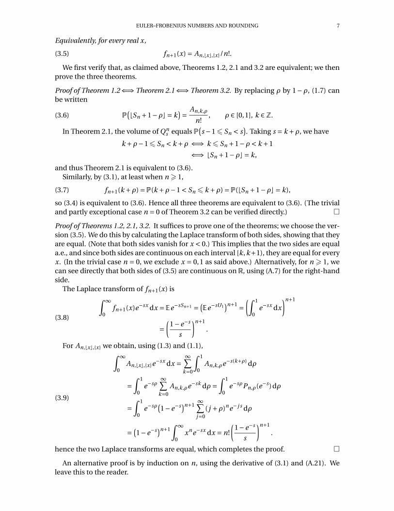
Proof of Theorems 1.2, 2.1, 3.2. It suffices to prove one of the theorems; we choose the ver-sion (3.5). We do this by calculating the Laplace transform of both sides, showing that theyare equal. (Note that both sides vanish for x < 0.) This implies that the two sides are equala.e., and since both sides are continuous on each interval [k,k+1), they are equal for everyx. (In the trivial case n = 0, we exclude x = 0,1 as said above.) Alternatively, for n > 1, wecan see directly that both sides of (3.5) are continuous on R, using (A.7) for the right-handside.

The Laplace transform of fn+1(x) is∫ ∞

0fn+1(x)e−sx dx = Ee−sSn+1 = (

Ee−sU1)n+1 =

(∫ 1

0e−sx dx

)n+1

=(

1−e−s

s

)n+1

.

(3.8)

For An,bxc,{x} we obtain, using (1.3) and (1.1),∫ ∞

0An,bxc,{x}e

−sx dx =∞∑

k=0

∫ 1

0An,k,ρe−s(k+ρ) dρ

=∫ 1

0e−sρ

∞∑k=0

An,k,ρe−sk dρ =∫ 1

0e−sρPn,ρ(e−s)dρ

=∫ 1

0e−sρ(1−e−s)n+1

∞∑j=0

( j +ρ)ne− j s dρ

= (1−e−s)n+1

∫ ∞

0xne−sx dx = n!

(1−e−s

s

)n+1

.

(3.9)

hence the two Laplace transforms are equal, which completes the proof. �

An alternative proof is by induction on n, using the derivative of (3.1) and (A.21). Weleave this to the reader.

8 SVANTE JANSON

Remark 3.3. By (3.4), the basic recursion (1.4) is equivalent to the recursion formula

(3.10) fn+1(x) = 1

n

(x fn(x)+ (n +1−x) fn(x −1)

)for the density functions fn . This formula is well-known in spline theory, see [80, (4.52)–(4.53)]. Conversely, (3.10) implies (3.4), and thus also Theorems 1.2 and 2.1, by induction.

Remark 3.4. By (3.4) and (3.3), for n> 1 and ρ ∈ [0,1],

(3.11) An,k,ρ =n+1∑j=0

(−1) j

(n +1

j

)(k +ρ− j )n

+ =k∑

j=0(−1) j

(n +1

j

)(k +ρ− j )n .

This is another well-known formula, at least for the Eulerian case ρ = 1. It has been usedto extend the definition of the Euler–Frobenius numbers to arbitrary real n by [6] (Euleriannumbers, ρ = 1) and [56] (note that A(x,n) in [56] equals our An,bxc,{x}).

We extend the definition (1.5) of En,ρ for ρ ∈ [0,1] to arbitrary real ρ by defining, for anyρ ∈R,

(3.12) En,ρ :=En,{ρ} −bρc.

As above, we use En,ρ also to denote the distribution of this random variable. Since En,0d=

En,1+1, and we only are interested in the distribution of En,ρ, (3.12) is consistent with ourprevious definition (1.5) for all ρ ∈ [0,1]. Note, however, that (1.5) holds only for ρ ∈ [0,1].(See also Remark 1.1.)

This rather trivial extension is sometimes convenient. Theorems 1.2 and 3.2 extend im-mediately:

Theorem 3.5. For any real ρ and n> 1,

(3.13) En,ρd= bSn +1−ρc

and, for any k ∈Z,

(3.14) P(En,ρ = k) =P(bSn +1−ρc = k) = An,k+bρc,{ρ}/n! = fn+1(k +ρ)

and

(3.15) P(En,ρ 6 k) =P(bSn +1−ρc6 k) = Fn(k +ρ).

Proof. By (3.12) and Theorem 1.2,

En,ρ :=En,{ρ} −bρc d= bSn +1− {ρ}c−bρc = bSn +1−ρc,

which also implies (3.15). Moreover, by (3.12), (1.5) and (3.5),

P(En,ρ = k) =P(En,{ρ} = k +bρc)= An,k+bρc,{ρ}/n! = fn+1(k +ρ). �

4. ROUNDING

Let ρ ∈ [0,1] and define ρ-rounding of real numbers by rounding a number x down (tothe nearest integer) if its fractional part {x} is less that ρ, and up (to the nearest integer)otherwise. We denote ρ-rounding by bxcρ, and can state the definition as

(4.1) bxcρ = n ⇐⇒ n −1+ρ6 x < n +ρ,

or, equivalently,

(4.2) bxcρ = bx +1−ρc.

In particular, bxc1 = bxc (rounding down), bxc0 = dxe (rounding up), except when x is aninteger, and bxc1/2 is standard rounding (except perhaps when {x} = 1/2).

EULER–FROBENIUS NUMBERS AND ROUNDING 9

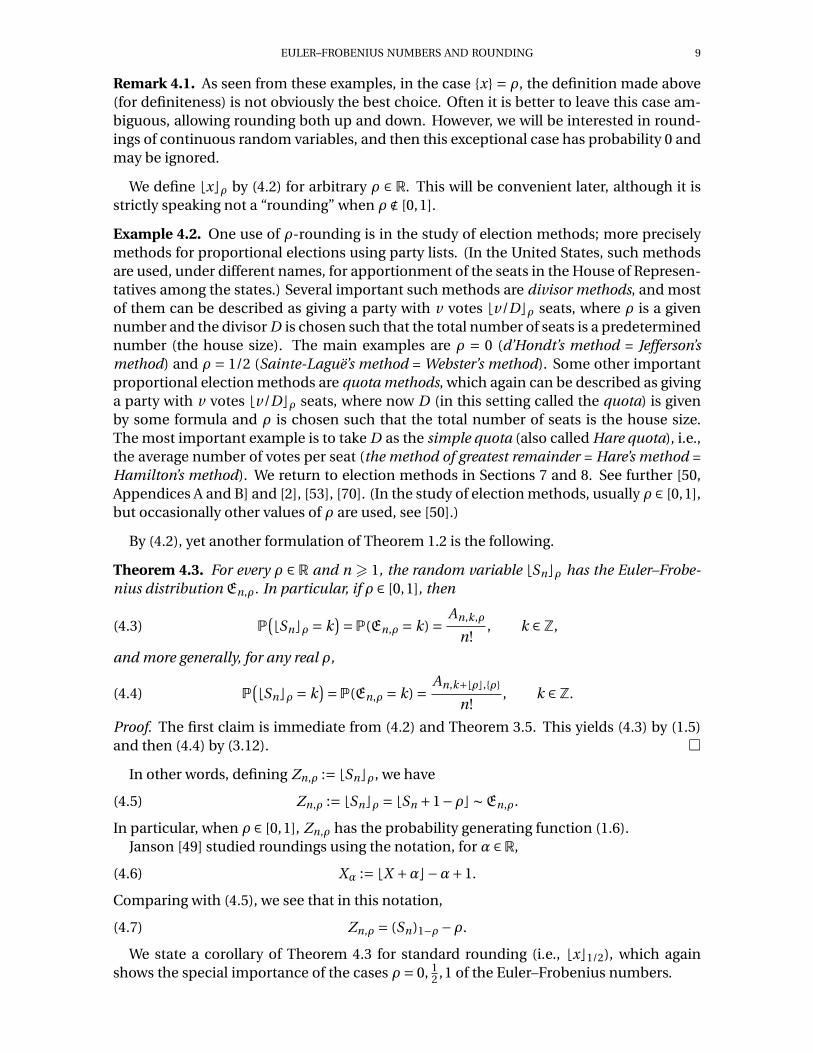
Remark 4.1. As seen from these examples, in the case {x} = ρ, the definition made above(for definiteness) is not obviously the best choice. Often it is better to leave this case am-biguous, allowing rounding both up and down. However, we will be interested in round-ings of continuous random variables, and then this exceptional case has probability 0 andmay be ignored.

We define bxcρ by (4.2) for arbitrary ρ ∈ R. This will be convenient later, although it isstrictly speaking not a “rounding” when ρ ∉ [0,1].

Example 4.2. One use of ρ-rounding is in the study of election methods; more preciselymethods for proportional elections using party lists. (In the United States, such methodsare used, under different names, for apportionment of the seats in the House of Represen-tatives among the states.) Several important such methods are divisor methods, and mostof them can be described as giving a party with v votes bv/Dcρ seats, where ρ is a givennumber and the divisor D is chosen such that the total number of seats is a predeterminednumber (the house size). The main examples are ρ = 0 (d’Hondt’s method = Jefferson’smethod) and ρ = 1/2 (Sainte-Laguë’s method = Webster’s method). Some other importantproportional election methods are quota methods, which again can be described as givinga party with v votes bv/Dcρ seats, where now D (in this setting called the quota) is givenby some formula and ρ is chosen such that the total number of seats is the house size.The most important example is to take D as the simple quota (also called Hare quota), i.e.,the average number of votes per seat (the method of greatest remainder = Hare’s method =Hamilton’s method). We return to election methods in Sections 7 and 8. See further [50,Appendices A and B] and [2], [53], [70]. (In the study of election methods, usually ρ ∈ [0,1],but occasionally other values of ρ are used, see [50].)

By (4.2), yet another formulation of Theorem 1.2 is the following.

Theorem 4.3. For every ρ ∈ R and n > 1, the random variable bSncρ has the Euler–Frobe-nius distribution En,ρ. In particular, if ρ ∈ [0,1], then

(4.3) P(bSncρ = k

)=P(En,ρ = k) = An,k,ρ

n!, k ∈Z,

and more generally, for any real ρ,

(4.4) P(bSncρ = k

)=P(En,ρ = k) = An,k+bρc,{ρ}

n!, k ∈Z.

Proof. The first claim is immediate from (4.2) and Theorem 3.5. This yields (4.3) by (1.5)and then (4.4) by (3.12). �

In other words, defining Zn,ρ := bSncρ, we have

(4.5) Zn,ρ := bSncρ = bSn +1−ρc ∼En,ρ.

In particular, when ρ ∈ [0,1], Zn,ρ has the probability generating function (1.6).Janson [49] studied roundings using the notation, for α ∈R,

(4.6) Xα := bX +αc−α+1.

Comparing with (4.5), we see that in this notation,

(4.7) Zn,ρ = (Sn)1−ρ−ρ.

We state a corollary of Theorem 4.3 for standard rounding (i.e., bxc1/2), which againshows the special importance of the cases ρ = 0, 1

2 ,1 of the Euler–Frobenius numbers.

10 SVANTE JANSON

Corollary 4.4. Let U1, . . . ,Un be independent random variables uniformly distributed on[−1

2 , 12 ], and let Sn :=∑n

i=1Ui , with n> 1. Then, bSnc1/2 has the distribution En,(n+1)/2, andthus, for k ∈Z,

P(bSnc1/2 = k

)={An,k+n/2,1/2/n!, n even,

An,k+(n+1)/2,0/n! = An,k+(n−1)/2,1/n!, n odd.

Proof. We can take Ui :=Ui − 12 , and then, using (4.5),

bSnc1/2 =⌊

Sn + 1

2

⌋=

⌊Sn − n −1

2

⌋= ⌊

Sn⌋

(n+1)/2d=En,(n+1)/2.

The result follows by (4.4). �

5. CHARACTERISTIC FUNCTION AND MOMENTS

We use the results in Section 4 to derive further results for the Euler–Frobenius distribu-tion En,ρ. As said in the introduction, we also use En,ρ to denote a random variable with

this distribution. Since En,ρd= Zn,ρ by (4.5), we can just as well consider Zn,ρ := bSncρ.

We begin with an expression for the characteristic function and moment generatingfunction of the Euler–Frobenius distribution En,ρ. (Cf. [37, Lemma 2.4] where an equiv-alent formula is given.) We denote the characteristic function of a random variable X byϕX . Note that if ρ ∈ [0,1] (and the general case can be reduced to this by (3.12)), we haveby (1.6)

(5.1) ϕEn,ρ (t ) := Ee itEn,ρ = Pn,ρ(e it )

n!and, more generally, for all t ∈C, the moment generating function

(5.2) Ee tEn,ρ = Pn,ρ(e t )

n!.

Theorem 5.1. Let n> 1 and ρ ∈R. The characteristic function of En,ρ is given by

(5.3) ϕEn,ρ (t ) = i−n−1e−iρt (e it −1)n+1

∞∑k=−∞

e−2πikρ

(t +2πk)n+1.

Equivalently, the moment generating function is, for all t ∈C,

(5.4) Ee tEn,ρ = e−ρt (e t −1)n+1

∞∑k=−∞

e−2πikρ

(t +2πki)n+1.

(For t ∈ 2πZ or t ∈ 2πiZ, respectively, the expressions are interpreted by continuity.)

Proof. This can be reduced to the case ρ ∈ [0,1], and then (5.3) is (5.1) together with a spe-cial case of an expansion found by Lerch [55, (4) and (5)] (take s =−n there); nevertheless,we give a probabilistic proof (valid for all ρ) using a general formula for rounded stochasticvariables in [49].

Since Ui has the characteristic function

(5.5) ϕU (t ) := Ee itU = e it −1

it,

the sum Sn has the characteristic function

(5.6) ϕSn (t ) =ϕU (t )n =(e it −1

it

)n.

EULER–FROBENIUS NUMBERS AND ROUNDING 11

The formula in [49, Theorem 2.1] now yields

Ee it (Sn )1−ρ =∞∑

k=−∞e2πik(1−ρ)ϕU (t +2πk)ϕSn (t +2πk)

=∞∑

k=−∞e2πik(1−ρ)

(e it −1

i(t +2πk)

)n+1

,

which yields (5.3) by (4.5) and (4.7).This derivation tacitly assumes that t is real, but the sum in (5.3) converges for every

complex t ∈ C \ 2πZ, and defines a meromorphic function with poles in 2πZ; thus theright-hand side of (5.3) is an entire function of t ∈ C. So is also the left-hand side, since itis a trigonometric polynomial. Hence (5.3) is valid for all complex t , and replacing t by t/i,we obtain (5.4). �

Moments of arbitrary order can be obtained from the moment generating function bydifferentiation. For moments of order at most n, this leads to simple results.

Lemma 5.2. Let n > 1 and ρ ∈ R. The random variables En,ρ +ρ and Sn+1 have the samemoments up to order n:

(5.7) E(En,ρ+ρ

)m = ESmn+1, 16m6 n.

Proof. Since En,ρ+ρ d= Zn,ρ+ρ = (Sn)1−ρ by (4.7), this follows by [49, Theorem 2.3], notingthat

(5.8) ϕ(t ) := e it −1

itϕSn (t ) =

(e it −1

it

)n+1

has its n first derivatives 0 at t = 2πn, n ∈Z\{0}. (Alternatively and equivalently, this followsfrom (5.4), noting that the terms with k 6= 0 give no contribution to the m:th derivative att = 0 for m6 n, since the factor (e t −1)n+1 vanishes to order n +1 there.) �

This leads to the following results, shown by Gawronski and Neuschel [37, Lemmas 4.1and 4.2] by related but more complicated calculations. (In the classical case ρ = 1, thecumulants were given already by David and Barton [18, p. 153].)

Theorem 5.3. For any ρ ∈R,

(5.9) EEn,ρ = n +1

2−ρ, n> 1,

and

(5.10) VarEn,ρ = n +1

12, n> 2.

More generally, for 2 6 m 6 n, the m:th cumulant κm(En,ρ) is independent of ρ, and isgiven by

(5.11) κm(En,ρ) =κm(Sn+1) = (n +1)κm(U ) = (n +1)Bm

m, 26m6 n,

where Bm is the m:th Bernoulli number. In particular, κm(En,ρ) = 0 if m is odd with 3 6m6 n.

For Bernoulli numbers, see e.g. [39, Section 6.5] and [64, §24.2(i)].

12 SVANTE JANSON

Proof. For the mean we have by Lemma 5.2, for n> 1,

(5.12) EEn,ρ+ρ = ESn+1 = (n +1)EU = n +1

2,

which gives (5.9).For higher moments, we note that the m:th cumulant κm can be expressed as a poly-

nomial in moments of order at most m; hence Lemma 5.2 implies that κm(En,ρ +ρ) =κm(Sn+1) for m 6 n. Moreover, for any random variable (with E |X |m < ∞) and any realnumber a, κm(X +a) =κm(X ), since κm(X +a) is the m:th derivative at 0 of logEe t (X+a) =at + logEe t X . Hence,

(5.13) κm(En,ρ) =κm(En,ρ+ρ) =κm(Sn+1), 26m6 n.

Furthermore, since Sn+1 is the sum of the n + 1 i.i.d. random variables Ui , i 6 n + 1,κm(Sn+1) = (n + 1)κm(U ). Finally, the cumulants of the uniform distribution are givenby κm(U ) = Bm/m for m> 2; this, as is well-known, is shown by a simple calculation: (for|t | < 2π; see [64, §24.2.1] for the last step)

∞∑m=0

mκm(U )t m

m!= t

d

dt

∞∑m=0

κm(U )t m

m!= t

d

dtlogEe tU = t

d

dtlog

e t −1

t

= te t

e t −1−1 = t

e t −1+ t −1 =

∞∑m=0

Bmt m

m!+ t −1.

Combining these facts gives (5.11). The special case m = 2 yields (5.10), since κ2 is thevariance and B2 = 1/6. �

We note also that Theorem 3.2 and Fourier inversion for the distribution of Sn+1 yieldthe following integral formula. (This is well-known in the settings of Sn , and also forsplines, see e.g. [77, Theorem 3].) The case ρ = 0 is given by [63], see also [97]. (Thisintegral formula is used in [63] to define an extension A(n, x) of Eulerian numbers to realx, which by (5.14) equals the Euler–Frobenius number An,bxc,{x}. The formula is furtherextended to real n in [56]; see also Remark 3.4.) The special cases (5.15)–(5.16) are givenby [37].

Theorem 5.4. If n> 1, k ∈Z and ρ ∈ [0,1], then

An,k,ρ =n!

π

∫ ∞

−∞e it (2k+2ρ−n−1)

(sin t

t

)n+1dt

= n!2

π

∫ ∞

0cos

(t (2k +2ρ−n −1)

)(sin t

t

)n+1dt .

(5.14)

In particular, for k > 1,

A2k−1,k,0 = (2k −1)!2

π

∫ ∞

0

(sin t

t

)2kdt ,(5.15)

A2k,k,1/2 = (2k)!2

π

∫ ∞

0

(sin t

t

)2k+1dt .(5.16)

Proof. By Theorem 3.2, Fourier inversion using (5.6), and finally replacing t by 2t ,

An,k,ρ

n!= fn+1(k +ρ) = 1

2π

∫ ∞

−∞e−it (k+ρ)ϕSn+1 (t ) dt

= 1

2π

∫ ∞

−∞e−it (k+ρ)

(e it −1

it

)n+1dt

= 1

π

∫ ∞

−∞e it (n+1−2k−2ρ)

(sin t

t

)n+1dt

EULER–FROBENIUS NUMBERS AND ROUNDING 13

and the result follows by replacing t by −t , noting that sin t/t is an even function. �

6. ASYMPTOTIC NORMALITY AND LARGE DEVIATIONS

It is well-known that the Eulerian distribution En,0 or En,1 is asymptotically normal, andthat furthermore a local limit theorem holds, i.e., the Eulerian numbers An,k,1 = An,k+1,0

can be approximated by a Gaussian function for large n. This has been proved by variousauthors using several different methods, see below; most of the methods generalize toEn,ρ

and An,k,ρ for arbitrary ρ ∈ [0,1]. The basic central limit theorem for En,ρ can be stated asfollows. (Recall that the mean and variance are given by Theorem 5.3.)

Theorem 6.1. En,ρ is asymptotically normal as n →∞, for any real ρ, i.e.,

(6.1)En,ρ−EEn,ρ

(VarEn,ρ)1/2d−→ N (0,1)

or, more explicitly and simplified,

(6.2)En,ρ−n/2

n1/2d−→ N

(0,

1

12

).

Proof. Immediate by (4.5) and the central limit theorem for Sn = ∑ni=1Ui . Alternatively,

the theorem follows by the method of moments from the formula (5.11) for the cumulantsin Theorem 5.3, which implies that the normalized cumulants κm(En,ρ/(VarEn,ρ)1/2) con-verge to 0 for any m> 3. Several other proofs are described below. �

One refined verison is the following local limit theorem with an asymptotic expansionproved by Gawronski and Neuschel [37]; we let as in (5.11) Bm denote the Bernoulli num-bers and let Hm(x) denote the Hermite polynomials, defined e.g. by

(6.3) Hm(x) := (−1)mex2/2 dm

dxme−x2/2,

see [66, p. 137]. (These are the orthogonal polynomials for the standard normal distribu-tion, see e.g. [48].)

Theorem 6.2 (Gawronski and Neuschel [37]). There exist polynomials qν, ν> 1, such that,for any `> 0, as n →∞, uniformly for all k ∈Z and ρ ∈ [0,1],

(6.4)An,k,ρ

n!=

√6

π(n +1)e−x2/2

(1+ ∑

ν=1

qν(x)

(n +1)ν

)+O

(n−`−3/2

),

where

(6.5) x =(k +ρ− n +1

2

)√ 12

n +1.

Explicitly,

(6.6) qν(x) = 12ν∑

H2ν+2s(x)6sν∏

m=1

1

km !

(B2m+2

(m +1)(2m +2)!

)km

,

summing over all non-negative integers (k1, . . . ,kν) with k1 +2k2 +·· ·+νkν = ν and lettings = k1 +·· ·+kν.

The polynomial qν(x) has degree 4ν. The first two are:

q1(x) =− 1

20H4(x) =−x4 −6x2 +3

20,(6.7)

14 SVANTE JANSON

q2(x) = 1

800H8(x)+ 1

105H6(x) = 21x8 −428x6 +2010x4 −1620x2 −195

16800.(6.8)

Remark 6.3. We state Theorem 6.2 using an expansion in negative powers of n + 1. Ofcourse, it is possible to use powers of n instead, but then the polynomials qi (x) will bemodified.

Before giving a proof of Theorem 6.2, we give some history and discuss various methods.The perhaps first proof of asymptotic normality for Eulerian numbers (i.e., Theorem 6.1 inthe classical case ρ = 1) was given by David and Barton [18], using the generating function(A.11) below to calculate cumulants. Bender [3, Example 3.5] used (for the equivalent caseρ = 0) instead a singularity analysis of the generating function (A.11) to obtain this andfurther results; see also Flajolet and Sedgewick [30, Example IX.12, p. 658].

The representation (A.23) of En,ρ as a sum of independent (but not identically dis-tributed) Bernoulli variables was used by Carlitz et al [11] to show asymptotic normality(global and local central limit theorems and a Berry–Esseen estimate) for Eulerian num-bers (i.e. for ρ = 0). Siraždinov [86] gave (also for ρ = 0) a local limit theorem includingthe second order term (ν= 1) in Theorem 6.2. (We have not been able to obtain the orig-inal reference, but we believe he used this representation.) More recently, Gawronski andNeuschel [37] have used this method for a general ρ ∈ [0,1] to show a global central limittheorem and the refined local limit theorem Theorem 6.2 above.

Furthermore, (A.23) was also used (for ρ = 0) by Bender [3] to obtain a local limit the-orem from the global central limit theorem (proved by him by other methods, as saidabove).

Tanny [92] showed global and local central limit theorems (for ρ = 0) using the repre-

sentation En,0d= bSnc+1, see our Theorems 1.2 and 3.5, together with the standard central

limit theorem for Sn ; see also Sachkov [75, Section 1.3.2]. This too extends to arbitrary ρ.Esseen [23] used instead (still for ρ = 0) the relation given here as (3.4) with the density

function of Sn+1, together with the standard local limit theorem for Sn . This too extends toarbitrary ρ, and is perhaps the simplest method to obtain local limit theorems. Moreover,as noted by [23], it easily yields an asymptotic expansion with arbitrary many terms as inTheorem 6.2. (For ρ = 0, [23] gave the second term explicitly; as mentioned above, thisterm was also given by Siraždinov [86].) Furthermore, the first three terms (ν6 2) in The-orem 6.2 were given (for arbitrary ρ) by Nicolas [63], using essentially the same method,but stated in analytic formulation rather than probabilistic. (See also, for the case ρ = 0,[101].)

Esseen [23] also pointed out that En,1 =En,0 −1, regarded as the number of descents ina random permutation, can be represented as

(6.9) En,1d=

n−1∑i=1

1{Ui >Ui+1},

where U1,U2, . . . are i.i.d. with the distribution U (0,1); the global central limit theorem thusfollows immediately from the standard central limit theorem for m-dependent sequences.(However, we do not know any similar representation for the case ρ ∈ (0,1).)

Proof of Theorem 6.2. We use the method of [23], and note that the theorem follows im-mediately from (3.4) and the local limit theorem for fn(x), see e.g. [66, Theorem VII.15 and(VI.1.14)], using κm(Ui ) = Bm/m for m> 2 and noting that Bm = 0 for odd m> 3. (As saidabove, the proof in [37] is somewhat different, although it also uses [66].) �

EULER–FROBENIUS NUMBERS AND ROUNDING 15

Remark 6.4. By using [66, Theorem VII.17] in the proof of Theorem 6.2 (and taking asmany terms as needed), the error term in (6.4) is improved to O

((1+|x|K )−1n−`−3/2

), for

any fixed K > 0. This is, however, a superficial improvement, since this is trivial for k +ρ ∉[0,n +1] (when An,k,ρ = 0), and otherwise easily follows from (6.4) by increasing `.

Although Theorem 6.2 holds uniformly for all k, it is of interest mainly when k = n/2+O(

√n logn), when x =O(

√logn), since for |k−n/2| larger, the main term in (6.4) is smaller

than the error term. (This holds also for the improved version in Remark 6.4.) However,we can also easily obtain asymptotic estimates for other k by the same method, now using(3.4) and large deviation estimates for the density fn+1(x), which are obtained by stan-dard arguments. (The saddle point method, which in this context is essentially the sameas using Cramér’s [16] method of conjugate distributions. See e.g. [19, Chapter 2] or [51,Chapter 27] for more general large deviation theory, and [30] for the saddle point method.)In the classical case ρ = 0, this was done by Esseen [23] (for 16 k 6 n), improving an ear-lier result by Bender [3] (εn6 k 6 (1−ε)n for any ε> 0) who used a related argument usingthe generating function (A.11). The result extends immediately to any ρ as follows.

Let ψ(t ) be the moment generating function of U ∼U (0,1), i.e.,

(6.10) ψ(t ) := Ee tU = e t −1

t

(which is an entire function), and let for a ∈ (0,1)

(6.11) m(a) := min−∞<t<∞e−atψ(t ).

Since logψ(t ) is convex (a general property of moment generating functions, and easilyverified directly in this case), and the derivative (logψ)′ increases from 0 to 1, the mini-mum is attained at a unique t (a) ∈ (−∞,∞) for each a ∈ (0,1), which is the solution to theequation

(6.12) a = (logψ)′(t ) = e t

e t −1− 1

t= 1

1−e−t− 1

t.

Set

(6.13) σ2(a) := (logψ)′′(t (a)) = 1

t (a)2− e t (a)

(e t (a) −1)2= 1

t (a)2− 1

4sinh2(t (a)/2),

interpreted (by continuity) as (logψ)′′(0) = 1/12 when a = 1/2 and thus t (a) = 0.

Theorem 6.5. Assume ρ ∈ [0,1] and 0 < k +ρ < n +1. Then

(6.14)An,k,ρ

n!= m(a)n+1√

2π(n +1)σ2(a)

(1+O(n−1)

),

where a := (k +ρ)/(n +1), uniformly in all k and ρ such that 0 < k +ρ < n +1.

Proof. We follow Esseen [23], with some details added. (As said above, this is an applica-tion of the saddle point method, using standard types of estimates. We nevertheless give adetailed proof for completeness.)

We let t = t (a), satsfying (6.12), and σ2 =σ2(a), given by (6.13).By (3.4), and replacing n by n −1, the statement is equivalent to the estimate

(6.15) fn(x) = m(a)n√2πσ2(a)n

(1+O(n−1)

),

16 SVANTE JANSON

where x = k + ρ = na, uniformly for x ∈ (0,n). To see (6.15), we use Fourier inversion(assuming n> 2), noting that the characteristic function of Sn is Ee isSn =ψ(is)n , and shiftthe line of integration to the saddle point t = t (a):

fn(x) = 1

2π

∫ ∞

−∞e−ixsψ(is)n ds = 1

2πi

∫ ∞i

−∞i

(e−azψ(z)

)n dz

= 1

2πi

∫ t+∞i

t−∞i

(e−azψ(z)

)n dz = 1

2π

∫ ∞

−∞ψ

(t + i u

)n du,

(6.16)

where ψ(z) := e−azψ(z). Note that

(6.17) ψ(t ) = e−atψ(t ) = m(a),

by (6.11) and the definition of t = t (a). Define

(6.18) Gt (u) := ψ(t + iu)

ψ(t )= e−iauψ(t + iu)

ψ(t ).

Then (6.16)–(6.17) yield

fn(x)

m(a)n= 1

2π

∫ ∞

−∞ψ

(t + i u

)n

ψ(t )ndu = 1

2π

∫ ∞

−∞Gt (u)n du.(6.19)

Note that Gt (0) = 1, while for any u 6= 0, |ψ(t + iu)| = |Ee(t+iu)U | < Ee tU =ψ(t ) and thus

(6.20) |Gt (u)| < 1, u 6= 0.

Let

(6.21) g t (u) := logGt (u) = logψ(t + iu)− logψ(t )− iau.

Then, using (6.12)–(6.13),

g t (0) = 0,(6.22)

g ′t (0) = 0,(6.23)

g ′′t (0) =−σ2,(6.24)

and, if |u|6π or |t |> 1, say,

g ′′′t (u) =O

((1+|t |)−3),(6.25)

g ′′′′t (u) =O

((1+|t |)−4).(6.26)

Consider first |t |6 10, say. Then, by a Taylor expansion and (6.22)–(6.26),

(6.27) g t (u) =−σ2

2u2 +b1(t )u3 +O(u4), |u|6π,

with b1(t ) = O(1). Hence, there exists c1 > 0 such that if |u|6 c1, then g t (u)6−σ2

3 u2, andit follows that if |s|6 c1

pn, then (consider the cases |s|6 n1/6 and |s| > n1/6 separately)

Gt

( spn

)n = exp(ng t

( spn

))= exp

(−σ

2

2s2 +b1(t )

s3

pn+O

( s4

n

))=

(1+b1(t )

s3

pn+O

( s4 + s6

n

))e−σ2s2/2 +O

(n−99e−σ2s2/4

).

Thus, since∫ c1

pn

−c1p

ns3e−σ2s2/2 ds = 0,

pn

∫ c1

−c1

Gt (u)n du =∫ c1

pn

−c1p

nGt

( spn

)nds =

∫ ∞

−∞e−σ2s2/2 ds +O

(n−1)

EULER–FROBENIUS NUMBERS AND ROUNDING 17

=p

2π

σ+O

(n−1).(6.28)

Furthermore, by (6.10), there exists C1,C2 such that for |t |6 10 and all u,

(6.29) |Gt (u)| = |ψ(t + iu)|ψ(t )

6C1|ψ(t + iu)|6 C2

|t + iu| 6C2

|u| .

Hence, ∫|u|>2C2

|Gt (u)|n du6 2∫ ∞

2C2

C n2 u−n du =O(2−n).(6.30)

Finally, by (6.20), continuity and compactness, there exists c2 > 0 such that if |t | 6 10and c16 |u|6 2C2, then

(6.31) |Gt (u)|6 1− c2,

and thus ∫c16|u|62C2

|Gt (u)|n du6 4C2(1− c2)n =O(e−c2n).(6.32)

The result (6.15) in the case |t |6 10 follows from (6.19), (6.28), (6.30), (6.32) and the obvi-ous σ2 =O(1).

For |t | > 10 we argue similarly, noting that now it follows from (6.13) that t−2 > σ2 >0.9 t−2, and thus

(6.33) 0.96 |t |σ6 1, |t |> 10.

Instead of (6.27) we now obtain, see (6.25)–(6.26),

(6.34) g t (u) =−σ2

2u2 +b1(t )u3 +O(|t |−4u4), −∞< u <∞,

with bi (t ) =O(|t |−3). Hence, there exists c3 > 0 such that if |u|6 c3|t |, then g t (u)6−σ2

3 u2,and thus, if |s|6 c3

pn, then

Gt

( t spn

)n = exp(−σ

2t 2

2s2 + t 3b1(t )

s3

pn+O

( s4

n

))=

(1+ t 3b1(t )

s3

pn+O

( s4 + s6

n

))e−σ2t 2s2/2 +O

(n−99e−σ2t 2s2/4

).

Thus, recalling (6.33),p

n

|t |∫ c3|t |

−c3|t |Gt (u)n du =

∫ c3p

n

−c3p

nGt

( |t |spn

)nds =

∫ ∞

−∞e−σ2t 2s2/2 ds +O

(n−1)

=p

2π

|t |σ +O(n−1).(6.35)

Furthermore, by (6.18) and (6.10), for |t |> 10,

(6.36) |Gt (u)| = |e t+iu −1||e t −1|

|t ||t + iu| 6

e t +1

|e t −1||t |

|t + iu| 6 1.1|t ||u| .

Hence, ∫|u|>3|t |

|Gt (u)|n du6 2∫ ∞

3|t |(1.1 |t |)nu−n du =O(|t |2−n).(6.37)

18 SVANTE JANSON

Finally, by (6.36), for |t |> 10 and |u|> c3|t |,

(6.38) |Gt (u)| = e t +1

|e t −1||t |

|t + iu| 6e t +1

|e t −1|1√

1+ c23

.

Let 0 < c4 < 1− (1+ c23)−1/2. Since (e t +1)/|e t −1| → 1 as t →±∞, there exists C3 such that

if |t |>C3 and |u|> c3|t |, then

(6.39) |Gt (u)|6 1− c4,

For 10 6 |t | 6 C3 and c3|t | 6 |u| 6 3|t |, the same holds by (6.20) and compactness, pro-vided we decrease c4 to be small enough. Hence,∫

c3|t |6|u|63|t ||Gt (u)|n du6 6|t |(1− c4)n =O(|t |e−c4n).(6.40)

The result (6.15) in the case |t |> 10 follows from (6.19), (6.35), (6.37), (6.40) and (6.33). �

As remarked by Esseen [23], it is possible to obtain an expansion with further terms in(6.14) by the same method.

The saddle point method is standard in problems of this type. However, it is perhapssurprising that it can be used with a uniform relative error bound for all t (a) ∈ (−∞,∞).

7. MORE ON ROUNDING

Let p1, . . . , pn be given probabilities (or proportions) with∑n

i=1 pi = 1 and let N be a(large) integer. Suppose that we want to round N pi to integers, by standard rounding or,more generally, by ρ-rounding for some given ρ ∈ R. It is often desirable that the sum ofthe results is exactly N , but this is, of course, not always the case. We thus consider thediscrepancy

(7.1) ∆ρ :=n∑

i=1bN pi cρ−N .

More generally, we may round (N+γ)pi for some fixed γ ∈R and we define the discrepancy

(7.2) ∆ρ,γ :=n∑

i=1b(N +γ)pi cρ−N .

Example 7.1. If a statistical table is presented as percentages, with all percentages roundedto integers, we have this situation with N = 100; the percentages do not necessarily add upto 100, and the error is given by ∆1/2. Rounding to other accuracies correspond to othervalues of N . This has been studied by several authors, see Mosteller, Youtz and Zahn [62]and Diaconis and Freedman [20].

Example 7.2. The general idea of a proportional election method is that a given num-ber N of seats are to be distributed among n parties which have obtained v1, . . . , vn votes.With pi := vi /

∑nj=1 v j , the proportion of votes for party i , the party should ideally get N pi

seats, but the number of seats has to be an integer so some kind of rounding procedure isneeded. (See Example 4.2 and the reference given there for some important methods usedin practice.)

A simple attempt would be to round N pi to the nearest integer and give bN pi c1/2 seatsto party i . More generally, we might fix some ρ ∈ [0,1] and give the party bN pi cρ seats. Ofcourse, this is not a workable election method since the sum in general is not exactly equalto N , and the error is given by ∆ρ. (In principle the method could be used for elections ifone accepts a varying size of the elected house, but I don’t know any examples of it being

EULER–FROBENIUS NUMBERS AND ROUNDING 19

used.) Nevertheless, this can be seen as the first step in an algorithm implementing divisormethods, see Happacher and Pukelsheim [41] and Pukelsheim [70]. In this context it isalso useful to consider the more general b(N +γ)pi cρ for some given γ ∈ R, see again [41]and [70]; then the error is given by (7.2).

Example 7.3. Roundings of (N +γ)pi and thus (7.2) occur also in the study of quota meth-ods of elections, for example Droop’s method where we take γ = 1 and adjust ρ to obtainthe sum N , see [50, Appendix B].

If we assume that the proportions pi are random, it is thus of interest to find the distri-bution of the discrepancy ∆ρ,γ, and in particular of ∆ρ,0 =∆ρ. We consider the asymptoticdistribution of ∆ρ,γ as N →∞.

The simplest assumption is that (p1, . . . , pn) is uniformly distributed over the n − 1-dimensional unit simplex {(pi )n

1 ∈ Rn+ :∑

i pi = 1}, but it turns out (by Weyl’s lemma, seee.g. [50, Lemma 4.1 and Lemma C.1]) that the asymptotic distribution is the same for anyabsolutely continuous distribution of (pi )n−1

1 , and we state our results for this setting.

Remark 7.4. Alternatively, it is also possible to consider a fixed vector (pi )n1 (for almost all

choices) and let N be random as in [50, Section 1] (with Np−→∞). The same asymptotic

results are obtained in this case too, but we leave the details to the reader.

In the standard case ρ = 1/2 and γ = 0, the asymptotic distribution of the discrepancy∆1/2 was found by Diaconis and Freedman [20], assuming (as we do here) that (pi )n

1 havean absolutely continuous distribution on the unit simplex. (The cases n = 3,4, with uni-formly distributed probabilities (pi )n

1 , were earlier treated by Mosteller, Youtz and Zahn[62].) This was extended to ∆ρ with arbitrary ρ (still with γ = 0) by Balinski and Rachev[1]. Happacher and Pukelsheim [41; 42] considered general ρ and γ (assuming uniformlydistributed (pi )n

1 ) and found asymptotics of the mean and variance of ∆ρ,γ [41] and (atleast in the case γ = n(ρ− 1

2 )) the asymptotic distribution [42]. The exact distribution of∆ρ,γ for a finite N (assuming uniform (pi )n

1 ) was given by Happacher [40, Sections 2 and3]. Furthermore, asymptotic results for the probability P(∆ρ,γ = 0) of no discrepancy havealso been given (assuming uniform (pi )n

1 ) by Kopfermann [53, p. 185] (ρ = 1/2, γ= 0), andGawronski and Neuschel [37] (ρ = 1/2, γ = 0); the latter paper moreover gives the con-nection to Euler–Frobenius numbers. (The other papers referred to here state the resultsusing Sn−1 or the density function fn of Sn , or the explicit sum in (3.3) for the latter.)

We state and extend these asymptotic results for ∆ρ,γ as follows. Equivalent reformu-lations of (7.3)–(7.4) (including the versions in the references above) can be given using(3.14), see also (7.9) below.

Theorem 7.5. Suppose that (p1, . . . , pn) are random with an absolutely continuous distri-bution on the n −1-dimensional unit simplex. Then, as N →∞, for any fixed real ρ and γ,n> 2 and k ∈Z,

(7.3) ∆ρ,γd−→En−1,nρ−γ.

In other words,

(7.4) P(∆ρ,γ = k) → An−1,k+bnρ−γc,{nρ+γ}

(n −1)!.

Furthermore,

E∆ρ,γ→ EEn−1,nρ−γ = n(1

2−ρ

)+γ(7.5)

20 SVANTE JANSON

and if n> 3,

Var∆ρ,γ→ VarEn−1,nρ−γ = n

12.(7.6)

Proof. Let Xi := (N +γ)pi +1−ρ and Yi := {Xi }. Thus, by the definition (4.2), b(N +γ)pi cρ =bXi c and hence by (7.2),

∆ρ,γ =n∑

i=1bXi c−N =

n∑i=1

(Xi −Yi )−N

= N +γ+n(1−ρ)−n∑

i=1Yi −N

= γ+n(1−ρ)−n∑

i=1Yi .

(7.7)

Since this is an integer, and Yn ∈ [0,1), it follows that

(7.8) ∆ρ,γ =⌊γ+n(1−ρ)−

n−1∑i=1

Yi

⌋.

As N →∞, the fractional parts ({N pi })n−11 converge jointly in distribution to the indepen-

dent uniform random variables (Ui )n−11 , see [50, Lemma C.1], and since Yi = {{N pi }+γpi +

1−ρ}, the same holds for (Yi )n−11 . Thus (7.8) implies, using 1−Ui

d=Ui ,

∆ρ,γd−→

⌊γ+n(1−ρ)−

n−1∑i=1

Ui

⌋d=

⌊γ+1−nρ+

n−1∑i=1

Ui

⌋= ⌊

γ+1−nρ+Sn−1⌋= bSn−1cnρ−γ.

(7.9)

Since bSn−1cnρ−γd=En−1,nρ−γ by Theorem 4.3, this proves (7.3); furthermore, Theorem 4.3

yields also (7.4). Since ∆ρ,γ is uniformly bounded by (7.7), (7.3) implies moment conver-gence and thus (7.5)–(7.6) follow by Theorem 5.3. �

Remark 7.6. In the case of uniformly distributed probabilities (pi )n1 , Happacher and Pu-

kelsheim [41] have given a more precise form of the moment asymptotics (7.5)–(7.6) withexplicit higher order terms.

Example 7.7. We see from (7.5) that the choice γ = n(ρ− 12 ) yields E∆ρ,γ → 0, so the dis-

crepancy is asymptotically unbiased. This was shown by Happacher and Pukelsheim [41],who therefore recommend this choice of γ when the aim is to try to avoid a discrepancy;see also [42].

For standard rounding, ρ = 1/2 and γ= 0, Theorem 7.5 yields the result of Diaconis andFreedman [20], which we state as a corollary.

Corollary 7.8. With assumptions as in Theorem 7.5,

(7.10) ∆1/2d−→En−1,n/2.

In other words,

(7.11) P(∆1/2 = k) → An−1,k+bn/2c,{n/2}

(n −1)!.

Using the notation of Corollary 4.4, the result can also be written

(7.12) ∆1/2d−→bSn−1c1/2.

EULER–FROBENIUS NUMBERS AND ROUNDING 21

Proof. Theorem 7.5 yields (7.10)–(7.11), and (7.12) then follows by Corollary 4.4. �

The asymptotic distribution in Corollary 7.8 can also be described as En−1,0 when n iseven and En−1,1/2 when n is odd, in both cases centred by subtracting the mean bn/2c.Note that in this case the asymptotic distribution is symmetric, e.g. by (A.16).

Example 7.9. Taking k = 0 in Corollary 7.8 we obtain the asymptotic probability that stan-dard rounding yields the correct sum:

(7.13) P(∆1/2 = 0) → An−1,bn/2c,{n/2}/(n −1)!.

The limit is precisely the value for P(bSn−1c1/2 = 0

)given by Corollary 4.4.

Remark 7.10. Even if (p1, . . . , pn) is uniformly distributed, the result in Theorem 7.5 is ingeneral only asymptotic and not exact for finite N because of edge effects. For a simpleexample, if ρ = 1/2 and N = 1, thenP(∆1/2 = 0) =P(∑n

1 bpi c1/2 = 1)= nP

(p1 > 1/2

)= n21−n ,which differs from the asymptotical value in (7.13) for n > 4. (It is much smaller for largen, since it decreases exponentially in n.) See [40] for an exact formula for finite N .

8. EXAMPLE: THE METHOD OF GREATEST REMAINDER

By (3.15), (3.12) and (1.5), the distribution function Fn of Sn can be expressed usingthe Euler–Frobenius distribution or using Euler–Frobenius numbers. As another exampleinvolving election methods, consider again an election as in Example 7.2, with N seatsdistributed among n> 3 parties having proportions p1, . . . , pn of the votes. Let s1, . . . , sn bethe number of seats assigned to the parties by the method of greatest remainder (Hare’smethod; Hamilton’s method), see Example 4.2, and consider the bias ∆′

1 := s1 − N p1 forparty 1. Let again the vector (p1, . . . , pn) be random as in Theorem 7.5, and let N → ∞;or let (p1, . . . , pn) be fixed and N random, with conditions as in [50]. It is shown in [50,Theorems 3.13 and 6.1] that then

(8.1) ∆′1

d−→ ∆ := U0 + 1

n

n−2∑i=1

Ui = U0 + 1

nSn−2,

where Ui :=Ui − 12 are independent and uniform on [−1

2 , 12 ].

The limit distribution in (8.1) has density function, using (3.15) and (3.12),

f∆(x) =P( 1

nSn−2 ∈

(x − 1

2 , x + 12

))=P(

Sn−2 ∈ (nx −n/2,nx +n/2))

=P(Sn−2 ∈ (nx −1,nx +n −1)

)= Fn−2(nx +n −1)−Fn−2(nx −1)

=P(06En−2,nx 6 n −1

)=P(bnxc6En−2,{nx} < bnxc+n

).

(8.2)

This can also by (1.5) be expressed in the Euler–Frobenius numbers:

(8.3) f∆(x) = 1

(n −2)!

n−1∑j=0

An−2,bnxc+ j ,{nx}.

By (8.1), |∆|6 1−1/n < 1; in particular, f∆(x) = 0 for x ∉ (−1,1), as also can be seen from(8.2) or (8.3). Note also that, for every x,

(8.4)∞∑

i=−∞f∆(x + i ) =

∞∑i=−∞

P(bnxc+ni 6En−2,{nx} < bnxc+ni +n

)= 1.

22 SVANTE JANSON

(This means that {∆} is uniformly distributed on [0,1], which also easily is seen directlyfrom (8.1).) It follows that, for all x ∈ [0,1] and k ∈Z,

(8.5) P(b∆c = k | {∆} = x

)= f∆(k +x)∑∞i=−∞ f∆(x + i )

= f∆(k +x).

Of course, the fractional part

(8.6) {∆′1} = {−N p1} = 1− {N p1}

(unless N p1 is an integer). Thus, for x ∈ [0,1) and a small d x > 0, with y := 1−x,

{∆′1} ∈ (x, x +d x) ⇐⇒ {N p1} ∈ (y −d x, y).

Conditioned on this event, for k ∈Z,

P(b∆′

1c = k | {∆′1} ∈ (x, x +d x)

)= P(∆′1 ∈ (k +x,k +x +d x))

P({∆′1} ∈ (x, x +d x))

→ P(∆ ∈ (k +x,k +x +d x))

P({∆} ∈ (x, x +d x))

(8.7)

where the right-hand side as d x → 0 converges to, see (8.5),

(8.8) P(∆= k +x | {∆} = x

)= f∆(k +x).

This leads to the following result.

Theorem 8.1. Let p1 ∈ (0,1) be fixed and suppose that (p2, . . . , pn) have an absolutely con-tinuous distribution in the simplex {(pi )n

2 ∈ Rn−1+ :∑n

2 pi = 1−p1}, where n > 3. Then, forthe method of greatest remainder, as N →∞,

P(∆′

1 = k − {N p1})= f∆

(k − {N p1}

)+o(1)(8.9)

with f∆ given by (8.2)–(8.3), for every k ∈Z. Thus,

P(∆′

1 =−{N p1})=P(

En−2,{−nN p1}6 n −dn{N p1}e)+o(1),

P(∆′

1 = 1− {N p1})=P(

En−2,{−nN p1} > n −dn{N p1}e)+o(1).

The result (8.9) is trivial unless k ∈ {0,1}, since the probability is 0 otherwise.

Proof. Let Xi := N pi . Now X1 is deterministic, but the fractional parts ({Xi })n−1i=2 converge

to independent uniform random variables (Ui )n−1i=2 as in Section 7. The seat bias ∆′

1 is de-termined by the fractional parts {Xi }, and it is an a.e. continuous function h({X1}, . . . , {Xn})of them, and it follows that for any subsequence of N with {X1} = {N p1} → y ∈ [0,1],

(8.10) ∆′1

d−→ Y (y) := h(y,U2, . . . ,Un−1, {−y −U2 −·· ·−Un−1}).

Moreover, the distribution of Y (y) depends continuously on y ∈ [0,1], with Y (0) = Y (1).If we now would let p1 be random and uniform in some small interval, scaling the vector

(p2, . . . , pn) correspondingly, and then condition on {N p1} ∈ (y −d x, y), for y ∈ (0,1], then(8.7) would apply. The left hand side of (8.7) is asymptotically the average of P(bY (z)c = k)for z ∈ (x, x +d x) with x = 1− y , and by the continuity of the distribution of Y (z), we canlet d x → 0 and conclude from (8.7) and (8.8) that Y (y) has the distribution in (8.8), i.e.,

(8.11) P(Y (y) = k +1− y) = f∆(k +1− y).

If (8.9) would not hold, for some k, then there would be a subsequence such thatP(∆′

1 =k−{N p1}

)converges to a limit different from f∆

(k−{N p1}

). We may moreover assume that

{N p1} converges to some y ∈ [0,1], but then (8.10) and (8.11) would yield a contradiction.This shows (8.9).

EULER–FROBENIUS NUMBERS AND ROUNDING 23

The final formulas follow by taking k = 0,1 in (8.9) and using (8.2). �

Remark 8.2. For other quota methods, [50, Theorems 3.13 and 6.1] provide similar results.In particular, for Droop’s method, (8.1) is replaced by

(8.12) ∆′1

d−→ p1 − 1

n+ ∆,

with ∆ as in (8.1), and thus the argument above shows that (8.9) is replaced by

P(∆′

1 = k − {N p1})= f∆

(k − {N p1}−p1 +1/n

)+o(1).(8.13)

There are also similar results for divisor methods, see [50, Theorems 3.7 and 6.1]. In par-ticular, for Sainte-Laguë’s method,

(8.14) ∆′1

d−→ U0 +p1Sn−2;

this too can be expressed using Euler–Frobenius distributions or Euler–Frobenius num-bers as above, but the result is more complicated and omitted.

APPENDIX A. EULER–FROBENIUS POLYNOMIALS

We collect in this appendix some known facts for easy reference. (Some are used above;others are included because we find them interesting and perhaps illuminating.) We notefirst that the sum in (1.1) is absolutely convergent for |x| < 1, and that the second equalityholds there (or as an equality of formal power series). The first equality in (1.1) (which isvalid for all complex x 6= 1) can be written as a “Rodrigues formula”

(A.1) Pn,ρ(x) = (1−x)n+1(ρ+x

d

dx

)n 1

1−x,

which yields the recursion

(A.2) Pn,ρ(x) = (1−x)n+1(ρ+x

d

dx

)(Pn−1,ρ(x)(1−x)−n

), n> 1;

after expansion, this yields (1.2).We note that by the recursion (1.2) and induction

(A.3) An,0,ρ = Pn,ρ(0) = ρn ,

and

(A.4)n∑

k=0An,k,ρ = Pn,ρ(1) = n!;

moreover, by (1.4) and induction,

(A.5) An,n,ρ = (1−ρ)n .

In particular, if ρ 6= 1, then An,n,ρ 6= 0 and Pn,ρ has degree exactly n for every n.The case ρ = 1 is special; in this case An,n,ρ = 0 for n > 1, so Pn,ρ has degree n − 1 for

n> 1. In fact, it follows directly from (1.1) that

(A.6) Pn,0(x) = xPn,1(x), n> 1;

hence, as said in the introduction, the Eulerian numbers appear twice as

(A.7) An,k+1,0 = An,k,1, n> 1.

24 SVANTE JANSON

A binomial expansion in (1.1) shows that Pn,ρ can be expressed using the classical spe-cial case ρ = 0 as

(A.8) Pn,ρ(x) =n∑

i=0

(n

i

)ρi (1−x)i Pn−i ,0(x),

which shows that Pn,ρ(x), and thus also each An,k,ρ, is a polynomial in ρ of degree at mostn. By (A.8), the n:th degree term is (1−x)nρn ; hence the degree in ρ is exactly n for Pn,ρ(x)for any x 6= 1 (recall that Pn,ρ(1) = n! does not depend on ρ) and for An,k,ρ for any k =0, . . . ,n. (The leading term of An,k,ρ is (−1)k

(nk

)ρn .)

Similarly, another binomial expansion in (1.1) yields

Pn,ρ(x) =n∑

i=0

(n

i

)(ρ−1)i (1−x)i Pn−i ,1(x)

=n∑

i=0

(n

i

)(1−ρ)i (x −1)i Pn−i ,1(x).

(A.9)

For ρ = 0, this yields, using (A.6), the recursion formula used by Frobenius [35, (6.) p. 826]to define the Eulerian polynomials.

The definition (1.1) yields (and is equivalent to) the generating function

(A.10)∞∑

n=0

Pn,ρ(x)

(1−x)n+1

zn

n!=

∞∑n=0

∞∑j=0

( j +ρ)n x j zn

n!=

∞∑j=0

e j z+ρz x j = eρz

1−xez

or, equivalently,

(A.11)∞∑

n=0Pn,ρ(x)

zn

n!= (1−x)eρz(1−x)

1−xez(1−x).

(See also David and Barton [18, pp. 150–152] and Flajolet and Sedgewick [30, ExampleIII.25, p. 209] for the case ρ = 1.) In particular, for the classical case ρ = 1, (A.10) can bewritten

(A.12)1−x

ez −x= (1−x)e−z

1−xe−z=

∞∑n=0

Pn,1(x)

(1−x)n

(−z)n

n!=

∞∑n=0

Pn,1(x)

(x −1)n

zn

n!,

discovered by Euler [25, §174, p. 391]; this is sometimes taken as a definition, see e.g. Rior-dan [74, p. 39] and Carlitz [8]. More generally, we similarly obtain, cf. (1.9) and [8],

(A.13)∞∑

n=0

Pn,1−u(x)

(x −1)n

zn

n!= ezu 1−x

ez −x.

From (A.10) one easily obtains the symmetry relation

(A.14) xnPn,ρ(x−1) = Pn,1−ρ(x),

or equivalently, by (1.3),

(A.15) An,n−k,ρ = An,k,1−ρ,

which also easily is proved by induction. In terms of the random variables En,ρ defined in(1.5), this can be written

(A.16) En,1−ρd= n −En,ρ.

EULER–FROBENIUS NUMBERS AND ROUNDING 25

Remark A.1. If we define the homogeneous two-variable polynomials

(A.17) Pn,ρ(x, y) :=n∑

k=0An,k,ρxk yn−k ,

so that Pn,ρ(x, y) = ynPn,ρ(x/y) and Pn,ρ(x) = Pn,ρ(x,1), the symmetry (A.14)–(A.15) takesthe form Pn,ρ(x, y) = Pn,1−ρ(y, x). (In particular, in the classical case ρ = 1, this togetherwith (A.6) shows that y−1Pn,1(x, y) is a symmetric homogeneous polynomial of degree n−1[35].) The recursion (1.2) becomes

(A.18) Pn,ρ(x, y) =((1−ρ)x +ρy +x y

∂

∂x+x y

∂

∂y

)Pn−1,ρ(x, y), n> 1.

For |x| < 1, the sum in (1.1) can be differentiated in ρ termwise (for all ρ ∈ C), whichyields, for n> 1,

(A.19)∂

∂ρ

Pn,ρ(x)

(1−x)n+1=

∞∑j=0

n( j +ρ)n−1x j = nPn−1,ρ(x)

(1−x)n

and thus (for all x, since we deal with polynomials)

(A.20)∂

∂ρPn,ρ(x) = n(1−x)Pn−1,ρ(x), n> 1.

Equivalently, by (1.3),

(A.21)∂

∂ρAn,k,ρ = n

(An−1,k,ρ− An−1,k−1,ρ

), n> 1.

Remark A.2. As remarked by Frobenius [35] in the case ρ = 1, it follows from the recursion(1.2) that if 0 < ρ 6 1, the roots of Pn,ρ are real, negative and simple, see [93]. (To seethis, use induction and consider the values of Pn,ρ at the roots of Pn−1,ρ, and at 0 and−∞; it follows from (1.2) that these values will be of alternating signs, and thus there mustbe roots of Pn,ρ between them, and this accounts for all roots of Pn,ρ. We omit the details.The argument also shows that the roots of Pn,ρ and Pn−1,ρ are interlaced. For more generalresults of this kind, see e.g. [98] and [57, Proposition 3.5].) Recall that if 0 < ρ < 1 there aren roots, and if ρ = 1 only n −1 (for n > 1); in this case we can regard −∞ as an additionalroot. Furthermore, by (A.6) this extends to ρ = 0: Pn,0 has n roots which are simple, realand non-positive, with 0 being a root in this case (for n> 1).

Hence, for 06 ρ6 1 and n> 1, Pn,ρ has n roots −∞6−λn,n < ·· · <−λn,16 0. It followsthat the probability generating function (1.6) of En,ρ can be written as

(A.22) ExEn,ρ = Pn,ρ(x)

Pn,ρ(1)=

n∏j=1

x +λn, j

1+λn, j,

which shows that

(A.23) En,ρd=

n∑j=1

I j

where I j ∼ Be(1/(1+λn, j )) are independent indicator variables. This stochastic represen-tation can be used to show asymptotic properties of the Euler–Frobenius numbers fromstandard results for sums of independent random variables, see [11] (ρ = 1), [37] and Sec-tion 6.

26 SVANTE JANSON

The fact that all roots of Pn,ρ are real implies further that the sequence An,k,ρ, k =0, . . . ,n, is log-concave ([43, Theorem 53, p. 52]; see also Newton’s inequality [43, Theo-rem 51, p. 52]). In particular, the sequence is unimodal. In other words, the distribution ofEn,ρ is log-concave and unimodal.

Further results on the asymptotics and distribution of the roots of Pn,ρ are given in e.g.[85; 72; 36; 38; 27].

Remark A.3. The Eulerian polynomials and numbers should not be confused with theEuler polynomials and Euler numbers, but there are well-known connections. (See e.g.[35, §§8, 17]; see also [64, §24.1] and the references there for some historical remarks onnames and notations.) First, the Euler polynomials En(x) are defined by their generatingfunction [64, §24.2]

(A.24)∞∑

n=0En(x)

zn

n!= 2exz

ez +1.

Taking x =−1 in (A.10) we see that

(A.25) En(ρ) = 2−nPn,ρ(−1) = 2−nn∑

k=0An,k,ρ(−1)k .

Similarly, the Euler numbers En [65, A000364], [64, §24.2], which are defined as the coeffi-cients in the Taylor (Maclaurin) series

(A.26)1

cosh t= 2e t

e2t +1=

∞∑n=0

Ent n

n!

are by (A.24)–(A.25) given by

(A.27) En = 2nEn(1/2) = Pn,1/2(−1).

The Euler numbers En vanish for odd n, and the numbers E2n alternate in sign, E2n =(−1)n |E2n |; the positive numbers |E2n | are also known as secant numbers since they are thecoefficients in [25, p. 432]

(A.28) sec t := 1

cos t=

∞∑n=0

|E2n | t 2n

(2n)!.

Furthermore, returning to the classical case (Euler’s case) ρ = 1 and taking x = i in (A.10)we find

∞∑n=0

Pn,1(i)

(1− i)n+1

t n

n!= e t

1− ie t= e t (1+ ie t )

1+e2t= i

2+ i

2

e2t −1

e2t +1+ e t

e2t +1

= i

2+ i

2tanh t + 1

2cosh t

= i

2+ i

2

∞∑m=0

(−1)mT2m+1t 2m+1

(2m +1)!+ 1

2

∞∑m=0

E2mt 2m

(2m)!,

where Tn are the tangent numbers [65, A000182], [64, §24.15] defined as the coefficients inthe Taylor (Maclaurin) series

(A.29) tan t =∞∑

n=0Tn

t n

n!=

∞∑m=0

T2m+1t 2m+1

(2m +1)!;

note that Tn = 0 when n is even. Hence, for n> 1,

(A.30) Pn,1(i) =n−1∑k=0

⟨nk⟩ik =

{2mimTn , n = 2m +1,

(1− i)2m−1(−i)mEn , n = 2m.

EULER–FROBENIUS NUMBERS AND ROUNDING 27

For even n we can also write this as

(A.31) P2m,1(i) = (im − im+1)2m−1|E2m |.For odd n we can use the relation [64, 24.15.4]

(A.32) T2m−1 = (−1)m−1 22m(22m −1)

2mB2m

with the Bernoulli numbers B2m [64, §24.2] and write (A.30) as

(A.33) Pn,1(i) = (−2i )m 2n+1(2n+1 −1)

n +1Bn+1, n = 2m +1.

Similarly, taking ρ = 1 and x =−1 in (A.10) we find∞∑

n=0

Pn,1(−1)

2n+1

t n

n!= e t

e t +1= 1

2+ 1

2

e t −1

e t +1= 1

2+ 1

2tanh

t

2

= 1

2+ 1

2

∞∑m=0

(−1)mT2m+1(t/2)2m+1

(2m +1)!.

Hence, for n> 1,

(A.34) Pn,1(−1) =n−1∑k=0

(−1)k⟨nk⟩ = (−1)(n−1)/2Tn =

{(−1)mTn , n = 2m +1,

0, n = 2m,

which for odd n can be expressed in Bn+1 using (A.32).Frobenius [35] studied also Pn,1(ζ) for other roots of unity ζ, using the name Euler num-

bers of the mth order for Pn,1(ζ)/(ζ−1)m when ζ is a primitive mth root of unity (see also[91, p. 163]); the standard Euler numbers above are the case m = 4 (ζ = i) apart from afactor 1+ i, see (A.30)–(A.31).

Remark A.4. For p ∈ (0,1), (1.1) can be rewritten as

(A.35)Pn,ρ(p)

(1−p)n=

∞∑j=0

( j +ρ)n(1−p)p j = E(Xp +ρ)n ,

where Xp ∼ Ge(p) has a geometric distribution. In particular, the moments of a geometricdistribution are, using (A.6), for n> 1,

(A.36) EX np = (1−p)−nPn,0(p) = p(1−p)−nPn,1(p),

and the central moments are, using (A.14),

E(Xp −EXp )n = E(

Xp − p

1−p

)n = Pn,−p/(1−p)(p)

(1−p)n

=( p

1−p

)nPn,1/(1−p)

( 1

p

).

(A.37)

In particular, for p = 1/2 we have the moments EX n1/2 = 2n−1Pn,1(1/2) (n> 1) [65, A000670]

(numbers of preferential arrangements, also called surjection numbers; see further e.g. [39,Exercise 7.44] and [30, II.3.1]) and the central moments E(X1/2−1)n = Pn,2(2) [65, A052841].

Remark A.5. Benoumhani [4] studied polynomials related to Euler–Frobenius polynomi-als. His Fm(n, x) can be expressed as

(A.38) Fm(n, x) = mn(1+x)nPn,1/m

( x

1+x

)=

n∑k=0

mn An,k,1/m xk (1+x)n−k .

28 SVANTE JANSON

APPENDIX B. SPLINES

As said in Section 3, the density function fn is continuous for n> 2, while f1 has jumpsat 0 and 1. More generally, fn is n −2 times continuously differentiable, while f (n−1)

n hasjumps at the integer points 0, . . . ,n; furthermore, fn is a polynomial of degree n −1 in anyinterval (k −1,k). Such functions are called splines of degree n −1, with knots at the inte-gers, see e.g. [77; 78; 80]. Hence fn is a spline of degree n −1, with knots at the integers,which moreover vanishes outside [0,n]; in this context, fn is known as a B-spline, see e.g.[78, Lecture 2]. Here “B” stands for basis, since translates of fn form a basis in the linearspace Sn−1 of all splines of degree n −1 with integer knots [77; 78]; in other words, everyspline g ∈Sn can be written

(B.1) g (x) =∞∑

k=−∞ck fn+1(x −k)

for a unique sequence (ck )∞−∞ of complex numbers (or real numbers, if we consider realsplines), and conversely, every such sum gives a spline in Sn . (The sum converges triviallypointwise.) The interpretation of the B-spline as the density function of Sn was observedalready by Schoenberg [77, 3.17].

By Theorem 3.2, the values of the B-spline are given by the Euler–Frobenius numbers;equivalently, the B-splines satisfy the recursion formula (3.10), which is well-known in thissetting [80, (4.52)–(4.53)].

A related construction, see e.g. [78], is the exponential spline, defined by taking ck = t k

in (B.1) for some complex t 6= 0, i.e.,

(B.2) Φn(x; t ) :=∞∑

k=−∞t k fn+1(x −k) =

∞∑k=−∞

t−k fn+1(x +k),

which is a spline of degree n satisfying

(B.3) Φn(x +1; t ) = tΦn(x; t )

(and, up to a constant factor, the only such spline). By (B.3), Φn(x; t ) is determined by itsrestriction to [0,1], and by (B.2), (3.4), (1.3) and (A.14) we have for 06 x 6 1,

(B.4) Φn(x; t ) = 1

n!

∞∑k=−∞

An,k,x t−k = 1

n!Pn,x(t−1) = t−n

n!Pn,1−x(t ).

Note that here we rather consider Pn,1−x(t ) as a polynomial in x, with a parameter t , in-stead of the opposite as we usually do.

These and other relations between splines and Euler–Frobenius polynomials have beenknown and used for a long time, see e.g. [44; 59; 60; 61; 68; 71; 72; 73; 78; 81; 82; 93; 94; 97].We give a few further examples; see the references just given for details and further results.

First, consider the following interpolation problem: Let λ ∈ [0,1] be given and find aspline g ∈Sn such that

(B.5) g (k +λ) = ak , k ∈Z,

for a given sequence (ak )∞−∞. It is not difficult to see that this problem always has a so-lution, and that the space of solutions has dimension n if λ ∈ (0,1) and n −1 if λ ∈ {0,1}.(If 0 < λ < 1, we may e.g. choose c−n+1, . . . ,c0 arbitrarily, and then choose c1,c2, . . . andc−n ,c−n−1, . . . recursively so that (B.5) holds; the case λ = 0 or 1 is similar.) Moreover, thenull space, i.e., the space of splines g ∈Sn such that g (k+λ) = 0 for all integers k, containsby (B.3) every exponential spline Φn(x; t ) such that Φn(λ, t ) = 0; by (B.4) this is equivalentto Pn,1−λ(t ) = 0. Since Φn,1−λ has n non-zero roots if λ ∈ (0,1) and n − 1 if λ ∈ {0,1}, see

EULER–FROBENIUS NUMBERS AND ROUNDING 29

Remark A.2, the exponential splinesΦn(x; ti ), where ti is a non-zero root of Pn,1−λ, form abasis of the null space of (B.5). Note that these roots ti are real and negative by Remark A.2.

The cases λ= 0 and λ= 1/2 are particularly important, which explains the importanceof Pn,1(x) and Pn,1/2(x) and the corresponding Eulerian numbers An,k,1 and the Euleriannumbers of type B Bn,k = 2n An,k,1/2 in spline theory.

Similarly, one may consider the periodic interpolation problem, considering only func-tions and sequences with a given period N . By simple Fourier analysis, ifωN = exp(2πi/N ),

then the exponential splines Φ(x,ω jN ), j = 1, . . . , N , form a basis of the N -dimensional

space of periodic splines in Sn ; here ω jN = exp(2πi j /N ) ranges over the N :th unit roots.

Moreover, (B.5) has a unique periodic solution for every periodic sequence (ak )∞−∞ if and

only if none of these exponential splines vanishes at λ, i.e., if and only if Pn,1−λ(ω jN ) 6= 0

for all j . Since the roots of Pn,1−λ lie in (−∞,0], the only possible problem is for −1, so thisholds always if N is odd, and if N is even unless Pn,1−λ(−1) = 0; by (A.25) and standardproperties of the Euler polynomials [64, §24.12(ii), see also (24.4.26), (24.4.28), (24.4.35)],the periodic interpolation problem (B.5) thus has a unique solution except if either N even,n even and λ ∈ {0,1}, or N even, n odd and λ= 1/2.

REFERENCES

[1] Michel L. Balinski & Svetlozar T. Rachev, Rounding proportions: rules of rounding.Numer. Funct. Anal. Optim. 14 (1993), no. 5-6, 475–501.

[2] Michel L. Balinski & H. Peyton Young, Fair Representation. 2nd ed., Brookings Insti-tution Press, Washington, D.C., 2001.

[3] Edward A. Bender, Central and local limit theorems applied to asymptotic enumera-tion. J. Combinatorial Theory Ser. A 15 (1973), 91–111.

[4] Moussa Benoumhani, On some numbers related to Whitney numbers of Dowling lat-tices. Adv. in Appl. Math., 19 (1997), no. 1, 106–116.

[5] Francesco Brenti, q-Eulerian polynomials arising from Coxeter groups. European J.Combin. 15 (1994), no. 5, 417–441.

[6] P. L. Butzer & M. Hauss, Eulerian numbers with fractional order parameters. Aequa-tiones Math. 46 (1993), no. 1-2, 119–142.

[7] L. Carlitz, q-Bernoulli and Eulerian numbers. Trans. Amer. Math. Soc. 76 (1954), 332–350.

[8] L. Carlitz, Eulerian numbers and polynomials. Mathematics Magazine 32 (1959), 247–260.

[9] L. Carlitz, Eulerian numbers and polynomials of higher order. Duke Math. J. 27 (1960),401–423.

[10] L. Carlitz, A combinatorial property of q-Eulerian numbers. Amer. Math. Monthly 82(1975), 51–54.

[11] L. Carlitz, D. C. Kurtz, R. Scoville & O. P. Stackelberg, Asymptotic properties of Euleriannumbers. Z. Wahrscheinlichkeitstheorie und Verw. Gebiete 23 (1972), 47–54.

[12] L. Carlitz & Richard Scoville, Generalized Eulerian numbers: combinatorial applica-tions. J. Reine Angew. Math. 265 (1974), 110–137.

[13] Don Chakerian & Dave Logothetti, Cube slices, pictorial triangles, and probability.Math. Mag. 64 (1991), no. 4, 219–241.

[14] Chak-On Chow & Ira M. Gessel, On the descent numbers and major indices for thehyperoctahedral group. Adv. in Appl. Math. 38 (2007), no. 3, 275–301.

[15] Sylvie Corteel & Sandrine Dasse-Hartaut, Statistics on staircase tableaux, Eulerianand Mahonian statistics. 23rd International Conference on Formal Power Series and

30 SVANTE JANSON

Algebraic Combinatorics (FPSAC 2011), Discrete Math. Theor. Comput. Sci. Proc.,AO:245–255, 2011.

[16] Harald Cramér, Sur un noveau théorème-limite de la théorie des probabilités. Lessommes et les fonctions de variables aléatoires, Actualités Scientifiques et Industrielles736, Hermann, Paris, 1938, pp. 5–23.

[17] Sandrine Dasse-Hartaut & Paweł Hitczenko, Greek letters in random staircasetableaux. Random Struct. Algorithms 42 (2013), 73–96.

[18] F. N. David & D. E. Barton, Combinatorial Chance. Charles Griffin & co., London, 1962.[19] Amir Dembo and Ofer Zeitouni, Large Deviations Techniques and Applications. 2nd

ed., Springer, New York, 1998.[20] Persi Diaconis & David Freedman, On rounding percentages. J. Amer. Statist. Assoc.

74 (1979), no. 366, part 1, 359–364.[21] Dominique Dumont, Une généralisation trivariée symétrique des nombres eulériens.

J. Combin. Theory Ser. A 28 (1980), no. 3, 307–320.[22] R. Ehrenborg & M. Readdy & E. Steingrímsson, Mixed volumes and slices of the cube.

J. Combin. Theory Ser. A 81 (1998), no. 1, 121–126.[23] Carl-Gustav Esseen, On the application of the theory of probability to two combi-

natorial problems involving permutations. Proceedings of the Seventh Conference onProbability Theory (Brasov, 1982), 137–147, VNU Sci. Press, Utrecht, 1985.

[24] Leonhard Euler, Methodus universalis series summandi ulterius promota. Commen-tarii academiae scientiarum imperialis Petropolitanae 8 (1736), St. Petersburg, 1741,pp. 147–158. http://www.math.dartmouth.edu/~euler/pages/E055.html

[25] Leonhard Euler, Institutiones calculi differentialis cum eius usu in analysi finitorumac doctrina serierum. Vol I. St. Petersburg, 1755. http://www.math.dartmouth.edu/~euler/pages/E212.html

[26] L. Euler. Remarques sur un beau rapport entre les séries des puissances tant directesque réciproques, Memoires de l’Académie Royale des Sciences et des Belles-Lettres 17,in Histoire de l’Académie Royale des Sciences et des Belles-Lettres de Berlin 1761, Berlin,Haude et Spener, 1768, pp. 83–106. (Paper read to the academy in 1749.) http://www.math.dartmouth.edu/~euler/pages/E352.html

[27] Jutta Faldey & Wolfgang Gawronski, On the limit distributions of the zeros of Jon-quière polynomials and generalized classical orthogonal polynomials. J. Approx. The-ory 81 (1995), no. 2, 231–249.

[28] William Feller, An Introduction to Probability Theory and its Applications, Volume I.2nd ed., Wiley, New York, 1957.

[29] William Feller, An Introduction to Probability Theory and its Applications, Volume II.2nd ed., Wiley, New York, 1971.

[30] Philippe Flajolet & Robert Sedgewick, Analytic Combinatorics. Cambridge Univ. Press,Cambridge, UK, 2009.

[31] Dominique Foata, Distributions eulériennes et mahoniennes sur le groupe des per-mutations. Higher Combinatorics (Proc. NATO Advanced Study Inst., Berlin, 1976),Reidel, Dordrecht, 1977, pp. 27–49.

[32] Dominique Foata, Eulerian polynomials: from Euler’s time to the present. The Legacyof Alladi Ramakrishnan in the Mathematical Sciences, 253–273, Springer, New York,2010.

[33] Dominique Foata & Marcel-P. Schützenberger, Théorie géométrique des polynômeseulériens. Lecture Notes in Math. 138, Springer-Verlag, Berlin-New York, 1970.

EULER–FROBENIUS NUMBERS AND ROUNDING 31

[34] Ghislain R. Franssens. On a number pyramid related to the binomial, Deleham, Euler-ian, MacMahon and Stirling number triangles. J. Integer Seq. 9 (2006), no. 4, Article06.4.1, 34 pp.

[35] G. Frobenius, Über die Bernoullischen Zahlen und die Eulerschen Polynome.Sitzungsberichte der Königlich Preussischen Akademie der Wissenschaften, 1910,Berlin, 1910, 809–847.

[36] Wolfgang Gawronski, On the asymptotic distribution of the zeros of Hermite, La-guerre, and Jonquière polynomials. J. Approx. Theory 50 (1987), no. 3, 214–231.

[37] Wolfgang Gawronski & Thorsten Neuschel, Euler–Frobenius numbers. Integral Trans-forms and Special Functions. Published online 22 Jan 2013.

[38] Wolfgang Gawronski & Ulrich Stadtmüller, On the zeros of Lerch’s transcendentalfunction with real parameters. J. Approx. Theory 53 (1988), no. 3, 354–364.

[39] Ronald L. Graham, Donald E. Knuth & Oren Patashnik, Concrete Mathematics. 2nded., Addison-Wesley, Reading, MA, 1994.

[40] Max Happacher, The discrepancy distribution of stationary multiplier rules forrounding probabilities. Metrika 53 (2001), no. 2, 171–181.

[41] Max Happacher & Friedrich Pukelsheim, Rounding probabilities: unbiased multipli-ers. Statist. Decisions 14 (1996), no. 4, 373–382.

[42] Max Happacher & Friedrich Pukelsheim, Rounding probabilities: maximum proba-bility and minimum complexity multipliers. J. Statist. Plann. Inference 85 (2000), no.1-2, 145–158.

[43] G. H. Hardy, J. E. Littlewood & G. Pólya, Inequalities. 2nd ed., Cambridge, at the Uni-versity Press, 1952.

[44] Tian-Xiao He, Eulerian polynomials and B-splines. J. Comput. Appl. Math. 236 (2012),no. 15, 3763–3773.

[45] Douglas Hensley, Eulerian numbers and the unit cube. Fibonacci Quart. 20 (1982),no. 4, 344–348.

[46] Friedrich Hirzebruch, Eulerian polynomials. Münster J. of Math. 1 (2008), 9–14.[47] Paweł Hitczenko & Svante Janson, Weighted random staircase tableaux. Combin.

Probab. Comput., to appear. arXiv:1212.5498.[48] Svante Janson, Gaussian Hilbert Spaces. Cambridge Univ. Press, Cambridge, 1997.[49] Svante Janson, Rounding of continuous random variables and oscillatory asymp-

totics. Ann. Probab. 34 (2006), no. 5, 1807–1826.[50] Svante Janson, Asymptotic bias of some election methods. Annals of Operations Re-

search. Published online 25 April 2012.[51] Olav Kallenberg, Foundations of Modern Probability. 2nd ed., Springer, New York,

2002.[52] A. C. Kimber, Eulerian numbers and links with some statistical procedures. Utilitas

Math. 31 (1987), 57–65.[53] Klaus Kopfermann, Mathematische Aspekte der Wahlverfahren. Wissenschaftsverlag,

Mannheim, 1991.[54] Pierre-Simon de Laplace, Théorie analytique des probabilités. 3rd ed., Courcier, Paris

1820; Œuvres completes de Laplace, vol. 7, Gauthier-Villars, Paris, 1886. http://gallica.bnf.fr/ark:/12148/bpt6k775950

[55] M. Lerch, Note sur la fonction K(w,x,s)=∑∞k=0

e2kπi x

(w+k)s . Acta Mathematica 11 (1887), 19–24.[56] Léonce Lesieur & Jean-Louis Nicolas, Double interpolation des nombres eulériens.

European J. Combin. 16 (1995), no. 1, 41–57.

32 SVANTE JANSON

[57] Lily L. Liu & Yi Wang, A unified approach to polynomial sequences with only realzeros. Adv. Appl. Math., 38 (2007), no. 4, 542–560.

[58] P. A. MacMahon, The divisors of numbers. Proc. London Math. Soc. Ser. 2 19 (1920),no. 1, 305–340.

[59] Günter Meinardus & Gerhard Merz, Zur periodischen Spline-Interpolation. Spline-Funktionen (Proceedings, Oberwolfach, 1973), Bibliographisches Inst., Mannheim,1974, pp. 177–195.

[60] Gerhard Merz, Interpolation mit periodischen Spline-Funktionen I. J. Approx. Theory30 (1980), no. 1, 11–19.

[61] Gerhard Merz, Interpolation mit periodischen Spline-Funktionen II. J. Approx. The-ory 30 (1980), no. 1, 20–28.

[62] Frederick Mosteller, Cleo Youtz & Douglas Zahn, The distribution of sums of roundedpercentages. Demography 4 (1967), 850–858.

[63] Jean-Louis Nicolas, An integral representation for Eulerian numbers. Sets, Graphsand Numbers (Budapest, 1991), 513–527, Colloq. Math. Soc. János Bolyai, 60, North-Holland, Amsterdam, 1992.

[64] NIST Digital Library of Mathematical Functions. http://dlmf.nist.gov/[65] The On-Line Encyclopedia of Integer Sequences. oeis.org[66] Valentin V. Petrov, Sums of Independent Random Variables. Springer-Verlag, Berlin,

1975.[67] Alexander Peyerimhoff, Lectures on Summability. Lecture Notes in Math. 107,

Springer-Verlag, Berlin-New York, 1969.[68] Gerlind Plonka, Periodic spline interpolation with shifted nodes. J. Approx. Theory 76

(1994), no. 1, 1–20.[69] Georg Pólya, Berechnung eines bestimmten Integrals. Math. Ann. 74 (1913), no. 2,

204–212.[70] Friedrich Pukelsheim, Proportional Representation – Rigorous Methodology. In prepa-

ration.[71] M. Reimer, Extremal spline bases. J. Approx. Theory 36 (1982), no. 2, 91–98.[72] M. Reimer, The main roots of the Euler–Frobenius polynomials. J. Approx. Theory 45

(1985), no. 4, 358–362.[73] M. Reimer & D. Siepmann, An elementary algebraic representation of polynomial

spline interpolants for equidistant lattices and its condition. Numer. Math. 49 (1986),no. 1, 55–65.

[74] John Riordan, An Introduction to Combinatorial Analysis. Wiley, New York, 1958.[75] Vladimir N. Sachkov, Probabilistic Methods in Combinatorial Analysis. (Russian.)

Nauka, Moscow, 1978. English translation and revision: Cambridge University Press,Cambridge, 1997.

[76] Frank Schmidt & Rodica Simion, Some geometric probability problems involving theEulerian numbers. Electron. J. Combin. 4 (1997), no. 2, Research Paper 18, 13 pp.

[77] I. J. Schoenberg, Contributions to the problem of approximation of equidistant databy analytic functions. Quart. Appl. Math. 4 (1946), 45–99 and 112–141.

[78] I. J. Schoenberg, Cardinal Spline Interpolation. CBMS Regional Conference Series inApplied Mathematics 12. SIAM, Philadelphia, PA, 1973.

[79] I. J. Schoenberg, Cardinal spline interpolation and the exponential Euler splines.Functional Analysis and its Applications (Proc., Madras, 1973), Lecture Notes in Math.399, Springer, Berlin, 1974, pp. 477–489.

[80] Larry L. Schumaker, Spline Functions: Basic Theory. Wiley, New York, 1981.

EULER–FROBENIUS NUMBERS AND ROUNDING 33

[81] Dietmar Siepmann, Kardinale Spline-Interpolation bezüglich äquidistant verteilterKnoten. Dissertation, Dortmund, 1984.

[82] Dietmar Siepmann, Cardinal interpolation by polynomial splines: interpolation ofdata with exponential growth. J. Approx. Theory 53 (1988), no. 2, 167–183.

[83] Yilmas Simsek, Generating functions for generalized Stirling type numbers, Arraytype polynomials, Eulerian type polynomials and their applications. Fixed Point The-ory Appl. 2013, 2013:87, 28 pp.

[84] Y. Simsek, T. Kim, D. W. Park, Y. S. Ro, L. C. Jang & S. H. Rim, An explicit formula forthe multiple Frobenius-Euler numbers and polynomials. JP J. Algebra Number TheoryAppl. 4 (2004), no. 3, 519–529.

[85] S. H. Siraždinov, The limit distribution of the roots of Euler polynomials. (Russian)Dokl. Akad. Nauk SSSR 239 (1978), no. 1, 56–59.

[86] S. H. Siraždinov, Asymptotic expression for Euler numbers. (Russian.) Izv. Akad. NaukUzSSR Ser. Fiz.-Mat. Nauk 1979, no. 6, 39–43, 92.

[87] David Slepian, On the volume of certain polytopes. Technical memorandum, BellTelephone Laboratories, 1956.

[88] Richard P. Stanley, Eulerian partitions of a unit hypercube. Higher Combinatorics(Proc. NATO Advanced Study Inst., Berlin, 1976), Reidel, Dordrecht, 1977, p. 49.

[89] Richard P. Stanley, Enumerative Combinatorics, Volume I. Cambridge Univ. Press,Cambridge, 1997.

[90] Einar Steingrímsson, Permutation statistics of indexed permutations. European J.Combin. 15 (1994), no. 2, 187–205.

[91] J. J. Sylvester, Sur une propriété des nombres premiers qui se rattache au théorèmede Fermat. Comptes rendus hebdomadaires des séances de l’Académie des sciences 52(1861), 161–163.

[92] S. Tanny, A probabilistic interpretation of Eulerian numbers. Duke Math. J. 40 (1973),717–722. Corrigenda, ibid 41 (1974), 689.

[93] Hennie ter Morsche, On the existence and convergence of interpolating periodicspline functions of arbitrary degree. Spline-Funktionen (Proceedings, Oberwolfach,1973), Bibliographisches Inst., Mannheim, 1974, pp. 197–214.

[94] Hennie ter Morsche, On the relations between finite differences and derivativesof cardinal spline functions. Spline Functions, Lecture Notes in Mathematics 501,Springer, 1976, pp. 210–219.

[95] C. Truesdell, On a function which occurs in the theory of the structure of polymers.Ann. of Math. (2) 46 (1945). 144–157.

[96] Hirofumi Tsumura, On a p-adic interpolation of the generalized Euler numbers andits applications. Tokyo J. Math. 10 (1987), no. 2, 281–293.

[97] Ren-Hong Wang, Yan Xu & Zhi-Qiang Xu, Eulerian numbers: a spline perspective. J.Math. Anal. Appl. 370 (2010), no. 2, 486–490.

[98] Yi Wang & Yeong-Nan Yeh, Polynomials with real zeros and Pólya frequency se-quences. J. Combin. Theory Ser. A, 109 (2005), no. 1, 63–74.

[99] Steven R. Weller, W. Moran, Brett Ninness & A. D. Pollington, Sampling zeros and theEuler–Frobenius polynomials. IEEE Trans. Automat. Control 46 (2001), no. 2, 340–343.

[100] Tingyao Xiong, Hung-ping Tsao, Jonathan I. Hall, General Eulerian Numbers andEulerian Polynomials. arXiv:1207.0430.

[101] Yan Xu & Ren-hong Wang, Asymptotic properties of B-splines, Eulerian numbersand cube slicing. J. Comput. Appl. Math. 236 (2011), no. 5, 988–995.

34 SVANTE JANSON

DEPARTMENT OF MATHEMATICS, UPPSALA UNIVERSITY, PO BOX 480, SE-751 06 UPPSALA, SWEDEN

E-mail address: svante.janson@math.uu.seURL: http://www2.math.uu.se/∼svante/