1

EURO4M Project – REPORT

D 2.6 Report describing the new system in D2.5

C. Soci, E. Bazile, F. Besson, T. Landelius, J-F. Mahfouf, E. Martin and Y. Durand

August 2013

2

1. Introduction This report gives an overview of the new MESAN-SAFRAN downscaling system, called hereafter MESCAN (see Appendix B for the list of acronyms). It describes the main features of the MESAN (Häggmark et al, 2000) background error correlation function for the analysis of screen-level variables inserted into the existing CANARI (Taillefer, 2002) surface analysis system and the method applied for implementing the precipitation analysis, and shows results from basic validation. MESCAN is based on the optimal interpolation (OI) algorithm extensively described in various books (Daley 1991; Kalnay 2003) and introduced in the report D2.10, entitled “Comparison of existing ERAMESAN with SAFRAN downscaling”, but it encompasses other features of the host system such as the usage of the observational data base (Saarinen, 2004), the selection of the observations and the spatial quality control. The background error correlation function used for the analysis of screen level variables and the precipitation analysis are presented in Section 2 and 3 respectively. The results of the objective validation of the MESCAN analysis system are described in Section 4. 2. Description of the analysis of screen-level variables The statistical model for the analysis of screen-level variables has been implemented as in MESAN, under the general assumption for the optimal interpolation method that the observation and the background errors are unbiased and normally distributed. It is also assumed that the observation errors at different locations are horizontally uncorrelated. The motivation for using MESAN background error correlation function in the new system arrived on the basis of improved results of MESAN compared with SAFRAN and CANARI (see the report D2.10). The horizontal background error spatial correlation function (usually referred to as structure function) for the near surface variables, 2 metre temperature (T2m) and relative humidity (RH2m) has the following expression:

)()(2

15.0),,(2

zzppL

r

L

r

zpSurf dFdFeL

reddrCor ⋅

++=−−

(1)

where r is the distance between two points, and L is the characteristic horizontal scale. Fp(dp), and Fz(dz) are empirical functions to describe the difference of land-fraction, dp, and difference of height, dz, between two locations. As indicated in Häggmark et al. (2002), these functions are linear, and vary from 1, for dp= dz=0, until 0.5 for dp=1 and dz ≥ 500 m, respectively. The analysis of T2m and RH2m is performed at the background resolution, that is a grid point value is assumed to represent an average in space of a circumscribed grid mesh. Generally, the orography of the grid mesh differs from the real topography where the measurements are carried out, especially in a mountainous region. Therefore, the difference of elevation, ∆h, between the model orography and the altitude of the observation location can become significant. Particularly for the T2m, such a difference of elevation has a potential impact when

3

computing the model equivalent at the observation location. The model equivalent is the model value spatially interpolated at the observation location and can be vertically adjusted to match the observation altitude or not. In CANARI which uses an isotropic correlation function, the vertical adjustment is performed by considering the standard atmospheric adiabatic lapse rate of the temperature in the troposphere (-6.5 0C km-1). However, as shown in the report D2.10, the real atmosphere presents rarely a constant lapse rate, particularly over the mountains where atmospheric inversions may often occur near the surface. The approach in MESCAN is to avoid the usage of a constant lapse rate when the model equivalent is computed. The vertical difference in altitude is taken into account through weighting of the innovations by using the anisotropic function given in eq. (1) that accounts explicitly for this difference as modelled by the empirical function Fz(dz). The observation standard deviation error, σo, for T2m has been coded as a function of observed T2m (units in Kelvin) according to the following relation:

[ ]

≥<≤−⋅<⋅⋅

=

ref2m

ref2mref2mref

2m2mref2mref

TT ,5.1

T T)10(T , )T-(T0.1+1.5

260T , )T-10)-(T0.15+)T-(T0.1+1.5

oσ

where Tref= 270K. Such representation of σo indicates that the lower the measured temperature, the larger the influence of the background field and the less influence of the observation. The choice for a variable σo may be justified by the accuracy of the instrument (thermometer) which may decrease at low temperatures. The background standard deviation error, σb, for the T2m is set to a constant, though different months are assigned different constants. During the winter months σb is set to 8 K, for autumn is 7 K, and for summer is 5 K. A σb dependent on the season may be justified by the fact that the model errors are lower in summer than in winter when for instance T2m is often influenced by the fog or fresh snow. Concerning the RH2m, the background standard deviation error is set to a constant value, σb= 0.3, and the observation error is σo =0.2. In order to test the behaviour of the new structure functions coded in MESCAN and to verify its anisotropy, single observation experiments have been performed. Thus, a pseudo-observation of T2m at a location over Massif Central (France) has been used. The temperature is set 2K higher than the background. The analyses have been generated using the same error statistics but different horizontal length scale, i.e. L=190km (80km) for the anisotropic (isotropic) function. Analysis increments (AI) have been calculated as the difference between the analysis and the background. In Figure 1, maps of analysis increments of T2m are plotted for comparison. When using the isotropic structure functions for spatialization of the innovations, the resulting AI have a regular and circular pattern. This is illustrated in panel (a) where the increments have a maximum in the centre (red spot), at the observation location, and then their magnitude decrease with the distance. In panel (b) the increments have a realistic pattern that follow the model orography. One can notice peaks and lows not only around the pseudo-observation locations which is set at an altitude of about 1000m, but also in the Alpine region (east of France) and the Pyrenees (south of France). These results show that the anisotropic structure function performs a more realistic spread of innovations than the isotropic function.

4

Fig.1. Comparison of analysis increments of T2m for a single observation experiment using an (a) isotropic, and (b) anisotropic structure functions. The T2m is 2K higher than the background. Coloured rings are every 0.2 K. 3. Implementation of the analysis for accumulated precipitation A precipitation analysis based on two-dimensional univariate optimal interpolation method has been implemented in the MESCAN system. The prior estimation of the atmosphere is short-range forecasts as the background fields and at this stage only rain gauge data are used as observations. The precipitation analysis has been implemented in MESCAN using two approaches. A first approach chosen to develop the analysis scheme is as in the CaPA project, described in Mahfouf et al. (2007). The main feature is to assume that the accumulated precipitation over a given period (hereafter denoted as RR) and their associated errors are lognormally distributed. It means that the logarithm of RR is normally distributed. In MESCAN, the scheme was implemented to perform the precipitation analysis in the log-space, on a transformed variable, x=ln(RR+1), applied to both the observation and the model precipitation at the observation location. Similar transformation of variable but using a 4D-Var system was applied at ECMWF by Lopez (2011). A second method developed in MESCAN is to perform the analysis in the physical space, on the RR variable as used in MESAN (in our experiments) and in SAFRAN (Durand et al. 1993). The MESCAN background error spatial correlation function for precipitation is expressed as in CaPA:

L

r

1)(−

+= eL

rrCorRR (2)

where r is the distance between two points. L is the characteristic horizontal length and for validation purposes has been set as in SAFRAN (respectively CaPA), that is L=35km (resp. 43km) in physical space (respectively log-space). In our experiments, the standard deviation of background errors, σb, in physical space (resp. log-space) is 13 mm (resp. 0.71) and the standard deviation of observation errors, σo, in physical space (resp. log-space) is 5 mm (resp. 0.6), and have been chosen like in SAFRAN

a) b)

5

(resp. CaPA). Also, as an optional feature for the precipitation analysis performed in physical space, σo is implemented as in MESAN, as a linear function of measured precipitation amounts: σo=0.7+0.2.RR, where RR is the accumulated precipitation expressed in millimetres. 4. Validation setup The validation is performed over France and spans a period of 9 month (October 2009 - June 2010). 6-hourly analyses of T2m and RH2m, and 24-hours accumulated precipitation analyses are generated using observations from the high density French surface network. The background field used for screen-level analysis is a 6-h forecast from the ARPEGE model, downscaled from 15km to 5.5 km grid mesh. The forecasts are started at 0000, 0600, 1200 and 1800 UTC. The flow diagram in Figure 2 presents the sequence of events for producing screen-level analysis over France. As for precipitation analysis, the background field is a 24-h forecast started at 0600 UTC from ALADIN-France model, downscaled from 9.5km to 5.5 km grid mesh. The analyses are performed at the resolution of the downscaled background.

Fig.2. Flowchart of sequence of steps in producing screen-level analysis over France Experimental results over France are provided from an application of the MESCAN system covering an area of 1500 by 1500 km. It is worth to recall that this area has been chosen due to the high density of the surface observation network: 6-hourly reports providing measurements of T2m (RH2m) are available from about 1300 (800) stations. As for 24-h precipitation reanalysis, data from about 4300 rain gauges are available. 4.1 Temperature at 2m a) Downscaling issues The downscaling methods used in our studies have already been documented and validated in the report D.2.10. We recall that by downscaling, a model field at coarse resolution is consistently transformed to a grid at higher-resolution with the purpose of obtaining, as much as possible, a more detailed and accurate information over a certain geographic area.

Initial fields (ARPEGE) at coarse horizontal resolution (∆x~15km)

Fields at higher horizontal resolution (∆x=5.5km) used as background

Downscaling

Analysis at high horizontal resolution (∆x=5.5 km)

Observations: T2m, RH2m

MESCAN

6

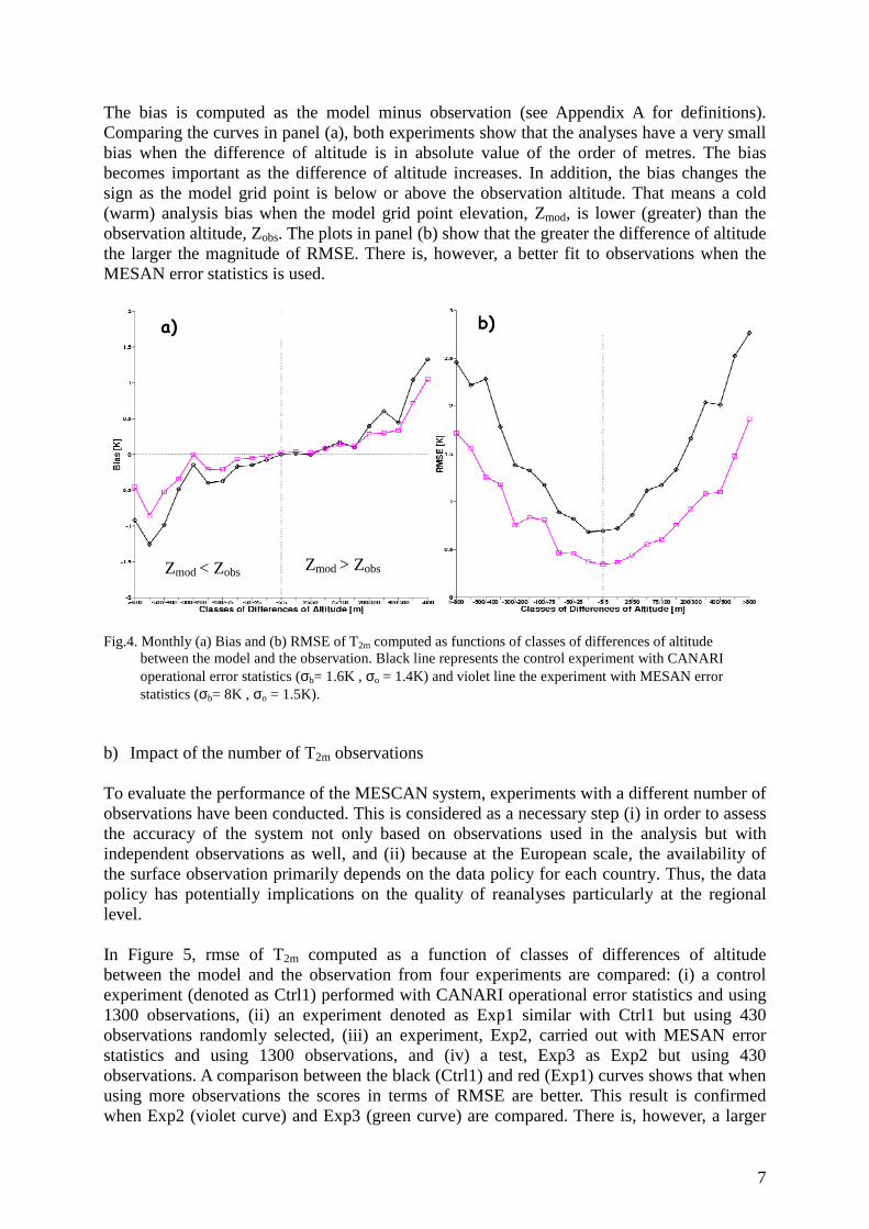
Fig. 3. Mean (a) bias and (b) rmse of T2m computed as functions of classes of differences of altitude between the model and the observation. The scores of ARPEGE model at 15km grid are represented by the blue line, background at 5.5km issued from downscaling ARPEGE field by the violet line, and black line stands for the analysis at 5.5km with CANARI operational error statistics (σb= 1.6K , σo = 1.4K). Scores computed for December 2009 – January 2010 using about 1300 observations. In order to assess the quality of the T2m fields, bias and rmse as functions of classes of differences of altitude between the model and the observation have been computed for two winter month: December 2009 and January 2010 using 6-hourly observations (used in the analyses). The results are plotted in Figure 3(a-b). Comparing the curves in panel (a), one may notice that ARPEGE model at 15km (blue line) is globally less biased than its downscaled fields at 5.5km (violet line), particularly over the complex orography (differences of altitude between the model, Zmod, and the observation, Zobs, greater that -300m). In addition, as shown in panel (b), the errors in terms of rmse are greater for ARPEGE downscaled fields at 5.5km than for those at lower resolution. The scores of the analysis system represented by the black line illustrate that the analysis successfully decreased the mean bias and the rmse. These results show that after downscaling, the quality of the fields obtained at high resolution may not always be improved although. In order to compare the results of various experiments, the following validation methods over France are considered: (a) impact of error statistics, (b) impact of the number of observations on the analysis, and (c) the evaluation of structure functions over orography. a) The impact of error statistics Figure 4 shows monthly bias (panel a) and the RMSE (panel b) of T2m computed as functions of classes of differences of altitude between the model and the observation for two experiments: the control (black line) which is performed with CANARI operational error statistics and structure function and an experiment with MESAN error statistics (violet line) and CANARI structure function. Note that CANARI structure function is isotropic and has the following form: exp(-r/L), where r is the distance between two points and L stands for the correlation length.

a) b)

Zmod < Zobs Zmod > Zobs Zmod > Zobs Zmod < Zobs

7

The bias is computed as the model minus observation (see Appendix A for definitions). Comparing the curves in panel (a), both experiments show that the analyses have a very small bias when the difference of altitude is in absolute value of the order of metres. The bias becomes important as the difference of altitude increases. In addition, the bias changes the sign as the model grid point is below or above the observation altitude. That means a cold (warm) analysis bias when the model grid point elevation, Zmod, is lower (greater) than the observation altitude, Zobs. The plots in panel (b) show that the greater the difference of altitude the larger the magnitude of RMSE. There is, however, a better fit to observations when the MESAN error statistics is used. Fig.4. Monthly (a) Bias and (b) RMSE of T2m computed as functions of classes of differences of altitude between the model and the observation. Black line represents the control experiment with CANARI operational error statistics (σb= 1.6K , σo = 1.4K) and violet line the experiment with MESAN error statistics (σb= 8K , σo = 1.5K).

b) Impact of the number of T2m observations To evaluate the performance of the MESCAN system, experiments with a different number of observations have been conducted. This is considered as a necessary step (i) in order to assess the accuracy of the system not only based on observations used in the analysis but with independent observations as well, and (ii) because at the European scale, the availability of the surface observation primarily depends on the data policy for each country. Thus, the data policy has potentially implications on the quality of reanalyses particularly at the regional level. In Figure 5, rmse of T2m computed as a function of classes of differences of altitude between the model and the observation from four experiments are compared: (i) a control experiment (denoted as Ctrl1) performed with CANARI operational error statistics and using 1300 observations, (ii) an experiment denoted as Exp1 similar with Ctrl1 but using 430 observations randomly selected, (iii) an experiment, Exp2, carried out with MESAN error statistics and using 1300 observations, and (iv) a test, Exp3 as Exp2 but using 430 observations. A comparison between the black (Ctrl1) and red (Exp1) curves shows that when using more observations the scores in terms of RMSE are better. This result is confirmed when Exp2 (violet curve) and Exp3 (green curve) are compared. There is, however, a larger

a) b)

Zmod < Zobs Zmod > Zobs

8

gap between curves from Exp2 and Exp3 than between Ctrl1 and Exp1 due to the fact that more weight is given to the observations in Exp2. When less observations are used, the difference of errors expressed in terms of RMSE between Exp1 and Exp3 is not as large as between Ctrl1 and Exp2. This is due to the fact that the lack of observations constrained the analysis to rely on the background. This result confirms the importance of the quality of the background fields in areas with sparse observations. Fig. 5. Monthly rmse of T2m computed as a function of classes of differences of altitude between the model and the observation for . The black line represents the control experiment (Ctrl1) performed with 1300 obs, the red line (Exp1) is for analyses performed with the same setting as the control but 430 obs, the violet line (Exp2) is for the test with MESAN σo and σb and 1300 obs, and the green line (Exp3) represents the test performed with MESAN σo and σb and 430 obs. c) Evaluation of structure functions over orography To evaluate the spatialization of the innovations, in particular over the complex orography, two experiments have been undertaken by using about 800 observations of T2m from stations at altitude lower than 300m: (i) a control experiment (hereafter denoted as e02_10) performed with CANARI operational settings, and (ii) an experiment (m01_14) with MESAN structure function and error statistics. Values of mean bias and RMSE computed for both experiments are indicated in Table 1. These scores have been computed by using the observations with the altitude below 300m used in the analyses, column (a), and then with about 500 independent observations above 300m, column (b).

Table 1. Monthly mean bias and rmse of T2m for December 2009 for analyses performed with observations below 300 m and verification against the observations (column a) used in the analyses (about 800 obs), and (column b) independent observations above 300m (about 500 obs). Units are K.

(a) (b) Experiments Bias RMSE Bias RMSE

Control experiment with CANARI σb , σo and structure function (e02_10)

-0.07 0.82 -0.132 1.860

Test analyses with MESAN σo ,σb and structure function (m01_14)

-0.01 0.73 -0.118 1.838

9

As indicated in Table 1 column (a), the analyses from the experiment m01_14 are almost unbiased and have a better fit to the observations. The scores in column (b) compared with those in column (a) illustrate that the quality of the analyses depends on the density of observations and the settings of error statistics. 4.2 Analysis of accumulated precipitation To ensure that the precipitation analysis schemes work properly, two experiments are performed: in physical space (hereafter denoted as MESCAN-RR) and in log-space (MESCAN-log) respectively. The analyses are generated for an extreme event that caused damages and casualties in its wake, and which occurred in the south east of France, mainly in Var county. The case study covers the period 06 UTC 15 June – 06 UTC 16 June 2010. The area of interest is encircled in Figure 6, which shows maps of 24-h accumulated precipitation valid at 0600 UTC 16 June 2010. All the maps are on a regular grid of 0.10. In panel (a), the map of the registered amounts of accumulated precipitation in 24 hours is plotted. Heavy precipitation amounts are particularly large: there is a peak value of 397 mm measured at Les Arcs and about 290 mm into an area of roughly 10km around this village (Vidauban: 289.7 mm, Le Luc: 286.2 mm). In summary, 2 stations reported precipitation amounts greater than 300mm, 10 reports indicated amounts greater than 200mm, and 23 rain gauges measured amounts greater than 100 mm.

Fig.6. Maps of 24-h accumulated precipitation projected on a regular grid of 0.10 valid at 0600 UTC 16 June 2010, for (a) observations, (b) ALADIN forecast field used as background, (c) analysis in physical space, and (d) analysis in log-space. In the experiments conducted, the precipitation analyses are generated with a background field at 5.5 km from the ALADIN-France model. The background is a 24-h forecast initiated at 0600 UTC, 15 June 2010 and covers the same period as observations. The ALADIN

a) Obs RR24MAX=397mm b) Aladin- fg: RR24MAX=77mm

c) MESCAN-RR: RR24MAX=265mm d) MESCAN-log: RR24MAX=277mm

10

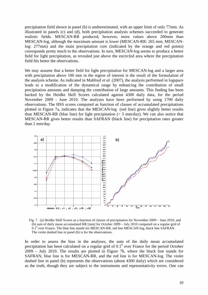
precipitation field shown in panel (b) is underestimated, with an upper limit of only 77mm. As illustrated in panels (c) and (d), both precipitation analysis schemes succeeded to generate realistic fields. MESCAN-RR produced, however, more values above 200mm than MESCAN-log, although the maximum amount is lower (MESCAN-RR: 265 mm; MESCAN-log: 277mm) and the main precipitation core (indicated by the orange and red points) corresponds pretty much to the observations. In turn, MESCAN-log seems to produce a better field for light precipitation, as revealed just above the encircled area where the precipitation field fits better the observations. We may assume that a better field for light precipitation for MESCAN-log and a larger area with precipitation above 100 mm in the region of interest is the result of the formulation of the analysis scheme. As indicated in Mahfouf et al. (2007), the analysis performed in logspace leads to a modification of the dynamical range by enhancing the contribution of small precipitation amounts and damping the contribution of large amounts. This finding has been backed by the Heidke Skill Scores calculated against 4300 daily data, for the period November 2009 - June 2010. The analyses have been performed by using 1700 daily observations. The HSS scores computed as function of classes of accumulated precipitations plotted in Figure 7a, indicates that the MESCAN-log (red line) gives slightly better results than MESCAN-RR (blue line) for light precipitation (< 5 mm/day). We can also notice that MESCAN-RR gives better results than SAFRAN (black line) for precipitation rates greater than 2 mm/day. Fig. 7. (a) Heidke Skill Scores as a function of classes of precipitation for November 2009 – June 2010, and (b) sum of daily mean accumulated RR [mm] for October 2009 – July 2010 computed on a regular grid of 0.10 over France. The blue line stands for MESCAN-RR, red line MESCAN-log, black line SAFRAN. The violet dashed line in panel (b) is for the observations. In order to assess the bias in the analyses, the sum of the daily mean accumulated precipitation has been calculated on a regular grid of 0.10 over France for the period October 2009 – July 2010. The results are plotted in Figure 7b, where the black line stands for SAFRAN, blue line is for MESCAN-RR, and the red line is for MESCAN-log. The violet dashed line in panel (b) represents the observations (about 4300 daily) which are considered as the truth, though they are subject to the instruments and representativity errors. One can

a) b)

11

note in panel (b) that in average, the analyses performed in log-space underestimate the precipitation amounts of around 50mm at the end of the period (after 270 days), whereas MESCAN-RR with the current settings generates precipitation fields which are closer to the observations. Since no tuning of error statistics and correlation length has been performed for any of the analysis schemes, these results should be regarded as relative. Further work is, however, necessary in this direction. In addition, several studies have shown that the change of variable necessary to satisfy the normal distribution assumption introduces a bias for analyses in log-space (Fortin, 2010; Lopez, 2011). The subsequent experiments have been performed in physical space due to the fact that the analyses in the log-space are more biased, which for hydrological purposes may have a negative impact. b) Impact of the number of observations To study the impact of the number of observations on the quality of precipitation analysis three tests are performed over France domain using MESCAN-RR with 1700 and 4300 observations respectively. The normalized difference of histograms and categorical scores such as HSS, equitable threat score, False Alarm Rate, Probability of Detection and Frequency Bias Index are computed as function of classes of 24-h accumulated precipitation for December 2009-January 2010 and June 2010. The following classes of precipitation rates are used: class A (0–0.2 mm/24h), class B (greater than 0.2–1 mm/24h), class C (1–2 mm/24h), class D (2.0–5.0 mm/24h), class E (5–10.0 mm/24h), class F (10–20 mm/24h), and class G (> 20 mm/24h).

Fig. 8. Heidke Skill Score (persistence) computed as function of classes of 24-h accumulated precipitation for (a) December 2009-January 2010, and (b) for June 2010. The black dotted line stands for the background,

blue solid (red dashed) line is for MESCAN-RR perform with 1700 obs and constant (variable) σo, red solid line is for MESCAN-RR with 4300 obs, and black solid line represents SAFRAN with 1700 obs..

When examining the plots in Figure 8(a-b), the poor quality of the background (black dotted line) in terms of HSS scores is revealed. The importance of a supplementary number of observations, particularly in winter period (panel a), is confirmed when comparing the scores computed (against 4300 observations) for the analyses performed using 1700 (blue line) and 4300 (red line) observations respectively. This finding points out the positive influence of the

a) Dec-Jan b) June

12

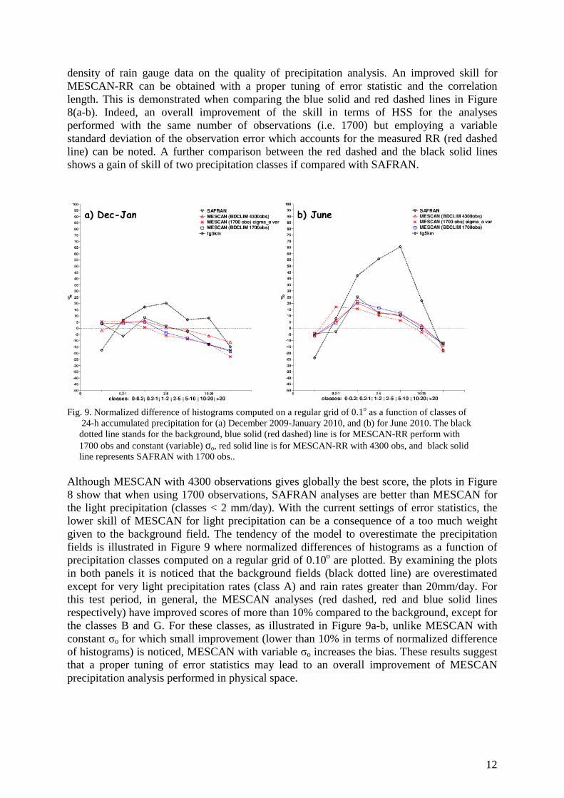
density of rain gauge data on the quality of precipitation analysis. An improved skill for MESCAN-RR can be obtained with a proper tuning of error statistic and the correlation length. This is demonstrated when comparing the blue solid and red dashed lines in Figure 8(a-b). Indeed, an overall improvement of the skill in terms of HSS for the analyses performed with the same number of observations (i.e. 1700) but employing a variable standard deviation of the observation error which accounts for the measured RR (red dashed line) can be noted. A further comparison between the red dashed and the black solid lines shows a gain of skill of two precipitation classes if compared with SAFRAN. Fig. 9. Normalized difference of histograms computed on a regular grid of 0.1o as a function of classes of 24-h accumulated precipitation for (a) December 2009-January 2010, and (b) for June 2010. The black dotted line stands for the background, blue solid (red dashed) line is for MESCAN-RR perform with 1700 obs and constant (variable) σo, red solid line is for MESCAN-RR with 4300 obs, and black solid line represents SAFRAN with 1700 obs.. Although MESCAN with 4300 observations gives globally the best score, the plots in Figure 8 show that when using 1700 observations, SAFRAN analyses are better than MESCAN for the light precipitation (classes < 2 mm/day). With the current settings of error statistics, the lower skill of MESCAN for light precipitation can be a consequence of a too much weight given to the background field. The tendency of the model to overestimate the precipitation fields is illustrated in Figure 9 where normalized differences of histograms as a function of precipitation classes computed on a regular grid of 0.10o are plotted. By examining the plots in both panels it is noticed that the background fields (black dotted line) are overestimated except for very light precipitation rates (class A) and rain rates greater than 20mm/day. For this test period, in general, the MESCAN analyses (red dashed, red and blue solid lines respectively) have improved scores of more than 10% compared to the background, except for the classes B and G. For these classes, as illustrated in Figure 9a-b, unlike MESCAN with constant σo for which small improvement (lower than 10% in terms of normalized difference of histograms) is noticed, MESCAN with variable σo increases the bias. These results suggest that a proper tuning of error statistics may lead to an overall improvement of MESCAN precipitation analysis performed in physical space.

a) Dec-Jan b) June

13

c) Indirect validation using a hydrological model In the case when the analysis does not initialize any numerical weather prediction model, a reliable approach to assess the accuracy of the analysis is to withhold a number of observations from the dataset which is to be further used for generating an analysis. Once the analysis is available it can be validated against the observations that have been kept apart. In our studies, the quality of precipitation analysis has been assessed not only by using independent observations but also ISBA-MODCOU coupled models. ISBA (Noilhan and Mahfouf, 1996; Boone et al., 1999) is a land surface model which derives energy budgets and surface water. The input data for the ISBA model are: temperature and humidity at 2m, wind speed at 10m, short- and long- wave incoming radiation, the amount and phase (rain/snow) of precipitation. The output surface runoff and soil water fluxes fields provided by ISBA are used as input data by the MODCOU hydrological model (Ledoux et al, 1989) to simulate the temporal evolution of the river flows at the spatial scale of a river watershed.

Fig.9. Daily river flow for the Seine river at Paris for different types of forcing.

To generate forcing for MODCOU, four experiments (performed by F. Besson) have been primarily conducted with ISBA by using different datasets: (i) precipitation, incoming radiation and 10-m wind velocity forecasted by the ALADIN model and MESCAN analyses for temperature and humidity at 2m (hereafter this experiment is referred to as CANARI experiment); (ii) radiation and wind from ALADIN and analyses of temperature, humidity and precipitation from MESCAN-RR (experiment called MESCAN); (iii) SAFRAN analyses (SAFRAN experiment); (iv) SAFRAN in the reanalysis mode (reanalysis experiment). The precipitation analyses have been carried out using 1700 observations except for SAFRAN in the reanalysis mode which has utilized about 4300 rain gauge observations. Here, it is worth mentioning that SAFRAN model is used in operational suite to provide input data for ISBA. ISBA output data have been used to force MODCOU to simulate the river flow on several watersheds. In Figure 9 the daily river flows for the Seine river at Paris observation location for the period October 2009 – June 2010 are plotted. The observations are represented by the dashed blue line. It can be noticed that the forcing provided by the forecasting model introduces a large overestimation of the river flow (red line). At the same time, MESCAN (green line) and both SAFRAN experiments (black and yellow lines) are close to the observations. Comparing the input data for CANARI and MESCAN experiments we can infer, not surprisingly, that the precipitation field is the main ingredient for estimating the river flow.

14

MESCAN-RR analysis scheme clearly improves the quality of the forcing in MESCAN experiment correcting the known overestimation of forecast precipitation field by ALADIN model.

Fig.10. Daily river discharge for the Rhone river at Beaucaire for different types of forcing. Analyzing the daily river discharges with different types of forcings for the Rhône river plotted in Figure 10, primarily we can notice that the difference between CANARI (red line) and the other experiments is not as large and obvious as for the Seine river (Figure 9). A comparison between MESCAN (green line) and SAFRAN (black line) show similar results except for the beginning of May and the entire month of June. The underestimation of the river flow by MESCAN compared with SAFRAN might be a result not solely of a lower snowpack accumulation throughout the Rhône watershed but also to the usage of the misleading information provided by the non-heated rain gauges in mountain areas during the winter season. d) Validation of snow depth at the observation location Another approach used for the indirect validation (work performed at CEN by M. Lafaysse) of precipitation analyses is to force the CROCUS model to simulate the snowpack. CROCUS is a unidimensional multi-layer snow model that simulates the evolution of snowpack characteristics as a function of weather conditions (Brun et al., 1989; 1992) developed at Météo-France, (CEN). As input data the model uses: temperature and humidity at 2m, wind speed at 10m, short- and long- waves incoming radiation and the amount and phase of precipitation. The evolution of the snowpack is derived by calculating variables such as temperature, liquid water content, density and snow type. CROCUS is used in the operational suite to assess the risk of avalanches. In the experiments conducted at CEN with CROCUS to simulate changes in the snow depth, the input data for the model is provided in turn by (i) SAFRAN; (ii) the ALADIN forecast model; (iii) MESCAN analysis system (temperature and humidity at 2m, and precipitation field) plus downward radiation and 10-m wind speed forecasted by ALADIN model. Primarily, the 6-hourly analyses for both T2m and RH2m are time interpolated to generate hourly values. Then, the data are projected at the observation location (at about 60 stations of various altitudes in the Alps) using two methods to obtain T2m values: (1) the nearest point to the validation location without any correction of altitude between the model and the

15

observation altitude (experiment denoted as MESCAN-v0); (2) a correction of altitude is performed by accounting for the mean temperature vertical gradient computed using the four nearest points (experiment called MESCAN-v1); and (3) as (2) but a spline function is used to hourly interpolate T2m (experiment MESCAN-v2). Fig. 11. Temporal evolution of snow depth at the observation location (a) Flaine, and (b) Bellecote nivose,

for different types of forcing: SAFRAN (red line), Aladin Forecast (grey line), MESCAN-v0 (blue) MESCAN-v1 (light blue), MESCAN-v2 (violet). Observations are represented by the black dots (Plots provided by M. Lafaysse).

The temporal interpolation of the analyzed RH2m has been done using the same methods as for the T2m while the approach of the nearest point to the observation location without any altitude correction has been chosen for the spatial fit. Regarding the 24-h precipitation analysis, the initial hourly values and precipitation phase have been derived base on the model precipitation. The final precipitation phase and implicitly the final hourly values have been computed as a function of hourly interpolated T2m at the observation location and altitude: rain (snow) if T2m is greater (lower) than 0.50C. For the separation rain/snow, the temperature threshold is used as in SAFRAN. The results for the winter period 2009-2010 show that in average SAFRAN analysis provides input data such as the CROCUS simulations are closer to the snow depth observations. At the same time MESCAN system improves the screen-level and precipitation fields from ALADIN model. Globally, the differences in terms of bias and rmse between MESCAN-v1 and MESCAN-v2 are very small. This finding shows that the method applied for time interpolation of T2m is not of major importance. On the contrary, the results are more sensitive with respect to the vertical correction of T2m due to the greater impact of the temperature gradient on the phase separation between liquid and solid precipitation. There are, however, results which show that the temporal evolution of snow depth simulated by CROCUS forced with MESCAN data can be close to the observations as well. This is revealed in Figure 11a when the observations (black dots) at Flaine station are compared with

a) FLAINE (1640m) b) Bellecote Nivose (3000m)

16

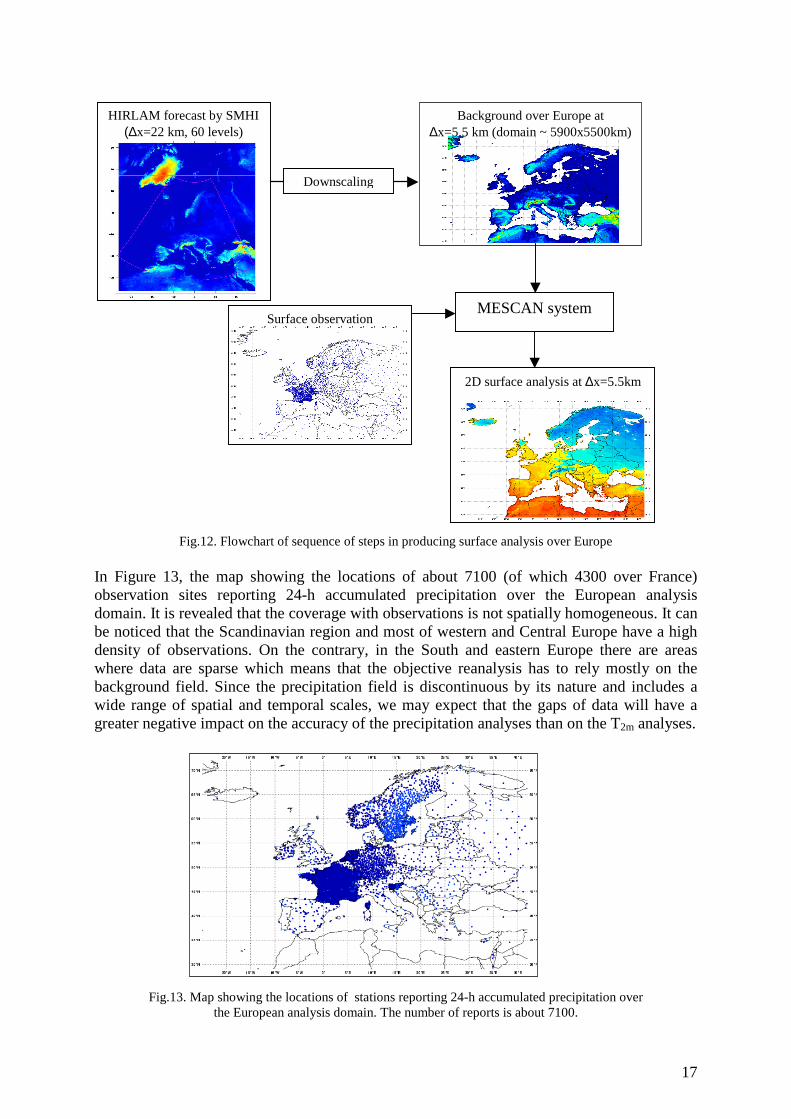
results from MESCAN-v0 (blue line), MESCAN-v1 (light blue), and MESCAN-v2 (violet) respectively. On the contrary, at Bellecote nivose (Figure 11b) the forcing provided by MESCAN analyses leads to results which are worse than when CROCUS simulations are performed with purely forecasted fields. Same opposite results are also found for SAFRAN (red line) when comparing with the observations: overestimation of snow depth revealed in panel (a), and a close fit to observations in panel (b). Overall, the scores of mean bias and rmse computed by M. Lafaysse at 57 stations reveal that the forcing provided by SAFRAN is better than that of MESCAN in the Alpine region: the bias is +6.7 cm (-8.6 cm) and the rmse is 27.8cm (36.6cm) for SAFRAN (MESCAN-v2). In order to improve the MESCAN analysis system, further experiments and validations at observation location are necessary. In addition one may consider for each observation location the usage of additional information as in SAFRAN: the usage of the past and present weather reports, the altitude of the isotherm of 0oC, fresh snow, rain gauge type (heated/non-heated), climatological values as a function of weather type, direction (north, south etc) and slope for each mountainous massif. Currently, MESCAN is not designed to use such type of specific information because it is very difficult to be gathered from the large number of National Meteorological Services across Europe. 4.3 Validation of MESCAN analyses over Europe In order to assess the quality of the analyses over Europe, validation experiments have been done for December 2009 and the year 2010. As such, the validation periods over European and French domains are overlapped. In addition, in order to comply with requirements set out in the deliverable D2.7 (verification of accumulated precipitation over the Alpine region) under responsibility of Meteo Swiss, precipitation analyses over Europe for the year 2008 have been generated as well. The flow diagram in Figure 12 presents the sequence of events in producing surface analysis over a domain of about 5900 by 5500 km covering Europe. The background used for screen-level variables is a 6-hour HIRLAM forecast downscaled from 22km at 5.5km. The HIRLAM forecasts are started at 0000, 0600, 1200 and 1800 UTC from a 3D-var reanalysis and are performed by SMHI. As for precipitation analysis, in order to span a 24-h period (06 UTC today – 06 UTC tomorrow), the background field is created as the sum of 12 hours accumulated precipitation: (fc00+18-fc00+06)+( fc12+18-fc12+06), where fc00+18 (fc00+06) is the 18-h (6-h) forecast started at 00 UTC, while fc12+18 (fc12+06) is the 18-h (6-h) forecast initiated at 12 UTC. The background created as the combination of forecasts of different ranges has been verified by SMHI to provide the best fields. A combination of forecasts of different ranges has been successfully tested in Mahfouf et al. (2007). To reduce the model spin-up problem the precipitation fields are selected not too close to the initial time (+6h), but not too far either (+18h) such as to have a good evolution of the large scale fields. The observations of T2m and RH2m are from French database mostly received through GTS, whereas the precipitation observations are from ECA&D database with additional rain gauge data from Météo-France and SMHI own networks. The merge of the precipitation observations from ECA&D (version 6), Météo-France and SMHI databases has been done at SMHI by T. Landelius.

17

Fig.12. Flowchart of sequence of steps in producing surface analysis over Europe In Figure 13, the map showing the locations of about 7100 (of which 4300 over France) observation sites reporting 24-h accumulated precipitation over the European analysis domain. It is revealed that the coverage with observations is not spatially homogeneous. It can be noticed that the Scandinavian region and most of western and Central Europe have a high density of observations. On the contrary, in the South and eastern Europe there are areas where data are sparse which means that the objective reanalysis has to rely mostly on the background field. Since the precipitation field is discontinuous by its nature and includes a wide range of spatial and temporal scales, we may expect that the gaps of data will have a greater negative impact on the accuracy of the precipitation analyses than on the T2m analyses.

Fig.13. Map showing the locations of stations reporting 24-h accumulated precipitation over the European analysis domain. The number of reports is about 7100.

HIRLAM forecast by SMHI (∆x=22 km, 60 levels)

2D surface analysis at ∆x=5.5km

Surface observation

Background over Europe at ∆x=5.5 km (domain ~ 5900x5500km)

MESCAN system

Downscaling

18

In fact, the number of available reports of T2m across the European domain is of about 3400, of which around 1300 are provided by the French network. a) Validation of the temperature at 2m In Figure 14, monthly bias and RMSE of T2m computed as a function of classes of differences of altitude between the model and the observation from three experiments performed at 5.5km grid-mesh are compared: (i) the control experiment, Ctrl1, performed over French domain with CANARI operational error statistics and structure function, (ii) Exp1 carried out over French domain as well, but with MESAN error statistics and CANARI structure function, and (iii) Exp2 as Exp1 but over Europe using 3700 observations (of which 1300 observations over France). We may recall that Ctrl1 and Exp1 are done using background fields from the ALADIN model and whereas Exp2 from the HIRLAM model. In the three experiments 1300 observations over France are utilized. Fig.14. Monthly (a) Bias and (b) RMSE of T2m (for December 2009) computed as functions of classes of differences of altitude between the model (Zmod) and the observation (Zobs). Black line represents the control (Ctrl1), red line (Exp1) is for the best fit to observations over France, and blue line (Exp2) the test performed over Europe domain with Hirlam background and evaluated over France. All the analyses are evaluated against the same observations. The comparison between the black (Ctrl1) and red (Exp1) lines shows better scores for Exp1 both in terms of bias and rmse. At the same time, when comparing the red (Exp1) and the blue (Exp2) lines we can notice that the scores are only slightly different, except over the complex orography (difference of altitude > 400 m) where Exp2 has a greater bias and larger errors in terms of rmse. As shown in panel (a), the bias is of the same sign for all experiments. The plots in panel (b) reveal that the greater the difference of altitude the larger the errors. These comparisons allow to consider that the T2m analyses over France performed with HIRLAM background are roughly of the same quality as those performed with the ALADIN background. In average for the year 2010, the T2m forecasted by the Hirlam model is overestimated. This is illustrated by the broad blue areas in Figure 15a which shows the map of annual mean AI of T2m. The analysis increments (AI) are calculated as the difference between the analysis and

a) b)

Zmod < Zobs Zmod < Zobs Zmod > Zobs Zmod > Zobs

19

the model background field. The AI are relevant in regions with sufficient observations. In areas with sparse data or without observations the AI are small because the difference between the analysis and the background is small. Negative values (blue colour) of AI signify an overestimation of the field by the model. A closer examination reveals that the model underestimates the T2m particularly over the Alpine region where the analysis increments have mean values of around 4oC . Fig. 15. Annual mean (a) analysis increments of T2m, and (b) analysis of T2m over Europe for the year 2010. Units are degrees Celsius. Figure 15b shows the map of the annual average T2m field produced by MESCAN analysis. We can notice the spatial variability of the T2m with decreasing values from South to North of Europe, and with negative values in the mountainous regions (the high Alps, Scandinavia and Iceland). b) Relative humidity at 2m The experiments conducted for the validation of the analysis of relative humidity at 2m over France (described in the report D2.10) and at the observation location (section 4.2, paragraph (c)) have not revealed any particular issue for this variable. These results allow us to focus more on the validation of the analysis of T2m and accumulated precipitation.

Fig.16. Annual average (a) analysis increments of RH2m, and (b) analysis of RH2m over Europe for the year 2010. Units are %.

a) b)

a) b)

20

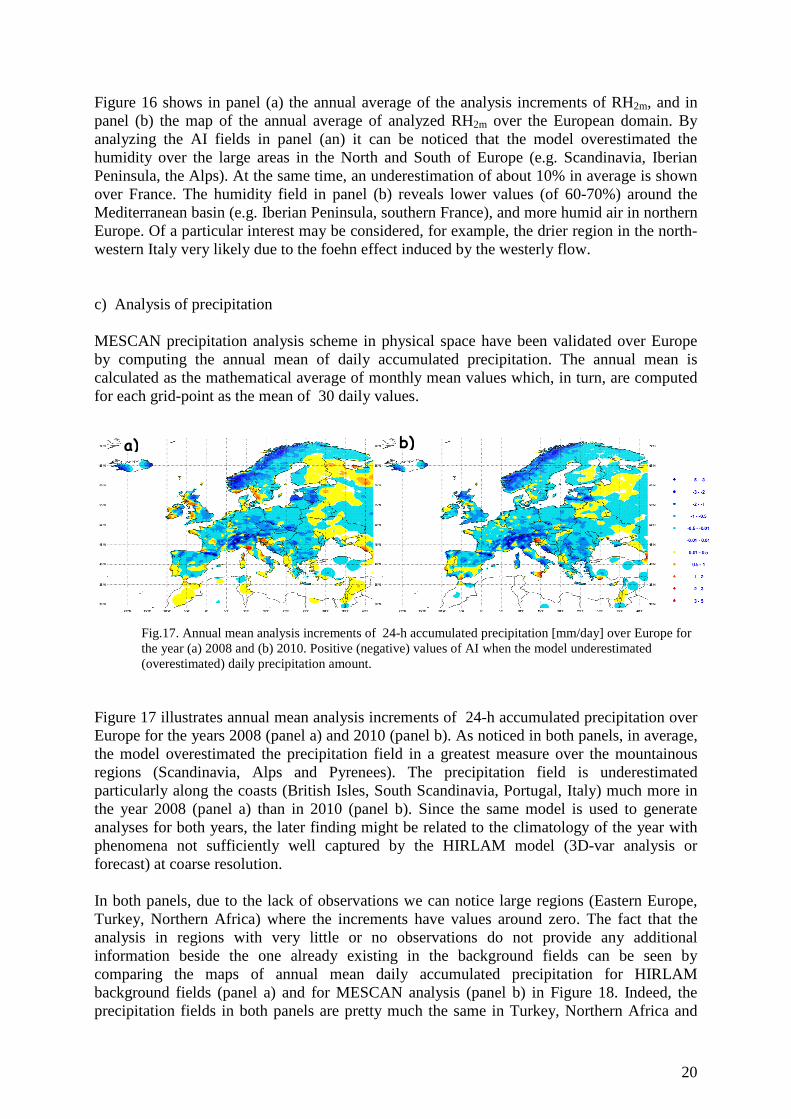
Figure 16 shows in panel (a) the annual average of the analysis increments of RH2m, and in panel (b) the map of the annual average of analyzed RH2m over the European domain. By analyzing the AI fields in panel (an) it can be noticed that the model overestimated the humidity over the large areas in the North and South of Europe (e.g. Scandinavia, Iberian Peninsula, the Alps). At the same time, an underestimation of about 10% in average is shown over France. The humidity field in panel (b) reveals lower values (of 60-70%) around the Mediterranean basin (e.g. Iberian Peninsula, southern France), and more humid air in northern Europe. Of a particular interest may be considered, for example, the drier region in the north-western Italy very likely due to the foehn effect induced by the westerly flow. c) Analysis of precipitation MESCAN precipitation analysis scheme in physical space have been validated over Europe by computing the annual mean of daily accumulated precipitation. The annual mean is calculated as the mathematical average of monthly mean values which, in turn, are computed for each grid-point as the mean of 30 daily values.

Fig.17. Annual mean analysis increments of 24-h accumulated precipitation [mm/day] over Europe for the year (a) 2008 and (b) 2010. Positive (negative) values of AI when the model underestimated (overestimated) daily precipitation amount.

Figure 17 illustrates annual mean analysis increments of 24-h accumulated precipitation over Europe for the years 2008 (panel a) and 2010 (panel b). As noticed in both panels, in average, the model overestimated the precipitation field in a greatest measure over the mountainous regions (Scandinavia, Alps and Pyrenees). The precipitation field is underestimated particularly along the coasts (British Isles, South Scandinavia, Portugal, Italy) much more in the year 2008 (panel a) than in 2010 (panel b). Since the same model is used to generate analyses for both years, the later finding might be related to the climatology of the year with phenomena not sufficiently well captured by the HIRLAM model (3D-var analysis or forecast) at coarse resolution. In both panels, due to the lack of observations we can notice large regions (Eastern Europe, Turkey, Northern Africa) where the increments have values around zero. The fact that the analysis in regions with very little or no observations do not provide any additional information beside the one already existing in the background fields can be seen by comparing the maps of annual mean daily accumulated precipitation for HIRLAM background fields (panel a) and for MESCAN analysis (panel b) in Figure 18. Indeed, the precipitation fields in both panels are pretty much the same in Turkey, Northern Africa and

a) b)

21

Russia. On the contrary, as illustrated in panel (b) compared with panel (a), the analysis “corrected” the precipitation field by reducing the amount of precipitation over large areas in Scandinavia, Central and Western Europe. However, if the background largely overestimates the precipitation field and no sufficiently dense observation network is available the analysis scheme cannot improve the precipitation field. By a closer examination of the maps, patterns of large amount of precipitation (greater than 3500 mm per year) along the western coast of Balkans can be identified. At the same time it can be noticed that the analysis has patterns of too dry areas in one of the Baltic countries (Latvia) while the model do not show any particular sign of dryness. This problem can be related to the systematic errors in the observations.

Fig.18. Total accumulated precipitation for over Europe for the year 2010, for (a) HIRLAM background fields, and (b) for MESCAN analysis. Units in mm.

Further work will be devoted to understand from where these potential errors come from in these areas, particularly for the year 2010. In this respect, the background precipitation fields and the observation dataset will be carefully investigated. 5. Ensemble based variational analysis A prototype ensemble-based two-dimensional variational (En2DVar) has been implemented within the project based on ideas in Liu et al. (2008 and 2009). The current OI systems for surface parameter analysis use parameterized covariance models that are fit to observation

Fig. 19. Example of covariance function (centred at the white point) arising from the rank deficient B matrix estimated with the NMC method using 124 members from December 2009 (left). Localization function for the same point (middle). Result after Shur product of localization and estimated B matrix (right).

b) a)

a) b) c)

22

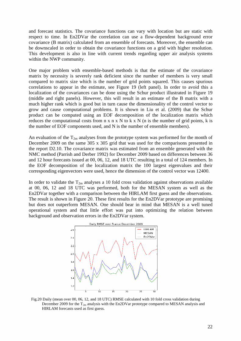
and forecast statistics. The covariance functions can vary with location but are static with respect to time. In En2DVar the correlation can use a flow-dependent background error covariance (B matrix) calculated from an ensemble of forecasts. Moreover, the ensemble can be downscaled in order to obtain the covariance functions on a grid with higher resolution. This development is also in line with current trends regarding upper air analysis systems within the NWP community. One major problem with ensemble-based methods is that the estimate of the covariance matrix by necessity is severely rank deficient since the number of members is very small compared to matrix size which is the number of grid points squared. This causes spurious correlations to appear in the estimate, see Figure 19 (left panel). In order to avoid this a localization of the covariances can be done using the Schur product illustrated in Figure 19 (middle and right panels). However, this will result in an estimate of the B matrix with a much higher rank which is good but in turn cause the dimensionality of the control vector to grow and cause computational problems. It is shown in Liu et al. (2009) that the Schur product can be computed using an EOF decomposition of the localization matrix which reduces the computational costs from n x n x N to k x N (n is the number of grid points, k is the number of EOF components used, and N is the number of ensemble members). An evaluation of the T2m analyses from the prototype system was performed for the month of December 2009 on the same 305 x 305 grid that was used for the comparisons presented in the report D2.10. The covariance matrix was estimated from an ensemble generated with the NMC method (Parrish and Derber 1992) for December 2009 based on differences between 36 and 12 hour forecasts issued at 00, 06, 12, and 18 UTC resulting in a total of 124 members. In the EOF decomposition of the localization matrix the 100 largest eigenvalues and their corresponding eigenvectors were used, hence the dimension of the control vector was 12400. In order to validate the T2m analyses a 10 fold cross validation against observations available at 00, 06, 12 and 18 UTC was performed, both for the MESAN system as well as the En2DVar together with a comparison between the HIRLAM first guess and the observations. The result is shown in Figure 20. These first results for the En2DVar prototype are promising but does not outperform MESAN. One should bear in mind that MESAN is a well tuned operational system and that little effort was put into optimizing the relation between background and observation errors in the En2DVar system.

Fig.20 Daily (mean over 00, 06, 12, and 18 UTC) RMSE calculated with 10 fold cross validation during December 2009 for the T2m analysis with the En2DVar prototype compared to MESAN analysis and HIRLAM forecasts used as first guess.

23

6. Summary and discussions The MESCAN analysis system has been objectively validated over France at 5.5 km grid spacing. The validation period spans a period of 9 month (October 2009 – June 2010) both for the screen-level variables and precipitation. The background is a short-range forecast from ALADIN-France model, downscaled at 5.5km grid-mesh. The observations used are from the high density French surface network. In order to assess the behaviour and the quality of MESCAN over the European domain, several experiments have been carried. For validation purposes, analyses of accumulated precipitation and temperature and humidity at 2m have been generated. The background is a short-range forecast from Hirlam model downscaled from 22 km to 5.5km. The observations are from Météo-France database for T2m and RH2m; daily precipitation observations are gathered by merging datasets from ECA&D, Météo-France and SMHI. The results obtained from the objective validation have shown that the MESCAN analysis system works properly (both over French and European domains) and for particular settings has better scores than CANARI and MESAN. There is still work to be done in order to improve the system, e.g adequate interpolation methods for downscaling fields, tuning of error statistics, a pre-processing of the precipitation observations particularly during the winter season and in the mountains. Regarding the precipitation analysis, studies for correcting the bias and employing an anisotropic structure function dependent on orography may be also addressed. Under the EURO4M framework devoted work (performed by M. Coustau) is on progress at Météo-France to use the MESCAN outputs to force the surface scheme SURFEX over Europe. Additional essential climate variable (snow depth, soil temperature and soil moisture, latent and sensible heat fluxes,) will be simulated and compared to observations. The MESCAN analysis system is implemented in cy38t1 of ARPEGE/IFS. The master logical key for activating the analysis of the screen-level variables is LMESCAN, whereas for precipitation analysis which uses a different structure function is LRRCAPA. Both keys have the default value set to false. Acknowledgments The studies in this report have been possible due to a close collaboration between teams in Météo-France (GMAP, BDCLIM, CEN) and SMHI. We very much appreciate support and fruitful discussions with GMAP colleagues, with special thanks to Françoise Taillefer and François Bouyssel for helpful suggestions. We are grateful to Ulf Andrae and Per Dahlgren (SMHI) for their enthusiastic support. Also, we much appreciate support and fruitful collaboration with the CEN team, particularly with M. Lafaysse and S. Morin during the evaluation of precipitation analysis at the observation location in the Alpine region. The research leading to these results has received funding from the European Union, Seventh Framework Programme (FP/2007-2013) under grant agreement no 242093.

24

Appendix A: Scores

In order to compare the accuracy of the analyses of T2m and RH2m, the following quantities are used:

a) the bias defined as bias= ∑ −N

=iii YX

1

)(N

1 (A1)

It measures a predominant or systematic anomaly in a given direction. A positive (negative) bias denotes an overestimation (underestimation) of the variable considered.

b) the root-mean-square error (rmse), defined as

rmse= ∑ −N

=iii YX

1

2)(N1

(A2)

where N is the total number of available observations, Xi denotes analyzed value at the closest grid point to the observation Yi. The rmse is influenced by one or more large, extreme, differences between model and observation values. To assess the quality of the analyses of 24-hour accumulated precipitation performed by MESCAN and SAFRAN, the computed quantities described hereafter are Heidke Skill Score and the normalized difference of histograms. The scores are computed with respect to the following classes of precipitation rates: class A (0–0.2 mm/24h), class B (greater than 0.2–1 mm/24h), class C (1–2 mm/24h), class D (2.0–5.0 mm/24h), class E (5–10.0 mm/24h), class F (10–20 mm/24h), and class G (> 20 mm/24h). c) The normalized difference of histograms (BF) is computed for each pre-defined class, as

the ratio of the difference between the number of forecasts of occurrence of class i, fiN , and

the number of observation of class i, oiN , to the total number of grid points, totN :

BF= 100N

N-Ntot

oi

fi ⋅ (A3)

BF=0 is for a perfect forecast. If BF is above (below) zero, it means overestimation (underestimation) of the selected variable.

d) Heidke Skill Score (HSS) is a measure of the skill of a two-class categorical forecasting schemes. A categorical forecast is an event which either occurs or does not occur. This type of forecast can be represented by a 2x2 contingency table, with elements defined as shown in Table A1.

Table A1: Schematic contingency table for categorical forecasts of a binary event. The number of observations are denoted by a, b, c and d. T is the total number.

Event observed Yes No

Yes a (hit) b (false alarm) a+b Event forecasted No c (miss) d (correct rejection) c+d a+c b+d T=a+b+c+d

In Table A1, four possible outcomes are possible:

1) hit: an event is forecasted and the event is observed;

25

2) false alarm: an event is forecasted but the event does not occur; 3) miss: an event is not forecasted but the event is observed; 4) correct rejection: an event is not forecasted and the event does not occur.

Heidke skill score is defined as,

HSS=R-T

R -da + (A4)

where T=a+b+c+d, and R=[(a+b)(a+c) + (b+d)(c+d)]/T. HSS is independent of T and ranges from -1 to 1. The HSS has a value of 1 for a perfect analysis or forecast, HSS = 0 means no skill, and if HSS <0, the forecast is worse than the reference forecast, R. Appendix B: List of Acronyms ARPEGE Action de Recherche Petite Echelle Grande Echelle CANARI Code d'Analyse Nécessaire a ARPEGE pour ses Rejets et son Initialisation CaPA Canadian Precipitation Analysis project CEN Centre d’Etude de Neige ECA&D European Climate Assessment & Dataset ECMWF European Centre for Medium-Range Weather Forecasts GTS Global Telecommunication System HIRLAM HIgh Resolution Limited Area Model IFS Integrated Forecasting System by ECMWF ISBA Interaction Sol-Biosphère-Atmosphère by Météo-France MESAN Mesoscale Analysis system by SMHI MESCAN A blend name between MESan and CANari. MODCOU MODélisation COUplée by Centre d’Informatique Géologique of the Ecole National

Supérior des Mines de Paris OI Optimal Interpolation SAFRAN Système d’Analyse Fournissant des Renseignements sur l’Atmosphère pour la Neige SMHI Swedish Meteorological and Hydrological Institute References Boone, A., J.C. Calvet, and J. Noilhan, 1999: Inclusion of a third soil layer in a land surface scheme using the force-restore method. J. Appl. Meteorol., 38, 1611-1630. Brun, E., E. Martin, V. Simon, C. Gendre, and C. Coléou, 1989: An energy and mass model of snow cover suitable for operational avalanche forecasting. J. Glaciol., 35 (121), 333-342. Brun, E., P. David, M. Sudul, and G. Brugnot, 1992: A numerical model to simulate snow cover stratigraphy for operational avalanche forecasting. J. Glaciol., 38 (128), 13-22. Daley, R. 1991: Atmospheric Data Analysis. Cambridge University Press: Cambridge, UK, 457 pp.

26

Durand, Y., E. Brun, L. Mérindol, G. Guyomarc’h, B. Lesaffre, and E. Martin, 1993: A meteorological estimation of relevant parameters for snow model. Ann. Glaciol., 18, 65-71. Fortin, V., Y. Kaheil, 2010: Real-time interpolation of precipitation observations: the limits of optimal interpolation, Atelier INSDC, 3-5 March 2010, Montréal, Canada. Häggmark, L., K.-I. Ivarsson, S. Gollvik, and P-O. Olofsson, 2000: Mesan, an operational mesoscale analysis system, Tellus, 52A, 2-20. Kalnay, E. 2003: Atmospheric Modeling, Data Assimilation and Predictability. Cambridge University Press: Cambridge, UK, 369 pp. Ledoux, E., G. Girard, G. de Marsily, and J. Deschenes, 1989: Spatially distributed modelling: Conceptual approach, coupling surface water and ground water, in Unsaturated flow hydrologic modelling - theory and practice, NATO ASI Series C, vol 275, edited by H. J. Morel-Seytoux, 435–454, Kluwer Academic, Norwell, Mass.. Liu, C., Q. Xiao, and B. Wang, 2009: An Ensemble-Based Four-Dimensional Variational Data Assimilation Scheme. Part II: Observing System Simulation Experiments with Advanced Research WRF (ARW). Mon. Wea. Rev., 137, 1687-1704. Lopez, P., 2011: Direct 4D-Var Assimilation of NCEP Stage IV Radar and Gauge Precipitation Data at ECMWF. Mon.Wea.Rev., 139, 2098-2116. Mahfouf, J.-F., B. Brasnett, and S. Gagnon, 2007: A Canadian precipitation analysis (CaPA) project: Description and preliminary results, Atmosphere-Ocean, 45:1, 1-17. Noilhan, J., and J.-F. Mahfouf, 1996: The ISBA land surface parameterization scheme, Global Planet. Change, 13, 145-159. Parrish, D., and J. Derber, 1992: The National Meteorological Center's spectral statistical interpolation analysis system. Mon. Wea. Rev., 120, 1747-1763. Saarinen, S. 2004: ODB User Guide (documentation available from ECMWF, Reading, UK). Taillefer, F., 2002: CANARI-Technical documentation (available from Météo-France, Toulouse, France).